ww.sciencedirect.com

b i o s y s t em s e n g i n e e r i n g 1 1 6 ( 2 0 1 3 ) 8 8e9 6

Available online at w

journal homepage: www.elsevier .com/locate/ issn/15375110

Research Paper

Foreground detection using loopy beliefpropagation

Gang J. Tu a,*, Henrik Karstoft b, Lene J. Pedersen a, Erik Jørgensen a

aDepartment of Animal Science, University of Aarhus, 8830 Tjele, DenmarkbDepartment of Engineering, University of Aarhus, 8000 Aarhus C, Denmark

a r t i c l e i n f o

Article history:

Received 22 December 2012

Received in revised form

27 April 2013

Accepted 20 June 2013

Published online 30 July 2013

* Corresponding author. Tel.: þ4587157849.E-mail address: gangjun.tu@agrsci.dk (G.J

1537-5110 ª 2013 The Authors. Published byhttp://dx.doi.org/10.1016/j.biosystemseng.201

This paper develops a simple and effective method for detection of sows and piglets in gray-

scale video recordings of farrowing pens. This approach consists of three stages: background

updating, calculation of pseudo-wavelet coefficients and foreground object segmentation. In

the first stage, the texture integration is used to update the background modelling (i.e. the

reference image). In the second stage, we apply an “a trous” wavelet transform on the current

reference image and then perform subtraction between the current original image and the

approximation of the current reference image. In the third stage, the pairwise relationships

betweenapixel and itsneighboursona factorgrapharemodelledbasedonthepseudo-wavelet

coefficients, and the image probabilities are approximated by using loopy belief propagation.

Experiments have shown promising results in extracting foreground objects from complex

farrowing pen scenes, such as sudden light changes and dynamic background as well as

motionless foreground objects.

ª 2013 The Authors. Published by Elsevier Ltd. on behalf of IAgre.

Open access under CC BY-NC-ND license.

1. Introduction sows and piglets often sleep for long periods; 3) Dynamic

The study of behaviour of livestock animals under farm con-

ditions with the assistance of automatic analysis of video re-

cordings is an open challenge in computer vision. In order to

detect simple behaviours of a sow (e.g. position, orientation,

movementetc.) ina farrowingpen,wefocusonsegmentationof

the sow, since the simple behaviours canbe efficiently detected

by using the shape of the sow in the segmented binary image if

the segmentation is correct. There are three major problems

with video segmentation in our farrowing pens: 1) Light

changes e the light sources in the farrowing house are often

turnedon/offduring theday;2)Motionless foregroundobjectse

. Tu).Elsevier Ltd. on behalf o3.06.011

backgrounde thenestingmaterials (e.g. straw) in the farrowing

pen are often moved around by sows and piglets.

A commonly used approach to extract foreground objects

from an image sequence is background subtraction, which is a

simple technique and has been widely used in real-time video

processing. Butmost existing background subtractionmethods

in recent surveys (Bouwmans, 2011; Brutzer, Hoferlin, &

Heidemann, 2011) are sensitive to sudden light changes and

motionless foreground objects. In the worst case, the whole

segmented image often appears as foreground inmost statisti-

calmodelswhenan illumination changeoccurs suddenly, anda

foreground object that becomes motionless cannot be

f IAgre. Open access under CC BY-NC-ND license.

Nomenclature

ABGt An approximation of BGt

BG0 An initial background model

BGt The background model at time t

bi The belief for a variable node i

ba The belief for a factor node a

E A set of edges

F A set of factor nodes

It A current image

ma / i The message from a factor node a to a variable

node i

N(i) A set of factor nodes, neighbours of a variable

node i

N(a) A set of variable nodes, neighbours of a factor

node a

P Joint probability distribution

p Marginal probability distribution

S(A,B) The similarity measure between two regions

A and B

SMt The texture similarity measure between the

current and reference images at time t

t Time

V A set of variable nodes

WBGt The wavelet coefficients of BGt

Wdiff The pseudo-wavelet coefficients

x ¼ fx1; :::; xi; :::; xng A vector of n random variables

xa A subset of x

f Local evidence

j Potential function

ni / a The message from a variable node i to a factor

node a

d Kronecker delta

b i o s y s t em s e ng i n e e r i n g 1 1 6 ( 2 0 1 3 ) 8 8e9 6 89

distinguished from a background object in a background

modelling and subtraction scheme such as a Gaussianmixture

model (GMM) (Stauffer & Grimson 2000).

In the past twenty years, a few algorithms for detecting and

tracking pigs have been introduced in the literature (Ahrendt,

Gregersen, & Karstoft, 2011; Hu & Xin, 2000; Lind, Vinther,

Hemmihgsen, & Hansen, 2005; Marchant & Schofield, 1993,

1995; Navarro-Jover et al., 2009; Perner, 2001; Shao & Xin, 2008;

Tillett, Onyango, &Marchant, 1997; Tillett 1991). The results for

most of these algorithms have not been discussed in relation to

complicated scenes (i.e. above main three problems). For

example, an advanced pig segmentation and tracking method

was developed by McFarlane and Schofield (1995) with special

emphasis on the initial segmentation and background estima-

tion. This method used a combination of image differencing

with respect to a median background and a Laplacian operator.

Themajor problemduring trackingwas the loss of tracking due

to large, unpredictable movements of the piglets, because the

tracking method required the objects to move (McFarlane &

Schofield, 1995). Shao and Xin (2008) developed a real-time

computer vision system that was used to segment the pigs,

detect the movements of the pigs and classify the thermal

behaviours of the pigs into cold, comfortable or warm/hot. The

prototype system was initially developed with paper-cut pigs

and then followed by tests with live pigs. In this system, image

segmentation was implemented using a global threshold that

converted grey level images to binary level, followed by

morphologicalfilteringandblob-fillingoperationstosmoothout

the images and remove themanure pieces (Shao&Xin, 2008). In

the motion detection stage, the images were modelled using a

shadingmodel (Skifstad& Jain, 1989). Themotiondetectionwas

based on a ratio of intensity levels of two consecutive images.

They assumed that the shading coefficient didn’t depend on

illumination and the illuminationcoefficients couldbe regarded

as uniform. If the intensity ratio was no longer constant, then

the motion appeared. Their approaches were not suitable for

video object segmentation in complex scenes, since they

assumed that the light didn’t change over time.

Factor graphs (Kschischang, Frey, & Loeliger, 2001) were

first studied in the context of error correction decoding and

have been used to formulate algorithms for a wide variety of

applications. Prior work has shown the relevance of factor

graphs to image processing (Drost & Singer, 2003). Belief

propagation (BP) (Yedidia, Freeman, &Weiss, 2003) is a widely

used technique for approximate inference in graphical

models. It uses the idea of passing local messages around the

nodes through edges and works for arbitrary potential func-

tions. Loopy BP (Yedidia et al., 2000) is an extension of the BP

framework developed by Pearl (1988), and often yields very

good approximations in stereo vision (Felzenszwalb &

Huttenlocher, 2006), motion tracking (Yin & Collins, 2007) etc.

Theundecimatedwavelet transform(WT) (Starck,Murtagh,&

Bijaoui,1998)doesnot incorporate thedownsamplingoperations

and upsamples the coefficients of the lowpass and highpass

filters at each level. Thus, the approximation and detail co-

efficients at each level are the same length as the original signal.

The number ofwavelet coefficients does not shrink between the

transform levels. This additional information can be very useful

for better analysis and understanding of signal properties.

In this paper, we present a simple and effective method to

segment sows and piglets in the complex scene of farrowing

pens. Our method has three stages: 1) Background updating:

the texture integration is used to update the reference image;

2) Calculation of pseudo-wavelet coefficients: an “a trous”

wavelet transform is applied to the current reference image

and then the subtraction operation is performed between the

current original image and the approximation of the current

reference image; 3) Foreground object segmentation: the

pairwise relationships between a pixel and its neighbours on a

factor graph are modelled based on the pseudo-wavelet co-

efficients, and the image probabilities are approximated by

using loopy belief propagation. The experimental results show

that our method can substantially reduce the above three

problems in our application.

2. The methods

2.1. Belief propagation on factor graph

Let x ¼ fx1;.; xi;.; xng be a vector of n random variables,

where i˛V ¼ f1; 2; :::; ng. We consider a joint distribution

b i o s y s t em s e n g i n e e r i n g 1 1 6 ( 2 0 1 3 ) 8 8e9 690

P(x1,...,xi,...,xn) and assume that it factors into a product of non-

negative functions:

Pðx1; :::; xi; :::; xnÞ ¼ 1Z

Yni¼1

fiðxiÞYma¼1

jaðxaÞ (1)

wherefiðxiÞ represents“localevidence”orpriordataonthestates

ofxi,ja(xa)hasargumentxa that isasubsetofx ¼ fx1; :::; xi; :::; xng,and Z is a normalisation constant. In the context of graphical

models such a bipartite graph representation is referred to as a

factor graph (Kschischang et al., 2001), which is a tuple (V,F,E )

consisting of a setV of variable nodes, a set F of factor nodes, and

a set E4ðV � FÞ edges having one endpoint at a variable node

and the other at a factor node. LetNðiÞ ¼ fa˛F: ði;aÞ˛Eg stand for

all factor nodes in which are neighbours of variable node i and

NðaÞ ¼ fi˛V: ði;aÞ˛Eg stand for all variable nodes which are

neighbours of factor node a. In actuality, we ignore the constant

Z in the factor graph model because the value of Z is not

easily determined and will not have an effect on the final result

(Drost & Singer, 2003).We can define fiðxiÞ ¼ 1 (i.e. uniform local

evidence) for every xi in a factor graph.

Loopy BP works by exchanging messages between nodes.

Each node sends and receives messages until a stable situa-

tion is reached. There are two kinds of messages (Yedidia,

Freeman, & Weiss, 2005): messages ni / a(xi) sent from a var-

iable node i to a factor node a, and messages ma / i(xi)sent

from a factor node a to a variable node i. With our definition of

the joint probability measure (see Eq. (1)), the messages are

updated according to the following rules:

ma/iðxiÞ)Xxa=xi

jaðxaÞY

j˛NðaÞ=ihj/a

�xj

�(2)

hi/aðxiÞ)fiðxiÞY

b˛NðiÞ=amb/iðxiÞ (3)

Themessages ni / a(xi) are usually initialised to the uniform

vector. When the algorithm converges (i.e. messages do not

change), one calculates the approximate marginal p(xi) or

p(xa), also known as belief bi(xi) or ba(xa):

Fig. 1 e Factor graph corresponding to a 3 3 3 grid, variable no

edges are drawn as undirected edges between variable and facto

Right: Passing factor-to-variable messages by Eq. (3).

pðxiÞzbiðxiÞffiðxiÞa˛NðiÞ

ma/iðxiÞ (4)

Y

pðxaÞzbaðxaÞfijaðxaÞY

i˛NðaÞhi/aðxiÞ (5)

In this paper, we simply use an 8-connected spatial neigh-

bourhood system, which is also called a second-order neigh-

bourhood system. Figure 1 shows the nine pixels and

corresponding factor graph in an image. We set fiðxiÞ ¼ 1. The

pairwise potential function jij(xi, xj) corresponds to the

matching cost computation between xi and xj. The potential

function takes the form of a pairwise Potts model:

jijðxi; xjÞ ¼ expðJdxixj Þ, where J is a parameter which determines

how much the neighbouring locations i and j influence each

other regarding their values of xi and xj, d and exp are the

Kronecker delta and exponential functions, respectively. We

chose J ¼ 2 in our experiment.

2.2. Wavelet representation of image

We perform an “a trous” WT (Mallat, 1999; Starck et al., 1998)

using a cubic spline on each reference image. The WT is

undecimated and produces two images at each scale, one is

the approximation A2j and the other one is the wavelet co-

efficients W2j , where j˛Z.

2.3. Background updating

At the start, we assume that the sequence begins with the

background in the absence of foreground. The initial back-

ground model BG0 is constructed as:

BG0ðpÞ ¼PN

i¼0IiðpÞN

(6)

where Ii( p) is the intensity of pixel p of the ith image, and N is

the number of images used to construct the background

model (i.e. the reference image).

des are drawn as B, factor nodes are drawn as , and the

r nodes. Left: Passing variable-to-factor messages by Eq. (2).

Table 1 e The pseudo-code of the proposed algorithm.

b i o s y s t em s e ng i n e e r i n g 1 1 6 ( 2 0 1 3 ) 8 8e9 6 91

After obtaining the initial reference image, the reference

image must be updated at every time t in order to accommo-

date for background dynamics such as illumination changes. In

general, a statistical background model (e.g. GMM (Stauffer &

Grimson 2000)) generates large areas of false foreground

when there are quick lighting changes. In order to make our

method more robust to sudden illumination changes, the

texture information is used to update the reference image. The

gradient value is less sensitive to lighting changes and is able to

derive an accurate local texture differencemeasure (Li & Huang

2002). Here, a texture similarity measure SM between the cur-

rent image and the reference image at time t is defined as

SMtðpÞ ¼P

u˛NðpÞ2$��gc

tðuÞ��$��gr

tðuÞ��$cosqP

u˛NðpÞ�kgc

tðuÞk2 þ kgrtðuÞk2

� (7)

where N( p) denotes the 3 � 3 neighbourhood centred at pixel

p, gct and gr

t are gradient vectors of the current image and the

reference image at time t, respectively, and q is the angle

between the two vectors. The gradient vectors are obtained

by the Sobel operator. If the texture does not change between

the current image and the reference image at pixel p, then

Fig. 2 e The flowchart of our algorithm. The backgroundmodel is

SM( p) z 1 (Li & Huang 2002). The current reference image at

time t is updated as

BGtðpÞ ¼�ItðpÞ; if SMtðpÞ > ssm;BG0ðpÞ; otherwise;

(8)

where SMtðpÞ > ssm corresponds to the texture not changing

between the two images at pixel p (i.e. the value of pixel p in

BGt is the value of pixel p in It, because the pixel p in It is a

background pixel). Obviously, there are some foreground

pixels of the current image It that satisfy SMtðpÞ > ssm when the

strong illumination change occurs at time t. Thus, those pixels

become the false background pixels of BGt.

In order to reduce the false background pixels in the cur-

rent reference image BGt, we apply the threshold technique.

Let Ct ¼ fx: SMtðxÞ > ssm^x˛BGtg be a set of pixels. The false

background pixel p in BGt can be removed by

BGCtt ðpÞ ¼

�BG0ðpÞ; if BGtðpÞ > slight^p˛Ct;BGtðpÞ; otherwise;

(9)

where slight is a threshold which is easily found, because the

pixel value should be relatively high if it belongs to Ct.

defined by Eq. (6). Loop BP stands for loop belief propagation.

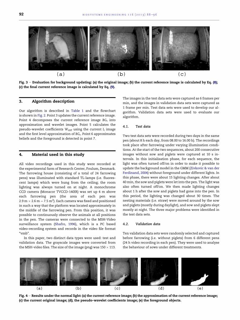
Fig. 3 e Evaluation for background updating: (a) the original image; (b) the current reference image is calculated by Eq. (8);

(c) the final current reference image is calculated by Eq. (9).

b i o s y s t em s e n g i n e e r i n g 1 1 6 ( 2 0 1 3 ) 8 8e9 692

3. Algorithm description

Our algorithm is described in Table 1 and the flowchart

is shown in Fig. 2. Point 3 updates the current reference image.

Point 4 decomposes the current reference image BGt into

approximation and wavelet images. Point 5 calculates the

pseudo-wavelet coefficients Wdiff using the current It image

and the first level approximation of BGt. Point 6 approximates

beliefs and the foreground is detected in point 7.

4. Material used in this study

All video recordings used in this study were recorded at

the experimental farm of Research Center, Foulum, Denmark.

The farrowing house (consisting of a total of 24 farrowing

pens) was illuminated with standard TL-lamps (i.e. fluores-

cent lamps) which were hung from the ceiling; the room

lighting was always turned on at night. A monochrome

CCD camera (Monacor TVCCD-140IR) was set up 4 m above

each farrowing pen (the area of each pen was

2.9m� 2.6 m¼ 7.5 m2). Each camera was fixed and positioned

in such a way that the platform was located approximately in

the middle of the farrowing pen. From this position, it was

possible to continuously observe the animals at all positions

in the pen. The cameras were connected to the MSH-Video

surveillance system (Shafro, 1996), which is a PC based

video-recording system and records in the video file format

“vmb”.

In this paper, two distinct data types were used: test and

validation data. The grayscale images were converted from

theMSH-video files. The size of the image (png) was 150� 113.

Fig. 4 e Results under the normal light: (a) the current reference i

(c) the current original image; (d); the pseudo-wavelet coefficien

The images in the test data sets were captured as 6 frames per

min, and the images in validation data sets were captured as

1 frame per min. Test data sets were used to develop our al-

gorithm. Validation data sets were used to evaluate our

algorithm.

4.1. Test data

Two test data sets were recorded during two days in the same

pen (about 8 h each day, from 08.00 to 16.00 h). The recordings

took place after farrowing under varying illumination condi-

tions. At the start of the two sequences, about 200 consecutive

images without sow and piglets were captured at 10 s in-

tervals. In this initialisation phase, for each sequence, the

light was often turned off/on in order to make it possible to

update the backgroundmodel in the GMM (Zivkovic & van der

Ferdinand, 2004) without foreground under different lights. In

this phase, there were about 15 lighting changes. After about

40min, the sow and pigletswere let into the pen. The lightwas

also often turned off/on. We then made lighting changes

about 1 h after the sow and piglets had gone into the pen. In

this period, the lighting was changed about 30 times. The

nesting materials (i.e. straw) were moved around by the sow

and piglets (mostly during daylight), and sow and piglets slept

mostly at night. The three major problems were identified in

the test data sets.

4.2. Validation data

Ten validation data sets were randomly selected and captured

before farrowing (i.e. without piglets) from 6 different pens

(24 h video recording in each pen). They were used to analyse

the behaviour of sows under different treatments.

mage; (b) the approximation of the current reference image;

ts image; (e) the foreground objects.

Fig. 5 e Results under the sudden light change: (a) the current reference image; (b) the approximation of the current reference

image; (c) the current original image; (d) the pseudo-wavelet coefficients image; (e) the foreground objects.

b i o s y s t em s e ng i n e e r i n g 1 1 6 ( 2 0 1 3 ) 8 8e9 6 93

5. Evaluation criteria

In order to test the effectiveness of our methods, we set the

following criteria to evaluate the original images and the

segmented results.

� We manually evaluated the area of the sow in all images

in the validation data. The evaluated area was used for

comparison with the corresponding shape of the sow in the

segmented binary image.

� All segmented images in the validation data were visually

evaluated, and classified into three scale groups:

1. Full Segmentation (FS): The shape of the sow was

segmented over 90% of the manually evaluated area.

2. Partial Segmentation (PS): The shape of the sow was

segmented between 80% and 90% of the manually

evaluated area.

3. Cannot Segment (CNS): a) There were two or more

separated regions; b) Thereweremany false foreground

areas in the segmented image; c) The shape of the sow

was segmented in less than 80% of the manually eval-

uated area.

6. Experimental results

The algorithm was implemented using Matlab and Cþþ.

The parameter N in Eq. (6) was set at 10 (10 images used

to construct background model) and all the background

images were selected under different light conditions. Based

on our data analysis, the thresholds ssm in Eq. (8) and slight in

Eq. (9) were set at 0.8 and 184, respectively. Our algorithm runs

at a speed of 4 frames s�1, and this speed is satisfactory for our

Fig. 6 e Comparison of the GMM-based method with our metho

(b) the result of the GMM-based method; (c) the result of our pro

application. In order to compare other existing methods, the

GMM-based method (Zivkovic & van der Ferdinand, 2004) was

used and applied to every set of test data. The first 200 images

(without foreground) of every set were the recent history data

for the GMM-based method.

In this section,we qualitatively and quantitatively evaluate

the segmented images. It is very important to note that no

post-processing technique, such as morphological operator,

was used in our algorithm.

6.1. Evaluation for background model

The aim of background updatingwas to get the value of pixel p

in the current reference image BGt which should be as close to

the value of pixel p in the current image It as possible, if the

texture did not change between the two images at pixel p.

Because we used the subtraction operation (see point 5 in

Table 1) after the reference image was updated.

Figure 3 gives an example for the background updating in

the test data. We firstly applied Eq. (8) on two images: the

current image It (Fig. 3a) and the image BG0 (see Eq. (6)), to get

the current reference image that is shown in Fig. 3b. As one

can see, some foreground pixels still persist in Fig. 3b. Using

Eq. (9), the final current reference image (Fig. 3c) is obtained by

a combination of Fig. 3b and the image BG0.

6.2. Qualitative analysis

In order to performqualitative evaluation of our segmentation

algorithm, we have selected the following 3 segmented im-

ages from the test data sets, which represent the general re-

sults under normal light (i.e. the light off in the farrowing pen),

sudden light change (the light was turned on in the farrowing

pen) and sudden strong illumination change (the extra light

d under sudden strong illumination: (a) the original image;

posed method.

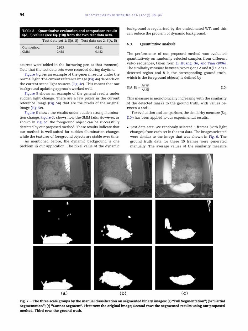
Table 2 e Quantitative evaluation and comparison result:S(A, B) values (see Eq. (10)) from the two test data sets.

Test data set 1: S(A, B) Test data set 2: S(A, B)

Our method 0.923 0.911

GMM 0.438 0.482

b i o s y s t em s e n g i n e e r i n g 1 1 6 ( 2 0 1 3 ) 8 8e9 694

sources were added in the farrowing pen at that moment).

Note that the test data sets were recorded during daytime.

Figure 4 gives an example of the general results under the

normal light. The current reference image (Fig. 4a) depends on

the current scene light sources (Fig. 4c). This means that our

background updating approach worked well.

Figure 5 shows an example of the general results under

sudden light change. There are a few pixels in the current

reference image (Fig. 5a) that are the pixels of the original

image (Fig. 5c).

Figure 6 shows the results under sudden strong illumina-

tion change. Figure 6b shows how the GMM fails. However, as

shown in Fig. 6c, the foreground object can be successfully

detected by our proposed method. These results indicate that

our method is well-suited for sudden illumination changes

while the textures of foreground objects are stable over time.

As mentioned before, the dynamic background is one

problem in our application. The pixel value of the dynamic

Fig. 7 e The three scale groups by the manual classification on se

Segmentation”; (c) “Cannot Segment”. First row: the original im

method. Third row: the ground truth.

background is regularised by the undecimated WT, and this

can reduce the problem of dynamic background.

6.3. Quantitative analysis

The performance of our proposed method was evaluated

quantitatively on randomly selected samples from different

video sequences, taken from Li, Huang, Gu, and Tian (2004).

The similaritymeasure between two regionsA and B (i.e.A is a

detected region and B is the corresponding ground truth,

which is the foreground objects) is defined by

SðA;BÞ ¼ AXBAWB

(10)

This measure is monotonically increasing with the similarity

of the detected masks to the ground truth, with values be-

tween 0 and 1.

For evaluation and comparison, the similaritymeasure (Eq.

(10)) has been applied to our experimental results.

� Test data sets: We randomly selected 5 frames (with light

changes) from each set in the test data. The images selected

were similar to the image that was shown in Fig. 6. The

ground truth data for these 10 frames were generated

manually. The average values of the similarity measure

gmented binary images: (a) “Full Segmentation”; (b) “Partial

age; Second row: the segmented results using our proposed

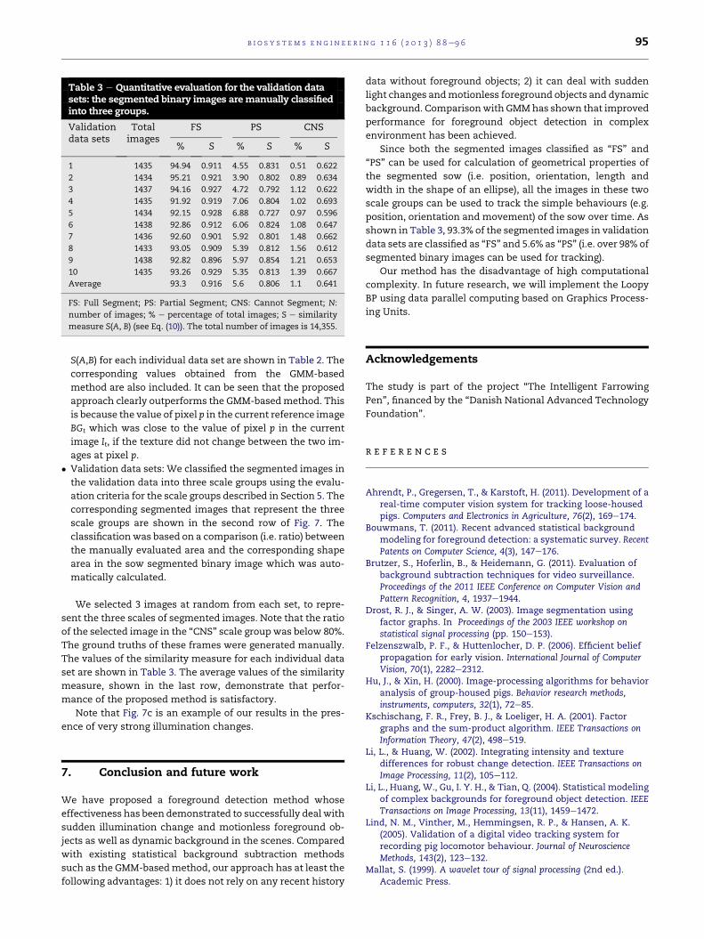
Table 3 e Quantitative evaluation for the validation datasets: the segmented binary images aremanually classifiedinto three groups.

Validationdata sets

Totalimages

FS PS CNS

% S % S % S

1 1435 94.94 0.911 4.55 0.831 0.51 0.622

2 1434 95.21 0.921 3.90 0.802 0.89 0.634

3 1437 94.16 0.927 4.72 0.792 1.12 0.622

4 1435 91.92 0.919 7.06 0.804 1.02 0.693

5 1434 92.15 0.928 6.88 0.727 0.97 0.596

6 1438 92.86 0.912 6.06 0.824 1.08 0.647

7 1436 92.60 0.901 5.92 0.801 1.48 0.662

8 1433 93.05 0.909 5.39 0.812 1.56 0.612

9 1438 92.82 0.896 5.97 0.854 1.21 0.653

10 1435 93.26 0.929 5.35 0.813 1.39 0.667

Average 93.3 0.916 5.6 0.806 1.1 0.641

FS: Full Segment; PS: Partial Segment; CNS: Cannot Segment; N:

number of images; % e percentage of total images; S e similarity

measure S(A, B) (see Eq. (10)). The total number of images is 14,355.

b i o s y s t em s e ng i n e e r i n g 1 1 6 ( 2 0 1 3 ) 8 8e9 6 95

S(A,B) for each individual data set are shown in Table 2. The

corresponding values obtained from the GMM-based

method are also included. It can be seen that the proposed

approach clearly outperforms the GMM-basedmethod. This

is because the value of pixel p in the current reference image

BGt which was close to the value of pixel p in the current

image It, if the texture did not change between the two im-

ages at pixel p.

� Validation data sets: We classified the segmented images in

the validation data into three scale groups using the evalu-

ation criteria for the scale groups described in Section 5. The

corresponding segmented images that represent the three

scale groups are shown in the second row of Fig. 7. The

classificationwas based on a comparison (i.e. ratio) between

the manually evaluated area and the corresponding shape

area in the sow segmented binary image which was auto-

matically calculated.

We selected 3 images at random from each set, to repre-

sent the three scales of segmented images. Note that the ratio

of the selected image in the “CNS” scale group was below 80%.

The ground truths of these frames were generated manually.

The values of the similarity measure for each individual data

set are shown in Table 3. The average values of the similarity

measure, shown in the last row, demonstrate that perfor-

mance of the proposed method is satisfactory.

Note that Fig. 7c is an example of our results in the pres-

ence of very strong illumination changes.

7. Conclusion and future work

We have proposed a foreground detection method whose

effectiveness has been demonstrated to successfully deal with

sudden illumination change and motionless foreground ob-

jects as well as dynamic background in the scenes. Compared

with existing statistical background subtraction methods

such as the GMM-basedmethod, our approach has at least the

following advantages: 1) it does not rely on any recent history

data without foreground objects; 2) it can deal with sudden

light changes andmotionless foreground objects and dynamic

background. Comparisonwith GMMhas shown that improved

performance for foreground object detection in complex

environment has been achieved.

Since both the segmented images classified as “FS” and

“PS” can be used for calculation of geometrical properties of

the segmented sow (i.e. position, orientation, length and

width in the shape of an ellipse), all the images in these two

scale groups can be used to track the simple behaviours (e.g.

position, orientation and movement) of the sow over time. As

shown in Table 3, 93.3% of the segmented images in validation

data sets are classified as “FS” and 5.6% as “PS” (i.e. over 98% of

segmented binary images can be used for tracking).

Our method has the disadvantage of high computational

complexity. In future research, we will implement the Loopy

BP using data parallel computing based on Graphics Process-

ing Units.

Acknowledgements

The study is part of the project “The Intelligent Farrowing

Pen”, financed by the “Danish National Advanced Technology

Foundation”.

r e f e r e n c e s

Ahrendt, P., Gregersen, T., & Karstoft, H. (2011). Development of areal-time computer vision system for tracking loose-housedpigs. Computers and Electronics in Agriculture, 76(2), 169e174.

Bouwmans, T. (2011). Recent advanced statistical backgroundmodeling for foreground detection: a systematic survey. RecentPatents on Computer Science, 4(3), 147e176.

Brutzer, S., Hoferlin, B., & Heidemann, G. (2011). Evaluation ofbackground subtraction techniques for video surveillance.Proceedings of the 2011 IEEE Conference on Computer Vision andPattern Recognition, 4, 1937e1944.

Drost, R. J., & Singer, A. W. (2003). Image segmentation usingfactor graphs. In Proceedings of the 2003 IEEE workshop onstatistical signal processing (pp. 150e153).

Felzenszwalb, P. F., & Huttenlocher, D. P. (2006). Efficient beliefpropagation for early vision. International Journal of ComputerVision, 70(1), 2282e2312.

Hu, J., & Xin, H. (2000). Image-processing algorithms for behavioranalysis of group-housed pigs. Behavior research methods,instruments, computers, 32(1), 72e85.

Kschischang, F. R., Frey, B. J., & Loeliger, H. A. (2001). Factorgraphs and the sum-product algorithm. IEEE Transactions onInformation Theory, 47(2), 498e519.

Li, L., & Huang, W. (2002). Integrating intensity and texturedifferences for robust change detection. IEEE Transactions onImage Processing, 11(2), 105e112.

Li, L., Huang, W., Gu, I. Y. H., & Tian, Q. (2004). Statistical modelingof complex backgrounds for foreground object detection. IEEETransactions on Image Processing, 13(11), 1459e1472.

Lind, N. M., Vinther, M., Hemmingsen, R. P., & Hansen, A. K.(2005). Validation of a digital video tracking system forrecording pig locomotor behaviour. Journal of NeuroscienceMethods, 143(2), 123e132.

Mallat, S. (1999). A wavelet tour of signal processing (2nd ed.).Academic Press.

b i o s y s t em s e n g i n e e r i n g 1 1 6 ( 2 0 1 3 ) 8 8e9 696

Marchant, J. A., & Schofield, C. P. (1993). Extending the snakeimage processing algorithm for outlining pigs in scenes.Computers and Electronics in Agriculture, 8(4), 261e275.

McFarlane, N. J. B., & Schofield, C. P. (1995). Segmentation andtracking of piglets in images. Machine Vision and Applications,8(3), 187e193.

Navarro-Jover, J. M., Alcaniz-Raya, M., Gomez, V., Balasch, S.,Moreno, J.R.,Grau-Colomer,V., etal. (2009).Anautomaticcolour-based computer vision algorithm for tracking the position ofpiglets. Spanish Journal of Agricultural Research, 7(3), 535e549.

Pearl, J. (1988). Probabilistic reasoning in intelligent systems. SanFrancisco, CA, USA: Morgan Kaufmann Publishers Inc.

Perner, P. (2001). Motion tracking of animals for behavior analysis.In Proceeding IWVF-4 proceedings of the 4th internationalworkshop on visual form (pp. 779e786).

Shafro, M. (1996). MSH-video: Digital video surveillance system.Access data: Oct. 2012 http://www.guard.lv/eng/mshvideo-online-demo.php3.

Shao, B., & Xin, H. (2008). A real-time computer vision assessmentand control of thermal comfort for group-housedpigs.Computers and Electronics in Agriculture, 62(1), 15e21.

Skifstad, K., & Jain, R. (1989). Illumination independent changedetection for real world image sequences. VisualCommunications and Image Processing, 46, 387e399.

Starck, J. L.,Murtagh, F.,&Bijaoui, A. (1998). Image processinganddataanalysis: The multiscale approach. Cambridge University Press.

Stauffer, C., & Grimson, W. E. L. (2000). Learning patterns ofactivity using real-time tracking. IEEE Transactions on PatternAnalysis and Machine Intelligence, 22(8), 747e757.

Tillett, R. D. (1991). Image analysis for agricultural process: areview of potential opportunities. Journal of AgriculturalEngineering Research, 50, 247e258.

Tillett, R. D., Onyango, C. M., & Marchant, J. A. (1997). Usingmodel-based image processing to track animal movements.Computers and Electronics in Agriculture, 17(2), 249e261.

Yedidia, J., Freeman, W. T., & Weiss, Y. (2000). Generalized beliefpropagation. Advances in Neural Information Processing Systems(NIPS), 13, 689e695.

Yedidia, J., Freeman, W. T., & Weiss, Y. (2003). Understandingbelief propagation and its generalizations. Exploring ArtificialIntelligence in the New Millennium, 239e469.

Yedidia, J., Freeman, W. T., & Weiss, Y. (2005). Constructing freeenergy approximations and generalized belief propagationalgorithms. IEEE Transactions on Information Theory, 51,2282e2312.

Yin, Z. Z., & Collins, R. (2007). Belief propagation in a 3D spatio-temporal MRF for moving object detection. In Computer Vision andPattern Recognition CVPR ’07 (1e8).

Zivkovic, Z., & van der Ferdinand, H. (2004). Recursiveunsupervised learning of finite mixture models. IEEETransactions on Pattern Analysis and Machine Intelligence, 26(5),651e656.