Embed Size (px)
Citation preview

Forecasting the Equity Risk Premium:The Role of Technical Indicators
Christopher J. NeelyFederal Reserve Bank of
David E. RapachSaint Louis [email protected]
Jun TuSingapore Management
Guofu Zhou∗Washington University in
St. Louis and [email protected]
April 26, 2011
∗Corresponding author. Send correspondence to Guofu Zhou, Olin School of Business, Washington University inSt. Louis, St. Louis, MO 63130; e-mail: [email protected]; phone: 314-935-6384. This project began while Rapachand Zhou were Visiting Scholars at the Federal Reserve Bank of St. Louis. We thank seminar participants at theCheung Kong Graduate School of Business, Federal Reserve Bank of St. Louis, Forecasting Financial Markets 2010Conference, Fudan University, Singapore Management University 2010 Summer Finance Camp, Temple University,Third Annual Conference of The Society for Financial Econometrics, University of New South Wales, 2010 Mid-west Econometrics Group Meetings, Hank Bessembinder, William Brock, Henry Cao, Long Chen, Todd Clark, JohnCochrane, Robert Engle, Miguel Ferreira, Mark Grinblatt, Bruce Grundy, Massimo Guidolin, Harrison Hong, JenniferHuang, Michael McCracken, Adrian Pagan, Jesper Rangvid, Pedro Santa-Clara, Jack Strauss, and George Tauchen forhelpful comments. The usual disclaimer applies. The views expressed in this paper are those of the authors and do notreflect those of the Federal Reserve Bank of St. Louis or the Federal Reserve System.

Forecasting the Equity Risk Premium:The Role of Technical Indicators
Abstract
While macroeconomic variables have been used extensively to forecast the U.S. equity riskpremium and build models to explain it, relatively little attention has been paid to the technicalstock market indicators widely employed by practitioners. Our paper fills this gap by studyingthe forecasting ability of a variety of technical indicators in comparison to that of a numberof well-known macroeconomic variables from the literature. We find that technical indicatorshave statistically and economically significant out-of-sample forecasting power and can be asuseful as macroeconomic variables. Out-of-sample predictability is closely connected to thebusiness cycle for both technical indicators and macroeconomic variables, although in a com-plementary manner: technical indicators detect the typical decline in the equity risk premiumnear cyclical peaks, while macroeconomic variables more readily pick up the typical rise nearcyclical troughs. We further show that utilizing information from both technical indicatorsand macroeconomic variables substantially increases the out-of-sample gains relative to usingeither macroeconomic variables or technical indicators alone.
JEL classification: C53, C58, E32, G11, G12, G17
Keywords: Equity risk premium predictability; Macroeconomic variables; Moving-averagerules; Momentum; Volume; Out-of-sample forecasts; Asset allocation; Mean-variance in-vestor; Business cycle; Principal components

1. Introduction
A voluminous literature exists using various macroeconomic variables (i.e., economic fun-
damentals) to predict the U.S. equity risk premium. Rozeff (1984), Fama and French (1988),
and Campbell and Shiller (1988a, 1988b) present evidence that valuation ratios, such as the divi-
dend yield, predict the U.S. equity risk premium. Similarly, Keim and Stambaugh (1986), Camp-
bell (1987), Breen, Glosten, and Jagannathan (1989), and Fama and French (1989) find predic-
tive ability for nominal interest rates and the default and term spreads, while Nelson (1976) and
Fama and Schwert (1977) detect predictive capability for the inflation rate. More recent studies
continue to support equity risk premium predictability using valuation ratios (Cochrane, 2008;
Pastor and Stambaugh, 2009), interest rates (Ang and Bekaert, 2007), and inflation (Campbell and
Vuolteenaho, 2004). Other studies identify additional macroeconomic variables with predictive
power, including corporate equity issuing activity (Baker and Wurgler, 2000; Boudoukh, Michaely,
Richardson, and Roberts, 2007), the consumption-wealth ratio (Lettau and Ludvigson, 2001), and
volatility (Guo, 2006). Hjalmarsson (2010) confirms equity risk premium predictability based on
macroeconomic variables across countries. Under the conventional view that asset prices equal
expected discounted cash flows, Cochrane (2011) indicates how this literature profoundly shifts
the emphasis from expected cash flows to discount rates, reshaping modern asset pricing theory.
While the predictive ability of macroeconomic variables has received considerable attention
over the last 40 years, the literature pays relatively little attention to market indicators, also known
as technical indicators. Technical indicators attempt to discern market price trends, which are inter-
preted as signals of future price movements.1 Popular technical indicators include moving-average
and momentum signals, and these are often used in conjunction with measures of trading volume.
Such indicators are available from newspapers and newsletters and are an important component of
the information set used by traders and investors (e.g., Billingsley and Chance, 1996; Park and Ir-
win, 2007). Indeed, Schwager (1993, 1995), Covel (2005), and Lo and Hasanhodzic (2010) report
that many large and successful traders rely extensively on technical indicators.
Despite their popularity among practitioners, technical indicators are often viewed suspiciously
by academic researchers (e.g., Malkiel, 2011), largely due to a lack of theoretical underpinnings.
Empirically, Cowles (1933), Fama and Blume (1966), and Jensen and Benington (1970) report
little ability for a variety of popular technical indicators to provide profitable trading signals. More
1Technical analysis dates at least to 1700 (Nison, 1991; Lo and Hasanhodzic, 2010) and was popularized in thelate nineteenth and early twentieth centuries by the “Dow Theory” of Charles Dow and William Peter Hamilton.
1

recently, Brock, Lakonishok, and LeBaron (1992) find that technical indicators provide profitable
signals for the Dow Jones index for 1897–1986, and Lo, Mamaysky, and Wang (2000) find that
several technical indicators based on automatic pattern recognition with kernel regressions have
practical value. Using White’s (2000) “reality check,” Sullivan, Timmermann, and White (1999)
confirm the results for 1897–1986 in Brock, Lakonishok, and LeBaron (1992), although they find
little support for the profitability of technical indicators for 1987–1996. But none of these studies
use technical indicators to predict the level of the market risk premium.
In the present paper, we analyze the forecasting ability of technical indicators in a predictive
regression framework and compare it to the forecasting ability of popular macroeconomic variables
from the literature. We seek to answer two questions: (1) Do technical indicators—which are
clearly available to investors—provide useful information for forecasting the equity risk premium?
(2) Can technical indicators and macroeconomic variables be used in conjunction to improve equity
risk premium forecasts?
We first study equity risk premium forecasts based on technical indicators with the Camp-
bell and Thompson (2008) out-of-sample R2 statistic, R2OS, which measures the reduction in mean
squared forecast error (MSFE) for a competing forecast relative to the historical average (constant
expected excess return) benchmark forecast. Goyal and Welch (2008) show that out-of-sample
criteria are important for assessing return predictability. We transform the technical indicators into
equity risk premium forecasts using a recursive predictive regression framework. This allows us
to directly compare equity risk premium forecasts based on technical indicators with those based
on macroeconomic variables in terms of MSFE. We analyze the forecasting ability of a variety
of technical indicators, including popular moving-average (MA), momentum, and volume-based
technical indicators.
We also analyze the economic value of equity risk premium forecasts based on technical indica-
tors and macroeconomic variables from an asset allocation perspective. Specifically, we calculate
utility gains for a mean-variance investor who optimally allocates a portfolio between equities and
risk-free Treasury bills using equity risk premium forecasts based on either technical indicators or
macroeconomic variables relative to an investor who uses the historical average equity risk pre-
mium forecast. While numerous studies investigate the profitability of technical indicators, these
studies are ad hoc in that they do not account for risk aversion in the asset allocation decision.
Analogous to Zhu and Zhou (2009), we address this drawback and compare the utility gains for a
risk-averse investor who forecasts the equity risk premium using technical indicators to those for
2
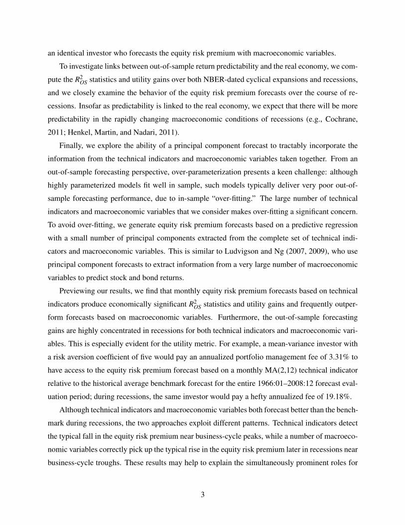
an identical investor who forecasts the equity risk premium with macroeconomic variables.
To investigate links between out-of-sample return predictability and the real economy, we com-
pute the R2OS statistics and utility gains over both NBER-dated cyclical expansions and recessions,
and we closely examine the behavior of the equity risk premium forecasts over the course of re-
cessions. Insofar as predictability is linked to the real economy, we expect that there will be more
predictability in the rapidly changing macroeconomic conditions of recessions (e.g., Cochrane,
2011; Henkel, Martin, and Nadari, 2011).
Finally, we explore the ability of a principal component forecast to tractably incorporate the
information from the technical indicators and macroeconomic variables taken together. From an
out-of-sample forecasting perspective, over-parameterization presents a keen challenge: although
highly parameterized models fit well in sample, such models typically deliver very poor out-of-
sample forecasting performance, due to in-sample “over-fitting.” The large number of technical
indicators and macroeconomic variables that we consider makes over-fitting a significant concern.
To avoid over-fitting, we generate equity risk premium forecasts based on a predictive regression
with a small number of principal components extracted from the complete set of technical indi-
cators and macroeconomic variables. This is similar to Ludvigson and Ng (2007, 2009), who use
principal component forecasts to extract information from a very large number of macroeconomic
variables to predict stock and bond returns.
Previewing our results, we find that monthly equity risk premium forecasts based on technical
indicators produce economically significant R2OS statistics and utility gains and frequently outper-
form forecasts based on macroeconomic variables. Furthermore, the out-of-sample forecasting
gains are highly concentrated in recessions for both technical indicators and macroeconomic vari-
ables. This is especially evident for the utility metric. For example, a mean-variance investor with
a risk aversion coefficient of five would pay an annualized portfolio management fee of 3.31% to
have access to the equity risk premium forecast based on a monthly MA(2,12) technical indicator
relative to the historical average benchmark forecast for the entire 1966:01–2008:12 forecast eval-
uation period; during recessions, the same investor would pay a hefty annualized fee of 19.18%.
Although technical indicators and macroeconomic variables both forecast better than the bench-
mark during recessions, the two approaches exploit different patterns. Technical indicators detect
the typical fall in the equity risk premium near business-cycle peaks, while a number of macroeco-
nomic variables correctly pick up the typical rise in the equity risk premium later in recessions near
business-cycle troughs. These results may help to explain the simultaneously prominent roles for
3

macroeconomic variables in the academic literature and technical indicators among practitioners.
Both approaches seem useful for predicting returns, and they appear to complement each other.
We also show that the principal component forecast, which incorporates information from both
technical indicators and macroeconomic variables, outperforms any of the forecasts based on in-
dividual technical indictors or macroeconomic variables in terms of both the R2OS and utility gain
metrics. Furthermore, the principal component forecast produces larger out-of-sample gains than
the recently proposed methods of Rapach, Strauss, and Zhou (2010) and Ferreira and Santa-Clara
(2011). There is thus considerable value in pooling the information in technical indicators and
macroeconomic variables. Like forecasts based on technical indicators, the principal component
forecast is typically well below the historical average forecast near cyclical peaks; like the best-
performing forecasts based on macroeconomic variables, the principal component forecast is typ-
ically well above the historical average near cyclical troughs. The principal component forecast
thus utilizes important information from both technical indicators and macroeconomic variables.
Overall, our findings suggest that technical indicators are at least as useful as macroeconomic
variables and capture additional relevant information for forecasting the equity risk premium.
Hence, empirical asset pricing may need to pay more attention to technical indicators in explaining
asset returns. Furthermore, our results raise the open question of why technical indicators predict
the equity risk premium. Existing asset pricing models typically ignore the information investors
have about technical indicators, so that our study calls for new asset pricing models that can im-
prove our understanding of the role of technical indicators and their equilibrium pricing impacts.2
The remainder of the paper is organized as follows. Section 2 outlines the construction of
equity risk premium forecasts based on macroeconomic variables and technical indicators, as well
as the forecast evaluation criteria. Section 3 reports out-of-sample test results. Section 4 analyzes
the principal component forecast. Section 5 concludes.
2Behavioral models offer potential explanations for the predictive ability of technical indicators, especially duringrecessions, although these models have not typically been formalized for technical indicators per se. Hong and Stein(1999) and Hong, Lim, and Stein (2000) provide both theory and empirical evidence on the slow transmission of badnews in financial markets. Recessions are presumably associated with large adverse macroeconomic news shocks,which may take longer to be fully incorporated into stock prices. As a result, the market will exhibit stronger trendingpatterns during recessions, creating greater scope for trend-based technical indicators to forecast equity prices. Con-sistent with this is the disposition effect—investors tend to hold losers too long and sell winners too early (Odean,1998). During the early stages of recessions, there are more share price declines and hence more losers; this impliesthat the disposition effect is stronger in recessions, thereby reinforcing the stronger trend.
4

2. Econometric methodology
This section describes the construction and evaluation of out-of-sample equity risk premium
forecasts based on macroeconomic variables and technical indicators.
2.1. Forecast construction
The conventional framework for analyzing equity risk premium predictability based on macroe-
conomic variables is the following predictive regression model:
rt+1 = αi +βixi,t + εi,t+1, (1)
where rt+1 is the return on a broad stock market index in excess of the risk-free rate from period
t to t + 1, xi,t is a predictor (e.g., the dividend yield), and εi,t+1 is a zero-mean disturbance term.
Following Campbell and Thompson (2008) and Goyal and Welch (2003, 2008), we generate an
out-of-sample forecast of rt+1 based on (1) and information through period t as
ri,t+1 = αi,t + βi,txi,t , (2)
where αi,t and βi,t are the ordinary least squares (OLS) estimates of αi and βi, respectively, in
(1) computed by regressing {rk}tk=2 on a constant and {xi,k}t−1k=1. Dividing the total sample of
T observations into q1 in-sample and q2 out-of-sample observations, where T = q1 + q2, we can
calculate a series of out-of-sample equity risk premium forecasts based on xi,t over the last q2
observations: {ri,t+1}T−1t=q1
.3 The historical average of the equity risk premium, rt+1 =(1/t)∑tk=1 rk,
is a natural benchmark forecast corresponding to the constant expected excess return model (βi =
0 in (1)). Goyal and Welch (2003, 2008) show that rt+1 is a stringent benchmark: predictive
regression forecasts based on macroeconomic variables frequently fail to outperform the historical
average forecast in out-of-sample tests.
Campbell and Thompson (2008) demonstrate that parameter and forecast sign restrictions im-
prove individual forecasts based on macroeconomic variables, allowing them to more consistently
outperform the historical average equity risk premium forecast. For example, theory often indicates
the expected sign of βi in (1), so that we set βi = 0 when forming a forecast if the estimated slope
3Observe that the forecasts are generated using a recursive (i.e., expanding) window for estimating αi and βi in (1).Forecasts could also be generated using a rolling window (which drops earlier observations as additional observationsbecome available) in recognition of potential structural instability. Pesaran and Timmermann (2007) and Clark andMcCracken (2009), however, show that the optimal estimation window for a quadratic loss function can include pre-break data due to the familiar bias-efficiency tradeoff. We use recursive estimation windows in Section 3, although weobtain similar results using rolling estimation windows of various sizes.
5

coefficient does not have the expected sign. Campbell and Thompson (2008) also suggest setting
the equity risk premium forecast to zero if the predictive regression forecast is negative, since risk
considerations typically imply a positive expected equity risk premium based on macroeconomic
variables.
In addition to macroeconomic variables, we consider three popular types of technical indica-
tors. The first is an MA rule that, in its simplest form, generates a buy or sell signal (St = 1 or
St = 0, respectively) at the end of period t by comparing two moving averages:
St =
{1 if MAs,t ≥MAl,t0 if MAs,t < MAl,t
, (3)
where
MA j,t = (1/ j)j−1
∑i=0
Pt−i for j = s, l, (4)
Pt is the level of a stock price index, and s (l) is the length of the short (long) MA (s < l). We
denote the MA rule with MA lengths s and l as MA(s, l). Intuitively, the MA rule is designed to
detect changes in stock price trends. For example, when prices have recently been falling, the short
MA will tend to be lower than the long MA. If prices begin trending upward, then the short MA
tends to increase faster than the long MA, eventually exceeding the long MA and generating a buy
signal. In Section 3, we analyze monthly MA rules with s = 1,2,3 and l = 9,12.
The second type of technical indicator we consider is based on momentum. A simple momen-
tum rule generates the following signal:
St =
{1 if Pt ≥ Pt−m0 if Pt < Pt−m
. (5)
Intuitively, a current stock price that is higher than its level m periods ago indicates “positive”
momentum and relatively high expected excess returns, which generates a buy signal. We denote
the momentum rule that compares Pt to Pt−m as MOM(m), and we compute monthly signals for
m = 9,12 in Section 3.
Technical analysts frequently use volume data in conjunction with past prices to identify market
trends. In light of this, the final type of technical indicator we consider employs “on-balance”
volume (e.g., Granville, 1963). We first define
OBVt =t
∑k=1
VOLkDk, (6)
6
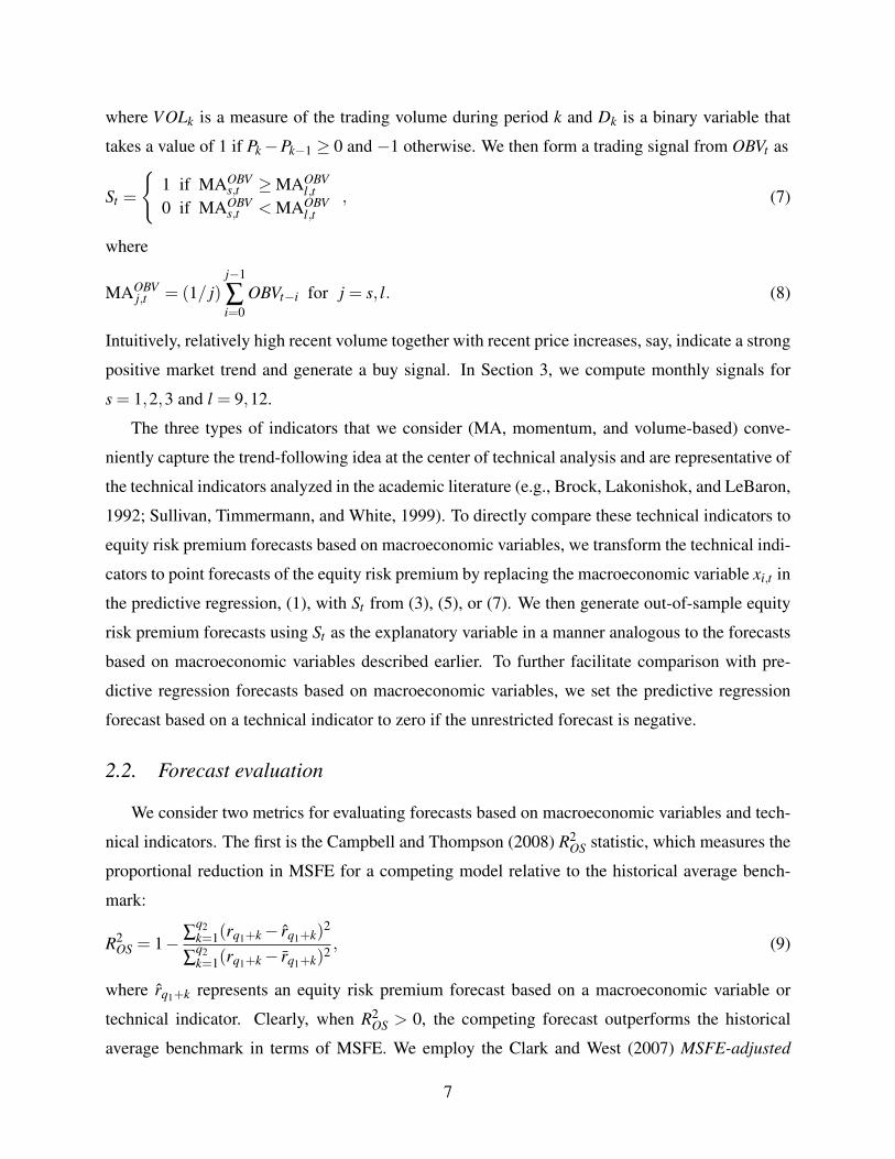
where VOLk is a measure of the trading volume during period k and Dk is a binary variable that
takes a value of 1 if Pk−Pk−1 ≥ 0 and −1 otherwise. We then form a trading signal from OBVt as
St =
{1 if MAOBV
s,t ≥MAOBVl,t
0 if MAOBVs,t < MAOBV
l,t, (7)
where
MAOBVj,t = (1/ j)
j−1
∑i=0
OBVt−i for j = s, l. (8)
Intuitively, relatively high recent volume together with recent price increases, say, indicate a strong
positive market trend and generate a buy signal. In Section 3, we compute monthly signals for
s = 1,2,3 and l = 9,12.
The three types of indicators that we consider (MA, momentum, and volume-based) conve-
niently capture the trend-following idea at the center of technical analysis and are representative of
the technical indicators analyzed in the academic literature (e.g., Brock, Lakonishok, and LeBaron,
1992; Sullivan, Timmermann, and White, 1999). To directly compare these technical indicators to
equity risk premium forecasts based on macroeconomic variables, we transform the technical indi-
cators to point forecasts of the equity risk premium by replacing the macroeconomic variable xi,t in
the predictive regression, (1), with St from (3), (5), or (7). We then generate out-of-sample equity
risk premium forecasts using St as the explanatory variable in a manner analogous to the forecasts
based on macroeconomic variables described earlier. To further facilitate comparison with pre-
dictive regression forecasts based on macroeconomic variables, we set the predictive regression
forecast based on a technical indicator to zero if the unrestricted forecast is negative.
2.2. Forecast evaluation
We consider two metrics for evaluating forecasts based on macroeconomic variables and tech-
nical indicators. The first is the Campbell and Thompson (2008) R2OS statistic, which measures the
proportional reduction in MSFE for a competing model relative to the historical average bench-
mark:
R2OS = 1− ∑
q2k=1(rq1+k− rq1+k)
2
∑q2k=1(rq1+k− rq1+k)2 , (9)
where rq1+k represents an equity risk premium forecast based on a macroeconomic variable or
technical indicator. Clearly, when R2OS > 0, the competing forecast outperforms the historical
average benchmark in terms of MSFE. We employ the Clark and West (2007) MSFE-adjusted
7

statistic to test the null hypothesis that the competing model MSFE is greater than or equal to the
historical average MSFE against the one-sided alternative hypothesis that the competing forecast
has a lower MSFE, corresponding to H0 : R2OS ≤ 0 against HA : R2
OS > 0. Clark and West (2007)
develop the MSFE-adjusted statistic by modifying the familiar Diebold and Mariano (1995) and
West (1996) statistic so that it has a standard normal asymptotic distribution when comparing
forecasts from nested models. Comparing the forecasts based on macroeconomic variables or
technical indicators with the historical average forecast entails comparing nested models, since
setting βi = 0 in (1) yields the constant expected excess return model.4
R2OS statistics are typically small for equity risk premium forecasts, since aggregate excess
returns inherently contain a large unpredictable component, but a relatively small R2OS statistic can
still signal economically important gains for an investor (Kandel and Stambaugh, 1996; Xu, 2004;
Campbell and Thompson, 2008). From an asset allocation perspective, however, the utility gain
itself is the key metric. As a second metric for evaluating forecasts, we thus compute realized
utility gains for a mean-variance investor who optimally allocates across stocks and risk-free bills,
as in, among others, Marquering and Verbeek (2004) and Campbell and Thompson (2008). As
discussed in the introduction, this procedure addresses the weakness of many existing studies of
technical indicators that fail to incorporate the degree of risk aversion into the asset allocation
decision.
In particular, we compute the average utility for a mean-variance investor with risk aversion
coefficient of five who monthly allocates between stocks and risk-free bills using an equity risk
premium forecast based on a macroeconomic variable or technical indicator. Following Camp-
bell and Thompson (2008), we assume that the investor uses a five-year moving window of past
monthly returns to estimate the variance of the equity risk premium, and we constrain the equity
weight in the portfolio to lie between 0% and 150%. We then calculate the average utility for the
same investor using the historical average forecast of the equity risk premium. The utility gain is
the difference between the two average utilities. We multiply this difference by 1200, so that it can
be interpreted as the annual percentage portfolio management fee that an investor would be willing
to pay to have access to the equity risk premium forecast based on a macroeconomic variable or
technical indicator relative to the historical average forecast.
4While the Diebold and Mariano (1995) and West (1996) statistic has a standard normal asymptotic distributionwhen comparing forecasts from non-nested models, Clark and McCracken (2001) and McCracken (2007) show that ithas a complicated non-standard distribution when comparing forecasts from nested models. The non-standard distri-bution can lead the Diebold and Mariano (1995) and West (1996) statistic to be severely undersized when comparingforecasts from nested models, thereby substantially reducing power.
8

3. Empirical results
This section describes the data and reports the out-of-sample test results for the R2OS statistics
and average utility gains.
3.1. Data
Our monthly data span 1927:01–2008:12. The data are from Amit Goyal’s web page, which
provides updated data from Goyal and Welch (2008).5 The aggregate market return is the continu-
ously compounded return on the S&P 500 (including dividends), and the equity risk premium is the
difference between the aggregate market return and the log return on a risk-free bill. The follow-
ing 14 macroeconomic variables, which are well representative of the literature (Goyal and Welch,
2008), constitute the set of macroeconomic variables used to forecast the equity risk premium:
1. Dividend-price ratio (log), DP: log of a twelve-month moving sum of dividends paid on the
S&P 500 index minus the log of stock prices (S&P 500 index).
2. Dividend yield (log), DY: log of a twelve-month moving sum of dividends minus the log of
lagged stock prices.
3. Earnings-price ratio (log), EP: log of a twelve-month moving sum of earnings on the S&P
500 index minus the log of stock prices.
4. Dividend-payout ratio (log), DE: log of a twelve-month moving sum of dividends minus the
log of a twelve-month moving sum of earnings.
5. Stock variance, SVAR: monthly sum of squared daily returns on the S&P 500 index.
6. Book-to-market ratio, BM: book-to-market value ratio for the Dow Jones Industrial Average.
7. Net equity expansion, NTIS: ratio of a twelve-month moving sum of net equity issues by
NYSE-listed stocks to the total end-of-year market capitalization of NYSE stocks.
8. Treasury bill rate, TBL: interest rate on a three-month Treasury bill (secondary market).
9. Long-term yield, LTY: long-term government bond yield.
10. Long-term return, LTR: return on long-term government bonds.
5The data are available at http://www.hec.unil.ch/agoyal/.
9
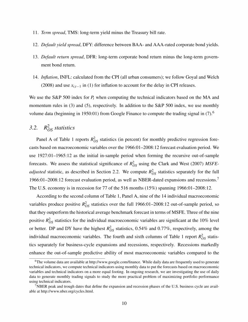
11. Term spread, TMS: long-term yield minus the Treasury bill rate.
12. Default yield spread, DFY: difference between BAA- and AAA-rated corporate bond yields.
13. Default return spread, DFR: long-term corporate bond return minus the long-term govern-
ment bond return.
14. Inflation, INFL: calculated from the CPI (all urban consumers); we follow Goyal and Welch
(2008) and use xi,t−1 in (1) for inflation to account for the delay in CPI releases.
We use the S&P 500 index for Pt when computing the technical indicators based on the MA and
momentum rules in (3) and (5), respectively. In addition to the S&P 500 index, we use monthly
volume data (beginning in 1950:01) from Google Finance to compute the trading signal in (7).6
3.2. R2OS statistics
Panel A of Table 1 reports R2OS statistics (in percent) for monthly predictive regression fore-
casts based on macroeconomic variables over the 1966:01–2008:12 forecast evaluation period. We
use 1927:01–1965:12 as the initial in-sample period when forming the recursive out-of-sample
forecasts. We assess the statistical significance of R2OS using the Clark and West (2007) MSFE-
adjusted statistic, as described in Section 2.2. We compute R2OS statistics separately for the full
1966:01–2008:12 forecast evaluation period, as well as NBER-dated expansions and recessions.7
The U.S. economy is in recession for 77 of the 516 months (15%) spanning 1966:01–2008:12.
According to the second column of Table 1, Panel A, nine of the 14 individual macroeconomic
variables produce positive R2OS statistics over the full 1966:01–2008:12 out-of-sample period, so
that they outperform the historical average benchmark forecast in terms of MSFE. Three of the nine
positive R2OS statistics for the individual macroeconomic variables are significant at the 10% level
or better. DP and DY have the highest R2OS statistics, 0.54% and 0.77%, respectively, among the
individual macroeconomic variables. The fourth and sixth columns of Table 1 report R2OS statis-
tics separately for business-cycle expansions and recessions, respectively. Recessions markedly
enhance the out-of-sample predictive ability of most macroeconomic variables compared to the
6The volume data are available at http://www.google.com/finance. While daily data are frequently used to generatetechnical indicators, we compute technical indicators using monthly data to put the forecasts based on macroeconomicvariables and technical indicators on a more equal footing. In ongoing research, we are investigating the use of dailydata to generate monthly trading signals to study the more practical problem of maximizing portfolio performanceusing technical indicators.
7NBER peak and trough dates that define the expansion and recession phases of the U.S. business cycle are avail-able at http://www.nber.org/cycles.html.
10

historical average. For example, the predictive ability of DP and DY is highly concentrated in
recessions: the R2OS statistics for DP (DY) are−0.10% and 2.06% (−0.20% and 3.06%) during ex-
pansions and recessions, respectively. The R2OS statistics for DP, DY, LTR, and TMS are significant
at the 10% level during recessions, despite the reduced number of available observations; the R2OS
for NTIS (0.01%) is the only statistic that is significant during expansions for the macroeconomic
variables.
To illustrate how equity risk premium forecasts vary over the business cycle, Figure 1 graphs
predictive regression forecasts based on individual macroeconomic variables, along with the his-
torical average benchmark. The vertical bars in the figure depict NBER-dated recessions. Many
of the individual predictive regression forecasts—especially those that perform the best during
recessions, such as DP, DY, and TMS—often increase substantially above the historical average
forecast over the course of recessions, reaching distinct local maxima near cyclical troughs. This
is particularly evident during more severe recessions, such as the mid 1970s and early 1980s.
The countercyclical fluctuations in equity risk premium forecasts in Figure 1 are similar to the
countercyclical fluctuations in in-sample expected equity risk premium estimates reported in, for
example, Fama and French (1989), Ferson and Harvey (1991), Whitelaw (1994), Harvey (2001),
and Lettau and Ludvigson (2009). The fifth and seventh columns of Table 1, Panel A show that the
average equity risk premium forecast is higher during recessions than expansions for a number of
macroeconomic variables, including DP and DY.
Figure 2 provides a time-series perspective on the out-of-sample predictive ability of macroeco-
nomic variables over the business cycle. The figure portrays the cumulative differences in squared
forecast errors between the historical average forecast and forecasts based on individual macroe-
conomic variables.8 A segment of the curve that is higher (lower) at its end point relative to its
initial point indicates that the competing forecast outperforms (underperforms) the historical av-
erage forecast in terms of MSFE over the period corresponding to the segment. The curves are
predominantly positively sloped—sometimes quite steeply—during many recessions in Figure 2
(with the notable exception of NTIS); outside of recessions, the curves are often flat or negatively
sloped. Overall, Figure 2 provides further evidence of the enhanced predictive power of macroe-
conomic variables during recessions.
We turn next to the forecasting performance of the technical indicators in Table 1, Panel B. For
the MA and momentum indicators in (3) and (5), respectively, we use data for 1927:12–1965:12
8Goyal and Welch (2003, 2008) employ this device to assess the consistency of out-of-sample predictive ability.
11

or 1928:01–1965:12 as the initial in-sample period to estimate the predictive regression model that
transforms the trading signals to point forecasts.9 Data availability limits the starting date for the
volume rules’ in-sample period to 1950:12.10 The second column of Table 1, Panel B shows that
twelve of the 14 individual technical forecasts have positive R2OS statistics for 1966:01–2008:12,
so that they outperform the historical average forecast according to the MSFE metric. Eight of the
twelve positive R2OS statistics are significant at conventional levels. Comparing the results in Panels
A and B of Table 1, equity risk premium forecasts based on technical indicators generally provide
more sizable out-of-sample gains than forecasts based on macroeconomic variables.
The fourth and sixth columns of Table 1, Panel B show even starker differences in forecasting
performance across business-cycle phases for the forecasts based on technical indicators in Panel
B compared to the forecasts based on macroeconomic variables in Panel A. Eleven of the 14
individual technical forecasts exhibit negative R2OS statistics during expansions, while all forecasts
have positive R2OS statistics during recessions; twelve of the positive statistics during recessions are
significant at conventional levels. Moreover, the R2OS statistics for the technical forecasts are quite
sizable during recessions, with many ranging from over 1% to close to 4%.
Figure 3 shows that the technical forecasts almost always drop below the historical average
forecast—often substantially so—throughout recessions. There are also expansionary episodes
where some of the technical forecasts frequently fall below the historical average forecast. The
fourth column of Table 1, Panel B indicates that these declines detract from the accuracy of these
technical forecasts during expansions. The fifth and seventh columns of Panel B show that the
average technical forecasts of the equity risk premium are uniformly lower during recessions than
expansions.
Analogous to Figure 2, Figure 4 graphs the cumulative differences in squared forecast errors
between the historical average forecast and technical forecasts. The positive slopes of the curves
during recessions in Figure 4 show that most of the technical forecasts consistently produce out-of-
sample gains during these periods. But the curves are almost always flat or negatively sloped for
expansions, so that out-of-sample gains are nearly limited to recessions. Taken together, the results
in Table 1 and Figures 2 and 4 highlight the relevance of business-cycle fluctuations for equity risk
premium predictability using either macroeconomic variables or technical indicators.
9These starting dates allow for the lags necessary to compute the initial MA or momentum signal in (3) or (5).10This starting date for the volume rules’ in-sample period motivates our selection of 1966:01 as the start of the
forecast evaluation period, since this provides us with approximately 15 years of data for estimating the predictiveregression parameters used to compute the initial forecast based on a volume rule.
12

3.3. Utility gains
Table 2 reports average utility gains, in annualized percent, for a mean-variance investor with
risk aversion coefficient of five who allocates monthly across stocks and risk-free bills using equity
risk premium forecasts derived from macroeconomic variables (Panel A) or technical indicators
(Panel B). The results in Panel A indicate that forecasts based on macroeconomic variables often
produce sizable utility gains vis-a-vis the historical average benchmark. The utility gain is above
0.75% for five of the individual macroeconomic variables in the second column, so that the investor
would be willing to pay an annual management fee of 75 basis points or more to have access to
forecasts based on macroeconomic variables relative to the historical average forecast. Similar to
Table 1, the out-of-sample gains are concentrated in recessions. Consider, for example, DY, which
generates the largest utility gain (2.22%) for the full 1966:01–2008:12 forecast evaluation period.
The utility gain is negative (−0.06%) during expansions, while it is a very sizable 14.85% during
recessions. DP, LTY, LTR, and DFR also provide utility gains above 5% during recessions.
Figure 5 portrays the equity portfolio weights computed using equity risk premium forecasts
based on macroeconomic variables and historical average forecasts. Because the investor uses the
same volatility forecast for all of the portfolio allocations, only the equity risk premium forecasts
produce differences in the equity weights. Figure 5 shows that the equity weight computed using
the historical average forecast is procyclical, which, given that the historical average forecast of
the equity risk premium is relatively smooth, primarily reflects countercyclical changes in expected
volatility.11 The equity weights based on macroeconomic variables often deviate substantially from
the equity weight based on the historical average, with a tendency for the weights computed using
macroeconomic variables to lie below the historical average weight during expansions and move
closer to or above the historical average weight during recessions. Panel A of Table 2 indicates that
these deviations create significant utility gains for our mean-variance investor, especially during
recessions.
The second column of Table 2, Panel B shows that all 14 of the utility gains for forecasts based
on technical indicators are positive for the full 1966:01–2008:12 out-of-sample period. Eleven
of the individual technical forecasts provide utility gains above 1%, with the MA(2,12) forecast
generating the largest gain (3.31%). Comparing the fourth and sixth columns, the utility gains are
substantially higher and more consistent during recessions than during expansions. The MA(1,9)
11French, Schwert, and Stambaugh (1987), Schwert (1989, 1990), Whitelaw (1994), Harvey (2001), Ludvigson andNg (2007), Lundblad (2007), and Lettau and Ludvigson (2009), among others, also find evidence of countercyclicalexpected volatility using alternative volatility estimators.
13

forecast provides a leading example: the utility gain is negative during expansions (−0.99%),
while it jumps to 19.82% during recessions. In all, twelve of the individual technical forecasts
produce utility gains above 10% during recessions. The fifth and seventh columns reveal that
the average equity weight is substantially lower during recessions than expansions for all of the
technical forecasts.
Figure 6 further illustrates that technical forecast weights tend to decrease during recessions,
dropping below the weight based on the historical average forecast during cyclical downturns.
Again recalling that the investor uses the same rolling-window variance estimator for all portfolio
allocations, these declining weights reflect decreases in the technical forecasts during recessions,
as discussed in the context of Figure 3.
Overall, Table 2 shows that equity risk premium forecasts based on both macroeconomic vari-
ables and technical indicators usually generate sizable utility gains, especially during recessions,
highlighting the economic significance of equity risk premium predictability using either approach.
Comparing Panels A and B of Table 2, forecasts based on technical indicators typically provide
larger utility gains than forecasts based on macroeconomic variables over the full 1966:01–2008:12
forecast evaluation period and during recessions.
3.4. A closer look at forecast behavior near cyclical peaks and troughs
Tables 1 and 2 and Figures 1–6 present somewhat of a puzzle. Out-of-sample gains are typi-
cally concentrated in recessions for equity risk premium forecasts based on both macroeconomic
variables and technical indicators. However, equity risk premium forecasts based on macroeco-
nomic variables often increase during recessions, while forecasts based on technical indicators are
usually substantially lower during recessions than expansions. Despite the apparent differences in
the behavior of the two types of forecasts during recessions, the out-of-sample gains are concen-
trated in cyclical downturns for both approaches. Why?
We investigate this issue by examining the behavior of the actual equity risk premium and
forecasts around cyclical peaks and troughs, which define the beginnings and ends of recessions,
respectively. We first estimate the following regression model around cyclical peaks:
rt− rt = aP +4
∑k=−2
bP,kIPk,t + eP,t , (10)
where IPk,t is an indicator variable that takes a value of unity k months after an NBER-dated peak
and zero otherwise. The estimated bP,k coefficients measure the incremental change in the average
14

difference between the realized equity risk premium and historical average forecast k months after
a cyclical peak. We then estimate a corresponding model that replaces the actual equity risk pre-
mium, rt , with an equity risk premium forecast based on a macroeconomic variable or technical
indicator:
rt− rt = aP +4
∑k=−2
bP,kIPk,t + eP,t . (11)
The slope coefficients describe the incremental change in the average difference between a forecast
based on a macroeconomic variable or technical indicator relative to the historical average forecast
k periods after a cyclical peak. Similarly, we measure the incremental change in the average
behavior of the realized equity risk premium and the forecasts around cyclical troughs:
rt− r = aT +∑2k=−4 bT,kIT
k,t + eT,t , (12)
rt− rt = aT +∑2k=−4 bT,kIT
k,t + eT,t , (13)
where ITk,t is an indicator variable equal to unity k months after an NBER-dated trough and zero
otherwise.
The top-left panel of Figure 7 graphs OLS slope coefficient estimates (in percent) and 90%
confidence bands for (10), and the remaining panels depict corresponding estimates for (11) based
on individual macroeconomic variables. The top-left panel shows that the actual equity risk pre-
mium tends to move significantly below the historical average forecast one month before through
two months after a cyclical peak. The remaining panels in Figure 7 indicate that most macroeco-
nomic variables fail to pick up this decline in the equity risk premium early in recessions. Only the
LTR, TMS, and INFL forecasts are significantly below the historical average forecast for any of
the months early in recessions when the equity risk premium itself is lower than average, although
the size of the decline in the INFL forecast is very small. The TMS forecast does the best job
of matching the lower-than-average actual equity risk premium for the month before through two
months after a peak. However, the TMS forecast is also significantly lower than the historical aver-
age forecast two months before and three and four months after a peak, unlike the actual equity risk
premium. Overall, Figure 7 suggests that equity risk premium forecasts based on macroeconomic
variables fail to detect the decline in the equity risk premium near cyclical peaks.
How do the equity risk premium forecasts based on technical indicators behave near cyclical
peaks? The top-left panel of Figure 8 again shows estimates for (10), while the other panels graph
estimates for (11) based on individual technical indicators. Figure 8 reveals that most of the tech-
nical forecasts move substantially below the historical average forecast in the months immediately
15

following a cyclical peak, in accord with the behavior of the actual equity risk premium. Given
that the actual equity risk premium moves substantially below average in the month before and
month of a cyclical peak, it is not surprising that technical forecasts are nearly all lower than the
historical average in the first two months after a peak, since the technical forecasts are based on
signals that recognize trends in equity prices. This trend-following behavior early in recessions
apparently helps to generate the sizable out-of-sample gains during recessions for the technical
forecasts in Tables 1 and 2. The forecasts based on technical indicators in Figure 8 tend to remain
well below the historical average for too long after a peak, however.
Figures 9 and 10 depict estimates of the slope coefficients in (12) and (13) for forecasts based
on macroeconomic variables and technical indicators, respectively. The top-left panel in each
figure shows that the actual equity risk premium moves significantly above the historical average
forecast in the third and second months before a cyclical trough, so that the equity risk premium
is higher than usual in the late stages of recessions. Figure 9 indicates that many of the forecasts
based on macroeconomic variables, particularly those based on DP, DY, BM, and LTR, are also
significantly higher than the historical average forecast in the third and second months before a
trough. The TMS forecast is also well above the historical average in the later stages of recessions,
although by less than the previously mentioned macroeconomic variables. The ability of many
of the forecasts based on macroeconomic variables to match the higher-than-average equity risk
premium late in recessions helps to account for the sizable out-of-sample gains during recessions
for forecasts based on macroeconomic variables in Tables 1 and 2.
Figure 10 shows that forecasts based on technical indicators typically start low but rise quickly
late in recessions, in contrast to the pattern in the actual equity risk premium. The out-of-sample
gains for the technical forecasts during recessions in Tables 1 and 2 thus occur despite the relatively
poor performance of technical forecasts late in recessions. While the trend-following technical
forecasts detect the decrease in the actual equity risk premium early in recessions (see Figure 8),
they do not recognize the unusually high actual equity risk premium late in recessions.
In summary, Figures 7–10 paint the following nuanced picture with respect to the sizable out-
of-sample gains during recessions in Tables 1 and 2. Macroeconomic variables typically fail to
detect the decline in the actual equity risk premium early in recessions, but generally do detect
the increase in the actual equity risk premium late in recessions. Technical indicators exhibit the
opposite pattern: they pick up the decline in the actual premium early in recessions, but fail to
match the unusually high premium late in recessions. Although both types of forecasts generate
16
substantial out-of-sample gains during recessions, they capture different aspects of equity risk
premium fluctuations during cyclical downturns. This suggests that fundamental and technical
analysis provide complementary approaches to out-of-sample equity risk premium predictability.
We explore this complementarity further in the next section.
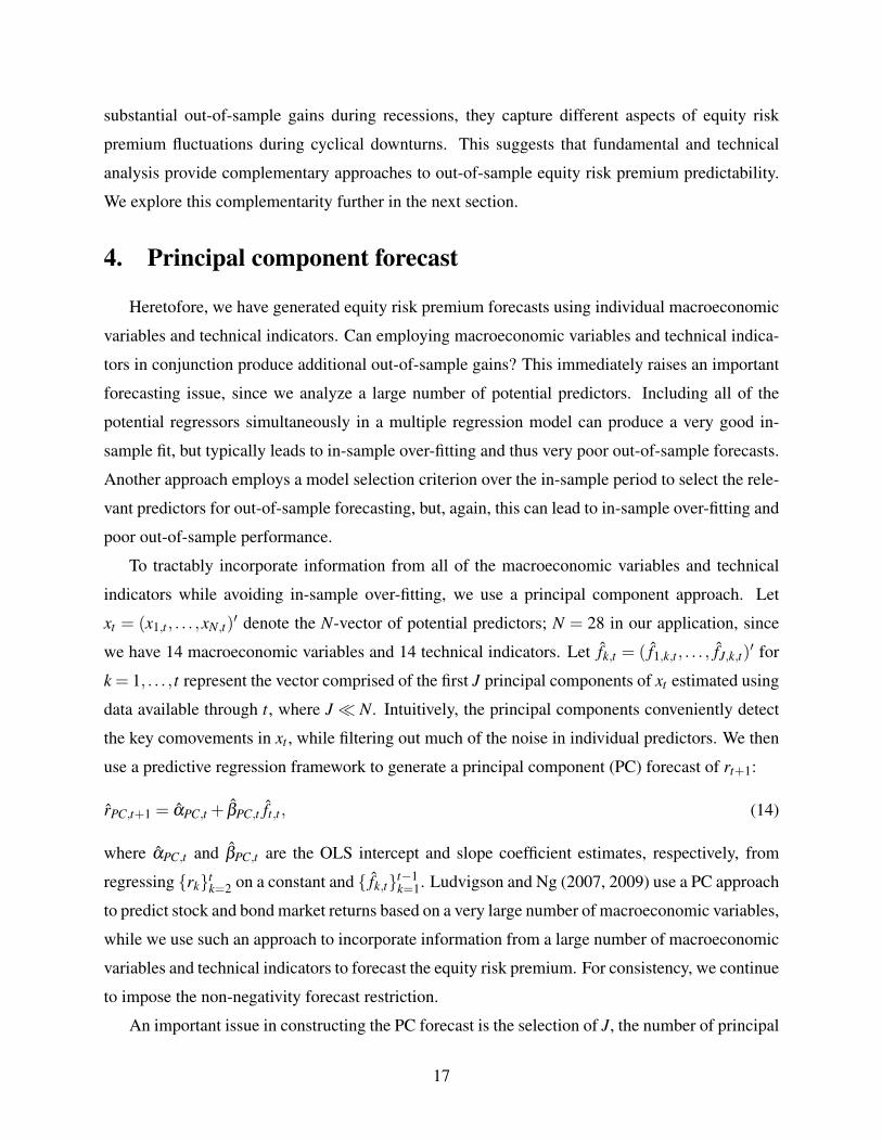
4. Principal component forecast
Heretofore, we have generated equity risk premium forecasts using individual macroeconomic
variables and technical indicators. Can employing macroeconomic variables and technical indica-
tors in conjunction produce additional out-of-sample gains? This immediately raises an important
forecasting issue, since we analyze a large number of potential predictors. Including all of the
potential regressors simultaneously in a multiple regression model can produce a very good in-
sample fit, but typically leads to in-sample over-fitting and thus very poor out-of-sample forecasts.
Another approach employs a model selection criterion over the in-sample period to select the rele-
vant predictors for out-of-sample forecasting, but, again, this can lead to in-sample over-fitting and
poor out-of-sample performance.
To tractably incorporate information from all of the macroeconomic variables and technical
indicators while avoiding in-sample over-fitting, we use a principal component approach. Let
xt = (x1,t , . . . ,xN,t)′ denote the N-vector of potential predictors; N = 28 in our application, since
we have 14 macroeconomic variables and 14 technical indicators. Let fk,t = ( f1,k,t , . . . , fJ,k,t)′ for
k = 1, . . . , t represent the vector comprised of the first J principal components of xt estimated using
data available through t, where J� N. Intuitively, the principal components conveniently detect
the key comovements in xt , while filtering out much of the noise in individual predictors. We then
use a predictive regression framework to generate a principal component (PC) forecast of rt+1:
rPC,t+1 = αPC,t + βPC,t ft,t , (14)
where αPC,t and βPC,t are the OLS intercept and slope coefficient estimates, respectively, from
regressing {rk}tk=2 on a constant and { fk,t}t−1k=1. Ludvigson and Ng (2007, 2009) use a PC approach
to predict stock and bond market returns based on a very large number of macroeconomic variables,
while we use such an approach to incorporate information from a large number of macroeconomic
variables and technical indicators to forecast the equity risk premium. For consistency, we continue
to impose the non-negativity forecast restriction.
An important issue in constructing the PC forecast is the selection of J, the number of principal
17

components to include in (14). We need J to be relatively small to avoid an overly parameterized
model; at the same time, we do not want to include too few principal components, thereby ne-
glecting important information in xt . We select J using the Onatski (2009) ED algorithm. This
algorithm displays good properties for selecting the true number of factors in approximate factor
models for sample sizes near ours in simulations in Onatski (2009). The ED algorithm typically
selects J = 3 when forming recursive PC forecasts using the 14 macroeconomic variables and 14
technical indicators.
Panel A of Table 3 reports R2OS statistics for the PC forecast for the full 1966:01–2008:12 fore-
cast evaluation period and separately during expansions and recessions. The R2OS statistic is 1.66%
for the full period, which is significant at the 1% level and well above all of the corresponding R2OS
statistics for the forecasts based on individual macroeconomic variables and technical indicators
in Table 1. Similar to the results in Table 1, the PC forecast R2OS is substantially higher during re-
cessions (4.37%, significant at the 1% level) than expansions (0.50%, significant at the 10% level).
The R2OS statistics for the PC forecast during expansions and recessions are higher than each of the
corresponding R2OS statistics in Table 1.
The top panel of Figure 11 depicts the time series of PC equity risk premium forecasts. The
PC forecast exhibits a close connection to the business cycle. In particular, the PC forecast is
typically well below the historical average forecast near cyclical peaks. At the same time, the
PC forecast moves well above the historical average forecast near cyclical troughs corresponding
to more severe recessions. This cyclical pattern in the PC forecast indicates that it incorporates
the relevant information from both macroeconomic variables and technical indicators that enhance
equity risk premium predictability, as discussed in Section 3.
Analogous to Figures 2 and 4, the middle panel of Figure 11 graphs the difference in cumulative
squared forecast errors for the historical average forecast relative to the PC forecast. The curve is
predominantly positively sloped throughout the 1966:01–2008:12 period, so that the PC forecast
delivers out-of-sample gains on a consistent basis over time, much more consistently than any of
the forecasts based on individual macroeconomic variables and technical indicators in Figures 2
and 4. The curve is frequently steeply sloped during recessions, again highlighting the importance
of business-cycle fluctuations for equity risk premium predictability.
The PC forecast also generates substantial utility gains from an asset allocation perspective,
as evidenced by Table 3, Panel B. The utility gain is 4.35% for the full 1966:01–2008:12 forecast
evaluation period, which is well above any of the corresponding utility gains for forecasts based
18

on individual macroeconomic variables and technical indicators in Table 2. Continuing the famil-
iar pattern, the utility gains are concentrated during economic contractions, with gains of 1.21%
and 21.97% during expansions and recessions, respectively. The gains during expansions and re-
cessions are again greater than any of the corresponding gains in Table 2. The average equity
weights reported in the last row of Table 2 show that the average equity weight is lower during
recessions vis-a-vis expansions (0.08 and 0.31, respectively). Inspection of the bottom panel of
Figure 11 shows that the average equity weight of 0.08 during recession masks sizable shifts in
asset allocation during recessions: the PC forecast typically leads the investor to move entirely out
of stocks near cyclical peaks and throughout much of the downturn; however, the investor tends to
move aggressively back into stocks late in recessions near cyclical troughs of severe recessions. In
contrast, the historical forecast is much less capable of “timing” the market near recession peaks
and troughs.
“Data snooping” concerns naturally arise when considering a host of potential predictors. To
control for data snooping, we use a modified version of White’s (2000) reality check due to Clark
and McCracken (2010). The Clark and McCracken (2010) reality check is based on a wild fixed-
regressor bootstrap and is appropriate for comparing forecasts from multiple models that all nest
the benchmark model, as in our framework.12 Specifically, we test the null hypothesis that the
MSFE for each of the competing models is greater than or equal to the MSFE for the historical
average benchmark against the alternative hypothesis that at least one of the competing models has
a lower MSFE. This corresponds to a test of H0: R2OS,m ≤ 0 for all m = 1, . . . ,M, where m indexes
a competing model, against HA: R2OS,m > 0 for at least one m. We implement this test using the
Clark and McCracken (2010) maxMSFE-Fm statistic:
maxMSFE-Fm = maxm=1,...,M
q2dm
MSFEm, (15)
where q2 is the size of the forecast evaluation period,
dm = (1/q2)q2
∑k=1
[(rk− rk)
2− (rk− rm,k)2] , (16)
MSFEm = (1/q2)q2
∑k=1
(rk− rm,k)2. (17)
12As Clark and McCracken (2010) emphasize, the asymptotic and finite-sample properties of the non-parametricbootstrap procedures in White’s (2000) reality check (as well as Hansen’s (2005) modified reality check) do not gener-ally apply when comparing forecasts from multiple models that all nest the benchmark model. Clark and McCracken(2010) show that a wild fixed-regressor bootstrap procedure for maximum statistics delivers asymptotically valid crit-ical values. They also find that this bootstrap procedure has good finite-sample properties.
19

In our application, M = 29, corresponding to the 14 forecasts based on individual macroeconomic
variables, 14 forecasts based on individual technical indicators, and the PC forecast. For the
1966:01–2008:12 forecast evaluation period, the maxMSFE-Fm statistic equals 8.70, with a wild
fixed-regressor bootstrap p-value of 4.71%, so that we reject the null hypothesis that none of the
competing models outperforms the historical average benchmark in terms of MSFE at conven-
tional significance levels.13 This reality check indicates that data snooping cannot readily explain
the out-of-sample equity risk premium predictability in Tables 1 and 3.
Finally, we briefly compare the out-of-sample gains from the PC forecast, which incorporates
information from both macroeconomic variables and technical indicators, to two recently proposed
methods for improving out-of-sample equity risk premium forecasts. Rapach, Strauss, and Zhou
(2010) show that a combination forecast delivers consistent out-of-sample gains relative to equity
risk premium forecasts based on individual macroeconomic variables. Using the same approach,
we form a combination forecast as the mean of the forecasts based on the 14 individual macroeco-
nomic variables that we consider. This combination forecast produces an R2OS of 0.63% and utility
gain of 1.36% for the 1966:01–2008:12 forecast evaluation period.14 These values are both well
below the R2OS of 1.66% and utility gain of 4.35% for the PC forecast in Table 3 during this period.
Ferreira and Santa-Clara (2011) develop an intriguing “sum-of-the-parts” (SOP) approach to
forecast the market return. Specifically, they decompose the log market return into the sum of
the growth in the price-earnings ratio, growth in earnings, and the dividend-price ratio. Treating
earnings growth as largely unforecastable and the dividend-price and earnings-price ratios as ap-
proximately random walks, Ferreira and Santa-Clara (2011) propose the SOP equity risk premium
forecast as the sum of a 20-year moving average of earnings growth rates and the current dividend-
price ratio (minus the risk-free rate).15 They show that the SOP forecast outperforms equity risk
premium forecasts based on individual macroeconomic variables over the postwar period, primar-
ily by reducing estimation error. For the 1966:01–2008:12 forecast evaluation period, the SOP
forecast generates an R2OS of 1.19% and utility gain of 2.34%.16 These values are larger than the
corresponding values for any of the individual macroeconomic variables in Tables 1 and 2, as well
as those for the combination forecast. However, the R2OS and utility gain for the SOP forecast are
13The wild fixed-regressor bootstrap used to compute the p-value is described in detail in the appendix.14Rapach, Strauss, and Zhou (2010) report an R2
OS of 3.58% and utility gain of 2.34% for quarterly (instead ofmonthly) equity risk premium forecasts for the 1965:1–2005:4 forecast evaluation period.
15Ferreira and Santa-Clara (2011) focus on forecasting the market return, but note that they obtain similar resultsfor the equity risk premium.
16The R2OS of 1.19% is reasonably near the R2
OS of 1.32% (0.98%) for the market return reported by Ferreira andSanta-Clara (2011) for the 1948:01–2007:12 (1977:01–2007:12) forecast evaluation period.
20

substantially lower than the corresponding values of 1.66% and 4.35% for the PC forecast in Table
3. In short, the ability of the PC forecast to outperform the combination and SOP forecasts further
establishes the relevance of technical indicators for equity risk premium forecasting.
5. Conclusion
We analyze monthly out-of-sample forecasts of the U.S. equity risk premium based on pop-
ular technical indicators in comparison to that of a set of well-known macroeconomic variables
using two out-of-sample metrics: (1) the Campbell and Thompson (2008) R2OS statistic and (2) the
average utility gain for a mean-variance investor who optimally reallocates a monthly portfolio be-
tween equities and risk-free Treasury bills using equity risk premium forecasts based on technical
indicators or macroeconomic variables relative to the historical average benchmark forecast. We
find that technical indicators have statistically and economically significant out-of-sample forecast-
ing power and frequently outperform macroeconomic variables. While both approaches perform
disproportionately well during recessions, a careful analysis of their performance during cyclical
downturns reveals that they exploit very different patterns: technical indicators recognize the typ-
ical drop in the equity risk premium near cyclical peaks; macroeconomic variables identify the
typical increase in the equity risk premium near cyclical troughs. Thus, technical indicators and
macroeconomic variables represent complementary approaches to equity risk premium forecast-
ing.
Building on this complementarity, we generate a principal component equity risk premium
forecast, which incorporates information from all of the technical indicators and macroeconomic
variables taken together. The principal component forecast performs very well, delivering substan-
tially larger out-of-sample gains than any of the forecasts based on individual technical indicators
or macroeconomic variables. These gains stem in large measure from the principal component
forecast’s ability to utilize the complementary information in technical indicators and macroeco-
nomic variables and thus better track the equity risk premium during recessions.
Our results suggest avenues for future research. We show that technical market indicators can
be used in a predictive regression framework to improve equity risk premium forecasts. However,
forecasting the equity risk premium using technical market indicators in this manner is a special
case of employing the information generally available in a broad range of technical indicators.
More sophisticated use of past information has the potential to further improve forecasting power.
A leading example is Cochrane and Piazzesi (2005), who show that a factor formed as a “tent-
21

shaped” linear combination of forward rates has substantial predictor power for U.S. bond risk
premia. While our principal component forecast is in the spirit of this approach, alternative meth-
ods for forming factors based on technical indicators are worth investigating. Given that numerous
empirical studies use various economic variables to explain the cross section of expected asset
returns, it would also be interesting to incorporate technical indicators into this analysis.
Our paper provides empirical evidence calling for the incorporation of past information, espe-
cially technical market indictors, into asset pricing models. Leading asset pricing models, such as
the Campbell and Cochrane (1999) habit-formation and Bansal and Yaron (2004) long-run risks
models, as well as their recent extensions by Bekaert, Engstrom, and Xing (2009) and Bollerslev,
Tauchen, and Zhou (2009), provide theoretical explanations for equity risk premium predictability
based on macroeconomic variables in general equilibrium settings. It is not clear, however, the
extent to which these models can account for the forecasting ability of technical indicators. Do
technical indicators correlate with aggregate risk factors? Alternatively (or additionally), do they
represent behavioral influences or information processing limitations? Given that technical indica-
tors appear to provide useful information for equity risk premium forecasting, these are important
theoretical questions.
22

Appendix: Wild fixed-regressor bootstrap
This appendix outlines the wild fixed-regressor bootstrap used to calculate the p-value for the
maxMSFE-Fm statistic given by (15). We first estimate the constant expected equity risk premium
model, corresponding to the null of no predictability: r = (1/T )∑Tt=1 rt . We next estimate an unre-
stricted model that includes all of the potential predictors as regressors using OLS; denote the OLS
residuals from this model as {ut}Tt=1. We then generate a pseudo sample of equity risk premium
observations under the null of no predictability as rbt = r+vb
t ut for t = 1, . . . ,T , where vbt is a draw
from an i.i.d. N(0,1) process. Generating pseudo disturbance terms in this manner allows for con-
ditional heteroskedasticity and makes this a “wild” bootstrap. Denote the pseudo sample of equity
risk premium observations as {rbt }T
t=1. We compute forecasts based on individual macroeconomic
variables and technical indicators, as well as the PC forecast, for the last q2 simulated equity risk
premium observations using {rbt }T
t=1 in conjunction with the macroeconomic variables and techni-
cal indicators from the original sample. Using macroeconomic variables and technical indicators
from the original sample makes this a “fixed-regressor” bootstrap. Based on {rbt }T
t=q1+1 and the
simulated forecasts, we compute the maxMSFE-Fm statistic for the pseudo sample, maxMSFE-
Fbm. Generating B = 10,000 pseudo samples in this manner yields an empirical distribution of
maxMSFE-Fm statistics, {maxMSFE-Fbm}B
b=1. The boostrapped p-value is given by B−1∑
Bb=1 Ib,
where Ib = 1 for maxMSFE-Fbm ≥ maxMSFE-Fm and zero otherwise and maxMSFE-Fm is the
relevant statistic computed from the original sample.
23

References
Ang, A., Bekaert, G., 2007. Return predictability: Is it there? Review of Financial Studies 20,
651–707.
Baker, M., Wurgler, J., 2000. The equity share in new issues and aggregate stock returns. Journal
of Finance 55, 2219–2257.
Bansal, R., Yaron, A., 2004. Risks for the long run: A potential resolution of asset pricing puzzles.
Journal of Finance 59, 1481–1590.
Bekaert, G., Engstrom, E., Xing, Y., 2009. Risk, uncertainty, and asset prices. Journal of Financial
Economics 91, 59–82.
Billingsley, R.S., Chance, D.M., 1996. The benefits and limits of diversification among commodity
trading advisors. Journal of Portfolio Management 23, 65–80.
Bollerslev, T., Tauchen, G., Zhou, H., 2009. Expected stock returns and variance risk premia.
Review of Financial Studies 22, 4463–4492.
Boudoukh, J., Michaely, R., Richardson, M.P., and Roberts, M.R., 2007. On the importance of
measuring payout yield: Implications for empirical asset pricing. Journal of Finance 62, 877–
915.
Breen, W., Glosten, L.R., Jagannathan, R., 1989. Economic significance of predictable variations
in stock index returns. Journal of Finance 64, 1177–1189.
Brock, W., Lakonishok, J., LeBaron, B., 1992. Simple technical trading rules and the stochastic
properties of stock returns. Journal of Finance 47, 1731–1764.
Campbell, J.Y., 1987. Stock returns and the term structure. Journal of Financial Economics 18,
373–399.
Campbell, J.Y., Cochrane, J.H., 1999. By force of habit: A consumption-based explanation of
aggregate stock market behavior. Journal of Political Economy 107, 205–251.
Campbell, J.Y., Shiller, R.J., 1988a. The dividend-price ratio and expectations of future dividends
and discount factors. Review of Financial Studies 1, 195–228.
Campbell, J.Y., Shiller, R.J., 1988b. Stock prices, earnings, and expected dividends. Journal of
Finance 43, 661–676.
Campbell, J.Y., Thompson, S.B., 2008. Predicting excess stock returns out of sample: Can any-
thing beat the historical average? Review of Financial Studies 21, 1509–1531.
Campbell, J.Y., Vuolteenaho, T., 2004. Inflation illusion and stock prices. American Economic
Review 94, 19–23.
24

Clark, T.E., McCracken, M.W., 2001. Tests of equal forecast accuracy and encompassing for
nested models. Journal of Econometrics 105, 85–110.
Clark, T.E., McCracken, M.W., 2009. Improving forecast accuracy by combining recursive and
rolling forecasts. International Economic Review 50, 363–395.
Clark, T.E., McCracken, M.W., 2010. Reality checks and nested forecast model comparisons.
Journal of Business and Economic Statistics, forthcoming.
Clark, T.E., West, K.D., 2007. Approximately normal tests for equal predictive accuracy in nested
models. Journal of Econometrics 138, 291–311.
Cochrane, J.H., 2008. The dog that did not bark: A defense of return predictability. Review of
Financial Studies 21, 1533–1575.
Cochrane, J.H., 2011. Discount rates: American Finance Association Presidential Address. Manuscript,
University of Chicago.
Cochrane, J.H., Piazzesi, M., 2005. Bond risk premia. American Economic Review 95, 138–160.
Covel, M.W., 2005. Trend Following: How Great Traders Make Millions in Up or Down Markets.
Prentice-Hall, New York.
Cowles, A., 1933. Can stock market forecasters forecast? Econometrica 1, 309–324.
Diebold, F.X., Mariano, R.S., 1995. Comparing predictive accuracy. Journal of Business and
Economic Statistics 13, 253–263.
Fama, E.F., Blume, M.E., 1966. Filter rules and stock market trading. Journal of Business 39,
226–241.
Fama, E.F., French, K.R., 1988. Dividend yields and expected stock returns. Journal of Financial
Economics 22, 3–25.
Fama, E.F., French, K.R., 1989. Business conditions and expected returns on stocks and bonds.
Journal of Financial Economics 25, 23–49.
Fama, E.F., Schwert, G.W., 1977. Asset returns and inflation. Journal of Financial Economics 5,
115–146.
Ferreira, M.A., Santa-Clara, P., 2011. Forecasting stock market returns: The sum of the parts is
more than the whole. Journal of Financial Economics, forthcoming.
Ferson, W.E., Harvey, C.R., 1991. The variation of equity risk premiums. Journal of Political
Economy 99, 385–415.
French, K.R., Schwert, G.W., Stambaugh, R.F., 1987. Expected stock returns and volatility. Jour-
nal of Financial Economics 19, 3–29.
25

Goyal, A., Welch, I., 2003. Predicting the equity premium with dividend ratios. Management
Science 49, 639–654.
Goyal, A., Welch, I., 2008. A comprehensive look at the empirical performance of equity premium
prediction. Review of Financial Studies 21, 1455–1508.
Granville, J., 1963. Granville’s New Key to Stock Market Profits. Prentice-Hall, New York.
Guo, H. 2006., On the out-of-sample predictability of stock market returns. Journal of Business
79, 645–670.
Hansen, P.R., 2005. A test for superior predictive ability. Journal of Business and Economic
Statistics 23, 365–380.
Harvey, C.R., 2001. The specification of conditional expectations. Journal of Empirical Finance 8,
573–637.
Henkel, S.J., Martin, J.S., Nadari, F., 2011. Time-varying short-horizon predictability. Journal of
Financial Economics 99, 560–580.
Hjalmarsson, E., 2010. Predicting global stock returns. Journal of Financial and Quantitative
Analysis 45, 49–80.
Hong, H., Stein, J.C., 1999. A unified theory of underreaction, momentum trading and overreaction
in asset markets. Journal of Finance 54, 2143–2184.
Hong, H., Lim, T., Stein, J.C., 2000. Bad news travels slowly: Size, analyst coverage, and the
profitability of momentum strategies. Journal of Finance 55, 265–295.
Jensen, M.C., Benington, G.A., 1970. Random walks and technical theories: Some additional
evidence. Journal of Finance 25, 469–482.
Kandel, S., Stambaugh, R.F., 1996. On the predictability of stock returns: An asset allocation
perspective. Journal of Finance 51, 385–424.
Keim, D.B., Stambaugh, R.F., 1986. Predicting returns in the stock and bond markets. Journal of
Financial Economics 17, 357–390.
Lettau, M., Ludvigson, S.C., 2001. Consumption, aggregate wealth, and expected stock returns.
Journal of Finance 56, 815–849.
Lettau, M., Ludvigson, S.C., 2009. Measuring and modeling variation in the risk-return trade-
off. In: Aıt-Sahalıa, Y., Hansen, L.P. (Eds.), Handbook of Financial Econometrics. Elsevier,
Amsterdam.
Lo, A.W., Hasanhodzic, J., 2010. The Evolution of Technical Analysis: Financial Prediction from
Babylonian Tablets to Bloomberg Terminals. John Wiley & Sons, Hoboken, N.J.
26

Lo, A.W., Mamaysky, H., Wang, J., 2000. Foundations of technical analysis: Computational
algorithms, statistical inference, and empirical implementation. Journal of Finance 55, 1705–
1765.
Ludvigson, S.C., Ng, S., 2007. The empirical risk-return relation: A factor analysis approach.
Journal of Financial Economics 83, 171–222.
Ludvigson, S.C., Ng, S., 2009. Macro factors in bond risk premia. Review of Financial Studies
22, 5027–5067.
Lundblad, C., 2007. The risk return tradeoff in the long run: 1836–2003. Journal of Financial
Economics 85, 123–150.
Malkiel, B.G., 2011. A Random Walk Down Wall Street (Revised edition). W.W. Norton, New
York.
Marquering, W., Verbeek, M., 2004. The economic value of predicting stock index returns and
volatility. Journal of Financial and Quantitative Analysis 39, 407–429.
McCracken, M.W., 2007. Asymptotics for out of sample tests of Granger causality. Journal of
Econometrics 140, 719–752.
Nelson, C.R., 1976. Inflation and the rates of return on common stock. Journal of Finance 31,
471–483.
Nison, S., 1991. Japanese Candlestick Charting Techniques: A Contemporary Guide to the Ancient
Investment Techniques of the Far East. Simon & Schuster, New York.
Odean, T., 1998. Are investors reluctant to realize their losses? Journal of Finance 53, 1775–1798.
Onatski, A., 2009. Determining the number of factors from empirical distributions of eigenvalues.
Review of Economics and Statistics, forthcoming.
Park, C.-H., Irwin, S.H., 2007. What do we know about the profitability of technical analysis?
Journal of Economic Surveys 21, 786–826.
Pastor, L., Stambaugh, R.F., 2009. Predictive systems: Living with imperfect predictors. Journal
of Finance 64, 1583–1628.
Pesaran, M.H., Timmermann, A., 2007. Selection of estimation window in the presence of breaks.
Journal of Econometrics 137, 134–161.
Rapach, D.E., Strauss, J.K., Zhou, G., 2010. Out-of-sample equity premium prediction: Combina-
tion forecasts and links to the real economy. Review of Financial Studies 23, 821–862.
Rozeff, M.S., 1984. Dividend yields are equity risk premiums. Journal of Portfolio Management
11, 68–75.
27

Schwager, J.D., 1993. Market Wizards: Interviews with Top Traders. Harper-Collins, New York.
Schwager, J.D., 1995. The New Market Wizards: Conversations with America’s Top Traders. John
Wiley & Sons, Hoboken, N.J.
Schwert, G.W., 1989. Why does stock market volatility change over time? Journal of Finance 44,
1115–1153.
Schwert, G.W., 1990. Stock volatility and the crash of ’87. Review of Financial Studies 3, 77–102.
Sullivan, R., Timmermann, A., White, H., 1999. Data-snooping, technical trading rule perfor-
mance, and the bootstrap. Journal of Finance 54, 1647–1691.
West, K.D., 1996. Asymptotic inference about predictive ability. Econometrica 64, 1067–1084.
White, H., 2000. A reality check for data snooping. Econometrica 68, 1097–1126.
Whitelaw, R.F., 1994. Time variations and covariations in the expectation and volatility of stock
market returns. Journal of Finance 49, 515–541.
Xu, Y., 2004. Small levels of predictability and large economic gains. Journal of Empirical Finance
11, 247–275.
Zhu, Y., Zhou, G., 2009. Technical analysis: An asset allocation perspective on the use of moving
averages. Journal of Financial Economics 92, 519–544.
28

Table 1Out-of-sample equity risk premium forecasting results, 1966:01–2008:12
R2OS measures the percent reduction in mean squared forecast error (MSFE) for the forecasting model based on the predictor
given in the first column relative to the historical average benchmark forecast. R2OS statistics and average forecasts are computed
for the entire 1966:01–2008:12 forecast evaluation period (second and third columns) and separately for NBER-dated expansions(fourth and fifth columns) and recessions (sixth and seventh columns). Statistical significance of R2
OS is assessed with the Clarkand West (2007) MSFE-adjusted statistic corresponding to H0: R2
OS ≤ 0 against HA: R2OS > 0; ∗, ∗∗, and ∗∗∗ indicate significance
at the 10%, 5%, and 1% levels, respectively.
Overall Expansion Recession
Predictor R2OS (%) Average forecast (%) R2
OS (%) Average forecast (%) R2OS (%) Average forecast (%)
Panel A: Forecasts based on individual macroeconomic variables
DP 0.54∗∗ 0.21 −0.10 0.18 2.06∗∗ 0.41DY 0.77∗∗ 0.18 −0.20 0.14 3.06∗∗∗ 0.39EP −0.37 0.40 −0.42 0.35 −0.27 0.71DE −1.63 0.76 −1.42 0.77 −2.13 0.72SVAR −0.07 0.51 −0.09 0.51 −0.01 0.48BM −0.99 0.41 −1.06 0.33 −0.83 0.85NTIS −1.58 0.77 0.01∗ 0.74 −5.29 0.91TBL 0.13 0.26 −0.19 0.27 0.85 0.18LTY 0.35∗ 0.22 −0.03 0.23 1.23 0.16LTR 0.24 0.56 −0.72 0.55 2.49∗∗∗ 0.61TMS 0.02 0.63 −0.54 0.65 1.31∗ 0.48DFY 0.001 0.50 −0.03 0.49 0.08 0.52DFR 0.21 0.50 0.03 0.51 0.64 0.46INFL 0.12 0.46 0.12 0.48 0.13 0.35
Panel B: Forecasts based on individual technical indicators
MA(1,9) 0.31 0.51 −1.18 0.57 3.79∗∗∗ 0.15MA(1,12) 1.14∗∗ 0.54 0.19 0.62 3.36∗∗∗ 0.11MA(2,9) 0.71∗∗ 0.51 −0.53 0.58 3.59∗∗∗ 0.13MA(2,12) 1.23∗∗∗ 0.55 0.26 0.62 3.49∗∗∗ 0.11MA(3,9) 0.63∗∗ 0.50 −0.07 0.56 2.28∗∗ 0.17MA(3,12) 0.50∗ 0.50 0.02 0.56 1.63∗ 0.15MOM(9) 0.52∗ 0.58 −0.22 0.66 2.24∗∗ 0.11MOM(12) 0.65∗∗ 0.52 −0.13 0.59 2.47∗∗ 0.14VOL(1,9) 0.18 0.55 −0.76 0.60 2.40∗∗ 0.25VOL(1,12) 0.57∗ 0.55 −0.41 0.61 2.85∗∗ 0.19VOL(2,9) 0.01 0.56 −0.61 0.60 1.47∗ 0.33VOL(2,12) −0.16 0.54 −0.43 0.58 0.48 0.33VOL(3,9) −0.32 0.54 −0.76 0.58 0.69 0.31VOL(3,12) 0.38 0.53 −0.24 0.59 1.82∗ 0.21

Table 2Asset allocation results, 1966:01–2008:12
Average utility gain (∆) is the portfolio management fee (in annualized percent return) that an investor with mean-variance preferencesand risk aversion coefficient of five would be willing to pay to have access to the forecasting model based on the predictor given in the firstcolumn relative to the historical average benchmark forecast. Utility gains and average equity weights are computed for the entire 1966:01–2008:12 forecast evaluation period (second and third columns) and separately for NBER-dated expansions (fourth and fifth columns) andrecessions (sixth and seventh columns).
Overall Expansion Recession
Predictor ∆ (ann. %) Average equity weight ∆ (ann. %) Average equity weight ∆ (ann. %) Average equity weight
Panel A: Forecasts based on individual macroeconomic variables
DP 1.49 0.25 −0.15 0.20 10.46 0.50DY 2.22 0.19 −0.06 0.14 14.85 0.45EP 0.59 0.42 0.27 0.36 2.02 0.75DE −2.04 0.91 −1.04 0.92 −7.53 0.89SVAR −0.07 0.67 −0.08 0.68 −0.01 0.64BM −0.54 0.42 −0.60 0.34 −0.61 0.86NTIS −0.87 0.84 0.57 0.84 −8.80 0.89TBL 0.84 0.36 0.43 0.37 3.03 0.28LTY 1.30 0.30 0.54 0.31 5.45 0.26LTR 0.51 0.70 −0.56 0.70 6.32 0.70TMS −0.03 0.76 −0.44 0.79 2.12 0.59DFY −0.23 0.65 −0.07 0.65 −1.12 0.68DFR 1.17 0.64 0.15 0.66 6.82 0.55INFL 0.33 0.61 0.22 0.64 0.98 0.46
Panel B: Forecasts based on individual technical indicators
MA(1,9) 2.16 0.62 −0.99 0.71 19.82 0.15MA(1,12) 3.23 0.66 0.44 0.76 18.83 0.11MA(2,9) 2.50 0.63 −0.55 0.72 19.56 0.14MA(2,12) 3.31 0.67 0.47 0.77 19.18 0.11MA(3,9) 2.30 0.64 0.15 0.72 14.27 0.21MA(3,12) 2.11 0.64 0.13 0.72 13.11 0.18MOM(9) 2.61 0.69 0.40 0.79 14.92 0.13MOM(12) 2.36 0.67 0.07 0.76 15.13 0.16VOL(1,9) 1.22 0.70 −0.95 0.77 13.34 0.31VOL(1,12) 2.05 0.70 −0.54 0.78 16.49 0.22VOL(2,9) 0.95 0.72 −0.72 0.77 10.20 0.41VOL(2,12) 0.73 0.70 −0.44 0.75 7.26 0.41VOL(3,9) 0.34 0.70 −0.80 0.76 6.65 0.41VOL(3,12) 1.61 0.68 −0.45 0.76 13.05 0.25

Table 3Results for the principal component forecast, 1966:01–2008:12
R2OS measures the percent reduction in mean squared forecast error (MSFE) for the principal component forecast relative
to the historical average benchmark forecast. The principal component forecast is based on the first k principal components ofthe 14 macroeconomic variables and 14 technical indicators taken together, where k is selected using the Onatski (2009) EDalgorithm. Statistical significance of R2
OS is assessed with the Clark and West (2007) MSFE-adjusted statistic correspondingto H0: R2
OS ≤ 0 against HA: R2OS > 0; ∗, ∗∗, and ∗∗∗ indicate significance at the 10%, 5%, and 1% levels, respectively. Average
utility gain (∆) is the portfolio management fee (in annualized percent return) that an investor with mean-variance preferencesand risk aversion coefficient of five would be willing to pay to have access to the principal component forecast relative tothe historical average benchmark forecast. R2
OS statistics, average forecasts, utility gains, and average equity weights arecomputed for the entire 1966:01–2008:12 forecast evaluation period (first and second columns) and separately for NBER-dated expansions (third and fourth columns) and recessions (fifth and sixth columns).
Overall Expansion Recession
Panel A: Out-of-sample equity risk premium forecasting results
R2OS (%) Average forecast (%) R2
OS (%) Average forecast (%) R2OS (%) Average forecast (%)
1.66∗∗∗ 0.25 0.50∗ 0.28 4.37∗∗∗ 0.08
Panel B: Asset allocation results
∆ (ann. %) Average equity weight ∆ (ann. %) Average equity weight ∆ (ann. %) Average equity weight
4.35 0.28 1.21 0.31 21.97 0.08

1975 1985 1995 20050
0.5
1
1.5
2
DP
1975 1985 1995 20050
0.5
1
1.5
2
DY
1975 1985 1995 20050
0.5
1
1.5
2
EP
1975 1985 1995 20050
0.5
1
1.5
2
DE
1975 1985 1995 20050
0.5
1
1.5
2
SVAR
1975 1985 1995 20050
0.5
1
1.5
2
BM
1975 1985 1995 20050
0.5
1
1.5
2
NTIS
1975 1985 1995 20050
0.5
1
1.5
2
TBL
1975 1985 1995 20050
0.5
1
1.5
2
LTY
1975 1985 1995 20050
0.5
1
1.5
2
LTR
1975 1985 1995 20050
0.5
1
1.5
2
TMS
1975 1985 1995 20050
0.5
1
1.5
2
DFY
1975 1985 1995 20050
0.5
1
1.5
2
DFR
1975 1985 1995 20050
0.5
1
1.5
2
INFL
Fig. 1. Out-of-sample equity risk premium forecasts based on individual macroeconomic variables, 1966:01–2008:12. Black (gray) lines delineate equity riskpremium forecasts in percent based on the macroeconomic variable given in the panel heading (historical average). Vertical bars depict NBER-dated recessions.
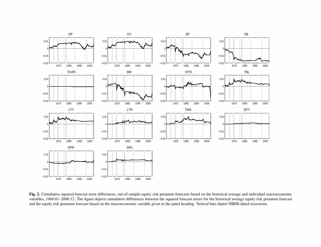
1975 1985 1995 2005−0.02
−0.01
0
0.01
DP
1975 1985 1995 2005−0.02
−0.01
0
0.01
DY
1975 1985 1995 2005−0.02
−0.01
0
0.01
EP
1975 1985 1995 2005−0.02
−0.01
0
0.01
DE
1975 1985 1995 2005−0.02
−0.01
0
0.01
SVAR
1975 1985 1995 2005−0.02
−0.01
0
0.01
BM
1975 1985 1995 2005−0.02
−0.01
0
0.01
NTIS
1975 1985 1995 2005−0.02
−0.01
0
0.01
TBL
1975 1985 1995 2005−0.02
−0.01
0
0.01
LTY
1975 1985 1995 2005−0.02
−0.01
0
0.01
LTR
1975 1985 1995 2005−0.02
−0.01
0
0.01
TMS
1975 1985 1995 2005−0.02
−0.01
0
0.01
DFY
1975 1985 1995 2005−0.02
−0.01
0
0.01
DFR
1975 1985 1995 2005−0.02
−0.01
0
0.01
INFL
Fig. 2. Cumulative squared forecast error differences, out-of-sample equity risk premium forecasts based on the historical average and individual macroeconomicvariables, 1966:01–2008:12. The figure depicts cumulative differences between the squared forecast errors for the historical average equity risk premium forecastand the equity risk premium forecast based on the macroeconomic variable given in the panel heading. Vertical bars depict NBER-dated recessions.

1975 1985 1995 2005
0
0.25
0.5
0.75
1
1.25
MA(1,9)
1975 1985 1995 2005
0
0.25
0.5
0.75
1
1.25
MA(1,12)
1975 1985 1995 2005
0
0.25
0.5
0.75
1
1.25
MA(2,9)
1975 1985 1995 2005
0
0.25
0.5
0.75
1
1.25
MA(2,12)
1975 1985 1995 2005
0
0.25
0.5
0.75
1
1.25
MA(3,9)
1975 1985 1995 2005
0
0.25
0.5
0.75
1
1.25
MA(3,12)
1975 1985 1995 2005
0
0.25
0.5
0.75
1
1.25
MOM(9)
1975 1985 1995 2005
0
0.25
0.5
0.75
1
1.25
MOM(12)
1975 1985 1995 2005
0
0.25
0.5
0.75
1
1.25
VOL(1,9)
1975 1985 1995 2005
0
0.25
0.5
0.75
1
1.25
VOL(1,12)
1975 1985 1995 2005
0
0.25
0.5
0.75
1
1.25
VOL(2,9)
1975 1985 1995 2005
0
0.25
0.5
0.75
1
1.25
VOL(2,12)
1975 1985 1995 2005
0
0.25
0.5
0.75
1
1.25
VOL(3,9)
1975 1985 1995 2005
0
0.25
0.5
0.75
1
1.25
VOL(3,12)
Fig. 3. Out-of-sample equity risk premium forecasts based on individual technical indicators, 1966:01–2008:12. Black (gray) lines delineate equity risk premiumforecasts in percent based on the technical indicator given in the panel heading (historical average). Vertical bars depict NBER-dated recessions.

1975 1985 1995 2005−0.01
−0.005
0
0.005
0.01
MA(1,9)
1975 1985 1995 2005−0.01
−0.005
0
0.005
0.01
MA(1,12)
1975 1985 1995 2005−0.01
−0.005
0
0.005
0.01
MA(2,9)
1975 1985 1995 2005−0.01
−0.005
0
0.005
0.01
MA(2,12)
1975 1985 1995 2005−0.01
−0.005
0
0.005
0.01
MA(3,9)
1975 1985 1995 2005−0.01
−0.005
0
0.005
0.01
MA(3,12)
1975 1985 1995 2005−0.01
−0.005
0
0.005
0.01
MOM(9)
1975 1985 1995 2005−0.01
−0.005
0
0.005
0.01
MOM(12)
1975 1985 1995 2005−0.01
−0.005
0
0.005
0.01
VOL(1,9)
1975 1985 1995 2005−0.01
−0.005
0
0.005
0.01
VOL(1,12)
1975 1985 1995 2005−0.01
−0.005
0
0.005
0.01
VOL(2,9)
1975 1985 1995 2005−0.01
−0.005
0
0.005
0.01
VOL(2,12)
1975 1985 1995 2005−0.01
−0.005
0
0.005
0.01
VOL(3,9)
1975 1985 1995 2005−0.01
−0.005
0
0.005
0.01
VOL(3,12)
Fig. 4. Cumulative squared forecast error differences, out-of-sample equity risk premium forecasts based on the historical average and individual technicalindicators, 1966:01–2008:12. The figure depicts cumulative differences between the squared forecast errors for the historical average equity risk premium forecastand the equity risk premium forecast based on the technical indicator given in the panel heading. Vertical bars depict NBER-dated recessions.
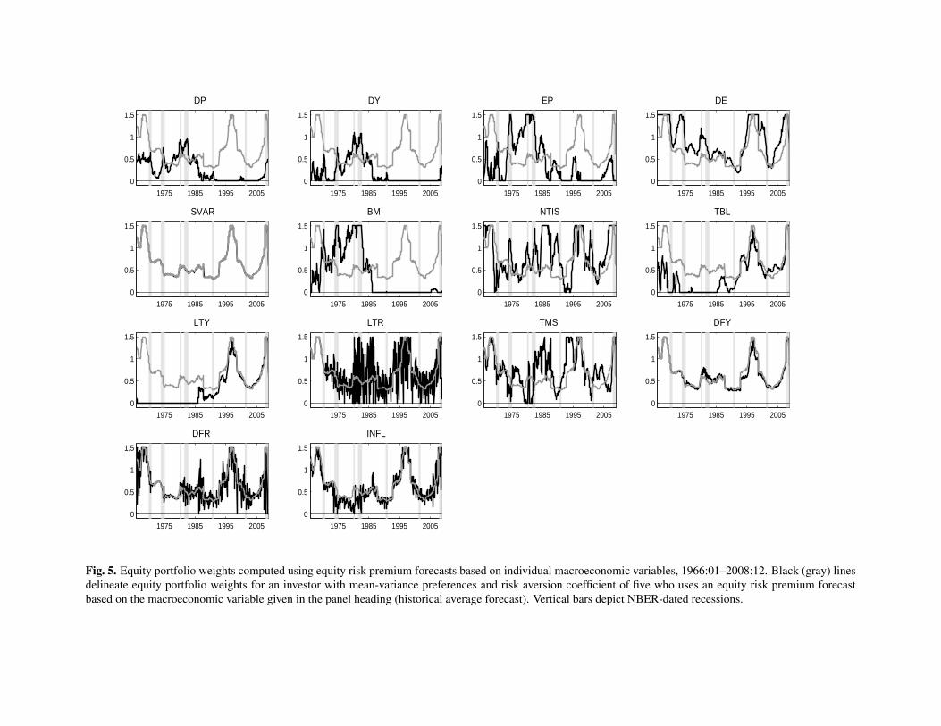
1975 1985 1995 2005
0
0.5
1
1.5
DP
1975 1985 1995 2005
0
0.5
1
1.5
DY
1975 1985 1995 2005
0
0.5
1
1.5
EP
1975 1985 1995 2005
0
0.5
1
1.5
DE
1975 1985 1995 2005
0
0.5
1
1.5
SVAR
1975 1985 1995 2005
0
0.5
1
1.5
BM
1975 1985 1995 2005
0
0.5
1
1.5
NTIS
1975 1985 1995 2005
0
0.5
1
1.5
TBL
1975 1985 1995 2005
0
0.5
1
1.5
LTY
1975 1985 1995 2005
0
0.5
1
1.5
LTR
1975 1985 1995 2005
0
0.5
1
1.5
TMS
1975 1985 1995 2005
0
0.5
1
1.5
DFY
1975 1985 1995 2005
0
0.5
1
1.5
DFR
1975 1985 1995 2005
0
0.5
1
1.5
INFL
Fig. 5. Equity portfolio weights computed using equity risk premium forecasts based on individual macroeconomic variables, 1966:01–2008:12. Black (gray) linesdelineate equity portfolio weights for an investor with mean-variance preferences and risk aversion coefficient of five who uses an equity risk premium forecastbased on the macroeconomic variable given in the panel heading (historical average forecast). Vertical bars depict NBER-dated recessions.

1975 1985 1995 2005
0
0.5
1
1.5
MA(1,9)
1975 1985 1995 2005
0
0.5
1
1.5
MA(1,12)
1975 1985 1995 2005
0
0.5
1
1.5
MA(2,9)
1975 1985 1995 2005
0
0.5
1
1.5
MA(2,12)
1975 1985 1995 2005
0
0.5
1
1.5
MA(3,9)
1975 1985 1995 2005
0
0.5
1
1.5
MA(3,12)
1975 1985 1995 2005
0
0.5
1
1.5
MOM(9)
1975 1985 1995 2005
0
0.5
1
1.5
MOM(12)
1975 1985 1995 2005
0
0.5
1
1.5
VOL(1,9)
1975 1985 1995 2005
0
0.5
1
1.5
VOL(1,12)
1975 1985 1995 2005
0
0.5
1
1.5
VOL(2,9)
1975 1985 1995 2005
0
0.5
1
1.5
VOL(2,12)
1975 1985 1995 2005
0
0.5
1
1.5
VOL(3,9)
1975 1985 1995 2005
0
0.5
1
1.5
VOL(3,12)
Fig. 6. Equity portfolio weights computed using equity risk premium forecasts based on individual technical indicators, 1966:01–2008:12. Black (gray) linesdelineate equity portfolio weights for an investor with mean-variance preferences and risk aversion coefficient of five who uses an equity risk premium forecastbased on the technical indicator given in the panel heading (historical average forecast). Vertical bars depict NBER-dated recessions.

−2 −1 0 1 2 3 4
−6
−3
0
3
6Actual
−2 −1 0 1 2 3 4
−0.6
−0.3
0
0.3
0.6
DP
−2 −1 0 1 2 3 4
−0.6
−0.3
0
0.3
0.6
DY
−2 −1 0 1 2 3 4
−0.6
−0.3
0
0.3
0.6
EP
−2 −1 0 1 2 3 4
−0.6
−0.3
0
0.3
0.6
DE
−2 −1 0 1 2 3 4
−0.6
−0.3
0
0.3
0.6
SVAR
−2 −1 0 1 2 3 4
−0.6
−0.3
0
0.3
0.6
BM
−2 −1 0 1 2 3 4
−0.6
−0.3
0
0.3
0.6
NTIS
−2 −1 0 1 2 3 4
−0.6
−0.3
0
0.3
0.6
TBL
−2 −1 0 1 2 3 4
−0.6
−0.3
0
0.3
0.6
LTY
−2 −1 0 1 2 3 4
−0.6
−0.3
0
0.3
0.6
LTR
−2 −1 0 1 2 3 4
−0.6
−0.3
0
0.3
0.6
TMS
−2 −1 0 1 2 3 4
−0.6
−0.3
0
0.3
0.6
DFY
−2 −1 0 1 2 3 4
−0.6
−0.3
0
0.3
0.6
DFR
−2 −1 0 1 2 3 4
−0.6
−0.3
0
0.3
0.6
INFL
Fig. 7. Actual equity risk premium and equity risk premium forecasts based on individual macroeconomic variables near a U.S. business-cycle peak. The panelsshow the incremental change in the average difference between the actual equity risk premium or equity risk premium forecast based on the macroeconomic variablegiven in the panel heading and the historical average equity risk premium forecast two months before through four months after an NBER-dated peak. Actual andforecast values are measured in percent. Circles indicate point estimates and shaded areas depict 90% confidence bands.

−2 −1 0 1 2 3 4
−6
−3
0
3
6Actual
−2 −1 0 1 2 3 4−0.9
−0.6
−0.3
0
0.3MA(1,9)
−2 −1 0 1 2 3 4−0.9
−0.6
−0.3
0
0.3MA(1,12)
−2 −1 0 1 2 3 4−0.9
−0.6
−0.3
0
0.3MA(2,9)
−2 −1 0 1 2 3 4−0.9
−0.6
−0.3
0
0.3MA(2,12)
−2 −1 0 1 2 3 4−0.9
−0.6
−0.3
0
0.3MA(3,9)
−2 −1 0 1 2 3 4−0.9
−0.6
−0.3
0
0.3MA(3,12)
−2 −1 0 1 2 3 4−0.9
−0.6
−0.3
0
0.3MOM(9)
−2 −1 0 1 2 3 4−0.9
−0.6
−0.3
0
0.3MOM(12)
−2 −1 0 1 2 3 4−0.9
−0.6
−0.3
0
0.3VOL(1,9)
−2 −1 0 1 2 3 4−0.9
−0.6
−0.3
0
0.3VOL(1,12)
−2 −1 0 1 2 3 4−0.9
−0.6
−0.3
0
0.3VOL(2,9)
−2 −1 0 1 2 3 4−0.9
−0.6
−0.3
0
0.3VOL(2,12)
−2 −1 0 1 2 3 4−0.9
−0.6
−0.3
0
0.3VOL(3,9)
−2 −1 0 1 2 3 4−0.9
−0.6
−0.3
0
0.3VOL(3,12)
Fig. 8. Actual equity risk premium and equity risk premium forecasts based on individual technical indicators near a U.S. business-cycle peak. The panels showthe incremental change in the average difference between the actual equity risk premium or equity risk premium forecast based on the technical indicator given inthe panel heading and the historical average equity risk premium forecast two months before through four months after an NBER-dated peak. Actual and forecastvalues are measured in percent. Circles indicate point estimates and shaded areas depict 90% confidence bands.

−4 −3 −2 −1 0 1 2−4
0
4
8Actual
−4 −3 −2 −1 0 1 2
−0.4
0
0.4
0.8
DP
−4 −3 −2 −1 0 1 2
−0.4
0
0.4
0.8
DY
−4 −3 −2 −1 0 1 2
−0.4
0
0.4
0.8
EP
−4 −3 −2 −1 0 1 2
−0.4
0
0.4
0.8
DE
−4 −3 −2 −1 0 1 2
−0.4
0
0.4
0.8
SVAR
−4 −3 −2 −1 0 1 2
−0.4
0
0.4
0.8
BM
−4 −3 −2 −1 0 1 2
−0.4
0
0.4
0.8
NTIS
−4 −3 −2 −1 0 1 2
−0.4
0
0.4
0.8
TBL
−4 −3 −2 −1 0 1 2
−0.4
0
0.4
0.8
LTY
−4 −3 −2 −1 0 1 2
−0.4
0
0.4
0.8
LTR
−4 −3 −2 −1 0 1 2
−0.4
0
0.4
0.8
TMS
−4 −3 −2 −1 0 1 2
−0.4
0
0.4
0.8
DFY
−4 −3 −2 −1 0 1 2
−0.4
0
0.4
0.8
DFR
−4 −3 −2 −1 0 1 2
−0.4
0
0.4
0.8
INFL
Fig. 9. Actual equity risk premium and equity risk premium forecasts based on individual macroeconomic variables near a U.S. business-cycle trough. The panelsshow the incremental change in the average difference between the actual equity risk premium or equity risk premium forecast based on the macroeconomicvariable given in the panel heading and the historical average equity risk premium forecast four months before through two months after an NBER-dated trough.All forecasts are measured in percent. Circles indicate point estimates and shaded areas depict 90% confidence bands.

−4 −3 −2 −1 0 1 2−4
0
4
8Actual
−4 −3 −2 −1 0 1 2
−0.6
−0.3
0
0.3
0.6MA(1,9)
−4 −3 −2 −1 0 1 2
−0.6
−0.3
0
0.3
0.6MA(1,12)
−4 −3 −2 −1 0 1 2
−0.6
−0.3
0
0.3
0.6MA(2,9)
−4 −3 −2 −1 0 1 2
−0.6
−0.3
0
0.3
0.6MA(2,12)
−4 −3 −2 −1 0 1 2
−0.6
−0.3
0
0.3
0.6MA(3,9)
−4 −3 −2 −1 0 1 2
−0.6
−0.3
0
0.3
0.6MA(3,12)
−4 −3 −2 −1 0 1 2
−0.6
−0.3
0
0.3
0.6MOM(9)
−4 −3 −2 −1 0 1 2
−0.6
−0.3
0
0.3
0.6MOM(12)
−4 −3 −2 −1 0 1 2
−0.6
−0.3
0
0.3
0.6VOL(1,9)
−4 −3 −2 −1 0 1 2
−0.6
−0.3
0
0.3
0.6VOL(1,12)
−4 −3 −2 −1 0 1 2
−0.6
−0.3
0
0.3
0.6VOL(2,9)
−4 −3 −2 −1 0 1 2
−0.6
−0.3
0
0.3
0.6VOL(2,12)
−4 −3 −2 −1 0 1 2
−0.6
−0.3
0
0.3
0.6VOL(3,9)
−4 −3 −2 −1 0 1 2
−0.6
−0.3
0
0.3
0.6VOL(3,12)
Fig. 10. Actual equity risk premium and equity risk premium forecasts based on individual technical indicators near a U.S. business-cycle trough. The panels showthe incremental change in the average difference between the actual equity risk premium or equity risk premium forecast based on the technical indicator given inthe panel heading and the historical average equity risk premium forecast four months before through two months after an NBER-dated trough. All forecasts aremeasured in percent. Circles indicate point estimates and shaded areas depict 90% confidence bands.

1970 1975 1980 1985 1990 1995 2000 2005
0
0.5
1
1.5
PC forecasts (%)
1970 1975 1980 1985 1990 1995 2000 2005
−0.01
0
0.01
0.02
Difference in cumulative SFE, HA/PC
1970 1975 1980 1985 1990 1995 2000 2005
0
0.5
1
1.5
PC equity weights
Fig. 11. Out-of-sample equity risk premium forecasts based on macroeconomic variables and technical indicators taken together, 1966:01–2008:12. Black (gray)line in the top panel delineates the principal component (historical average) equity risk premium forecast. The principal component (PC) equity risk premiumforecast is based on the first k principal components of the 14 macroeconomic variables and 14 technical indicators taken together, where k is selected using theOnatski (2009) ED algorithm. The middle panel depicts cumulative differences between the squared forecast errors for the historical average and PC equity riskpremium forecasts. Black (gray) line in the bottom panel delineates the equity portfolio weight for an investor with mean-variance preferences and risk aversioncoefficient of five who uses the PC equity risk premium forecast (historical average forecast). Vertical bars depict NBER-dated recessions.