Forecasting Method for General Aviation Aircraft and Their

50

commuter passenger traffic at Logan increased by 40 percent between 1977 and 1978.

Such volatility in the presence of not previously experienced changes is, of course, difficult to forecast, and many projections made in the mid-1970s dramatically underestimated growth of commuter traffic. However, aside from this type of unforeseeable effect, many earlier (i.e., late 1960s) forecasts systematically overpredicted future activity. Although this paper does not detail an explanation of these inaccuracies, the analysis undertaken in this study isolated two principal causes. First, economic growth was projected to be much higher than the actual experience of the 1970s. Second, early forecasting models had income elasticities that are now believed to be too high and air-fare elasticities that are believed to be too low.

Another finding during the course of the study has been the limited amount of consistent and reliable data available for site-specific forecasts. Differences in the categorization of activity between data sources and between available and desired data items often constrain modeling efforts. For example, the adequacy of average yield as an explanatory variable in demand-forecasting equations during years when the rate schedule is complex and demand oriented was subject to some doubt. Although we found that average yield provides an adequate measure of fare levels and find no evidence of large backcasting residuals when it is used, the unavailability or the known inaccuracies and biases of data that measure both activity levels and causal factors often make informed judgment an appropriate forecasting tool.

ACKNOWLEDGMENT

The forecasting project reported here was funded by the Massachusetts Port Authority under a planning

Transportation Research Record 768

grant from the Federal Aviation Administration. We would like to acknowledge the assistance provided by Mitchell Kellman and Cynthia Kagno of Charles River Associates. The opinions and conclusions expressed or implied in the paper are ours and are not necessarily those of the Transportation Research Board, the National Academy of Sciences, or the Massachusetts Port Authority.

REFERENCES

1 . Charles River Associates, Inc. Logan International Airport Passenger and Air Cargo Forecasts. Massachusetts Port Authority, Dec. 1979.

2. P.K. Verleger, Jr. Models of the Demand for Air Transportation. Bell Journal of Economics and Management Science, Vol. 3, 1972, pp. 412-457.

3 . 1975 Statistical Abstract of the United States. Bureau of the Census, U.S. Department of Commerce, 1975.

4. R.W. Gilmer. Services and Energy in U.S. Economic Growth. U.S. Department of Energy, Inotitute for Energy Analysis, Oak Ridge, TN, 1977.

5. Charles River Associates, Inc. Review and Evaluation of Selected Large-Scale Energy Models. Electric Power Research Institute, Cambridge, MA, 1977.

6. G. Deosaran, H. Sweezy, and R. Van Duzee. Forecasts of Commuter Airlines Activity, Appendix C. Federal Aviation Administration, U.S. Department of Transportation, Rept. FAA-AVR-77-28, 1977.

7. J. Rocks and H. Zabronsky. Study and Forecast of General Aviation Operations at 60 Medium-Hub Airports. Federal Aviation Administration, u.s. Department of Transportation, Rept. DOT-FAA-77WAI-726, 1978.

Publication of this paper sponsored by Committee on Aviation Demand Forecasting.

Forecasting Method for General Aviation Aircraft and Their Activity BRUCE C. CLARK AND JAMES R. TANKERSLEY

This paper describes the formulation and application of a general aviation (GA) forecasting model within the context of the North Central Texas regional airport system planning process. The objective of the model was to provide a means of forecasting registered county-level GA aircraft ownership and the activity of those aircraft (hours flown) that allows public policymakers and planners to assess the impact of policy and economic growth alternatives on GA demand. The bottom-to-top econometric and time-series model developed through this effort achieved these objectives with statistical results that varied across the 19 counties and four aircraft types. Finally, a feature of this model uncom.mon to other GA forecasting models is that the demand for aircraft is specified to be (among other things) a function of the demand for air travel (hours flown).

The North Central Texas Airport System Plan, adopted by the Regional Transportation Policy Advisory Committee (RTPAC) on November 16, 1974, presented the findings of a comprehensive two-year analysis of existing and future activity in the 19-county area defined by the North Central Texas and Texoma state

planning regions. The plan identified existing airport facilities, forecast aviation demand through the year 1990, and recommended the staged development of a system of public airports (to include improvements to both proposed and existing airports) to meet that demand.

With the adoption of the plan, efforts of the RTPAC staff focused on assisting local governments in plan implementation. In addition, efforts were made to update the plan in response to changing conditions within the aviation community and within local communities. An outgrowth of these efforts was a realization that the technical planning process underlying the system plan did not allow for a rapid, comprehensive response to technical or policy issues that were raised by elected officials, airport managers, and the general public.

For example, a major issue raised by groups opposed to new airports was whether there was a need


to build new general aviation (GA) airports if fuel prices continued their rapid climb: The assumption was that rapid fuel price increases were equated to an equally rapid decline in GA activity. Another issue was what effect either delaying the construction of or not building a recommended airport would have on existing facilities. In each case, neither the plan nor the technical planning process provided a mechanism for developing an analytically based response to the issue raised.

The identified weaknesses in the existing plan and planning process led to the development of a definition for a new technical GA airport system planning process for the North Central Texas region. This paper presents one component of that process: a forecasting method for GA aircraft and their activity. A necessary feature of any aviation forecast is the identification and measurement of the factors that affect aviation growth. The indicators of regional GA growth in this forecasting method are the number of aircraft (by type of aircraft) registered with the Federal Aviation Administration (FAA) and the hours flown by those aircraft. The model is based on the hypothesis that regional growth is, in general, a function of fuel costs, income, and general credit conditions. As with most forecasting models, data limitations prevent the method presented here from being a complete representation of all factors that affect GA growth.

The ultimate goal of a regional aviation forecasting effort is the generation of airport-specific activity forecasts. Therefore, a bottom-to-top approach to forecasting was assumed in the model's construction; i.e., the smallest geographic area was used for which sufficient data were available to support the forecasting effort. This was each of the 19 individual counties. When data limitations made direct estimates of county-level activity impossible, county-level estimates were derived as marginal products of regional estimates.

The forecasting model presented here does not provide future estimates of local and itinerant operations, which are variables of interest to federal, state, and local planners. There is a threefold reason for not forecasting aircraft operations directly. First, accurate historical operational data at the level of specificity required are simply not available. Second, the costs associated with initiating such a data collection effort are beyond the financial resources of a regional airport system planning effort. A third and more fundamental reason for not forecasting operations directly is that, in the perception of the aircraft owner, the total hours the aircraft has been flown represents the amount of available aircraft service that has been consumed over the lifetime of the aircraft.

It can therefore be argued that the theoretical measure of GA activity is total hours flown. Airport operations represent a complementary benefit in the consumption of GA hours flown and need not (and perhaps should not) be forecast directly. Since we recognized that (theory aside) we still needed forecasts of airport operations for planning purposes, data by which forecasts of total hours flown could be converted to aircraft operations were derived from a survey of registered aircraft owners in the region performed by the North Central Texas Council of Governments (NCTCOG). Further, NCTCOG is developing a GA demand and assignment model that will allow county-level aviation forecasts to be assigned to specific airports. This will enable planners to assess future needs at individual airports.

51

FORECASTING METHODS AVAILABLE

There are three established long-term forecasting methods employed in GA forecasting at the regional level: (a) the regional-share method, (b) the time-series (trend) method, and (c) the econometric method. It is common practice to use all three methods in a forecast to evaluate the best method or combination of methods. This formal exercise has resulted in some general agreement about the effectiveness of each method or combination of methods by aviation planners. More specifically, the consensus favors a combination of methods (b) and (c) while regarding method (a) as more or less a descriptive statistic.

The regional-share forecast is performed by observing alternative national forecasts from which one can compute the future alternative regional forecasts by calculating the region's percentage share of the national total and extending the series into the future. The implication of a constant market structure is the flaw that aviation planners reject (ll· Regional share is really the outcome of regional aviation growth. Consequently, the results of regional GA forecasts are often illustrated by computing the regional share only for purposes of comparison.

A popular forecasting method among aviation planners today is the time-series (trend) method. In this method, the variable of interest is expressed as a function of time or as a function of its own variation over time. These models take on a wide variety of functional forms and incorporate different estimation methods. They can generally be classified as deterministic or stochastic (~l. The Box-Jenkins models developed by FAA to forecast quarterly itinerant and local operations are examples of s .tochastic models <ll. In general, deterministic and stochastic time-series models do not predict w.ell in the long run because of their intrinsic naturei i.e., the forecast variable is not related to any causal variable over time. For this reason, their use is generally confined to short-term forecasts.

The econometric method is most often used to make long-term forecasts. Econometric models attempt to simulate economic behavior in the real world based on well-established relationships with other variables over time. An econometric model may consist of one or more equations, and each equation may consist of one or more variables. These models are typically constructed to explain the movement in one or more key variables (endogenous variables) by the movement in other outside variables (exogenous variables). By altering the values of the exogenous variables in the model, the forecaster can simulate real-world events based on alternative assumptions about the future. The examination of alternative long-term trends is a useful planning exercise for establishing confidence limits in the uncertain future.

The forecasting model constructed for GA activity combines both the econometric and the time-series methods in its structure. In this hybrid approach, the error terms in the econometric model are used to construct a time-series model, which in turn is used to adjust the original econometric model for any temporal systematic bias in the original data (!l. The resulting transformed model is then used for forecasting.

DATA SOURCES

The FAA aircraft registration master file provided data on the number of aircraft and reported hours flown by aircraft type and county. In addition,

52

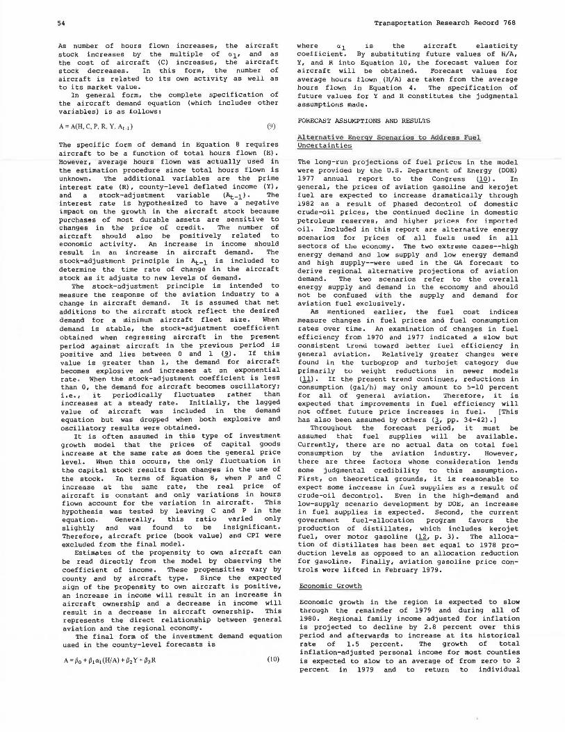
Figure 1. Economic model structure for , estimating GA activity. FUEL COST INDEX 1-----

BY TYPE

TRANSPORTATION COMFOOENT CONSUMER !>RICE INDEX

DEFLATED INCOME PER HOUSEHOLD 1-----"""'

REGICl'IAL AVERAC..£ HOURS FLOWN BY TYPE


REPORTED HOURS FLOWN BY TYPE/ BY COUNTY

REPORTING AIRCRAFT BY TYPE I BY COUNTY

AIRCRAFT ELASTICITY COEFFICIENTS BY TYPE/ BY COUNTY

MARGINAL HOURS FLOWN BY TYPE I BY COUNTY

information from the file on the make, model, and year of manufacture of the regional aircraft fleet was used to identify fuel-consumption rates of a sample of GA aircraft to construct a fuel cost index. Data on these variables were available for December 31, 1970, to December 31, 1977.

Other data sources included all the items and the transportation component of the consumer price index (CPI) from the Bureau of Labor Statistics for 1970-1977. The Aircraft Blue Book was also used to obtain fuel-consumption rates (gal/h). County and regional income data were taken from Sales and Marketing Management magazine's annual survey of buyer income. Finally, the prime rate of interest charged by banks was obtained from the 1978 economic report of the President.

THE MODEL

An illustration of the structural relationships in the GA forecasting model is presented in Figure 1. This structure assumes that activity is determined by general regional economic conditions and those economic factors particular to aviation. First a production relationship is established between reported hours flown and the number of aircraft units that report hours flown in each county. Aircraft elastic! ty coefficients are obtained from these estimates, which are used to calibrate regional average hours flown at the county level. Regional average hours flown for each aircraft type is determined by a fuel cost index, the transportation CPI, and deflated household income. The calibrated average hours flown estimates (marginal productivities) are used with deflated county income and national prime-interest-rate data to forecast the number of aircraft by aircraft type in each county. Finally, the calibrated estimates of average hours flown are applied to the aircraft forecasts to obtain total hours flown.

Production Function

The production function is specified in nonlinear form as follows:

RH=a0 RA"l (!)

where

liOURS FLOWN BY TYPE/BY COONTY

PRIME INTEflEST i---RATE

AIRCRAFT BY TYPE BY COUNTY

DEFLATED PERSONAL INCOME BY COUNTY

RH = reported hours flown, RA = aircraft that report hours flown, and

ao and a 1= constants.

The parameter a 1 is interpreted as the long-term aircraft input elasticity coefficient. In general, input elasticity of any factor of production measures the percentage response of output from a percentage change in the factor of production. Thus, aircraft elasticity provides a measure of the sensitivity of hours flown from a change in the regional aircraft fleet size. To perform regression analyses, Equation 1 is linearized by logarithmic transformation into

Jn RH = Ina0 + a1 InRA (2)

If we assume that Equation 2 represents the true relationship between total hours flown and total aircraft, Equation 1 can be rewritten as follows:

(3)

where H represents total hours flown and A represents total aircraft.

According to general-production theory, labor and other resources as well as capital a:re included in the production function. These constitute the variable production inputs in the short term when the capital stock is assumed constant. In this case, labor (pilots) and other resources (fuel) are not known. The omission of these variables from the equation may result in biased estimates of aircraft elastici tyi i.e., the normal probability distribution of a1 may not have as its mean value the true population value of a 1 • However, the effect of the specification bias must be weighed against the following:

l. The magnitude of any possible bias that results from omission of unknown.

specification variables is

2. Any unknown bias that results from omission of variables implies the presence of multicolinearity in the regression coefficients and results in biased least-squares parameter estimates if the variable is included (5).

3. The objective in for-;casting is to obtain estimates of minimum-variance parameters and not necessarily unbiased estimates of parameters.


In practice, it is the extent of the bias that is most important in model specification. If a high correlation exists between aircraft and pilots, the coefficient u1 will be biased whether or not pilots are included in the equation. With reference to statement 3, a biased regression coefficient that results from an omitted variable has been proved to be more efficient (has smaller variance) than the regression-coefficient estimate when the omitted variable is included in the equation (~). For forecasting purposes, minimum-variance estimators are typically chosen over all other estimators in small samples because they are more precise than an unbiased estimator with high variance.

Another factor that potentially affects the elasticity coefficients is the type of use to which the region's aircraft fleet is applied.

In the course of model development, aircraft use was carefully examined and ultimately rejected by NCTCOG staff in the specification of the production function. County cross-tabulations of hours flown by primary use yielded sample sizes in many counties that were too small for accurate modeling and prediction. In addition, most aircraft types were found to be dominated by one or two primary uses; e.g., air-taxi and executive uses are predominant for jet aircraft and personal and instructional uses are predominant for single-engine piston-powered aircraft (.§_, p. 10). This suggests that, for a given aircraft typer changes in use are minimal over time. Differences in equipment, pilot-licensing requirements, and aircraft performance may present limitations to an aircraft's use. Therefore, it was assumed that changes in primary use for each aircraft type would not be significant during the forecast period.

Demand Equation for Ave r age Hours Flown

average hours flown has both price and income

Specifically, its

The equation for regional been specified to include effects on GA activity. functional form appears as

H/ A = ~o - ~ 1 Fl/TCPI + ~2 INC/HH

where

H reported hours flown in the region, A = airqraft that report,

FI = regional fuel cost index,

(4)

TCP! ~ regional transportation component of the CPI,

INC regional income deflated by CPI for all goods, and

HH number of households in the region.

The ratio FI/TCP! represents the real cost of aircraft operation ahd thus its expected sign is negative. Since GA operating costs are not included in TCP!, the ratio is a good measure of the relative impact of changes in aviation variable costs to other transportation costs. When FI increases relative to TCP!, average hours flown decreases, and when TCP! increases relative to FI, average hours flown increases. Thus, a substitutional relationship is hypothesized between general aviation and other modes of transportation. The expected sign of INC/HH is positive. The hypothesis here is that as income per unit (household) increases, average hours flown increases.

Average hours flown is used as the measure of GA activity demand only because total hours flown is not known. Treating reported hours flown as a sample drawn from the regional population of aircraft owners, the appropriate measure of demand

53

is the average or mean value of the sample. The assumption involved here is that the sample average is equal to the population average for the region. At the county level, approximately 50-60 percent of aircraft owners reported hours flown, but the sample sizes at the county level for the less-populated counties are very small. Therefore, average hours flown is estimated at the regional level in order to use a larger sample size.

To measure the variable cost impact on the demand for hours flown, a regional fuel cost index was constructed for the period 1970-1977. The construction of this index served two purposes: (a) to convert the cost per gallon of fuel into a measure of the cost per hour of flying over time and (b) to account for changes in fuel consumption rates per flight hour due to variations in the number of aircraft types over time. Specifically, the Ratchford Cl) index was used for this purpose, and it appears as follows:

(5)

where

FI fuel cost index, ci fuel consumption rate (gal/h) for the ith

aircraft make and model, G regional price per gallon of aviation

gasoline or kerojet fuel, Hi hours flown by the ith aircraft make and

model, and t time.

D~mand Equation for Aircra.ft Investment

Unlike other regression models used to forecast the GA fleet, the aircraft demand equation included in this model specifies GA aircraft to be (among other things) a function of GA activity (,!!). In this context, the demand for aircraft can be considered as a derived demand for air travel. In other words, the desired stock of aircraft does not reflect the demand for aircraft per se but a demand for the flow of services that aircraft can provide over time, i.e., hours flown.

The theory employed in the aircraft investment equation is a variant of the general flexible accelerator model developed by Jorgenson and Siebert C.~l • In this model, a variable relationship is derived from the production function, which relates the increase in hours flown to the level of the regional aircraft stock. First, it is assumed that the aircraft stock will expand until the marginal product of aircraft equals the real user cost of aircraft. In the competitive case, the real marginal user cost of adding one more aircraft to the regional aviation fleet is equal to the market price of aircraft. The marginal product of aircraft derived from the production function is as follows:

(6)

Then, in user equilibrium, real marginal user cost is equal to marginal product:

0:1 (H/ A) = (C/P) (7)

where C is the price of aircraft and P is the CPI. When we solve for A in Equation 7, the equilibrium capital stock is as follows:

A=a:1PH/C (8)

54

As number of hours flown increases, the aircraft stock increases by the multiple of 01, and as the cost of aircraft (Cl increases, the aircraft stock decreases. In this form, the number of aircraft is related to 1 ts own activity as well as to its market value.

In general form, the complete specification of the aircraft demand equation (which includes other variables) is as follows:

A= A(H, C, P, R, Y, At_1) (9)

The specific form of demand in Equation 8 requires aircraft to be a function of total hours flown (H). However, average hours flown was actually used in the estimation procedure since total hours flown is unknown. The additional variables are the prime interest rate (R), county-level deflated income (Y), and a stock-adjustment variable <At-1>· The interest rate is hypothesized to have a negative impact on the growth in the aircraft stock because purchases of most durable assets are sensitive to changes in the price of credit. The number of aircraft should also be positively related to economic activity. An increase in income should result in an increase in aircraft demand. The stock-adjustment principle in At-1 is included to determine the time rate of change in the aircraft stock as it adjusts to new levels of demand.

The stock-adjustment principle is intended to measure the response of the aviation industry to a change in aircraft demand. It is assumed that net additions to the aircraft stock reflect the desired demand for a minimum aircraft fleet size. When demand is stable, the stock-adjustment coefficient obtained when regressing aircraft in the present period against aircraft in the previous period is positive and lies between 0 and 1 <.~.>. If this value is greater than 1 1 the demand for aircraft becomes explosive and increases at an exponential rate . When the stock-adjustment coefficient is less than O, the demand for aircraft becomes oscillatory; i.e., it periodically fluctuates rather than increases at a steady rate. Initially, the lagged value of aircraft was included in the demand equation but was dropped when both explosive and oscillatory results were obtained.

It is often assumed in this type of investment growth model that the prices of capital goods increase at the same rate as does the general price level. When this occurs, the only fluctuation in the capital stock results from changes in the use of the stock. In terms of Equation 8, when P and C increase at the same rate, the real price of aircraft is constant and only variations in hours flown account for the var i at i on i n aircraft. This hypothesis was tested by leaving C and P in the equation. Generally, this ratio varied only slightly and was found to be insignificant. Therefore, aircraft price (book value) and CPI were excluded from the final model.

Estimates of the propensity to own aircraft can be read directly from the model by observing the coefficient of income. These propensities vary by county and by aircraft type. Since the expected sign of the propensity to own aircraft is positive, an increase in income will result in an increase in aircraft ownership and a decrease in income will result in a decrease in aircraft ownership. This represents the direct relationship between general aviation and the regional economy.

The final form of the investment demand equation used in the county-level forecasts is

(IO)


where a 1 is the aircraft elasticity coefficient. By substituting future values of H/A, Y, and R into Equation 10, the forecast values for aircraft will be obtained. Forecast values for average hours flown (H/A) are taken from the average hours flown in Equation 4. '.l'he specification of future values for Y and R constitutes the judgmental assumptions made.

FOliECAST ASSUMPTIONS AND RESULTS

Alternative Energy Scenarios to Address Fuel Uncertainties

The long-run projections of fuel prices in the model were provided by the U.S. Department of Energy (DOE) 1977 annual report to the Congress (10). In general, the prices of aviation gasoline an~kerojet fuel are expected to increase dramatically through 1982 as a result of phased decontrol of domestic crude-oil prices, the continued decline in domestic petroleum reserves, and higher pricf!s for imported oil. Included in this report are alternative energy scenarios for prices of all fuels used in all sectors of the economy. The two extreme cases--high energy demand and low supply and low energy demand and high supply--were used in the GA forecast to derive regional alternative projections of aviation demand. The two scenarios refer to the overall energy supply and demand in the economy and should not be confused with the supply and demand for aviation fuel exclusively.

As mentioned earlier, the fuel cost indices measure changes in fuel prices and fuel consumption rates over time. An examination of changes in fuel efficiency from 1970 and 1977 indicated a slow but consistent trend toward better fuel efficiency in general aviation. Relatively greater changes were found in the turboprop and turbojet category due primarily to weight reductions in newer models (11) . If the present trend continues, reductions in consumption (gal/h) may only amount to 5-10 percent for all of general aviation. Therefore, it is expected that improvements in fuel efficiency will not offset future price increases in fuel. [This has also been assumed by others (1, pp. 34-42) .]

Throughout the forecast period, it must be assumed that fuel supplies will be available. Currently, there are no actual data on total fuel consumption by the aviation industry. However, there are three factors whose consideration lends some judgmental credibility to this assumption. First, on theoretical grounds, it is reasonable to expect some increase in fuel supplies as a result of crude-oil decontrol. Even in the high-demand and low-supply scenario development by DOE, an increase in fuel supplies is expected. Second, the current government fuel-allocation program favors the production of distillates, which includes kerojet fuel, over motor gasoline (11_, p. 3). The allocation of distillates has been set equal to 1978 production levels as opposed to an allocation reduction for gasoline. Finally, aviation gasoline price controls were lifted in February 1979.

Economic Growth

Economic growth in the region is expected to slow through the remainder of 1979 and during all of 1980. Regional family income adjusted for inflation is projected to decline by 2.8 percent over this period and afterwards to increase at its historical rate of 1. 5 percent. The growth of total inflation-adjusted personal income for most counties is expected to slow to an average of from zero to 2 percent in 1979 and to return to individual


historical growth rates by 1981. The primary cause of the expected decline in economic growth is the anticipation of double-digit inflation through 1982. Inflation is expected to average 10.5 percent during the period 1979-1982, the primary cause being rising energy prices and previously built-up inflationary expectations.

Prime Interest Rate

It is assumed that the prime interest rate charged by banks will reach its peak in 1979 and the average for the year will be 11.25 percent. Any decline in the prime rate will be slow through 1982, primarily as a result of high inflation. The average for the 1980s should be about 8. 5 percent as compared with the average 7.9 percent during the 1970s. Results from the model indicate that interest rates had a slight dampening effect on regional aircraft investment.

Forecast Results

The model structure described provides county-level estimates of aircraft types. For the 19-county North Central Texas area, this provided 152 separate sets of forecast results. For the purposes of reporting the model results, the 19-county forecasts have been summed to reflect a regional forecast.

Figures 2-9 provide a graphic presentation of the forecasts for the North Central Texas and Texoma state planning regions. Although the curves exhibit an overall upward trend over the forecast period, each reflects the anticipated negative influences of rapid increases in fuel prices due to deregulation in the early 1980s coupled with continued high

Figure 2. Estimated number of single-engine piston aircraft.

5500

5000

4500

4000

= ~ 3500 (,,) .. c

3000

2500

2000

1970

1l ,~,, ,;,

,ii Low Energy Demand/ 1~1 High Supply ~

1;1 ,;,

1975

Year

l' ll l ,, ,' 1•,

,t/ ,#1 ,,,

,I/ ,~,'

High Energy Demand/ Low Supply

1980 1985 1990

55

inflation. For example, the total regional aircraft stock is expected to grow at an annual rate of 3.5-4.2 percent over the seven-year period from 1978 to 1984, compared with a 6. l percent annual growth rate from 1971 to 1977.

Most important, the distinguishing feature of

Figure 3. Estimated total hours flown by single-engine piston aircraft.

1400

1250

1100

950

800

650

500

1970

,. l I ,; .

,• ,' l , Low Energy Demand/ / /

High Supply ~ f' l #' I

1975

" I f' I ,, l #' I i I

#' I , 1 I

I I ,,,_,.J / -, I

' ,1. ' .. ' High Energy Demand/

Low Supply

1980 1985 1990

Year

Figure 4. Estimated number of multiengine pistpn aircraft.

900

800

700

= l? (,,) 600 ..

Ci

500

400

1970

,;j'. If,,'-' ;'1

Low Energy Demand/ {I High Supply 11o., I'/

1975

..,... "" ~,.,

~~/,.#

"'., l' JI I 1r/ ,,,,, "fie.

~., ....... High Energy Demand/

Low Supply

1980

Year

1985 1990

56

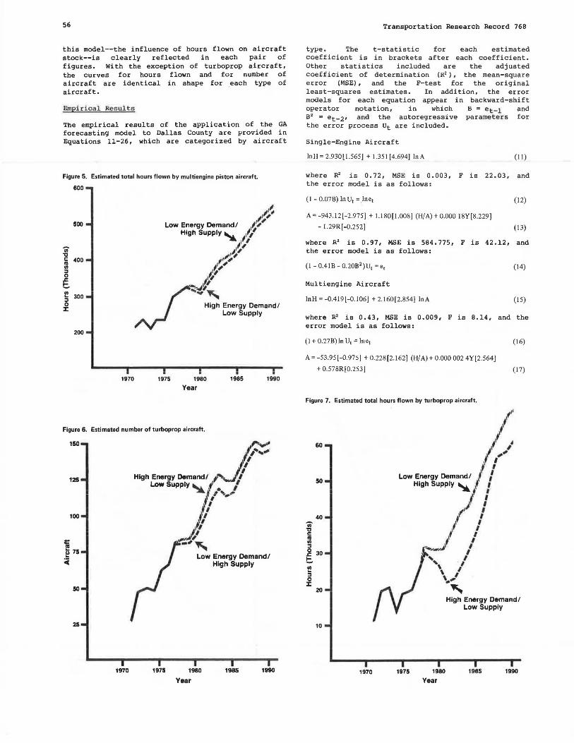
this model--the influence of hours flown on aircraft stock--is clearly reflected in each pair of figures. With the exception of turboprop aircraft, the curves for hours flown and for number of aircraft are identical in shape for each type of aircraft.

Empiri.cal Results

The empirical results of the application of the GA

forecasting model to Dallas County are provided in Equations 11-26, which are categorized by aircraft

Figure 5. Estimated total hours flown by multiengine piston aircraft.

600

500

iii 'ti i 400 Cll :I 0

E. ~ 300 0 :J:

200

1970

ll, I''

Low Energy Demand/ /'' High Supply~ ii/ ,1,

,~, ,,1, ;', l,'

i"'

J_,~.,

.--1), High Energy Demand/

Low Supply

1975 1980 Year

1985 1990

Figura 6. Estimated number of turboprop aircraft.

150

125

100

i ~ 75 ... c

so

15

1970

~ /, .... ,. ;~'

High Energy Demand/ ,,.,.._// Low Supply 111.... f • ,' ..,.., , ,_ ..

I' ll ,f/ ,,, l'

"=''' Low Energy Demand/

High Supply

1975 1980

Year 1985 1990


type. The t-statistic for each estimated coefficient is in brackets after each coefficient. Other statistics included are the adjusted coefficient of determination (R2 ), the mean-square error (MSE), and the F-test for the original least-squares estimates. In addition, the error models for each equation appear in backward-shift operator notation, in which B = et-1 and B2 = et-2• and the autoregressive parameters for the error process Ut are included.

Single-Engine Aircraft

lnH = 2.930[1.565) + 1.351 [4.694) lnA (11)

where R2 is O. 72, MSE is 0.003, F is 22.03, and the error model is as follows:

(1 - 0.07B) In U1 = ,lne1 (12)

A= -943.12(-2.975) + 1.180[1.008) (H/A) + 0.000 18Y[8.229)

- l.29R[-0.252] (13)

where R2 is 0.97, MSE is 584.775, F is 42.12, and the error model is as follows:

(14)

Multiengine Aircraft

lnH = -0.419(-0.106) + 2.160[2.854} lnA (15)


(1 + 0.27B)ln U1 = lne1 (16)

A= -53.95(-0.975) + 0.228(2.162) (H/A) + 0.000 002 4Y[2.564]

+ 0.578R[0.253] (17)

Figure 7. Estimated total hours flown by turboprop aircraft.

60

50

40 iii 'ti c ftl Cll :I 0 30 .c !:. Cll ... :I 0 :J:

20

10

1970

~,,

#' i

#' ~' ' 1' , l ,,

l I . ' Low Energy Demand/ l /

High Supply 111..., 1f I

1975

.._, I

t' I ~' I

;'" ' #' I I' I

#' I ,, ' -,,.-/J} l ,, '

\ I \ I ,_,,,

' High Energy Demand/

1980

Year

Low Supply

1985 1990



(18)

Turboprop Aircraft

lnH = 7.148[6.919] + 0.698[2.249] lnA (19)


(1+0.1 lB) lnU1 = lne 1 (20)

A= -105.06[-6.440) - 0.061 [-2.908) (H/A) + 0.0000!6Y[l1.477)

+ 0.845R[3.627) (21)


(22)

Turbojet Aircraft

lnH = 4.445[1.965) + 1.570[2.370] lnA (23)


(I - 0.25B) In U1 = lne1 (24)

A= -239.92[-5.222) + 0.129[4.137](H/A) + 0.000 025Y[6.155]

- 3.701R[-3.054] (25)


(26)

Figure 8. Estimated number of turbojet aircraft.

280

240

200

160

120

80

40

1970

l ~; I

" ' l ,, "' , i' I

Low Energy Demand/ 1f ,' High Supply ~ 1# I

l I ;' I ,, I ;' I

f' I #' I

1l / ,. 1'

, I \ ,

l ''•' It,' H;g~oo<gy Demoodl N Low Supply

1975 1980 19a5 1990

Year

57

Equations 27-34 give the results for regional average hours flown.

Single-Engine Aircraft

H/A = 211.761 [4.118) - 0.861 [-1.954) GF/TCPl

+ 0.0029[0.756) INC/HH (27)


Multiengine Aircraft

H/A = -59.852[-0.403] - 0.390[-0.283] GF/TCPl

+ 0.0203[1.552] INC/HH

(28)

(29)

where R2 is 0.26, MSE is 241. 74, F is 2.53, and the error model is as follows:

(30)

Turboprop Aircraft

H/A = 1244.01 [7.484) - 8.002(-4.771) KF/TCPl (31)

where R2 is 0.69, MSE is 859.70, Fis 22.76, and the error model is as follows:

(32)

Turbojet Aircraft

H/A = 1565.50[5.049) - 10.395(-3.344) KF/TCPI (33)


(34)

Figure 9. Estimated total hours flown by turbojet aircraft.

280

Iii 'C

240

200

~ 160 Cl) ::I 0

~ ~ 120 0 J:

80

40

,, l

•' i •'

•' •' •' ; t' I

i / Low Energy Demand/ f 1 High Supply " fl I

f I t1 I

1' I t' I l I

;' I i I

'""'""'' J l l ;t I ~- I "\/ \_,,~

High Energy Demand/ Low Supply

1970 1975 1980 1985 1990

Year

58

Table 1. Sensitivity analysis of dependent variables for selected years.

Percentage Change from Baseline Forecast Relative to a 1 % Increase in Fuel Cost Index

Depende11t Variable 1979 1981 1983 1985 1990

Aircraft Single-engine -0.09 -0.08 -0.07 -0.07 -0.08 Multienglne 0.00 0.00 0.00 0.00 0.00 Turboprop 0.00 0.00 0.00 0.00 0.00 Turbojet -1.94 -1.56 -1.27 -1.11 -0.78

Hours flown Single-engine -0.14 -0.30 -0.32 -0.47 -0.74 Multiengine -1.07 -0.13 -0.12 -0.11 -0.28 Turboprop -10.66 -9.47 -9.16 -9.98 -10.68 Turbojet -2.94 -6.81 -6.16 -5.12 -4.51

These equations indicate that the real cost of aviation fuel has a significant impact on average hours flown. However, the t-statistics for each equation are only asymptotically valid for the transformed equations. The low adjusted R'-values indicate that the equations have little explanatory power, which may be due to (a) the smal.l number of observations, (b) omission of other relevant data (such as fuel availability), or IL) measurement error in average hours flown due to incomplete reporting of hours flown. In ahy event, the objective of econometric forecasting is not to maximize the adjusted R2 but to minimize the error variance (13). In addition, multicolinearity was found to be present in the turboprop and turbojet equations between the real cost of fuel and average deflated income per household. The latter variable was dropped from these equations since the purpose of the forecast was to examine the alternative energy scenarios projected by DOE.

'.l'he strength of the GA forecasting model lies in the individual county estimates of the demand equations for hours-flown production functions and for aircraft investment. Comparisons of the mean-square errors of the county versus the regional demand equations for aircraft investment found the error of the county estimates to be smaller than that of the regional estimates for each type of aircraft.

In order to measure the responsiveness of the model to the forecast assumptions, a sensitivity analysis was undertaken to assess (a) the relative impacts of the exogenous variables and (b) the effect of a possible deviation in the forecast assumptions. The percentages reported in Table 1 are interpreted as elasticity coefficients. They are derived by allowing the exogenous variable of interest (the fuel cost index or personal deflated income) to increase by 1 percent above the baseline forecast while all other exogenous variables in the model are held constant. This reveals the responsiveness of the endogenous variables to the specified exogenous variables. A table for the prime interest rate is not included because a 1 percent change in this variable was discovered to have no effect on any dependent variable.

CONCLUSION

The forecasting model defined in this paper allowed the development of a quantitative means of assessing the impact of major economic forces that influence GA growth. Perhaps more important, experience gained through development of the model led to greater recognition by all parties of the role of general aviation within the North Central Texas region. From an analytical viewpoint, it is clear that there is considerable room for improvement and refinement in the model's structure and statistical


Percentage Change from Baseline Forecast Relative to a I% Increase in Deflated County Income

1979

U6 0.67 2.47 3.88

1.20 0.71 1.90 3.69

1981 1983 1985 1990

1.25 1.21 1.16 1.11 0.62 0.57 0.55 0.48 2.02 2.54 2.61 2.76 3.13 2.53 2.22 1.96

1.20 1.18 1.14 1.09 0.67 0.62 0.60 0.53 1.58 2.77 2.82 2.83 2.97 2.43 2.08 1.89

strength. However, while we recognize that the research conducted to date on the development of county-based GA torecast models has been limited and, further, that the funding made available through FAA for the Continuous Airport System Planning Process program has been limited, the model is nevertheless offered as a useful first step in a continuing effort to strengthen the analytical basis for conducting regional airport system planning.

REFERENCES

1. Proc., Third Annual FAA Forecast Conference (Washington, DC, June 1978). Federal Aviation Administration, U.S. Department of Transportation, 1978, pp. 29-30.

2. R.S. Pindyek and P.L. Rubinfeld. Econometric Models and Economic Forecasts. McGraw-Hill, New York, 1976.

3. FAA Aviation Forecasts: Fiscal Years 1979-1990. Federal Aviation Administration, U.S. Department of Transportation, Sept. 1978.

4. A.R. Gallant and J.J. Goebel. Nonlinear Regression with Autoregressive Errors. Journal of the American Statistical Association, Vol. 71, 1976, pp. 961-967.

5. P. Roa and R.L. Miller. Applied Econometrics. Wadsworth Publishing Co., Belmont, CA, 1971, pp. 341-406.

6. S.G. Vahovich. General Aviation Aircraft: Owner and Utilization Characteristics. Federal Aviation Administration, u.s. Department of Transportation, Nov. 1976, Chapter 6, Section 1.

7. B.T. Ratchford. A Model for Estimating the Demand for General Aviation. Transportation Research, Vol. S, Aug. 1974, pp. 193- 203.

8. T.F. Henry, J.C. Tom, and R.A. Jeter. Federal Aviation Forecasts: Fiscal Years 1978-1989. Federal Aviation Administration, U.S. Department of Transportation, Sept. 1977, pp. 60-63.

9. D. Jorgenson and J. Siebert. Investment l:lehavior in u. s. Manufacturing, 194 7-1960. Econometrica, Vol. 35, 1967, pp. 169-220.

10. Annual Report to Congress: Projections of Energy Supply and Demand and Their Impacts. U.S. Department of Energy, DOE/EIA-003612, Vol. 2, 1977, pp. 107-115.

11. Aircraft Blue Book. Aircraft Dealers Service Association, Aurora, co, 1978.

12. Weekly Announcements. Energy Information Administration, U.S. Department of Energy, Aug. 1979.

13. J.S. Armstrong. Long-Range Crystal Ball to Computer. 1978.

Forecasting: Wiley, New

From York,

Publication of this paper sponsored by Committee on Aviation Demand Forecasting.

Documents

Forecasting Method for General Aviation Aircraft and Their