Forecasting Exchange Rate Fundamentalswith Order Flow

Latest Version: July 2009

Martin D. D. Evans1 Richard K. Lyons

Georgetown University and NBER U.C. Berkeley and NBER

Department of Economics Haas School of Business

Washington DC 20057 Berkeley, CA 94707

Tel: (202) 687-1570 Tel: (510) 643-2027

evansm1@georgetown.edu lyons@haas.berkeley.edu

Abstract

We study the macroeconomic information conveyed by transaction flows in the foreign exchange

market. We present a new genre of model for the concurrent empirical link between spot prices

and transaction flows that produces two new implications for forecasting: (i) transaction flows

should have incremental forecasting power for future fundamentals relative to current spot prices

and fundamentals, and (ii) transaction flows should have forecasting power for future excess returns

if the information conveyed affects the risk premium. Both predictions are borne out empirically.

Transaction flows in the EUR/USD market forecast GDP growth, money growth, and inflation.

They also forecast future exchange rate returns, and this occurs via the information that flows

carry concerning the future of the macro variables that drive the risk premium.

Keywords: Exchange Rate Dynamics, Microstructure, Order Flow.

JEL Codes: F3, F4, G1

1This paper previously circulated under the title "Exchange Rate Fundamentals and Order Flow." We thank the

following for valuable comments: Charles Engel, Michael Moore, Anna Pavlova, Andrew Rose, Eric van Wincoop,

Clara Vega and seminar participants at the NBER (October 2004 meeting of IFM), Board of Governors at the Federal

Reserve, European Central Bank, London Business School, University of Warwick, University of Michigan, Chicago

GSB, UC Berkeley, Bank of Canada, International Monetary Fund, and Federal Reserve Bank of New York. Both

authors thank the National Science Foundation for financial support.

Introduction

Exchange rate movements at frequencies of one year or less remain unexplained by macroeco-

nomic variables (Meese and Rogoff 1983, Frankel and Rose 1995, Cheung et al. 2005). In their

survey, Frankel and Rose (1995) conclude that “no model based on such standard fundamentals

... will ever succeed in explaining or predicting a high percentage of the variation in the exchange

rate, at least at short- or medium-term frequencies.” Seven years later, Cheung et al.’s (2005)

comprehensive study concludes that “no model consistently outperforms a random walk.”

We address this core puzzle in international economics from a new angle. Rather than attempt-

ing to link ex-post macro variables to exchange rates directly, we focus instead on the intermediate

market-based process that impounds macro information into exchange rates. In particular, we

theoretically and empirically examine the idea that exchange rates respond to the flow of infor-

mation concerning future macroeconomic conditions conveyed via the trades of end-users in the

foreign exchange market. The results reported below strongly support for this idea. More gen-

erally, they provide an example from the world’s most liquid financial market of how asset prices

embed information concerning future macroeconomic conditions via a market-based process.

Our theoretical analysis is based a new genre of exchange rate model that incorporates elements

of monetary macro models (e.g., Engel and West 2006, Engel et al. 2007 and Mark 2009), and

the elements of currency trading found in microstructure models (Evans and Lyons 1999). Our

model incorporates two key features: First, only some of the macro information relevant for the

current spot exchange rate at any point in time is known publicly. Other information is present in

the economy, but exists in a dispersed microeconomic form in the sense of Hayek (1945). Second,

the spot exchange rate is literally determined as the price of foreign currency quoted by foreign

exchange dealers. As a consequence, dealers find it optimal to vary their spot rate quotes as they

revise their forecasts of future macroeconomic fundamentals in response to the information they

learn from their transactions with other agents. The model not only provides a theoretical basis for

the strong empirical link between spot rates and transaction flows concurrently (see, for example,

Evans and Lyons 2002a & 2002b), it also delivers two new implications for forecasting: First,

transaction flows should have incremental forecasting power for future fundamentals relative to

current spot rates and fundamentals. Second, dealers may use this information rationally to adjust

the risk premium they embed in their future spot rate quotes. When this is the case, transaction

flows will have forecasting power for future excess returns.

We investigate these empirical predictions using a data set that comprises USD/EUR spot

rates, transaction flows and macro fundamentals over six and a half years. The transaction flows

come from Citibank. We employ a novel empirical strategy that decomposes future realizations

of macro variables, such as GDP growth, into a sequence of weekly information flows. These

1

information flows are then used to test whether transaction flows convey incremental information

about future macroeconomic conditions. This strategy provides more precise estimates of the

information contained in transaction flows than traditional forecasting regressions — a fact reflected

in the strong statistical significance of our findings. In particular we find that:

1. Transaction flows in the USD/EUR market have significant forecasting power for future in-

formation flows concerning GDP growth, money growth, and inflation in both the US and

Germany over horizons ranging from two weeks to two quarters. These findings strongly indi-

cate that transaction flows contain significant information about future GDP growth, money

growth, and inflation.

2. Transaction flows have incremental forecasting power beyond that contained in the history of

exchange rates and other asset prices/interest rates.

3. Transaction flows forecast about 14 percent of future exchange rate returns at a monthly

horizon via the information they carry concerning future macroeconomic conditions. This

level of forecasting power is at least 4-5 times larger than that of the forward discount. It

suggests that the market uses the macro information in transaction flows to adjust the risk

premium embedded in spot rate quotes.

To our knowledge, these findings and those in this paper’s earlier version (Evans and Lyons 2004a)

are the first to link transaction flows to macro fundamentals in the future and also to the dynamics

of the foreign exchange risk premium. In contrast to the forecasting focus of this paper, Evans

(2009) documents the links between current macro fundamentals, flows and exchange rates. Taken

together, these findings provide strong support for the idea that exchange rates vary as the market

assimilates dispersed macroeconomic information from transaction flows.

Our analysis is related to several strands of the international finance literature. From a theo-

retical perspective, our model includes two novel ingredients: dispersed information and a micro-

based rationale for trade in the foreign exchange market. Dispersed information does not exist in

textbook models: relevant information is either symmetric economy-wide, or, sometimes, asym-

metrically assigned to a single agent — the central bank. As a result, no textbook model predicts

that market-wide transaction flows should drive exchange rates. In recent research, Bacchetta and

van Wincoop (2006) examine the dynamics of the exchange rate in a rational expectations model

with dispersed information. Our model shares some of the same informational features, but derives

the equilibrium dynamics from the equilibrium trading strategies of foreign exchange dealers and

agents. This feature also distinguishes the model from our earlier work in Evans and Lyons (1999,

2005) where we studied exchange rate dynamics in models with exogenous transactions flows. Here

2

we show that endogenously determined transaction flows can only convey information to dealers in

an equilibrium where information is incomplete.

From a empirical perspective, our analysis is closely related to the work of Engel and West

(2005). They find that spot rates have forecasting power for future macro fundamentals, as text-

book models predict. Indeed, our model makes the same empirical prediction. The novel aspect

of our analysis, relative to Engel and West (2005), is that we investigate the specific mechanism

under which the exchange rate responds to transaction flows because they induce a change in “the

market’s” expectations about future fundamentals. From this perspective, our findings should be

viewed as complementing theirs. Our analysis is also related to earlier research by Froot and Ra-

madorai (2005), hereafter F&R. These authors examine VAR relationships between real exchange

rates, excess currency returns, real interest differentials, and the transaction flows of institutional

investors. In contrast to our results, they find little evidence that these flows can forecast funda-

mentals. Our analysis differs from F&R in three respects. First, our empirical methods provide

more precise estimates of the information contained in transaction flows than traditional forecast-

ing regressions/VARs. Second, we analyze transaction flows that fully span the demand for foreign

currency, not just institutional investors. This facet of our flow data proves to be empirically im-

portant. Third, we require no assumption about exchange rate behavior in the long run, whereas

the variance decompositions F&R use rely on long-run purchasing power parity.

The remainder of the paper has three sections. Section 1 presents the theoretical model. Section

2 describes our strategy for estimating the forecasting power of transaction flows. We then present

the data and our empirical results. Section 3 concludes.

1 The Model

This section presents a micro-based model of exchange rate dynamics that identifies how information

relevant for forecasting future macroeconomic conditions becomes embedded in the spot exchange

rate. The model has three essential elements. First, the spot rate is determined as the price in the

foreign exchange market as quoted by dealers. In this respect, the model incorporates features of

the trading models in Evans and Lyons (1999 & 2004b). Second, and unlike those earlier trading

models, the model identifies order flow endogenously. It does so by using the portfolio choices of end-

users, i.e., agents whose primary activity lies outside the foreign exchange market. These choices are

driven by current macroeconomic conditions in a manner consistent with recent research on open

economy models of portfolio choice (e.g., Evans and Hnatkovska 2005, Van Wincoop and Tille 2007,

and Devereux and Sutherland 2006), and exchange rate models incorporating Taylor rules (e.g.,

Engel and West 2006 and Mark 2009). Third, dealers and agents have different and incomplete

information about the current state of the macroeconomy. It is the richness of this information

3

structure that produces the novel implications of the model for the behavior of exchange rates,

order flow, and the forecasting power of these variables for future macroeconomic conditions.

1.1 Structure

Our economy comprises two countries populated by a continuum of risk-averse agents indexed

by n ∈ [0, 1], and d risk-averse dealers who act as market-makers in the spot market for foreigncurrency. We refer to home and foreign countries as the US and Europe, so the log spot exchange

rate, st, denotes the dollar price of euros. The only other actors in the model are the central banks

(i.e., the Federal Reserve (FED) and the European Central Bank (ECB)), who conduct monetary

policy by setting short-term nominal interest rates.

1.1.1 Dealers

The pattern of trading in actual foreign exchange markets is extremely complex. On the one hand,

foreign exchange dealers quote prices at which they stand ready to buy or sell foreign currency

to agents and other dealers. On the other, each dealer can initiate trades against other dealers’

quotes, and can submit both market and limit orders to electronic brokerages. We will not attempt

to capture this trading activity in any detail. Instead, we focus on the price dealers quote at the

start of each trading week. In particular, we assume that the log spot price quoted by all dealers

at the start of week t is given by

st = Edt st+1 + rt − rt − δt, (1)

where Edt denotes expectations conditioned on the common information available to all dealers atthe start of week t, Ωdt . This information set includes rt and rt, which are the one-week dollar and

euro interest rates set by the FED and ECB, respectively. (Hereafter we use hats, "ˆ", to denote

European variables.) The last term on the right, δt, is a risk premium — positive is added return

on euro holdings — that dealers choose to manage risk efficiently. This risk premium is determined

below as a function of dealers’ common information, Ωdt .

In the currency trading models of Lyons (1997) and Evans and Lyons (1999 & 2004b), the

spot exchange rate is determined by the Perfect Bayesian Equilibrium (PBE) quote strategy of a

game between the dealers played over multiple trading rounds. Our specification in equation (1)

incorporates three features of the PBE quotes in these trading models: First, each dealer quotes the

same price to agents and other dealers. Second, quotes are common across all dealers. Third, all

quotes are a function of common information, Ωdt . It is important to realize that our specification

in (1) does not implicitly restrict all dealers to have the same information. On the contrary,

4

dealers will generally possess heterogenous information, which they use in forming their optimal

trading strategies. However, in so far as our focus is on the behavior of the spot rate (rather than

dealer trading), equation (1) implies that we can concentrate our attention on the part of dealers’

information that is common, Ωdt .

Equation (1) says that the price quoted by all dealers at the start of week t is equal to the

expected payoff from holding foreign currency until the next week, Edt st+1+ rt−rt, less a premium,δt. In models of currency trading, the size of this premium is determined by the requirements of

efficient risk-sharing. More specifically, in an economy where their is a finite number of risk-averse

dealers and a continuum of risk-averse agents of sufficient mass, dealers will choose δt such that

their expected holdings of risky currencies at the end of week t are zero. This implication of risk-

sharing accords well with the actual behavior of dealers, who are restricted on the size of their

overnight positions (Lyons 1995).

To implement this risk-sharing implication, we assume that all dealers are located in the US.

They therefore choose the risk premium, δt, such that their expected holdings of euros at the end

of week t equal zero. These holdings are determined by the history of order flow from all agents.

In particular, let xt+1 denote the aggregate of all orders from agents for euros received by dealers

during week t,2 so It+1 = −P∞

i=0 xt+1−i denotes the euro holdings of all dealers at the end of week-t

trading. Efficient risk-sharing requires that dealers choose a value for δt such that

Edt It+1 = 0. (2)

Clearly, this restriction makes δt a function of dealers’ common information, Ωdt .3

Recent exchange rate research by Engel et al. (2007) stresses the importance of identifying

expected future interest rates consistent with their use as policy instruments by central banks.

With this in mind we assume that dealers’ interest rate expectations incorporate a view on how

central banks react to changes in the macroeconomy. In particular, we assume that

Edt (rt+i − rt+i) = (1 + γπ)Edt (∆pt+1+i −∆pt+1+i) + γyEdt (yt+i − yt+i)− γεEdt εt+i, (3)

for i > 0, where γπ, γy, and γε are positive coefficients. Equation (3) says that dealers expect the

future differential between euro and dollar rates to be higher when: (i) the future difference between

2We identify the order flow from week-t trading with a subscript of t+1 to emphasize the fact that dealers cannotuse the information it conveys until the start of week t+ 1.

3This implication of efficient risk-sharing also applies if dealers are distributed in both countries. In this case, It+1represents the US dealers’ holding of euros minus the euro value of EU dealers’ dollar holdings at the end of week-ttrading. Efficient risk-sharing now requires that the expected value of the foreign currency holdings of all dealers are

equalized, i.e. Edt It+1 = 0, after dealers have had the opportunity to trade with each other. By assuming that alldealers are located in the US, we are simply abstracting from the need to model intradealer trade.

5

EU and US inflation, ∆pt+1 −∆pt+1, is higher, (ii) the difference between the EU and US outputgaps, yt − yt, widens, or (iii) when the real exchange rate, εt ≡ st + pt − pt, depreciates. The first

two terms are consistent with the widely-accepted view that central banks react to higher domestic

inflation and output by raising short-term interest rates. The third term captures the idea that

some central banks can be expected to react to deviations in the spot rate from its purchasing power

parity level (i.e., the real exchange rate, εt), a notion that finds empirical support in Clarida, Galı,

and Gertler (1998). We should emphasize that equation (3) embodies an assumption about how

dealers’ expectations concerning future interest rates are related to their expectations concerning

macro variables (e.g., inflation and output), rather than an assumption about whether central banks

actually follow particular reaction functions, such as a Taylor-rule.

Dealers have access to both private and public sources of information. Each dealer receives

private information in the form of the currency orders from the subset of agents that trade with

them, and from the currency orders they receive from other dealers. In currency trading models,

the mapping from dealers’ individual information sets to the common information set for all dealers,

Ωdt , is derived endogenously from the trading behavior of dealers. We will not consider this complex

process here. Instead, we characterize the evolution of Ωdt directly under the assumption that a

week’s worth of trading is sufficient to reveal the size of the aggregate order flow from agents to all

dealers. Thus, all dealers know the aggregate order flow from week-t trading, xt+1, by the start of

week t+ 1.4

Dealers receive public information in the form of macro data releases and their observations on

short-term interest rates. To characterize this information flow, let zt denote a vector of variables

that completely describe the state of the macroeconomy in week t. This vector contains short-term

interest rates, rt and rt; prices, pt and pt; the output gaps, yt and yt; and other variables. A subset

of the these variables, zot , are contemporaneously observable to all dealers and agents. We assume

that the other elements of zt only become publicly known via macro data releases with a reporting

lag of k weeks. The presence of the reporting lag is an important feature of our model and accords

with reality. For example, data on US GDP in the first quarter is only released by The Bureau of

Economic Analysis several weeks into the second quarter, so the reporting lag for US output can

4This assumption is consistent with the equilibrium behavior of currency trading models and the available empirical

evidence. In the PBE of the Evans and Lyons (1999) model, all dealers can correctly infer aggregate order flow from

agents before they quote spot rates at the end of each trading day because intraday interdealer trading is informative

about the currency orders each dealer receives from agents. Empirical support for this feature of the PBE comes in

two forms. First, as Evans and Lyons (2002b & 2002a) show, aggregate order flows from intraday interdealer trading

account for between 40 and 80 percent of the variation in daily, end-of-day, spot rate quotes. This would not be the

case if dealers were unable to make precise inferences about aggregate customer order flows from interdealer trading

before they quoted spot rates at the end of each day. Second, the variation in daily end-of-day spot rate quotes cannot

be forecast by aggregate interdealer order flow on prior trading days (see, for example, Sager and Taylor 2008). If it

took several days worth of interdealer trading before dealers could make accurate inferences concerning the aggregate

order flow from agents, interdealer order flow would have forecasting power for future changes in quotes.

6

run to more than 16 weeks.

With these assumptions, the evolution of dealers’ common information is given by

Ωdt =©zot , zt−k, xt,Ω

dt−1ª, (4)

where zot , zt−k identify the source of the public information flow, and xt identifies the source of

the information flow observed by all dealers.

1.1.2 Agents and the Macroeconomy

Since our aim is to examine how macroeconomic information is transmitted to dealers, there is no

need to describe every aspect of agents’ behavior. Instead, we focus on their demand for foreign

currency. In particular, we assume that the demand for euros in week t by agent n ∈ [0, 1] can berepresented by

αnt = αs (Ent∆st+1 + rt − rt) + hnt , (5)

where αs > 0 and Ent denotes expectations conditioned on the information available to agent n afterobserving the spot rate at the start of week t, Ωnt . Equation (5) decomposes the demand for euros

into two terms. The first is the (log) excess return expected by the agent, Ent∆st+1 + rt − rt, the

second is a hedging term, hnt , that represents the influence of all other factors. This representation

of foreign currency demand is very general. For example, it could be derived from a mean-variance

portfolio choice model, or from an OLG portfolio model such as in Bacchetta and van Wincoop

(2006). In these cases, the hnt term identifies the expected returns on other assets and the hedging

demand induced by the exposure of the agent’s future income to exchange rate risk. Alternatively,

the representation in (5) could be derived as an approximation to the optimal currency demand

implied by an intertemporal portfolio choice problem, as in Evans and Hnatkovska (2005). In this

case the hnt term would also incorporate the effects of variations in the agent’s wealth.

Without loss of generality, we assume that hnt = αhznt , for some vector αh, where z

nt is a vector

of variables that describes the observable microeconomic environment of agent n. This environ-

ment includes publicly observable macro variables, such as interest rates, and the micro data that

influences all aspects of the agent’s behavior. The agent’s environment is linked to the state of

the macroeconomy by znt = zt + vnt , where vnt = [v

ni,t] is a vector of agent-specific shocks with the

property thatR 10 v

ni,tdn = 0 for all i. We can now use (5), to write the aggregate demand for euros

by agents as

αt ≡Z 1

0αnt dn = αs(E

nt st+1 − st + rt − rt) + ht, (6)

where ht ≡R 10 h

nt dn =αhzt is the aggregate hedging demand and E

nt denotes the average of agents’

7

expectations: Ent st+1 =R 10 E

nt st+1dn.

Like dealers, each agent has access to both private and public sources of information. The

former comes in the form of information about the microeconomic environment, znt . Each agent

also receives public information about the macroeconomy from macro data releases, the short-

term interest rates set by central banks, and from the spot exchange rate quoted by dealers. The

evolution of agent n’s information can therefore be represented as

Ωnt =©zot , zt−k, st, z

nt ,Ω

nt−1ª, (7)

for n ∈ [0, 1].Two points need emphasis here. First, in accordance with reality, agents do not observe ag-

gregate order flow, xt. Order flow is a source of information to dealers not agents. Second, and

most importantly, we do not assume that any agent has private information about the future the

microeconomic environments they will face or future macroeconomic conditions. Exchange rates

will only have forecasting power for future macroeconomic variables insofar as dealers can extract

useful information about current macro conditions from agents’ currency orders.

All that now remains is to characterize the behavior of the macroeconomy. In an open economy

macro model this would be done by aggregating the optimal decisions of agents with respect to

consumption, saving, investment, and price-setting in a manner consistent with market clearing

given assumptions about productivity, preference shocks, and the conduct of monetary/fiscal policy.

Fortunately, for our purposes, we can avoid going into all this detail. Instead, it suffices to identify

a few elements of the zt vector, and to represent its dynamics in a reduced form. Specifically, we

assume that the inflation, interest, price and output differentials comprise the first four elements

of zt,

z0t = [ ∆pt −∆pt, rt − rt, pt − pt, yt − yt, ..., ... ],

and that the dynamics of zt can be written as

zt = Azzt−1 +Buut, (8)

for some matrices Az and Bu, where ut is a vector of mean zero serially uncorrelated shocks. We

should emphasize that this representation of the macroeconomic dynamics is completely general

because we have not placed any restrictions on the other variables included in the zt vector. Evans

and Lyons (2004b) provides a detailed description of the equilibrium dynamics of an open economy

macro model with a similar structure.

8

1.2 Equilibrium

In equilibrium information flows from dealers to agents via their spot rate quotes, and from agents

to dealers via order flow. Figure 1 shows the timing of events and the flows of information within

each week. At the start of week t, all dealers and agents receive public information in the form of

data releases on past economic activity, zt−k, and observations on other macro variables including

the short-term interest rates set by central banks, zot = rt, rt, ... Each agent n also receives privateinformation concerning his or her current microeconomic environment, znt . Next, all dealers use their

common information, Ωdt , to quote a log spot price, st, that is observable to all agents. Each agent

n then uses their private information, Ωnt , to place a foreign currency order with a dealer, who fills

it at the spot rate st. For the remainder of the week, dealers trade among themselves. As a result of

this activity all dealers learn the aggregate order flow, xt+1, that resulted from the earlier week−ttrades between agents and dealers.

Week Event Information Flow to

Dealers Agents

tData released on past macroeconomic activity and zt−k zt−kCentral Banks set interest rates zot zot

Each agent n observes her microeconomicenvironment znt

Dealers quote log spot price st

Agents initiate trade against dealers’ quotes

producing aggregate order flow, which becomes

known to all dealers via interdealer trading xt+1t+ 1

Figure 1: Model Timing and Information Flows

In equilibrium the aggregate order flow received by dealers during week-t trading must equal

the aggregate change in the demand for euros across all agents:

xt+1 = αt − αt−1. (9)

This market-clearing condition implies that xt+1 is a function of the microeconomic environments

facing all agents in weeks t and t−1, and their expectations concerning future excess returns whichare based on agents’ private information, Ωnt and Ω

nt−1 as shown in equation (6).

Equilibrium spot rate quotes satisfy (1) subject to the restriction in (2) that identifies the risk

premium and dealer expectations concerning future interest rates in (3). In particular, combining

9

(1) with (3) and iterating forward assuming that limi→∞ Edt ρist+1 = 0 gives

Edt st+1 = Edt∞Xi=1

ρi(mt+i − δt+i), (10)

with ρ ≡ 1/(1 + γε) < 1, where mt = γπ (∆pt+1 −∆pt+1) + γy (yt − yt) +1−ρρ (pt − pt). Equation

(10) identifies dealers’ expectations for next week’s spot rate in terms of their forecasts for macro

fundamentals, mt, and the risk premium, δt. Substituting this expression into (1) gives the following

equation for the equilibrium spot rate:

st = rt − rt + Edt∞Pi=1

ρimt+i − Edt∞Pi=0

ρiδt+i. (11)

The three terms on the right of equation (11) identify different factors affecting the log spot

rate that dealers quote at the start of week t. First, the current stance of monetary policy in the US

and EU affects dealers’ quotes via the interest differential, rt − rt, because it directly contributes

to the payoff from holding euros until week t + 1. Second, dealers are concerned with the future

course of macro fundamentals, mt. This term embodies dealers’ expectations of how central banks

will react to macroeconomic conditions when setting future interest rates. The third factor arises

from risk-sharing between dealers and agents as represented by the present and expected future

values of the risk premium. This risk-sharing implication is unique to our micro-based model, and

plays an important role in the analysis below.

Recall that dealers choose the risk premium so that Edt It+1 = 0, where It+1 denotes their

aggregate holdings of euros at the end of week-t trading. By definition, It+1 = It − xt+1, so the

market clearing condition in (9) implies that It+1 + αt = It + αt−1 = I1 + α0. For clarity, we

normalize I1 + α0 to zero, so the efficient risk-sharing condition in (2) becomes 0 = Edt αt = αs

Edt (Ent st+1−st+ rt−rt)+Edt ht. Combining this expression with the fact that Edt∆st+1+ rt−rt = δt

from equation (1), gives

δt = Edt set+1 − α−1s Edt ht, (12)

where set+1 = st+1 − Ent st+1. Thus, the dealers’ choice for the risk premium depends on their

estimates of the aggregate hedging demand for euros, Edt ht, and the average error agents makewhen forecasting next week’s spot rate, set+1. Intuitively, dealers lower the risk premium when they

anticipate a rise in the aggregate hedging demand for euros because the implied fall in the excess

return agents’ expect will offset their desire to accumulate larger euro holdings. Dealers also reduce

the risk premium to offset agents’ desire to accumulate larger euro holdings when they are viewed

as being too optimistic (on average) about the future spot rate; i.e. when Edt st+1 < Edt Ent st+1.

10

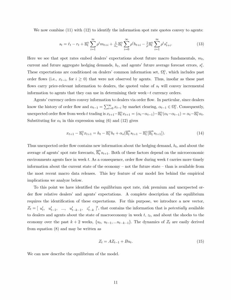
We now combine (11) with (12) to identify the information spot rate quotes convey to agents:

st = rt − rt + Edt∞Xi=1

ρimt+i +1αsEdt

∞Xi=0

ρiht+i − 1ρE

dt

∞Xi=1

ρiset+i. (13)

Here we see that spot rates embed dealers’ expectations about future macro fundamentals, mt,

current and future aggregate hedging demands, ht, and agents’ future average forecast errors, set .

These expectations are conditioned on dealers’ common information set, Ωdt , which includes past

order flows (i.e., xt−i, for i ≥ 0) that were not observed by agents. Thus, insofar as these pastflows carry price-relevant information to dealers, the quoted value of st will convey incremental

information to agents that they can use in determining their week−t currency orders.Agents’ currency orders convey information to dealers via order flow. In particular, since dealers

know the history of order flow and αt−1 =P∞

i=0 xt−i by market clearing, αt−1 ∈ Ωdt . Consequently,unexpected order flow from week-t trading is xt+1−Edt xt+1 = (αt−αt−1)−Edt (αt−αt−1) = αt−Edt αt.Substituting for αt in this expression using (6) and (12) gives

xt+1 − Edt xt+1 = ht − Edt ht + αs(Ent st+1 − Edt [Ent st+1]). (14)

Thus unexpected order flow contains new information about the hedging demand, ht, and about the

average of agents’ spot rate forecasts, Ent st+1. Both of these factors depend on the microeconomicenvironments agents face in week t. As a consequence, order flow during week t carries more timely

information about the current state of the economy — not the future state — than is available from

the most recent macro data releases. This key feature of our model lies behind the empirical

implications we analyze below.

To this point we have identified the equilibrium spot rate, risk premium and unexpected or-

der flow relative dealers’ and agents’ expectations. A complete description of the equilibrium

requires the identification of these expectations. For this purpose, we introduce a new vector,

Zt = [ u0t, u0t−1, ..., u0t−k−1, z0t−k ]0, that contains the information that is potentially available

to dealers and agents about the state of macroeconomy in week t, zt, and about the shocks to the

economy over the past k + 2 weeks, ut, ut−1, ...ut−k−1. The dynamics of Zt are easily derived

from equation (8) and may be written as

Zt = AZt−1 +But. (15)

We can now describe the equilibrium of the model.

11

Proposition In equilibrium, there exists vectors Λs and Λδ such that the log spot rate, risk

premium and unexpected order flow in week-t trading satisfy

st = ΛsEdt Zt, δt = ΛδEdt Zt, (16a)

and xt+1 − Edt xt+1 = αt = αsΛδ(Zt − Edt Zt), (16b)

where Edt Zt = ΦdZt for some matrix Φd, and Zt follows (15).

The Appendix provides a detailed derivation of this proposition. Here we emphasize three

features. First, the equilibrium encompasses the special case where the flow of public information

provides dealers and agents with complete information about the current state of the economy.

This is the information structure found in standard macro exchange rate models. It implies that

Zt = Edt Zt, so dealers can anticipate order flow with complete precision: xt+1 = Edt xt+1. Underthese circumstances, dealers set the risk premium to a level that insures that their foreign currency

holdings are always at their optimal risk-sharing level of zero. And, as a consequence, actual order

flow, xt+1, is also zero. Thus, the presence of incomplete information concerning the current state

of the economy not only accords with reality but is also a necessary condition for the existence of

(non-zero) order flows.

Second, the equilibrium provides a structural explanation for the strong relationship between

high-frequency variations in spot rates and contemporaneous order flows documented by Evans and

Lyons (2002a & 2002b) and many others (see Osler 2008 for a recent survey). According to our

model, this relationship exists because order flows during week t convey information to dealers that

is incorporated into their estimates of potentially available information Zt+1 at the start of week

t+1. More specifically, combining the identity, st+1 = Edt st+1+ (st+1−Edt st+1), with equations (1)and (16a) gives

st+1 − st = rt − rt + δt + Λs(Edt+1 − Edt )Zt+1. (17)

Since the first three terms on the right hand side are known to dealers at the start of week t, changes

in the log spot rate, st+1− st, will be correlated with unexpected order flow, xt+1−Edt xt+1, insofaras the latter is correlated with the revision in dealers’ expectations, (Edt+1−Edt )Zt+1. Evans (2009)

provides a detailed examination of this correlation.

The third feature we wish to emphasize concerns the long run relationship between order flow

and spot rates. Equations (9) and (16b) imply that xt+1 = αsΛδ(Zt − Edt Zt) −αsΛδ(Zt−1 −Edt−1Zt−1), so any permanent shock to an element of Zt has no long-run effect on order flow: The

shock may initially affect elements of Zt − Edt Zt and Zt−1 − Edt−1Zt−1, and so have a short-run

impact; but once dealers learn about its macroeconomic effects, they adjust the risk premium so

that its impact on subsequent order flow vanishes. At the same time, the shock can have a long-run

12

effect on the spot rate. Equation (16a) implies that st = ΛsZt − Λs(Zt − Edt Zt), so a permanent

shock to elements of Zt can affect the spot rate via the first term long after its macroeconomic

impact has been learnt by dealers. In sum, therefore, our model does not imply that there should

be any cointegrating (long-run) relationship between the aggregate flow of agents’ foreign currency

orders cumulated through time and macro variables or the spot rate.

2 Empirical Analysis

In this section we examine the implications of our model for forecasting future macroeconomic

conditions. First we derive a key testable implication of our model regarding the forecasting power

of spot rates and order flow for macro variables. We then describe the data used to estimate these

forecast relationships and present our empirical results.

2.1 Identifying the Forecasting Power of Spot Rates and Order Flow

The forecasting power of spot rates and order flows come from difference sources. Spot rates have

forecasting power in our model because dealers’ quotes include their expectations concerning the

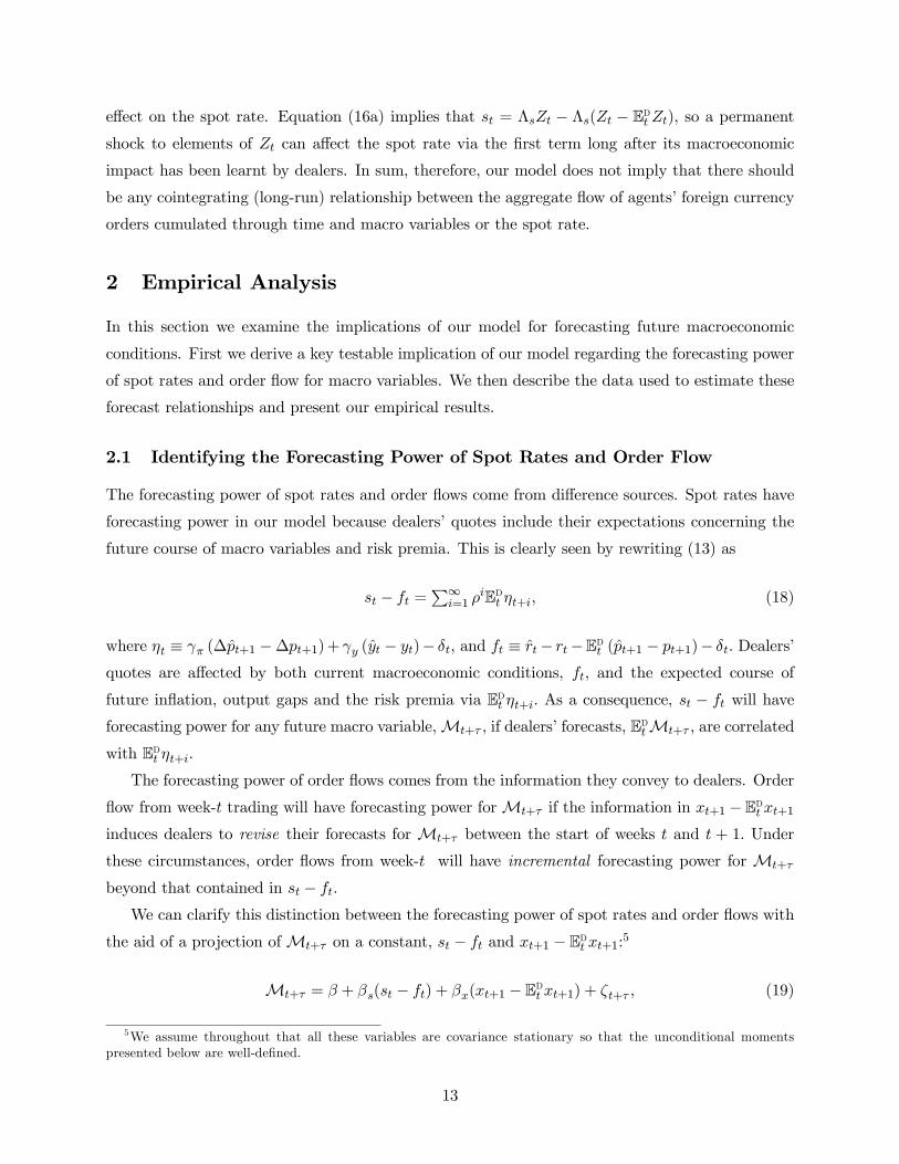
future course of macro variables and risk premia. This is clearly seen by rewriting (13) as

st − ft =P∞

i=1 ρiEdt ηt+i, (18)

where ηt ≡ γπ (∆pt+1 −∆pt+1)+ γy (yt − yt)− δt, and ft ≡ rt− rt−Edt (pt+1 − pt+1)− δt. Dealers’

quotes are affected by both current macroeconomic conditions, ft, and the expected course of

future inflation, output gaps and the risk premia via Edt ηt+i. As a consequence, st − ft will have

forecasting power for any future macro variable,Mt+τ , if dealers’ forecasts, EdtMt+τ , are correlated

with Edt ηt+i.The forecasting power of order flows comes from the information they convey to dealers. Order

flow from week-t trading will have forecasting power forMt+τ if the information in xt+1 −Edt xt+1induces dealers to revise their forecasts for Mt+τ between the start of weeks t and t + 1. Under

these circumstances, order flows from week-t will have incremental forecasting power for Mt+τ

beyond that contained in st − ft.

We can clarify this distinction between the forecasting power of spot rates and order flows with

the aid of a projection ofMt+τ on a constant, st − ft and xt+1 − Edt xt+1:5

Mt+τ = β + βs(st − ft) + βx(xt+1 − Edt xt+1) + ζt+τ , (19)

5We assume throughout that all these variables are covariance stationary so that the unconditional moments

presented below are well-defined.

13

where ζt+τ is the mean-zero projection error that identifies the component ofMt+τ that is uncor-

related with both st − ft and xt+1 − Edt xt+1. Since these terms are uncorrelated with each other,the projection coefficients are given by

βs =CV(Mt+τ , st − ft)

V(st − ft)and βx =

CV(Mt+τ , xt+1 − Edt xt+1)V(xt+1 − Edt xt+1)

, (20)

where CV(., .) and V(.) denote the unconditional covariance and variance operators, respectively.Combining these expressions with (18) and the identity Mt+τ = EdtMt+τ + (Edt+1 − Edt )Mt+τ +

(1− Edt+1)Mt+τ gives

βs =CV(EdtMt+τ ,

P∞i=i ρ

iEdt ηt+i)V(st − ft)

and βx =CV((Edt+1 − Edt )Mt+τ , xt+1 − Edt xt+1)

V(xt+1 − Edt xt+1).

(21)

To interpret the expressions in (21), recall that ρ = 1/(1+γε) where γε identifies the sensitivity

of the expected interest differential, Edt (rt+i−rt+i), to variations in the expected real exchange rate,Edt εt+i. Plausible values for γε should be positive but small (Clarida, Galı, and Gertler 1998), so ρshould be close to one. This being the case, the expression for βs indicates that st − ft will have

greater forecasting power when dealer expectations, EdtMt+τ , are strongly correlated with their

forecasts for expected inflation and/or output gaps over long horizons. In contrast, the expression

for βx shows that the forecasting power of order flow only depends on the information it conveys to

dealers concerningMt+τ . Recall from (14) that xt+1 − Edt xt+1 conveys information about ht andEnt st+1 — two factors that embed more timely information about the current state of the economythan is available to dealers from other sources. The expression for βx shows that order flows will

have incremental forecasting power when dealers find this information relevant for forecasting the

future course ofMt.

The preceding discussion suggests that we empirically investigate the forecasting power of spot

rates and order flows for a macro variableMt by estimating βs and βx from a regression ofMt+τ

on a constant, st − ft and xt+1 − Edt xt+1. Of course, to implement this approach we need dataon these variables over a sufficiently long time span to estimate the moments in βs and βx with

precision. Unfortunately, this is unlikely to be the case in practice. Our data on order flows

covers six an a half years — a longer time span than any other comparable data set — but it does

not contain many observations on standard macro variables such as output and inflation across a

variety of macroeconomic conditions. Consequently, the available time series on Mt, st − ft and

xt+1 − Edt xt+1 are unlikely to have must statistical power for detecting the true values of βs andβx. To address this problem, we implement a novel procedure that estimates the components of βs

and βx.

Let Ωt ⊂ Ωdt denote a subset of the information available to dealers at the start of week t that

14

includesMt. Without loss of generality we can write

Mt+τ =Xτ−1

i=−t Et+i + E[Mt+τ ],

where Et = E[Mt+τ |Ωt+1] − E[Mt+τ |Ωt] is the week-t flow of information into Ωt+1 concerning

Mt+τ , and E[Mt+τ ] = E[Mt+τ |Ω0] denotes the unconditional expectation. Substituting this ex-pression into (20) gives

βs =Xτ−1

i=−t βis and βx =

Xτ−1i=−t β

ix, (22)

where βis and βix are the coefficients from the projection:

Et+i = βi + βis(st − ft) + βix(xt+1 − Edt xt+1) + ξt+i. (23)

Our strategy is to estimate this projection for different horizons i using estimates of Et obtainedfrom a time series model (described below). Unlike the underlying macro time series, Mt, these

estimates can be computed at a high enough frequency for us to estimate βis and βix with precision

given the time span of our data. Of course, this increase in precision comes at a cost. Statistically

significant estimates of βis and βix imply that st − ft and xt+1 −Edt xt+1 have forecasting power forthe flow of information used to revise future expectations concerningMt+τ . However, (22) shows

that this must be true at some horizon(s), i, if st − ft and xt+1 − Edt xt+1 truly have forecastingpower forMt+τ . In sum, therefore, when we test the statistical significance of horizon-specific β

is

and βix we are examining a necessary condition for the existence of forecasting power in spot rates

and order flows.

To implement our procedure, two data issues need addressing. Since (23) includes unanticipated

order flow, xt+1 − Edt xt+1, it appears that we need data on both xt+1 and dealers’ information,

Ωdt , in order to estimate βix. Fortunately, an implication of our model makes this unnecessary.

Recall that dealers choose the risk premium such that Edt αt = 0, and xt+1 − Edt xt+1 = αt − Edt αtbecause αt−1 ∈ Ωdt . Combining these expressions with the market clearing condition in (9) givesxt+1−Edt xt+1 =

P∞i=0 xt+1−i. Thus, the requirement of efficient risk-sharing on the dealers’ choice

of risk premium implies that unexpected order flow can be identified from the cumulation of current

and past order flows, xt+1. The second issue concerns the identification of the macro information

flows, Et+i. We discuss this in the next subsection.

15

2.2 Data

Our empirical analysis uses a data set that includes end-user transaction flows, spot rates, interest

rates and macro fundamentals over six and a half years. The transaction flow data differ in two

important respects from the data used in earlier work (e.g., Evans and Lyons 2002a & 2002b).

First, they cover a much longer time period; January 1993 to June 1999. Second, they come from

transactions between end-users and a large bank, rather than from inter-bank transactions. Our

data cover transactions with three end-user segments: non-financial corporations, investors (such

as mutual funds and pension funds), and leveraged traders (such as hedge funds and proprietary

traders). The data set also contains information on trading location, US versus Non-US. From this

we construct order flows for six segments: trades executed in the US and non-US for non-financial

firms, investors, and leveraged traders. Though inter-bank transactions accounted for about two-

thirds of total volume in major currency markets at the time, they are largely derivative of the

underlying shifts in end-user currency demands. Our data include all the end-user trades with

Citibank in the largest spot market, the USD/EUR market, and the USD/EUR forward market.6

Citibank had the largest share of the end-user market in these currencies at the time, ranging

between 10 and 15 percent. The flow data are aggregated at the daily frequency and measure in

$m the imbalance between end-user orders to purchase and sell euros.

There are many advantages of our transaction flow data. First, the data are simply more

powerful, covering a much longer time span. Second, because the underlying trades reflect the

world economy’s primitive currency demands, the data provide a bridge to modern macro analysis.

Third, the three segments span the full set of underlying demand types. We shall see that those

not covered by extant end-user data sets are empirically important.7

In the analysis that follows we consider the joint behavior of exchange rates and order flows at

the weekly frequency. The weekly timing of the variables is as follows: We take the log spot rate at

the start of week t, denoted by st, to be the log of the offer rate (USD/EUR) quoted by Citibank at

what is generally the end of active trading on Friday of week t−1 (approximately 17:00 GMT). Thisis also the point at which we sample the week−t interest rates from Datastream. In our analysis

6Before January 1999, data for the Euro are synthesized from data in the underlying markets against the Dollar,

using weights of the underlying currencies in the Euro. Data on end-user transactions are only available from

Citibank in this synthesized form, so we cannot study the end-user transactions in individual currencies. That said,

transactions before 1999 are dominated by transactions in the Deutschemark/Dollar. Evans and Lyons (2002a) found

that 87% of the market-wide interdealer transactions between the Dollar and the underlying currencies in the Euro

involved trades in the Deutschemark/Dollar. This study also showed that Deutschemark/Dollar order flow was the

most significant determinant of daily spot rate changes in the other underlying currencies. Furthermore, the weekly

rates of depreciation in the individual currency/Dollar pairs are highly correlated with the weekly depreciation in the

Deutschemark/Dollar between January 1993 to December 1998: the median correlation is 0.95.7Froot and Ramadorai (2005) consider the transactions flows associated with portfolio changes undertaken by

institutional investors. Osler (2003) examines end-user stop-loss orders.

16

below depreciation rates and interest rates are expressed in annual percentage terms. The week-t

flow from segment j, xj, is computed as the total value in $m of euro purchases initiated by the

segment against Citibank’s quotes between the 17:00 GMT on Friday of week t− 1 and Friday ofweek t. Positive values for these order flows therefore denote net demand for euros.

Table 1: Order Flow Summary Statistics

Corporate Hedge Investor

US Non-US US Non-US US Non-US

A:

Mean -16 .8 -59 .8 -4 .1 11 .2 19 .4 15 .9

Standard Deviation 108 .7 196 .1 346 .3 183 .4 146 .6 273 .4

Autocorrelations

ρ1 -0 .037 0 .072 -0 .021 -0 .098 0 .096 0 .061

ρ2 -0 .040 0 .089 0 .024 0 .024 -0 .024 0 .107

ρ4 0 .028 -0 .038 0 .126 0 .015 -0 .030 -0 .030

ρ8 -0 .028 0 .103 -0 .009 0 .083 -0 .016 -0 .014

B: Cross-Correlations

Corporate Non-US -0 .084∗

Traders US 0 .125∗∗ -0 .136∗∗

Traders Non-Us 0 .035 -0 .026 0 .066

Investors US -0 .158∗∗ 0 .035 0 .045 0 .083∗

Investors Non-US -0 .029 -0 .063 0 .159∗∗ -0 .032 0 .094∗

Notes: The table reports weekly-frequency statistics for order flows from end-user segments cumu-

lated over the week between January 1993 and June 1999. The last four rows of panel A report

autocorrelations ρi at lag i. Statistical significance for the cross-correlations at the 10% and 5%

levels is denoted by “∗” and “∗∗”.

Summary statistics for the weekly order flow data are reported in Table 1. The statistics in

panel A display two noteworthy features. First, the order flows are large and volatile. Second, they

display no significant serial correlation. At the weekly frequency, then, the end-user flows appear

to represent shocks to the foreign exchange market arriving at Citibank. Panel B reports the

cross-correlations between the six flows. These correlations are generally quite small, ranging from

approximately -0.16 to 0.16, but several are statistically significant at the 5 percent level. Insofar

as these order flows convey information to dealers, individual segments should not be viewed as

carrying entirely separate information.

We consider the forecasting power of spot rates and order flows for three standard variables,

17

GDP growth, CPI inflation, and M1 growth, both in the US and Germany.8 The flow of macro

information for each of these variables is identified using the real-time estimation method developed

in Evans (2005). To understand how these information flows are estimated, let Mq(i) denote US

GDP growth in quarter i that ends on day q(i) and let Rd denote the vector of scheduled US macro

data releases on day d. The individual data releases in Rd vary from day to day, but the identity

of upcoming releases is known in advance because release dates for each variable follow a preset

schedule. Rd includes monthly series like Nonfarm Payroll as well as the “Advance”, “Preliminary”

and “Final” GDP data for quarter i that are released on three days after q(i).

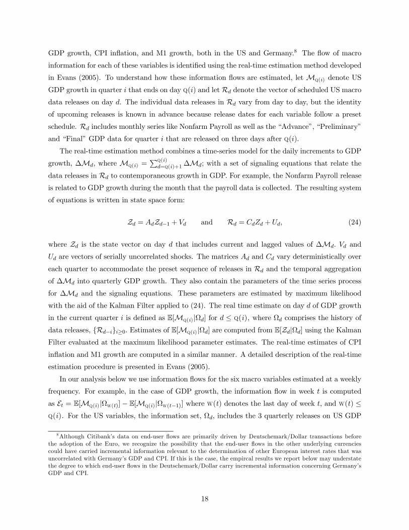
The real-time estimation method combines a time-series model for the daily increments to GDP

growth, ∆Md, where Mq(i) =Pq(i)

d=q(i)+1∆Md; with a set of signaling equations that relate the

data releases in Rd to contemporaneous growth in GDP. For example, the Nonfarm Payroll release

is related to GDP growth during the month that the payroll data is collected. The resulting system

of equations is written in state space form:

Zd = AdZd−1 + Vd and Rd = CdZd + Ud, (24)

where Zd is the state vector on day d that includes current and lagged values of ∆Md. Vd and

Ud are vectors of serially uncorrelated shocks. The matrices Ad and Cd vary deterministically over

each quarter to accommodate the preset sequence of releases in Rd and the temporal aggregation

of ∆Md into quarterly GDP growth. They also contain the parameters of the time series process

for ∆Md and the signaling equations. These parameters are estimated by maximum likelihood

with the aid of the Kalman Filter applied to (24). The real time estimate on day d of GDP growth

in the current quarter i is defined as E[Mq(i)|Ωd] for d ≤ q(i), where Ωd comprises the history ofdata releases, Rd−ii≥0. Estimates of E[Mq(i)|Ωd] are computed from E[Zd|Ωd] using the KalmanFilter evaluated at the maximum likelihood parameter estimates. The real-time estimates of CPI

inflation and M1 growth are computed in a similar manner. A detailed description of the real-time

estimation procedure is presented in Evans (2005).

In our analysis below we use information flows for the six macro variables estimated at a weekly

frequency. For example, in the case of GDP growth, the information flow in week t is computed

as Et = E[Mq(i)|Ωw(t)]− E[Mq(i)|Ωw(t−1)] where w(t) denotes the last day of week t, and w(t) ≤q(i). For the US variables, the information set, Ωd, includes the 3 quarterly releases on US GDP

8Although Citibank’s data on end-user flows are primarily driven by Deutschemark/Dollar transactions before

the adoption of the Euro, we recognize the possibility that the end-user flows in the other underlying currencies

could have carried incremental information relevant to the determination of other European interest rates that was

uncorrelated with Germany’s GDP and CPI. If this is the case, the empircal results we report below may understate

the degree to which end-user flows in the Deutschemark/Dollar carry incremental information concerning Germany’s

GDP and CPI.

18

and the monthly releases on 20 other US macro variables. The information flows for the German

variables are computed using a specification for Ωd that includes the 3 quarterly release on German

GDP and the monthly releases on 8 German macro variables.9 All series come from a database

maintained by Money Market News Services (M.M.S.) that contains details of each data release.

Notice that the information flows we compute use specifications for Ωd that make Ωw(t−1) a subset

of the information available to dealers at the start of week t.

The statistical properties of the macro information flows are summarized in Table 2. Panel

A shows that all the information flows have sample means close to zero and display little serial

correlation. None of the autocorrelations are significant at the 5 percent level. Panel B reports

the cross-correlations between the six information flows. Because the three US (German) flows

are computed from the same set of US (German) data releases, it is not surprising to see some

significant correlations between the US flows and between the German flows. However, none of the

cross correlations are particularly large. This signifies that the data releases convey information

with different relevance for different variables. For example, the Nonfarm Payroll release may

induce a significant revision in the real-time estimate of GDP growth but have little impact on

the real-time estimate of inflation. From this perspective, it appears that our six information flows

convey distinctly different macro information.

To address the statistical power of our resulting information flow series, we compare each series’

power to forecast its own subsequent data release to a forecast from professional money managers.

On the Friday before each scheduled data release, M.M.S. surveys approximately forty money

managers on their estimate for the upcoming release. We computed the forecast error implied by

the median response from the survey asMr − Es[Mr], whereMr is the value released on day r

and Es[Mr] is the median forecast from the survey conducted on day s (< r). The comparable

forecast error using the real-time estimates is computed asMr − E[Mr|Ωs]. The mean and meansquare error for both sets of forecasts errors are reported in Panel C of Table 2. These statistics

show that the forecast errors implied by our estimated conditional expectations are comparable to

those based on the M.M.S. survey. This finding provides assurance that the macro information

flows are not dominated by specification error.

9The real-time estimates for US variables use data releases on: quarterly GDP, Nonfarm Payroll, Employment,

Retail Sales, Industrial Production, Capacity Utilization, Personal Income, Consumer Credit, Personal Consumption

Expenditures, New Home Sales, Durable Goods Orders, Construction Spending, Factory Orders, Business Inventories,

the Government Budget Deficit, the Trade Balance, NAPM index, Housing Starts, the Index of Leading Indicators,

Consumer Prices and M1. The real-time estimates for German variables use data releases on GDP, Employment,

Retail Sales, Industrial Production, Manufacturing Output, Manufacturing Orders, the Trade Balance, Consumer

Prices and M1.

19

Table 2: Summary Statistics for Macro Information Flows

US German

GDP Inflation M1 GDP Inflation M1

A:

Mean <0 .001 <0 .001 -0.006 0 .002 0 .002 0.022

Standard Deviation 0.200 0 .030 1.379 0 .526 0 .806 1.454

Autocorrelations

ρ1 0 .044 0 .013 0.071 0 .022 0 .092 0.070

ρ2 0 .103 -0 .019 0.069 -0 .008 0 .021 0.081

ρ3 0 .007 -0 .004 0.039 -0 .024 -0 .029 0.125

ρ4 0 .019 0 .018 0.015 -0 .026 -0 .049 0.133

B: Cross Correlations

-0 .047

0 .120∗∗ 0 .048

0 .005 -0 .040 0.024

0 .023 -0 .034 0.073∗ 0 .413∗∗

0 .006 0 .046 0.020 -0 .141∗∗ -0 .112∗∗

C: Forecast Comparisons

M.M.S Mean 0.729 -0 .327 0.399 0 .132 -0 .136 4.778

M.M.S. M.S.E 1.310 1 .797 11.807 6 .981 1 .687 42.363

Real-Time Mean 0.190 0 .054 0.033 -0 .416 -0 .035 -0.159

Real-Time M.S.E. 1 .407 2 .357 11.932 6 .954 1 .906 20.561

Notes: The table reports statistics for the macro information flows concerning US GDP growth,

CPI inflation, and M1 growth, and German GDP growth, CPI Inflation, and M1 growth at the

weekly frequency between January 1993 and June 1999; 335 weekly observations. The last four

rows of Panel A report autocorrelations ρi at lag i. Panel C compares the mean and Mean SquaredError (M.S.E.) of real-time estimates against the real-time errors computed from M.M.S. surveys of

professional money managers. Statistical significance at the 10% and 5% level is denoted by ∗ and∗∗, respectively.

2.3 Empirical Results

2.3.1 Macro Forecasting

We begin by examining the forecasting power of spot rates for the six macro information flows. In

our model it is the difference between the current spot rate and fundamentals, st−ft, that identifiesthe potential forecasting power of spot rates. We proxy this difference with the depreciation rate,

∆st, and four interest rate spreads: the US default, commercial paper and term spreads and the

German term spread. The US and German term spreads, sptt and bsptt , are computed as thedifference between the 3-month and 5-year yields on government bonds. We compute the US

default spread, spdt as the difference between Moody’s AAA corporate bond yield and Moody’s

20

BAA corporate bond yield. The US commercial paper spread, spcpt , is the difference between the

3-month commercial paper rate and the 3-month T-Bill rate. Before September 1997 we use the

3-month commercial paper rate, thereafter the 3-month rate for non-financial corporations. The

spreads are computed from the interests rates on Friday of week t−1, and so represent informationthat was available to dealers at the start of week t: if they have forecasting power for the macro

information flows, dealers should have been able to forecast these macro flows at the time.

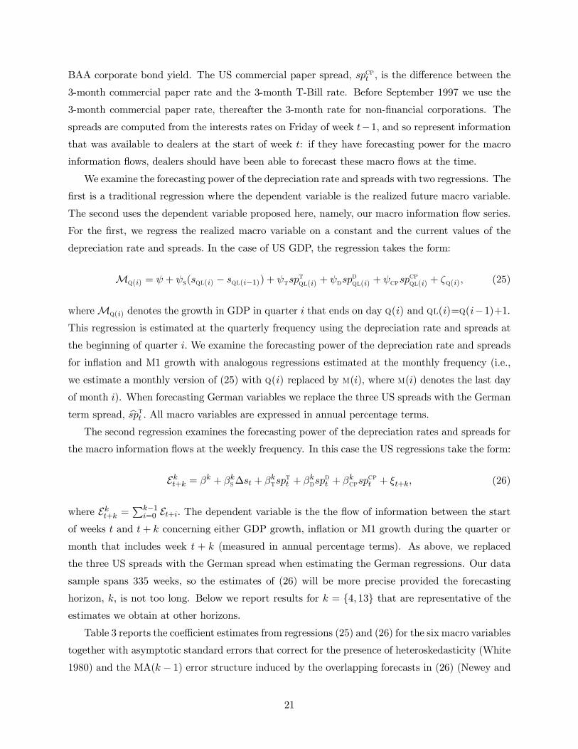
We examine the forecasting power of the depreciation rate and spreads with two regressions. The

first is a traditional regression where the dependent variable is the realized future macro variable.

The second uses the dependent variable proposed here, namely, our macro information flow series.

For the first, we regress the realized macro variable on a constant and the current values of the

depreciation rate and spreads. In the case of US GDP, the regression takes the form:

Mq(i) = ψ + ψs(sql(i) − sql(i−1)) + ψtsptql(i) + ψdsp

dql(i) + ψcpsp

cpql(i) + ζq(i), (25)

whereMq(i) denotes the growth in GDP in quarter i that ends on day q(i) and ql(i)=q(i−1)+1.This regression is estimated at the quarterly frequency using the depreciation rate and spreads at

the beginning of quarter i. We examine the forecasting power of the depreciation rate and spreads

for inflation and M1 growth with analogous regressions estimated at the monthly frequency (i.e.,

we estimate a monthly version of (25) with q(i) replaced by m(i), where m(i) denotes the last day

of month i). When forecasting German variables we replace the three US spreads with the German

term spread, bsptt . All macro variables are expressed in annual percentage terms.The second regression examines the forecasting power of the depreciation rates and spreads for

the macro information flows at the weekly frequency. In this case the US regressions take the form:

Ekt+k = βk + βks∆st + βktsptt + βkdsp

dt + βkcpsp

cpt + ξt+k, (26)

where Ekt+k =Pk−1

i=0 Et+i. The dependent variable is the the flow of information between the startof weeks t and t+ k concerning either GDP growth, inflation or M1 growth during the quarter or

month that includes week t + k (measured in annual percentage terms). As above, we replaced

the three US spreads with the German spread when estimating the German regressions. Our data

sample spans 335 weeks, so the estimates of (26) will be more precise provided the forecasting

horizon, k, is not too long. Below we report results for k = 4, 13 that are representative of theestimates we obtain at other horizons.

Table 3 reports the coefficient estimates from regressions (25) and (26) for the six macro variables

together with asymptotic standard errors that correct for the presence of heteroskedasticity (White

1980) and the MA(k − 1) error structure induced by the overlapping forecasts in (26) (Newey and

21

Table 3: Forecasting Macro Information Flows

US German

∆s spd spt spcp R2 ∆s spt R2

A: GDP Growth

(i) -0 .552 -6 .855∗∗∗ 0 .386 2.097 0 .274 -5.688 3 .267∗∗ 0 .25

(0 .574) (2 .333) (0 .333) (1.880) (10.736) (1 .332)

(ii) k = 4 -0 .018 -0 .357∗ 0 .035 0.296∗∗∗ 0 .066 -0.266∗∗∗ 0 .259∗∗ 0 .11

(0 .029) (0 .189) (0 .025) (0.087) (0.076) (0 .115)

(iii) k = 13 -0 .049 -0 .298∗∗∗ 0 .025 0.201∗∗∗ 0 .125 -0.014 0 .266∗∗∗ 0 .19

(0 .050) (0 .101) (0 .022) (0.072) (0.092) (0 .059)

B: Inflation

(i) -0 .072 0 .046 0 .024 0.073 0 .033 -2.989 -0 .917 0 .07

(0 .073) (0 .131) (0 .017) (0.072) (10.010) (0 .641)

(ii) k = 4 0 .343 -0 .698 0 .448 -1.659 0 .029 -0.443∗∗∗ -0 .088 0 .09

(0 .344) (3 .014) (0 .342) (1.485) (0.124) (0 .143)

(iii) k = 13 0 .832 -0 .639 0 .397 -1.664 0 .085 0.058 -0 .118 0 .01

(0 .641) (2 .350) (0 .326) (1.176) (0.168) (0 .135)

C: M1 Growth

(i) 0 .732 -14 .736∗∗ 1 .176∗ -0 .969 0 .163 -0.135 -6 .243∗∗∗ 0 .38

(3 .823) (7 .331) (0 .696) (3.881) (1.867) (1 .367)

(ii) k = 4 -7 .042 -4 .947∗∗∗ 0 .415∗∗∗ -0 .329 0 .162 0.039 -1 .385∗∗∗ 0 .16

(4 .634) (1 .283) (0 .143) (0.888) (0.179) (0 .431)

(iii) k = 13 2 .662 -4 .466∗∗ 0 .314∗ -0 .359 0 .217 -0.249 -1 .686∗∗∗ 0 .47

(3 .134) (1 .200) (0 .181) (0.976) (0.343) (0 .342)

Notes: The table reports OLS estimates of regression (25) in line (i) and regression (26) in lines (ii)

and (iii). In line (i) the dependent variable is GDP growth over the next quarter (panel A), inflation

over the next month (panel B) and M1 growth over the next month (panel C). In lines (ii) and (iii)

the dependent variables are the macro information flows over k weeks concerning future GDP growth(panel A), inflation (panel B) and M1 growth (panel C). The left and right hand columns report

estimates using US variables and German variables, respectively. The column headers show the

regressors in each regression. Asymptotic standard errors are reported in parenthesis corrected for

heteroskedasticity (line i) and both heteroskedasticity and MA(k−1) serial correlation (lines ii andiii). Statistical significance at the 10%, 5% and 1% levels is denoted by ∗, ∗∗ and ∗∗∗, respectively.

West 1987). The table displays three noteworthy features. First, there is strong evidence in Panel

A that dealers had access to information with forecasting power for real GDP growth in both the

US and Germany. While the estimates of (25) in row (i) are based on just 24 observations and

so should be interpreted with caution, the estimates of (26) in rows (ii) and (iii) can be reliably

interpreted as indicating that dealers had access to information with forecasting power for both

US and German GDP growth. In particular, the estimates indicate that spdt , spcpt and bsptt have

significant forecasting power for the flows of future macro information concerning GDP growth over

the next month (k = 4) and quarter (k = 13). The estimates in panel C indicate that the spreads

22

have similar significant forecasting power for information flows concerning M1 growth. The second

feature concerns the forecastability of inflation. In contrast to panels A and C, only one of the

coefficient estimates in panel B is statistically significant. Furthermore, all of the regression R2

statistics are much smaller than their counterparts in the other panels. Since spreads are known

to have forecasting power for future inflation in other periods (e.g., Mishkin 1990), we attribute

these findings to the relative stability of inflation in our data sample. Finally, we note that the

depreciation rate has significant forecasting power for the information flows concerning just German

GDP growth and inflation. Clearly, dealers have access to much more precise information about

the future course of GDP and M1 growth than is indicated by depreciation rates alone.

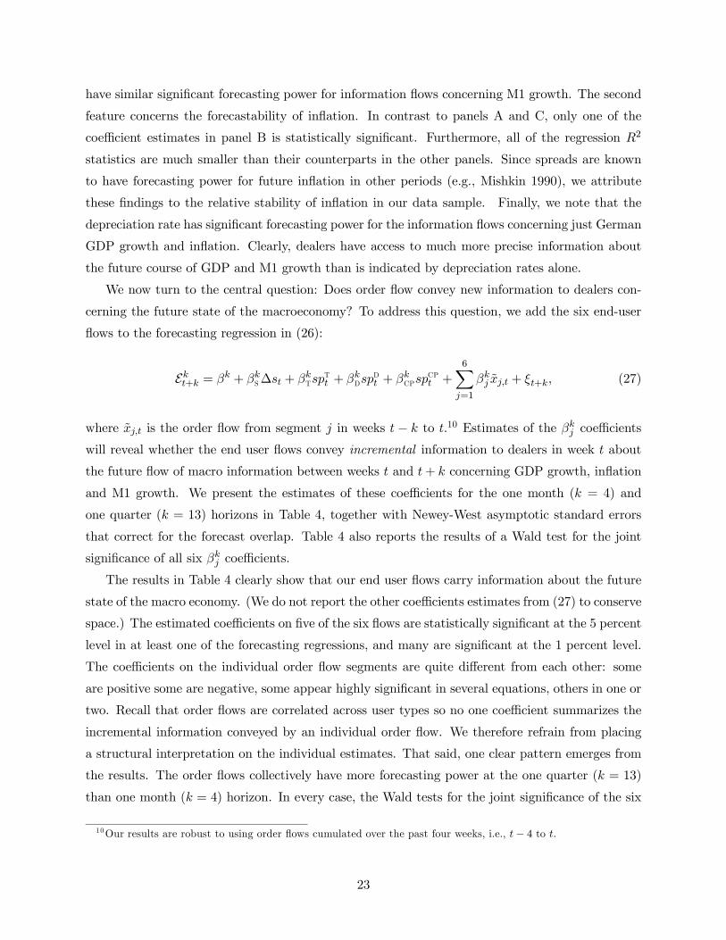
We now turn to the central question: Does order flow convey new information to dealers con-

cerning the future state of the macroeconomy? To address this question, we add the six end-user

flows to the forecasting regression in (26):

Ekt+k = βk + βks∆st + βktsptt + βkdsp

dt + βkcpsp

cpt +

6Xj=1

βkj xj,t + ξt+k, (27)

where xj,t is the order flow from segment j in weeks t − k to t.10 Estimates of the βkj coefficients

will reveal whether the end user flows convey incremental information to dealers in week t about

the future flow of macro information between weeks t and t+ k concerning GDP growth, inflation

and M1 growth. We present the estimates of these coefficients for the one month (k = 4) and

one quarter (k = 13) horizons in Table 4, together with Newey-West asymptotic standard errors

that correct for the forecast overlap. Table 4 also reports the results of a Wald test for the joint

significance of all six βkj coefficients.

The results in Table 4 clearly show that our end user flows carry information about the future

state of the macro economy. (We do not report the other coefficients estimates from (27) to conserve

space.) The estimated coefficients on five of the six flows are statistically significant at the 5 percent

level in at least one of the forecasting regressions, and many are significant at the 1 percent level.

The coefficients on the individual order flow segments are quite different from each other: some

are positive some are negative, some appear highly significant in several equations, others in one or

two. Recall that order flows are correlated across user types so no one coefficient summarizes the

incremental information conveyed by an individual order flow. We therefore refrain from placing

a structural interpretation on the individual estimates. That said, one clear pattern emerges from

the results. The order flows collectively have more forecasting power at the one quarter (k = 13)

than one month (k = 4) horizon. In every case, the Wald tests for the joint significance of the six

10Our results are robust to using order flows cumulated over the past four weeks, i.e., t− 4 to t.

23

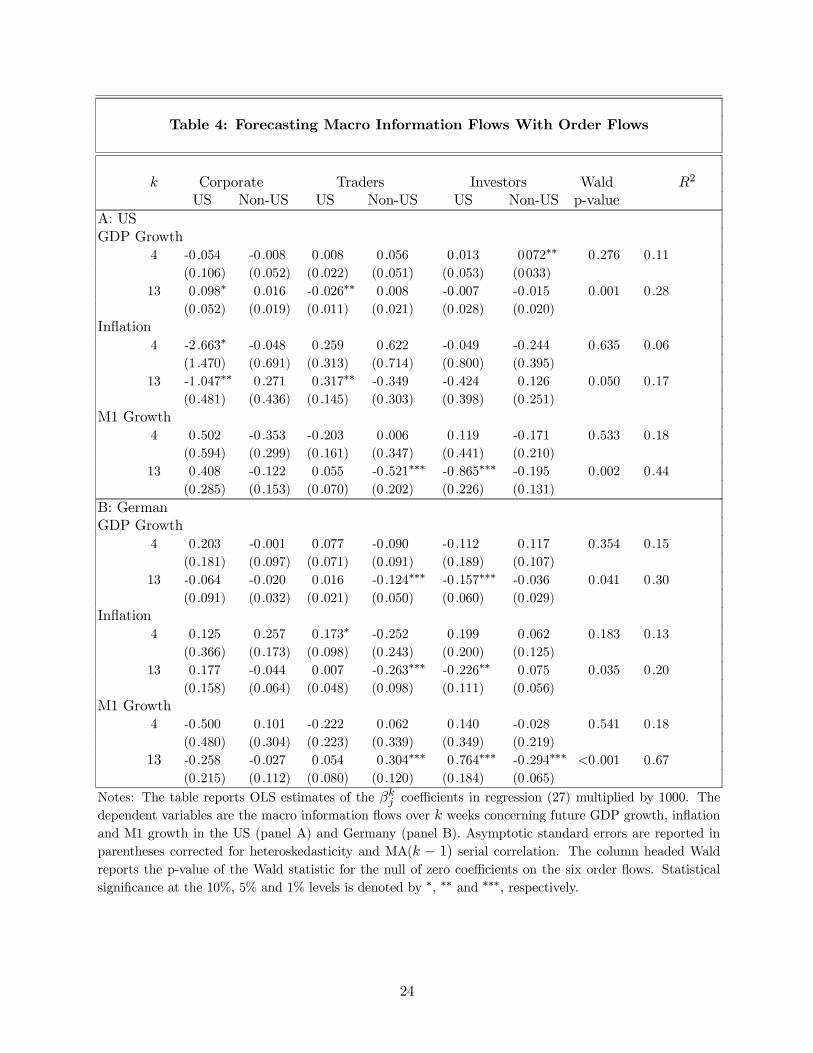
Table 4: Forecasting Macro Information Flows With Order Flows

k Corporate Traders Investors Wald R2

US Non-US US Non-US US Non-US p-value

A: US

GDP Growth

4 -0 .054 -0 .008 0 .008 0 .056 0 .013 0072∗∗ 0.276 0.11

(0 .106) (0 .052) (0 .022) (0 .051) (0 .053) (0033)

13 0 .098∗ 0 .016 -0 .026∗∗ 0 .008 -0 .007 -0.015 0.001 0.28

(0 .052) (0 .019) (0 .011) (0 .021) (0 .028) (0.020)

Inflation

4 -2 .663∗ -0 .048 0 .259 0 .622 -0 .049 -0.244 0.635 0.06

(1 .470) (0 .691) (0 .313) (0 .714) (0 .800) (0.395)

13 -1 .047∗∗ 0 .271 0 .317∗∗ -0 .349 -0 .424 0.126 0.050 0.17

(0 .481) (0 .436) (0 .145) (0 .303) (0 .398) (0.251)

M1 Growth

4 0.502 -0 .353 -0 .203 0 .006 0 .119 -0.171 0.533 0.18

(0 .594) (0 .299) (0 .161) (0 .347) (0 .441) (0.210)

13 0 .408 -0 .122 0 .055 -0 .521∗∗∗ -0 .865∗∗∗ -0 .195 0.002 0.44

(0 .285) (0 .153) (0 .070) (0 .202) (0 .226) (0.131)

B: German

GDP Growth

4 0.203 -0 .001 0 .077 -0 .090 -0 .112 0.117 0.354 0.15

(0 .181) (0 .097) (0 .071) (0 .091) (0 .189) (0.107)

13 -0 .064 -0 .020 0 .016 -0 .124∗∗∗ -0 .157∗∗∗ -0 .036 0.041 0.30

(0 .091) (0 .032) (0 .021) (0 .050) (0 .060) (0.029)

Inflation

4 0 .125 0 .257 0 .173∗ -0 .252 0 .199 0.062 0.183 0.13

(0 .366) (0 .173) (0 .098) (0 .243) (0 .200) (0.125)

13 0 .177 -0 .044 0 .007 -0 .263∗∗∗ -0 .226∗∗ 0.075 0.035 0.20

(0 .158) (0 .064) (0 .048) (0 .098) (0 .111) (0.056)

M1 Growth

4 -0 .500 0 .101 -0 .222 0 .062 0 .140 -0.028 0.541 0.18

(0 .480) (0 .304) (0 .223) (0 .339) (0 .349) (0.219)

13 -0 .258 -0 .027 0 .054 0 .304∗∗∗ 0 .764∗∗∗ -0 .294∗∗∗ <0.001 0.67

(0 .215) (0 .112) (0 .080) (0 .120) (0 .184) (0.065)

Notes: The table reports OLS estimates of the βkj coefficients in regression (27) multiplied by 1000. Thedependent variables are the macro information flows over k weeks concerning future GDP growth, inflationand M1 growth in the US (panel A) and Germany (panel B). Asymptotic standard errors are reported in

parentheses corrected for heteroskedasticity and MA(k − 1) serial correlation. The column headed Waldreports the p-value of the Wald statistic for the null of zero coefficients on the six order flows. Statistical

significance at the 10%, 5% and 1% levels is denoted by ∗, ∗∗ and ∗∗∗, respectively.

24

flow coefficients are significant at the 5 percent level at the quarterly horizon. Furthermore, the R2

statistics in these regressions are on average about twice the size of their counterparts in the Table

3. By this measure, the flows contain an economically significant degree of incremental forecasting

power for the macro information flows beyond that contained in the deprecation rates and spreads.

The incremental forecasting power of the six flow segments extends over a wide range of hori-

zons. To show this, we computed the variance contribution of the flows from the estimates of (27)

for horizons ranging from one week to two quarters. In particular, let Ekt+k = βk+ bEt,∆s+ bEt,x+ ξt+k

denote estimates of (27) where bEt,∆s = βk

s∆st + βk

tsptt + β

k

dspdt + β

k

cpspcpt and bEt,x =P6

j=1 βk

j xj,t.

Multiplying both sides of this expression by Ekt+k and taking expectations gives the following de-composition for the variance of the k-horizon information flow:

V(Ekt+k) = CV(bEt,∆s, Ekt+k) +CV(bEt,x,Ekt+k) +CV(ξt+k, Ekt+k).The contribution of the order flows is given by the second term on the right. We calculated

this contribution as the slope coefficient in the regression of bEt,x on Ekt+k; i.e., an estimate ofCV(bEt,x,Ekt+k)/V(Ekt+k). We also computed the standard error of this estimate with the Newey-West estimator allowing for an MA(k − 1) error process.

Figure 2 plots the variance contributions of the order flows together with 95 percent confidence

bands for the six macro information flows for horizons k = 1, .., 26. In five of the six cases, the

contributions rise steadily with the horizon and are quite sizable beyond one quarter. The exception

is US GDP growth, where the contribution remains around 15 percent from the quarterly horizon

onward. For perspective on these results, recall from Section 2.1 that order flow has incremental

forecasting power for a macro variableMt+τ when the projection coefficient βs =Pτ−1

i=−t βix differs

from zero, where βix measures order flows’ forecasting power for the flow of information at horizon i

concerningMt+τ . The plots in Figure 2 show that order flows have considerable forecasting power

for the future flows of information concerning GDP growth, inflation and M1 growth at all but the

shortest horizons. Clearly, then, these order flows are carrying significant information on future

macroeconomic conditions.

Our analysis to this point has been based on asymptotic inference. To insure that our results

concerning the forecasting power of order flows are robust, we also constructed a bootstrap dis-

tribution for the regression estimates of (27) at the one- and two-quarter horizons (k = 13, 26).11

11Estimates of long-horizon forecasting regressions like (25) and (26) are susceptible to two well-known econometric

problems. First, the coefficient estimates may suffer from finite sample bias when the independent variables are

predetermined but not exogenous. Second, the asymptotic distribution of the estimates provides a poor approximation

to the true distribution when the forecasting horizon is long relative to the span of the sample. Finite-sample bias

in the estimates of βkj is not a prime concern because our six flow segments display little or no autocorrelation

and are uncorrelated with lagged information flows. There should also be less of a size distortion in the asymptotic

25

A: US GDP Growth B: German GDP Growth

C: US Inflation D: German Inflation

E: US M1 Growth F: German M1 Growth

Figure 2: Estimated Contribution of Order Flows to the Variance of Future In-

formation Flows concerning GDP growth, Inflation and M1 growth by forecasting

horizon, τ, measured in weeks. Dashed lines denote 95% percent confidence bands

computed as ±1.96σ, where σ is the standard error of the estimated contribution.

The bootstrap distribution was constructed under the null hypothesis that the order flows have no

incremental forecasting for the macro information flows (see Appendix for details). We found that

the estimated coefficients on the end-user flows are jointly significant at the 5 percent level when

compared against this distribution.

distribution than is found elsewhere. For example, Mark (1995) considered a case where the data span is less than five

times the length of his longest forecasting horizon. Here, we have 11 non-overlapping observations at the 2-quarter

horizon.

26

The results in Table 4 and Figure 2 contrast with the findings of F&R. They found no evi-

dence of a long run correlation between real interest rate differentials and the transaction flows of

institutional investors. As we noted above, this result is completely consistent with our theoretical

model: Order flows can convey information to dealers about macro variables without there being

any long-run statistical relationship between order flow and the variable in question. Our model

also provides perspective on why the incremental forecasting power of order flows could increase

with the horizon. Recall from equation (14) that unexpected order flow, xt+1 − Edt xt+1, containsnew information about the hedging demand, ht, and about the average of agents’ spot rate forecast

series, Ent st+1. Insofar as these two components embed agent’s expectations for monetary policy’sfull future path, they will convey information to dealers about the full future course of output, in-

flation and monetary growth, not simply at short-horizons. We present further evidence consistent

with this interpretation below.12

2.3.2 Macro Information and the Risk Premium

If order flows convey information about future macroeconomic conditions, how do dealers use

this information in determining their spot rate quotes? To address this question, recall that the

equilibrium spot rate follows

st = rt − rt + Edt∞Pi=1

ρimt+i − Edt∞Pi=0

ρiδt+i,

where mt = γπ (∆pt+1 −∆pt+1) + γy (yt − yt) +1−ρρ (pt − pt). In principle, dealers could use the

information in order flows to revise their forecasts for future macro fundamentals, mt, leaving their

forecasts for the risk premium on the euro, δt, unchanged. This would be consistent with the class

of macro models that treat the risk premium as a constant. Alternatively, dealers may find the

information conveyed by order flow useful for revising their forecasts of both mt and δt. In this case,

order flows should have forecasting power for excess returns. For example, let ert+1 = ∆st+1+rt−rtdenote the log excess return on euros between the start of weeks t and t+1. Combining this definition

with (1) gives

ert+2 = δt+1 + st+2 − Edt+1st+1 = Edt δt+1 + (δt+1 − Edt δt+1) + (st+2 − Edt+1st+1).

12After the first draft of this paper, Evans and Lyons (2004a), began circulating, Rime, Sarno, and Sojli (2007)

reported other forecasting results consistent with our findings. They examined the short-term forecasting power of

aggregate interdealer order flow in the USD/EUR, USD/GBP and USD/JPY markets for specific macro data releases

scheduled in the next week. Their findings are based on a much shorter data sample.

27

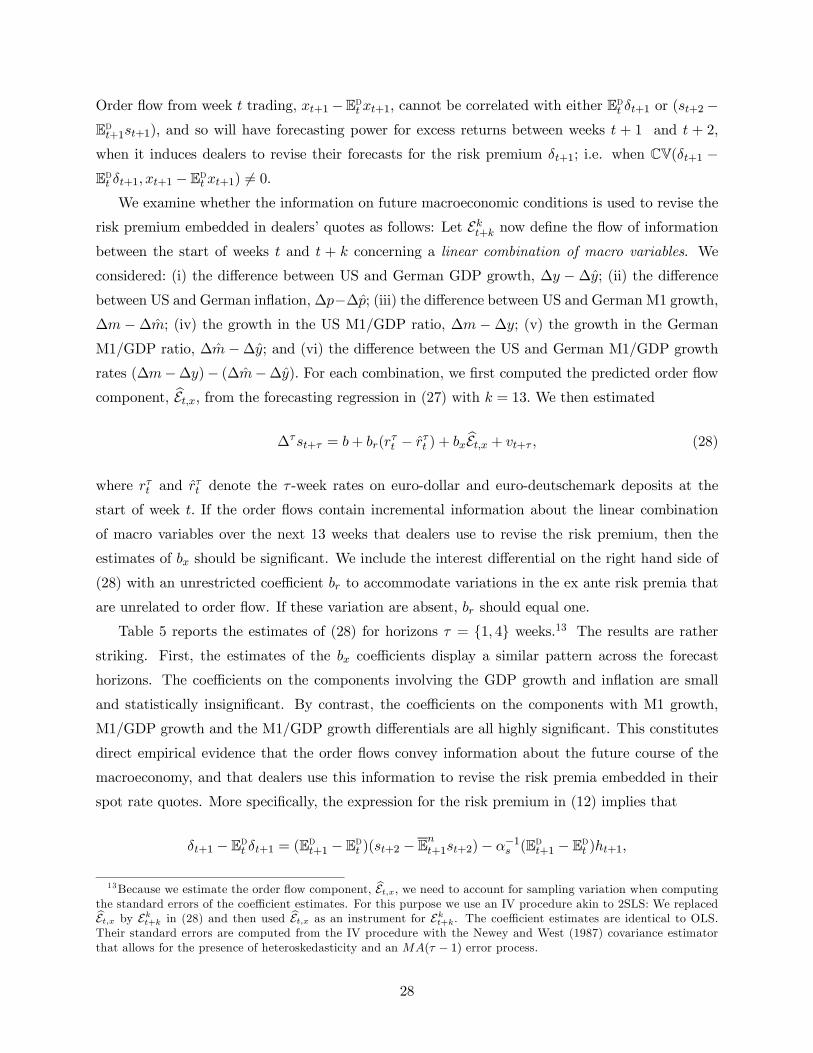
Order flow from week t trading, xt+1−Edt xt+1, cannot be correlated with either Edt δt+1 or (st+2−Edt+1st+1), and so will have forecasting power for excess returns between weeks t + 1 and t + 2,

when it induces dealers to revise their forecasts for the risk premium δt+1; i.e. when CV(δt+1 −Edt δt+1, xt+1 − Edt xt+1) 6= 0.

We examine whether the information on future macroeconomic conditions is used to revise the

risk premium embedded in dealers’ quotes as follows: Let Ekt+k now define the flow of informationbetween the start of weeks t and t + k concerning a linear combination of macro variables. We

considered: (i) the difference between US and German GDP growth, ∆y −∆y; (ii) the differencebetween US and German inflation, ∆p−∆p; (iii) the difference between US and German M1 growth,∆m −∆m; (iv) the growth in the US M1/GDP ratio, ∆m −∆y; (v) the growth in the GermanM1/GDP ratio, ∆m−∆y; and (vi) the difference between the US and German M1/GDP growthrates (∆m−∆y)− (∆m−∆y). For each combination, we first computed the predicted order flowcomponent, bEt,x, from the forecasting regression in (27) with k = 13. We then estimated

∆τst+τ = b+ br(rτt − rτt ) + bx bEt,x + vt+τ , (28)

where rτt and rτt denote the τ -week rates on euro-dollar and euro-deutschemark deposits at the

start of week t. If the order flows contain incremental information about the linear combination

of macro variables over the next 13 weeks that dealers use to revise the risk premium, then the

estimates of bx should be significant. We include the interest differential on the right hand side of

(28) with an unrestricted coefficient br to accommodate variations in the ex ante risk premia that

are unrelated to order flow. If these variation are absent, br should equal one.

Table 5 reports the estimates of (28) for horizons τ = 1, 4 weeks.13 The results are ratherstriking. First, the estimates of the bx coefficients display a similar pattern across the forecast

horizons. The coefficients on the components involving the GDP growth and inflation are small

and statistically insignificant. By contrast, the coefficients on the components with M1 growth,

M1/GDP growth and the M1/GDP growth differentials are all highly significant. This constitutes

direct empirical evidence that the order flows convey information about the future course of the

macroeconomy, and that dealers use this information to revise the risk premia embedded in their

spot rate quotes. More specifically, the expression for the risk premium in (12) implies that

δt+1 − Edt δt+1 = (Edt+1 − Edt )(st+2 − Ent+1st+2)− α−1s (Edt+1 − Edt )ht+1,

13Because we estimate the order flow component, Et,x, we need to account for sampling variation when computingthe standard errors of the coefficient estimates. For this purpose we use an IV procedure akin to 2SLS: We replaced

Et,x by Ekt+k in (28) and then used Et,x as an instrument for Ekt+k. The coefficient estimates are identical to OLS.Their standard errors are computed from the IV procedure with the Newey and West (1987) covariance estimator

that allows for the presence of heteroskedasticity and an MA(τ − 1) error process.

28

so dealers will adjust the risk premium upward when they infer from order flow that on average

agents are underestimating the future depreciation of the dollar by a larger amount; i.e., when

(Edt+1 − Edt )(st+2 − Ent+1st+2) > 0. This will happen, for example, when dealers’ raise their ex-

pectations for the future path of the interest differential, rt+i − rt+i, relative to the average path

expected by agents. In other words, when the information in order flow leads dealers to expect

a looser (tighter) future US (German) monetary policy than the average forecast outside of the

foreign exchange market. Under these circumstances, order flows forecasting looser (tighter) fu-

ture monetary conditions in the US (Germany) should induce dealers to raise the risk premium

on the euro, with the result that the order flows forecast positive future returns on the euro. The

signs of the statistically significant coefficients on the M1/GDP growth components in Table 5 are

consistent with this explanation.

The second noteworthy feature concerns the R2 statistics. They rise from less than 6 percent

to 14 percent as we move from the one week to one month forecasting horizon. By comparison,

the R2 statistics from Fama-style regressions of future returns on the interest differentials alone are

typically less than 3 percent. Here all the forecasting power comes from the order flow component,bEt,x. If (28) is re-estimated without the interest differentials, the bx estimates and R2 statistics are

essentially unchanged. Our results are also robust to imposing br = 1 as a restriction.

Of course, a logical possibility is that dealers revise the risk premium in their spot quotes in

response to order flows, but part of the reason is unrelated to future macroeconomic conditions. If

this is the case, order flows should have forecasting power for future (excess) returns beyond that

found in bEt,x. The right hand column of Table 5 provides statistical evidence on this possibility.Here we report the p-values of LM statistics for the null hypothesis that the residuals from (28)

are unrelated to the six flows. As the table shows, the p-values are well above 5 percent in all the

cases where the estimated bx coefficients appear significant.

The results in Table 5 provide a macro-based explanation for the forecasting results first re-

ported in Evans and Lyons (2005). There we showed that end-user flows had significant out-of-

sample forecasting power for excess currency returns at the four-week horizon.14 Our findings in

Table 5 indicate that this forecasting power stems from the fact that order flows convey significant

information about future macroeconomic conditions, specifically M1 and GDP growth, that deal-

ers use to revise the risk premia they embed in their spot rate quotes. To our knowledge, this is

the first piece of empirical evidence identifying the process by which macroeconomic information

14These findings are consistent with the results of in-sample forecasting tests. In an earlier version of this paper we

showed that Citibank’s order flows forecast euro returns at horizons of two to four weeks with in-sample R2 statistics

of approximately 8 to 16 percent (results available on request). We recognize that the relative merits of in-sample and

out-of-sample evaluation methods are the subject of debate in the econometrics literature (Inoue and Kilian 2005),

but they do not appear important in the present context.

29

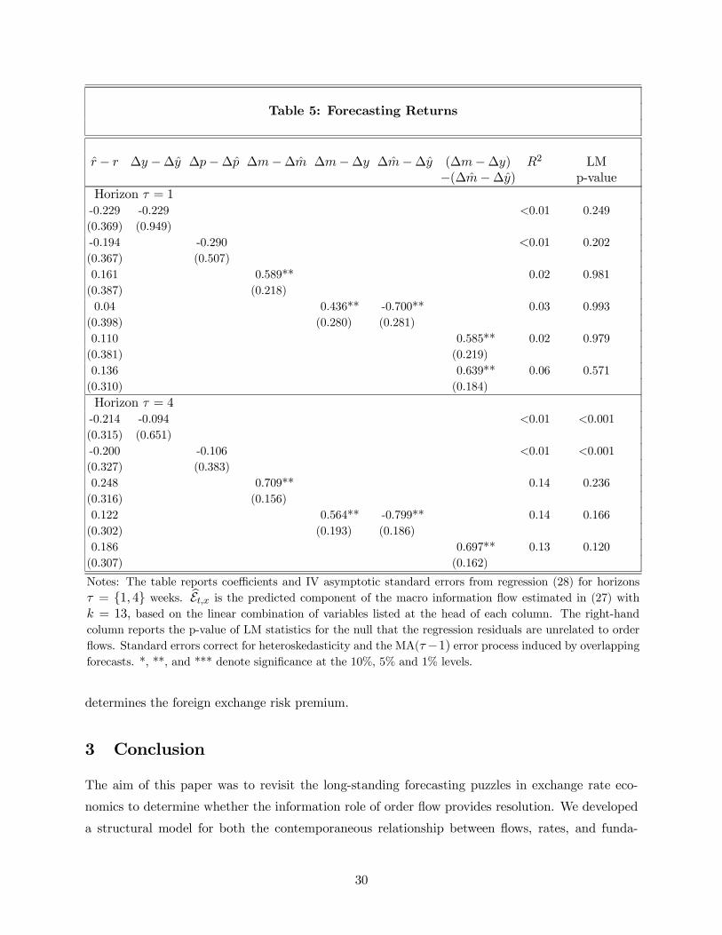
Table 5: Forecasting Returns

r − r ∆y −∆y ∆p−∆p ∆m−∆m ∆m−∆y ∆m−∆y (∆m−∆y) R2 LM

−(∆m−∆y) p-value

Horizon τ = 1-0.229 -0.229 <0.01 0.249

(0.369) (0.949)

-0.194 -0.290 <0.01 0.202

(0.367) (0.507)

0.161 0.589** 0.02 0.981

(0.387) (0.218)

0.04 0.436** -0.700** 0.03 0.993

(0.398) (0.280) (0.281)

0.110 0.585** 0.02 0.979

(0.381) (0.219)

0.136 0.639** 0.06 0.571

(0.310) (0.184)

Horizon τ = 4-0.214 -0.094 <0.01 <0.001

(0.315) (0.651)

-0.200 -0.106 <0.01 <0.001

(0.327) (0.383)

0.248 0.709** 0.14 0.236

(0.316) (0.156)

0.122 0.564** -0.799** 0.14 0.166

(0.302) (0.193) (0.186)

0.186 0.697** 0.13 0.120

(0.307) (0.162)

Notes: The table reports coefficients and IV asymptotic standard errors from regression (28) for horizons

τ = 1, 4 weeks. bEt,x is the predicted component of the macro information flow estimated in (27) withk = 13, based on the linear combination of variables listed at the head of each column. The right-handcolumn reports the p-value of LM statistics for the null that the regression residuals are unrelated to order

flows. Standard errors correct for heteroskedasticity and the MA(τ−1) error process induced by overlappingforecasts. *, **, and *** denote significance at the 10%, 5% and 1% levels.

determines the foreign exchange risk premium.

3 Conclusion

The aim of this paper was to revisit the long-standing forecasting puzzles in exchange rate eco-

nomics to determine whether the information role of order flow provides resolution. We developed

a structural model for both the contemporaneous relationship between flows, rates, and funda-

30

mentals and the implied forecasting relationship. The contemporaneous relationship arises because

transaction flows reveal macroeconomic information that was previously dispersed, and therefore

not fully impounded in the exchange rate. The forecasting relationship arises because the same

macro information revealed by flows is useful for determining the foreign exchange risk premium,

generating rational forecastability in excess returns. We then examined the empirical implica-

tions of the model. We found that transaction flows have significant forecasting power for macro

fundamentals — incremental forecasting power beyond that contained in exchange rates and other

variables. We also showed that transaction flows have significant forecasting power for exchange

rate returns. Our model provides a rational interpretation for these forecastable returns in that

the macro information being revealed by flows is important for determining the foreign exchange

risk premium. In sum, we find strong support for the idea that exchange rates vary as the market

assimilates dispersed macro information from transaction flows.

We conclude with some perspective. Our results provide a qualitatively different view of why

macroeconomic variables perform so poorly in accounting for exchange rates at horizons of one

year or less. This view is different from both the traditional macro and the emerging “micro”

perspectives. Unlike the macro perspective, we do not view all new information concerning macro

fundamentals as being impounded from public-information sources. Much information about macro

fundamentals is initially microeconomically dispersed. The market needs to assimilate implications

for the spot exchange rate, and for other asset prices, via trading. It is this assimilation process

that accounts for (much of) the disturbances in exchange rate equations. Our approach also differs

from the extant micro perspective because models offered thus far (e.g., Evans and Lyons 2002a

&2002b) have interpreted the information conveyed by transaction flows as orthogonal to macro

fundamentals. Most readers of this micro literature have adopted the same view. Our findings, by

contrast, suggest that transaction flows are central to the process of impounding information into

exchange rates. In particular, they point to the existence of a transaction-mediated link between

the foreign exchange risk premium and the macroeconomy that is new to the literature. In light

of the long-standing difficulty of relating excess currency returns to conventional measures of risk

(see Burnside, Eichenbaum, Kleshchelski, Rebelo, Hall, and Hall 2008 for a recent contribution),

exploring this link should be a high priority for future exchange rate research.

References

Bacchetta, P. and E. van Wincoop (2006). Can information heterogeneity explain the exchange

rate determination puzzle? American Economic Review 96 (3), 552—576.

Burnside, A., M. Eichenbaum, I. Kleshchelski, S. Rebelo, L. Hall, and H. Hall (2008). Do Peso

31

Problems Explain the Returns to the Carry Trade? NBER Working Paper .

Cheung, Y., M. Chinn, and A. Pascual (2005). Empirical exchange rate models of the nineties:

Are any fit to survive? Journal of International Money and Finance 24 (7), 1150—1175.

Clarida, R., J. Galı, and M. Gertler (1998). Monetary policy rules in practice some international

evidence. European Economic Review 42 (6), 1033—1067.

Devereux, M. and A. Sutherland (2006). Solving for Country Portfolios in Open Economy Macro

Models.

Engel, C., N. Mark, and K. West (2007). Exchange Rate Models are Not as Bad as You Think.

NBER Working Paper .

Engel, C. and K. West (2006). Taylor Rules and the Deutschmark—Dollar Real Exchange Rate.

Journal of Money, Credit, and Banking 38 (5), 1175—1194.

Engel, C. and K. D. West (2005). Exchange rates and fundamentals. Journal of Political Econ-

omy 113 (3), 485—517.

Evans, M. D. D. (2005). Where are we know? real-time estimates of the macroeconomy. Inter-

national Journal of Central Banking 1 (6), 127—175.

Evans, M. D. D. (2009). Order flows and the exchange rate disconnect puzzle. Journal of Inter-

national Economics forthcoming.

Evans, M. D. D. and V. Hnatkovska (2005). International Capital Flows, Returns and World

Financial Integration. NBER Working Paper .

Evans, M. D. D. and R. K. Lyons (1999). Order flow and exchange rate dynamics. NBER Working

Paper .

Evans, M. D. D. and R. K. Lyons (2002a). Informational integration and fx trading. Journal of

International Money and Finance 21 (6), 807—831.

Evans, M. D. D. and R. K. Lyons (2002b). Order flow and exchange rate dynamics. Journal of

Political Economy 110 (1), 170—180.

Evans, M. D. D. and R. K. Lyons (2004a). Exchange rate fundamentals and order flow. Working

paper.

Evans, M. D. D. and R. K. Lyons (2004b). A new micro model of exchange rate dynamics.

Working Paper 10379, National Bureau of Economic Research.

Evans, M. D. D. and R. K. Lyons (2005). Meese-rogoff redux: Micro-based exchange-rate fore-

casting. American Economic Review Papers and Proceedings 95 (2), 405—414.

32

Frankel, J. and A. Rose (1995). Empirical Research on Nominal Exchange Rates. Handbook of

International Economics 3 (1689-1729), 317—326.

Froot, K. A. and T. Ramadorai (2005). Currency returns, intrinsic value, and institutional-

investor flows. Journal of Finance 60 (3), 1535—1566.

Hayek, F. (1945). The Use of Knowledge in Society. The American Economic Review 35 (4),

519—530.

Inoue, A. and L. Kilian (2005). In-Sample or Out-of-Sample Tests of Predictability: Which One

Should We Use? Econometric Reviews 23 (4), 371—402.

Lyons, R. K. (1995). Tests of microstructural hypothesis in the foreign exchange market. Journal

of Financial Economics 39, 321—351.

Lyons, R. K. (1997). A simultaneous trade model of the foreign exchange hot potato. Journal of

International Economics 42, 275—298.

Mark, N. (1995). Exchange Rates and Fundamentals: Evidence on Long-Horizon Predictability.

American Economic Review 85 (1), 201—218.

Mark, N. (2009). Changing monetary policy rules, learning, and real exchange rate dynamics.

Journal of Money, Credit and Banking.

Meese, R. and K. Rogoff (1983). Empirical Exchange Rate Models of the Seventies: Do They Fit

Out of Sample? Journal of International Economics 14 (1-2), 3—24.

Mishkin, F. (1990). What does the term structure tell us about future inflation? Journal of

Monetary Economics 25 (1), 77—95.

Newey, W. and K. West (1987). A simple, positive semi-definite, heteroskedasticity and autocor-

relation consistent covariance matrix. Econometrica 55 (3), 703—708.

Osler, C. L. (2003). Currency orders and exchange-rate dynamics: Explaining the success of

technical analysis. Journal of Finance 58 (5), 1791—1821.

Osler, C. L. (2008). Springer Encyclopedia of Complexity and System Science., Chapter Foreign

Exchange Microstructure: A Survey.

Rime, D., L. Sarno, and E. Sojli (2007). Exchange rate forecasting, order flow and macroeconomic

information. Working Paper 2, Norges Bank.

Sager, M. and M. P. Taylor (2008). Commercially available order flow data and exchange rate

movements: Caveat emptor. Journal of Money, Credit and Banking 40 (4), 583—625.

Van Wincoop, E. and C. Tille (2007). International Capital Flows. NBER Working Paper .

33

White, H. (1980). A heteroskedasticity-consistent covariance matrix estimator and a direct test

for heteroskedasticity. Econometrica: Journal of the Econometric Society , 817—838.

A Appendix

Proof of Proposition We derive the equilibrium of the model in three steps. First we conjecture

how the flows of information received by dealers and agents relate to current macroeconomic con-

ditions. Second, we use these conjectures to identify dealers’ and agents’ estimates of the current

state of the economy. Equations for the equilibrium spot rate, risk premia and order flow are then

derived from these estimates. Finally, we use these equations to verify that dealers and agents

receive information in the form conjectured in the first step.

Recall that the vector Zt = [ u0t, u0t−1, ..., u0t−k−1, z0t−k ]0 contains the information that

is potentially available to dealers and agents about the state of macroeconomy in week t, zt, and

that its dynamics are represented by the AR(1) process in (15): Zt = AZt−1 + But. Let Zdt =

[ zo0t , z0t−k, xt ]0 and Zn

t = [ zo0t , z0t−k, st zn0t ]0 denote the vectors of information observed by

all dealers and agent n in week t. We first conjecture that

Zdt = CZt, and Znt = CnZt +Dnvnt . (A1)

Next, we use (15) and (A1) to characterize the behavior of Edt Zt and Ent Zt. Applying the Kalman

filter to (15) and (A1) gives

Edt Zt = AEdt−1Zt−1 +GCA(Zt−1 − Edt−1Zt−1) +GCBut, and

Ent Zt = AEnt−1Zt−1 +GnCnA¡Zt−1 − Ent−1Zt−1

¢+GnCnBut +GnDnvnt ,

where G and Gn are Kalman gain matrices for the dealers’ and agents’ inference problems. Let Σu

and Σv denote the covariance matrices for ut and vnt respectively. Then these gain matrices can be

written as

G = ΣdC 0¡CΣdC0

¢−1and Gn = ΣnCn0

¡CnΣnCn0 +DnΣvD

n0¢−1 (A2)

where Σi = A¡(I −GiCi)Σi

¢A0 + BΣuB

0 for i = d,n. Combining these expressions with (15)

34

gives us the following equations for the estimation errors

Zt − Edt Zt =∞Xi=0

(I −GC)Ai (I −GC)But−i, and (A3)

Zt − Ent Zt =∞Xi=0

(I −GnCn)Ai ©(I −GnCn)But−i −GnDnvnt−iª. (A4)

Because the inference problem facing all agents n ∈ [0, 1] involves the same Cn, Dn and Σv,matrices,

Gn is also the same across all agents. This means that the agent-specific shocks, vnt−i, are the onlysource of heterogeneity in the estimation errors, Zt − Ent Zt. Furthermore, under our information

assumptions all the elements of (I − GC)But−i for i ≥ k are in Ωdt , so no linear combination of

these elements can affect Zt − Edt Zt. (I −GC)Ai must therefore be equal to null matrices fori ≥ k, so (A3) becomes

Zt − Edt Zt =k−1Xi=0

(I −GC)Ai (I −GC)But−i =k−1Xi=0

Γiut−i = ΘdZt, (A5)

because ut, ut−1, ...ut−k+1 are elements of Zt. Similarly, since all the elements of (I−GnCn)But−ifor i ≥ k are also in Ωnt , (A4) becomes

Zt − Ent Zt =k−1Xi=0

(I −GnCn)Ai (I −GnCn)But−i −∞Xi=0

(I −GnCn)AiGnDnvnt−i,

So aggregating across agents gives

Zt − Ent Zt =k−1Xi=0

(I −GnCn)Ai (I −GnCn)But−i = ΘnZt. (A6)

We can thus identify dealers’ and the average of agents’ estimates of Zt as

Edt Zt = ΦdZt and Ent Zt = Φ

nZt, (A7)

where Φd = I −Θd and Φn = I −Θn.We now use (A7) to derive equations for the spot rate, risk premium and order flow. For this

purpose recall that z0t = [ ∆pt −∆pt, rt − rt, pt − pt, yt − yt, ..., ... ], so ∆pt −∆pt = 1zt,

rt − rt = 2zt, etc., for some selection vectors, i. Furthermore, equation (8) implies that zt =

Buut +AzBuut−1 +A2zBuut−1 + ...Akzzt−k = ΛzZt, so we can write ∆pt −∆pt = 1ΛzZt = Λ∆pZt,

rt − rt = 2ΛzZt = ΛrZt, and so on. We show below that δt = ΛδΦdZt, so with the aid of (15) we

35

can use (11) and the fact that Edt [rt − rt − δt] = rt − rt − δt to write

st =nΛr −Λδ + (γπΛ∆pA+ λyΛy +

1−ρρ Λp − ΛδΦd)(I − ρA)−1ρA

oEdt Zt = ΛsEdt Zt. (A8)

We can now use (A7) and (A8) to write the aggregate demand for foreign currency by agents in

(6) as

αt = αs(Edt∆st+1 + rt − rt) + αs(Ent − Edt )st+1 + ht,

= αsδt + αsΛsΦd(Ent − Edt )Zt+1 + ht. (A9)

Efficient risk-sharing implies that dealers choose δt such that Edt αt = 0. Combining this restrictionwith expression above gives the following equation for the risk premium:

δt = ΛsΦdEdt (Edt − Ent )Zt+1 − α=1s Edt ht

=©ΛsΦ

dA(Φd −Φn)− α=1s ΛhªEdt Zt = ΛδEdt Zt. (A10)

(A9) can now be rewritten as

αt = αsΛsΦdA(Φn −Φd) + Λh (Zt − Edt Zt) = −αsΛδ(Zt − Edt Zt). (A11)

Since dealers know the history of order flow and αt−1 =P∞

i=0 xt−i by market clearing, αt−1 ∈ Ωdt .Consequently, unexpected order flow from week-t trading is xt+1−Edt xt+1 = (αt−αt−1)−Edt (αt−αt−1) = αt − Edt αt. Under efficient risk-sharing Edt αt = 0 so

xt+1 − Edt xt+1 = αt = −αsΛδ(Zt − Edt Zt). (A12)

Equations (A8), (A10) and (A12) give the expressions in the proposition.

Finally, we verify our conjecture in (A1). Combining (A11) with the market clearing condition,

xt = αt−1 − αt−2, gives

xt = αsΛδ(Zt−1 − Edt−1Zt−1)− αsΛδ(Zt−2 − Edt−2Zt−2).

We established in (A5) that Zt − Edt Zt =Pk−1

i=0 Γiut−i. Substituting these estimation errors into

the expression above gives

xt = αsΛδΓ0ut−1 + αsΛδ

k−2Xi=1

(Γi − Γi−1)ut−i−1 − αsΛδΓk−1ut−k−1 = ΛxZt, (A13)

36

because ut−1, ut−1, ...ut−k−1 are all elements in Zt. Let zot = czt = ΛoZt denote the subset

of variables in zt that are contemporaneously observed by dealers and agents. We can now use

equations (A7), (A8) and (A13) to rewrite (A1) as

Zdt ≡

⎡⎢⎢⎣zot

zt−kxt

⎤⎥⎥⎦ =⎡⎢⎢⎣

Λo

0 0 ... 0 I

Λx

⎤⎥⎥⎦

⎡⎢⎢⎢⎢⎢⎢⎢⎢⎣

ut

ut−1...

ut−1−kzt−k

⎤⎥⎥⎥⎥⎥⎥⎥⎥⎦= CZt, (A14)

and

Znt ≡

⎡⎢⎢⎢⎢⎢⎣zot

zt−kst

znt

⎤⎥⎥⎥⎥⎥⎦ =⎡⎢⎢⎢⎢⎢⎣

cΛz

0 0 ... 0 I

ΛsΦd

Λz

⎤⎥⎥⎥⎥⎥⎦

⎡⎢⎢⎢⎢⎢⎢⎢⎢⎣

ut

ut−1...

ut−1−kzt−k

⎤⎥⎥⎥⎥⎥⎥⎥⎥⎦+

⎡⎢⎢⎢⎢⎢⎢⎢⎢⎣

0

0...

0

I

⎤⎥⎥⎥⎥⎥⎥⎥⎥⎦vnt . (A15)

We have thus verified our conjecture and established that the equilibrium of the model is as de-

scribed by the proposition.

Bootstrap Distribution We constructed the bootstrap distribution for the regression estimates

from regression (27) as follows: First we estimated a fourth-order VAR for the weekly change in log

spot rate, ∆st, the spreads (sptt , sp

dt , sp

cpt for the US, bsptt for Germany) and the six flow segments,

xj,t. Next, for each of the six macro variables we consider, we generated a pseudo data series

spanning 335 weeks for the k-week information flows, Ekt+k =Pk−1

i=0 Et+i, by bootstrap samplingfrom the weekly estimates, Et+i.(Recall that the E 0ts are serially uncorrelated.) Pseudo data seriesfor ∆st, the spreads and xj,t are similarly generated by bootstrap sampling from the VAR residuals.

Notice that under this data generation process, realizations of Ekt+k are independent from the othervariables. We then use the pseudo data to estimate equation (27) at the one quarter (k = 13)

and two quarter (k = 26) horizons. This process is repeated 5000 times to construct a bootstrap

distribution for the regression estimates under the null hypothesis that spot rates, spreads and

order flows have no forecasting power for the information flows concerning our six macro variables.

37