University of Pennsylvania University of Pennsylvania

ScholarlyCommons ScholarlyCommons

Wharton Research Scholars Wharton Undergraduate Research

5-1-2008

Forecasting Event Ticket Sales Forecasting Event Ticket Sales

Jacob Suher University of Pennsylvania

Follow this and additional works at: https://repository.upenn.edu/wharton_research_scholars

Part of the Business Administration, Management, and Operations Commons

Suher, Jacob, "Forecasting Event Ticket Sales" (2008). Wharton Research Scholars. 49. https://repository.upenn.edu/wharton_research_scholars/49

This paper is posted at ScholarlyCommons. https://repository.upenn.edu/wharton_research_scholars/49 For more information, please contact repository@pobox.upenn.edu.

Forecasting Event Ticket Sales Forecasting Event Ticket Sales

Abstract Abstract This paper examines ticket sales data from events held at a large entertainment venue to develop a model that forecasts ticket sales. Data from thirteen different events are used, and the model chosen is a timing model which draws from two Weibull segments and clusters events into 2 separate groups. The paper provides some background into why forecasting ticket sales is a critical element of event planning. It then examines the data available to determine the specific modeling needs. Finally, the model approach is presented and the results of the chosen model are shown.

Keywords Keywords ticket sales, events, entertainment, consumer

Disciplines Disciplines Business Administration, Management, and Operations

Comments Comments This paper is posted at ScholarlyCommons@Penn.

This thesis or dissertation is available at ScholarlyCommons: https://repository.upenn.edu/wharton_research_scholars/49

Suher

Page 1 of 24

Forecasting Event Ticket Sales

Jacob Suher May 15, 2008

Wharton Research Scholars

Suher

Page 2 of 24

Summary This paper examines ticket sales data from events held at a large entertainment venue to develop a model that forecasts ticket sales. Data from thirteen different events are used, and the model chosen is a timing model which draws from two Weibull segments and clusters events into 2 separate groups. The paper provides some background into why forecasting ticket sales is a critical element of event planning. It then examines the data available to determine the specific modeling needs. Finally, the model approach is presented and the results of the chosen model are shown. Introduction Event attendance is the most important number to the daily operation of an event manager. This number drives the arena entertainment industry from event scheduling to the final financial settlement. Industry experience, human intuition, and historical references currently guide attendance forecasting. In reality, not every employee with decision making responsibility has the aforementioned abilities. The opportunity is to bridge this experience gap with data driven attendance prediction models. The objective of this research study is to recognize the value of ticket sales prediction, explore possible improvements, and identify their real and immediate implications. The study will focus upon the advance market for arena event tickets, where tickets are on sale to the public for months in advance of the event date. Only single show, non-league events will be considered for simplicity. The primary input in the models will be ticket sales day-by-day from the beginning of sale to the public (on-sale date) until the event date. Advance ticket purchasing behavior will vary dramatically across different events. The models and implications must be appropriately general to account for variability. The advanced purchase forecasting field has grown tremendously in recent years. Its diverse applications range from compact disc sales to motion pictures success rates (Moe and Fader 2001). Recent theoretical research has shed light upon the best practices and several related fields of advance purchasing prediction. In this study, the focus is upon identifying real issues in today’s event management industry and their direct implications. Much of the paper will be used to provide a ground-up perspective on industry practices. It is important to recognize that this perspective will provide genuine and applicable insights into a competitive and complex industry. By implementing a proactive and analytical approach to concrete managerial issues, a better understanding of the event management industry will surface. This paper will demonstrate the constant opportunity of industry evolution and a possible future avenue for innovation. Finally, it will be shown that the issues and consequences of this paper are real and measurable. The successful employment of data driven attendance forecasting techniques can significantly improve the profitability in arena entertainment management.

Suher

Page 3 of 24

Identification of Needs The arena entertainment industry, as with any ticket selling industry, is driven by attendance. Attendance is the largest source of revenue and the most tangible barometer of successful operations. The prediction and understanding of attendance patterns is the foremost consideration in entertainment management. A turnstile’s activity, or lack of, during an event night is the result of a complex series of managerial decisions that boil down to one final number. Tickets Sold. This integral value permeates every aspect of the arena entertainment industry. From booking an event to calculating its final revenue, event attendance, predicted or real, plays an essential role in the business. Years of managerial experience and historic precedents are used to estimate attendance for an event several months before its occurrence. Senior individuals, such as the arena’s General Manager, have developed an adept skill at understanding and estimating event ticket sales. This knowledge directly influences the decision to schedule an event. Without confidence in a show’s ability to fill seats, executives become skeptical of turning on the venue’s lights. While the decision to book an event is driven by executives’ understanding of the industry, this experience and intuition cannot be directly transferred to other employees. This issue is exposed by the nature of the arena entertainment industry. Once an event is scheduled, less experienced individuals must make critical operation decisions. Experience no longer drives decision making, rather ballpark estimates and historical precedents replace finely tuned intuition. This transition of decision making power is necessary for a venue that hosts hundreds of events every year. Experienced executives do not have time to be left responsible for every aspect of event operation. In the process, years of industry experience are effectively lost. At the core of event operation are the Event Managers. As mentioned earlier, these employees act as a liaison between the venue and an event itself. They are responsible for scheduling employees, arranging all show needs, and day of event decision making. Several of these decisions hinge upon predicted attendance values. The attendance values used by event managers are often rough estimates from previous shows. While a useful indicator, the years of experience initially used by executives in managerial decision making are no longer available. The event manager must do their best to make due with historical trends. Herein lays the opportunity to provide predictive assistance to the event management industry. While it is not possible to replicate or account for industry experience, the application of data driven models deserves consideration as a possible enhancement. For years, sales forecasting models have been developed for a broad base of industries. From CD sales to web site browsing behavior, dynamic modeling has had a diverse range of successful applications (Moe and Fader 2001). The power of a successful model is undoubtedly tremendous, but in no way is it a replacement for experience and human intuition. Applied predictive models are a tool to bridge the gap between rough estimates and sophisticated predictions, not an entirely alternative method. The use of predictive models is a small piece in the grand scheme of event management. Despite its

Suher

Page 4 of 24

unfamiliarity and contrast to current techniques, the opportunity for complimentary application is tremendous. Background The need for correct and dependable event attendance forecasting is essential to the arena entertainment industry. The industry itself relies on predictions to run every imaginable aspect of operations. While a sophisticated, data-driven attendance forecasting model is not currently used in managerial decisions, several secondary factors provide optimistic clues towards its potential value. These additional industry circumstances cover a wide range of motivations to pursue a more sophisticated process of attendance forecasting. The event management industry is saturated with high variable costs. A certain amount of labor and manpower is necessary to turn the lights on in an arena any given night. Beyond the bare minimum, there are an incredible range of service and operational requirements that vary by the amount of employee hours required. For instance, the security necessary to contain a crowd of a thousand college students at a career fair is in no way equivalent to security requirements for an eighteen thousand fan concert. As the application of the arena changes, so do its variable costs. Additionally, within each type of event, the personnel requirements once again adjust with the number of expected feet pacing through the arena. Security, food service, operations, janitorial services, and box office are among the many departments that adjust the number of employees based on attendance predictions. More accurate and dependable attendance numbers would directly help to control the possibility of unnecessary variable costs. Further compounding the variable cost issue is the reality that most arena employees are union members. The inherent contractual requirement of hiring union employees prevents a great amount of flexibility. If scheduled, union employees are required to be paid for four and a half hours no matter whether they are actually needed that day. Furthermore, large overtime penalties create incentive for not understaffing an event. This circumstance provides additional incentive for accurate attendance forecasting. Luckily, a late decision deadline exists for the industry’s variable costs. Many employment and scheduling decisions can be made as late as one or two weeks before an event date. As one moves closer to an event date, the number of tickets sold begins to converge towards the actual attendance. This helps to improve the accuracy of scheduling decisions. As we will see, a data driven model will gain power and certainty as more data becomes available. Finally, the industry harbors a vast collection of applicable data. While often scattered and crude, the existence of information is encouraging. Without any sort of record keeping, the proposed application would not be plausible. Data The analysis focuses upon thirteen national concerts at a large entertainment venue in Philadelphia. Each event was selected for this study out of a pool of thirty arena events based on specific criteria. The events were chosen because they were national concert tours that stop at

Suher

Page 5 of 24

several cities each year, they have tickets available for purchase at least a month before the event date, and do not sell-out all event tickets. By using general criteria, this study hopes to eliminate much of the observable heterogeneity between the complete pool of entertainment events. Still, the events remain diverse and have a wide range of total sales and actual building capacities. All days of ticket sales are observed for every event. This window encompasses the first on-sale day, up until the event’s actual occurrence. The table below lists important information for each of the thirteen events in the sample.

Event # Weeks on Sale

Final Tickets Sold

Dixie Chicks 9 9,108 Mariah Carey 12 12,181 The Who 9 15,908 Van Morrison 9 7,572 Bob Dylan 12 9,581 Bob Seger 6 8,735 Cheetah Girls 12 9,284 DWTS 14 10,836 Gretchen Wilson 10 2,406 High School Musical 8 12,545 Panic! 11 10,718 Rod Stewart 12 13,012 Supernova 23 3,580

Note: Ticket sales do not include complimentary tickets issued As depicted above, the thirteen concerts vary significantly by length of ticket on-sale period (6 to 23 weeks) and total tickets sold. It will be important to create a model that captures the similarity in ticket sales patterns across events, while accounting for their inherent differences. Daily ticket sales for each event are the primary data that will be used for this model. Ticket sales data is gathered from daily ticket sales reports circulated internally by the arena. The sales report includes the event name, date of event, manifest capacity of event, on sale date of event, number of complimentary tickets, number of paid tickets, cumulative tickets released, and unsold seats. All day-by-day tickets sales data used for this model are directly gathered from these reports. The numbers relevant for modeling are complimentary tickets, paid tickets, and cumulative tickets. Complimentary tickets are seats that have been ticketed and released to the public without reimbursement. The primary use of complimentary tickets is for promotional giveaways. Entities such as radio stations are provided with tickets to increase awareness and generate buzz for an event. These tickets accumulate sporadically and cannot be considered equivalent to a ticket bought by the general public. For that reason they will be treated specially and separately in the following model. Paid tickets are seats that have been ticketed and released to the public with full payment to the box office. These are the general consumer seats that one associates with event sales. There are several avenues for an individual to purchase each one of these tickets. Different time periods and ticketing mediums create an array of possibilities for each ticket to have been purchased. A

Suher

Page 6 of 24

ticket may be purchased during a pre-sale, the normal on-sale period, or just before an event. Furthermore, tickets are available physically at the arena box office, online, or over the phone. One may purchase tickets in a range of prices as well. This study treats every paid ticket as identical. Besides simplicity, the rationale for this assumption is that the study focuses on aggregate paid attendance during an event. The avenue of purchase for each individual ticket is not relevant to the variable costs of operating the arena based on attendance forecasts. Cumulative tickets sales are the sum of complimentary tickets and paid tickets. This value will not be directly used, because of the decision to separate complimentary tickets from paid ones. Cumulative ticket sales are important for understanding the wide variety of sales patterns across the nine events. A sampling of four events’ cumulative ticket sales over time is provided below.

Sampling of Cumulative Ticket Sales by Event

Dixie Chicks

0

2000

4000

6000

8000

10000

0 1 2 3 4 5 6 7 8 9

Weeks

Van Morrison

0

1000

2000

3000

4000

5000

6000

7000

8000

0 1 2 3 4 5 6 7 8 9

Weeks

Supernova

0

500

1000

1500

2000

2500

3000

3500

4000

0 1 2 3 4 5 6 7 8 9 10 11 12 13 14 15 16 17 18 19 20 21 22 23

Weeks

Gretchen Wilson

0

500

1000

1500

2000

2500

3000

0 1 2 3 4 5 6 7 8 9 10

Weeks

Suher

Page 7 of 24

Additional Data Considerations Event Pre-Sale Some events, such as Van Morrison above, have unusually high ticket sales during the first day of sales. If this phenomenon were due to customer behavior, it would need to be accounted for by the model. However, upon learning more about the dataset, the initial sales up-tick appears to be explained instead by other external factors. Generally, events have pre-sales periods of varying lengths. The sales during these periods are all aggregated and included in the initial sales data. As a result, this inflates the sales numbers for the first week. This first week of ticket sales has been turned into ‘week 0’ and removed from the modeling process. Once the ticket sales are estimated with the model, the initial ticket sales amount is added back. In this way, the estimates accurately reflect total ticket sales, but are not influenced by inconsistencies in data collection. Population Size (N) Another data consideration arises from the population size, N, which is used as part of the model. In a more typical timing model, we have a population with a specific size, and the model is used to predict its purchasing behavior. In this application, instead, we don’t have a sample size, since the number of customers that could purchase tickets for an event is unknown. A truncated model was used to estimate the population size within the model. Many previous models have used the capacity for each of the event as the population size. This was experimented with for this model, but a truncated model was ultimately chosen. Complimentary Tickets For each event, there are a number of tickets which are complimentary. These tickets are issued to radio stations, company employees, and customers at no charge and in many cases serve to promote the event. Since complimentary tickets are a decision made by the event organizers and are not driven by customer behavior, they have been excluded from the analysis. Weekly vs. Daily Ticket Sales The data collected for this model is ticket sales day by day. The model development process will use weekly ticket sales aggregates. Weekly sales are used to remove any underlying trends in daily tickets sales that are not explained within the model. The use of weekly sales still provides the value for managerial decisions. The event management timeline is traditionally a weekly progression, until the last week before an event. Model Development The nature of the data and desired application suggested the development of a single event timing model. A timing model would work to answer the questions of “when” and

Suher

Page 8 of 24

“how long” until a ticket is purchased for a specific event (Fader Chapter 4). There are several sorts of probability distributions that can be used to model this type of event. For the exploratory purpose of this study, several models were fit to the data and their accuracy observed. While the data being used is on a linear time scale, the applied models are essentially treating ticket sales as positive continuous variables (Fader Chapter 4). To choose which probability distribution would best characterize the event time random variable T, several models with separate hazard functions were developed. Several variations of the event timing model exist, including: exponential, Weibull, gamma, log-logistic, and interactions between models. Intuitively, the hazard function is used to determine the duration dependence of ticket sales. Duration dependence is the relationship between time passing and an increased or decreased likelihood of incremental purchases. Depending upon the hazard function, its shape can take several different forms. Four of the most general shapes are depicted below.

Shapes of the Hazard Rate Function

(Fader Chapter 4)

The top two curves are ‘monotonic’, either decreasing or increasing throughout their duration (Fader Chapter 4). A monotonic curve in this application would suggest that the likelihood of purchasing a ticket is either decreasing or increasing over time. The second two curves are more complex, as they are non-monotonic. These bottom two curves may possibly be more appropriate for this application. The ticket purchasing behavior of spectators may be one that varies over an event’s on-sale period. This is due to an initial rush to secure seats at an event, followed by a lull in sales, and a second rush just before the event date.

Suher

Page 9 of 24

The exponential distribution providing the probability that a ticket has been purchased, given that it has not already occurred by t, is as follows P(t < T < t + ∆t|T > t) = 1 – e-λ∆t , independent of t The independence of t gives us reason to characterize the exponential model as being “memoryless” (Fader VOD handout). An independence from t is not appropriate for this application because we expect time to factor into the probability that a ticket is purchased for an event. For instance, we may expect that the probability that an event ticket is purchased accelerates as time progresses after the tickets go on sale and the event date nears. We now must make our exponential distribution depend on t. The importance of t is captured in the hazard function, given by

t

tTttTtPth

t ∆>∆+≤<=

→∆

|(lim)(

0

)(1

)(

tF

tf

−=

The hazard function represents the instantaneous rate at which a ticket will be purchased at time t, given that it has not already occurred (Fader Chapter 4). The hazard function describes each distribution of a nonnegative random variable uniquely (Fader VOD handout).

))(exp(1)(0∫−−=t

duuhtF

With a constant hazard rate λ. Meaning no duration dependence, we have the exponential distribution previously identified.

)exp(1)(0∫−−=t

dutF λ

te λ−−= 1 Single Event Modeling To understand the correct application of event timing models on event ticket sales, the study begins with a single event. This single event was modeled using several types of event timing models. The models fit to the data included Exponential-Gamma (E-G), Weibull-Gamma (W-G), and two segment Weibull and W-G models. The model used a Dixie Chicks (female country musicians) concert. The Exponential-Gamma model is an exponential event timing model where the values of lambda λ are distributed across the population according to a gamma distribution. This model is often called the Pareto distribution of the second kind (Fader Chapter 4). It also is sometimes referred to as the Lomax distribution.

Suher

Page 10 of 24

The two assumptions made in the E-G model are explained here.

1. The ticket purchasing behavior of an individual can be characterized by an exponential distribution with rate parameter λ. The probability that a ticket is purchased by time t is given by

tetF λλ −−= 1)|(

2. λ is distributed across the population as a gamma distribution. Here r and α

are the shape and scale parameters respectively

)(),|(

1

r

erg

rr

Γ=

−− αλλααλ

The output of the E-G model is depicted below. The two graphs that are shown represent two iterations of the model. From left to right. First, the model is shown with all data points included from the on-sale ticket date until the event date. Second, the final 19 days of ticket sales are held out of the model to demonstrate its forecasting abilities.

EG Model Fit

0

1,000

2,000

3,000

4,000

5,000

6,000

7,000

8,000

9,000

10,000

1 4 7 10 13 16 19 22 25 28 31 34 37 40 43 46 49 52 55 58 61 64

Days

Cum

. Purc

has

es

Cum Sales

Expected CumSales

EG Model Fit with Hold Out

0

1,000

2,000

3,000

4,000

5,000

6,000

7,000

8,000

9,000

10,000

1 4 7 10 13 16 19 22 25 28 31 34 37 40 43 46 49 52 55 58 61 64

Days

Cum

. Purc

has

es

Cum Sales

Expected CumSales

Next, a similar process was done with the Weibull-Gamma model. The Weibull distribution is a natural generalization of the exponential distribution (Fader Chapter 4). The Weibull distribution allows the hazard function to vary as a power of t. This is different than the constant hazard function of the exponential distribution. A Weibull hazard function has several distinct shapes based on its parameters.

Suher

Page 11 of 24

The Weibull Hazard Function

(Fader Chapter 4)

The Weibull-Gamma model is a generalization of the Exponential-Gamma model, now allowing the hazard rate to vary. This model makes three essential assumptions.

1. The ticket purchasing behavior of an individual can be characterized by a Weibull distribution with rate parameter λ and shape parameter c. The probability that a ticket is purchased by time t is given by

ctectF λλ −−= 1),|(

2. λ is distributed across the population as a gamma distribution. Here r and α

are the shape and scale parameters respectively

)(),|(

1

r

erg

rr

Γ=

−− αλλααλ

3. Finally, c, the shape parameter of the Weibull distribution, is constant across

the population. The output of the W-G model is depicted below. The two graphs that are shown represent two iterations of the model. From left to right. First, the model is shown with all data points included from the on-sale ticket date until the event date. Second, the final 24 days of ticket sales are held out of the model to demonstrate the model’s forecasting abilities.

Suher

Page 12 of 24

WG Model Fit

0

1,000

2,000

3,000

4,000

5,000

6,000

7,000

8,000

9,000

10,000

1 3 5 7 9 11 13 15 17 19 21 23 25 27 29 31 33 35 37 39 41 43 45 47 49 51 53 55 57 59 61 63

Days

Cum

. Sal

es

Cum Sales

Expected CumSales

WG Model Fit with Hold Out

0

1,000

2,000

3,000

4,000

5,000

6,000

7,000

8,000

9,000

1 3 5 7 9 11 13 15 17 19 21 23 25 27 29 31 33 35 37 39 41 43 45 47 49 51 53 55 57 59 61 63

Days

Cum

. Sal

es

Cum Sales

Expected CumSales

The last step of modeling this single event was to use a latent class model. This approach allows heterogeneity in scale, λ, and shape, c. Ticket purchasers are described by separate sets of parameters. Functionally, the same models are set up, but now with two discrete segments of parameters. The entire curve is made up of a percentage of each segment. A Latent-Class Weibull model for two segments is set-up as follows

)1)(1()1()(2

21

111

cc tt eetF λλ ππ −− −−+−= The output of the latent-class Weibull model is depicted below. The two graphs that are shown represent separate iterations of the model. From left to right. First, the model is shown with all data points included from the on-sale ticket date until the event date. Second, the final 23 days of ticket sales are held out of the model to demonstrate the model’s forecasting abilities. The vertical line in the graph demonstrates where the actual data hold-out occurs.

2-Segment Weibull Model Fit

0

1,000

2,000

3,000

4,000

5,000

6,000

7,000

8,000

9,000

10,000

1 3 5 7 9 11 13 15 17 19 21 23 25 27 29 31 33 35 37 39 41 43 45 47 49 51 53 55 57 59 61 63

Days

Cum

. Sal

es

Cum Sales

Expected CumSales

2-Segment Weibull Model with Hold Out Fit

0

1,000

2,000

3,000

4,000

5,000

6,000

7,000

8,000

9,000

10,000

1 3 5 7 9 11 13 15 17 19 21 23 25 27 29 31 33 35 37 39 41 43 45 47 49 51 53 55 57 59 61 63

Days

Cum

. Sal

es

Cum Sales

Expected CumSales

The output of the latent-class Weibull-Gamma model is depicted below. The two graphs that are shown represent separate iterations of the model. From left to right. First, the model is shown with all data points included from the on-sale ticket date until the event date. Second, the final 23 days of ticket sales are held out of the model to demonstrate the model’s forecasting abilities. The vertical line in the graph demonstrates where the actual data hold-out occurs.

Suher

Page 13 of 24

2-Segment WG Model Fit

0

1,000

2,000

3,000

4,000

5,000

6,000

7,000

8,000

9,000

10,000

1 3 5 7 9 11 13 15 17 19 21 23 25 27 29 31 33 35 37 39 41 43 45 47 49 51 53 55 57 59 61 63

Days

Cum

. Sal

es

Cum Sales

Expected CumSales

2 Segment WG Model with Hold Out Fit

0

1,000

2,000

3,000

4,000

5,000

6,000

7,000

8,000

9,000

10,000

1 3 5 7 9 11 13 15 17 19 21 23 25 27 29 31 33 35 37 39 41 43 45 47 49 51 53 55 57 59 61 63

Days

Cum

. Sal

es

Cum Sales

Expected CumSales

The process of modeling a single event, a Dixie Chicks concert, provides valuable perspective on event timing data for ticket sales. The development of all four types of models were each unique in their own respect. It would be possible to develop models for every event individually and determine the best model in that way. For this study though, the relevant design is to create a universal model that uses incomplete event timing data to forecast future ticket sales. This application requires a general model, one that is not specific to a single event. To development this universal model, we begin by extracting best practices from the exercise of modeling a single event. A simple visual study of the Exponential-Gamma (E-G), Weibull-Gamma (W-G), and two segment Weibull and W-G models provides clear takeaways. The two-segment models did a much better job of capturing the pattern of Dixie Chick ticket sales. Furthermore, the hold-out fits of the latent-class Weibull and latent-class W-G models demonstrate the strong forecasting power of each model respectively. The latent-class Weibull model provided the most accurate prediction of final event ticket sales when the final 23 days of actual sales were held out of the model. This visual study completes the single event modeling component of the paper. The conclusion that a latent-class Weibull model was best at modeling event ticket sales will steer the expansion of this project. Modeling Multiple Events The desired application of these probability models is to provide an additional tool for managers to forecast final event ticket sales and attendance. As previously discussed, event attendance is the single most important factor in arena entertainment. It permeates every aspect of the industry. Currently, data driven prediction models are not used in the industry to complement experience and intuition. The opportunity for a statistical model to support and improve the industry lies in its ability to model multiple events. While single event models can be impressively accurate as demonstrated above, they have little use for an event manager. A separate timing model for individual events would assume that each event faces a completely different customer population, which may not be the case. Instead, events may vary in how much of their ticket sales they draw from different customer segments. Additionally, the individual model approach is not practical, since the objective is to develop a tool which can be universally used to predict an event’s

Suher

Page 14 of 24

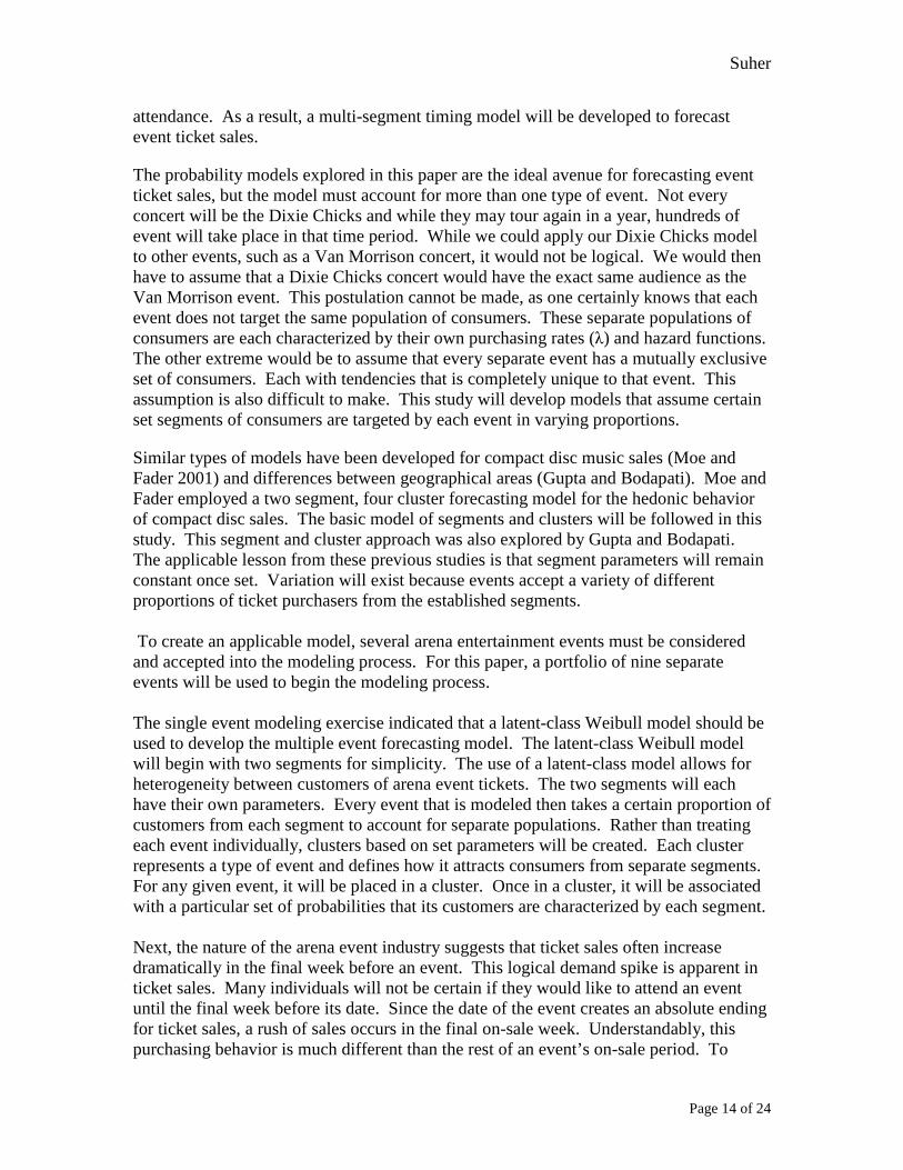
attendance. As a result, a multi-segment timing model will be developed to forecast event ticket sales.

The probability models explored in this paper are the ideal avenue for forecasting event ticket sales, but the model must account for more than one type of event. Not every concert will be the Dixie Chicks and while they may tour again in a year, hundreds of event will take place in that time period. While we could apply our Dixie Chicks model to other events, such as a Van Morrison concert, it would not be logical. We would then have to assume that a Dixie Chicks concert would have the exact same audience as the Van Morrison event. This postulation cannot be made, as one certainly knows that each event does not target the same population of consumers. These separate populations of consumers are each characterized by their own purchasing rates (λ) and hazard functions. The other extreme would be to assume that every separate event has a mutually exclusive set of consumers. Each with tendencies that is completely unique to that event. This assumption is also difficult to make. This study will develop models that assume certain set segments of consumers are targeted by each event in varying proportions.

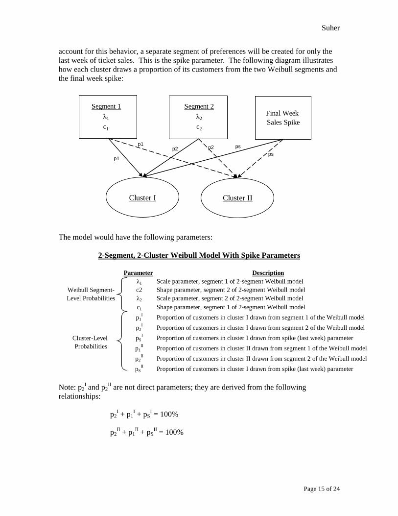
Similar types of models have been developed for compact disc music sales (Moe and Fader 2001) and differences between geographical areas (Gupta and Bodapati). Moe and Fader employed a two segment, four cluster forecasting model for the hedonic behavior of compact disc sales. The basic model of segments and clusters will be followed in this study. This segment and cluster approach was also explored by Gupta and Bodapati. The applicable lesson from these previous studies is that segment parameters will remain constant once set. Variation will exist because events accept a variety of different proportions of ticket purchasers from the established segments. To create an applicable model, several arena entertainment events must be considered and accepted into the modeling process. For this paper, a portfolio of nine separate events will be used to begin the modeling process. The single event modeling exercise indicated that a latent-class Weibull model should be used to develop the multiple event forecasting model. The latent-class Weibull model will begin with two segments for simplicity. The use of a latent-class model allows for heterogeneity between customers of arena event tickets. The two segments will each have their own parameters. Every event that is modeled then takes a certain proportion of customers from each segment to account for separate populations. Rather than treating each event individually, clusters based on set parameters will be created. Each cluster represents a type of event and defines how it attracts consumers from separate segments. For any given event, it will be placed in a cluster. Once in a cluster, it will be associated with a particular set of probabilities that its customers are characterized by each segment. Next, the nature of the arena event industry suggests that ticket sales often increase dramatically in the final week before an event. This logical demand spike is apparent in ticket sales. Many individuals will not be certain if they would like to attend an event until the final week before its date. Since the date of the event creates an absolute ending for ticket sales, a rush of sales occurs in the final on-sale week. Understandably, this purchasing behavior is much different than the rest of an event’s on-sale period. To

Suher

Page 15 of 24

account for this behavior, a separate segment of preferences will be created for only the last week of ticket sales. This is the spike parameter. The following diagram illustrates how each cluster draws a proportion of its customers from the two Weibull segments and the final week spike:

Segment 1 Segment 2 λ1

c1

λ2

c2

Final Week Sales Spike

Cluster I Cluster II

p1

p1p2 psp2

ps

The model would have the following parameters:

2-Segment, 2-Cluster Weibull Model With Spike Parameters

Parameter Descriptionλ1 Scale parameter, segment 1 of 2-segment Weibull modelc2 Shape parameter, segment 2 of 2-segment Weibull modelλ2 Scale parameter, segment 2 of 2-segment Weibull modelc1 Shape parameter, segment 1 of 2-segment Weibull model

p1I Proportion of customers in cluster I drawn from segment 1 of the Weibull model

p2I Proportion of customers in cluster I drawn from segment 2 of the Weibull model

pSI Proportion of customers in cluster I drawn from spike (last week) parameter

p1II Proportion of customers in cluster II drawn from segment 1 of the Weibull model

p2II Proportion of customers in cluster II drawn from segment 2 of the Weibull model

pSII Proportion of customers in cluster I drawn from spike (last week) parameter

Weibull Segment-Level Probabilities

Cluster-Level Probabilities

Note: p2

I and p2II are not direct parameters; they are derived from the following

relationships:

p2I + p1

I + pSI = 100%

p2

II + p1II + pS

II = 100%

Suher

Page 16 of 24

Under these parameters, the cumulative number of tickets sold by week t for an event in a specific cluster is given by:

N x (1-ps) x [(p1 x (1 – e-λ1t^c1)) x (p2 x (1 – e-λ2t^c2))] (t before final week)

N x [ps + (1-ps) x [(p1 x (1 – e-λ1t^c1)) x (p2 x (1 – e-λ2t^c2))]] (final week) Where N is the total number of potential customers by event (see “Additional Data Considerations” above for more on N). Model Estimation The parameters of each segment in the latent-class Weibull model are attained by minimizing the non-linear leased squares error between actual ticket sales and predicted ticket sales across all nine events. Microsoft Excel’s solver function is used for this optimization. Our model uses discrete assignment of events into clusters. The steps of the model estimation are as follows

1. Set up initial clusters: Randomly assign all events into a particular cluster. 2. Optimize each cluster: Use Excel’s solver tool to optimize the parameters for

each cluster using Log Likelihood. This method involved changing the parameters to maximize the sum of Log Likelihood values across all events’ chosen clusters.

3. Reassign clusters: Once cluster parameters are set, move events to the cluster

that has the best fit (lowest sum of squared error).

4. Iterate: Go back to optimizing each cluster. Continue reassigning events to clusters until the parameters are set and each event is in the cluster that provides the best fit.

To prevent possible bias within the solver model, this process is conducted several times with events beginning in different clusters. It did not appear that the initial random assignment of events into clusters affected the ending parameters and event distribution. The resulting clusters were the same regardless of initial event placement. The final model was made with two segments, a final week spike segment, and two clusters. It is illustrated below.

Suher

Page 17 of 24

Final Model Results: 2 Clusters, 2 Segments, 1 Spike for Last Week of Sales

Empirical Analysis The figure above provides the parameter estimates for a model with two segments, one spike for last week of sales, and two clusters. The consumers belonging to the first segment have a low scale parameter (λ=0.39) and a Weibull hazard rate with a declining positive slope. Their natural behavior is that ‘absence makes the heart grow fonder.’ They have a relatively low rate of ticket purchasing tendencies and tend to purchase more tickets over time at a declining rate. The consumers in the second segment have an even lower scale parameter (λ=0.05) and a Weibull hazard rate with a declining positive slope. These consumers are more rapid buyers, eager to purchase tickets before consumers in Segment I. They have a higher rate of purchasing tendency, but have a similar tendency to purchase more tickets at a declining rate over time. The Final Week Sales Spike is a segment that describes a separate set of buying patterns unique to the last week of ticket sales. This segment represents consumers who wait until 7 days or less before the event date to purchase their tickets. The two clusters that have been formed are Cluster I and Cluster II. Cluster I accounts for eight events in the model and Cluster II accounts for five events in the model. Cluster I is predominately (64%) composed of customers in Segment 2. This indicates that events in Cluster I (are subject to customers that tend to purchase more tickets up front and less as the event date nears. The other 36% of consumers in Cluster I are 31% Segment 1 and 6% Final Week Sales Spike. Understandably, some customers do wait until later in the on-sale window to purchase their tickets. Cluster II is predominately composed of customers from Segment 1 (76%). This indicates that events in Cluster II attract customers that purchase more tickets as time progresses. The second cluster is composed of 4% Final Week Sales Spike segment, indicating there is not as strong of a ticket purchasing rush in the final week.

Suher

Page 18 of 24

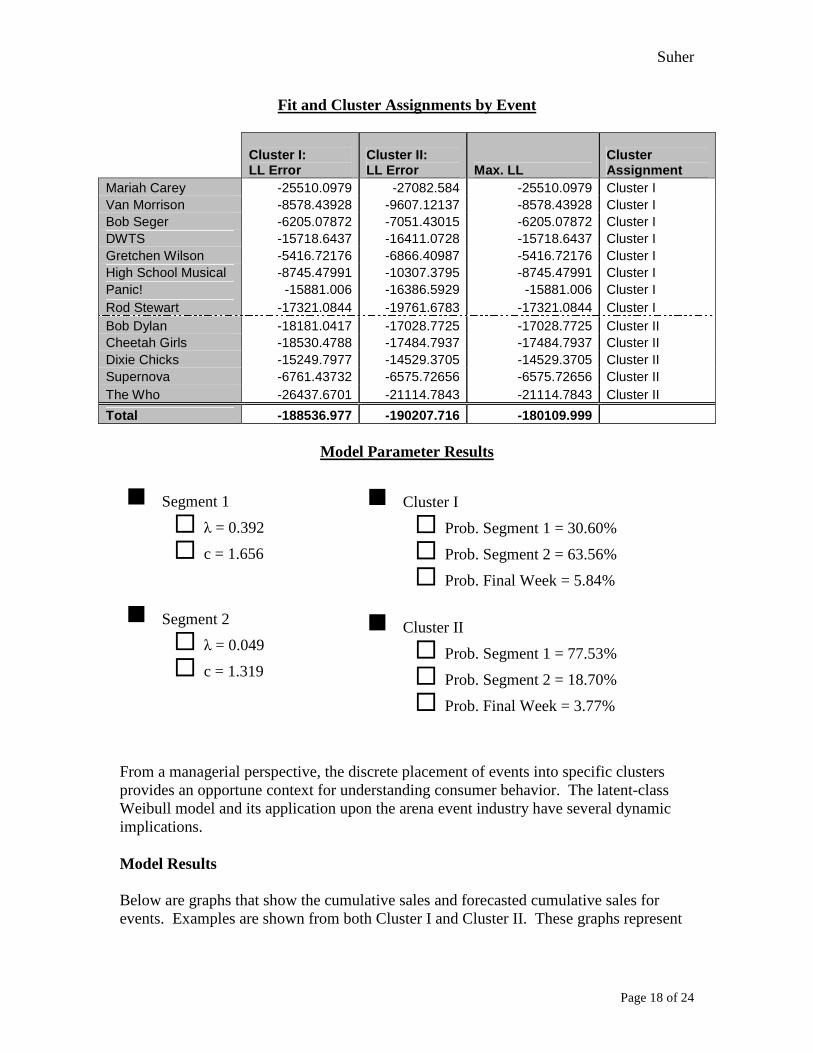
Fit and Cluster Assignments by Event

Cluster I: LL Error

Cluster II: LL Error Max. LL

Cluster Assignment

Mariah Carey -25510.0979 -27082.584 -25510.0979 Cluster I Van Morrison -8578.43928 -9607.12137 -8578.43928 Cluster I Bob Seger -6205.07872 -7051.43015 -6205.07872 Cluster I DWTS -15718.6437 -16411.0728 -15718.6437 Cluster I Gretchen Wilson -5416.72176 -6866.40987 -5416.72176 Cluster I High School Musical -8745.47991 -10307.3795 -8745.47991 Cluster I Panic! -15881.006 -16386.5929 -15881.006 Cluster I Rod Stewart -17321.0844 -19761.6783 -17321.0844 Cluster I Bob Dylan -18181.0417 -17028.7725 -17028.7725 Cluster II Cheetah Girls -18530.4788 -17484.7937 -17484.7937 Cluster II Dixie Chicks -15249.7977 -14529.3705 -14529.3705 Cluster II Supernova -6761.43732 -6575.72656 -6575.72656 Cluster II The Who -26437.6701 -21114.7843 -21114.7843 Cluster II

Total -188536.977 -190207.716 -180109.999

Model Parameter Results

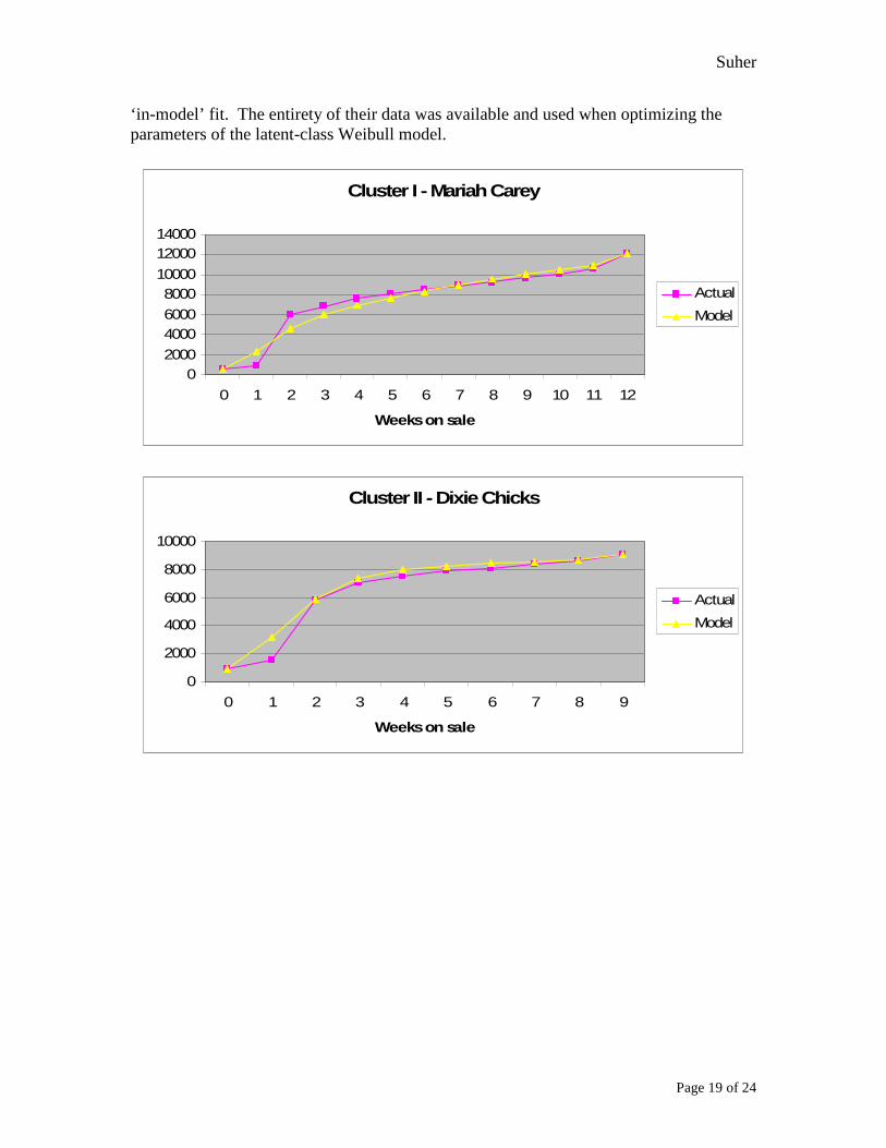
From a managerial perspective, the discrete placement of events into specific clusters provides an opportune context for understanding consumer behavior. The latent-class Weibull model and its application upon the arena event industry have several dynamic implications. Model Results Below are graphs that show the cumulative sales and forecasted cumulative sales for events. Examples are shown from both Cluster I and Cluster II. These graphs represent

� Segment 1

� λ = 0.392

� c = 1.656

� Segment 2

� λ = 0.049

� c = 1.319

� Cluster I

� Prob. Segment 1 = 30.60%

� Prob. Segment 2 = 63.56%

� Prob. Final Week = 5.84%

� Cluster II

� Prob. Segment 1 = 77.53%

� Prob. Segment 2 = 18.70%

� Prob. Final Week = 3.77%

Suher

Page 19 of 24

‘in-model’ fit. The entirety of their data was available and used when optimizing the parameters of the latent-class Weibull model.

Cluster I - Mariah Carey

02000

40006000

800010000

1200014000

0 1 2 3 4 5 6 7 8 9 10 11 12

Weeks on sale

Actual

Model

Cluster II - Dixie Chicks

0

2000

4000

6000

8000

10000

0 1 2 3 4 5 6 7 8 9

Weeks on sale

Actual

Model

Suher

Page 20 of 24

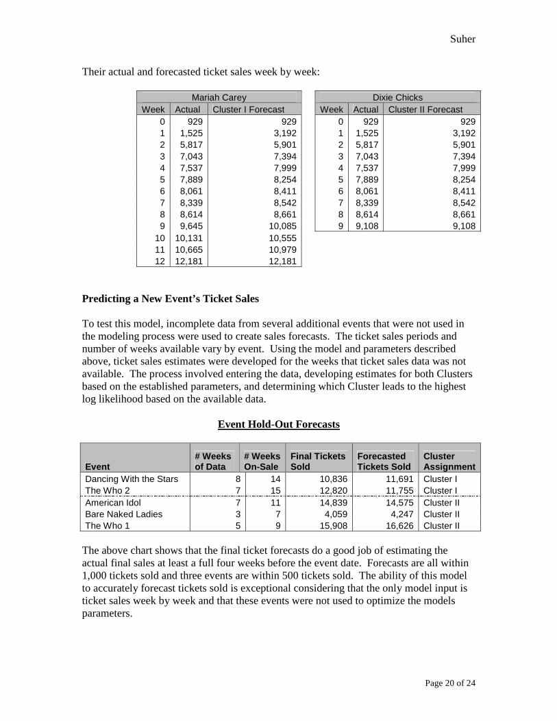
Their actual and forecasted ticket sales week by week:

Mariah Carey Dixie Chicks Week Actual Cluster I Forecast Week Actual Cluster II Forecast

0 929 929 0 929 929 1 1,525 3,192 1 1,525 3,192 2 5,817 5,901 2 5,817 5,901 3 7,043 7,394 3 7,043 7,394 4 7,537 7,999 4 7,537 7,999 5 7,889 8,254 5 7,889 8,254 6 8,061 8,411 6 8,061 8,411 7 8,339 8,542 7 8,339 8,542 8 8,614 8,661 8 8,614 8,661 9 9,645 10,085 9 9,108 9,108

10 10,131 10,555 11 10,665 10,979 12 12,181 12,181

Predicting a New Event’s Ticket Sales To test this model, incomplete data from several additional events that were not used in the modeling process were used to create sales forecasts. The ticket sales periods and number of weeks available vary by event. Using the model and parameters described above, ticket sales estimates were developed for the weeks that ticket sales data was not available. The process involved entering the data, developing estimates for both Clusters based on the established parameters, and determining which Cluster leads to the highest log likelihood based on the available data.

Event Hold-Out Forecasts

Event # Weeks of Data

# Weeks On-Sale

Final Tickets Sold

Forecasted Tickets Sold

Cluster Assignment

Dancing With the Stars 8 14 10,836 11,691 Cluster I The Who 2 7 15 12,820 11,755 Cluster I American Idol 7 11 14,839 14,575 Cluster II Bare Naked Ladies 3 7 4,059 4,247 Cluster II The Who 1 5 9 15,908 16,626 Cluster II

The above chart shows that the final ticket forecasts do a good job of estimating the actual final sales at least a full four weeks before the event date. Forecasts are all within 1,000 tickets sold and three events are within 500 tickets sold. The ability of this model to accurately forecast tickets sold is exceptional considering that the only model input is ticket sales week by week and that these events were not used to optimize the models parameters.

Suher

Page 21 of 24

Below are two events and the plot of their actual cumulative tickets sold and the forecasted tickets sold for both clusters.

Dancing with the Stars

0

20004000

60008000

1000012000

14000

0 1 2 3 4 5 6 7 8 9 10 11 12 13 14

Week

Tic

kets Paid Tix

Cluster I

Cluster II

American Idol

0

5000

10000

15000

20000

0 1 2 3 4 5 6 7 8 9 10 11

Week

Tic

kets Paid Tix

Cluster I

Cluster II

Week-by-Week Forecast Readjustment When a ticket forecast estimate is made, the chosen cluster is determined by the log likelihood values for the available weeks of data. As the number of weeks used to create the forecast change, the model’s log likelihood value will change. It is possible that a single event may change its optimal cluster as additional data is brought into the forecast. Below is a convergence graph to illustrate this pattern.

Suher

Page 22 of 24

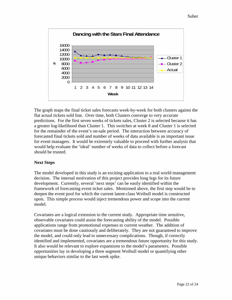
Dancing with the Stars Final Attendance

02000400060008000

10000120001400016000

1 2 3 4 5 6 7 8 9 10 11 12 13 14

Week

#Cluster 1

Cluster 2

Actual

The graph maps the final ticket sales forecasts week-by-week for both clusters against the flat actual tickets sold line. Over time, both Clusters converge to very accurate predictions. For the first seven weeks of tickets sales, Cluster 2 is selected because it has a greater log-likelihood than Cluster 1. This switches at week 8 and Cluster 1 is selected for the remainder of the event’s on-sale period. The interaction between accuracy of forecasted final tickets sold and number of weeks of data available is an important issue for event managers. It would be extremely valuable to proceed with further analysis that would help evaluate the ‘ideal’ number of weeks of data to collect before a forecast should be trusted. Next Steps The model developed in this study is an exciting application to a real world management decision. The internal motivation of this project provides long legs for its future development. Currently, several ‘next steps’ can be easily identified within the framework of forecasting event ticket sales. Mentioned above, the first step would be to deepen the event pool for which the current latent-class Weibull model is constructed upon. This simple process would inject tremendous power and scope into the current model. Covariates are a logical extension to the current study. Appropriate time sensitive, observable covariates could assist the forecasting ability of the model. Possible applications range from promotional expenses to current weather. The addition of covariates must be done cautiously and deliberately. They are not guaranteed to improve the model, and could only lead to unnecessary complications. Though, if correctly identified and implemented, covariates are a tremendous future opportunity for this study. It also would be relevant to explore expansions to the model’s parameters. Possible opportunities lay in developing a three segment Weibull model or quantifying other unique behaviors similar to the last week spike.

Suher

Page 23 of 24

Finally, a turn-key, stand alone software program for managerial decision making is the logical final product. Within the framework of this current study, it is easy to imagine a software program that provides attendance forecasts. A dynamic program could automatically input advanced ticket sales data and output expected attendance as the event date approaches. Further, a model could be developed to continuously update itself and continuously predictions every single day ticket sales data is collected. This software would be an invaluable tool for event managers industry wide. Conclusion and Discussion In this paper, we created a model for forecasting event ticket sales. The value of this predictive model is tremendous. Arena entertainment is saturated with high variable costs that depend upon ultimate attendance values. Improved estimations of final attendance will allow managers to make better decisions as an event approaches. The current model has a large amount of room for development. It must be expanded to include many more events and acknowledge possible covariates. These improvements are easily attainable and fit within this paper’s current framework. The findings in this study show that the pursuit of a probability model to forecast event ticket sales is very promising. With a limited number of events, only thirteen, the patterns and qualities of a precise and powerful model begin to appear. Events were logically placed into clusters and often their predictions were impressively accurate. These small successes provide immense motivation to expand upon the current study. The value of a real application is undeniable. This project is particularly compelling because it is rooted within a tangible industry issue. A ticket forecasting model would be immediately applicable and valuable to the arena entertainment industry.

Suher

Page 24 of 24

References Fader, Peter S. Chapter 4: Modeling Single Event Timing Data. Fader, Peter S. VOD handout – timing models. Gupta, Sahin and Anand V. Bodapati (1999), “Understanding Similarities and

Differences in Consumer Segmentation Across Markets,” working paper, Northwestern University.

Moe, Wendy W., Peter S. Fader. 2001. Modeling hedonic portfolio products: A joint

segmentation analysis of music CD sales. J. Marketing Res. 38 (3) 376-385.