Forecasting European Industrial Production withMultivariate Singular Spectrum Analysis

Anatoly Zhigljavskya∗, Hossein Hassania, and Saeed HeravibaCentre for Optimisation and Its Applications, Cardiff School of Mathematics, CF24 4AG

bCardiff Business School, Cardiff University, CF10 3EU, UK.

Abstract

In recent years the Singular Spectrum Analysis (SSA) technique, used as a pow-erful technique in time series analysis, has been developed and applied to manypractical problems. The aim of this research is to develop theoretical and method-ological aspects of the multivariate SSA (MSSA) technique and to demonstrate thatMSSA can also be considered as a powerful method of time series analysis and fore-casting. We use the UK Industrial Production series to illustrate the main findings.The performance of the SSA technique is assessed by applying it to eight seriesmeasuring the monthly seasonally unadjusted industrial production for the mainsectors of the UK economy. The results are compared with those obtained usingthe ARIMA and VAR models.

We also develop the concept of casual relationship between two time series basedon the SSA techniques. We introduce several criteria which characterize this causal-ity. The criteria are based on the forecasting accuracy and the predictability of thedirection of change. The performance of the proposed tests is examined using thesame data, the UK industrial production series.Keywords: Singular Spectrum Analysis, Forecasting, Causality, The UK industrialproduction series.

1 Introduction

Econometric methods have been widely used to forecast the evolution of quarterly andyearly national account data. However, many of the structural or time series forecastingmodels have failed to accurately predict economic time series. This is due to technologicaladvances, change in government policies and also change in consumer preferences. Theseshocks cause structural changes in these time series making them nonstationary. Develop-ment of a methodology which is robust under these changes is of paramount importancein accurate prediction of macroeconomic time series.

There are several reasons that classical model does not have a good performance formodelling and forecasting economic and financial time series. First, an economic modelthat has been established to have validity in explaining a relationship under one set ofassumptions is useless if the assumptions are not valid. Model assumptions include not

∗E-mail addresses: Zhigljavskyaa@cf.ac.uk, hassanih@cf.ac.uk, Heravis@cf.ac.uk

1

only those that can be expressed as predicates on model parameters but others with morequalitative or asymptotic form (for more information see [1]).

Moreover, many structural econometric and time series models devised for forecastingmacroeconomic time series are based on restrictive assumptions of normality and linearityof the observed data. The methods that do not depend on these assumptions could bevery useful for modelling and forecasting economics data. On the other hand classicalmethods of forecasting such as ARIMA type models are based on the assumption such asstationarity of the series and normality of residuals (see, for example, [2], [3] and referencestherein) .

Additionally, some of the previous research have considered economic and financialtime series as deterministic, linear dynamical systems. In this case, the linear modelscan be used for modelling and forecasting. However, many financial time series exhibitnonlinear behavior (see, for example, [4, 5, 6, 7]); and therefore, we should use nonlinearmethods. In addition a method that works well for both linear and nonlinear, station-ary and non stationary time series is ideal for modelling and forecasting the real timeseries data. The Singular Spectrum Analysis (SSA) in a technique that is free from allthese assumptions. The SSA technique is a nonparametric technique of time series anal-ysis incorporating the elements of classical time series analysis, multivariate statistics,multivariate geometry, dynamical systems and signal processing[8]. Note also that SSAnaturally incorporates the filtering of the series and the SVD.

The basic SSA method consists of two complementary stages: decomposition andreconstruction; both stages include two separate steps. At the first stage we decompose theseries and at the second stage we reconstruct the original series and use the reconstructedseries for forecasting new data points. The main concept in studying the properties ofSSA is ‘separability’, which characterizes how well different components can be separatedfrom each other. The absence of approximate separability is often observed in series withcomplex structure. For these series and series with special structure, there are differentways of modifying SSA leading to different versions such as SSA with single and doublecentering, Toeplitz SSA, and sequential SSA [8].

It is worth noting that although some probabilistic and statistical concepts are em-ployed in the SSA-based methods, we do not have to make any statistical assumptionssuch as stationarity of the series or normality of the residuals. SSA is a very useful toolwhich can be used for solving the following problems:

finding trends of different resolution;smoothing;extraction of seasonality components;simultaneous extraction of cycles with small and large periods;extraction of periodicities with varying amplitudes;simultaneous extraction of complex trends and periodicities;finding structure in short time series.

Solving all these problems correspond to the so-called basic capabilities of SSA. Inaddition, the method has several essential extensions. First, the multivariate version ofthe method permits the simultaneous expansion of several time series; see, for example[10]. Second, the SSA ideas lead to several forecasting procedures for time series; see[8, 10]. Also, the same ideas are used in [8] and [14] for change-point detection in timeseries. For comparison with classical methods, ARIMA, ARAR algorithm and Holt-

2

Winter, see [15] and [16], and for comparison between multivariate SSA and VAR modelsee [17]. For automatic methods of identification within the SSA framework see [18] andfor recent work in ‘Caterpillar’-SSA software as well as new developments see [19]. Afamily of causality tests based on the SSA technique has also been considered in [20].

In the area of nonlinear time series analysis SSA was considered as a technique thatcould compete with more standard methods. There are a number of research that con-sidered SSA as a filtering method in (see, for example, [21] and references therein). Inanother research, the noise information extracted using the SSA technique, has been usedas a biomedical diagnostic test [22]. The SSA technique also used as a filtering methodfor longitudinal measurements. It has been shown that noise reduction is important forcurve fitting in growth curve models, and that SSA can be employed as a powerful toolfor noise reduction for longitudinal measurements [23].

The monthly industrial production indices for the UK, have been previously analysedin linear and nonlinear contexts in [16], [24] and [25]. The eight series examined for theUK, are interesting and important since they ranging from traditional industrial sections(Basic metals) to Food and Electricity and Gas. These eight time series contribute for atleast 50% to the aggregate industrial production in the UK economics.

Osborn et al. [24] have considered the extent and nature of seasonality in these series.Seasonality accounts for at least 80% of variation in all series (except vehicles) in theUK. In our recent research [16], we used Singular Spectrum Analysis (SSA), ARIMA andHolt-Winter methods for forecasting seasonally unadjusted monthly data on industrialproduction indicators in Germany, France and the UK. We have demonstrated that SSAis a very powerful tool for analyzing and predicting these series. The SSA techniquedecomposes the original time series into a sum of small number of independent and in-terpretable components such as slowly varying trend, oscillatory components and noise.Theoretical and practical foundations of the SSA technique can be found in [8].

Hassani et al. [16] showed that the quality of 1-step ahead forecasts are similar forARIMA and SSA; Holt-Winter forecasts being slightly worse. The quality of SSA forecastsat horizons h = 3, 6 and 12 is much better than the quality of ARIMA and Holt-Winterforecasts. As h increases, the quality of ARIMA and Holt-Winter forecasts becomes worse.Also the standard deviation of the ARIMA and Holt-Winter forecasts increases almostlinearly with h. The situation is totally different for the SSA forecasts: the quality ofSSA forecasts is almost independent of the value of h (for the values of h considered inour research).

Another important aspect of the SSA (which can be very useful in economics) is that,unlike many other methods, it works well even for small sample size (see, for example,[12] and [15]). We found that SSA works well for small sample sizes, as for the UK withthe sample size of 84 observations [16].

Hassani et al. [16] also showed that three methods perform similarly well in predictingthe direction of change for small h. However, SSA outperforms the Holt-Winter andARIMA models at longer horizons and hence can be considered as a reliable method forpredicting recessions and expansions.

The present project aims to predict the monthly industrial production indices for theUK using multivariate singular spectrum analysis (MSSA). Here we develop the method-ology of forecasting these series based on MSSA. Preliminary results indicate that theSSA can further improve the results of univariate SSA for the these series. The quality ofMSSA forecasts can be higher when the analysed series are interdependent and therefore

3

highly correlated. We also use MSSA to investigate the causality among these series. Asthese series are non-stationary and non-linear, we use nonlinear correlation which is basedon the Mutual information introduced in [26] and [27], and has also been used in [21].

We are motivated to use SSA because of its capability in dealing with non-stationaryseries. Given that the dynamics of some industrial production series has gone throughstructural changes during the time period under consideration, one needs to make sure thatthe method of prediction is not sensitive to the dynamical changes. Moreover, contrary tothe traditional methods of time series forecasting (both autoregressive or structural modelsthat assume normality and stationarity of the series), SSA method is non-parametric andmakes no prior assumptions about the data. The data considered in this study hasa complex structure of this kind; as a consequence, we found superiority of SSA overclassical techniques. Additionally, SSA method decomposes a series into its componentparts, and reconstruct the series without including the random (noise) component.

The structure of this report is as follows. A brief introduction of the SSA methodis represented in Section 2. The descriptive statistics of the series and the results ofvarious tests (such as normality, nonlinearity, stationarity) are presented in Section 3.The performance of ARIMA, SSA, MSSA and VAR is considered in Section 4. A newcasuality test based on the SSA technique is introduced in Section 5. Finally, Section 6presents a summary of the study and some concluding remarks.

2 Singular Spectrum Analysis

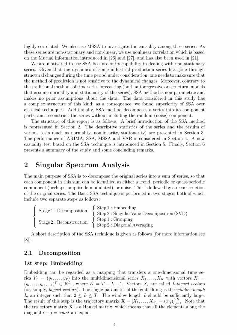
The main purpose of SSA is to decompose the original series into a sum of series, so thateach component in this sum can be identified as either a trend, periodic or quasi-periodiccomponent (perhaps, amplitude-modulated), or noise. This is followed by a reconstructionof the original series. The Basic SSA technique is performed in two stages, both of whichinclude two separate steps as follows:

Stage 1 : Decomposition

{Step 1 : EmbeddingStep 2 : Singular Value Decomposition (SVD)

Stage 2 : Reconstruction

{Step 1 : GroupingStep 2 : Diagonal Averaging

A short description of the SSA technique is given as follows (for more information see[8]).

2.1 Decomposition

1st step: Embedding

Embedding can be regarded as a mapping that transfers a one-dimensional time se-ries YT = (y1, . . . , yT ) into the multidimensional series X1, . . . , XK with vectors Xi =(yi, . . . , yi+L−1)

T ∈ RL , where K = T − L +1. Vectors Xi are called L-lagged vectors(or, simply, lagged vectors). The single parameter of the embedding is the window lengthL, an integer such that 2 ≤ L ≤ T . The window length L should be sufficiently large.The result of this step is the trajectory matrix X = [X1, . . . , XK ] = (xij)

L,Ki,j=1. Note that

the trajectory matrix X is a Hankel matrix, which means that all the elements along thediagonal i + j = const are equal.

4

2nd step: Singular Value Decomposition (SVD)

The second step, the SVD step, makes the singular value decomposition of the trajectorymatrix and represents it as a sum of rank-one bi-orthogonal elementary matrices. Denoteby λ1, . . . , λL the eigenvalues of XXT in decreasing order of magnitude (λ1 ≥ . . . λL ≥ 0)and by U1, . . . , UL the orthonormal system of the eigenvectors of the matrix XXT corre-sponding to these eigenvalues. Set

d = max(i, such that λi > 0) = rank X.

If we denote Vi = XT Ui/√

λi, then the SVD of the trajectory matrix can be written as:

X = X1 + · · ·+ Xd, (1)

where Xi =√

λiUiViT .

SVD (1) is optimal in the sense that among all the matrices X(r) of rank r < d,the matrix

∑ri=1 Xi provides the best approximation to the trajectory matrix X, so that

‖ X− X(r) ‖ is minimum. Here the norm of a matrix Y is defined as√〈Y,Y〉, where the

scalar product of two matrices Y = (yij)q,si,j=1 and Z = (zij)

q,si,j=1 is 〈Y,Z〉 =

∑q,si,j=1 yijzij.

Note that ‖ X ‖2 =∑d

i=1 λi and ‖ Xi ‖2 = λi for i = 1, . . . , d. Thus, we can consider the

ratio λi/∑d

i=1 λi as the characteristic of the contribution of the matrix Xi to expansion

(1). Consequently,∑r

i=1 λi/∑d

i=1 λi, the sum of the first r ratios, is the characteristic ofthe optimal approximation of the trajectory matrix by the matrices of rank r .

2.2 Reconstruction

1st Step: Grouping

The grouping step corresponds to splitting the elementary matrices into several groupsand summing the matrices within each group. Let I = {i1, . . . , ip} be a group of indicesi1, . . . , ip. Then the matrix XI corresponding to the group I is defined as XI = Xi1 +· · · + Xip . The spilt of the set of indices J = {1, . . . , d} into disjoint subsets I1, . . . , Im

corresponds to the representation

X = XI1 + · · ·+ XIm . (2)

The procedure of choosing the sets I1, . . . , Im is called the eigentriple grouping. For agiven group I the contribution of the component XI in the expansion (2) is measured bythe share of the corresponding eigenvalues:

∑i∈I λi/

∑di=1 λi.

2nd Step: Diagonal averaging

The purpose of diagonal averaging is to transform a matrix to the form of a Hankel matrixwhich can be subsequently converted to a time series. If zij stands for an element of amatrix Z, then the k -th term of the resulting series is obtained by averaging zij over alli, j such that i + j = k + 1. This procedure is called diagonal averaging, or Hankelizationof the matrix Z. The result of the Hankelization of a matrix Z is the Hankel matrix HZ.Note that the Hankelization is an optimal procedure in the sense that the matrix HZ

5

is the nearest to Z (with respect to the matrix norm) among all Hankel matrices of thecorresponding size (see [8], Sect. 6.2). In its turn, the Hankel matrix HZ uniquely definesthe series by relating the value in the diagonals to the values in the series.

By applying the Hankelization procedure to all matrix components of (2), we obtain

another expansion X = XI1 + . . . + XIm , where XI1 = HX. This is equivalent to the

decomposition of the initial series YT = (y1, . . . , yT ) into a sum of m series; yt =∑m

k=1 y(k)t ,

where Y(k)T = (y

(k)1 , . . . , y

(k)T ) corresponds to the matrix XIk

. A sensible grouping leads tothe decomposition (1) where the resultant matrices XIk

are almost Hankel ones.

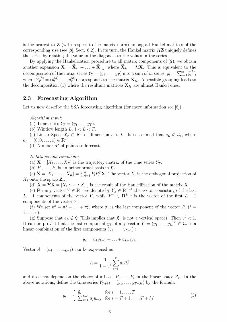
2.3 Forecasting Algorithm

Let us now describe the SSA forecasting algorithm (for more information see [8]):

Algorithm input:(a) Time series YT = (y1, . . . , yT ).(b) Window length L, 1 < L < T .(c) Linear Space Lr ⊂ RL of dimension r < L. It is assumed that eL /∈ Lr, where

eL = (0, 0, . . . , 1) ∈ RL.(d) Number M of points to forecast.

Notations and comments:(a) X = [X1, . . . , XK ] is the trajectory matrix of the time series YT .(b) P1, . . . , Pr is an orthonormal basis in Lr.

(c) X = [X1 : . . . : XK ] =∑r

i=1 PiPTi X. The vector Xi is the orthogonal projection of

Xi onto the space Lr.(d) X = HX = [X1 : . . . : XK ] is the result of the Hankellization of the matrix X.(e) For any vector Y ∈ RL we denote by YM ∈ RL−1 the vector consisting of the last

L − 1 components of the vector Y , while Y O ∈ RL−1 is the vector of the first L − 1components of the vector Y .

(f) We set v2 = π21 + . . . + π2

r , where πi is the last component of the vector Pi (i =1, . . . , r).

(g) Suppose that eL /∈ Lr(This implies that Lr is not a vertical space). Then v2 < 1.It can be proved that the last component yL of any vector Y = (y1, . . . , yL)T ∈ Lr is alinear combination of the first components (y1, . . . , yL−1) :

yL = a1yL−1 + . . . + aL−1y1.

Vector A = (a1, . . . , aL−1) can be expressed as

A =1

1− v2

r∑i=1

πiPOi

and dose not depend on the choice of a basis P1, . . . , Pr in the linear space Lr. In theabove notations, define the time series YT+M = (y1, . . . , yT+M) by the formula

yi =

{yi for i = 1, . . . , T∑L−1

j=1 ajyi−j for i = T + 1, . . . , T + M(3)

6

The numbers yT+1, . . . , yT+M from the M terms of the SSA recurrent forecast. Let usdefine the linear operator P(r) : Lr 7→ RL by the formula

P(r)Y =

(YM

AT YM

), Y ∈ Lr

If setting

Zi =

{Xi for i = 1, . . . , KP(r)Zi−1 for i = K + 1, . . . , K + M

(4)

the matrix Z = [Z1, . . . , ZK+M ] is the trajectory matrix of the series YT+M . Therefore,(4) can be regard as the vector form of (3).

2.4 Multivariate singular spectrum analysis (MSSA)

The use of multivariate singular spectrum analysis (MSSA) for multivariate time serieswas proposed theoretically in the context of nonlinear dynamics in [9]. There are numerousexamples of successful application of the multivariate SSA (see, for example, [1] and [10]).Multivariate (or multichannel) SSA is an extension of the standard SSA to the case ofmultivariate time series. We give a short description of MSSA method as follows.

Assume that we have an M -variate time series yj =(y

(1)j , . . . , y

(M)j

), where j = 1, . . . , T

and let L be window length. Similar to univariate version, we can define the trajectorymatrices X(i) (i=1, . . . , M) of the one-dimensional time series {y(i)

j } (i = 1, . . . ,M). Thetrajectory matrix X can then be defined as

X =

X(1)

...X(M)

. (5)

3 Descriptive Analysis

In this section, we consider descriptive statistics of the 8 series measuring the monthlyseasonally unadjusted industrial production for important sectors of the UK economies.

3.1 The data

The data in this study are taken from Eurostat, the office for National statistics andrepresents eight major components of industrial production in the UK. The two digitcategory industrials examined in this research are seasonally unadjusted monthly indicesfor real output in Food Products, Chemicals, Basic Metals, Fabricated Metals, Machinery,Electrical Machinery, Vehicles and Electricity and Gas industries. The two-digit categoriesexamined in this research are as foloows:

The same 8 series, ending in 1995, have been previously analysed in [24], [25] andending in 2007 in [16]. As explained in these papers, these industries have been chosenprimarily because of their importance and that are the basis of the contribution to totalindustrial production. Here we have updated the data and in all cases the sample periodstarts from January 1978 and ends in July 2009, giving a long series of 380 observations.In line with the usual convention for economic time series and for comparability, all time

7

Short name DetailFood product Manufacture of food products and beverages

Chemicals Manufacture of chemicals and chemical productBasic metals Manufacture of basic metals

Fabricated metal Manufacture of fabricated metal productsMachinery Manufacture of machinery and equipment N.E.C.

Electrical machinery Manufacture of electrical machinery and apparatus N.E.C.Vehicles Manufacture of motor vehicles, trailers and semi-trailers

Electricity and gas Electricity, gas and water supply

Table 1: Industrial production series.

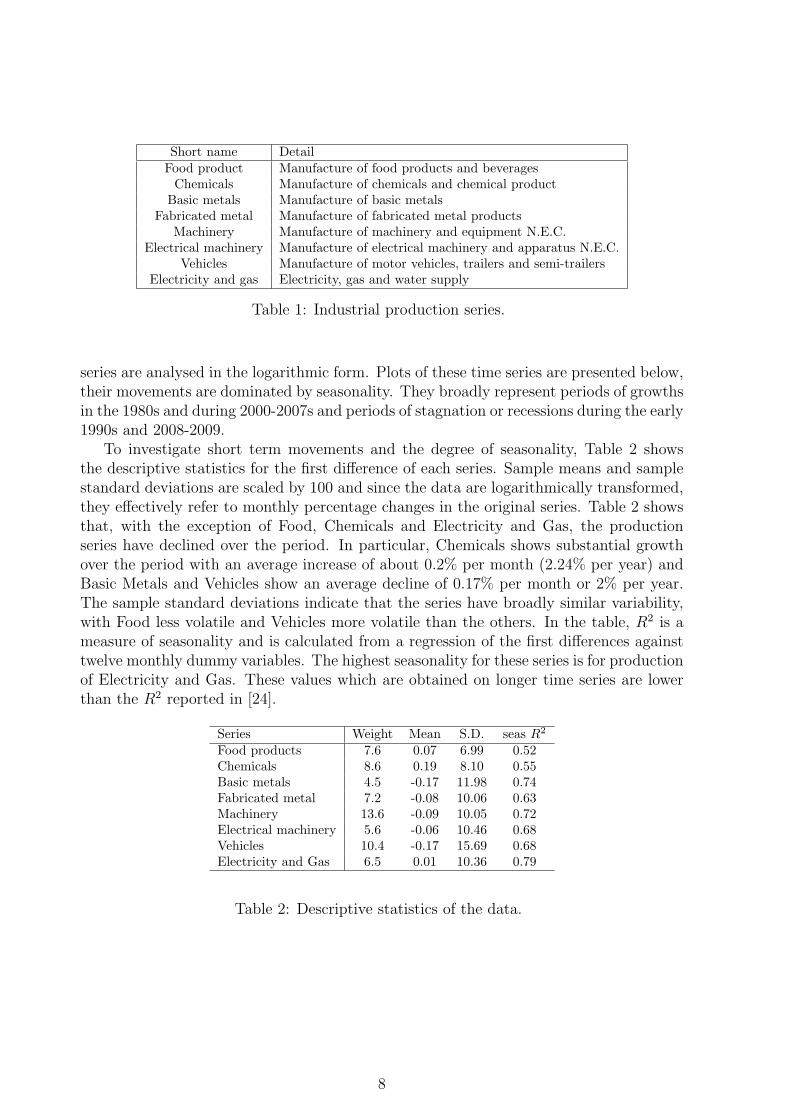
series are analysed in the logarithmic form. Plots of these time series are presented below,their movements are dominated by seasonality. They broadly represent periods of growthsin the 1980s and during 2000-2007s and periods of stagnation or recessions during the early1990s and 2008-2009.

To investigate short term movements and the degree of seasonality, Table 2 showsthe descriptive statistics for the first difference of each series. Sample means and samplestandard deviations are scaled by 100 and since the data are logarithmically transformed,they effectively refer to monthly percentage changes in the original series. Table 2 showsthat, with the exception of Food, Chemicals and Electricity and Gas, the productionseries have declined over the period. In particular, Chemicals shows substantial growthover the period with an average increase of about 0.2% per month (2.24% per year) andBasic Metals and Vehicles show an average decline of 0.17% per month or 2% per year.The sample standard deviations indicate that the series have broadly similar variability,with Food less volatile and Vehicles more volatile than the others. In the table, R2 is ameasure of seasonality and is calculated from a regression of the first differences againsttwelve monthly dummy variables. The highest seasonality for these series is for productionof Electricity and Gas. These values which are obtained on longer time series are lowerthan the R2 reported in [24].

Series Weight Mean S.D. seas R2

Food products 7.6 0.07 6.99 0.52Chemicals 8.6 0.19 8.10 0.55Basic metals 4.5 -0.17 11.98 0.74Fabricated metal 7.2 -0.08 10.06 0.63Machinery 13.6 -0.09 10.05 0.72Electrical machinery 5.6 -0.06 10.46 0.68Vehicles 10.4 -0.17 15.69 0.68Electricity and Gas 6.5 0.01 10.36 0.79

Table 2: Descriptive statistics of the data.

8

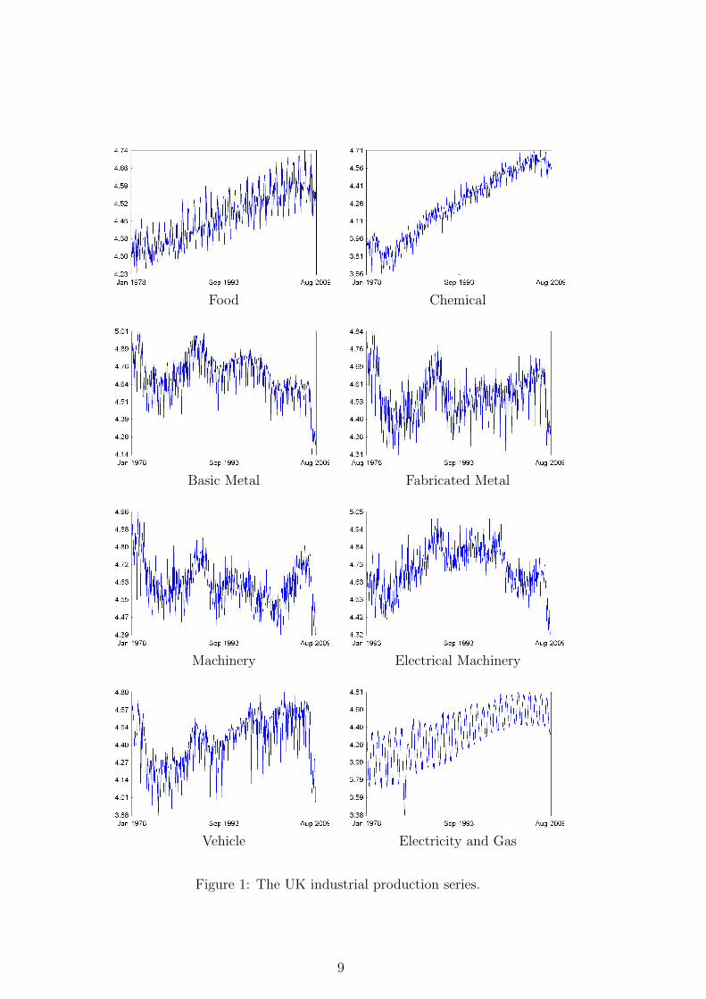
Food Chemical

Basic Metal Fabricated Metal

Machinery Electrical Machinery

Vehicle Electricity and Gas

Figure 1: The UK industrial production series.

9

3.2 Normality Tests

Univariate Normality test

The Anderson-Darling (A-D), Ryan-Joiner (R-J), and Kolmogorov-Smirnov (K-S) testsare used to test if a sample of data came from a population with a specific distribution.The A-D and K-S tests are based on the empirical distribution function and the R-J(similar to Shapiro-Wilk) is based on regression and correlation [28].

All three tests tend to work well in identifying a distribution as not normal when thedistribution under consideration is skewed. All three tests are less discriminating whenthe underlying distribution is a t-distribution and non-normality is due to kurtosis. Ingeneral, among the tests based on the empirical distribution function, the A-D tends tobe more effective in detecting departures in the tails of the distribution. In practice, ifdeparture from normality at the tails is the major concern, many statisticians would usethe A-D test as the first choice. Here we use all the above mentioned tests in order tohave a comprehensive view of non-normality test results for the series.

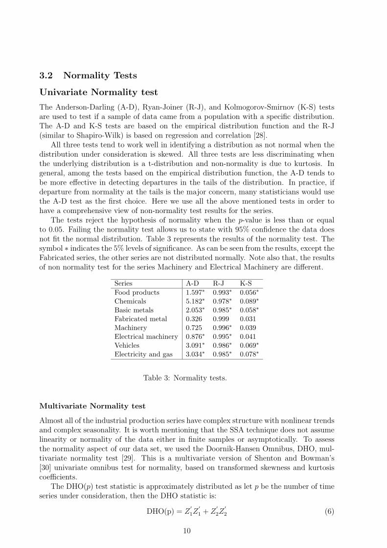
The tests reject the hypothesis of normality when the p-value is less than or equalto 0.05. Failing the normality test allows us to state with 95% confidence the data doesnot fit the normal distribution. Table 3 represents the results of the normality test. Thesymbol ∗ indicates the 5% levels of significance. As can be seen from the results, except theFabricated series, the other series are not distributed normally. Note also that, the resultsof non normality test for the series Machinery and Electrical Machinery are different.

Series A-D R-J K-SFood products 1.597∗ 0.993∗ 0.056∗

Chemicals 5.182∗ 0.978∗ 0.089∗

Basic metals 2.053∗ 0.985∗ 0.058∗

Fabricated metal 0.326 0.999 0.031Machinery 0.725 0.996∗ 0.039Electrical machinery 0.876∗ 0.995∗ 0.041Vehicles 3.091∗ 0.986∗ 0.069∗

Electricity and gas 3.034∗ 0.985∗ 0.078∗

Table 3: Normality tests.

Multivariate Normality test

Almost all of the industrial production series have complex structure with nonlinear trendsand complex seasonality. It is worth mentioning that the SSA technique does not assumelinearity or normality of the data either in finite samples or asymptotically. To assessthe normality aspect of our data set, we used the Doornik-Hansen Omnibus, DHO, mul-tivariate normality test [29]. This is a multivariate version of Shenton and Bowman’s[30] univariate omnibus test for normality, based on transformed skewness and kurtosiscoefficients.

The DHO(p) test statistic is approximately distributed as let p be the number of timeseries under consideration, then the DHO statistic is:

DHO(p) = Z′1Z

′1 + Z

′2Z

′2 (6)

10

where Z′1 = (z11 , . . . , z1p) and Z

′2 = (z21 , . . . , z2p); z1i

is a transformation of the standardunivariate skewness coefficient

√b1, applied to the i-th series, due to D’Agostino [28], and

z2iis a transformation of the standard kurtosis coefficient

√b2, from a gamma distribution

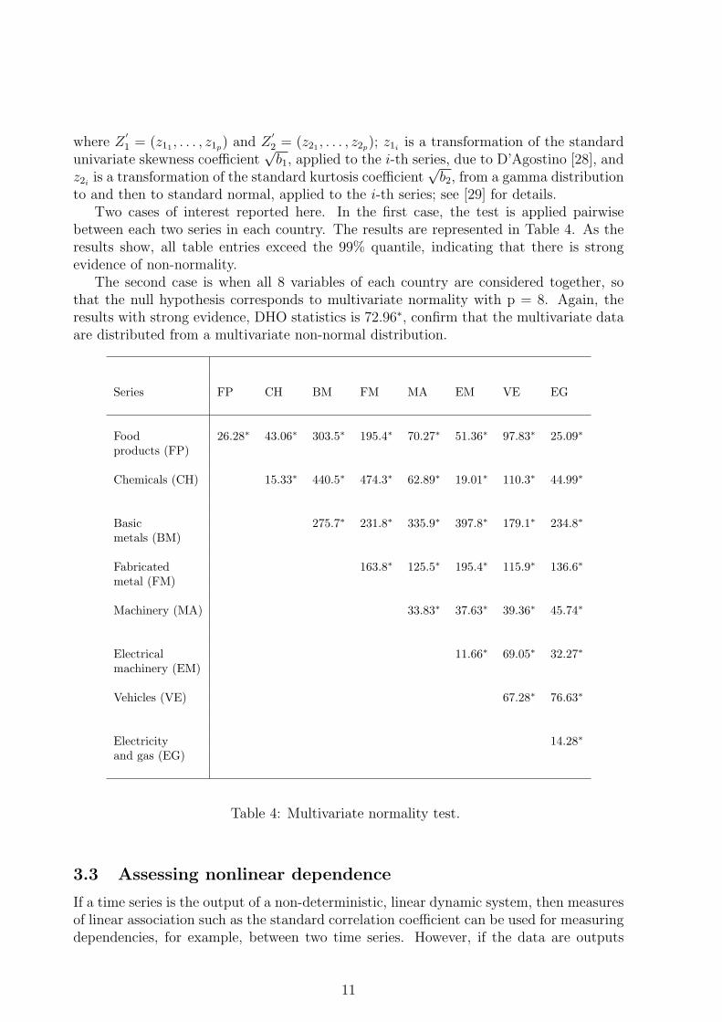
to and then to standard normal, applied to the i-th series; see [29] for details.Two cases of interest reported here. In the first case, the test is applied pairwise

between each two series in each country. The results are represented in Table 4. As theresults show, all table entries exceed the 99% quantile, indicating that there is strongevidence of non-normality.

The second case is when all 8 variables of each country are considered together, sothat the null hypothesis corresponds to multivariate normality with p = 8. Again, theresults with strong evidence, DHO statistics is 72.96∗, confirm that the multivariate dataare distributed from a multivariate non-normal distribution.

Series FP CH BM FM MA EM VE EG

Food 26.28∗ 43.06∗ 303.5∗ 195.4∗ 70.27∗ 51.36∗ 97.83∗ 25.09∗

products (FP)

Chemicals (CH) 15.33∗ 440.5∗ 474.3∗ 62.89∗ 19.01∗ 110.3∗ 44.99∗

Basic 275.7∗ 231.8∗ 335.9∗ 397.8∗ 179.1∗ 234.8∗

metals (BM)

Fabricated 163.8∗ 125.5∗ 195.4∗ 115.9∗ 136.6∗

metal (FM)

Machinery (MA) 33.83∗ 37.63∗ 39.36∗ 45.74∗

Electrical 11.66∗ 69.05∗ 32.27∗

machinery (EM)

Vehicles (VE) 67.28∗ 76.63∗

Electricity 14.28∗

and gas (EG)

Table 4: Multivariate normality test.

3.3 Assessing nonlinear dependence

If a time series is the output of a non-deterministic, linear dynamic system, then measuresof linear association such as the standard correlation coefficient can be used for measuringdependencies, for example, between two time series. However, if the data are outputs

11

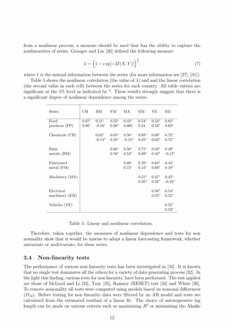
from a nonlinear process, a measure should be used that has the ability to capture thenonlinearities of series. Granger and Lin [26] defined the following measure

λ =(1− exp[−2I(X, Y )]

) 12. (7)

where I is the mutual information between the series (for more information see [27], [31]).Table 5 shows the nonlinear correlation (the value of λ) and and the linear correlation

(the second value in each cell) between the series for each country. All table entries aresignificant at the 5% level as indicated by *. These results strongly suggest that there isa significant degree of nonlinear dependence among the series.

Series CH BM FM MA EM VE EG

Food 0.87∗ 0.51∗ 0.55∗ 0.42∗ 0.54∗ 0.53∗ 0.65∗

products (FP) 0.86∗ -0.16∗ 0.26∗ 0.005 0.24 0.53∗ 0.63∗

Chemicals (CH) 0.62∗ 0.65∗ 0.56∗ 0.69∗ 0.68∗ 0.72∗

-0.14∗ 0.28∗ -0.14∗ 0.25∗ 0.63∗ 0.72∗

Basic 0.66∗ 0.56∗ 0.71∗ 0.62∗ 0.49∗

metals (BM) 0.58∗ 0.53∗ 0.69∗ 0.42∗ -0.12∗

Fabricated 0.66∗ 0.76∗ 0.64∗ 0.44∗

metal (FM) 0.73∗ 0.44∗ 0.69∗ 0.10∗

Machinery (MA) 0.51∗ 0.47∗ 0.45∗

0.35∗ 0.32∗ -0.16∗

Electrical 0.56∗ 0.54∗

machinery (EM) 0.55∗ 0.52∗

Vehicles (VE) 0.55∗

0.53∗

Table 5: Linear and nonlinear correlation.

Therefore, taken together, the measures of nonlinear dependence and tests for nonnormality show that it would be unwise to adopt a linear forecasting framework, whetherunivariate or multivariate, for these series.

3.4 Non-linearity tests

The performance of various non-linearity tests has been investigated in [32]. It is knownthat no single test dominates all the others for a variety of data generating process [32]. Inthe light this finding, various tests for non linearity, have been performed. The test appliedare those of McLeod and Li [33], Tsay [35], Ramsey (RESET) test [34] and White [36].To remove seasonality all tests were computed using models based on seasonal differences(D12). Before testing for non linearity data were filtered by an AR model and tests arecalculated from the estimated residual of a linear fit. The choice of antoregressive laglength can be made on various criteria such as maximising R2 or minimising the Akaike

12

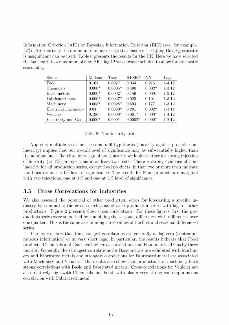
Information Criterion (AIC) or Bayesian Information Criterion (BIC) (see, for example,[37]). Alternatively the minimum number of lags that ensures the Ljung Box, Q, statisticis insignificant can be used. Table 6 presents the results for the UK. Here we have selectedthe lag length to a maximum of 6 by BIC; lag 12 was always included to allow for stochasticseasonality.

Series McLeod Tsay RESET NN LagsFood 0.163 0.007* 0.034 0.215 1-4,12Chemicals 0.000* 0.0005* 0.490 0.002* 1-3,12Basic metals 0.000* 0.0002* 0.156 0.0001* 1-3,12Fabricated metal 0.000* 0.0027* 0.025 0.104 1-3,12Machinery 0.008* 0.0028* 0.693 0.177 1-3,12Electrical machinery 0.04 0.0030* 0.281 0.002* 1-3,12Vehicles 0.196 0.0000* 0.001* 0.000* 1-4,12Electricity and Gas 0.000* 0.000* 0.0002* 0.000* 1-2,12

Table 6: Nonlinearity tests.

Applying multiple tests for the same null hypothesis (linearity against possible non-linearity) implies that our overall level of significance may be substantially higher thanthe nominal one. Therefore for a sign of non-linearity we look at either for strong rejectionof linearity (at 1%) or rejections in at least two tests. There is strong evidence of non-linearity for all production series, except food products, in that two or more tests indicatenon-linearity at the 1% level of significance. The results for Food products are marginalwith two rejections, one at 1% and one at 5% level of significance.

3.5 Cross Correlations for industries

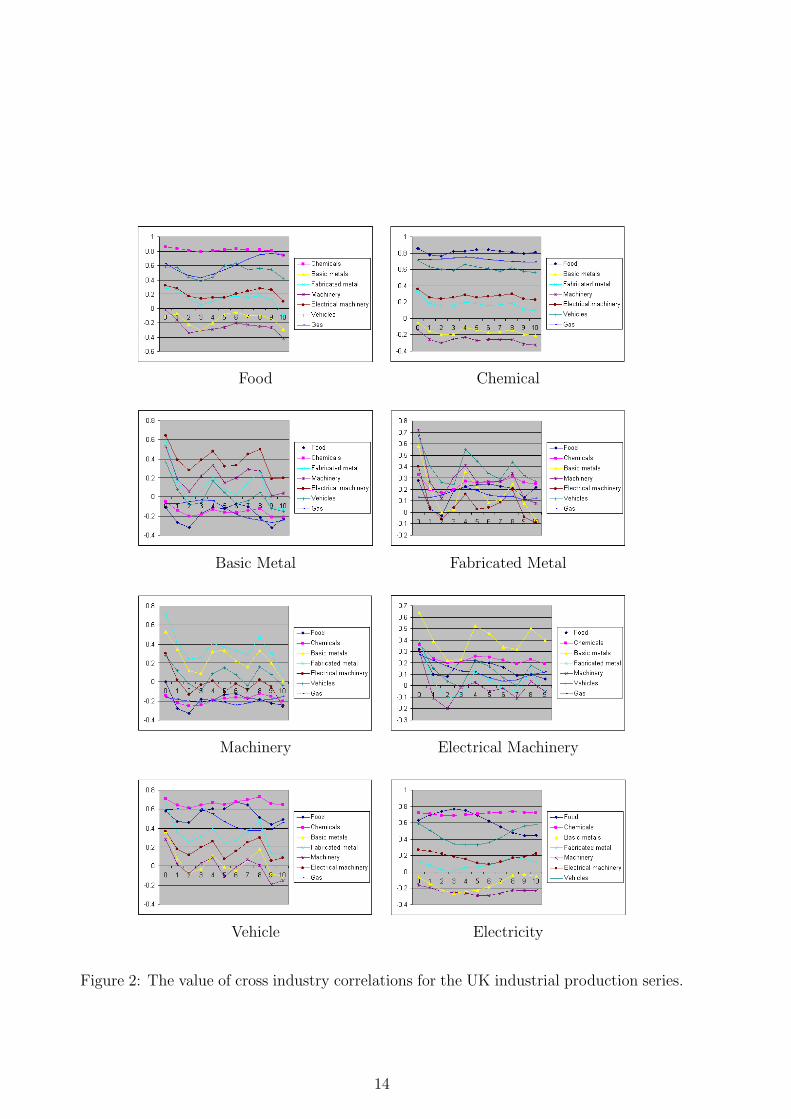
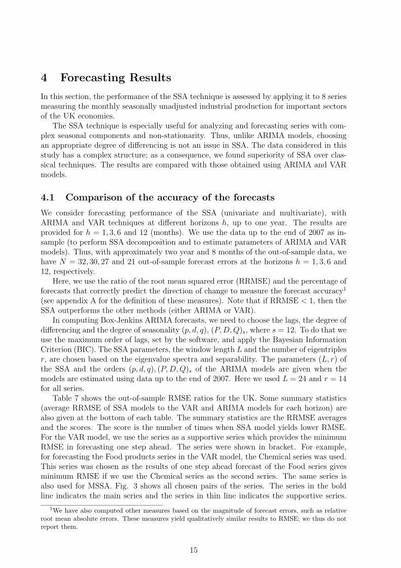
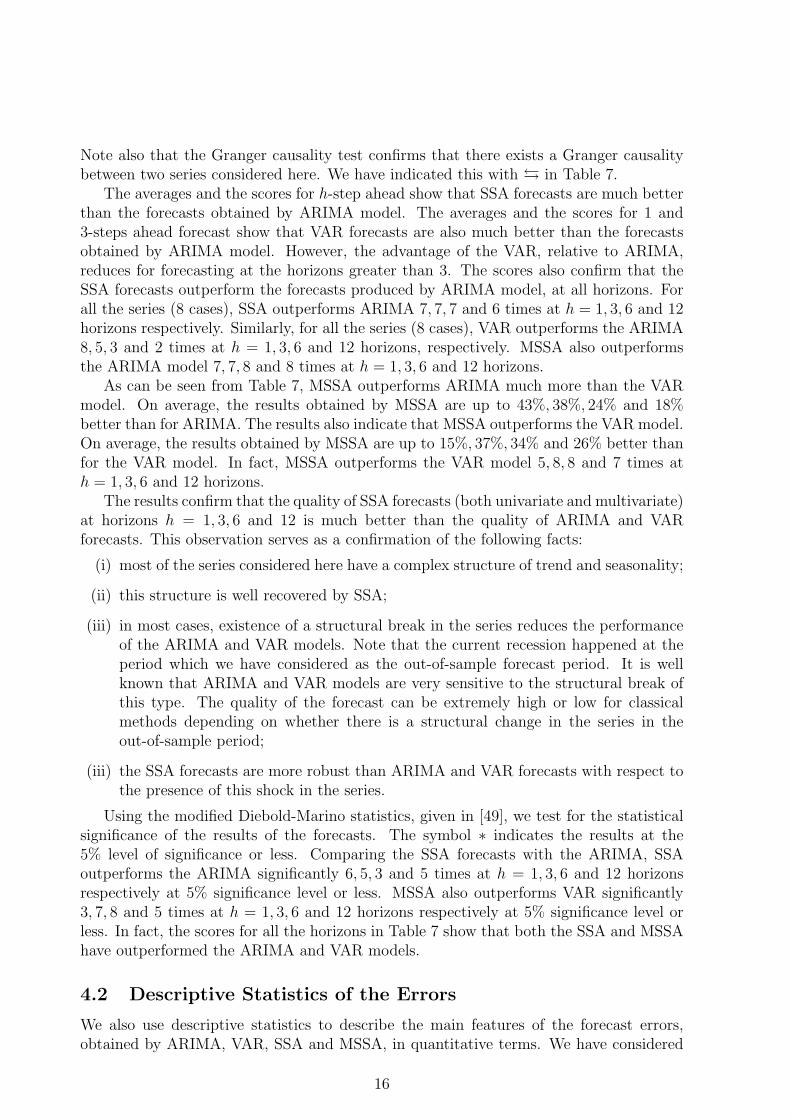
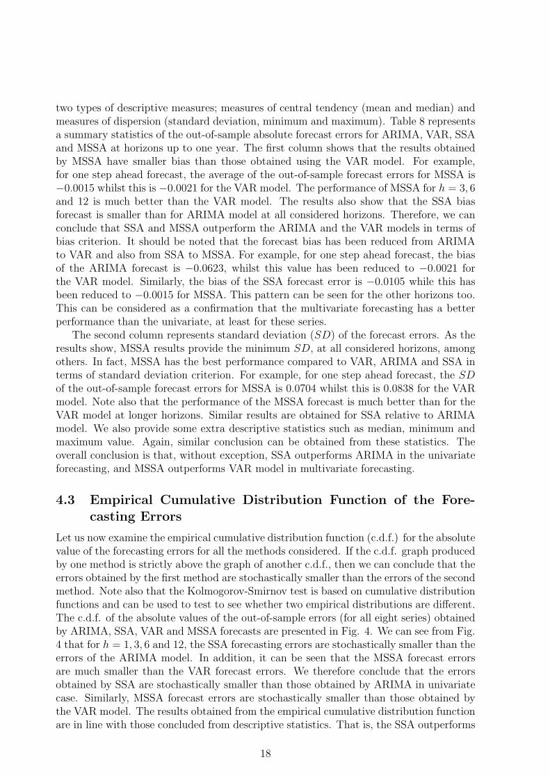
We also assessed the potential of other production series for forecasting a specific in-dustry by computing the cross correlations of each production series with lags of otherproductions. Figure 2 presents these cross correlations. For these figures, first the pro-ductions series were smoothed by combining the seasonal differences with differences overone quarter. This is the same as summing three values of the first and seasonal differencedseries.

The figures show that the strongest correlations are generally at lag zero (contempo-raneous information) or at very short lags. In particular, the results indicate that Foodproducts, Chemicals and Gas have high cross correlations and Food may lead Gas by threemonths. Generally the strongest correlations for Basic metals are exhibited with Machin-ery and Fabricated metals and strongest correlations for Fabricated metal are associatedwith Machinery and Vehicles. The results also show that productions of machinery havestrong correlations with Basic and Fabricated metals. Cross correlations for Vehicles arealso relatively high with Chemicals and Food, with also a very strong contemporaneouscorrelation with Fabricated metal.

13

Food Chemical

Basic Metal Fabricated Metal

Machinery Electrical Machinery

Vehicle Electricity

Figure 2: The value of cross industry correlations for the UK industrial production series.

14

4 Forecasting Results

In this section, the performance of the SSA technique is assessed by applying it to 8 seriesmeasuring the monthly seasonally unadjusted industrial production for important sectorsof the UK economies.

The SSA technique is especially useful for analyzing and forecasting series with com-plex seasonal components and non-stationarity. Thus, unlike ARIMA models, choosingan appropriate degree of differencing is not an issue in SSA. The data considered in thisstudy has a complex structure; as a consequence, we found superiority of SSA over clas-sical techniques. The results are compared with those obtained using ARIMA and VARmodels.

4.1 Comparison of the accuracy of the forecasts

We consider forecasting performance of the SSA (univariate and multivariate), withARIMA and VAR techniques at different horizons h, up to one year. The results areprovided for h = 1, 3, 6 and 12 (months). We use the data up to the end of 2007 as in-sample (to perform SSA decomposition and to estimate parameters of ARIMA and VARmodels). Thus, with approximately two year and 8 months of the out-of-sample data, wehave N = 32, 30, 27 and 21 out-of-sample forecast errors at the horizons h = 1, 3, 6 and12, respectively.

Here, we use the ratio of the root mean squared error (RRMSE) and the percentage offorecasts that correctly predict the direction of change to measure the forecast accuracy1

(see appendix A for the definition of these measures). Note that if RRMSE < 1, then theSSA outperforms the other methods (either ARIMA or VAR).

In computing Box-Jenkins ARIMA forecasts, we need to choose the lags, the degree ofdifferencing and the degree of seasonality (p, d, q), (P,D, Q)s, where s = 12. To do that weuse the maximum order of lags, set by the software, and apply the Bayesian InformationCriterion (BIC). The SSA parameters, the window length L and the number of eigentriplesr, are chosen based on the eigenvalue spectra and separability. The parameters (L, r) ofthe SSA and the orders (p, d, q), (P, D, Q)s of the ARIMA models are given when themodels are estimated using data up to the end of 2007. Here we used L = 24 and r = 14for all series.

Table 7 shows the out-of-sample RMSE ratios for the UK. Some summary statistics(average RRMSE of SSA models to the VAR and ARIMA models for each horizon) arealso given at the bottom of each table. The summary statistics are the RRMSE averagesand the scores. The score is the number of times when SSA model yields lower RMSE.For the VAR model, we use the series as a supportive series which provides the minimumRMSE in forecasting one step ahead. The series were shown in bracket. For example,for forecasting the Food products series in the VAR model, the Chemical series was used.This series was chosen as the results of one step ahead forecast of the Food series givesminimum RMSE if we use the Chemical series as the second series. The same series isalso used for MSSA. Fig. 3 shows all chosen pairs of the series. The series in the boldline indicates the main series and the series in thin line indicates the supportive series.

1We have also computed other measures based on the magnitude of forecast errors, such as relativeroot mean absolute errors. These measures yield qualitatively similar results to RMSE; we thus do notreport them.

15

Note also that the Granger causality test confirms that there exists a Granger causalitybetween two series considered here. We have indicated this with ¿ in Table 7.

The averages and the scores for h-step ahead show that SSA forecasts are much betterthan the forecasts obtained by ARIMA model. The averages and the scores for 1 and3-steps ahead forecast show that VAR forecasts are also much better than the forecastsobtained by ARIMA model. However, the advantage of the VAR, relative to ARIMA,reduces for forecasting at the horizons greater than 3. The scores also confirm that theSSA forecasts outperform the forecasts produced by ARIMA model, at all horizons. Forall the series (8 cases), SSA outperforms ARIMA 7, 7, 7 and 6 times at h = 1, 3, 6 and 12horizons respectively. Similarly, for all the series (8 cases), VAR outperforms the ARIMA8, 5, 3 and 2 times at h = 1, 3, 6 and 12 horizons, respectively. MSSA also outperformsthe ARIMA model 7, 7, 8 and 8 times at h = 1, 3, 6 and 12 horizons.

As can be seen from Table 7, MSSA outperforms ARIMA much more than the VARmodel. On average, the results obtained by MSSA are up to 43%, 38%, 24% and 18%better than for ARIMA. The results also indicate that MSSA outperforms the VAR model.On average, the results obtained by MSSA are up to 15%, 37%, 34% and 26% better thanfor the VAR model. In fact, MSSA outperforms the VAR model 5, 8, 8 and 7 times ath = 1, 3, 6 and 12 horizons.

The results confirm that the quality of SSA forecasts (both univariate and multivariate)at horizons h = 1, 3, 6 and 12 is much better than the quality of ARIMA and VARforecasts. This observation serves as a confirmation of the following facts:

(i) most of the series considered here have a complex structure of trend and seasonality;

(ii) this structure is well recovered by SSA;

(iii) in most cases, existence of a structural break in the series reduces the performanceof the ARIMA and VAR models. Note that the current recession happened at theperiod which we have considered as the out-of-sample forecast period. It is wellknown that ARIMA and VAR models are very sensitive to the structural break ofthis type. The quality of the forecast can be extremely high or low for classicalmethods depending on whether there is a structural change in the series in theout-of-sample period;

(iii) the SSA forecasts are more robust than ARIMA and VAR forecasts with respect tothe presence of this shock in the series.

Using the modified Diebold-Marino statistics, given in [49], we test for the statisticalsignificance of the results of the forecasts. The symbol ∗ indicates the results at the5% level of significance or less. Comparing the SSA forecasts with the ARIMA, SSAoutperforms the ARIMA significantly 6, 5, 3 and 5 times at h = 1, 3, 6 and 12 horizonsrespectively at 5% significance level or less. MSSA also outperforms VAR significantly3, 7, 8 and 5 times at h = 1, 3, 6 and 12 horizons respectively at 5% significance level orless. In fact, the scores for all the horizons in Table 7 show that both the SSA and MSSAhave outperformed the ARIMA and VAR models.

4.2 Descriptive Statistics of the Errors

We also use descriptive statistics to describe the main features of the forecast errors,obtained by ARIMA, VAR, SSA and MSSA, in quantitative terms. We have considered

16

Food (bold) - Chemical (thin) Chemical (bold) - Electricity and Gas (thin)

Basic (bold) - Fabricated (thin) Fabricated (bold) - Vehicle (thin)

Machinery (bold) - Electrical Machinery (thin) Electrical Machinery (bold) - Machinery (thin)

Vehicle (bold) - Basic (thin) Electricity and Gas (bold) - Chemical (thin)

Figure 3: The series used in the multivariate forecasting approach.

17

two types of descriptive measures; measures of central tendency (mean and median) andmeasures of dispersion (standard deviation, minimum and maximum). Table 8 representsa summary statistics of the out-of-sample absolute forecast errors for ARIMA, VAR, SSAand MSSA at horizons up to one year. The first column shows that the results obtainedby MSSA have smaller bias than those obtained using the VAR model. For example,for one step ahead forecast, the average of the out-of-sample forecast errors for MSSA is−0.0015 whilst this is −0.0021 for the VAR model. The performance of MSSA for h = 3, 6and 12 is much better than the VAR model. The results also show that the SSA biasforecast is smaller than for ARIMA model at all considered horizons. Therefore, we canconclude that SSA and MSSA outperform the ARIMA and the VAR models in terms ofbias criterion. It should be noted that the forecast bias has been reduced from ARIMAto VAR and also from SSA to MSSA. For example, for one step ahead forecast, the biasof the ARIMA forecast is −0.0623, whilst this value has been reduced to −0.0021 forthe VAR model. Similarly, the bias of the SSA forecast error is −0.0105 while this hasbeen reduced to −0.0015 for MSSA. This pattern can be seen for the other horizons too.This can be considered as a confirmation that the multivariate forecasting has a betterperformance than the univariate, at least for these series.

The second column represents standard deviation (SD) of the forecast errors. As theresults show, MSSA results provide the minimum SD, at all considered horizons, amongothers. In fact, MSSA has the best performance compared to VAR, ARIMA and SSA interms of standard deviation criterion. For example, for one step ahead forecast, the SDof the out-of-sample forecast errors for MSSA is 0.0704 whilst this is 0.0838 for the VARmodel. Note also that the performance of the MSSA forecast is much better than for theVAR model at longer horizons. Similar results are obtained for SSA relative to ARIMAmodel. We also provide some extra descriptive statistics such as median, minimum andmaximum value. Again, similar conclusion can be obtained from these statistics. Theoverall conclusion is that, without exception, SSA outperforms ARIMA in the univariateforecasting, and MSSA outperforms VAR model in multivariate forecasting.

4.3 Empirical Cumulative Distribution Function of the Fore-casting Errors

Let us now examine the empirical cumulative distribution function (c.d.f.) for the absolutevalue of the forecasting errors for all the methods considered. If the c.d.f. graph producedby one method is strictly above the graph of another c.d.f., then we can conclude that theerrors obtained by the first method are stochastically smaller than the errors of the secondmethod. Note also that the Kolmogorov-Smirnov test is based on cumulative distributionfunctions and can be used to test to see whether two empirical distributions are different.The c.d.f. of the absolute values of the out-of-sample errors (for all eight series) obtainedby ARIMA, SSA, VAR and MSSA forecasts are presented in Fig. 4. We can see from Fig.4 that for h = 1, 3, 6 and 12, the SSA forecasting errors are stochastically smaller than theerrors of the ARIMA model. In addition, it can be seen that the MSSA forecast errorsare much smaller than the VAR forecast errors. We therefore conclude that the errorsobtained by SSA are stochastically smaller than those obtained by ARIMA in univariatecase. Similarly, MSSA forecast errors are stochastically smaller than those obtained bythe VAR model. The results obtained from the empirical cumulative distribution functionare in line with those concluded from descriptive statistics. That is, the SSA outperforms

18

the ARIMA model in the univariate approach, and that MSSA outperforms VAR modelin multivariate approach.

4.4 Direction of change predictions

As another measure of forecast accuracy, in addition to the above criteria, we also computethe percentage of forecasts that correctly predict the direction of change (for more detailssee appendix A).

Table 9 provides the percentage of forecasts that correctly predict the direction ofchange, at h = 1, 3, 6 and 12 horizons. It also shows whether they are significantly greaterthan the pure chance (p = 0.50). The symbol ∗ in the table indicates the 5% levels ofsignificance. A set of summary results is also given at the bottom of the table. Thesummary statistics are the average of correct signs for all eight series at h = 1, 3, 6 and12 horizons. The percentage of correct signs are generally smaller than those reported in[16]. This is due to the fact that the results for directional change are particulary sensitiveto structural change in the out-of-sample period. Similar to those stated for quality ofthe forecast, the percentage of correct signs can be very high or low for ARIMA andVAR models depending on whether there is a structural change in the series in the out-of-sample period. The overall percentage of correct signs for MSSA are 82%, 80%, 80%and 73% at h = 1, 3, 6 and 12, respectively. These values for SSA are 74%, 76%, 76% and72% at h = 1, 3, 6 and 12, respectively. For ARIMA, these results are 68%, 74%, 77% and63%, respectively, which are slightly lower than the SSA and significantly lower than forMSSA. The VAR model has produced slightly better results (76% and 72%) at horizonsh = 1 and h = 12, whilst it has produced lower (80%) at h = 3 and 6 horizons. For all 32cases (h = 1, 3, 6 and 12 horizons) MSSA has produced 28 significant cases at the 5% level,while this value for VAR is 16 significant cases. The results indicate that MSSA enables usto improve the series movement prediction relative to SSA at all horizons. However, thisis not the case for the VAR model. The VAR model only produce better results for h = 1and 12 relative to ARIMA, whilst it fails for h = 3 and 6. Therefore, the overall conclusionfrom the direction of change results is: taking into account a suitable additional seriesfor the SSA technique enables us to improve the series movement prediction in short andlong horizon forecasting, whilst having extra information in the VAR model helps us toimprove the results only in short term forecasting. Another remark is that, the relationbetween the series movement in a multivariate system is captured much better by SSAthan by the VAR model.

5 the Causality Tests Using the Singular Spectrum

Analysis

A question that frequently arises in time series analysis is whether one economic variablecan help in predicting another economic variable. One way to address this questionwas proposed in [38]. Granger [38] formalized a causality concept as follows: process Xdoes not cause process Y if (and only if) the capability to predict the series Y basedon the histories of all observables is unaffected by the omission of X’s history (see also[39]). Testing causality, in the Granger sense, involves using F -tests to test whether laggedinformation on one variable, say X, provides any statistically significant information about

19

another variable, say Y , in the presence of lagged Y . If not, then “Y does not Granger-cause X.”

Criteria for Granger causality typically have been realized in the framework of multi-variate Gaussian statistics via vector autoregressive (VAR) models. It is worth mentioningthat the linear Granger causality is not causality in a broader sense of the word. It justconsiders linear prediction and time-lagged dependence between two time series. Thedefinition of Granger causality does not mention anything about possible instantaneouscorrelation between two series XT and YT . (If the innovation to XT and the innovation toYT are correlated then it is sometimes called instantaneous causality.) It is not rare wheninstantaneous correlation between two time series can be easily revealed, but since thecausality can go either way, one usually does not test for instantaneous correlation. In thispaper, several of our causality tests incorporate testing for the instantaneous causality.One more drawback of the Granger causality test is the dependence on the right choice ofthe conditioning set. In reality one can never be sure that the conditioning set selected islarge enough (in short macro-economic series one is forced to choose a low dimension forthe VAR model). Moreover, there are special problems with testing for Granger causalityin co-integrated relations [40].

The original notion of Granger causality was formulated in terms of linear regression,but there are some nonlinear extensions in the literature (see, for example, [41]). Hiemstraand Jones [42] also propose a nonparametric test which seems to be most used test intesting nonlinear causality. However, this method also has several drawbacks: i) thetest is not consistent, at least against a specific class of alternatives [43], ii) there arerestrictive assumptions in this approach [44] and iii) the test can severely over-reject thenull hypothesis of non-causality [45].

It is also important to note that Granger causality attempts to capture an importantaspect of causality, but it is not meant to capture all. A method based on the informationtheory has realized a more general Granger causality measure that accommodates inprinciple arbitrary statistical processes [46]. Su and White [47] propose a nonparametrictest of conditional independence based on the weighted Hellinger distance between thetwo conditional densities. There are also a number of alternative methods, but they arerarely used.

We overcome many of these difficulties by implementing a different technique for cap-turing the causality; this technique uses the singular spectrum analysis (SSA) technique;a nonparametric technique that works with arbitrary statistical processes, whether linearor nonlinear, stationary or non-stationary, Gaussian or non-Gaussian.

The general aim of this study is to assess the degree of association between two arbi-trary time series (these associations are often called causal relationships as they might becaused by the genuine causality) based on the observation of these time series. We developnew tests and criteria which will be based on the forecasting accuracy and predictabilityof the direction of change of the SSA algorithms.

5.1 Causality Criteria

Forecasting accuracy based criterion

The first criterion we use here is based on the out-of-sample forecasting, which is verycommon in the framework of Granger causality. The question behind Granger causality

20

is whether forecasts of one variable can be improved using the history of another variable.Here, we compare the forecasted value obtained using the univariate procedure, SSA, andalso the multivariate one, MSSA. If the forecasting errors using MSSA is significantlysmaller than the forecasting error of the univariate SSA, we then conclude that there is acasual relationship between these series.

Let us consider in more detail the procedure of constructing a vector of forecastingerror for an out-of-sample test. In the first step we divide the series XT = (x1, . . . , xT )into two separate subseries XR and XF : XT = (XR, XF ) where XR = (x1, . . . , xR), andXF = (xR+1, . . . , xT ). The subseries XR is used in reconstruction step to provide thenoise free series XR. The noise free series XR is then used for forecasting the subseriesXF using either the recurrent or vector forecasting algorithm. The subseries XF will beforecasted using the recursive h-step ahead forecast with SSA and MSSA. The forecastedpoints XF = (xR+1, . . . , xT ) are then used for computing the forecasting error, and thevector (xR+2, . . . , xT ) is forecasted using the new subseries (x1, . . . , xR+1). This procedureis continued recursively up to the end of series, yielding the series of h-step-ahead forecastsfor univariate and multivariate algorithms. Therefore, the vector of h-step-ahead forecastsobtained can be used in examining the association (or order h) between the two series.Let us now consider a formal procedure of constructing a criterion of SSA causality oforder h between two arbitrary time series.

Criterion

Let XT = (x1, . . . , xT ) and YT = (y1, . . . , yT ) denote two different time series of length T .Set window lengths Lx and Ly for the series XT and YT , respectively. Here, for simplicityassume Lx = Ly. Using the embedding terminology, we construct trajectory matricesX = [X1, . . . , XK ] and Y = [Y1, . . . , YK ] for the series XT and YT .

Consider an arbitrary loss function L. In econometrics, the loss function L is usuallyselected so that it minimizes the mean square error of the forecast. Let us first assume thatthe aim is to forecast the series XT . Thus, the aim is to minimize L(XK+Hx − XK+Hx),where the vector XK+Hx is an estimate, obtained using a forecasting algorithm, of thevector XK+Hx of the trajectory matrices X. Note that, for example, when Hx = 1, XK+1

is an estimate of the vector XK+1 = (xT+1, . . . , xT+h) where h varies between 1 and L. Ina vector form, this means that an estimate of XK+1 can be obtained using the trajectorymatrix X consisting of vectors [X1, . . . , XK ]. The vector XK+Hx can be forecasted usingeither univariate SSA or MSSA. Let us first consider the univariate approach. Define

∆XK+Hx≡ L(XK+Hx − XK+Hx), (8)

where XK+Hx is obtained using univariate SSA; that is, the estimate XK+Hx is obtainedonly from the vectors [X1, . . . , XK ].

Let XT = (x1, . . . , xT ) and YT+d = (y1, . . . , yT+d) denote two different time series to beconsidered simultaneously and consider the same window length L for both series. Now,we forecast xT+1, . . . , xT+h using the information provided by the series YT+d and XT .Next, compute the following statistic:

∆XK+Hx |YK+Hy≡ L(XK+Hx − XK+Hx). (9)

where XK+Hx is an estimate of XK+Hx obtained using multivariate SSA. This means thatwe simultaneously use vectors [X1, . . . , XK ] and

[Y1, . . . , YK+Hy

]in forecasting vector

21

XK+Hx . Now, define the criterion:

F(h,d)X|Y =

∆XK+Hx |YK+Hy

∆XK+Hx

(10)

corresponding to the h step ahead forecast of the series XT in the presence of the seriesYT+d; here d shows the lagged difference between series XT and YT+d, respectively. Note

that d is any given integer (even negative). For example, F(h,0)X|Y indicates that we use

the same series length in h step ahead forecasting series X; we use the series XT and YT

simultaneously. F(h,0)X|Y can be considered as a common multivariate forecasting system for

time series with the same series length. The criterion F(h,0)X|Y can then be used in evalu-

ating two instantaneous causality. Similarly, F(h,1)X|Y indicates that there is an additional

information for series Y and that this information is one step ahead of the informationfor the series X; we use the series XT and YT+1 simultaneously.

If F(h,d)X|Y is small, then having information obtained from the series Y helps us to have

a better forecast of the series X. This means there is a relationship between series X andY of order h according to this criterion. In fact, this measure of association shows howmuch more information about the future values of series X contained in the bivariate timeseries (X,Y ) than in the series X alone. If F

(h,d)X|Y is very small, then the predictions using

the multivariate version are much more accurate than the predictions by the univariateSSA. If F

(h,d)X|Y < 1, then we conclude that the information provided by the series Y can be

regarded as useful or supportive for forecasting the series X. Alternatively, if the valuesof F

(h,d)X|Y ≥ 1, then either there is no detectable association between X and Y or the

performance of the univariate version is better than the multivariate version (this mayhappen, for example, when the series Y has structural breaks which may misdirect theforecasts of X).

To asses which series is more supportive in forecasting, we need to consider anothercriteria. We obtain F

(h,d)Y |X in a similar manner. Now, these measures tell us whether

using extra information about time series YT+d (or XT+d) supports XT (or YT ) in h-step

forecasting. If F(h,d)Y |X < F

(h,d)X|Y , we then conclude that X is more supportive than Y , and if

F(h,d)X|Y < F

(h,d)Y |X , we then conclude that Y is more supportive than X.

Let us now consider a definition for a feedback system according to the above criteria.If F

(h,d)Y |X < 1 and F

(h,d)X|Y < 1, we then conclude that there is a feedback system between

series X and Y . We shall call it F-feedback (forecasting feedback) which means that usinga multivariate system improves the forecasting for both series. For a F-feedback system,X and Y are mutually supportive.

Statistical test

To check if the discrepancy between the two forecasting procedures are statistically sig-nificant we may apply the Diebold and Mariano [48] test statistic, with the correctionssuggested in [49]. The quality of a forecast is to be judged on some specified functionL as a loss function of the forecast error. Then, the null hypothesis of equality of ex-pected forecast performance is E(Dt) = 0, where Dt = (DXK+Hx |YK+Hy

− DXK+Hx) and

DXK+Hx |YK+Hyand DXK+Hx

are the vectors of the forecast errors obtained with the uni-variate and multivariate approaches, respectively. In our case, L is the quadratic loss

22

function. The modified Diebold and Mariano statistic for a h step ahead forecast and thenumber of n forecasted points is

S = D

√n + 1− 2h + h(h− 1)/n

n var(D)

where D is the sample mean of the vector Dt and var(D) is, asymptotically n−1(γ0 + 2

∑h−1k=1 γk

),

where γk is the k-th autocovariance of Dt and can be estimated by n−1∑n

t=k+1(Dt −D)(Dt−k− D). The S statistic has an asymptotic standard normal distribution under thenull hypothesis and its correction for a finite samples follows the Student’s t distributionwith n− 1 degrees of freedom.

5.2 Direction of change based criterion

Ash [50] argue that for some purposes, it may be more harmful to make a smaller predic-tion error yet fail in predicting the direction of change, than to make a larger directionallycorrect error. Clements and Smith [51] discuss that the value of a model’s forecasts maybe better measured by the direction of change. Heravi [25] argue that the direction ofchange forecasts are particularly important in economics for capturing the business cyclemovement relating to expansion versus contraction phases of the cycle. Thus as anothermeasure of forecasting performance, we also compute the percentage of forecasts thatcorrectly predict the direction of change.

Criterion

The direction of change criterion shows the proportion of forecasts that correctly predictthe direction of the series movement. For the forecasts obtained using only XT (uni-variate case), let ZXi

take the value 1 if the forecast observations correctly predicts thedirection of change and 0 otherwise. Then ZX =

∑ni=1 ZXi/n shows the proportion of

forecasts that correctly predict the direction of the series movement (in forecasting n datapoints). The Moivre-Laplace central limit theorem implies that, for large samples, thetest statistic 2(ZX − 0.5)N1/2 is approximately distributed as standard normal. WhenZX is significantly larger than 0.5, then the forecast is said to have the ability to predictthe direction of change. Alternatively, if ZX is significantly smaller than 0.5, the forecasttends to give the wrong direction of change.

For the multivariate case, let ZX|Y,i takes a value 1 if the forecast series correctlypredicts the direction of change of the series X having information about the series Y and0 otherwise. Then, we define the following criterion:

D(h,d)X|Y =

ZX

ZX|Y(11)

where h and d have the same interpretation as for F(h,d)X|Y . The criterion D

(h,d)X|Y characterizes

the improvement we are getting from the information contained in YT+h (or XT+h) forforecasting the direction of change in the h step ahead forecast.

If D(h,d)X|Y < 1, then having information about the series Y helps us to have a better

prediction of the direction of change for the series X. This means that there is an asso-ciation between the series X and Y with respect to this criterion. This criterion informs

23

us how much more information we have in the bivariate time series relative to the infor-mation contained in the univariate time series alone with respect to the prediction of thedirection of change. Alternatively, if D

(h,d)X|Y > 1, then the univariate SSA is better than

the multivariate version.To find out which series is more supportive in predicting the direction of change, we

consider the following criterion. We compute D(h,d)Y |X in a similar manner. Now, if D

(h,d)Y |X <

D(h,d)X|Y , then we conclude that that X is more supportive (with respect to predicting the

direction) to Y than Y to X.Similar to the consideration of the forecasting accuracy criteria, we can define a feed-

back system based on the criteria characterizing the predictability of the direction ofchange. Let us introduce a definition for a feedback system according to D

(h,d)X|Y and D

(h,d)Y |X .

If D(h,d)Y |X < 1 and D

(h,d)X|Y < 1, we conclude that there is a feedback system between the se-

ries X and Y for prediction of the direction of change. We shall call this type of feedbackD-feedback. The existence of a D-feedback in a system yields that the series in the systemhelp each other to capture the direction of the series movement with higher accuracy.

Statistical test

Let us describe a statistical test for the criterion D(h,d)X|Y . As in the comparison of two

proportions, when we test the hypothesis about the difference between two proportions,first we need to know whether the two proportions are dependent. The test is differ-ent depending on whether the proportions are independent or dependent. In our case,obviously, ZX and ZX|Y are dependent. We therefore consider this dependence in thefollowing procedure. Let us consider the test statistic for the difference between ZX andZX|Y . Assume that ZX and ZX|Y , in forecasting n future points of the series X, arearranged as Table 10.

Then the estimated proportion using the multivariate system is PX|Y = (a+ b)/n, andthe estimated proportion using the univariate version is PX = (a + c)/n. The differencebetween the two estimated proportions is

π = PX|Y − PX =a + b

n− a + c

n=

b− c

n(12)

Since the two population probabilities are dependent, we cannot use the same approachfor estimating the standard error of the difference that is used for independent case. Theformula for the estimated standard error for the dependent case was given in [52]:

ˆSE(π) =1

n

√(b + c)− (b− c)2

n. (13)

Let us consider the related test for the difference between two dependent proportions,then the null and alternative hypotheses are:

H0 : πd = ∆0

Ha : πd 6= ∆0(14)

The test statistic, assuming that the sample size is large enough for the normal approxi-mation to the binomial to be appropriate, is:

Tπd=

π −∆0 − 1/n

ˆSE(π)(15)

24

where 1/n is the continuity correction. In our case ∆0 = 0. The test statistic thenbecomes:

Tπd=

(b− c)/n− 1/n

1/n√

(b + c)− (b− c)2/n=

b− c− 1√(b + c)− (b− c)2/n

(16)

The test is valid when the average of the discordant cell frequencies, (b + c)/2, isequal or more than 5. However, if this is less than 5, a binomial test can be used. Notethat under the null hypothesis of no difference between samples ZX and ZX|Y , Tπd

isasymptotically distributed as standard normal.

5.3 Comparison with Granger causality test

Linear Granger causality test

Let XT and YT be two stationary time series. To test for Granger causality we comparethe full and the restricted model. The full model is given by

xt = φ0 + φ1xt−1 + . . . + φpxt−p + ψ1yt−1 + . . . + ψpyt−p + εtx|y (17)

where {εtx|y} is an iid sequence with zero mean and variance σx|y, φi and ψi are modelparameters. The null hypothesis stating that YT does not Granger cause XT is:

H0 = ψL+1 = ψ2 = . . . = ψp = 0 (18)

If the null hypothesis holds, the full model (17) is reduced to the restricted model asfollows:

xt = φ0 + φ1xt−1 + . . . + φpxt−L+1 + εtx (19)

where εtx is iid sequence with zero mean and variance σx. The forecasting results obtainedby the restricted model (19) are compared to those obtained using the full model (17) totest for Granger causality. We then apply the F-test (or some other similar test) to obtaina p-value for whether the full model results are better than the restricted model results.If the full model provides a better forecast, according to the standard loss functions,we then conclude that YT Granger causes XT . Thus, YT would Granger cause XT ifYT occurs before and contains information useful in forecasting XT . As the formula ofGranger causality shows, the test, in fact, is a mathematical formulation based on thelinear regression modeling of two time series. Therefore, the above formulation of Grangercausality can only give information about linear features of the series.

Let us now compare the similarity and dissimilarity of the proposed algorithm whichis based on the SSA forecasting algorithm with the Granger causality procedure. Asmentioned in the description of the SSA forecasting algorithm, the last component XL ofany vector X = (x1, . . . , xL)T ∈ Lr is a linear combination of the first L− 1 components(x1, . . . , xL−1) such that:

xL = α1xL−1 + . . . + αL−1x1.

where A = (α1, . . . , αL−1) can be estimated using the eigenvectors of the trajectory matrixX. Thus, the univariate version of SSA is given by

xt = α1xt−1 + . . . + αL−1xt−L+1 (20)

25

As can be seen from (20), a univariate SSA forecasting formula is similar to the restrictedmodel. However, the procedure of parameter estimation in the SSA technique and theGranger model are quite different. Both are linear combinations of previous observations,and from this point of view both are similar. The multivariate version of SSA is a systemin which XT and YT are considered simultaneously to estimate vectors A and B as follows.The multivariate forecasting system is:

(xt

yt

)=

(α1xt−1 + . . . + αL−1xt−L+1

β1yt−1 + . . . + βL−1yt−L+1

)(21)

where the vectors A = (α1, . . . , αL−1) and B = (β1, . . . , βL−1) are estimated using theeigenvectors of the trajectory matirx M = [X Y]T . As equation (21) shows, the mul-tivariate SSA is not similar to the Granger full model. An obvious discrepancy is thatwe use the value of the series Y in parameter estimation and also in forecasting seriesX in the Granger based test, while we use the information provided in the subspacesgenerated by Y in multivariate SSA and not the observed values. More specifically, theGranger causality test uses a linear combination of the values of both series X and Y inthe full model, whereas multivariate SSA uses the information provided by X and Y inconstruction of the subspace and not the observations themselves.

Nonlinear Granger causality test

It is worth mentioning that the simultaneous reconstruction of the trajectory matricesX and Y in the MSSA technique is also used in testing for Granger causality betweentwo nonlinear time series. Let us consider the concept of nonlinear Granger causality inmore detail. Let Z = [X,Y] be the joint trajectory matrix with lagged difference zero(same value of K in the trajectory matrices X and Y). In the joint phase space considera small neighborhood of any vector. The dynamics of this neighborhood can be describedvia a linear approximation and a linear autoregressive model can be used to predict thedynamics within the neighborhood. Assume that the vectors of prediction errors are givenby eX|Y and eY |X . The reconstruction and the fitting procedure are now employed for theindividual time series XT and YT in the same neighborhood and the vector of predictionerrors eX and eY are then computed. Now, we compute the following criteria

V ar(eX|Y )

V ar(eX),

V ar(eY |X)

V ar(eY )(22)

The above procedure is then repeated for various regions on the attractor, each columnof trajectory matrices X and Y, and the average of the above criteria are used. Theabove criteria, clearly, can be considered as a function of neighborhood size. If the ratiosare smaller than 1, we then conclude that there is a nonlinear Granger causal relationbetween two series. The similarity of nonlinear Granger causality test with SSA causalitytest is only in the construction of the trajectory matrices X and Y using embeddingterminology, which is only the first step of SSA. Otherwise, the Granger nonlinear test isdifferent from the test considered here. Moreover, the major drawback of the standardnonlinear analysis is that it requires a long time series, while the SSA technique workswell for short and long time series [12].

26

Further discussion of the difference between Granger causality and the SSA-based techniques

One of the main drawbacks of the Granger causality is that we need to assume thatthe model is fixed (we then just test for significance of some parameters in the model);model can be (and usually is) wrong. The test statistics used for testing the Grangercausality are not comprehensive. In the certain case of the linear model, testing forGranger causality consists in the repeated use of the standard F-test which is sensitive tovarious deviations from the model, and the Granger causality is only associated with thelag difference between the two series.

In our approach, the model of dependence (or causality) is not fixed a priori; instead,this is built into the process of analysis. The models we build are non-parametric and arevery broad (in particular, causality is not necessarily associated with a lag) and flexible.

The tests for Granger causality consider the past information of other series in fore-casting the series. For example, in the linear Granger causality test, we use the series Xup to time t and the series Y up to time t− d; and the series YT−d is used in forecastingseries XT . Whereas in the proposed test here, the series YT+d is employed in forecastingseries XT .

Furthermore, the tests for Granger causality are based on the forecasting accuracy.In this paper, we have also introduced another criterion for capturing causality which isbased on the predictability of the direction of change.

The definition of Granger causality does not mention anything about possible instan-taneous correlation between two series XT and YT , where the criteria introduced enablean interpretation of an instantaneous causality. In fact, the proposed test is not restrictedto the lagged difference between two series. It works equally well when there is no laggeddifference between series.

Furthermore, real world time series are typically noisy (e.g., financial time series), non-stationary, and can have small length. It is well known that the existence of a significantnoise level reduces the efficiency of the tests (linear and nonlinear) for capturing theamount of dependence between two financial series [53].

There are mainly two different approaches to examine causality between two timeseries. According to the first one, that is utilized in current methods, the criteria ofcapturing causality is computed directly from the noisy time series. Therefore, we ignorethe existence of the noise, which can lead to misleading interpretations of causal effects.In our approach, the noisy time series is filtered in order to reduce the noise level andthen we calculate the criteria. It is commonly accepted that the second approach is moreeffective than the first one if we are dealing with the series with high noise level [5].

5.4 Empirical results

The results presented in previous section showed that the VAR model is not a suitablechoice in predicting the UK industrial production series, while SSA (specifically, multivari-ate SSA) decisively outperforms the VAR model. We also found that the UK industrialproduction series series are nonlinear, non-stationary and are not normally distributed.Moreover, the Granger causality test confirms that there is a Granger causality betweenseries considered in multivariate forecasting approach.

Next we consider the proposed test for finding causality between, the Food and the

27

Chemical series using the criteria we have introduced in previous section. For moreapplication of the proposed tests on exchange rate series and the final vintage of theIndex of Industrial Production series see [20]. It is very clear that the Food and Chemicalseries are highly correlated (indeed, the linear and nonlinear correlation coefficient betweeneach two series are about 0.75 and 0.85, respectively). Fig. 5 shows both the Food andChemical series over the period Feb-1978 to Aug-2009.

We perform h = 1, 3, 6 and 12 step ahead forecasting based on the most up-to-dateinformation available at the time of the forecast. We use both series simultaneously,e.g. we use the Food series in forecasting the Chemical series and vice versa. We use d-step ahead information of the Food series as additional information in forecasting h stepahead of the Chemical series and vice versa. We denote these statistics F

(h,d)F |C and F

(h,d)C|F ,

respectively. Note that we select window length 24 for both single and multivariate SSAin forecasting these series. In model selection for VAR model we use Akaike Informationcriterion, AIC, and Schwarz Information Criterion, SC, values to identify the VAR modelorder. The symbol ∗ indicates the significant results on the 1% level.

As we mentioned earlier the Granger causality test results confirm that there is asignificant relationship between the Food and the Chemical series. To examine this usingthe SSA technique, next we consider MSSA with d additional observations for one series.For example, we use the Food series up to time t, and the Chemical series up to timet + d in forecasting h step ahead of the Food series to compute F

(h,d)F |C . We use similar

procedure in forecasting the Chemical series. We expect this additional information togive better results in both forecasting accuracy and the direction of change prediction.

Let us first consider the results obtained for the Food series using extra informationof Chemical series. As can be seen from Table 11, the accuracy of the results obtainedusing MSSA are better than those obtained using SSA for h ≥ 6 with respect to F

(h,d)F |C

column MSSASSA

. The MSSA also improved predictability of the direction of change of the

Food series for all considered horizon (according to D(h,d)C|F column MSSA

SSAin Table 12). The

results show that, for the Food series, we have improved both accuracy and direction ofchange of the forecasting results for h ≥ 6. Furthermore, the prediction of correct changehas been improved for h ≤ 6. This indicates that we can at least improve the direction ofchange predictability for the Food series using extra information of the Chemical series.

Note also that, F(h,d)F |C for h = 1, . . . , 6 is equal to 1 or slightly grater than 1 which

indicates that the multivariate version could not help in short horizon forecasting. Toexamine this more precisely, we need to increase our forecasting period. In average, wewere able to improve both forecasting accuracy and direction of change predictability by4%. As the results show, the VAR model can not help us in forecasting the Food seriesusing extra information of the Chemical series according to the results provided in thesecond column of Tables 11 and 12. To have more comparison, we have compared VARresults and those obtained by MSSA. As it can be seen from the tables, the results obtainedby MSSA are much better than those provided using the VAR model. On average, theMSSA results are up to 50% and 13% better than the VAR model in forecasting accuracyand predictability of the direction of change.

Let us now consider the results of forecasting the Chemical series having extra ob-servation of the Food series. As can be observed from columns F

(h,d)C|F , D

(h,d)C|F , the errors

for the MSSA forecast and direction of change, with d additional observations, are muchsmaller than those obtained for the univariate SSA. These results are also better than the

28

results obtained using multivariate approach with zero lag difference. This is not surpris-ing as the additional data used for forecast is highly correlated with the values we areforecasting. As the results show the accuracy performance of MSSA has been significantlyincreased. However, it seems that this correlation, either linear and nonlinear, does notcapture by the VAR model properly.

For example, in forecasting one step ahead of the Chemical series having extra infor-mation of the Food series, comparing to univariate case, we have improved the accuracyand the direction of change of the forecasting results up to 45% and 35% (column 4 ofTables 11 and 12), respectively. On average, the forecasting accuracy results have beenimproved up to 39% and 22% using MSSA and VAR model, respectively. However, thedirection of change results, presented in table 12 for the Chemical series, confirm thateven though VAR model could help us to improve the forecasting accuracy, it fails toimprove the direction of change predictability. Comparing MSSA prediction of changeresults and forecasting accuracy results relative to VAR model indicates that the MSSAtechnique are up to 24% and 9% better than the VAR model, respectively.

Moreover, F(h,d)C|F > F

(h,d)F |C indicates that, in forecasting this period of the series, the

Food series is more supportive than the Chemical series in terms of forecasting accuracy.Furthermore, the results of Table 12 confirm that there exists D-feedback between

the Food and Chemical series for h = 1, . . . , 12. This means that considering both theFood and Chemical series simultaneously and using SSA, we are able to improve thepredictability of the direction of change. On average, the MSSA results has improvedthe percentage of correct prediction of the series movement up to 4% and 22% for theFood and the Chemical series, respectively. Moreover, there exists F-feedback betweenthe Food and the Chemical series for h = 6, . . . , 12.

Finally, comparing VAR results and ARIMA results in terms of forecasting accuracyand direction of change predictability confirms that for the Food series VAR modelscan not help us to improve our results whilst there exists Granger causality betweenseries. However, as the results show, VAR model can improve the results obtained forthe Chemical series except for h = 7 and 9 (this probably happened as our out-of-samplesize is short). On average, for the Chemical series, MSSA and VAR model enable us toimprove the forecasting accuracy up to 34% and 12%, respectively. However, there is noimprovement for the direction of change prediction using VAR model for both the Foodand the Chemical series.

6 Summary and conclusion

Given that the dynamics of the economy of many countries has gone through manypolitical and structural changes over different periods of time, one needs to make certainthat the method of prediction is not sensitive to the dynamical variations.

In this regard the Singular Spectrum Analysis (SSA) technique can be considered as atechnique which is not too sensitive to the structural breaks. The data considered in thisstudy has a complex structure and contains structural changes; as a consequence, we foundsuperiority of SSA over classical techniques. We are motivated to use SSA because of itscapability in dealing with stationary as well as non-stationary series. Moreover, contraryto the traditional methods of time series forecasting (both autoregressive or structuralmodels that assume normality and stationarity of the series), the SSA technique is non-

29

parametric and makes no prior assumptions about the data.In this report, we have described the methodology of SSA and demonstrated that SSA

can be successfully applied to the analysis and forecasting of the industrial productionseries for the United Kingdom. This research has illustrated that the SSA techniqueperforms well in the simultaneous extraction of harmonics and trend components even incircumstances where there is a structural break in series. The comparison of forecastingresults showed that SSA is more accurate than ARIMA model confirming the resultsobtained in [16]. The multivariate SSA also outperformed the VAR model in predictingthe values and the direction of the production series according to the RMSE criterion andthe direction of change results.

We also considered empirical cumulative distribution function and descriptive statisticsof the errors obtained by SSA, MSSA, ARIMA and the VAR model. The results confirmedthat the errors obtained by SSA are stochastically smaller than those obtained by ARIMAin the univariate case. Similarly, MSSA forecast errors are stochastically smaller thanthose obtained by the VAR model. The results obtained from the empirical cumulativedistribution function were in line with those concluded from descriptive statistics. Theoveral conclusion according to these criteria is, the SSA outperforms the ARIMA modelin the univariate approach, and MSSA outperforms VAR model in multivariate approach.

We therefore conclude that the SSA technique can be considered as a reliable methodfor predicting recessions and expansions. The series considered in this research are someexamples of different seemingly complex series with potential structure which can be easilyanalysed by SSA and could provide a typical example of a successful application of SSA.

We also developed a new approach in testing for causality between two arbitrary uni-variate time series. We introduced a family of causality tests which are based on thesingular spectrum analysis (SSA) analysis. The SSA technique accommodates, in princi-ple, arbitrary processes, including linear, nonlinear, stationary, non-stationary, Gaussian,and non-Gaussian. Accordingly, we believe our approach to be superior to the tradi-tional criteria used in Granger causality tests, criteria that are based on autoregressiveintegrated moving average (p, d, q) or multivariate vector autoregressive (VAR) represen-tation of the data; the models that impose restrictive assumptions on the time seriesunder investigation.

Several test statistics and criteria are introduced in testing for casuality. The criteriaare based on the idea of minimizing a loss function, forecasting accuracy and predictabilityof the direction of change. We use the univariate SSA and multivariate SSA in forecastingthe value of the series and also prediction of the direction.

The performance of the proposed test was examined using the Food production seriesand the Chemical series for the United Kingdom. It has been shown that, on average,the Chemical series causes the Food series and the Food series causes the Chemical seriesin terms of direction of change predictability. Therefore, we conclude that there exists aSSA causal relationship between the Food and the Chemical series in forecasting directionof change. We also found that there exist one way causality between the Food and theChemical series in terms of forecasting accuracy criterion for horizon longer than 6 months.On the other hand the VAR model fails to use the dependence between the Food and theChemical series.

30

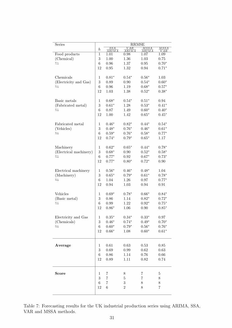
Series RRMSEh SSA

ARIMAV AR

ARIMAMSSA

ARIMAMSSAV AR

Food products 1 1.01 0.98 1.07 1.09(Chemical) 3 1.00 1.36 1.03 0.75¿ 6 0.96 1.37 0.95 0.70∗

12 0.95 1.32 0.94 0.71∗

Chemicals 1 0.81∗ 0.54∗ 0.56∗ 1.03(Electricity and Gas) 3 0.89 0.90 0.54∗ 0.60∗

¿ 6 0.96 1.19 0.68∗ 0.57∗

12 1.03 1.38 0.52∗ 0.38∗

Basic metals 1 0.68∗ 0.54∗ 0.51∗ 0.94(Fabricated metal) 3 0.61∗ 1.28 0.53∗ 0.41∗

¿ 6 0.87 1.49 0.60∗ 0.40∗

12 1.00 1.42 0.65∗ 0.45∗

Fabricated metal 1 0.46∗ 0.82∗ 0.44∗ 0.54∗

(Vehicles) 3 0.48∗ 0.76∗ 0.46∗ 0.61∗

¿ 6 0.59∗ 0.76∗ 0.58∗ 0.77∗

12 0.74∗ 0.79∗ 0.65∗ 1.17

Machinery 1 0.62∗ 0.65∗ 0.44∗ 0.78∗

(Electrical machinery) 3 0.68∗ 0.90 0.52∗ 0.58∗

¿ 6 0.77∗ 0.92 0.67∗ 0.73∗

12 0.77∗ 0.80∗ 0.72∗ 0.90

Electrical machinery 1 0.56∗ 0.46∗ 0.48∗ 1.04(Machinery) 3 0.65∗ 0.79∗ 0.61∗ 0.78∗

¿ 6 1.04 1.26 0.97 0.77∗

12 0.94 1.03 0.94 0.91

Vehicles 1 0.69∗ 0.78∗ 0.66∗ 0.84∗

(Basic metal) 3 0.86 1.14 0.82∗ 0.72∗

¿ 6 0.99 1.22 0.92∗ 0.75∗

12 0.86∗ 1.06 0.90 0.85∗

Electricity and Gas 1 0.35∗ 0.34∗ 0.33∗ 0.97(Chemicals) 3 0.46∗ 0.74∗ 0.49∗ 0.70∗

¿ 6 0.60∗ 0.79∗ 0.56∗ 0.76∗

12 0.66∗ 1.08 0.60∗ 0.61∗

Average 1 0.61 0.63 0.53 0.853 0.69 0.99 0.62 0.636 0.86 1.14 0.76 0.6612 0.89 1.11 0.82 0.74

Score 1 7 8 7 53 7 5 7 86 7 3 8 812 6 2 8 7

Table 7: Forecasting results for the UK industrial production series using ARIMA, SSA,VAR and MSSA methods.

31

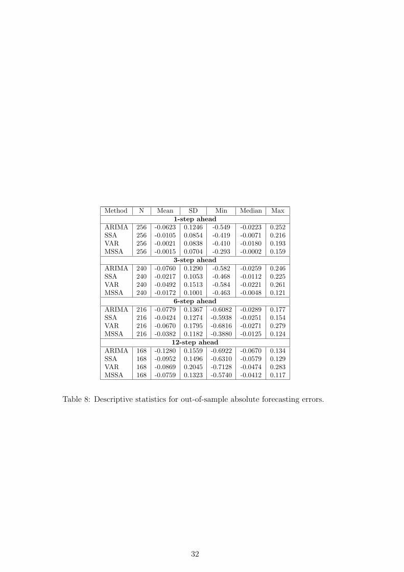
Method N Mean SD Min Median Max1-step ahead

ARIMA 256 -0.0623 0.1246 -0.549 -0.0223 0.252SSA 256 -0.0105 0.0854 -0.419 -0.0071 0.216VAR 256 -0.0021 0.0838 -0.410 -0.0180 0.193MSSA 256 -0.0015 0.0704 -0.293 -0.0002 0.159

3-step aheadARIMA 240 -0.0760 0.1290 -0.582 -0.0259 0.246SSA 240 -0.0217 0.1053 -0.468 -0.0112 0.225VAR 240 -0.0492 0.1513 -0.584 -0.0221 0.261MSSA 240 -0.0172 0.1001 -0.463 -0.0048 0.121

6-step aheadARIMA 216 -0.0779 0.1367 -0.6082 -0.0289 0.177SSA 216 -0.0424 0.1274 -0.5938 -0.0251 0.154VAR 216 -0.0670 0.1795 -0.6816 -0.0271 0.279MSSA 216 -0.0382 0.1182 -0.3880 -0.0125 0.124

12-step aheadARIMA 168 -0.1280 0.1559 -0.6922 -0.0670 0.134SSA 168 -0.0952 0.1496 -0.6310 -0.0579 0.129VAR 168 -0.0869 0.2045 -0.7128 -0.0474 0.283MSSA 168 -0.0759 0.1323 -0.5740 -0.0412 0.117

Table 8: Descriptive statistics for out-of-sample absolute forecasting errors.

32

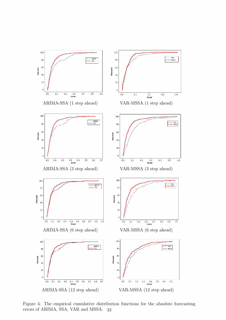
ARIMA-SSA (1 step ahead) VAR-MSSA (1 step ahead)

ARIMA-SSA (3 step ahead) VAR-MSSA (3 step ahead)

ARIMA-SSA (6 step ahead) VAR-MSSA (6 step ahead)

ARIMA-SSA (12 step ahead) VAR-MSSA (12 step ahead)

Figure 4: The empirical cumulative distribution functions for the absolute forecastingerrors of ARIMA, SSA, VAR and MSSA. 33

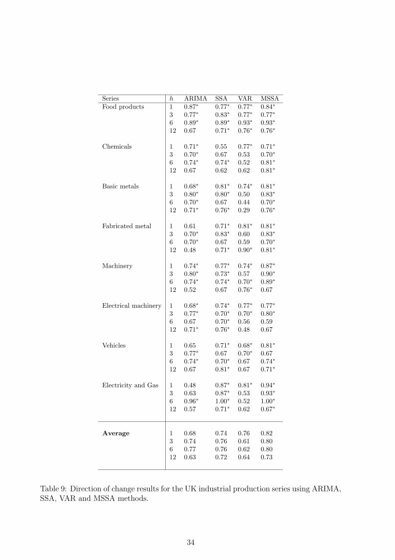
Series h ARIMA SSA VAR MSSAFood products 1 0.87∗ 0.77∗ 0.77∗ 0.84∗

3 0.77∗ 0.83∗ 0.77∗ 0.77∗

6 0.89∗ 0.89∗ 0.93∗ 0.93∗

12 0.67 0.71∗ 0.76∗ 0.76∗

Chemicals 1 0.71∗ 0.55 0.77∗ 0.71∗

3 0.70∗ 0.67 0.53 0.70∗

6 0.74∗ 0.74∗ 0.52 0.81∗

12 0.67 0.62 0.62 0.81∗

Basic metals 1 0.68∗ 0.81∗ 0.74∗ 0.81∗

3 0.80∗ 0.80∗ 0.50 0.83∗

6 0.70∗ 0.67 0.44 0.70∗

12 0.71∗ 0.76∗ 0.29 0.76∗

Fabricated metal 1 0.61 0.71∗ 0.81∗ 0.81∗

3 0.70∗ 0.83∗ 0.60 0.83∗

6 0.70∗ 0.67 0.59 0.70∗

12 0.48 0.71∗ 0.90∗ 0.81∗

Machinery 1 0.74∗ 0.77∗ 0.74∗ 0.87∗

3 0.80∗ 0.73∗ 0.57 0.90∗

6 0.74∗ 0.74∗ 0.70∗ 0.89∗

12 0.52 0.67 0.76∗ 0.67

Electrical machinery 1 0.68∗ 0.74∗ 0.77∗ 0.77∗

3 0.77∗ 0.70∗ 0.70∗ 0.80∗

6 0.67 0.70∗ 0.56 0.5912 0.71∗ 0.76∗ 0.48 0.67

Vehicles 1 0.65 0.71∗ 0.68∗ 0.81∗

3 0.77∗ 0.67 0.70∗ 0.676 0.74∗ 0.70∗ 0.67 0.74∗

12 0.67 0.81∗ 0.67 0.71∗

Electricity and Gas 1 0.48 0.87∗ 0.81∗ 0.94∗

3 0.63 0.87∗ 0.53 0.93∗

6 0.96∗ 1.00∗ 0.52 1.00∗

12 0.57 0.71∗ 0.62 0.67∗

Average 1 0.68 0.74 0.76 0.823 0.74 0.76 0.61 0.806 0.77 0.76 0.62 0.8012 0.63 0.72 0.64 0.73

Table 9: Direction of change results for the UK industrial production series using ARIMA,SSA, VAR and MSSA methods.

34

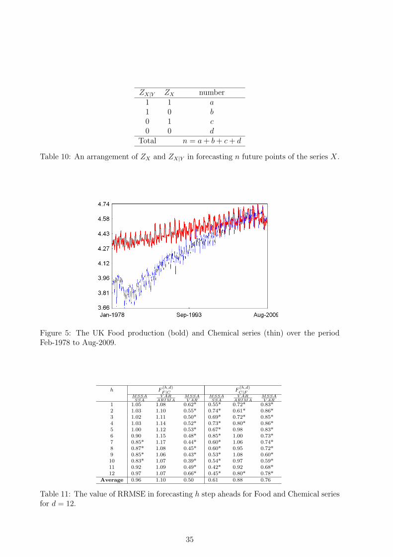
ZX|Y ZX number1 1 a1 0 b0 1 c0 0 d

Total n = a + b + c + d

Table 10: An arrangement of ZX and ZX|Y in forecasting n future points of the series X.

Figure 5: The UK Food production (bold) and Chemical series (thin) over the periodFeb-1978 to Aug-2009.

h F(h,d)F |C F

(h,d)C|F

MSSASSA

V ARARIMA

MSSAV AR

MSSASSA

V ARARIMA

MSSAV AR

1 1.05 1.08 0.62* 0.55* 0.72* 0.83*2 1.03 1.10 0.55* 0.74* 0.61* 0.86*3 1.02 1.11 0.50* 0.69* 0.72* 0.85*4 1.03 1.14 0.52* 0.73* 0.80* 0.86*5 1.00 1.12 0.53* 0.67* 0.98 0.83*6 0.90 1.15 0.48* 0.85* 1.00 0.73*7 0.85* 1.17 0.44* 0.60* 1.06 0.74*8 0.87* 1.08 0.45* 0.60* 0.95 0.72*9 0.85* 1.06 0.43* 0.53* 1.08 0.60*10 0.83* 1.07 0.39* 0.54* 0.97 0.59*11 0.92 1.09 0.49* 0.42* 0.92 0.68*12 0.97 1.07 0.66* 0.45* 0.80* 0.78*

Average 0.96 1.10 0.50 0.61 0.88 0.76

Table 11: The value of RRMSE in forecasting h step aheads for Food and Chemical seriesfor d = 12.

35

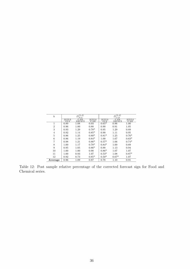
h D(h,d)F |C D

(h,d)C|F

MSSASSA

V ARARIMA

MSSAV AR

MSSASSA

V ARARIMA

MSSAV AR

1 0.89 1.08 0.93 0.65* 0.96 1.002 0.96 1.00 0.88 0.90 0.91 1.053 0.93 1.29 0.78* 0.95 1.29 0.894 0.92 1.14 0.85* 0.90 1.11 0.955 0.96 1.25 0.80* 0.81* 1.25 0.76*6 0.96 1.19 0.84* 1.00 1.67 0.63*7 0.98 1.21 0.86* 0.57* 1.06 0.74*8 1.00 1.17 0.78* 0.84* 1.00 0.899 0.95 1.05 0.86* 0.88 1.13 0.9410 1.00 1.00 0.90 0.86* 1.07 1.0711 1.00 0.93 1.07 0.53* 1.08 0.87*12 0.92 0.73 0.85* 0.50* 0.67* 1.07

Average 0.96 1.09 0.87 0.78 1.10 0.91

Table 12: Post sample relative percentage of the corrected forecast sign for Food andChemical series.

36

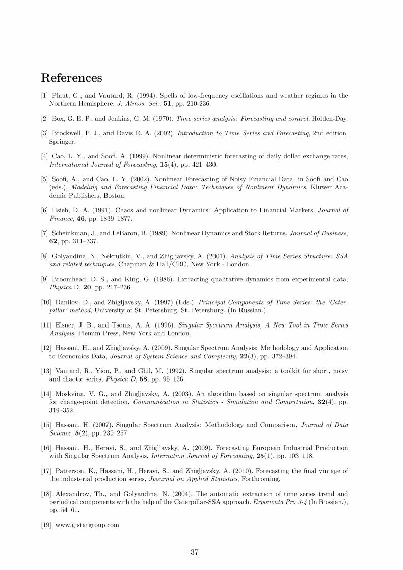
References

[1] Plaut, G., and Vautard, R. (1994). Spells of low-frequency oscillations and weather regimes in theNorthern Hemisphere, J. Atmos. Sci., 51, pp. 210-236.

[2] Box, G. E. P., and Jenkins, G. M. (1970). Time series analysis: Forecasting and control, Holden-Day.

[3] Brockwell, P. J., and Davis R. A. (2002). Introduction to Time Series and Forecasting, 2nd edition.Springer.

[4] Cao, L. Y., and Soofi, A. (1999). Nonlinear deterministic forecasting of daily dollar exchange rates,International Journal of Forecasting, 15(4), pp. 421–430.

[5] Soofi, A., and Cao, L. Y. (2002). Nonlinear Forecasting of Noisy Financial Data, in Soofi and Cao(eds.), Modeling and Forecasting Financial Data: Techniques of Nonlinear Dynamics, Kluwer Aca-demic Publishers, Boston.

[6] Hsieh, D. A. (1991). Chaos and nonlinear Dynamics: Application to Financial Markets, Journal ofFinance, 46, pp. 1839–1877.

[7] Scheinkman, J., and LeBaron, B. (1989). Nonlinear Dynamics and Stock Returns, Journal of Business,62, pp. 311–337.

[8] Golyandina, N., Nekrutkin, V., and Zhigljavsky, A. (2001). Analysis of Time Series Structure: SSAand related techniques, Chapman & Hall/CRC, New York - London.

[9] Broomhead, D. S., and King, G. (1986). Extracting qualitative dynamics from experimental data,Physica D, 20, pp. 217–236.

[10] Danilov, D., and Zhigljavsky, A. (1997) (Eds.). Principal Components of Time Series: the ‘Cater-pillar’ method, University of St. Petersburg, St. Petersburg. (In Russian.).

[11] Elsner, J. B., and Tsonis, A. A. (1996). Singular Spectrum Analysis, A New Tool in Time SeriesAnalysis, Plenum Press, New York and London.

[12] Hassani, H., and Zhigljavsky, A. (2009). Singular Spectrum Analysis: Methodology and Applicationto Economics Data, Journal of System Science and Complexity, 22(3), pp. 372–394.

[13] Vautard, R., Yiou, P., and Ghil, M. (1992). Singular spectrum analysis: a toolkit for short, noisyand chaotic series, Physica D, 58, pp. 95–126.

[14] Moskvina, V. G., and Zhigljavsky, A. (2003). An algorithm based on singular spectrum analysisfor change-point detection, Communication in Statistics - Simulation and Computation, 32(4), pp.319–352.

[15] Hassani, H. (2007). Singular Spectrum Analysis: Methodology and Comparison, Journal of DataScience, 5(2), pp. 239–257.

[16] Hassani, H., Heravi, S., and Zhigljavsky, A. (2009). Forecasting European Industrial Productionwith Singular Spectrum Analysis, Internation Journal of Forecasting, 25(1), pp. 103–118.

[17] Patterson, K., Hassani, H., Heravi, S., and Zhigljavsky, A. (2010). Forecasting the final vintage ofthe industerial production series, Jpournal on Applied Statistics, Forthcoming.

[18] Alexandrov, Th., and Golyandina, N. (2004). The automatic extraction of time series trend andperiodical components with the help of the Caterpillar-SSA approach. Exponenta Pro 3-4 (In Russian.),pp. 54–61.

[19] www.gistatgroup.com

37

[20] Hassani, H., Zhigljavsky, A., Patterson, K., and Soofi, A. (2010). A Comprehensive Causality TestBased on the Singular Spectrum Analysis, Causality in Science, Oxford University press, Forthcoming.

[21] Hassani, H., Dionisio, A., and Ghodsi, M. (2010). The effect of noise reduction in measuring thelinear and nonlinear dependency of financial markets, Nonlinear Analysis: Real World Applications,11(1), pp. 492–502.

[22] Ghodsi, M., Hassani, H., Sanei, S., and Hick, Y. (2009). The use of noise information for detectingtemporomandibular disorder, Biomedical Signal Processing and Control, 4, pp. 79–85.

[23] Hassani, H., Zokaei, M., von Rosen, D., Amiri, S., and Ghodsi, M. (2009). Does Noise ReductionMatter for Curve Fitting in Growth Curve Models?, Computer Methods and Program in Biomedicine,96(3), pp. 173–181.

[24] Osborn, D. R., Heravi, S., and Birchenhall, C. R. (1999). Seasonal unit roots and forecasts of two-digit European industrial production. International Journal of Forecasting, 15, pp. 27–47.

[25] Heravi, S., Osborn, D. R., and Birchenhall, C. R. (2004). Linear Versus Neural Network Forecastsfor European Industrial Production Series. International Journal of Forecasting, 20, pp. 435–446.

[26] Granger, C. W. J. and Lin, J. (1994). Using the Mutual Information Coefficient to Identify Lags inNonlinear Models, Journal of Time Series Analysis, 15, pp. 371-384.

[27] Granger, C. W. J., Maasoumi, E. and Racine, J. (2004). Journal of Time Series Analysis, 25(5), pp.649–669.

[28] DAugostino, R. B., and Stephens, M. A. Eds. (1986). Goodness-of-Fit Techniques, Marcel Dekker.

[29] Doornik, J. A., and Hansen, H. (1994). An Omnibus Test for Univariate and Multivariate Normality.Discussion Paper W4&91, Nuffield College, Oxford, UK.

[30] Shenton, L. R., and Bowman, K. O. (1997). A Bivariate Model for the Distribution of sqrt(b1) andb2, Journal of the American Statistical Association, 72, pp. 206-211.

[31] Darbellay, G. (1998). An Adaptive Histogram Estimator for Mutual Information, UTIA ResearchReport 1889. Academy of Sciences, Prague.

[32] Lee, T. H., White, H., and Granger, C. W. J. (1993). Testing for Neglected Nonlinearity in TimeSeries Models, Journal of Econometrics, 56, pp. 269–290.

[33] McLeod, A. I. and Li, W. K. (1983). Diagnostic checking ARMA time series models using squaredresidual autocorrelations, Journal of Time Series Analysis, 4, pp. 169–176.

[34] Ramsey, J. B. (1969). Tests for specifications errors in classical linear least squares regression analysis.Journal of the Royal Statistical Society, Series B, 31(2), pp. 350–371.

[35] Tsay, R. S. (1986). Non-linearity tests for time series. Biometrika, 73(2), pp. 461–466.

[36] White, H. (1989). Some asymptotic results for learning in single hidden layer feedforward networkmodels. Journal of the American Statistical Association, 84, pp. 1003–1013.

[37] Lhtkepohl, H. (1991). Introduction to Multiple Time Series Analysis. Springer-Verlag, Berlin.

[38] Granger, C. W. J. (1969). Investigating causal relations by econometric models and cross-spectralmethods, Econometrica, 37(3), pp. 424-438.

[39] Granger, C. W. J. (1980). Testing for causality: A personal viewpoint, Journal of Economic Dy-namics and Control, 2, pp. 329–352.

[40] Toda, H. Y., and Phillips, P. C. B. (1991). Vector Autoregressions and Causality: A Theo- reticalOverview and Simulation Study, Econometric Reviews, 13, pp. 259–285.

38

[41] Chu, T., Danks, D. and Glymour, C. (2005). Data Driven Methods for Nonlinear Granger Causality:Climate Teleconnection Mechanisms, Technical report (CMU-PHIL-171).

[42] Hiemstra, C. and Jones, J. D. (1994). Testing for linear and nonlinear Granger causality in the stockprice-volume relation. Journal of Finance, 49(5), pp. 1639-1664.

[43] Diks, C. and Panchenko, V. (2005). A note on the Hiemstra-Jones test for Granger non-causality.Studies in Nonlinear Dynamics and Econometrics, 9 , art. 4.

[44] Bosq, D. (1998). Nonparametric Statistics for Stochastic Processes, (2nd ed), Springer.

[45] Diks, C. and Panchenko, V. (2006). A new statistic and practical guidelines for nonparametricGranger causality testing, Journal of Economic Dynamics and Control, 30, pp. 1647-1669.

[46] Diks, C. and DeGoede, J. (2001). A general nonparametric bootstrap test for Granger causality. In:HW broer, B Krauskopf, G Vegter (Eds.), Global Analysis of Dynamical Systems (Institute of PhysicsPublishing, Bristol, UK), pp. 391–403.

[47] Su, L., and White, H. (2008). A Nonparametric Hellinger Metric Test For Conditional Independence,Econometric Theory, 24(4), pp. 829–864

[48] Diebold F. X., and Mariano R. S. (1995). Comparing predictive accuracy, Journal of Business andEconomic Statistics, 13(3), pp. 253-63

[49] Harvey, D. I., Leybourne, S. J., and Newbold, P. (1997). Testing the Equality of Prediction MeanSquared Errors, International Journal of Forecasting, 13, pp. 281–291.

[50] Ash, J. C. K., Smyth, D. J., and Heravi, S. (1997). The accuracy of OECD forecasts for Japan.Pacific Economic Review, 2(1), pp. 25–44.

[51] Clements, M. P., and Smith, J. (1999). A Monte Carlo investigation of forecasting performance ofemprical SETAR model. Journal of Applied Econometrics, 14, pp. 123–141.

[52] Fleiss, J. L. (1981). Statistical Methods for Rates and Proportions (2nd ed.). New York: Wiley.

[53] Hassani, H., Soofi, A., and Zhigljavsky, A. (2009). Predicting Daily Exchange Rate with SingularSpectrum Analysis. Nonlinear Analysis: Real World Applications, doi:10.1016/j.nonrwa.2009.05.008.

[54] Zhang, G., Patuwo, B. E., and Hu, M. Y. (1998). Forecasting with artificial neural networks: thestate of the art. International Journal of Forecasting, 14, pp. 35-62.

[55] Granger, C. W. J., and Lin, J. (1994). Using the Mutual Information Coefficient to Identify Lags inNonlinear Models, Journal of Time Series Analysis, 15, pp. 371–384.

[56] Darbellay, G., and Wuertz, D. (2000). The Entropy as a Tool for Analysing Statistical Dependence’sin Financial Time Series, Physica A , 287, pp. 429–439.

[57] Dionisio, A., Menezes, R., and Mendes, D. A. (2004). Mutual Information: a Measure of Dependencyfor Nonlinear Time Series, Physica A, 344, pp. 326–329.

[58] Hochberg, Y. (1988). A sharper Bonferroni procedure for multiple tests of significance. Biometrika,75, pp. 800–802.

39