Embed Size (px)
Citation preview

Forecasting Default with the Merton Model
(previously the KMV-Merton Model)
Sreedhar T Bharath
University of Michigan
Ross School of Business
Tyler Shumway
University of Michigan
Ross School of Business
May 16, 2006

Forecasting Default• People have been forecasting default for decades
– Classification: Altman (1968)
– Structural: Merton (1974)
– Hazard: Shumway (2001)
• KMV’s implementation of Merton is interesting
• What does the KMV-Merton model contribute?

KMV and the Merton Model• The KMV-Merton model is based on Merton’s
(1974) bond pricing model
• Developed by KMV corporation in the late 1980s
• Moody’s bought KMV in 2002 for $210 million
• We call the model “KMV-Merton” because it is
a nontrivial extension of Merton – credit KMV
• Others just call it a Merton model
• It is not exactly what MKMV sells - cheap version

The KMV-Merton Model• The model uses market equity, equity volatility,
and the face value of debt to infer the P(default)
• It recognizes that the market value of debt is
unobservable – uses equity to infer debt value
• It is widely used in practice, new in academics
– Vassalou and Xing (2004)
– Duffie, Saita and Wang (2005)
– Campbell, Hilscher and Szilagyi (2005)

Our Paper• We ask how and why KMV-Merton works
• Hypothesis one: πMerton is a sufficient statistic for
predicting default
• Hypothesis two: We need πMerton to construct a
sufficient statistic for predicting default
• We also ask which parts of KMV calculation are
important – can we cut corners?

Assessing KMV-Merton• Our research strategy:
1. Calculate KMV-Merton probabilities (πMerton)
2. Propose a simple, “naive” alternative (πNaive)
3. Estimate hazard models for time to default with
πMerton, πNaive and other variables
4. Look at the out of sample predictive power
5. Estimate regressions for credit default swap
(CDS) probabilities and bond yield spreads

The Merton Model• Merton’s assumptions:
1. One zero-coupon bond with face value F and
maturity T
2. Firm value, V , geometric Brownian motion
3. Other Black-Scholes-Merton assumptions
• Equity, E, is a call option on V with strike equal
to F and maturity of T

Equity in the Merton Model• Equity value is given by the Black-Scholes-Merton
E = V N (d1) − e−rTFN (d2), (1)
d1 =ln(V/F ) + (r + 0.5σ2
V )T
σV T (1/2)(2)
• Debt value is given by the value of a risk-free
bond minus the value of a put written to equity
• Equity volatility follows
σE =(
V
E
)∂E
∂VσV =
(V
E
)N (d1)σV (3)

Two Equations• We have two nonlinear equations,
E = V N (d1) − e−rTFN (d2),
σE =(
V
E
)N (d1)σV
• We can observe E, F , r, T ; we can estimate σE
• We have two unknowns, or unobservables
• Solve the system for V and σV
• This is KMV’s contribution - excellent idea
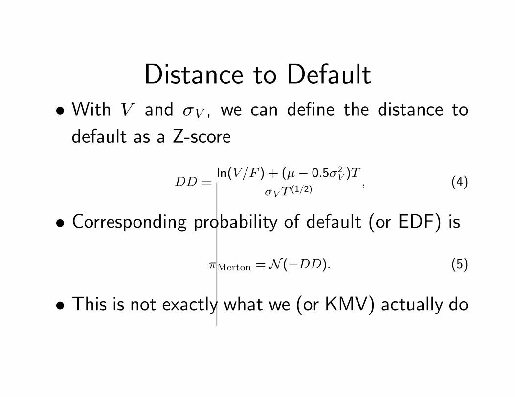
Distance to Default• With V and σV , we can define the distance to
default as a Z-score
DD =ln(V/F ) + (µ − 0.5σ2
V )T
σV T (1/2), (4)
• Corresponding probability of default (or EDF) is
πMerton = N (−DD). (5)
• This is not exactly what we (or KMV) actually do

Iterating on σV
• KMV claims that solving both equations simulta-
neously gives bad results
• Instead we (they) start with an initial σV
• Then we solve the BS equation for V given E
each day for the previous year, using our σV
• We take the resulting time-series of V and calcu-
late a new σV and µ
• We iterate in this way until σV converges

Naive Alternative• We want to construct a measure that is similar to
πMerton without solving equations and iterating
• Somewhat arbitrarily, we define:– Naive V = E + F
– Naive σV = [E/(E + F )]σE + [F/(E + F )](0.05 + 0.25 ∗ σE)
– Naive µ = rit−1
• We calculate naive DD similarly to DD, and we
calculate the corresponding πNaive
• This naive probability is simple to figure
• It captures the form and information of πMerton

Hazard Models• Having defined πMerton and πNaive, we need to
determine which is a better forecaster
• We use the Cox proportional hazard model with
time-varying covariates to assess the models
• The hazard rate is the conditional probability of
failure at time t given survival until time t

Proportional Hazard Model• The proportional hazard model stipulates that
λ(t) = φ(t)[exp(x(t)′β)], (6)
• We use standard techniques to estimate β
• Hazard models are probably the current state of
the art for reduced form default models
– Shumway (2001), Chava and Jarrow (2004)

MKMV vs Our Implementation• We do not do everything exactly like KMV
– Moody’s KMV uses proprietary KV model
– Uses historical data to define CDF of πMerton
– May use a proprietary formula to get F
• While we do not exactly match Moody’s KMV,
we match academic applications
• We can compare to some published KMV data
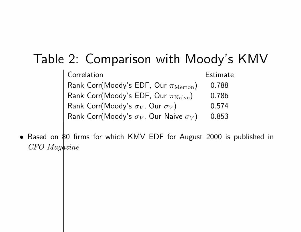
Table 2: Comparison with Moody’s KMVCorrelation Estimate
Rank Corr(Moody’s EDF, Our πMerton) 0.788
Rank Corr(Moody’s EDF, Our πNaive) 0.786
Rank Corr(Moody’s σV , Our σV ) 0.574
Rank Corr(Moody’s σV , Our Naive σV ) 0.853
• Based on 80 firms for which KMV EDF for August 2000 is published in
CFO Magazine

Data• We take all firms from CRSP/Compustat from
1980 through 2003
• We collect defaults from Altman and Moody’s
• Sample has 1,016,552 firm-months, 1449 defaults
• Set T = 1, F = debt in current liabilities + 1/2
of long-term debt
• Previous returns are from CRSP - past year
• Winsorize most variables at 1% and 99%
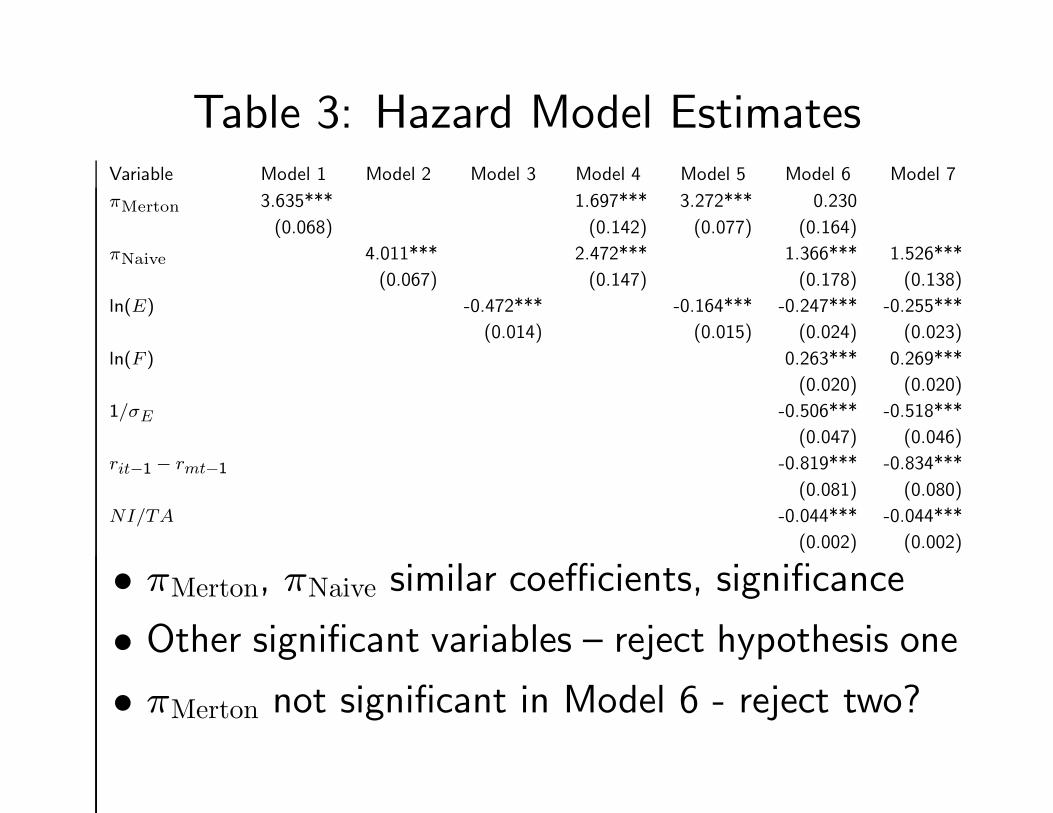
Table 3: Hazard Model EstimatesVariable Model 1 Model 2 Model 3 Model 4 Model 5 Model 6 Model 7
πMerton 3.635*** 1.697*** 3.272*** 0.230
(0.068) (0.142) (0.077) (0.164)
πNaive 4.011*** 2.472*** 1.366*** 1.526***
(0.067) (0.147) (0.178) (0.138)
ln(E) -0.472*** -0.164*** -0.247*** -0.255***
(0.014) (0.015) (0.024) (0.023)
ln(F ) 0.263*** 0.269***
(0.020) (0.020)
1/σE -0.506*** -0.518***
(0.047) (0.046)
rit−1 − rmt−1 -0.819*** -0.834***
(0.081) (0.080)
NI/TA -0.044*** -0.044***
(0.002) (0.002)
• πMerton, πNaive similar coefficients, significance
• Other significant variables – reject hypothesis one
• πMerton not significant in Model 6 - reject two?
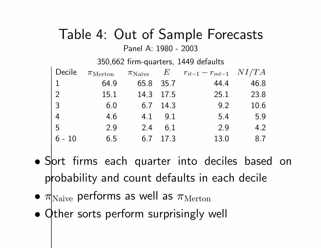
Table 4: Out of Sample ForecastsPanel A: 1980 - 2003
350,662 firm-quarters, 1449 defaultsDecile πMerton πNaive E rit−1 − rmt−1 NI/TA
1 64.9 65.8 35.7 44.4 46.8
2 15.1 14.3 17.5 25.1 23.8
3 6.0 6.7 14.3 9.2 10.6
4 4.6 4.1 9.1 5.4 5.9
5 2.9 2.4 6.1 2.9 4.2
6 - 10 6.5 6.7 17.3 13.0 8.7
• Sort firms each quarter into deciles based on
probability and count defaults in each decile
• πNaive performs as well as πMerton
• Other sorts perform surprisingly well
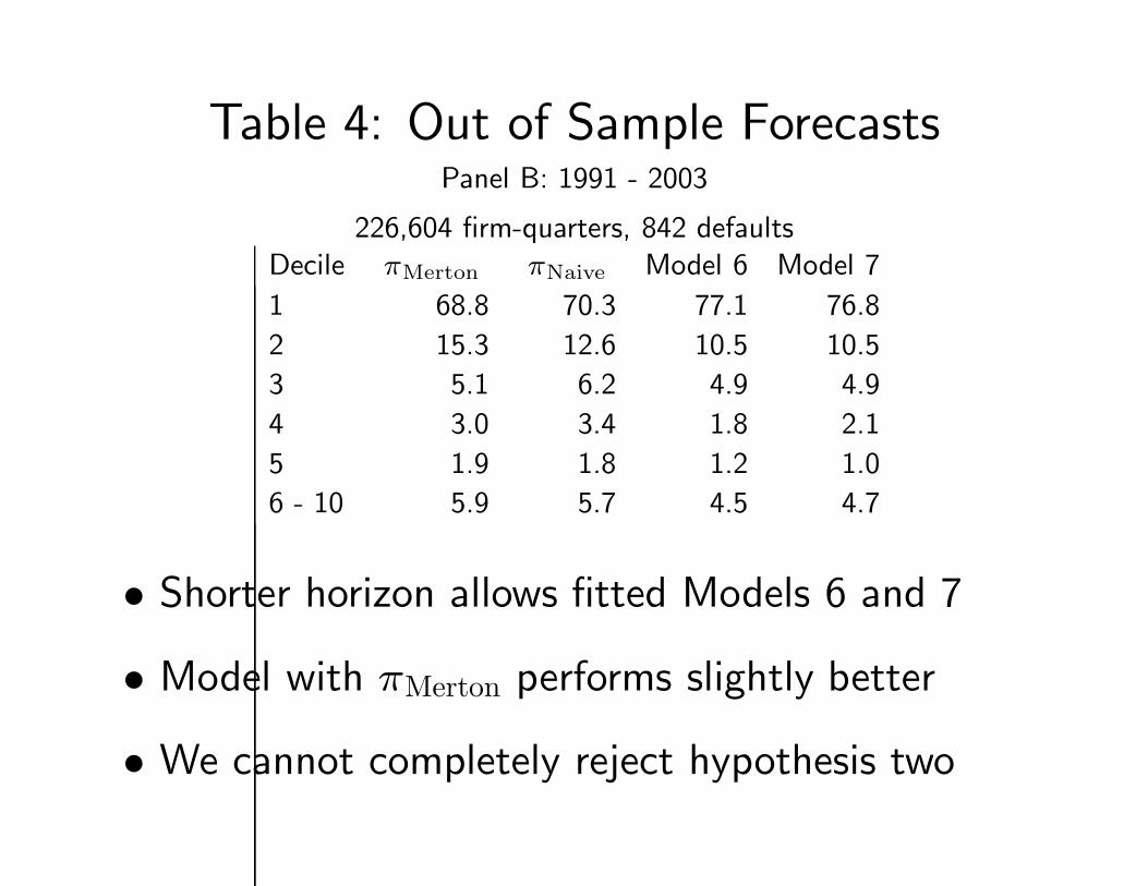
Table 4: Out of Sample ForecastsPanel B: 1991 - 2003
226,604 firm-quarters, 842 defaultsDecile πMerton πNaive Model 6 Model 7
1 68.8 70.3 77.1 76.8
2 15.3 12.6 10.5 10.5
3 5.1 6.2 4.9 4.9
4 3.0 3.4 1.8 2.1
5 1.9 1.8 1.2 1.0
6 - 10 5.9 5.7 4.5 4.7
• Shorter horizon allows fitted Models 6 and 7
• Model with πMerton performs slightly better
• We cannot completely reject hypothesis two

Table 5: Alternative PredictorsPanel C: Out of Sample Forecasts
Decile πµ=rMerton πsimul
Merton πimpσMerton πMerton πNaive
1 60.0 65.1 84.1 80.7 83.0
2 17.7 15.0 8.0 9.1 9.1
3 8.0 7.7 4.6 3.4 5.7
4 4.1 3.4 0.0 5.7 1.1
5 3.4 3.2 1.1 0.0 0.0
6 - 10 6.8 5.6 2.2 1.1 1.1
Defaults 1,449 1,449 88 88 88
Firm-Quarters 350,662 350,662 36,274 36,274 36,274
• πµ=rMerton sets µ = r, performs worse
• πsimulMerton avoids iteration, performs as well
• πimpσMerton uses option-implied σE, performs well

Table 6: CDS Spread RegressionsDependent Variable: πCDS
Variable Model 1 Model 2 Model 3 Model 4
Const. .03∗∗∗ .03∗∗∗ .03∗∗∗ .16∗∗∗(.0005) (.0004) (.0004) (.007)
πMerton .05∗∗∗ -0.001 .009∗∗(.004) (.003) (.004)
πnaive .13∗∗∗ .13∗∗∗ .06∗∗∗(.007) (.008) (.008)
ln(E) -.007∗∗∗(.0005)
ln(F ) .003∗∗∗(.0006)
1/σE -0.014∗∗∗(.0007)
rit−1 -0.0012(.001)
Obs. 3833 3833 3833 3833
R2 0.10 0.26 0.26 0.40
• Including πNaive makes πMerton lose significance

Table 7: Bond Yield Spread RegressionsDependent Variable: Bond Yield Spread
Variable Model 1 Model 2 Model 3 Model 4 Model 5 Model 6
Const. 125.77∗∗∗ 118.27∗∗∗ 126.2∗∗∗ 153.11∗∗∗ 147.28∗∗∗ 153.8∗∗∗(16.55) (16.59) (16.59) (17.43) (17.36) (17.46)
Omitted regressors – See the table in the paper
πNaive .5∗∗∗ .49∗∗∗ .63∗∗∗ .6∗∗∗(.03) (.03) (.04) (.04)
πMerton .08∗∗∗ .007 .19∗∗∗ .1∗∗∗(.008) (.007) (.02) (.01)
Rating Dummies Yes Yes Yes Yes Yes Yes
Year Dummies Yes Yes Yes Yes Yes Yes
Industry Dummies Yes Yes Yes Yes Yes Yes
Obs. 61776 61776 61776 51831 51831 51831
R2 0.70 0.70 0.70 0.72 0.71 0.72
• Including πNaive makes πMerton lose significance

Conclusion• πMerton is a decent default predictor, however
• We reject hypothesis one – πMerton is not sufficient
• We can almost reject hypothesis two – πMerton is
useful with other predictors
• While the iterative procedure is not useful, the
Z-score functional form is fairly useful
• It would be great to have MKMV data to perform
similar tests - too expensive for us