Forces on Fields

Charles T. Sebens

University of California, San Diego

Forthcoming in Studies in History and

Philosophy of Modern Physics

February 9, 2018

arXiv v.3

Abstract

In electromagnetism, as in Newton’s mechanics, action is always equal to

reaction. The force from the electromagnetic field on matter is balanced by an

equal and opposite force from matter on the field. We generally speak only of

forces exerted by the field, not forces exerted upon the field. But, we should not

be hesitant to speak of forces acting on the field. The electromagnetic field closely

resembles a relativistic fluid and responds to forces in the same way. Analyzing

this analogy sheds light on the inertial role played by the field’s mass, the status

of Maxwell’s stress tensor, and the nature of the electromagnetic field.

1 Introduction

Newton’s third law states that whenever one body exerts a force on a second, the second

body exerts an equal and opposite force on the first. The electromagnetic field exerts

forces on matter via the Lorentz force law. I will argue that matter exerts equal and

opposite forces on the field.

Talk of forces on fields is generally resisted as fields seem too insubstantial to be

acted upon by forces. It would be hard to understand how fields could feel forces if they

had neither masses nor accelerations. Fortunately, fields have both. Fields respond to

forces in much the same way that matter does.

Few authors explicitly reject the idea that matter exerts forces on the electromagnetic

field. Instead, the rejection is implied by conspicuous omission. In deriving and

discussing the conservation of momentum, one speaks freely of the force on matter but

only of the rate of change of the momentum of the electromagnetic field (e.g., Cullwick,

1952; Griffiths, 1999, section 8.2; Rohrlich, 2007, section 4.9).

My primary goal in this article is to argue that Newton’s third law holds in the special

relativistic theory of electromagnetism because the force from the electromagnetic field

on matter is balanced by an equal and opposite force from matter on the field. I show

that the field experiences forces by giving a force law for the electromagnetic field using

1

arX

iv:1

707.

0419

8v3

[ph

ysic

s.hi

st-p

h] 9

Feb

201

8

hydrodynamic equations which describe the flow of the field’s mass (originally studied

by Poincare, 1900). In the course of this analysis I clarify the inertial role played by

the field’s mass—it quantifies the resistance the field itself has to being accelerated. I

also point out that Maxwell’s stress tensor is in fact a momentum flux density tensor,

not—as its title would suggest—a stress tensor, and give the true stress tensor for

the electromagnetic field. Finally, I explore the extent of the resemblance between

the electromagnetic field and a relativistic fluid, asking (i) whether we can replace

Maxwell’s equations with fluid equations, (ii) if it is possible to understand the classical

electromagnetic field as composed of photons, and (iii) how we can attribute proper

mass to the field.

2 Apparent Violation of the Third Law

If one takes charged particles to exert electromagnetic forces directly upon one another at

a distance, violations of Newton’s third law are easy to generate. Consider the following

case (Lange, 2002, section 5.2): There are two particles of equal charge initially held

in place (at rest) and separated by a distance r1. Then, one particle is quickly moved

directly towards the other as depicted in figure 1 so that at time t the distance between

the two particles is r2. Because there is a light-speed delay in the way charged particles

interact with one another, the force that each particle feels from the other at t cannot be

calculated just by looking at what’s going on at t. The force on the stationary particle

at t is calculated by looking at the state of the particle that moved at the time when a

light-speed signal from that particle would just reach the stationary particle at t. At this

earlier time, the particle was a distance r1 from where the stationary particle is at t. The

general law describing how the force on one charge depends on the state of another at an

earlier time is complex,1 but in this simple case where both particles are at rest at the

relevant times, the repulsive force that the stationary particle feels at t has magnitudeq2

r21. Similarly, the force on the particle that moved is calculated by looking at the state

of the stationary particle at a time when the stationary particle was at a distance r2

from where the particle that moved is at t. The repulsive force the particle that moved

feels at t has magnitude q2

r22, opposite but not equal the force on the stationary particle.

As a second example (Griffiths, 1999, section 8.2.1), imagine two particles of equal

charge, both equidistant from the origin and approaching at the same speed. Particle 1

approaches along the x-axis from positive infinity and particle 2 along the y-axis. Both

are guided so that they unerringly follow their straight paths at constant speed. In this

1The law giving the force that one charged particle exerts on another is calculated from the retardedLienard-Wiechert potentials (Griffiths, 1999, chapter 10; Feynman et al. , 1964, section 21-1; Lange,2002, pg. 30; Earman, 2011, section 2). Newton’s third law is violated in this sort of case because weare calculating forces directly between particles, not because of the particular choice to use retardedpotentials in order to do so. If advanced potentials were used instead, a similar violation would arise ifthe swerve were placed in the future instead of the past. If half-retarded half-advanced potentials wereused to calculate the forces between particles, either swerve would be sufficient to generate a violation.

2

Figure 1: The two gray lines represent spacetime trajectories of charged particles.The dotted lines indicate which point one must examine on each particle’s spacetimetrajectory to calculate the force on the other at t—taking into account the light-speeddelay on interactions.

case the electric forces on the two particles are equal and opposite but the magnetic

forces are equal in magnitude but not opposite in direction. The magnetic force on

particle 1 is in the y-direction whereas the magnetic force on 2 is in the x-direction.

According to Griffiths, we should be troubled by this violation because “...the

proof of conservation of momentum rests on the cancellation of internal forces, which

follows from the third law. When you tamper with the third law, you are placing the

conservation of momentum in jeopardy, and there is no principle in physics more sacred

than that.” Griffiths then immediately neutralizes the threat, writing that “Momentum

conservation is rescued in electrodynamics by the realization that the fields themselves

carry momentum.” Feynman et al. (1964, sections 26-2 and 27-6) respond to apparent

violations of the third law in a similar manner. They write that they will leave it to the

reader to worry about whether action is equal to reaction, but point out that momentum

is conserved—provided that the field momentum is included—and seem satisfied with

this resolution of the puzzle.

I believe these responses capture the general attitude of physicists to the apparent

violation of Newton’s third law and they are correct as far as they go. However, by

shifting the focus to conservation of momentum they leave the question of whether

Newton’s third law holds unanswered. Since conservation of momentum has been upheld

and the status of Newton’s third law remains uncertain, one might reasonably conclude

that conservation of momentum is the deeper principle. This common attitude appears

in the Wikipedia (2017) article on Newton’s laws of motion: “Newton used the third

law to derive the law of conservation of momentum; from a deeper perspective, however,

conservation of momentum is the more fundamental idea (derived via Noether’s theorem

from Galilean invariance), and holds in cases where Newton’s third law appears to fail,

3

for instance when force fields as well as particles carry momentum, and in quantum

mechanics.” Lange (2002, pg. 163) gives a more definitive rejection of the third law

as a footnote to his discussion of conservation of energy and momentum, “However,

Newton’s third Law (‘Every action is accompanied by an equal and opposite reaction’)

is still violated, even if fields are real. Bodies do not exert forces on fields; bodies alone

feel forces. Newton’s third law was thus abandoned before relativity theory came on the

scene.”2

Another possible reaction to our quandary is to view the third law as immediately

saved by the fact that momentum is conserved. If force is simply the rate of change

of momentum, then the fact that the amount of momentum in the field is changing

is sufficient to demonstrate that forces act on the field (presumably from matter as

it is the only other actor on the scene). Because momentum is conserved, changes in

momentum must cancel and thus forces must balance—Newton’s third law is preserved.

I think it is ultimately correct that the third law is saved by the fact that forces act

on fields. However, I find this quick version of the argument unsatisfactory. One

reason for dissatisfaction is that although the presence of forces on fields is suggested,

a mathematical account of how forces act on fields is absent. Another problem with

this quick argument is that it begs the question against someone who thinks that the

conservation of momentum is a deeper principle than Newton’s third law and may hold

in cases where Newton’s third law does not, as this argument makes obedience of the

third law an immediate consequence of the conservation of momentum.

Some readers might balk at the idea that forces could act upon the electromagnetic

field because they think that the field is merely a useful tool, not a real thing. If the field

isn’t real, it’s hard to see how either Newton’s third law or the conservation of momentum

could hold (though some clever maneuvers have been made to save Newton’s third law

and conservation of momentum in field-less versions of electromagnetism; see Wheeler &

Feynman, 1949; Lange, 2002, chapter 5; Lazarovici, 2017, section 4.2). Over the years,

much has been said in favor of, and in opposition to, taking the electromagnetic field

to be real. For my purposes here, I would like to avoid entering this debate by simply

assuming a certain resolution—that the field is real—and addressing the status of the

third law given this assumption. Once complete, one might take the story presented

here to provide new reasons for believing the field to be real. But, I will not explicitly

draw them out as this debate is not my focus.

In what follows I will give a more thorough defense of the idea that forces act on

fields and explain how they do so. I take the mark of a force to be the obedience

of something like Newton’s second law, ~F = m~a. However, we continue to speak in

2According to Frisch & Pietsch (2016, pg. 16), Ritz (1908) made a similar point while defending aversion of electromagnetism without an electromagnetic field (in which charged particles act directlyupon one another) and criticizing versions of the theory that include field or aether: “[Ritz] also notesthat a theory presupposing an aether does not obey the equality of action and reaction, since the particledoes not react back when the aether acts on a particle.”

4

terms of forces despite certain modifications to that simple equation. In particular, the

second law can be extended to special relativitistic continuum mechanics. What further

modifications the law can sustain while still counting as a force law is more a choice of

convention than a question of deep metaphysics. Perhaps the best convention is to be

liberal about such modifications and to say that wherever there is change in momentum

there is force. Fortunately, we need not judge such modifications in order to determine

whether the electromagnetic field experiences forces. There are two laws of relativistic

continuum mechanics which might deserve to be called force laws and both are obeyed

by the electromagnetic field. Establishing this requires making sense of an m~a type

reaction of the field to the forces it experiences. We turn to this problem in the next

two sections.

3 The Eulerian Perspective

In extending Newton’s second law from the case of discrete bodies to continuum

mechanics we face a choice as to how to describe the physics. There are two equations

that might deserve to be called “the force law,” an Eulerian and a Lagrangian equation

of motion. In this section, I give an Eulerian force law for the electromagnetic field (13)

by first explaining how one can attribute mass and velocity to the field. The Eulerian

force law makes clear what force matter exerts on the field but obscures the nature of

field-on-field forces. In the next section, I give a Lagrangian force law (22) which clarifies

these forces.

Nonrelativistically, bodies respond to forces according to ~F = m~a where the mass m

quantifies the resistance to acceleration. Relativistically, bodies respond to forces by

~F =d~p

dt=

d

dt(mr~v) , (1)

where ~p = mr~v is the body’s momentum and mr is the velocity-dependent relativistic

mass of the body, related to its proper mass by mr = γm0 with γ =(

1− v2

c2

)− 12

.

(In this article I will use the word “mass” without prefix to mean relativistic—not

proper—mass, as it is relativistic mass which is most central to the analysis here.)

Because the time derivative of mr is taken in (1), mass no longer acts as a simple

constant of proportionality between force and acceleration. To clarify the new way in

which mr quantifies resistance to acceleration in relativistic particle mechanics, the force

law can be rewritten as3

~F − ~v

c2

(~v · ~F

)= mr~a . (2)

If we are interested in the force per unit volume on a continuous distribution of mass

3This alternative form is arrived at by expanding the derivative of γ in (1); see Landau & Lifshitz(1972, pg. 49) for the application to electromagnetic force.

5

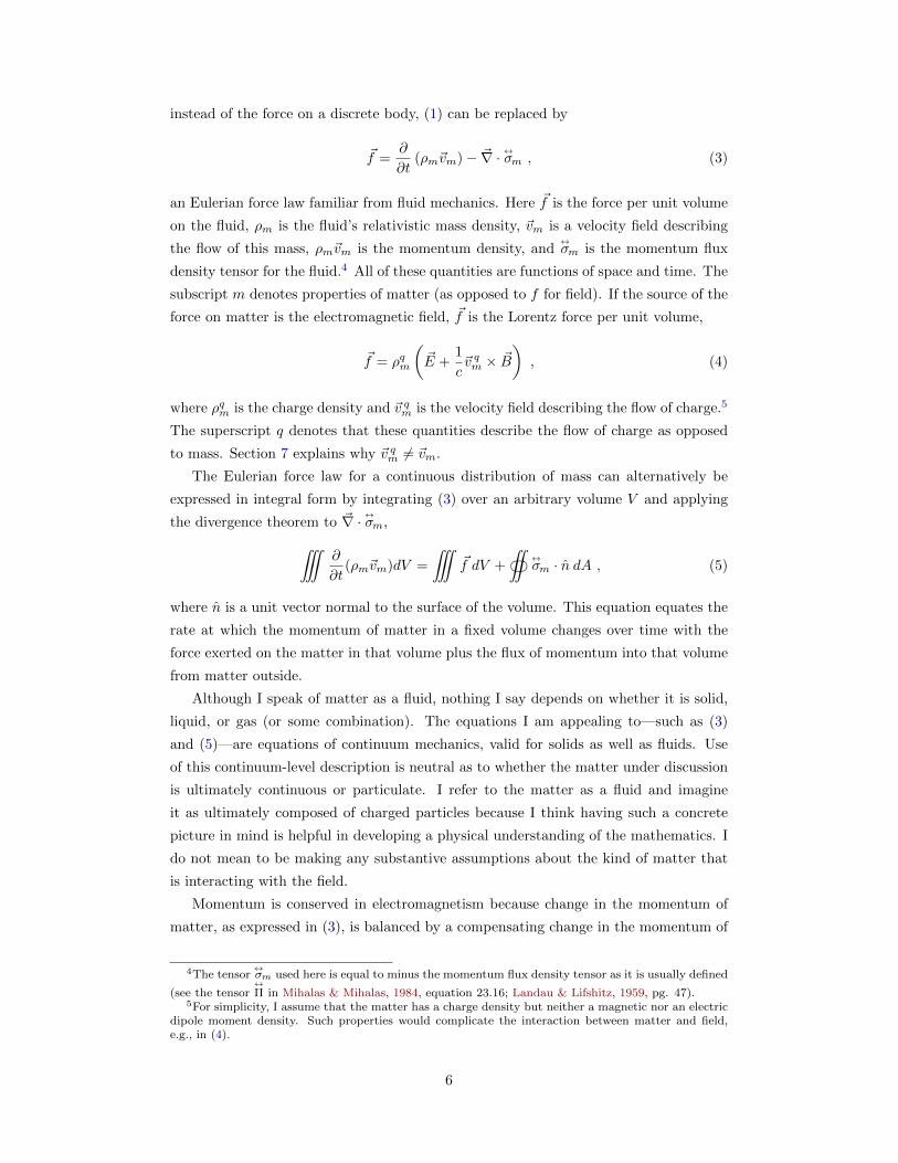
instead of the force on a discrete body, (1) can be replaced by

~f =∂

∂t(ρm~vm)− ~∇ · ↔σm , (3)

an Eulerian force law familiar from fluid mechanics. Here ~f is the force per unit volume

on the fluid, ρm is the fluid’s relativistic mass density, ~vm is a velocity field describing

the flow of this mass, ρm~vm is the momentum density, and↔σm is the momentum flux

density tensor for the fluid.4 All of these quantities are functions of space and time. The

subscript m denotes properties of matter (as opposed to f for field). If the source of the

force on matter is the electromagnetic field, ~f is the Lorentz force per unit volume,

~f = ρqm

(~E +

1

c~v qm × ~B

), (4)

where ρqm is the charge density and ~v qm is the velocity field describing the flow of charge.5

The superscript q denotes that these quantities describe the flow of charge as opposed

to mass. Section 7 explains why ~v qm 6= ~vm.

The Eulerian force law for a continuous distribution of mass can alternatively be

expressed in integral form by integrating (3) over an arbitrary volume V and applying

the divergence theorem to ~∇ · ↔σm,

˚∂

∂t(ρm~vm)dV =

˚~f dV +

‹↔σm · n dA , (5)

where n is a unit vector normal to the surface of the volume. This equation equates the

rate at which the momentum of matter in a fixed volume changes over time with the

force exerted on the matter in that volume plus the flux of momentum into that volume

from matter outside.

Although I speak of matter as a fluid, nothing I say depends on whether it is solid,

liquid, or gas (or some combination). The equations I am appealing to—such as (3)

and (5)—are equations of continuum mechanics, valid for solids as well as fluids. Use

of this continuum-level description is neutral as to whether the matter under discussion

is ultimately continuous or particulate. I refer to the matter as a fluid and imagine

it as ultimately composed of charged particles because I think having such a concrete

picture in mind is helpful in developing a physical understanding of the mathematics. I

do not mean to be making any substantive assumptions about the kind of matter that

is interacting with the field.

Momentum is conserved in electromagnetism because change in the momentum of

matter, as expressed in (3), is balanced by a compensating change in the momentum of

4The tensor↔σm used here is equal to minus the momentum flux density tensor as it is usually defined

(see the tensor↔Π in Mihalas & Mihalas, 1984, equation 23.16; Landau & Lifshitz, 1959, pg. 47).

5For simplicity, I assume that the matter has a charge density but neither a magnetic nor an electricdipole moment density. Such properties would complicate the interaction between matter and field,e.g., in (4).

6

the electromagnetic field,

− ~f =∂

∂t

(~S

c2

)− ~∇ · ↔σf . (6)

This equation can be derived from Maxwell’s equations and the Lorentz force law. The

momentum density of the electromagnetic field is~Sc2 , where ~S is the Poynting vector

which gives the energy flux density,

~S =c

4π~E × ~B . (7)

The (symmetric) tensor↔σf in (6) is the momentum flux density tensor of the

electromagnetic field (also known as the “Maxwell stress tensor,” though I’ll explain

why I dislike that name later) which can be expressed in terms of the electric and

magnetic fields as,

↔σf =

1

4π~E ⊗ ~E +

1

4π~B ⊗ ~B − 1

8π

(E2 +B2

)↔

I , (8)

where ⊗ is the tensor product and↔

I is the identity tensor.6 Here and throughout I use

cgs units.

The equations which quantify the rate at which matter and field momenta change,

(3) and (6), are quite similar. This similarity suggests taking −~f to be a force exerted

by matter on the field, equal and opposite to that of the field on matter. However,

the momentum of the electromagnetic field is an exotic thing and its change does not

obviously resemble the ordinary response of a body to a force. The momentum density

of the electromagnetic field is~Sc2 , not ρm~vm. To show that the field responds to forces

in just the same way that matter does, we must attribute mass and velocity to the field.

The fact that the electromagnetic field has mass can be seen as a result of the

special relativistic equivalence of mass and energy (Einstein, 1906, pg. 204). The field’s

relativistic mass density is equal to the energy density over c2 (by E = mrc2),

ρf =1

8πc2(E2 +B2

). (9)

In general, the (relativistic) mass of matter will vary over time as it exchanges energy

with the electromagnetic field. Attributing the above mass to the electromagnetic field

ensures that the total mass of matter and field is conserved and that the center of mass for

a closed system moves inertially (Einstein, 1906). These considerations provide strong

motivation for saying that the field has mass. But, one might wonder: Does the field act

like it truly has inertial mass, the kind of mass that quantifies resistance to acceleration?

It has often been noted that the field around or inside a body can contribute to the

6In this paper I use the standard expressions for the energy density, momentum density, andmomentum flux density tensor of the electromagnetic field. These quantities together form the field’sfour-dimensional symmetric stress-energy tensor (Jackson, 1999, section 12.10).

7

inertial mass of that body (e.g., consider accelerating a box of radiation or a spherical

charge and its surrounding field; see Whittaker, 1953, pg. 51–52; Griffiths, 2012, section

5). But, this is an indirect way to get at the inertial role played by the mass of the field.

The mass of the field does not merely make it more difficult to accelerate bodies. We

will see that the mass of the field quantifies the resistance to acceleration of the field

itself, just as the mass of a fluid quantifies its resistance to acceleration.

In addition to field mass, we must also make sense of field velocity if we are to

understand forces on fields analogously to forces on matter. The field velocity can be

found by analyzing the flow of energy. The conservation of energy for the electromagnetic

field is expressed by Poynting’s theorem (which, like (6), is derivable from Maxwell’s

equations and the Lorentz force law),

∂

∂t

[1

8π

(E2 +B2

)]+ ~∇ · ~S = −~f · ~v qm

= −[∂

∂t

(ρmc

2)

+ ~∇ ·(ρm~vmc

2)]

. (10)

Here I’ve equated the change in energy of the field with the change in energy of the

matter. The rate of energy transfer between fields and matter, ~f · ~v qm, is equal to ~J · ~Ewhere ~J = ρqm~v

qm is the current density.7 In the second line of (10), ρmc

2 is the energy

density of matter and ρm~vmc2 is the energy flux density. Divide each term in (10) by

c2 and it expresses the conservation of mass. The first term becomes∂ρf∂t by (9). When

integrated over a volume, the second term, ~∇ ·(~Sc2

), gives the rate at which the field’s

mass leaves the volume. If we treated the field as having a velocity, that term would be

~∇ · (ρf~vf ) and the equation would become,

∂ρf∂t

+ ~∇ · (ρf~vf ) =−~f · ~v qmc2

= −[∂ρm∂t

+ ~∇ · (ρm~vm)

]. (11)

This suggests taking the field velocity to be

~vf =~S

ρfc2, (12)

equal to the field momentum density divided by the mass density or, equivalently,

7Being careful, velocity fields like ~v qm only give a coarse-grained description of the velocities of theparticles which compose the fluid. If we assume all of the particles have equal charge, ~v qm assigns to eachpoint in space at each time the average velocity of particles in a very small volume around that pointover a very short period of time (Chapman & Cowling, 1970, section 2.2, Batchelor, 1967, section 1.2).There will be particles with velocities unequal to the mean velocity and they will experience differentLorentz forces. However, because the Lorentz force depends linearly on velocity, the average velocitycan be used to correctly calculate the force per unit volume on the left-hand side of (3) via (4). The rateof energy transfer is also linearly dependent on the velocity (since it is proportional to the dot productof the velocity and the electric field), so the average velocity can be used on the right hand side of thefirst line of (10) as well.

8

equal to the energy flux density divided by the energy density.8 This velocity is

not often discussed, but when it is it goes by the name of the “velocity of energy

transport”—though we could just as well call it the “velocity of (relativistic) mass

transport” (Poincare, 1900, Born & Wolf, 1970, section 14.2.1; Holland, 1993, section

12.6.2; Lange, 2002, box 8.3). The magnitude of the velocity is maximized at c when ~E

is perpendicular to ~B and | ~E| = | ~B|.Using the mass and velocity just introduced, the conservation of momentum equation

for the field (6) looks just like the Eulerian force law for matter (3),

− ~f =∂

∂t(ρf~vf )− ~∇ · ↔σf . (13)

Putting (3) and (13) together, we see that the matter and the field interact like two

overlapping fluids, exerting equal and opposite forces on one another via

∂

∂t(ρf~vf )− ~∇ · ↔σf = −~f

= −[∂

∂t(ρm~vm)− ~∇ · ↔σm

], (14)

and exchanging mass with one another by (11). The interaction between matter and

field is entirely local. The force density ~f on matter at a point in space is balanced

exactly by a force density −~f on the field.

Poincare (1900) proposed that we treat the energy of the electromagnetic field as

a “fictitious fluid,” with mass and velocity essentially as described above, in order to

recover Newton’s third law.9 Poincare sometimes talks as if matter can exert forces on

the electromagnetic field, writing that the forces on a volume must be balanced by the

inertial forces of the matter and the inertial forces of the fictitious fluid. He explains

the way in which the action on matter is matched by an equal and opposite action on

the field as follows: “...since the electromagnetic energy behaves as a fluid which has

inertia, we must conclude that, if any sort of device produces electromagnetic energy

and radiates it in a particular direction, that device must recoil just as a cannon does

when it fires a projectile.” Poincare’s nice story is marred by the fact that he considers

this fluid and its associated mass to be fictitious.10 In the 1900 paper, Poincare wrote

8There are other possible definitions of field velocity that agree on the rate at which field mass leavesany closed volume. However, such alternative definitions would not retain the appropriate relationsbetween velocity, energy flux density, and momentum density. Still, one could cast doubt on thisdefinition of field velocity by challenging the standard expressions for energy flux density and momentumdensity—or even energy density (see Feynman et al. , 1964, section 27-4; Griffiths, 1999, pg. 347,footnote 1; Lange, 2001, 2002; Landau & Lifshitz, 1972, sections 31-33; Jackson, 1999, sections 6.7 and12.10).

9See Weinstein (2012) for a helpful translation of Poincare’s equations into modern notation.10Stein (2014) has argued that this failure to properly appreciate the true possession of inertial mass

by the field was a key reason why Poincare did not arrive at Einstein’s special theory of relativityand symptomatic of his preference for systematizing existing knowledge as opposed to generating novelconsequences. Poincare had hoped for the principle of action and reaction to be satisfied among matteralone and resisted the idea that the ether (or the electromagnetic field) is a real physical entity on apar with ordinary matter.

9

that the fluid should not be considered real because it can be created and destroyed.

That alone cannot be the problem. I was created and I will be destroyed. And yet, I

exist. Perhaps it is only unacceptable for mass to be created and destroyed. However,

from a modern (special relativistic) perspective this is commonplace—the relativistic

mass of ordinary matter changes over time as well (as it exchanges energy with the field

via (11)). If we consider field and matter together, there is no creation or destruction of

mass (just transfer). Poincare has identified a way in which relativistic mass is unlike

non-relativistic mass, but I don’t believe he has given us any reason to think the field,

its mass, or its velocity are not real.

In understanding the resemblance of field to fluid noted by Poincare and explored

in this section, it is helpful to contrast it with a more widely known analogy between

hydrodynamics and electromagnetism utilized by Maxwell (1864) in “On Faraday’s Lines

of Force.” Faraday made great progress understanding electromagnetic phenomena in

terms of electric and magnetic lines of force, precursors to the modern electric and

magnetic fields. Inquiring into “the nature of the lines of magnetic force,” Faraday at one

point puts forward the hypothesis that “physical lines of magnetic force are currents,”

seeing that these lines of force could potentially be understood as describing some kind

of flow (Faraday, 1855, section 3269; Whittaker, 1951, pg. 243; Darrigol, 2000, pg. 112).

Using Faraday’s lines of force, Thomson developed an analogy between electrostatics

and heat flow—in which heat is taken to flow along electric lines of force—and an

analogy between magnetism and hydrodynamics—in which an incompressible fluid is

taken to flow along magnetic lines of force (Harman, 1998, pg. 77–80; Darrigol, 2000,

pg. 114–118, 128–132, 136). Building on the work of Faraday and Thomson, Maxwell

(1864) introduced, as “a purely imaginary substance,” one incompressible fluid that flows

along the electric lines of force and a second fluid that flows along magnetic lines of force

(Whittaker, 1951, pg. 242–244; Harman, 1982, pg. 85–88; Harman, 1998, pg. 87–90;

Darrigol, 2000, pg. 142–147; Lange, 2002, pg. 47–50). These heat and fluid analogies

played an important role in the development of electromagnetic theory as they allowed

Thomson and Maxwell to import mathematical tools and physical insight from better

understood physical theories. It should be clear that Maxwell’s fluid analogy is quite

different from Poincare’s. Poincare treated the electric and magnetic fields together as

a single compressible fluid which flows in the direction of energy flux.

4 The Lagrangian Perspective

Although the Eulerian force law (13) captures the forces from matter on the field well,

it does not make clear what forces the field exerts on itself. To see the problem, consider

integrating (13) over an arbitrary volume V to arrive at an integral form similar to (5),

˚∂

∂t(ρf~vf )dV =

˚ (−~f

)dV +

‹↔σf · n dA . (15)

10

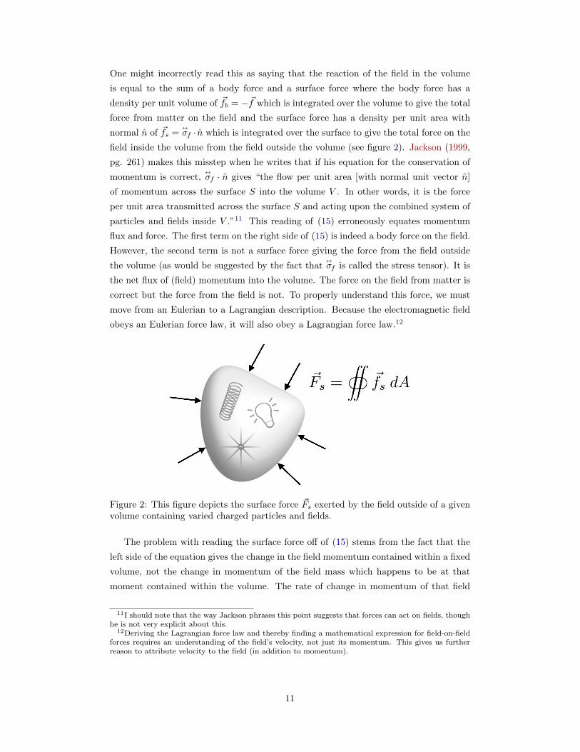
One might incorrectly read this as saying that the reaction of the field in the volume

is equal to the sum of a body force and a surface force where the body force has a

density per unit volume of ~fb = −~f which is integrated over the volume to give the total

force from matter on the field and the surface force has a density per unit area with

normal n of ~fs =↔σf · n which is integrated over the surface to give the total force on the

field inside the volume from the field outside the volume (see figure 2). Jackson (1999,

pg. 261) makes this misstep when he writes that if his equation for the conservation of

momentum is correct,↔σf · n gives “the flow per unit area [with normal unit vector n]

of momentum across the surface S into the volume V . In other words, it is the force

per unit area transmitted across the surface S and acting upon the combined system of

particles and fields inside V .”11 This reading of (15) erroneously equates momentum

flux and force. The first term on the right side of (15) is indeed a body force on the field.

However, the second term is not a surface force giving the force from the field outside

the volume (as would be suggested by the fact that↔σf is called the stress tensor). It is

the net flux of (field) momentum into the volume. The force on the field from matter is

correct but the force from the field is not. To properly understand this force, we must

move from an Eulerian to a Lagrangian description. Because the electromagnetic field

obeys an Eulerian force law, it will also obey a Lagrangian force law.12

Figure 2: This figure depicts the surface force ~Fs exerted by the field outside of a givenvolume containing varied charged particles and fields.

The problem with reading the surface force off of (15) stems from the fact that the

left side of the equation gives the change in the field momentum contained within a fixed

volume, not the change in momentum of the field mass which happens to be at that

moment contained within the volume. The rate of change in momentum of that field

11I should note that the way Jackson phrases this point suggests that forces can act on fields, thoughhe is not very explicit about this.

12Deriving the Lagrangian force law and thereby finding a mathematical expression for field-on-fieldforces requires an understanding of the field’s velocity, not just its momentum. This gives us furtherreason to attribute velocity to the field (in addition to momentum).

11

mass is given byD

Dt

˚ρf~vf dV , (16)

where DDt is the material derivative which gives the rate of change of a quantity while

following the flow (it is also known as the comoving or Lagrangian derivative). Taking

the material derivative inside the integral, (16) becomes

=

˚ [D

Dt(ρf~vf ) + ρf~vf

(~∇ · ~vf

)]dV , (17)

where the second term accounts for the fact that we must consider the deformation

of the volume when calculating the time evolution (see the discussion of the Reynolds

transport theorem in Mihalas & Mihalas, 1984, section 2.1; Slattery, 1999, section 1.3.2;

Belytschko et al. , 2000, sections 3.5.3 and 7.12.1; Gurtin, 1981, section 10). Using the

product rule on the material derivative yields

=

˚ [ρfD~vfDt

+ ~vfDρfDt

+ ρf~vf

(~∇ · ~vf

)]dV . (18)

Expanding the material derivatives gives

=

˚ [ρf∂~vf∂t

+ ρf

(~vf · ~∇

)~vf + ~vf

∂ρf∂t

+ ~vf

(~vf · ~∇

)ρf + ρf~vf

(~∇ · ~vf

)]dV . (19)

This simplifies to

=

˚ [∂

∂t(ρf~vf ) + ~∇ · (ρf ~vf ⊗ ~vf )

]dV . (20)

Using the conservation of momentum (13) to expand the first term, this becomes

=

˚ [−~f + ~∇ ·

(↔σf + ρf ~vf ⊗ ~vf

)]dV . (21)

Applying the divergence theorem, we arrive at

D

Dt

˚ρf~vf dV =

˚ (−~f

)dV +

‹ [↔σf + ρf (~vf ⊗ ~vf )

]· n dA . (22)

This is the Lagrangian force law for the electromagnetic field. The left-hand side is the

response of the electromagnetic field in a region to forces acting on it. The first term on

the right-hand side is the force resulting from interaction with matter. It is equal and

opposite the Lorentz force of the fields on matter. The second term on the right-hand

side is a surface force from the electromagnetic field outside of the volume (figure 2).

By parallel reasoning to the derivation of (22) (except that the force is opposite),

the matter will satisfy

D

Dt

˚ρm~vm dV =

˚~f dV +

‹ [↔σm + ρm (~vm ⊗ ~vm)

]· n dA . (23)

As is clear from comparing (22) and (23), the mass of the electromagnetic field plays

12

exactly the same inertial role in resisting acceleration as does the mass of a relativistic

fluid.

In fluid mechanics, it is↔σm + ρm (~vm ⊗ ~vm), not

↔σm, which gets the name “stress

tensor” because integrating it over a surface gives the force exerted by the matter on

that surface (Mihalas & Mihalas, 1984, equation 23.17; Landau & Lifshitz, 1959, section

15). Similarly, we should call↔σf + ρf (~vf ⊗ ~vf ) the stress tensor for the electromagnetic

field because integrating it over a surface gives the force exerted by the field on that

surface. However, that name is already taken by↔σf itself, the Maxwell stress tensor.13

This is unfortunate. The tensor↔σf is a momentum flux density tensor, not a stress

tensor.14 The tensor↔σf gives the flow of momentum per unit area (when dotted with

the unit normal n) and thus is the correct tensor to use in an Eulerian force law (15)

where we are concerned with determining the flow of momentum in and out of a fixed

volume. But, the force per unit area exerted across the surface is different, given instead

by↔σf + ρf (~vf ⊗ ~vf ). It is this tensor which is used to calculate surface forces in the

Lagrangian force law (22).

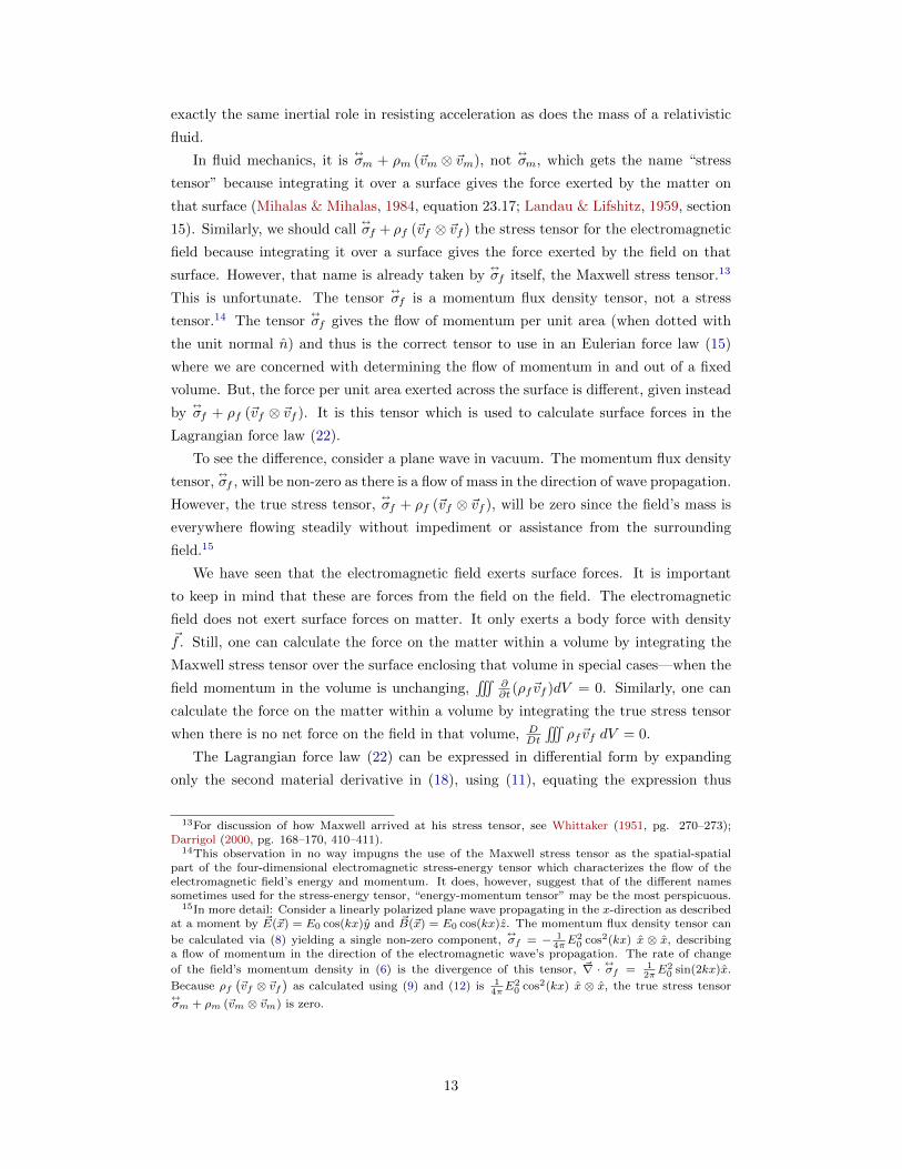
To see the difference, consider a plane wave in vacuum. The momentum flux density

tensor,↔σf , will be non-zero as there is a flow of mass in the direction of wave propagation.

However, the true stress tensor,↔σf + ρf (~vf ⊗ ~vf ), will be zero since the field’s mass is

everywhere flowing steadily without impediment or assistance from the surrounding

field.15

We have seen that the electromagnetic field exerts surface forces. It is important

to keep in mind that these are forces from the field on the field. The electromagnetic

field does not exert surface forces on matter. It only exerts a body force with density

~f . Still, one can calculate the force on the matter within a volume by integrating the

Maxwell stress tensor over the surface enclosing that volume in special cases—when the

field momentum in the volume is unchanging,˝

∂∂t (ρf~vf )dV = 0. Similarly, one can

calculate the force on the matter within a volume by integrating the true stress tensor

when there is no net force on the field in that volume, DDt

˝ρf~vf dV = 0.

The Lagrangian force law (22) can be expressed in differential form by expanding

only the second material derivative in (18), using (11), equating the expression thus

13For discussion of how Maxwell arrived at his stress tensor, see Whittaker (1951, pg. 270–273);Darrigol (2000, pg. 168–170, 410–411).

14This observation in no way impugns the use of the Maxwell stress tensor as the spatial-spatialpart of the four-dimensional electromagnetic stress-energy tensor which characterizes the flow of theelectromagnetic field’s energy and momentum. It does, however, suggest that of the different namessometimes used for the stress-energy tensor, “energy-momentum tensor” may be the most perspicuous.

15In more detail: Consider a linearly polarized plane wave propagating in the x-direction as describedat a moment by ~E(~x) = E0 cos(kx)y and ~B(~x) = E0 cos(kx)z. The momentum flux density tensor can

be calculated via (8) yielding a single non-zero component,↔σf = − 1

4πE2

0 cos2(kx) x ⊗ x, describinga flow of momentum in the direction of the electromagnetic wave’s propagation. The rate of change

of the field’s momentum density in (6) is the divergence of this tensor, ~∇ · ↔σf = 12πE2

0 sin(2kx)x.

Because ρf(~vf ⊗ ~vf

)as calculated using (9) and (12) is 1

4πE2

0 cos2(kx) x ⊗ x, the true stress tensor↔σm + ρm (~vm ⊗ ~vm) is zero.

13

arrived at with (21), and dropping the volume integral,

ρfD~vfDt

= ~∇ ·[↔σf + ρf (~vf ⊗ ~vf )

]− ~f +

~vfc2

(~f · ~v qm

). (24)

This form of the force law resembles (2) where force is related to mass times acceleration

(the force per unit volume on the field being −~f ). This further illustrates that the field’s

mass, ρf , is truly an inertial mass quantifying the field’s resistance to acceleration,

~a =D~vfDt .

Although the analysis thus far has focused on the electromagnetic field, the idea that

forces act on fields is quite general. For any field with well-defined energy and momentum

densities, we can introduce a relativistic mass density which is proportional to the energy

density and a velocity field which is the momentum density divided by the relativistic

mass density. If that field obeys laws of conservation of energy and conservation of

momentum in its interaction with matter (and other fields), then equations of the form

of (11) and (13) will hold. From (13), (22) can be derived.

5 Field as Fluid

In the preceding sections I have argued that Newton’s third law holds in

electromagnetism by showing that the electromagnetic field acts very much like a

relativistic fluid. Here are three questions that might come to mind upon encountering

this analogy: First, can we take these fluid equations as among the fundamental

equations of electromagnetism, supplanting Maxwell’s equations? Second, can we

understand the field’s mass density and velocity as describing properties of a large

number of discrete particles at a coarse-grained level in the way that mass density

and velocity are understood for ordinary fluids? Third, why has the discussion thus

far focused so heavily on relativistic mass instead of proper mass? One section will be

devoted to each of these three questions. These sections can be read in any order or

skipped depending on the reader’s curiosities.

The thorough and consistent similarity between the equations with the f (field)

subscripts and the equations with the m (matter) subscripts suggests that perhaps it

is possible to give an alternative ontology for electromagnetism.16 Electromagnetism

is commonly understood to be a theory describing the interaction between matter and

field. The electromagnetic field appears to be a quite different sort of thing from matter,

described by field variables (such as ~E and ~B, the four-dimensional Faraday tensor

field Fµν , or the electromagnetic four-potential Aµ) evolving in accordance with field

equations. But, the discussion in the previous sections suggests that it may be possible

to treat the field as just more matter, the state of which can be represented by fluid

16As was noted at the end of section 4, other non-electromagnetic fields will generally also resemblefluids in this way. One might take this as evidence that the electromagnetic field is not particularlyfluid-like or as evidence that we may be able to reformulate all field theories as fluid theories.

14

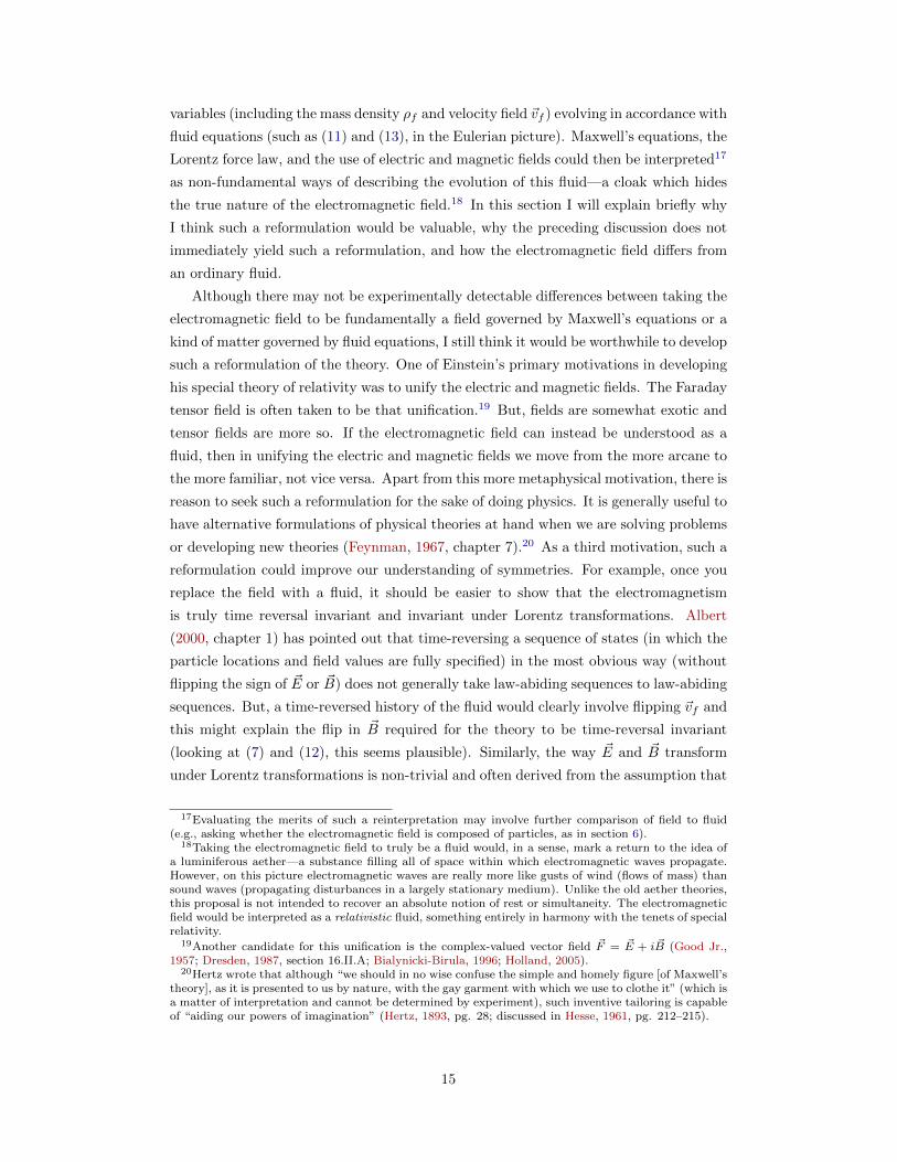
variables (including the mass density ρf and velocity field ~vf ) evolving in accordance with

fluid equations (such as (11) and (13), in the Eulerian picture). Maxwell’s equations, the

Lorentz force law, and the use of electric and magnetic fields could then be interpreted17

as non-fundamental ways of describing the evolution of this fluid—a cloak which hides

the true nature of the electromagnetic field.18 In this section I will explain briefly why

I think such a reformulation would be valuable, why the preceding discussion does not

immediately yield such a reformulation, and how the electromagnetic field differs from

an ordinary fluid.

Although there may not be experimentally detectable differences between taking the

electromagnetic field to be fundamentally a field governed by Maxwell’s equations or a

kind of matter governed by fluid equations, I still think it would be worthwhile to develop

such a reformulation of the theory. One of Einstein’s primary motivations in developing

his special theory of relativity was to unify the electric and magnetic fields. The Faraday

tensor field is often taken to be that unification.19 But, fields are somewhat exotic and

tensor fields are more so. If the electromagnetic field can instead be understood as a

fluid, then in unifying the electric and magnetic fields we move from the more arcane to

the more familiar, not vice versa. Apart from this more metaphysical motivation, there is

reason to seek such a reformulation for the sake of doing physics. It is generally useful to

have alternative formulations of physical theories at hand when we are solving problems

or developing new theories (Feynman, 1967, chapter 7).20 As a third motivation, such a

reformulation could improve our understanding of symmetries. For example, once you

replace the field with a fluid, it should be easier to show that the electromagnetism

is truly time reversal invariant and invariant under Lorentz transformations. Albert

(2000, chapter 1) has pointed out that time-reversing a sequence of states (in which the

particle locations and field values are fully specified) in the most obvious way (without

flipping the sign of ~E or ~B) does not generally take law-abiding sequences to law-abiding

sequences. But, a time-reversed history of the fluid would clearly involve flipping ~vf and

this might explain the flip in ~B required for the theory to be time-reversal invariant

(looking at (7) and (12), this seems plausible). Similarly, the way ~E and ~B transform

under Lorentz transformations is non-trivial and often derived from the assumption that

17Evaluating the merits of such a reinterpretation may involve further comparison of field to fluid(e.g., asking whether the electromagnetic field is composed of particles, as in section 6).

18Taking the electromagnetic field to truly be a fluid would, in a sense, mark a return to the idea ofa luminiferous aether—a substance filling all of space within which electromagnetic waves propagate.However, on this picture electromagnetic waves are really more like gusts of wind (flows of mass) thansound waves (propagating disturbances in a largely stationary medium). Unlike the old aether theories,this proposal is not intended to recover an absolute notion of rest or simultaneity. The electromagneticfield would be interpreted as a relativistic fluid, something entirely in harmony with the tenets of specialrelativity.

19Another candidate for this unification is the complex-valued vector field ~F = ~E + i ~B (Good Jr.,1957; Dresden, 1987, section 16.II.A; Bialynicki-Birula, 1996; Holland, 2005).

20Hertz wrote that although “we should in no wise confuse the simple and homely figure [of Maxwell’stheory], as it is presented to us by nature, with the gay garment with which we use to clothe it” (which isa matter of interpretation and cannot be determined by experiment), such inventive tailoring is capableof “aiding our powers of imagination” (Hertz, 1893, pg. 28; discussed in Hesse, 1961, pg. 212–215).

15

the theory is Lorentz invariant (e.g., Griffiths, 1999, section 12.3.2). One might hope

to derive these transformation rules from less contestable transformation laws for the

fluid.21

If we are to replace the fundamental equations of relativistic electromagnetism with

fluid equations, like (11) and (13), we must introduce additional variables to describe the

state of this fluid beyond those we’ve seen thus far. The Maxwell stress tensor—which is

needed to calculate the dynamics of the fluid using (13) or (22)—cannot be determined

from the mass density and the velocity alone. (Too see this, imagine rotating the electric

and magnetic field together about ~vf . This will generally change↔σf but cannot affect ρf

or ~vf .) Further, even if we have ρf , ~vf , and↔σf at our disposal (which contain the same

information as the four-dimensional stress-energy tensor of the electromagnetic field),

we will not know enough about the field to calculate the force on matter. (Consider

swapping the electric and magnetic fields and multiplying one of the fields by −1. By

inspection of (8), (9), and (12) it is clear that this will not effect ρf , ~vf , or↔σf . But, it will

in general change the forces felt by charged bodies.22) Thus, there must be additional

degrees of freedom characterizing the state of the fluid beyond just ρf and ~vf and they

must include information not present in↔σf . To make this proposal for new fundamental

laws work, one would have to identify appropriate variables to represent these additional

degrees of freedom, physically interpret them, and find additional equations to govern

their time evolution.23 Bialynicki-Birula (1997); Bialynicki-Birula & Bialynicka-Birula

(2003) have devised a way of introducing such additional variables, though the resulting

equations are not simple and the physical interpretation of the new variables is not

entirely clear. Holland (2005) has proposed an alternative way of introducing fluid

variables to describe the electromagnetic field.

As was mentioned in section 3, in describing the matter as a “fluid” I have been

speaking somewhat loosely. The use of a mass density and velocity field obeying

equations like (3), (11), and (23) to describe a substance does not determine whether it

is fluid or solid. Similarly, in asking here whether we might be able to understand the

field as a fluid, I am really asking whether we can understand it using the framework

of continuum mechanics (which encompasses both solid and fluid mechanics). It is

important to recognize that there are important ways in which the electromagnetic field

will not resemble a true fluid.

Consider a constant electric field between two oppositely charged parallel plates

separated from one another by a gap in the x-direction, ~E = Ex. Because there is no

21This potential advantage in understanding symmetries using a fluid ontology is analogous to theadvantage of a fluid ontology for quantum mechanics in understanding symmetries discussed in Sebens(2015, section 12).

22If you knew the rates of change of ρf and ~vf , you could calculate the Lorentz force by (13). But,then this equation would no longer be able to tell you how the field evolves.

23If we think of the field as a fluid of photons, it may be possible to understand the additional degreesof freedom as describing—in aggregate—the spins/polarizations of the photons as this information doesnot seem to be captured by the mass density or velocity of the field.

16

magnetic field, the field velocity is zero. The momentum flux density tensor is

↔σf =

E2

8π 0 0

0 −E2

8π 0

0 0 −E2

8π

, (25)

by (8). As ~vf = 0, the momentum flux density tensor,↔σf , is equal to the stress tensor

for the field,↔σf +ρf (~vf ⊗ ~vf ). The force per unit area with normal n is thus

↔σf · n. If n

points in the y or z-direction, the force is compressive. But, if n points in the x-direction

the force has the opposite sign. The electromagnetic field is sustaining a tensile force

(pulling the two plates towards one another). Solids can sustain such tensile forces

but fluids cannot (Mihalas & Mihalas, 1984, pg. 70). In this way, the electromagnetic

field more closely resembles a solid than a fluid. To see another disanalogy between

the electromagnetic field and a true fluid, take n to point halfway between the x and

y-directions. In this case, the force per unit area,↔σf · n, will not be parallel to n,

indicating the presence of shearing forces. An ordinary fluid cannot sustain such shearing

forces when at rest (Batchelor, 1967, pg. 12–14; Gurtin, 1981, pg. 105; Mihalas &

Mihalas, 1984, pg. 70).

6 Photons and the Classical Electromagnetic Field

Relativistic quantum field theories can either be understood as quantum theories of

relativistic fields or relativistic theories of quantum particles. In particular, the photons

which mediate electromagnetic interactions between charged particles in quantum

electrodynamics may be understood either as field or particle. There is debate about

whether particle or field is more fundamental in quantum field theory, but to some degree

the theory can be interpreted either way. What I would like to explore in this section

is the extent to which we are already able to treat photons as either particle or field at

the classical level.

The mass density and velocity field of a relativistic fluid, ρm and ~vm, describe at

a coarse-grained level the properties of the particles which compose the fluid. Can we

similarly understand the mass density and velocity field of the electromagnetic field as

describing properties of the photons which compose the field? Photons have no proper

mass and always travel at the speed of light. These features make them unusual but not

unsuitable candidates for a fluid-level description.24 Even if each particle is traveling at

c, |~vf | may still be less than the speed of light as ~vf describes the net flow of relativistic

mass and not the actual velocity of any individual particle. Further, (as was discussed

when the field velocity was introduced) |~vf | cannot be greater than c, which we may view

24Also, the mean free path for photons is typically large (light beams generally pass through oneanother undisturbed). So, photons at some location (~x, t) are likely to have velocities far from the meanvelocity ~vf (~x, t) and not to be carried along with the flow. (See Shu, 1992, chapter 1.)

17

as explained by the fact that the field is made of photons each traveling at c. There

is no problem with the field having a non-trivial mass density even if its constituent

particles are massless. Particles without proper mass can still have relativistic mass

and collections of particles without proper mass will generally together have proper

mass—proportional to the energy they posses in their collective center of momentum

frame (see section 7).

Thus far I have focused primarily on the relativistic mass densities of fluids and

fields. But, a relativistic fluid also has a number density and if the electromagnetic

field is composed of particles it seems like it should have one too. Because photons

are quantum particles, we must look to quantum physics to find a number density

for the electromagnetic field. The possibility of finding a well-defined number-density

is threatened by the fact that quantum mechanically there can be a superposition of

different number densities (see Holland, 1993, pg. 545).

It is possible to give a “classical” expression for the photon number density without

considering the full complexities of quantum physics. Consider the electromagnetic field

in vacuum. A natural strategy for finding the photon number density would be to

divide the energy density of the field, ρ Ef (~x) = 18π (| ~E(~x)|2 + | ~B(~x)|2), by the energy

per photon. From quantum physics, we know that the energy of a photon with wave

vector ~k is E = |~k|~c. Because of the dependence on ~k, it is hard to execute that natural

strategy. But, it is possible to divide the energy density by the energy per photon to

arrive at a number density if we work in ~k-space. Integrating this number density over

~k-space gives the total number of photons,

N =

˚|~E(~k)|2 + | ~B(~k)|2

8π|~k|~cd3k , (26)

where~E(~k) and

~B(~k) are the Fourier transformed electric and magnetic fields,25

~E(~k) =

1

(2π)3/2

˚~E(~x)e−i

~k·~xd3x

~B(~k) =

1

(2π)3/2

˚~B(~x)e−i

~k·~xd3x . (27)

If you expand~E(~k) and

~B(~k) in (26) using (27) and perform the integral over ~k, (26)

becomes

N =1

16π3~c

˚˚ ~E(~x) · ~E(~y) + ~B(~x) · ~B(~y)

|~x− ~y|2d3x d3y . (28)

(This method of counting photons was proposed by Zel’dovich, 1966; see also

Bialynicki-Birula, 1996, pg. 318; Avron et al. , 1999.) One can generate a number

25Because the transformed fields are complex-valued, |~E(~k)|2 is shorthand for~E

∗(~k) · ~E(~k).

18

density by simply dropping one of the spatial integrals,

ρNf (~x) =1

16π3~c

˚ ~E(~x) · ~E(~y) + ~B(~x) · ~B(~y)

|~x− ~y|2d3y

=1

16π3~c

[~E(~x) ·

˚ ~E(~x+ ~r)

r2d3r + ~B(~x) ·

˚ ~B(~x+ ~r)

r2d3r

], (29)

with ~r defined as ~y − ~x. It is odd that the density of photons at one point depends

on what’s happening everywhere else (through the spatial integral), but not obviously

unacceptable—figuring out what kind of photons there are at a certain point may require

examining the way the field behaves nearby (nearby field values are most important as

the factor of |~x−~y|2 in the denominator suppresses contributions from distant locations).

To check that (29) is at least a minimally sensible expression, consider the simple

case of a linearly polarized plane wave propagating in the x-direction with ~E(~x) =

E0 cos(kx)y and ~B(~x) = E0 cos(kx)z. The energy density of the plane wave isE2

0

4π cos2(kx) and the energy per photon is k~c. As the reader can confirm, the photon

density derived using (29) isE2

0 cos2(kx)4πk~c , exactly as it should be.

7 Proper Mass Density

In attributing fluid-like properties to the electromagnetic field, we have not yet given it a

proper mass density. The reason for this is that there are a number of oddities involved

in defining the proper mass density for a relativistic fluid. It is no more difficult to define

a proper mass density for the electromagnetic field, but the oddities afflicting the fluid

case are inherited.

There are five densities for a fluid that have come up in our discussion thus far:

charge density, energy density, relativistic mass density, proper mass density, and particle

number density. Corresponding to these five densities are five velocity fields which

describe their flows: ~v qm, ~v Em, ~vmrm , ~vm0

m , and ~vNm . Are any of these five velocity fields

equal to one another? For the most part, no. The only equality that holds in general

is between the velocities describing energy and relativistic mass flow (since energy is

directly proportional to relativistic mass). This velocity, ~v Em = ~vmrm , is the velocity

we have focused on thus far and denoted ~vm (without a superscript). This velocity is

generally not equal to the velocity describing the flow of particle number, ~vNm , because

sometimes energy (and thus relativistic mass) flows as a result of something other than

the bulk motion of particles in the fluid, e.g., when there is heat flux (see Landau &

Lifshitz, 1959, pg. 505). If we add the assumption that the particles which compose

the fluid have equal charge q, then the charge density is q times the number density

and ~v qm is equal to ~vNm (but because ~vm 6= ~vNm , ~v qm will generally differ from ~vm, as was

mentioned in section 3). If the particles have equal proper mass m0 and we assume (as

an idealization) that all of the particles near (~x, t) can be treated (contra footnote 7) as

moving with the same velocity ~vNm (~x, t), then the proper mass density is simply m0 times

19

the number density and, because of this proportionality, the velocity describing the flow

of proper mass, ~vm0m , is equal to the velocity describing the flow of particle number,

~vNm (see Mihalas & Mihalas, 1984, equation 39.5). Relaxing this idealization, the proper

mass density can be defined in two different ways, each of which has undesirable features.

The first method is to tie proper mass density closely to number density, insisting

that the proper mass density is the particle proper mass m0 times the number density

and that ~vNm is, as before, equal to ~vm0m . As number density is locally conserved and

transforms trivially under Lorentz transformations (picking up a factor of γ since it is a

density and length contraction shrinks the volumes over which it is integrated, Mihalas

& Mihalas, 1984, eq. 39.4), proper mass density so defined will inherit these properties.

But, with this definition there is little connection between proper mass density and

energy density (or relativistic mass density). To see why this is so, consider a simple

case in which there is no flow of particle number and no flow of energy, ~vNm = ~v Em = 0.

Because the proper mass of a system in its rest frame is equal to the system’s energy

divided by c2, one might hope that in this state of rest the fluid’s energy density is equal

to the proper mass density times c2. With this definition, that will not be so. The

proper mass density defined as ρm0m = m0 × ρNm does not account for contributions to

the energy in this frame other than the rest mass energies of the particles, such as the

contribution from the heat of the fluid (the energy due the random motion of particles

about their mean velocity).

The second method for defining the proper mass density of a fluid ties it more closely

to relativistic mass density and energy density. The proper mass density is defined

in terms of the energy density, ρ Em = ρmc2, and the momentum density, ρm~vm, by

ρ2mc2−ρ2m|~vm|2 = (ρm0

m )2c2 (taking the relativistic relation between energy, momentum,

and proper mass (E/c)2−|~p|2 = m20c

2, as applied to the densities of these quantities, to be

definitional of proper mass density). From this equation it follows that ρm0m = ρm

γ =ρ Em

γc2

where the velocity that appears in γ is the velocity that describes the flow of relativistic

mass, ~vm. If we consider the fluid at a point from a frame where the momentum density

at that point is zero, the proper mass density will simply be given by the energy density

at that point divided by c2. This definition resolves the problem raised for the previous

definition since all contributions to the energy are included (ρm0m will thus generally

be greater than m0 × ρNm ). If we idealize away the effect of heat by assuming that all

of the particles near (~x, t) have velocity ~vNm (~x, t) and assume that there are no other

contributions to the energy that need to be included beyond the rest mass and kinetic

energies of the particles, then ~vNm = ~vm, the energy density is ρ Em = m0γc2 × ρNm ,

and the rest mass density is exactly ρm0m = m0 × ρNm (the two alternative definitions

agree). On this second definition, local conservation of proper mass cannot be derived

straightforwardly from either conservation of particle number or conservation of energy.

This makes it difficult to find an appropriate velocity ~vm0m to describe the flow of proper

mass.

On neither of the two proposed definitions will integrating the proper mass density

20

of the fluid over the volume occupied by the fluid give the proper mass of the fluid as a

whole. This is because proper mass is not additive. Consider the collection of particles

that compose a gas as described by their positions and velocities, not yet by densities

and velocity fields. Summing the proper masses of the particles will not give the proper

mass of the gas. The proper mass of the gas is found by dividing the energy of the gas

by c2 in the frame where the net momentum of the gas is zero—the rest frame of the

gas (see Lange, 2001, 2002, chapter 8). Similarly, the proper mass of a fluid described

using densities and velocity fields can be determined by integrating the fluid’s energy

density in the frame in which the net momentum of the fluid is zero and dividing by c2.

As with a relativistic fluid, the field’s proper mass density can be defined in two

ways. If we define it as the mass of each particle times the number density and take the

field to be composed of massless photons, then the proper mass density is everywhere

and always zero. Alternatively, we can derive a proper mass density using the relation

(E/c)2− |~p|2 = m20c

2 as applied to the energy, momentum, and proper mass densities of

the field (see Lange, 2002, pg. 244):

ρm0

f =1

4πc2

√1

4(E2 −B2)

2+ ( ~E · ~B)2 . (30)

We saw earlier that the proper mass density of a fluid (defined in this second way)

can be more than the particle mass times the number density, m0 × ρNm , because of

other contributions to the energy—e.g., random particle motion a.k.a. heat. If a fluid is

made of massless particles its proper mass must come entirely from such contributions

as m0 = 0. Note that the proper mass density in (30) is frame-independent26 whereas

the proper mass density for a relativistic fluid of massive particles (similarly defined)

is frame-dependent. With proper mass density as with speed, only fleet-footed photons

manage to appear the same in every frame.27

As was the case for a relativistic fluid, the proper mass of the field as a whole is not

the integral of the proper mass density. Instead, it can be determined by integrating

the field’s energy density in the frame in which the net momentum of the field is zero

and dividing by c2. This method of determining the field’s proper mass raises problems.

26See Lange (2002, pg. 244) alongside Jackson (1999, problem 11.14); Garg (2012, section 161).27In Lange (2002) the guiding question is whether electromagnetic interactions are local. Lange argues

that this turns on the question of whether the electromagnetic field is real. On pg. 247 he summarizeshis case that it is:

“...we tried to use the ontological status of energy and momentum to support the field’sreality ... But this argument ultimately failed when we learned from relativity theory thatenergy and momentum are frame-dependent, and hence unreal. Relativity did, however,reveal [proper] mass to be real. Its ontological status has now come to underwrite theelectromagnetic field’s reality, since the field has turned out to possess [proper] mass.”

The analysis in this section challenges that reasoning. It is true that, as Lange emphasizes, the propermass density of the field as defined by (30) is frame-independent. But, this is a special feature of theelectromagnetic field and thus an odd hook on which to hang its reality. The proper mass density fora relativistic fluid similarly defined will be frame-dependent, and yet we do not doubt whether suchfluids are real. Of course, there is another reason available for taking relativistic fluids to be real: theparticles that compose such fluids have frame-invariant proper masses.

21

There may be no rest frame for the field as a whole (as would happen if, for example,

the field is that of a plane wave traveling at c; see Rohrlich, 1970). To avoid this

problem we can define the proper mass of the field in a particular frame in terms of

the field’s total energy and momentum in that frame by (E/c)2 − |~p|2 = m20c

2. Because

the three-dimensional hyperplane of simultaneity in a moving frame will not agree with

the hyperplane of simultaneity in the original frame and in the gaps between these

hyperplanes there may be an exchange of energy (and momentum) between the field

and matter, the field’s proper mass will end up differing from frame to frame. This can

seem problematic when it is put as a lament that the field’s energy and momentum do

not transform as a four-vector: the inner product of the energy-momentum four-vector

with itself, (E/c)2 − |~p|2 = m20c

2, is frame-dependent. (If there is no matter present

and the field is truly isolated this problem will not arise.28) In response to this second

problem, we can either define the field’s energy, momentum, and proper mass as relative

to a specified hyperplane (Rohrlich, 1970, 1996, 2007) or just note that only when we

speak of matter and field together will energy and momentum transform as a four-vector

and proper mass be frame-invariant (Griffiths & Owen, 1983; Rohrlich, 1996).

8 Conclusion

In electromagnetism, as in Newton’s mechanics, action is always equal to reaction. The

force from the electromagnetic field on matter is balanced by an equal and opposite

force from matter on the field. The response of the field to this force can be given in

Eulerian (13), (15) or Lagrangian (22), (24) form. These equations perfectly match

those that govern a relativistic fluid. From examination of the analogy it is clear that

the mass of the field plays exactly the same inertial role as the mass of a fluid and also

that the Maxwell stress tensor is really a momentum flux density tensor, not a stress

tensor. This perfect match of field and fluid equations suggests that it may be possible

to reinterpret the electromagnetic field as a fluid of photons.

Acknowledgments

Thank you to Craig Callender, Dirk-Andre Deckert, Mario Hubert, and Mark Lange

for valuable discussions and helpful feedback on drafts of the paper. Special thanks to

Erik Curiel, Dennis Lehmkuhl, and James Weatherall. Thanks also to the anonymous

referees who provided useful comments on the paper.

28This can be put another way: the total energy and momentum of the field will transform as afour-vector if there is no matter present because the divergence of the stress-energy tensor is zeroeverywhere (Jackson, 1999, problem 12.18).

22

References

Albert, David. 2000. Time and Chance. Harvard University Press.

Avron, J E, Berg, E, Goldsmith, D, & Gordon, A. 1999. Is the Number of Photons a

Classical Invariant? European Journal of Physics, 20(3), 153–159.

Batchelor, G. K. 1967. An Introduction to Fluid Dynamics. Cambridge University Press.

Belytschko, Ted, Liu, Wing Kam, & Moran, Brian. 2000. Nonlinear Finite Elements for

Continua and Structures. John Wiley & Sons.

Bialynicki-Birula, Iwo. 1996. The Photon Wave Function. Pages 313–322 of: Eberly,

Joseph H., Mandel, Leonard, & Wolf, Emil (eds), Coherence and Quantum Optics

VII: Proceedings of the Seventh Rochester Conference on Coherence and Quantum

Optics, held at the University of Rochester, June 7–10, 1995. Springer.

Bialynicki-Birula, Iwo. 1997. Hydrodynamics of Relativistic Probability Flows. Pages

64–71 of: Infeld, E., Zelazny, R., & Galkowski, A. (eds), Nonlinear Dynamics, Chaotic

and Complex Systems: Proceedings of an International Conference Held in Zakopane,

Poland, November 7-12 1995, Plenary Invited Lectures. Cambridge University Press.

Bialynicki-Birula, Iwo, & Bialynicka-Birula, Zofia. 2003. Vortex Lines of the

Electromagnetic Field. Physical Review A, 67(6), 062114.

Born, M., & Wolf, E. 1970. Principles of Optics. 4 edn. Pergamon Press.

Chapman, S., & Cowling, T. G. 1970. The Mathematical Theory of Non-Uniform Gases.

3 edn. Cambridge University Press.

Cullwick, E. G. 1952. Electromagnetic Momentum and Newton’s Third Law. Nature,

170, 425.

Darrigol, Olivier. 2000. Electrodynamics from Ampere to Einstein. Oxford University

Press.

Dresden, Max. 1987. H.A. Kramers: Between Tradition and Revolution. Springer-Verlag.

Earman, John. 2011. Sharpening the Electromagnetic Arrow(s) of Time. Pages 485–527

of: Callender, C. (ed), The Oxford Handbook of Philosophy of Time. Oxford University

Press.

Einstein, Albert. 1906. The Principle of Conservation of Motion of the Center of Gravity

and the Inertia of Energy. Pages 200–206 of: The Collected Papers of Albert Einstein,

Vol. 2, The Swiss Years: Writings, 1900–1909 (English Translation Supplement).

Princeton University Press 1989. Translated by A. Beck.

Faraday, Michael. 1855. Experimental Researches in Electricity. Taylor and Francis.

Feynman, Richard P. 1967. The Character of Physical Law. MIT press.

23

Feynman, Richard P., Leighton, Robert B., & Sands, Matthew. 1964. The Feynman

Lectures on Physics. Vol. II. Addison-Wesley Publishing Company.

Frisch, Mathias, & Pietsch, Wolfgang. 2016. Reassessing the Ritz–Einstein Debate

on the Radiation Asymmetry in Classical Electrodynamics. Studies in History and

Philosophy of Science Part B: Studies in History and Philosophy of Modern Physics,

55, 13–23.

Garg, Anupam. 2012. Classical Electromagnetism in a Nutshell. Princeton University

Press.

Good Jr., R.H. 1957. Particle Aspect of the Electromagnetic Field Equations. Physical

Review, 105(6), 1914–1919.

Griffiths, David J. 1999. Introduction to Electrodynamics. 3 edn. Prentice Hall.

Griffiths, David J. 2012. Resource Letter EM-1: Electromagnetic Momentum. American

Journal of Physics, 80.

Griffiths, David J, & Owen, Russell E. 1983. Mass Renormalization in Classical

Electrodynamics. American Journal of Physics, 51(12), 1120–1126.

Gurtin, Morton E. 1981. An Introduction to Continuum Mechanics. Academic Press.

Harman, Peter M. 1982. Energy, Force, and Matter: The Conceptual Development of

Nineteenth-Century Physics. Cambridge University Press.

Harman, Peter M. 1998. The Natural Philosophy of James Clerk Maxwell. Cambridge

University Press.

Hertz, Heinrich. 1893. Electric Waves: Being Researches on the Propagation of Electric

Action with Finite Velocity Through Space. Macmillan and Co. Translated by D.E.

Jones.

Hesse, Mary. 1961. Forces and Fields: The Concept of Action at a Distance in the

History of Physics. T. Nelson.

Holland, Peter. 1993. The Quantum Theory of Motion. Cambridge University Press.

Holland, Peter. 2005. Hydrodynamic Construction of the Electromagnetic Field.

Proceedings of the Royal Society of London A: Mathematical, Physical and Engineering

Sciences, 461(2063), 3659–3679.

Jackson, John D. 1999. Classical Electrodynamics. 3 edn. Wiley.

Landau, L. D., & Lifshitz, E. M. 1959. Course of Theoretical Physics, Volume 6: Fluid

Mechanics. 1 edn. Pergamon Press.

Landau, L. D., & Lifshitz, E. M. 1972. Course of Theoretical Physics, Volume 2: The

Classical Theory of Fields. 3 edn. Addison-Wesley Publishing Company.

24

Lange, Marc. 2001. The Most Famous Equation. The Journal of Philosophy, 98(5),

219–238.

Lange, Marc. 2002. An Introduction to the Philosophy of Physics: Locality, Energy,

Fields, and Mass. Blackwell.

Lazarovici, Dustin. 2017. Against Fields. European Journal for Philosophy of Science.

Maxwell, James Clerk. 1864. On Faraday’s Lines of Force. Transactions of the Cambridge

Philosophical Society, Vol. X, Part 1, 27–83. Read 1855/1856. Reprinted in Maxwell

(1890, pg. 155–229).

Maxwell, James Clerk. 1890. The Scientific Papers of James Clerk Maxwell. Cambridge

University Press.

Mihalas, Dimitri, & Mihalas, Barbara Weibel. 1984. Foundations of Radiation

Hydrodynamics. Oxford University Press.

Poincare, Henri. 1900. La theorie de Lorentz et le principe de reaction. Archives

neerlandaises des sciences exactes et naturelles, 5, 252–278. Translation by S.

Lawrence 2008 at http://www.physicsinsights.org/poincare-1900.pdf.

Ritz, Walther. 1908. Recherches critiques sur l’electrodynamique generale. Annales

Delelott Chimie et Delelott Physique, 13, 145–275.

Rohrlich, Fritz. 1970. Electromagnetic Momentum, Energy, and Mass. American Journal

of Physics, 38, 1310–1316.

Rohrlich, Fritz. 1996. Answer to Question #26 [“Electromagnetic field momentum,”

Robert H. Romer, Am. J. Phys. 63(9), 777–779 (1995)]. American Journal of Physics,

64(1), 16–16.

Rohrlich, Fritz. 2007. Classical Charged Particles. 3 edn. World Scientific.

Sebens, Charles T. 2015. Quantum Mechanics as Classical Physics. Philosophy of

Science, 82(2), 266–291.

Shu, Frank H. 1992. The Physics of Astrophysics. Vol. 2: Gas Dynamics. University

Science Books.

Slattery, John C. 1999. Advanced Transport Phenomena. Cambridge University Press.

Stein, Howard. 2014. Physics and Philosophy Meet: The Strange Case of Poincare.

http://philsci-archive.pitt.edu/10634/.

Weinstein, Galina. 2012. Did Poincare Explore the Inertial Mass-Energy Equivalence?

arXiv preprint arXiv:1204.6575.

Wheeler, John A., & Feynman, Richard P. 1949. Classical Electrodynamics in Terms of

Direct Interparticle Action. Reviews of Modern Physics, 21(3), 425–433.

25

Whittaker, Edmund T. 1951. A History of the Theories of Aether & Electricity. Vol. 1.

Thomas Nelson & Sons.

Whittaker, Edmund T. 1953. A History of the Theories of Aether & Electricity. Vol. 2.

Thomas Nelson & Sons.

Wikipedia. 2017. Newton’s Laws of Motion — Wikipedia, The Free Encyclopedia.

https://en.wikipedia.org/wiki/Newton’s_laws_of_motion [Online; accessed

20-February-2017].

Zel’dovich, Ya. B. 1966. Number of Quanta as an Invariant of the Classical

Electromagnetic Field. Soviet Physics Doklady, 10(8), 771–772.

26