Embed Size (px)
Citation preview

PRACTICAL ANTENNASfor the
LOW BANDS
RUDY SEVERNS N6LF

Many of the antennas shown here are discussed in detail in articles on my web site:
www.antennasbyn6lf.com
But in the end take it all with a grain of salt!

The Electric Field (E)
E=V/d [Volts/meter]

The Magnetic field (H)
H=I/d [Amperes/meter]

E and H Fields Around A Wire

EM Plane Wave
Z=E/H=377 OhmIn vacuum

The Effect Of Ground• Antennas close to ground are profoundly
affected:
– Zin can be very different.– The radiation pattern is greatly modified.
– All antennas have ground loss but for vertically
polarized or low horizontal antennas, ground
loss becomes a major consideration.

FAR-FIELD PATTERNS
With vertical antennas the far-field pattern is
dominated by the ground characteristics.
You can fix the near-field losses with a good
ground system but there’s nothing you can
do about the far-field except to move to a
better location.

Efficiency• The ratio of the power radiated to the power input to the
antenna to is the efficiency :
lossradiation
radiation
RRR
powerinputtotalradiatedpower
efficiency
+==
=
η
η
dBdB
dB
3%501%80
5.0%90
−⇒=−⇒=−⇒=
ηηη

Means for shortening• Just make the antenna short and feed it with
a tuner!– This is a simple and direct approach but
you have to accept the losses in the feedline and the tuner, i.e. higher Rloss.
– Rr will also be lower– There is no requirement that an antenna
be resonant of itself.

Means for shortening• Use distributed capacitive loading:
– most effective at the high voltage ends– but can also be placed down from the top
but with lesser effect.– Generally the most efficient approach

Means for shortening
•Use an inductor:at the base,near the center,distributed inductor (i.e. helical wound element)orlinear loading.
•Use a combination of L and C.

Current distribution on a vertical
Current distribution on a 1/8-wave vertical
Zi=7.1-j5111.8 MHz
Zi=20.4+j01.8 MHz
70’ 70’
45’45’
Inductor seriesR=XL/Q

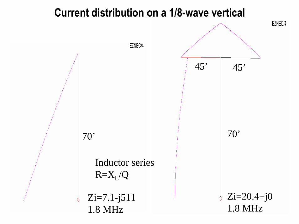
Short Vertical Rr
C Versus L Loading

Advantages Of Capacitive Loading
• Produces higher Rr
• Very efficient
• Can usually be integrated into the support structure.

PRACTICAL MATTERS
When I erect a short vertical I do the following:
If possible, I use enough capacitive top loading to resonate the antenna a little bit above the top of the band.

PRACTICAL MATTERS
I then install a small inductor at the base to perform the following functions:
• Resonate the antenna to the desired frequency and provide matching.
• Usually this inductor will be small enough to have very little effect on efficiency.

PRACTICAL MATTERS
Matching can be done by using the
inductor as part of the matching
network and/or,
the inductor can be tapped and a
relay used to vary the center
frequency of the antenna to allow
movement across the band.

ANOTHER USEFUL TRICK
Add enough top-loading so that the antenna is resonant below the band.
This means that:
the input impedance will be inductive,
the resistive part of the input impedance will be larger and
you can resonate the antenna with a simple and efficient series capacitor at the input.

ANOTHER USEFUL TRICK
In addition:If you vary this capacitor you can tune the antenna across the band.
This is similar in concept to the hairpin match used in Yagies except that now you make the element a bit longer.
Sometimes this is called a “C”match.

80 m “T” vertical

Top Loading Examples

Top loading with guys

Optimum umbrellas

SLOPING TOP WIRES
• You can use two or more sloping top loading wires.
• The closer the angle to 90 degrees the better.
• The more wires you use the greater the loading but as you add more wires the additional improvement gets smaller.

SLOPING TOP WIRES
• Usually four wires are plenty.
• Adding a skirt wire to a given number of sloping wires gives about the same maximum Rr but with shorter wires.

Loaded wire vertical

80 m example
As you go away fromThe current loop (maximum)The impedance rises.
As you “over-load” the antennaThe feedpoint impedance alsoRises and becomes inductive.You can then tune with a capacitor.

Shunt feed
feedpoint
Gamma match

Shunt-feed example
Metal roof160 m

Multiple vertical wires.
feedpoint
Down leads arrangedSymmetrically. If notthen the currents won’t share.

Advantages of Multiple Wires
• One of the problems with short loaded
wire antennas is conductor loss.
• Multiple wires can lower conductor loss.

Advantages of Multiple Wires
• They may provide a wider match bandwidth.
• Larger diameter conductors or better yet, multiple spaced conductors, will have less reactance and the reactance changes more slowly with frequency.

Advantages of Multiple Wires
• The feedpoint impedance when feeding one of the wires will increase by the square of the number of wires i.e. for three wires, the feedpoint impedance will be nine times that for a single wire.
• Multiple spaced top-hat wires increase the loading effect.

Another trick for improving bandwidth
Zi = 50 Ohm @ 1.830 MHz
130’
50’
This antenna was resonantbelow the band, so I used a series C to resonate

Inductive Loading

Efficiency And Coil Position

Combining Capacitive and Inductive Loading
• You can combine both capacitive top loading and inductive loading.
• You would normally do this when it is not possible to erect sufficient top loading to reach resonance.
• With no top loading and given coil Q, the optimum coil location will be near the center.

Combining Capacitive and Inductive Loading
• As top loading is added, the optimum inductor location moves up towards the top.
• However! With added top loading the effect of inductor location becomes much less critical and in fact for very much top loading it is more convenient to locate the inductor at the base.
• This cost little in efficiency.

Tactics For High Efficiency• Maximize Rr:
– taller element– Capacitive end loading– move loading L up into the vertical
• Minimize Rloss:– Minimize conductor, loading coil and matching
resistances– i.e. larger conductors, multiple conductors,
higher Q inductors, etc– Minimize ground loss

Ground Currents

E and H fields around a vertical
ground
soil equivalent
Ih

H field and induced currents• Current will be induced in the soil at right angles to the H-field.• If a conductor is at right angels to the H-field then the maximum
current will be induced in it. But if the conductor is parallel to the field then no current will be induced.
H
Iradial
radial
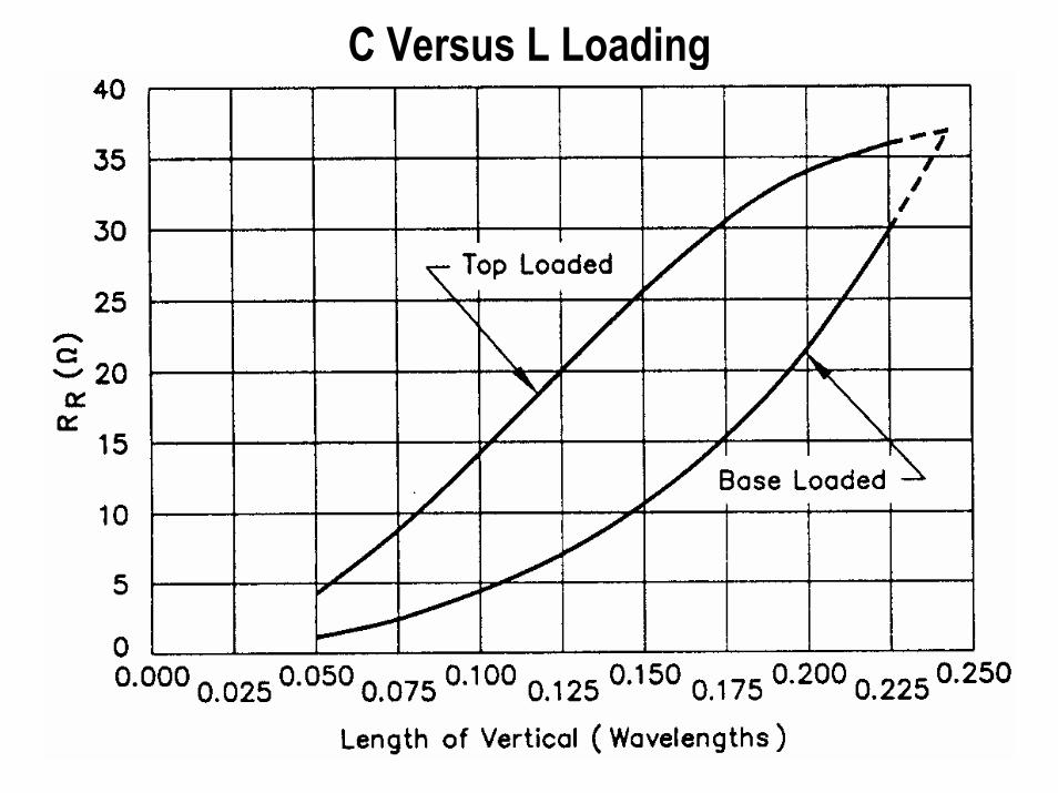
GROUND LOSSES
• The H-field will introduce horizontal ground currents.
• The E-field will introduce vertical ground currents.
• These losses are I2R in nature, i.e. they vary as the square of the H and E-field intensities.

GROUND LOSSES
• The ground losses for a given antenna are highly dependent on the electrical characteristics of the soil within a half-wavelength of the antenna horizontally and one skin depth vertically.
• The soil characteristics vary with frequency at HF.
• The function of the ground system is to reduce these losses to an acceptable limit.

Fundamental Limitation
The ground system around the antenna
does nothing for the far-field pattern
except to increase the power radiated for
a given input power.

ARRAY GROUND SYSTEMS
• In a single element vertical, the radial wire ground system is by nature optimum in relation to the H-field orientation.
• In a multi-element vertical array if each element has its own radial system then radial wires are fine.

ARRAY GROUND SYSTEMS
• However, if the radials are abbreviated so that they do not overlap as is standard practice, then in some areas the ground wires will not be optimally aligned and the ground losses will be higher.
• This can be overcome by using a grid ground system over at least part of the area near the antennas.

Soil Characteristics

Ground Parameters• Soil is characterized by it's conductivity
and permittivity.
– the resistance of the soil for current flowing through it is inversely proportional to it's conductivity with units of Siemens/meter (S/m).
– higher conductivity means lower ground loss.

Ground Parameters
– the permittivity (dielectric constant) is related to the reactance of the soil for current flowing in it.
– permitivity has units of Farads/meter.
– we usually talk about the relativedielectric constant, Er, which is 1 for air.

Typical Ground Characteristicsseawater = 5000 mS/m

Comment on Soil Charts
• The typical soils listed in tables are for general guidance only.
• Most of the information is for BC frequencies and conductivity only.
• Your soil will almost certainly be different.

Comment on Soil Charts• The soil parameters will vary both
horizontally and vertically
• The soil parameters will also vary during the year depending on temperature, rainfall, etc.
• The best way to estimate your soil parameters is to directly measure them.
See QEX Nov/Dec 2006

N6LF Ground Conductivity
0.01
0.012
0.014
0.016
0.018
0.02
0.022
0.024
0.026
0.028
1 2 3 4 5 6 7 8 9 10
Frequency (MHz)
Soil
cond
uctiv
ity (S
/m)
03-28-04 soil test data
trendline
data

N6LF Ground Permitivity
40
45
50
55
60
65
70
75
80
85
1 2 3 4 5 6 7 8 9 10
Frequency (MHz)
Rel
ativ
e di
elec
tric
con
stan
t
03-28-04 soil test data
datatrendline

Skin depth equations• Skin depth in an arbitrary material is given by:
• Where:• δ = skin or penetration depth• ω = 2πf, f = frequency• σ= conductivity [Siemens/meter, S/m]• μ = μr μo=permeability• μo= permeability of vacuum = 4π10-7 [Henry/meter]• μr = relative permeability• ε =εr εo = permittivity• εo = permittivity of vacuum = 8.854x10⁻¹² [Farad/meter]• εr = relative permittivity
1/ 222 1 1 (1)σδ
ωεω με
−
⎡ ⎤⎛ ⎞ ⎛ ⎞⎢ ⎥= + −⎜ ⎟ ⎜ ⎟⎝ ⎠⎢ ⎥⎝ ⎠ ⎣ ⎦

Penetration Depth In Soil

Wavelength in free space
MHz
wavelength in free space299.79 [ ]
c = speed of light 299.79E6 m/s f = frequency
f = frequency in MHz
o
o
MHz
c mf f
λ
λ
=
= =

Wavelength in soil• The wavelength in soil (λ) will depend on σ
and εr:
1/ 42
2
o
r
o
λλσεωε
=⎡ ⎤⎛ ⎞
+⎢ ⎥⎜ ⎟⎝ ⎠⎣ ⎦

Wavelength in soil
0.1
1
10
100
1000
0.1 1 10 100
Frequency (MHz)
Wav
elen
gth
In S
oil
(m)
seawater 5/81
fresh water .001/80
poor .001/5
average .005/13
very good .03/20

Ground Systems For Verticals

Choices for ground systems• There are three categories of ground systems:
– Elevated radials– Radials lying close to the ground surface– Buried radials
• Each of these behaves differently!

Radial currents
Free spaceResonant radials

Radial currents at three different heights
Free space
1” above average ground
12” below ground

Measured radial currentsArch Doty Measurements 160 m

H-Field Currents Near A Vertical
Iz = zone currentInduced by H-field

Iz, zone current
0
1
2
3
0 0.1 0.2 0.3 0.4 0.5 0.6 0.7 0.8 0.9 1
r (distance from base in wavelengths)
Iz (A
) , z
one
curr
ent i
n gr
oud
constant radiated power =37 W
h=.1
h=.15
h=.2
h=.25
h=.3
h=.4 h=.5
Remember! Losses are proportional to I2

H-Field Loss
0
10
20
30
40
50
60
70
80
90
100
0.00 0.05 0.10 0.15 0.20 0.25 0.30 0.35 0.40 0.45 0.50
r (wavelengths)
Tota
l H-fi
eld
grou
nd lo
ss w
ithin
r (W
) h=0.1
h=0.15
h=0.20
h=0.25
h=0.30
h=0.40
h=0.50
0.005/13 ground, 1.8 MHz, Pr=37 W

Electric Field Intensity Near The Base• f = 1.8 MHz and Power = 1500 W

E-Field Loss
0.10
1.00
10.00
100.00
0.00 0.05 0.10 0.15 0.20 0.25 0.30 0.35 0.40 0.45 0.50
r (wavelengths)
tota
l E-fi
eld
grou
nd lo
ss (W
) with
in r
h=0.10
h=0.15
h=0.20
h=0.40
h=0.30
h=0.25 Pr=37W, f=1.83 MHz, sigma = 0.005 S/m

Rg With A Perfect Ground Screen
0.1
1.0
10.0
100.0
0.00 0.05 0.10 0.15 0.20 0.25 0.30 0.35 0.40 0.45 0.50
Ground-screen radius (wavelengths)
Rg
(Ohm
s)
f=1.8 MHz, average groundincludes H & E-field Pg
h=0.10
h=0.40
h=0.30
h=0.25h=0.15
h=0.20
Rg = Ploss/I2

Variable Rg with h???
• What’s going on here.
• The conventional wisdom is that a given ground system, over a given soil, at a given frequency, will have some equivalent Rg independent of the antenna.
• This isn’t true!

Variable Rg with h???
• Rg represents the equivalent series resistance component of the input impedance that accounts for the ground loss (Pg) for a given excitation current.
• As we reduce the height of the antenna, Rr goes down, so for the same power we have to jack up the current which increases the fields around the base.

Variable Rg with h???
• But the losses go as I2!
• Yes, the ground loss does increase but the value for Rg actually goes down a bit.

CLASSICAL 120 RADIAL GROUND SCREEN
Radials about .4 λ long
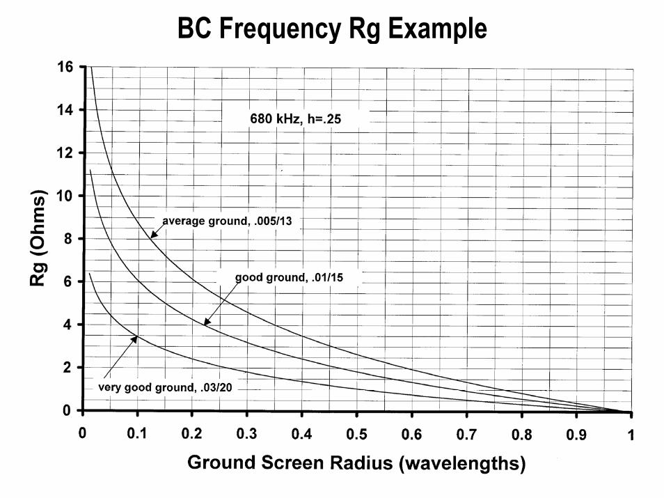
BC Frequency Rg Example

Optimum Ground Wire Usage
0
5
10
15
20
25
30
0 0.1 0.2 0.3 0.4 0.5 0.6 0.7 0.8 0.9 1
Ground radial Radius (wavelengths)
Rg
(Ohm
s)
N=8
N=16
N=32
N=64
N=128
N=256perfect screen
f=1.8 MHz, average ground, .005/13, h=0.25

Current In Radials

Ground Current And Radials
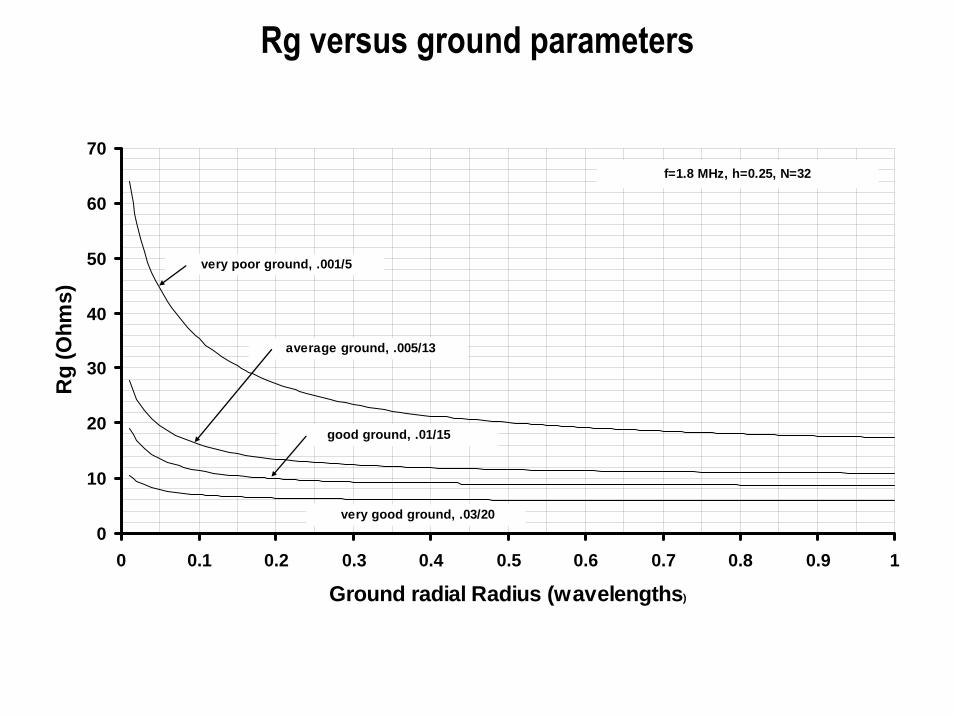
Rg versus ground parameters
0
10
20
30
40
50
60
70
0 0.1 0.2 0.3 0.4 0.5 0.6 0.7 0.8 0.9 1
Ground radial Radius (wavelengths)
Rg
(Ohm
s)
f=1.8 MHz, h=0.25, N=32
average ground, .005/13
very poor ground, .001/5
good ground, .01/15
very good ground, .03/20

Efficiency versus radial number
-3.5
-3
-2.5
-2
-1.5
-1
-0.5
0
0 10 20 30 40 50 60
Number of radials
Effic
ienc
y (d
B)
average ground, .005/13
very poor ground, .001/5
good ground, .01/15
very good ground, .03/20
f=1.8 MHz, h=0.25, radial length =0.25
Assuming Rr = 36 Ohms

Rg For h=0.1 Wavelength
0.0
0.5
1.0
1.5
2.0
2.5
3.0
3.5
4.0
4.5
5.0
5.5
6.0
0.00 0.05 0.10 0.15 0.20 0.25 0.30 0.35 0.40 0.45 0.50
radial length (wavelengths)
Rg
(Ohm
s)
h=0.1, f=1.8 MHz,gnd=13/.005
N=16
perfect screen
N=32
N=64
N=128
N=256
N=512

Series base resistance (Rs)
35
40
45
50
55
60
65
70
1.80E+06 1.82E+06 1.84E+06 1.86E+06 1.88E+06 1.90E+06 1.92E+06 1.94E+06 1.96E+06 1.98E+06 2.00E+06
Frequency (Hz)
Rs
(Ohm
)
4 radials
8 radials
16 radials
32 radials
64 radials
160 m test verticalAugust 2006
run 2

Rs versus radial number
40
45
50
55
60
65
4 14 24 34 44 54 64
number of radials
Rs
(Ohm
)
160 m test verticalAugust 2006
run 21.9 MHz

Series base input reactance (Xs)
-50
-40
-30
-20
-10
0
10
20
30
40
50
1.80E+06 1.82E+06 1.84E+06 1.86E+06 1.88E+06 1.90E+06 1.92E+06 1.94E+06 1.96E+06 1.98E+06 2.00E+06
Frequency (Hz)
Xs (O
hm)
160 m test verticalFr = 1.9 MHzAugust 2006
run 2
4 radials64 radials

Field strength versus radial number
0
0.5
1
1.5
2
2.5
0 10 20 30 40 50 60 70
Number of radials
chan
ge in
fiel
d st
reng
th (d
B)
160 m test verticalAugust 2006
run 2

Calculated change in field strength
0
0.2
0.4
0.6
0.8
1
1.2
0 10 20 30 40 50 60 70
Number of radials
Effic
ienc
y in
crea
se (d
B)
f=1.8 MHz, h=0.25, radial length =0.25
average ground, .005/13
very poor ground, .001/5
good ground, .01/15
very good ground, .03/20

Rs versus radial number and frequency
30
35
40
45
50
55
60
65
70
75
80
6.9 6.95 7 7.05 7.1 7.15 7.2 7.25 7.3
Frequency (MHz)
Rs
(Ohm
s)
Rs40 m vertical test, 4-06-07
4 radials
8 radials
16 radials
32 radials
0 radialsground post only

Change in Rs with radial number
30.00
35.00
40.00
45.00
50.00
55.00
60.00
65.00
70.00
75.00
0 5 10 15 20 25 30 35
Number of radials
Rs
(Ohm
s)
Rs40 m vertical test, 4-06-07
6.9 MHz
7.3 MHz
7.1 MHz7.2 MHz
7.0 MHz

Xs versus radial number and frequency
-20
-10
0
10
20
30
40
6.9 6.95 7 7.05 7.1 7.15 7.2 7.25 7.3
Frequency (MHz)
Xs (O
hms)
Xs40 m vertical test, 4-06-07
4 radials
8 radials
16 radials
32 radials
0 radialsground post only

Resonant frequency shift
6.8
6.85
6.9
6.95
7
7.05
7.1
7.15
7.2
0 5 10 15 20 25 30 35
Number of radials
Res
onan
t fre
quen
cy (M
Hz)
resoant frequency40 m vertical test, 4-06-07

Relative gain versus radial number
0
0.5
1
1.5
2
2.5
3
0 5 10 15 20 25 30 35
Number of radials
Rel
ativ
e ga
in (d
B)
relative transmission gain40 m vertical test, 4-06-07
7.3 MHz
7.1 MHz7.2 MHz
7.0 MHz

Wire grid ground systems
Zs = impedance of the soilZg = impedance of the grid or ground screen
IT = total current returning to the antenna

Free space impedance• What do we mean by the soil impedance? We know that the
impedance of free space is the ratio of the E-field to the H-field components in an E-M wave and is given by:
•
• Where:• μo = permeability of free space = 4π 10-7• εo = permittivity of free space = 8.854 x 10⁻¹²
Ohm 7.376==o
ospaceZ
εμ

Soil impedance• We can extend this concept to soil by taking into account the
conductivity and permittivity:
•• Where:• εr = relative permittivity• σ = soil conductivity in S/m• ω = 2 π f, where f is the frequency in Hz.• Note that Zs can be complex.
⎟⎟⎠
⎞⎜⎜⎝
⎛−
=
⎥⎥⎥⎥⎥
⎦
⎤
⎢⎢⎢⎢⎢
⎣
⎡
⎟⎟⎠
⎞⎜⎜⎝
⎛−
=
or
or
o
os
jj
Z
ωεσε
ωεσε
εμ 7.3761

Ground impedance (Zg)
1.0
10.0
100.0
1000.0
0.1 1 10 100
Frequency (MHz)
|Zg|
(Ohm
s)
salt water5/81
fresh water.001/80
.001/3
.001/5
.002/13
.005/13 .03/20
Ground impedance
Note: this is for constant parameters with frequency!

Impedance of a grid• We can also state the equivalent impedance for the grid:
• Where:• d = spacing of grid wires in meters• a = radius of grid wires in meters• Note: this equation looks very much like that for a two wire
transmission line!
⎟⎠⎞
⎜⎝⎛=
addjfZ og π
μ2
ln

Typical grid calculation• Let's see what Zs is for average ground at 1.83 MHz.• Plugging εr = 15 and σ = 0.005 S/m into the equation for
Zs: Zs = 42.2+j31.28 Ohms, |Zs| = 52.6 Ohms.
• If the ground screen is made with #12 wire spaced 24", Zg = j6.41 Ohms and |Zg| = 6.41 Ohms.
TTsg
gs II
ZZ
ZI 113.0=
+=

Grid calculation• Loss is proportional to I squared!
• We see that for this ground characteristic and frequency, 24" spacing in the grid reduces the ground loss to about 1% of what it would have been without the screen.

Radial system impedance (Zr)
1
10
100
1000
10000
0 0.05 0.1 0.15 0.2 0.25 0.3 0.35 0.4 0.45 0.5
Distance from base (WL)
|Zr|
(Ohm
s)
N=4
N=8
N=16
N=32
N=64
N=128
f=1.8 MHz, #12 wire
N=256
N=512
50 Ohms

Ground-Plane Antenna
λ/4
λ/4
λ/4
λ/4
λ/4
isolation choke/balun

Feedpoint Impedance

Sloping Radials
45 degree sloping radials

Effect Of Radial Length On Gain

COMMENT• The electrical length for a resonant λ/4
radial will depend on the height above ground.
• Radials very close to or actually lying on the ground will have to be much shorter than the free space length to be resonant.
• For radials near ground the high loss notch appears at much shorter lengths.

COMMENT
• The high loss notch becomes much less pronounced as the number of radials is increased and the ground characteristics are improved.
• Buried radials can show the same problem in poor soil when there are only a small number of radials.

PROBLEMS WITH NON-IDENTICAL RADIALS
• Unequal radial currents leading to asymmetrical radiation patterns
• Varying reactive and resistive components of the input impedance
• Increased ground loss

Some Advice on Elevated Radials
• Make all the radials as uniform as possible; same length, height over ground, wire size, tension (amount of droop) and maintain symmetry.
• Keep the radials away from other conductors fences, buildings or other antennas.

Some Advice on Elevated Radials
• Use as many radials as possible
• Place radials as high above ground as practical
• Make the radial lengths a bit longer or shorter than 1/4 wave
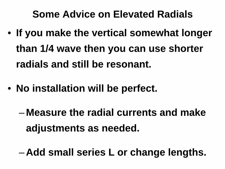
Some Advice on Elevated Radials
• If you make the vertical somewhat longer than 1/4 wave then you can use shorter radials and still be resonant.
• No installation will be perfect.
– Measure the radial currents and make adjustments as needed.
– Add small series L or change lengths.

ALTERNATE RADIAL SYSTEMS
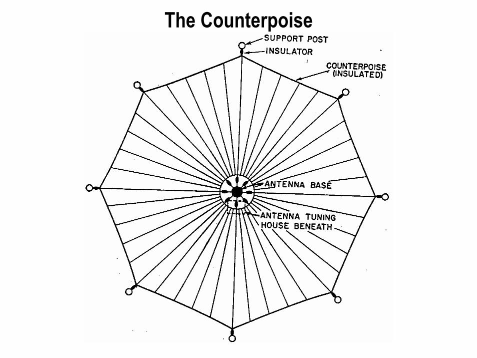
The Counterpoise

DECOUPLING CHOKES