For Peer Review Keywords - Home - Anil V. Rao's Website |vdol.mae.ufl.edu/.../F-1-Optimal-Control-Energy-Recovery.pdfFor Peer Review Optimal control of Formula One car energy recovery

For Peer ReviewOptimal control of Formula One car energy

recovery systems

D. J. N. Limebeer, G. Perantoni and A. V. Rao ∗

November 8, 2013

Abstract

The utility of orthogonal collocation methods in the solution of opti-mal control problems relating to Formula One racing is demonstrated.These methods can be used to optimise driver controls such as thesteering, braking and throttle usage, and the optimisation of vehicleparameters such as aerodynamic down force distributions. Of partic-ular interest is the optimal usage of energy recovery systems. Con-temporary kinetic energy recovery systems (KERS) are studied andcompared with future hybrid kinetic-thermal energy recovery systemsknown as (ERS-K) and (ERS-H). It is demonstrated that these sys-tems, when properly controlled, can produce contemporary lap timeusing approximately two thirds of the fuel required by present-dayvehicles.

Keywords: numerical optimal control; orthogonal collocation; pseu-dospectral methods; lap-time simulation; Formula One car modelling; energyrecovery systems.

1 Introduction

Minimum-lap-time optimal control problems for Formula One cars arenot easy to solve. A discussion of some of the technical difficulties

∗David J. N. Limebeer (Corresponding Author) ([email protected]) and Gi-acomo Perantoni ([email protected]) are with the Department of Engineer-ing Science, University of Oxford, Parks Road, Oxford, OX1 3PJ. Anil V. Rao ([email protected]) is with the Department of Mechanical and Aerospace Engineering, Uni-versity of Florida, Gainesville, FL 32611-6250. The work was supported by the UK Engi-neering and Physical Sciences Research Council.

Page 1 of 40

http://mc.manuscriptcentral.com/tcon

International Journal of Control

123456789101112131415161718192021222324252627282930313233343536373839404142434445464748495051525354555657585960

For Peer Review

related to the solution of these problems can be found in existing literature;see for example [1, 2]. A historical overview of some of the optimal controlliterature relating to vehicular applications can be found in [3].

A reader familiar with the classical theory of optimal control and thecalculus of variations might think that the most natural approach to thesolution of these problems is to use first-order necessary conditions to for-mulate and solve a two-point-boundary-value problem. This is the approachtaken in [4], where two motorcycle manoeuvring problems are solved. In laterdevelopments of this line of research an indirect method is used to examineminimum time manoeuvres for a single-track car model through a U-turn [5].

In some recent work a direct transcription method is used to solve vari-ous minimum-lap-time optimal control problems for a complete lap [6]. Thiswork employed a car model that reproduces the longitudinal, lateral and yawdynamics of the vehicle, a realistic tyre model and a curvilinear (differentialgeometric) description of the track. This approach was successful in solv-ing several minimum-lap-time optimal-control problems with a number ofcontrol and parameter optimisation variations. The Modelica modelling andoptimization environment [7] has also been used to solve minimum lap timeproblems [8].

Much of the more recent work in this area is directed to improving thesolubility of these problems and focusses on simplifying the vehicle and tyremodels, and widening the use of linear optimal control techniques. These in-clude the use of quasi-steady-state models [9] and the use of linear quadraticpreview and model predictive control. One approach to minimising the bur-den associated with minimum-lap-time studies is the use of linear quadratic(LQ) preview to follow a prescribed driving line at a fixed speed [10]. Themethod proposed makes use of multiple linear models and a gain schedul-ing scheme, with its operation demonstrated on three track segments. Ideasbased on linear approximations have been developed in [11, 12], where (lin-ear time-varying) model predictive control (MP) rather than linear previewcontrol is exploited. This approximation allows one to define the problem offinding a sub-optimal racing line and a speed profile as a convex optimisationproblem.

In this paper we study the use of a direct orthogonal collocation methodfor solving racing-related optimal control problems. Apart from the use of adifferent optimal control methodology (as compared with [6]), the car modelhas been upgraded to use a more realistic aerodynamic model. A key focus ofthis paper is the optimal control of the energy recovery systems. Under the2013 Formula One technical regulations a Kinetic Energy Recovery System(KERS) is allowed to recover kinetic energy from the car during braking,store that energy and then make it available to propel the car at some later

2

Page 2 of 40



123456789101112131415161718192021222324252627282930313233343536373839404142434445464748495051525354555657585960

For Peer Review

point in the race. The energy drawn from the energy store to propel the caris limited to 400 KJ on a per-lap basis [13].

In the lead up to the 2008-2017 Formula One engine development freeze itwas estimated that an average of 4 milliseconds per lap were gained for everymillion dollars spent on engine development [14]. This indicates that furtherengine development is bound not only to be prohibitively expensive, butalso incremental in terms of future technical progress. In order to improveFormula One’s ‘green’ credentials, and accelerate road-car relevant powertrain developments, it was decided that from 2014 Formula One cars willhave to recover thermal as well as kinetic energy that would otherwise belost [15]. The hope is that the introduction of hybrid thermal-kinetic energyrecovery systems will produce gains that are far more significant and cost-effective than engine development alone. The results of this paper show thatcontemporary lap times can be achieved using less powerful turbo-chargedengines, which require only two-thirds of the fuel required by contemporarycars, when thermal and kinetic energy recovery systems are employed.

The vehicle and track models are covered in Section 2. Most of thismaterial is standard, or has appeared elsewhere and so this treatment iscorrespondingly brief. The tyre modelling is covered in Appendix A withthe vehicle parameters given in Appendix B. Section 3 briefly reviews themathematical background underpinning orthogonal collocation transcriptiontechniques. Key is the classical theory of orthogonal polynomials, whichunderpins most numerical integration schemes — particularly integrationquadratures. The results appear in Section 4. The performance of the nomi-nal car is studied first, with this preliminary investigation used as a vehiclefor illustrating the use and features of adaptive pseudospectral optimizationtechniques. The main results of the paper relate to the optimal control ofenergy storage systems in Formula One racing. We begin with the opti-mal control of contemporary kinetic energy recovery systems, which is thenfollowed by an investigation of the hybrid kinetic-thermal energy recoverysystem to be introduced in 2014. The conclusions and acknowledgementsappear in Sections 5 and 6.

2 Car and Track Model

The track and car kinematics are modelled using ideas from classical differ-ential geometry. As was explained in [6], the track description is based onmeasured data with the curvature of the track found as the solution of asubsidiary optimal control problem. The car model is standard and is basedon a rigid-body representation of a chassis with longitudinal, lateral and

3

Page 3 of 40



123456789101112131415161718192021222324252627282930313233343536373839404142434445464748495051525354555657585960

For Peer Review

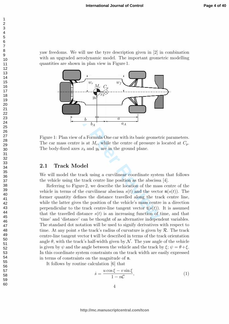
yaw freedoms. We will use the tyre description given in [2] in combinationwith an upgraded aerodynamic model. The important geometric modellingquantities are shown in plan view in Figure 1.

Mc Cpwfwr

b abA aA

xbyb

Figure 1: Plan view of a Formula One car with its basic geometric parameters.The car mass centre is at Mc, while the centre of pressure is located at Cp.The body-fixed axes xb and yb are in the ground plane.

2.1 Track Model

We will model the track using a curvilinear coordinate system that followsthe vehicle using the track centre line position as the abscissa [4].

Referring to Figure 2, we describe the location of the mass centre of thevehicle in terms of the curvilinear abscissa s(t) and the vector n(s(t)). Theformer quantity defines the distance travelled along the track centre line,while the latter gives the position of the vehicle’s mass centre in a directionperpendicular to the track centre-line tangent vector t(s(t)). It is assumedthat the travelled distance s(t) is an increasing function of time, and that‘time’ and ‘distance’ can be thought of as alternative independent variables.The standard dot notation will be used to signify derivatives with respect totime. At any point s the track’s radius of curvature is given by R. The trackcentre-line tangent vector t will be described in terms of the track orientationangle θ, with the track’s half-width given by N . The yaw angle of the vehicleis given by ψ and the angle between the vehicle and the track by ξ; ψ = θ+ξ.In this coordinate system constraints on the track width are easily expressedin terms of constraints on the magnitude of n.

It follows by routine calculation [6] that

s =u cos ξ − v sin ξ

1− nC , (1)

4

Page 4 of 40



123456789101112131415161718192021222324252627282930313233343536373839404142434445464748495051525354555657585960

For Peer Reviews

ZNR

θ

nx

ny n t

ψξ

Figure 2: Curvilinear-coordinate-based description of a track segment Z.The independent variable s represents the elapsed centre-line distance trav-elled, with R(s) the radius of curvature and N (s) the track half-width; nxand ny represent an inertial reference frame.

in which u and v are the longitudinal and lateral components of the car’svelocity. The rate of change of n is given by

n = u sin ξ + v cos ξ. (2)

Differentiating ψ = ξ + θ with respect to time results in

ξ = ψ − Cs. (3)

2.1.1 Change of Independent Variable

The ‘distance travelled’ will be used as the independent variable. This hasthe advantage of maintaining an explicit connection with the track position,as well as reducing (by one) the number of problem state variables. Suppose

dt =dt

dsds = Sf (s)ds,

where Sf comes from (1) as follows

Sf =

(ds

dt

)−1

=1− nC

u cos ξ − v sin ξ. (4)

5

Page 5 of 40



123456789101112131415161718192021222324252627282930313233343536373839404142434445464748495051525354555657585960

For Peer Review

The quantity Sf is the reciprocal of the component of the vehicle velocity inthe track-tangent direction (on the centre line at s). There follows

dn

ds= Sf (u sin ξ + v cos ξ) (5)

from (2), anddξ

ds= Sfω − C (6)

from (3); ω = ψ is the vehicle yaw rate.

2.2 Car Model

Each tyre produces longitudinal and lateral forces that are responsive to thetyres’ slip; see Appendix A. These forces together with the steer and yawangle definitions are given in Figure 3.

nx

ny

uv

ψ

δ

δ

FrlxFrly

FrrxFrry

FflxFfly

FfrxFfry

Figure 3: Tyre force system. The inertial reference frame is shown as nx andny.

Balancing forces in the longitudinal and lateral directions, while also bal-

6

Page 6 of 40



123456789101112131415161718192021222324252627282930313233343536373839404142434445464748495051525354555657585960

For Peer Review

ancing the yaw moments, gives

Md

dtu(t) = Mωv + Fx

Md

dtv(t) = −Mωu+ Fy

Izd

dtω(t) = a (cos δ(Ffr y + Ffl y) + sin δ(Ffr x + Ffl x)) +

wf (sin δFfr y − cos δFfr x)− wrFrr x +

wf (cos δFfl x − sin δFfl y) + wrFrl x − b (Frr y + Frl y) , (7)

in which Fx and Fy are the longitudinal and lateral forces, respectively, actingon the car. These forces are given by

Fx = cos δ(Ffrx + Fflx)− sin δ(Ffry + Ffly) + (Frrx + Frlx) + Fax (8)

Fy = cos δ(Ffry + Ffly) + sin δ(Ffrx + Fflx) + (Frry + Frly) (9)

in which Fax is the aerodynamic drag force. These equations can be expressedin terms of the independent variable s as follows:

du

ds= Sf (s)u (10)

dv

ds= Sf (s)v (11)

dω

ds= Sf (s)ω. (12)

2.3 Tyre Forces

The tyre forces have normal, longitudinal and lateral components that acton the vehicle’s chassis at the tyre-ground contact points and react on theinertial frame. The rear-wheel tyre forces are expressed in the vehicle’s body-fixed reference frame, while the front tyre forces are expressed in a steeredreference frame; refer again to Figure 3. In each case these forces are afunction of the normal load and the tyre’s longitudinal and lateral slip.

2.3.1 Load Transfer

In order to compute the time-varying tyre loads normal to the ground plane,we balance the forces acting on the car in the nz direction and balance mo-ments around the body-fixed xb- and yb-axes; see Figure 1. Balancing thevertical forces gives

0 = Frrz + Frlz + Ffrz + Fflz +Mg + Faz, (13)

7

Page 7 of 40



123456789101112131415161718192021222324252627282930313233343536373839404142434445464748495051525354555657585960

For Peer Review

in which the F··z’s are the vertical tyre forces for each of its four wheels, g isthe acceleration due to gravity and Faz is the aerodynamic down force actingon the car. Balancing moments around the car’s body-fixed xb-axis gives

0 = wr(Frlz − Frrz) + wf (Fflz − Ffrz) + hFy, (14)

in which Fy is the lateral inertial force acting on the car’s mass centre; see(9). Balancing moments around the car’s body-fixed yb-axis gives

0 = b(Frrz + Frlz)− a(Ffrz + Fflz) + hFx + (aA − a)Faz, (15)

where Fx is the longitudinal inertial force acting on the car’s mass centre (see (8)), while Faz is the aerodynamic down force.

Equations (13), (14) and (15) are a set of linear equations in four un-knowns. A unique solution for the tyre loads can be obtained by adding asuspension-related roll balance relationship, in which the lateral load differ-ence across the front axle is some fraction of the whole

Ffrz − Fflz = D(Ffrz + Frrz − Fflz − Frlz), (16)

where D ∈ [0, 1].

2.3.2 Non-Negative Tyre Loads

The forces satisfying equations (13), (14), (15) and (16) are potentially bothpositive and negative. Negative forces are indicative of vertical reactionforces, while positive forces are fictitious ‘forces of attraction’. Since themodel being used here has no pitch, roll or heave freedoms, none of thewheels is free to leave the road, while also keeping faith with (13) to (16).

To cater for the possible ‘positive force’ situation within a nonlinear pro-gramming environment we introduce the vector

Fz =

FfrzFflzFrrzFrlz

, (17)

and define a vector of non-positive loads

Fz = min(Fz, 0); (18)

the minimum function min(·, ·) is interpreted element-wise. It is clear thatFz and Fz will be equal unless at least one entry of Fz is positive (i.e. non-physical). We now argue that the model must respect the laws of mechanics

8

Page 8 of 40



123456789101112131415161718192021222324252627282930313233343536373839404142434445464748495051525354555657585960

For Peer Review

at all times and so equations (13), (14) and (15) must be enforced uncondi-tionally. In contrast, we assume that the solution to (16), which is only anapproximate representation of the suspension system, can be ‘relaxed’ in theevent of a wheel load sign reversal.

Equations (13), (14) and (15) can be written in matrix form as

A1Fz = c, (19)

while (16) is given byA2Fz = 0. (20)

In order to deal with the ‘light wheel’ situation, we combine (19) and (20)[A1 00 A2

] [FzFz

]=

[c0

], (21)

in which Fz in (20) has been replaced by Fz. In the situation where allthe wheels are normally loaded, Fz = Fz and (21) reduces to (13), (14),(15) and (16). On the other hand, if there is a ‘light wheel’, the mechanicsequations (13), (14) and (15) will be satisfied by the non-positive forces Fz,while the roll balance equation is satisfied by the now fictitious forces Fzthat contain a force of attraction. The non-positive forces Fz are used torepresent the normal tyre loads in the rest of the model. It is clear thatthe four components of Fz have to satisfy the nonlinear circularly-dependentrelationship (21), which will be solved by a NLP algorithm.

2.4 Aerodynamic Loads

The external forces acting on the car come from the tyres and from aerody-namic influences. The aerodynamic force is applied at the centre of pressure,which is located in the vehicle’s plane of symmetry. The drag and lift forcesare given by

Fax = −0.5CD(u) ρAu2, (22)

andFaz = 0.5CL(u) ρAu2, (23)

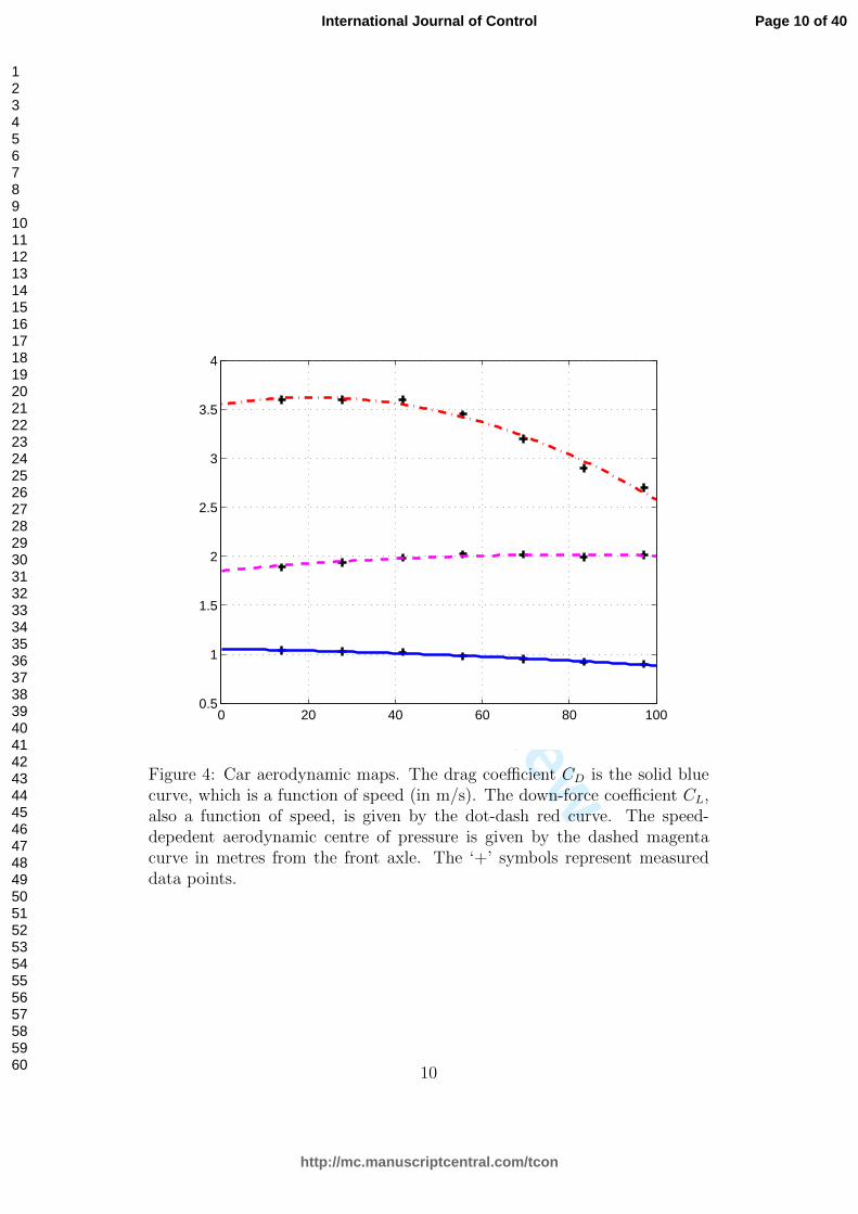
respectively. The speed-dependent drag and down-force coefficients, and thespeed-dependent location of the aerodynamic centre of pressure are given inFigure 4.

9

Page 9 of 40



123456789101112131415161718192021222324252627282930313233343536373839404142434445464748495051525354555657585960

For Peer Review

0 20 40 60 80 1000.5

1

1.5

2

2.5

3

3.5

4

Figure 4: Car aerodynamic maps. The drag coefficient CD is the solid bluecurve, which is a function of speed (in m/s). The down-force coefficient CL,also a function of speed, is given by the dot-dash red curve. The speed-depedent aerodynamic centre of pressure is given by the dashed magentacurve in metres from the front axle. The ‘+’ symbols represent measureddata points.

10

Page 10 of 40



123456789101112131415161718192021222324252627282930313233343536373839404142434445464748495051525354555657585960

For Peer Review

2.5 Wheel Torque Distribution

In order to optimise the vehicle’s performance, one needs to control thetorques applied to the individual road wheels. The braking system appliesequal pressure to the brake callipers on each axle, with the braking pressuresbetween the front and rear axles satisfying a design ratio. The drive torquesapplied to the rear wheels are controlled by a differential mechanism.

2.5.1 Brakes

We approximate equal brake calliper pressures with equal braking torqueswhen neither wheel on a particular axle is locked. If a wheel ‘locks up’, thebraking torque applied to the locked wheel may be lower than that applied tothe rolling wheel. For the front wheels this constraint is modelled as follows

0 = max(ωfr, 0) max(ωfl, 0)(Ffrx − Fflx), (24)

in which ωfr and ωfl are the angular velocities of the front right and frontleft wheel, respectively. If either road wheel ‘locks up’, the correspondingangular velocity will be non-positive and the braking torque constraint (24)will be inactive.

2.5.2 Differential

The drive torque is delivered to the rear wheels through a limited-slip differ-ential, which is modelled by

R(Flrx − Frrx) = −kd(ωlr − ωrr), (25)

in which ωlr and ωrr are the rear-wheel angular velocities, R is the wheelradius and kd is a torsional damping coefficient. The special cases of anopen- and a locked-differential correspond to kd = 0 and kd arbitrarily largerespectively. Limited slipping occurs between these extremes.

3 Orthogonal Collation Methods

The use of orthogonal collocation (pseudospectral) methods in trajectoryoptimisation problems has been gathering pace since the 1980’s. An earlyexample was the solution of the classical brachistochrone problem using aChebyshev polynomial expansion description of the state and control [16]. Inthese techniques a series of node points, called collocation points, are definedat which the state and control vectors are represented in discrete form. In

11

Page 11 of 40



123456789101112131415161718192021222324252627282930313233343536373839404142434445464748495051525354555657585960

For Peer Review

collocation methods implicit integration schemes such as Gauss-Legendrequadrature rules [17,18] are used to solve the system equations and integratethe stage cost. In [19] the pseudospectral method is generalized to considercollocation based on the roots of the derivatives of Jacobi polynomials. TheLegendre nodes can be obtained as a particular case of this more generalformulation. We do not propose to review this literature, but the interestedreader will find much of this work described in [20]. The work presented inthis paper makes use of a Radau pseudospectral method [21, 22] that hasbeen implemented in the software package GPOPS-II [23]. The reader mayalso like to consult [24,25].

3.1 Optimal control

The purpose of an optimal control computation is to determine the state andcontrol associated with a system in order to minimise a performance index.When expressed in Bolza form, the performance index is given by

J = Φ (t0, x(t0), tf , x(tf ), p) +

∫ tf

t0

l(t, x(t), u(t), p)dt, (26)

while the system and operating constraints are given bydxdt− f (t, x(t), u(t), p) = 0g (t, x(t), u(t), p) = 0h (t, x(t), u(t), p) ≤ 0

gb (x(t0), x(tf ), u(t0), u(tf ), p) = 0

(27)

where t0 ≤ t ≤ tf is the optimisation interval with tf either fixed, or afree optimisation parameter. The vector p ∈ Rnp contains fixed parametersto be optimised1, and x(t) ∈ Rn and u(t) ∈ Rm are the state and controlvectors respectively. The vector-valued function f(·) ∈ Rn describes thesystem dynamics. The vector functions g(·) ∈ Rng and h(·) ∈ Rnh define theequality and inequality constraints for the system. The subscript b refers tothe boundary constraints with gb(·) ∈ Rngb . The scalar function l(·) is thestage cost that is a function of the state, the controls and the parameters.

Certain numerical techniques (like orthogonal collocation methods) weredeveloped with a fixed optimisation interval in mind. In order to normalisethe optimisation interval in the general case, one replaces t ∈ [t0, tf ] withτ ∈ [−1, 1] by using the change of variable

t =tf − t0

2τ +

tf + t02

. (28)

1Rn denotes the set of n-dimensional real vectors.

12

Page 12 of 40



123456789101112131415161718192021222324252627282930313233343536373839404142434445464748495051525354555657585960

For Peer Review

This mapping can be used with any free finite initial and terminal times.Direct methods of the type employed here transcribe, or convert, infinite-

dimensional optimal control problems into finite-dimensional optimizationproblems with algebraic constraints.

3.2 Grid Refinement

The numerical solution of an optimal control problem involves three steps:(A) The transcription of the optimal control problem into a nonlinear pro-gramming (NLP) problem; (B) the solution of the (sparse) NLP; (C) a reviewof the accuracy of the solution and, if necessary, a refinement of the meshfollowed by a repeat of steps (A) to (C).

The accuracy and efficiency of this process can be influenced by manythings including the transcription process itself. Factors favouring the useof simple low-order integration schemes such as the trapezoidal rule includesparse Jacobian matrices, sparse Hessians and fewer right-hand-side evalua-tions (when finite differencing is used to compute derivatives) as comparedwith more complex integration schemes. Set against these advantages arethe fact that these simple integration schemes have relatively poor accuracyand so a finer grid is needed, thereby inflating the number of NLP decisionvariables required.

Global orthogonal collocation methods lie at the other end of the spec-trum, since a single integration segment is used. In this case increased ac-curacy comes with increasing the degree of the interpolating polynomialsused. For problems with smooth solutions pseudospectral methods convergerapidly. The disadvantages associated with (global) pseudospectral meth-ods derive from the fact that even smooth problems may require high-orderpolynomials. In the case of non-smooth problems the convergence rate ofa pseudospectral methods may be slow (as the degree of the approximatingpolynomial increases) and a poor approximation results even if high degreepolynomials are used.

A second limitation of global orthogonal collocation methods is that theuse of a high degree polynomial results in a dense nonlinear programmingproblem. An alternative is to segment the optimal control problem (as withconventional integration algorithms), and then employ orthogonal collocationtechniques within each segment. GPOPS-II uses a two-tiered grid refinementstrategy that refines both the problem segmentation and the orthogonal poly-nomial orders [29]. If the integration error across a particular segment is uni-form the number of collocation points may be increased. If the error at anisolated point within the segment is significantly larger than those at otherpoints within the segment it may be subdivided (at these large-error points).

13

Page 13 of 40



123456789101112131415161718192021222324252627282930313233343536373839404142434445464748495051525354555657585960

For Peer Review

Corner Distance (m) Corner Distance

1 725 9 27502 800 10 33503 1050 11 35004 1650 12 36505 2000 13 39006 2250 14 40007 2420 15 40508 2500 16 4200

Table 1: Approximate distances to mid corner on the ‘Circuit de Catalunya’track (in metres from the start-finish line).

4 Results

We begin with a brief study of the nominal vehicle performance with a view tointroducing some of the technical features of orthogonal collocation methodswith adaptive grid refinement [29]. These preliminary results are also usedto reconcile the results obtained with orthogonal collocation methods withthe simpler techniques employed in [6]. The main purpose of this section isto study racing-related kinetic and thermal energy recovery systems.

4.1 Nominal Car Performance

Our study of the use of orthogonal collocation methods in the solution ofminimum-lap-time problems will make use of the Barcelona Formula OneCircuit. We begin this section by briefly reviewing the key features of thatcircuit. Figure 5 shows a plan view of the circuit together with its numberedcorners. In preparation for the solution of the optimal control problem,one can also see an initial mesh that comprises twenty segments with fourmesh points per segment — the mesh points lie along the track’s centreline. Approximate distances from the start-finish line to each of the cornersare given in Table 1. The car and tyre data used in this study is given inAppendix B.

A magnified views of turns ten to sixteen are shown in Figure 6. Thisfigure shows the centre line and a refined grid that follows fifteen grid re-finement steps. The final segmentation is uneven as are the orders of theapproximating polynomials.

The solution of the minimum-lap-time problem for the nominal car results

14

Page 14 of 40



123456789101112131415161718192021222324252627282930313233343536373839404142434445464748495051525354555657585960

For Peer Review

−600 −400 −200 0 200 400 600−200

0

200

400

600

800

1000

SF

1

23

4

5

6

7

8

9

1011

12

13

14

15

16

Figure 5: Plan view of the ‘Circuit de Cataluya’ (Barcelona) with the start-finish line shown as SF . Shown also are the track boundaries, the trackcentre line (green), the initial mesh segment boundaries (red circles) and thecollocation points (black dots); a magnified version of part of the track isgiven in Figure 6. All distances are in metres.

15

Page 15 of 40



123456789101112131415161718192021222324252627282930313233343536373839404142434445464748495051525354555657585960

For Peer Review

100 150 200 250 300 350 400 450 500 550650

700

750

800

850

900

950

1000

Figure 6: The final optimisation mesh showing the segment boundaries andcollocation points. The track centre line is shown in green with the segmentboundaries shown as red circles. The black dots are the collocation points.

16

Page 16 of 40



123456789101112131415161718192021222324252627282930313233343536373839404142434445464748495051525354555657585960

For Peer Review

in the vehicular speed profile given in Figure 7; the locations of each of thesixteen corners are also shown. The predicted lap time in this case is 80.50 s,with the racing line for part of the circuit shown in Figure 8. These resultsare in broad agreement with those given in [6], with exact agreement achievedwhen the simple constant-coefficient aerodynamic model given in [6] is used.

0 500 1000 1500 2000 2500 3000 3500 4000 450020

30

40

50

60

70

80

90

SF

1

2

3

4

5

6

7

8

9

10

11

12 13

14

15

16

Figure 7: Car speed (in m/s) as a function of position on the BarcelonaFormula One track (measured in metres from the start-finish line). Thecorner numbers correspond to those given in Figure 5.

4.2 Energy Recovery Systems

The prohibitively high cost of engine development, in combination with adrive towards a ‘greener’ sport, resulted in the introduction of kinetic andthermal energy recover devices into Formula One. The underlying conceptis that energy recovered during braking, and/or from the engine exhaustgasses, should be redeployed to improve both the fuel efficiency and the car’slap times. Hopefully the continued development of energy recovery systems

17

Page 17 of 40



123456789101112131415161718192021222324252627282930313233343536373839404142434445464748495051525354555657585960

For Peer Review100 150 200 250 300 350 400 450 500 550650

700

750

800

850

900

950

1000

Figure 8: Racing line (red) through tuns 10 to 16 ; the track boundaries areshown in black with the centre line blue.

18

Page 18 of 40



123456789101112131415161718192021222324252627282930313233343536373839404142434445464748495051525354555657585960

For Peer Review

of this type will produce cost-effective gains that are also relevant to roadcars. We will study the optimal control of these systems by recognisingthe power transfer and energy storage restrictions imposed by the technicalregulations relating to Formula One [13,15].

4.2.1 Kinetic Energy Recovery

Contemporary (2013 and prior) kinetic energy recovery systems (KERS) fa-cilitate the capture of kinetic energy that derives from braking the movingvehicle. The recovered energy can be stored for later use in propelling thecar. Referring to Figure 9 the reader will appreciate that a vehicle without

PmaxIC

Pmaxkers

−Pmaxkers

Pm

Pkers

Figure 9: Operating regime of the 2013 kinetic energy recovery system(KERS). The ordinate represents the KERS power flow Pkers, while the ab-scissa represents the power Pm delivered to the rear wheels.

KERS can operate only along the horizontal axis as far to the right as PmaxIC ;

the engine’s peak power limit. The left-hand limit will be dictated by thebraking capacity of the tyres. With the introduction of KERS the vehi-cle can operate within the cross-hatched region; the KERS power limits arePmaxkers = ±60 kW, while the energy released from the energy storage system

may not exceed 400 kJ in any one lap. In order to enforce these restrictionsthe following path constraints are introduced:

Pmax + Pkers − Pm ≥ 0Pkers − PmH(−Pm) ≥ 0

}, (29)

19

Page 19 of 40



123456789101112131415161718192021222324252627282930313233343536373839404142434445464748495051525354555657585960

For Peer Review

in which H(·) is the Heaviside step function2. It is also necessary to enforcethe KERS power limit −Pmax

kers ≤ Pkers ≤ Pmaxkers , the energy store capacity

limit 0 ≤∫ s0Pkersds ≤ 400 kJ for all values of s to race distance, and the per-

lap energy-store discharge limit 0 ≤∫lapH(Pkers)Pkersds ≤ 400 kJ required

in the regulations [13];∫lap

(·)ds are line integrals carried out around a lap ofthe circuit.

The minimum-lap-time optimal control problem was solved using GPOPS-II with an optimal lap time of 80.23 s achieved. This is 0.27 s faster than thelap time achieved without the KERS. The KERS power usage is shown inFigure 10, while the energy usage is illustrated in Figure 11. It is clear fromFigure 10 that the KERS operates against the allowable power limits usinga bang-bang type strategy3, with maximum power drawn from the KERSon fast portions of the track. Figure 10 shows that the KERS is being de-ployed between turns 16 and 1 , through turn 6 and between turns 9 and10 . During periods of rapid deceleration the KERS is recharged, which isevident on the entry to most corners. Bang-bang behaviour is not alwayspossible during recharging, because the KERS regeneration power cannotexceed the braking power available.

Figure 11 shows the vehicle speed, the state of charge of the KERS andthe energy transferred from the energy store to the KERS drive motor as afunction of track position. The optimal strategy is to maximize the storedenergy on the entry to turn 14 in preparation for a period of prolonged KERSusage out of turn 16 . The KERS is heavily utilised, although its full energystorage capacity is not required. The KERS per-lap discharge limit is anactive constraint which is met at the start-finish line; this constraint restrictsthe KERS power usage to the three full-power pulses shown in Figure 10.

4.2.2 Kinetic and Thermal Energy Recovery

The energy recovery rules for 2014 are more complex than those used previ-ously, with the optimal control problem correspondingly more intricate. Thekey differences are these:

1. The car is restricted to a maximum 100 kg of fuel per race;

2. the fuel mass flow rate must not exceed 0.028 kg/s (or 100 kg/hour);

2H(·) = 0 when the argument is non-positive, with H(·) = 1 otherwise. The Heavi-side step function is not differentiable at the origin and so is approximated by a smoothfunction; we used H(x) ≈ (1 + x/

√x2 + ε)/2 in which ε is ‘small’.

3Optimal control problems with costs and dynamics that are linear in the control ofteninvolve switching strategies. In these problems the control takes on limit values dictatedby a switching function; this is the well-known bang-bang principle [30].

20

Page 20 of 40



123456789101112131415161718192021222324252627282930313233343536373839404142434445464748495051525354555657585960

For Peer Review0 500 1000 1500 2000 2500 3000 3500 4000 450020

40

60

80

100

0 500 1000 1500 2000 2500 3000 3500 4000 4500

−10

−5

0

5

x 104

Figure 10: Power usage with conventional KERS. The solid black curve showsthe vehicle’s speed, while the solid red curve is the power delivered to/fromthe KERS energy store (in J).

21

Page 21 of 40



123456789101112131415161718192021222324252627282930313233343536373839404142434445464748495051525354555657585960

For Peer Review

0 500 1000 1500 2000 2500 3000 3500 4000 45000

0.1

0.2

0.3

0.4

0.5

0.6

0.7

0.8

0.9

1

Figure 11: Energy usage with conventional KERS. The blue curve is thevehicle speed divided by 100 m/s, the red curve is the energy store’s state ofcharge, while the green curve is the energy transferred from the energy storeto the KERS divided by 400 KJ for a racing lap.

22

Page 22 of 40



123456789101112131415161718192021222324252627282930313233343536373839404142434445464748495051525354555657585960

For Peer Review

3. turbocompounded engines [31] have been introduced that include a tur-bine, compressor and motor-generator on a common drive shaft; thismotor-generator is referred to as the motor-generator-unit-heat (MGU-H). The turbine is bypassed by a controllable waste gate; closing thewaste gate will increase the power generated by the MGU-H, but de-crease the power generated by the engine. There is no limit on theamount of energy than can be recovered from the exhaust gases. Theoperation of the thermal energy recovery system is summarised in Fig-ure 12 that shows a plot of power from the internal-combustion enginePIC versus power supplied by the MGU-H; denoted Ph. When thewaste gate is open the MGU-H requires 60 kW to operate the compres-sor and the IC engine output power is boosted by 20 kW. When thewaste gate is closed 40 kW is recovered from the MGU-H and the ICengine output power drops to approximately 440 kW in this case. Allthe figures given here are representative values only.

4. an electric motor/generator unit (MGU-K) is coupled directly to theengine crankshaft. As before, the MGU-K can be used to recover ve-hicular kinetic energy during braking, or boost the power to the rearwheels during high-speed operation;

5. the car’s energy store (ES) can store up to 4 MJ;

6. the ES can accept up to 2 MJ per lap from the MGU-K;

7. the MGU-K can draw up to 4 MJ per lap from the ES;

8. power flows to and from the MGU-K is restricted to ±120 kW;

9. the power and energy flow to and from the MGU-H is unrestricted; seeAppendix 3 in [15].

It is clear that operating the engine with an open waste gate is veryinefficient from an energy conservation point of view. The engine controlsare the fuel delivery rate and the waste gate opening. It is assumed that theengine full-speed rotational losses are 40 kW.

We will now explain how these various constraints were set up in theoptimal control calculation. The power available to the rear wheels, Pm, isconstrained by the following inequality:

(Pmax + PWgWg)F − Ploss + Pk − Pm ≥ 0. (30)

The Pmax term in equation (30) represents the power generated by the ICengine under full fuelling when the waste gate is closed — F ∈ [0, 1] is the

23

Page 23 of 40



123456789101112131415161718192021222324252627282930313233343536373839404142434445464748495051525354555657585960

For Peer Review

PIC

Ph

440 kW

60 kW−40 kW Waste gate open

20 kW

Figure 12: Operating regime of the 2014 engine and thermal energy recov-ery system (ERS) at full power; power absorbed by the MGU-H is deemedpositive.

normalized fuel mass flow rate. The second term in (30) represents the powerboost resulting from opening the waste gate; Wg ∈ [0, 1] is the waste gatecontrol with PWg = 20 kW. The third term represents the engine’s rotationallosses and is set at a constant 40 kW for illustrative purposes, Pk is the powerdelivered to the MGU-K (Pk is positive when the MGU-K is motoring) andPm represents the mechanical power delivered to the rear wheels (positivevalues accelerate the car). The power generated/absorbed by the MGU-H isgiven by

Ph = ((Pmaxh − Pmin

h )Wg + Pminh )F (31)

and is a function of the waste gate opening and the fuel flow rate; Pminh = - 40 kW

and Pmaxh = 60 kW.

In order to monitor the resource constraints associated with fuel usage,ES usage and MGU-K usage, four auxiliary state variables are introduced asfollows:

F =

∫lap

F ds, (32)

This state is used to monitor the fuel consumption and is constrained by0 ≤ F ≤ 100/nl kg, in which nl is the number of laps in the race. As pointedout in point 2 above, F , when normalised, is constrained to the interval [0, 1].The second auxiliary state is given by

Es = − (Ph + Pk) . (33)

24

Page 24 of 40



123456789101112131415161718192021222324252627282930313233343536373839404142434445464748495051525354555657585960

For Peer Review

This state is used to monitor the stored energy and is constrained by 4MJ ≥Es ≥ 0 over the whole circuit. The third auxiliary state is described by

EES2K =

Pk Pk > 0, Ph > 0Pk + Ph Pk > −Ph > 00 Otherwise.

(34)

This state is used to monitor the energy supplied to the MGUK from theenergy store and is constrained by 4MJ ≥ EES2K ≥ 0. The first alternativecorresponds to the case when both electrical machines are running as motors.In this case it is only the MGU-K energy usage that is ‘taxed’. The secondalternative corresponds to the case in which the MGU-K is motoring, but theMGU-H is generating. In this case the power generated by the MGU-H is offset against the MGU-K power requirements, with the difference attracting apenalty.

The fourth auxiliary state is used to tax energy flows from the MGU-Kinto the energy store and is described by

EK2ES =

Pk Pk < 0, Ph < 0Pk + Ph 0 > −Ph > Pk0 Otherwise;

(35)

this state is constrained by 0 ≥ EES2K ≥ −2MJ . The first alternative corre-sponds to the case when both electrical machines are operating as generators.In this case it is only the MGU-K energy generation that is penalised. Thesecond alternative corresponds to the case in which the MGU-K is gener-ating, while the MGU-H is motoring. In this case the power required bythe MGU-H is off set against the power generated by the MGU-K, with thedifference penalised. As before, differentiable approximations to the Heavi-side step function are used to enforce constraints (34) and (35). Inequalityconstraint (30), in combination with the four auxiliary states (32) to (35)and their associated box constraints are used to model the power and energyconstraints required by the 2014 Formula One rules [15].

The minimum-lap-time optimal control problem for the 2014 car wassolved using GPOPS-II. The resulting optimal lap time was 82.43 s, whichis 1.93 s slower than the lap time achieved with the nominal car studied inSection 4.1. Contributing to this downgraded performance is the fact thatthe 2014 car is 50 kg heavier than its predecessor and its internal combustionengine is 120 kW less powerful. The commonly-used 0.03 s/kg ‘rule of thumb’would cut the car’s lap time to 80.94 s if it had a mass of 660 kg rather than710 kg.

In order to analyse the performance of the 2014 car we will begin with thefull-lap energy usage as illustrated in Figure 13. The first thing to observe

25

Page 25 of 40



123456789101112131415161718192021222324252627282930313233343536373839404142434445464748495051525354555657585960

For Peer Review

0 500 1000 1500 2000 2500 3000 3500 4000 45000

0.1

0.2

0.3

0.4

0.5

0.6

0.7

0.8

0.9

1

Figure 13: Energy usage in the 2014 energy recovery system (ERS). Thecyan plot is the vehicle speed divided by 100 m/s; the red line is the energyin the ES divided by 4MJ; the green plot is the fuel used divided by therace fuel limit/66 - Barcelona is a 66 lap race; the blue line is the energytransferred from MGUK to ES divided by 2 MJ; the magenta line is theenergy transferred from ES to MGUK divided by 4 MJ.

26

Page 26 of 40



123456789101112131415161718192021222324252627282930313233343536373839404142434445464748495051525354555657585960

For Peer Review

from the red, blue and magenta traces is that an optimal lap is utilisingfully the fuel and the MGU-K generation allowances, but not the MGU-Kmotoring allowance. Not surprisingly there are braking periods when no fuelis being used — this occurs for example on the entries to turns 1 , 4 , 5

and 10 ; see Table 5. Also as expected, the MGU-K is being used to increasethe vehicle speed on the fast straights between for example turns 16 and 1 ,turns 3 and 4 , and between turns 9 and 10 . The MGU-K is being usedto recharge the ES during braking sections that correspond approximatelyto the periods of zero fuel usage; see for example the sections entering turns1 , 4 , 5 . There is also intermittent energy recover occurring on the slower

section between turns 10 and 15 . The gradients of the magenta and bluecurves, which represent the MGU-K usage, differ by a factor of two due tothe way in which they have been normalised. Notable is the fact that theES is under utilised on an optimal lap of the Barcelona circuit; indeed only1.12 MJ of its 4 MJ capacity is being used. This is a result of restrictionson the total amount of MGU-K generation and motoring allowed, and bythe fact that the state of charge at the beginning and end of the lap areconstrained to be equal. It is likely that greater use of the ES will occur onsub-optimal laps involving the over taking of other vehicles.

The vehicle’s fuel usage, MGU-K and waste gate controls, and the powerdelivered to the rear-wheels are illustrated in Figure 14, where one observesthe liberal use of the MGU-K to boost the total drive power available atthe rear wheels. Again, a bang-bang-type strategy is again being employedby the MGU-K during motoring. The waste gate is essentially unused dueto its poor energy efficiency. The MGU-K is again being used to rechargethe energy store on the entry to corners; several particular instances of thisare discussed above. In sum, these results are encouraging and suggest thatcontemporary car performances can be achieved, on two-thirds of the currentfuel usage, especially if the vehicle’s aerodynamic drag can be improved.

Figure 15 considers the case of a qualifying lap also with a 100 kg fuellimit. The fundamental difference between this case and the one consideredin Figure 13 is the freedom to start the lap with a fully charged energy store,and to then end it with the energy store fully discharged. The qualifying lapis completed in 82.06 s, which is 0.37 s faster than an optimal racing lap with100 kg of fuel. In this case the fuel and MGU-K motoring energy quotas arefully utilised, with the MGU-K regeneration quota only partially used. Inits qualifying configuration the engine is run with the waste gate open forsustained periods of time when maximum engine power is needed. Duringthese periods of time the energy store will be supplying both the MGU-Kand the MGU-H, with the latter used to drive the engine boost compressor.The main benefit of using the MGU-K, in combination with an open waste

27

Page 27 of 40



123456789101112131415161718192021222324252627282930313233343536373839404142434445464748495051525354555657585960

For Peer Review

0 500 1000 1500 2000 2500 3000 3500 4000 4500

−1

−0.5

0

0.5

1

Figure 14: Normalised power usage for the 2014 ERS. The blue plot is themechanical power delivered to the rear wheels divided by 440 kW; the greenplot is normalised fuel usage rate (‘1’ corresponds to the maximum allowedrate); the red plot is KERS power divided by 120 kW; the magenta plot isthe waste gate position (0-closed 1-open).

28

Page 28 of 40



123456789101112131415161718192021222324252627282930313233343536373839404142434445464748495051525354555657585960

For Peer Review

0 500 1000 1500 2000 2500 3000 3500 4000 45000

0.1

0.2

0.3

0.4

0.5

0.6

0.7

0.8

0.9

1

Figure 15: Energy usage for a 2014 ERS qualifying lap. The cyan plot isthe vehicle speed divided by 100 m/s; the red line is the energy in the ESdivided by 4MJ; the green plot is the normalised fuel usage; the blue line isthe energy transferred from MGUK to ES divided by 2 MJ; the magenta lineis the energy transferred from ES to MGUK divided by 4 MJ.

29

Page 29 of 40



123456789101112131415161718192021222324252627282930313233343536373839404142434445464748495051525354555657585960

For Peer Review

gate during qualifying, is the higher top speeds achieved between turns 16

and turn 1 , and between turns 3 and 4 , and between turns 9 and 10 .

0 500 1000 1500 2000 2500 3000 3500 4000 4500

−1

−0.5

0

0.5

1

Figure 16: Normalised power usage for the 2014 ERS in qualifying. The blueplot is the mechanical power delivered to be rear wheels divided by 440 kW;the green plot is normalised fuel usage rate (‘1’ corresponds to the maximumallowed rate); the red plot is KERS power divided by 120 kW; the magentaplot is the waste gate position (0-closed 1-open).

The vehicle’s fuel usage, MGU-K and waste gate controls, and the powerdelivered to the rear-wheels during a qualifying lap are illustrated in Fig-ure 16. Unlike the racing lap, the car is repeatedly brought to its top speedby the simultaneous use of the MGU-K and a fully open waste gate; this canbe observed on the straight between turns 16 and 1 , and intermittently,most of the way between turns 3 and 10 . This extravagant use of the wastegate derives from the ability to simply ‘run down’ the energy store on a qual-ifying lap. In contrast to the racing lap, the waste gate is typically openwhen the engine is being fully fuelled. On the entry to turns 1 , 4 , 7 and10 the waste gate is being closed a little before simultaneously cutting thefuel and the MGU-K. We believe this strategy is necessary in order to save

30

Page 30 of 40



123456789101112131415161718192021222324252627282930313233343536373839404142434445464748495051525354555657585960

For Peer Review

power as the ES is fully drained at the end of the lap. Also evident is thefact that the MGU-K is used regeneratively on the entry to corners whenpossible, although its generation quota is not fully utilised.

Figure 17 shows a speed comparison between the qualifying lap with100 kg of fuel, the racing lap with 100 kg of fuel and a racing lap with only75 kg of fuel. The energy management strategy used in the 75 kg case isbroadly the same as that employed in the 100 kg case. All the fuel is used,the 2 MJ MGU-K generation quota is fully utilized, while the MGU-K motor-ing quota is not fully employed; only 0.8 MJ of the energy storage capacity isrequired. The higher straight line speed for the qualifying lap over the racinglap is clearly evident. The need to ‘lift off’ the throttle into turns 1 , 4 and10 , thus conserving fuel, is evident from the speed profile in the 75 kg of fuelcase.

0 500 1000 1500 2000 2500 3000 3500 4000 450020

30

40

50

60

70

80

90

Figure 17: Speed comparison for the three cases studied. The red curve isthe qualifying lap with 100 kg of fuel, the cyan curve is the racing lap with100 kg of fuel, and the blue curve is the racing lap with 75 kg of fuel.

31

Page 31 of 40



123456789101112131415161718192021222324252627282930313233343536373839404142434445464748495051525354555657585960

For Peer Review

5 Conclusion

The use of pseudospectral methods for vehicular optimal control problemshave been increasing since the early 1980s. While the majority of these ap-plications relate to aerospace problems, we have demonstrated that they arealso well suited to ground-vehicle-related optimisation problems. The resultsin this paper focus on the control of energy recovery systems in FormulaOne racing cars, where the emphasis is on minimising the lap time. Thisminimum-time type of performance index leads to the use of a bang-bangstrategy during KERS-assisted driving. A strategy reminiscent of bang-bangcontrol is also employed during braking, although regenerative braking islimited by the braking power available. Following the analysis of contempo-rary KERS we analysed the control issues relating to the 2014 ERS that hasboth kinetic and thermal energy recovery features. Unlike the conventionalKERS, the upcoming ERS has an explicit fuel-saving role. It is demonstratedthat the ERS in combination with a lower-powered turbo-boosted engines canprovide contemporary levels of lap-time performance with approximately 100kg (rather than the current 150 kg) of fuel per race. It is also shown thatthe internal combustion engine and the ERS have to be operated in a verydifferent manner during qualifying, when the short-term, but profligate useof stored electrical energy, is allowed. The potential for redeploying thesetechnologies in every-day road cars is self-evident.

6 Acknowledgement

This work was supported by the UK Engineering and Physical Sciences Re-search Council.

32

Page 32 of 40



123456789101112131415161718192021222324252627282930313233343536373839404142434445464748495051525354555657585960

For Peer Review

References

[1] D. Casanova, On Minimum Time Vehicle Manoeuvring: The TheoreticalOptimal Lap. Cranfield University School of Engineering, 2000, PhDThesis.

[2] D. P. Kelly, Lap Time Simulation with Transient Vehicle and Tyre Dy-namics. Cranfield University School of Engineering, 2008, PhD Thesis.

[3] R. S. Sharp and H. Peng, “Vehicle dynamics applications of optimalcontrol theory,” Vehicle System Dynamics, vol. 49, no. 7, pp. 1073 –1111, 2011.

[4] V. Cossalter, M. D. Lio, R. Lot, and L. Fabbri, “A general methodfor the evaluation of vehicle manoeuvrability with special emphasis onmotorcycles,” Vehicle System Dynamics, vol. 31, pp. 113–135, 1999.

[5] D. Tavernini, M. Massaro, E. Velenis, D. I. Katzourakis, andR. Lot, “Minimum time cornering: the effect of road surface andcar transmission layout,” Vehicle System Dynamics, 2013. [Online].Available: http://dx.doi.org/10.1080/00423114.2013.813557

[6] G. Perantoni and D. J. N. Limebeer, “Minimum-lap-time optimal con-trol for a formula one car with variable parameters,” Vehicle SystemDynamics, 2013, under Review.

[7] J. Akesson, K. E. Arzen, M. Gafvert, T. Bergdahl, and H. Tummescheit,“Modeling and optimization with optimica and jmodelica.org-languagesand tools for solving large-scale dynamic optimization problems,” Com-puters and Chemical Engineering, vol. 34, pp. 1737–1749, 2010.

[8] T. Gustaffsson, “Computing the ideal racing line using optimal control,”Master’s thesis, Linkoping University, 2008.

[9] D. L. Brayshaw and M. F. Harrison, “A quasi steady state approach torace car lap simulation in order to understand the effects of racing lineand centre of gravity location,” Proc. IMechE Part D: J. AutomobileEngineering, vol. 219, pp. 725–739, 2005.

[10] M. Thommyppillai, S. A. Evangelou, and R. S. Sharp, “Car driving atthe limit by adaptive linear optimal preview control,” Vehicle SystemDynamics, vol. 47, no. 12, pp. 1535 — 1550, 2009.

33

Page 33 of 40



123456789101112131415161718192021222324252627282930313233343536373839404142434445464748495051525354555657585960

For Peer Review

[11] J. P. Timings and D. J. Cole, “Vehicle trajectory linearisation to enableefficient optimisation of the constant speed racing line,” Vehicle SystemDynamics, vol. 50, no. 6, pp. 883 – 901, 2012.

[12] ——, “Minimum maneuver time calculation using convex optimization,”Journal of Dynamic Systems, Measurement, and Control, vol. 135, pp.0 310 151–1 to 0 310 151–9, 2013.

[13] Federation Internationale de l’Automobile, “2013 formula one technicalregulations,” Tech. Rep., 2012.

[14] A. Trabesinger, “Power games,” NATURE, vol. 447, pp. 900–903, 32007.

[15] Federation Internationale de l’Automobile, “2014 formula one technicalregulations,” Tech. Rep., 2013.

[16] R. V. Dooren and J. Vlassenbroeck, “A new look at the brachistochroneproblem,” Journal of Applied Mathematics and Physics, vol. 31, pp.785–790, 1980.

[17] C. Lanczos, Applied Analysis. Englewood Cliffs, N. J.: Prentice Hall,1956.

[18] F. B. Hildebrand, Introduction to Numerical Analysis, 2nd ed. NewYork: Dover Publications, 1974.

[19] P. Williams, “Jacobi pseudospectral method for solving optimal controlproblems,” Journal of Guidance, Control and Dynamics, vol. 27, no. 2,p. 293 to 297, 2004.

[20] A. V. Rao, “Survey of numerical methods for optimal control,” inAAS/AIAA Astrodynamics Specialist Conference, Pittsburgh, PA, Au-gust 10-13 2009, pp. AAS Paper 09–334.

[21] D. Garg, M. A. Patterson, C. L. Darby, C. Francolin, G. T. Hunting-ton, W. W. Hager, and A. V. Rao, “Direct trajectory optimization andcostate estimation of finite-horizon and infinite-horizon optimal controlproblems using a radau pseudospectral method,” Computational Opti-mization and Applications, vol. 49, no. 2, pp. 335–358, 2011.

[22] D. Garg, M. A. Patterson, W. W. Hager, A. V. Rao, A. V. Benson, andG. T. Huntington, “A unified framework for the numerical solution ofoptimal control problems using pseudospectral methods,” Automatica,vol. 46, no. 11, pp. 1843–1851, 2010.

34

Page 34 of 40



123456789101112131415161718192021222324252627282930313233343536373839404142434445464748495051525354555657585960

For Peer Review

[23] M. A. Patterson and A. V. Rao, GPOPS - II Version 1.0: A General-Purpose MATLAB Toolbox for Solving Optimal Control Problems Usingthe Radau Pseudospectral Method, University of Florida, 2013.

[24] J. T. Betts, “Survey of numerical methods for trajectory optimization,”Journal of Guidance, Control and Dynamics, vol. 21, no. 2, pp. 193 –207, 1998.

[25] ——, Practical methods for Optimal Control and estimation Using Non-linear Programming, 2nd ed. Philadelphia, PA: SIAM, 2001.

[26] G. Szego, Orthogonal Polynomials, ser. Colloquium publications. Amer-ican Mathematical Soc, 1939, vol. 23.

[27] M. Abramowitz and I. A. Stegun, Handbook of Mathematical Functions:With Formulas, Graphs, and Mathematical Tables. Dover Publications,1965, no. ISBN-13: 978-0486612720.

[28] J. B. Scarborough, Numerical Mathematical Analysis. Baltimore, Mary-land: The John Hopkins Press, 1950.

[29] C. L. Darby, W. W. Hager, and A. V. Rao, “An hp-adaptive pseudospec-tral method for solving optimal control problems,” Optim. Control Appl.Meth., vol. 32, pp. 476–502, 2011.

[30] D. E. Kirk, Optimal Control Theory: An Introduction. Prentice-Hall,Inc., Englewood Cliffs, N. J., 1970.

[31] A. M. Mamat, A. Romagnoli, and R. F. Martinez-Botas, “Design anddevelopment of a low-pressure turbine for turbocompounding applica-tions,” International Journal of Gas Turbine, Propulsion and PowerSystems, vol. 4, no. 3, pp. 1–8, 2012.

[32] H. B. Pacejka, Tyre and Vehicle Dynamics, second edition ed.Butterworth-Heinemann, 2008.

35

Page 35 of 40



123456789101112131415161718192021222324252627282930313233343536373839404142434445464748495051525354555657585960

For Peer Review

A Tyre Friction

The tyre frictional forces are modelled using empirical formulae that areresponsive to the tyre normal loads and the combined slip. The tyre’s longi-tudinal slip is described by a longitudinal slip coefficient κ, while the lateralslip is described by a slip angle α [32]. Following standard conventions weuse

κ = −(

1 +Rωwuw

), (36)

tanα = −vwuw, (37)

where R is the wheel radius and ωw the wheel’s spin angular velocity. Thequantities uw and vw are the absolute speed components of the wheel centrein a wheel-fixed coordinate system. The following formulae give the peakvalues and locations of the lateral and longitudinal friction coefficients usinglinear interpolation [2]

µxmax = (Fz − Fz1)µxmax2 − µxmax1

Fz2 − Fz1+ µxmax1, (38)

µymax = (Fz − Fz1)µymax2 − µymax1

Fz2 − Fz1+ µymax1, (39)

κmax = (Fz − Fz1)κmax2 − κmax1Fz2 − Fz1

+ κmax1, (40)

αmax = (Fz − Fz1)αmax2 − αmax1Fz2 − Fz1

+ αmax1, (41)

where the quantities containing a ‘1’ or a ‘2’ in the subscript are measuredtyre parameters. Next, the tyre slip is normalised with respect to the peakslip:

κn = κ/κmax, (42)

αn = α/αmax. (43)

(44)

Following normalisation, the slip is characterised by a combined-slip coeffi-cient

ρ =√α2n + κ2n. (45)

The friction coefficients in the longitudinal and lateral directions are de-scribed by

µx = µxmax sin (Qx arctan(Sxρ)), (46)

µy = µymax sin (Qy arctan(Syρ)). (47)

36

Page 36 of 40



123456789101112131415161718192021222324252627282930313233343536373839404142434445464748495051525354555657585960

For Peer Review

with

Sx =π

2 arctan(Qx), (48)

Sy =π

2 arctan(Qy). (49)

Finally, the longitudinal and lateral components of the tyre forces are givenby

Fx = µxFzκnρ, (50)

Fy = µyFzαnρ. (51)

In the car model used here the normal loads are determined by solving theload balance equations given in Sections 2.3.1 and 2.3.2. The four wheels slipangles are given by

αrr = arctan(

v−ψbu−ψwr

),

αrl = arctan(

v−ψbu+ψwr

),

αfr = arctan(

sin δ(ψwf−u)+cos δ(ψa+v)

cos δ(u−ψwf )+sin δ(ψa+v)

),

αfl = arctan(

cos δ(ψa+v)−sin δ(ψwf+u)

cos δ(ψwf+u)+sin δ(ψa+v)

),

(52)

with the longitudinal slip coefficients given by

κrr = −(

1 + Rωrr

u−ψwr

),

κrl = −(

1 + Rωrl

u+ψwr

),

κfr = −(

1 +Rωfr

cos δ(u−ψwf )+sin δ(ψa+v)

),

κfl = −(

1 +Rωfl

cos δ(u+ψwf )+sin δ(ψa+v)

).

(53)

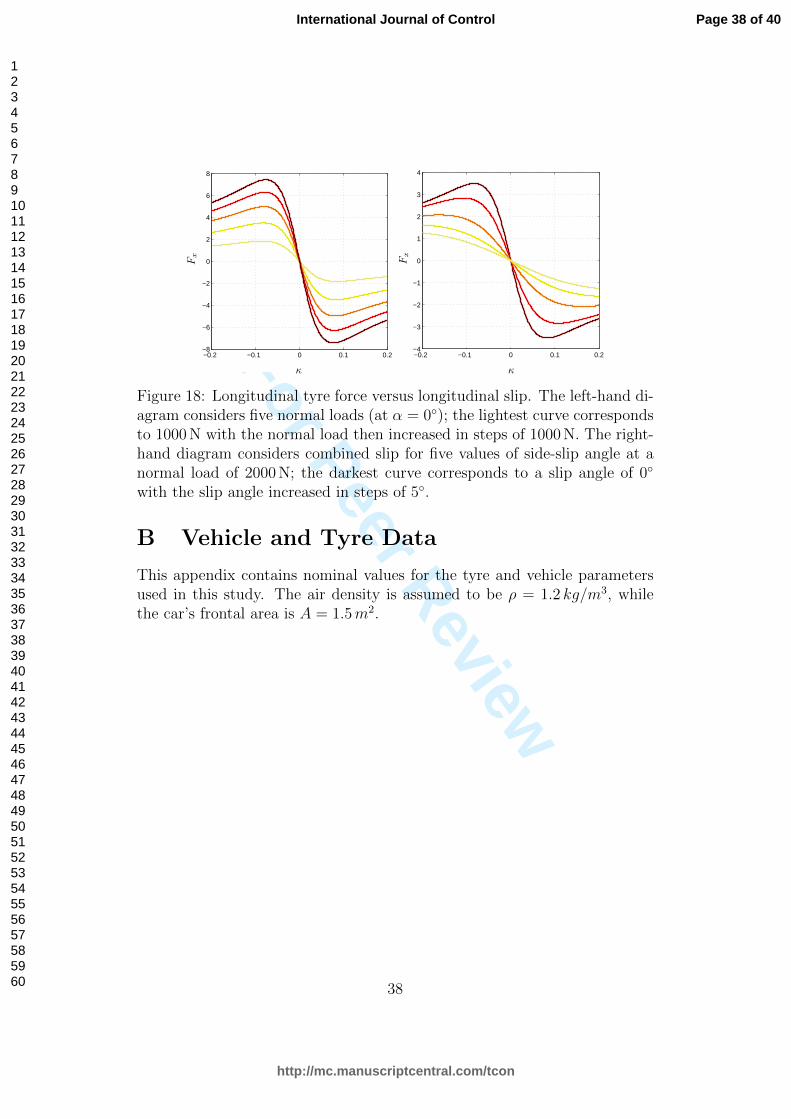
The left-hand part of Figure 18 shows the load dependence of the longi-tudinal tyre force under pure longitudinal slip conditions; larger longitudinalforces are available when the normal load is increased. The main reasonfor introducing aerodynamic down-force generating systems on Formula Onecars is to exploit this effect. The right-hand part of Figure 18 shows how thelongitudinal force is compromised when the tyre is side slipping. As the side-slip angle increases, the longitudinal peak force reduces and moves towardshigher slip values.

The normal-load-dependent inverted witch’s hat in Figure 19 gives a three-dimensional representation of the combined slip characteristics of the tyremodel at a fixed normal load of 2000 N. The tyre’s pure slip characteristicsare obtained by taking vertical cuts through the lines α = 0 and κ = 0.

37

Page 37 of 40



123456789101112131415161718192021222324252627282930313233343536373839404142434445464748495051525354555657585960

For Peer Review−0.2 −0.1 0 0.1 0.2−8

−6

−4

−2

0

2

4

6

8

κ

Fx

−0.2 −0.1 0 0.1 0.2−4

−3

−2

−1

0

1

2

3

4

κ

Fx

Figure 18: Longitudinal tyre force versus longitudinal slip. The left-hand di-agram considers five normal loads (at α = 0◦); the lightest curve correspondsto 1000 N with the normal load then increased in steps of 1000 N. The right-hand diagram considers combined slip for five values of side-slip angle at anormal load of 2000 N; the darkest curve corresponds to a slip angle of 0◦

with the slip angle increased in steps of 5◦.

B Vehicle and Tyre Data

This appendix contains nominal values for the tyre and vehicle parametersused in this study. The air density is assumed to be ρ = 1.2 kg/m3, whilethe car’s frontal area is A = 1.5m2.

38

Page 38 of 40



123456789101112131415161718192021222324252627282930313233343536373839404142434445464748495051525354555657585960

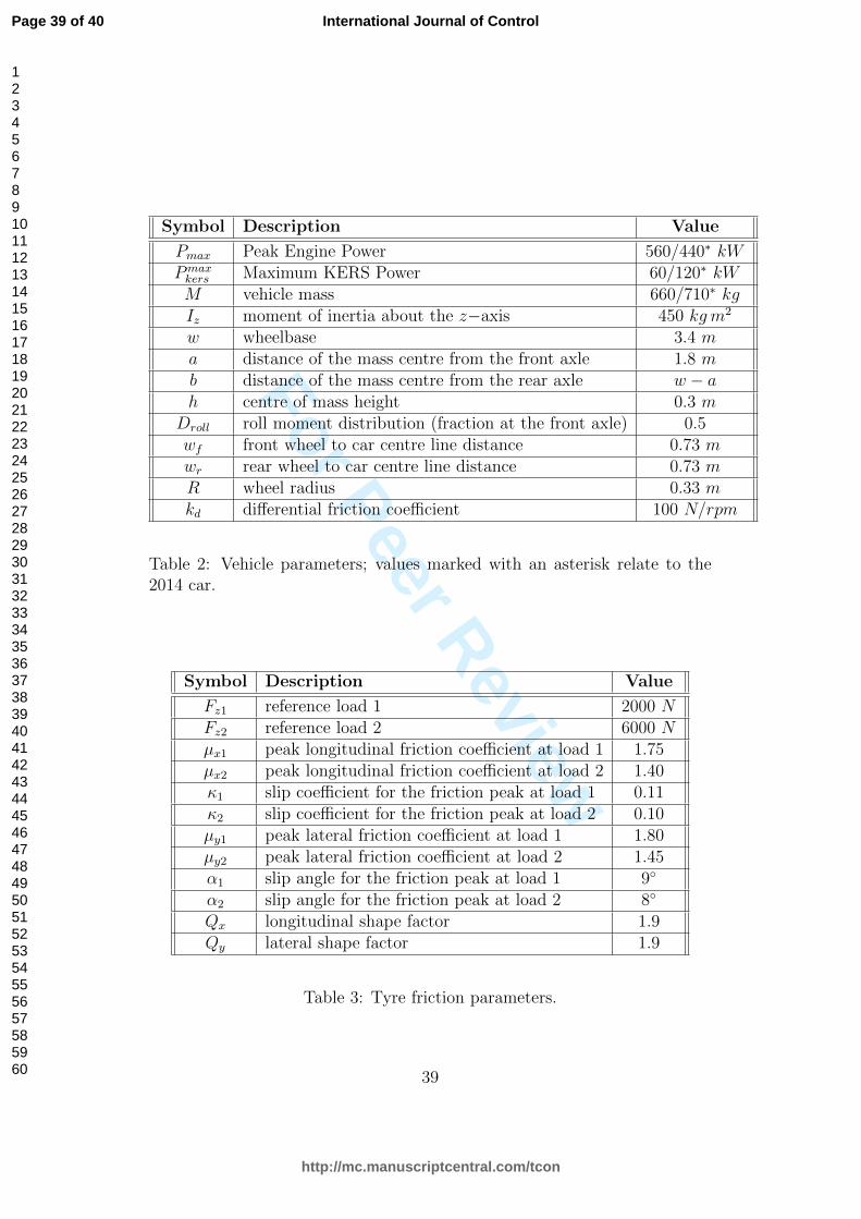
For Peer ReviewSymbol Description Value

Pmax Peak Engine Power 560/440∗ kWPmaxkers Maximum KERS Power 60/120∗ kWM vehicle mass 660/710∗ kgIz moment of inertia about the z−axis 450 kg m2

w wheelbase 3.4 ma distance of the mass centre from the front axle 1.8 mb distance of the mass centre from the rear axle w − ah centre of mass height 0.3 m

Droll roll moment distribution (fraction at the front axle) 0.5wf front wheel to car centre line distance 0.73 mwr rear wheel to car centre line distance 0.73 mR wheel radius 0.33 mkd differential friction coefficient 100 N/rpm

Table 2: Vehicle parameters; values marked with an asterisk relate to the2014 car.

Symbol Description Value

Fz1 reference load 1 2000 NFz2 reference load 2 6000 Nµx1 peak longitudinal friction coefficient at load 1 1.75µx2 peak longitudinal friction coefficient at load 2 1.40κ1 slip coefficient for the friction peak at load 1 0.11κ2 slip coefficient for the friction peak at load 2 0.10µy1 peak lateral friction coefficient at load 1 1.80µy2 peak lateral friction coefficient at load 2 1.45α1 slip angle for the friction peak at load 1 9◦

α2 slip angle for the friction peak at load 2 8◦

Qx longitudinal shape factor 1.9Qy lateral shape factor 1.9

Table 3: Tyre friction parameters.

39

Page 39 of 40



123456789101112131415161718192021222324252627282930313233343536373839404142434445464748495051525354555657585960

For Peer Review

κα

|F| 1

1.8

2.5

2.5

2.5

2.5

2.5

2.9

2.9

2.9

2.9

2.9

2.9

2.9

2.9

3.3

3.3

3.3

3.3

3.3

3.3

3.3

3.5

3.5

3.5

3.5

3.5

3.5

3.57

3.57

−0.2 −0.1 0 0.1 0.2−15

−10

−5

0

5

10

15

κ

α

Figure 19: Modulus of the tyre force as function of the longitudinal slip κand the slip angle α (in degrees) for a normal load of 2000 N. The right-handdiagram shows contours of equal tyre-force.

40

Page 40 of 40



123456789101112131415161718192021222324252627282930313233343536373839404142434445464748495051525354555657585960

Documents

For Peer Review Keywords - Home - Anil V. Rao's Website |vdol.mae.ufl.edu/.../F-1-Optimal-Control-Energy-Recovery.pdfFor Peer Review Optimal control of Formula One car energy recovery