(DVL+)

Automotive engineering TOOLBOX

for MATLAB/SIMULINK

Module: DVL-driver

(Version 10.2007)

Dr.-Ing. Aleksandar D. Rodić January 2012

All rights to the DVL-driver software toolbox belong to the IMP Robotics Lab. If you have some questions please refer to the following adress: Dr.-Ing. Aleksandar D. Rodić Head of Laboratory Mihajlo Pupin Institute Robotics Laboratory 11060 Belgrade SERBIA Tel.: +381 11 / 2776-174 Mobile: +381 63 / 331-927 E-mail: aleksandar.rodic@pupin.rs

1. PREFICE

From the point of view of mechanics, a vehicle represents a complex, distinctly nonlinear,

dynamic system with a relatively large number of degrees of freedom (DOFs), belonging to the class of large-scale dynamic systems. These DOFs (independent motion directions), especially those that essentially influence the system's stability and quality of its dynamic behavior, have to be controlled. The vehicle stability, quality of its dynamic behavior and maneuvering capabilities depend to a great extent on the structure of the system and performances of its power-actuating subsystems. Selection of a best control strategy and its realization, within the limits of technical capacities of the system, represents a delicate problem whose solving requires knowledge of dynamic behavior of the vehicle under different conditions of motion. To that end, mathematical model of the driver-vehicle system in the interaction with a dynamic environment represents a starting point in the stage of system design and its automatic control. That was the strong motivation for developing of the DVL+ automotive engineering toolbox. Its realization in the MathWorks’ Matlab/Simulink background gives it necessary simplicity for implementation in the design process, system analysis as well as in education.

2. WHAT IS DVL+?

The DVL+ represents user-oriented, Driver-Vehicle in the Loop (Fig. 1) modelling software operating in the MathWorks MATLAB/SIMULINK programming background. Algorithmic fundament of this software package is extended in particular by implementation (plus ‘+’) of the complementary knowledge based identification structures.

Figure 1: The structure of the hybrid, man-machine, i.e. driver-vehicle dynamic system

DVL+ automotive engineering toolbox has few functional software modules:

1) DVL – tyres 2) DVL - suspension 3) DVL – power drivetrain 4) DVL – vehicle dynamics 5) DVL - driver 6) DVL – full system

DVL – tyres software module represents non-linear, empirical model of tyre pneumatics based on Sakai or Pacejka researches. DVL – suspension software module is a linear or a non-linear model of vehicle suspension system. It includes tyre suspension as well as 4-wheel suspension system. DVL – power drivetrain software module represents the non-linear model of power drivetrain (traction) system of road vehicle including the particular models of: (i) IC engine (gasoline motor), (ii) automatic transmission system, (iii) vehicle drivetrain as well as (iv) planar vehicle dynamics. DVL – vehicle dynamics software module represents non-linear model of an entire road vehicle dynamics including vehicle body 3D- or 2D- dynamics, suspension dynamics as well as tyre dynamics. In that sense, this software module represents a software simulator of automotive system. DVL - driver software module represents empirical, non-linear model of psychological as well as physiological behaviour of driver as the human operator of a road vehicle. This module, apart to the driver model, also includes: (i) CAD-model of path geometry, (ii) model of driver-vehicle (man-machine) interface, (iii) model of power drivetrain system of a road vehicle as well as (iv) model of planar (longitudinal, lateral, yaw dynamics) vehicle dynamics. DVL – full system software module represents integrated modelling software including all previously mentioned software modules. In that sense, this module represents a software simulator of the entire (driver-vehicle in the loop) automotive system.

3. DVL – driver: USER GUIDE DVL-driver represents the most delicate and the most complex software module of the DVL+ automotive engineering toolbox. It represents a mathematical description of the driver behaviour in a realistic way. The present version of the driver modelling software is based on the research results disposable in the open scientific literature, author’s research experience in this field as well as on the own driving experience. Modelling software was designed to be simple for use and flexible for extension due to the research/developing requests. DVL-driver software, in present version, is suitable for simulation experiments as well as for possible real-time implementation. With experimental verification it will be a powerful tool for the synthesis of the advance, automotive control systems.

3.1 MATLAB VERSION ISSUES

DVL – driver was designed for the MathWorks MATLAB/SIMULINK, Version 6.5 Release 13, IBM PC compatible and Microsoft Windows XP. Also, it works with the younger versions of Matlab (e.g. Matlab 7.0, Release 14). DVL-driver uses standard Matlab functions as well as Simulink libraries. For a proper operation it needs only basic Matlab toolbox and Simulink. Remark: To use this modelling software, the basic knowledge of the Matlab/Simulink is necessary. In that sense, it will be considered that the customers are familiar with the Matlab/Simulink.

3.2 NECESSARY FACCILITY For installation and work DVL-driver needs PC Pentium IV at 2.4 [GHz], 512 Mb RAM with Windows XP as the operative system. Remark: It is recommended for a more comfortable work with DVL-driver, a PC Pentium IV with a faster microprocessor, e.g. at 3.0 or 3.2 [GHz], to be used. Due to the model complexity and numerical calculation the faster PC configurations are desirable but not obliged.

3.3 HOW TO INSTALL? Take the installation CD and copy the folder entitled “DVLdriver” to the hard disc of your computer. In such a way, you define the corresponding path where your modelling software will be situated (as for example C:|projects\DVLdriver\).

3.4 HOW TO START? Start the Matlab and set the Matlabpath as C:\projects\DVLdriver\ including all belonging subfolders: 22dof, images, Powtrain, Tyremod, driver, paths, suspsys and vehibody. Check if you have already installed Simulink!? Before start of the Simulink, choose the root folder C:|projects\DVLdriver\. The main Simulink model DVLDriverModel.mdl exists at this level. Then, start the Simulink. Apply OPEN command of the Simulink to open the modelling task entitled: DVLDriverModel (use the browser for this purpose). After running the program, the following screen, as it is presented in Fig. 2, should to appear. Then, simply click on the field SIMULATION, and after that click the START (see Fig. 2). The driver modelling programme will run on.

Figure 2: The main screen of the driver modelling software DVL-driver 3.5 GRAPHICAL INTERFACE DVL-driver use Matlab and Simulink graphical interface to plot (monitoring) the system variables. DVL-driver software module calculates in every cycle of simulation more than 100 variables. Author of the software choose for demonstration only particular of them that are characteristic and interesting for the analysis. Of course, all of the variables (input, output, intermediate) can be plotted depending on user choice. During the program operation the following plots can be observed in this case: (i) the current position of a road vehicle along the desired path and (ii) the plots (graphs) of the particular important variables. The current position of the vehicle along the desired path is presented by the plots shown in the Figs. 3 and 4.

Global view of the test path as well as the position of the vehicle is presented in Fig. 3. Black line represents the desired (imposed) path of the vehicle. Red square is the current position of the car. Blue squares represent the STAT and the END points of the desired lane. Green signs “*” and “+” in Fig. 3 represent the current position of the Preview Point on the road as well as the position of the point denoting the Safe Stop Point of the vehicle. Both points have an essential importance for calculation of the driver model.

Figure 4 represents the “zoom” of the sector [+50,-50] m in the neighbourhood of the current mass centre position of the car (Fig. 3). The black line denotes the desired path while the red one denotes the actual trajectory of the vehicle, too. Measuring the shortest distance between these two paths (black one and red one) user can estimate the quality/accuracy of the driving skill. Green asterisk “*” denotes, as well as in the Fig. 3, the current position of the Preview Point of the car. Yellow circles ‘o’ on the front side of the car indicate the front (right

and left) position lights of the vehicle. In such a way, one can make difference at the plots between the front and the rear part of a car in all driving situations.

Figure 3: Plot of the global view of the desired path in one characteristic time instant of simulation

Figure 4: Zoom of the particular sector (shown in Fig. 3) whose centre is in the

current vehicle position (mass centre of road vehicle) Figures 3 and 4 includes certain alphanumerical symbols in the left lower edge of graphs

denoting the actual forward speed of the car [km/h], passed time of driving [sec] and passed

effective distance from the start in [m]. Forward speed of the vehicle can be observed by the plot entitled “[1] Forward speed”, too, as it will be explained in the text to follow.

Plots that are presented in Figures 3 and 4 are periodically exchanged each other in order to present the actual situation on the road, i.e. exact location of road vehicle along the desired trajectory. Particular variables of interest can be viewed by the time-plots as it is shown in Fig. 5 by black plots. In this case, the modeling software shows the following plots although all the other can be also viewed: [1] Forward speed [km/h] [2] Longitudinal & lateral acceleration [m/s^2] [3] Yaw angle & yaw rate [deg] or [deg/s] [4] Tyre slip ratio [5] Tyre shaft torque [Nm] [6] Gear box level [7] RPM engine [1/min] [8] Engine torque [Nm] [9] Side slip angle [deg] [10] Steering wheel angle [deg] [11] Ground steering angle [deg] [12] Braking force [N] [13] Throttle position [rad] [14] Side error of path tracking [m] [15] Longitudinal tyre forces Fxi, i=1,4 [16] Lateral tyre forces Fyi, i=1,4 To view any of the mentioned graphs just you need to do is to simply click at the bottom window of the screen entitled “matlab” (see Fig. 5). Then, let choose a variable or plot from the offered list by click on the corresponding title with a left mouse key. In order to get a better insight in to the variables interesting for us to be viewed, look to the Fig. 6 that shows the relative position of a car along the imposed path. To judge the quality of driving car let observe the following variables as the results of numerical simulation: side (lateral) error of path tracking (see Fig. 6), forward speed of road vehicle (see Fig. 6), longitudinal & lateral accelerations (x- and y-directions, see Fig. 6), side slip angle of road vehicle (see Fig. 6), yaw angle (see Fig. 6) and yaw rate, etc. In that sense, in the following subsection there will be speak a little bit about criteria that was imposed to be satisfied designing a driver model.

Also, here will be mentioned the input as well as the output variables of the simulated model. As input signals to the driver model are taken: (i) variables that describe the changes of path geometry (certain distances and angles), (ii) current relative position of the road vehicle with respect to the desired path as well as (iii) state variables of vehicle dynamics (forward speed, acceleration, side slip angle, yaw angle, yaw rate, etc). Output variables of driver model are: (i) steering wheel angle, (ii) throttle position (as a consequence of pressing the acceleration pedal), (iii) braking force at the braking pedal. Beside the input and output variables some other interesting variables are enabled to be displayed via plots (Fig. 5) such as: tyres’ slip ratios, tyre forces, engine torque, RPM of engine, etc. Of course, the focus of attention is primary directed before all to the input and output variables of driver model because it is central point of the DVL – driver software module.

Figure 5: Graphic interface of the Simulink used to analyze of the simulation variables

Figure 6: Relative position of a road vehicle along the desired path - some characteristic variables interesting to be displayed by graphs during motion

3.5 MODUS OF OPERATION & MODEL PARAMETERS Driver model was designed as an empirical MIMO (multi input – multi output), non-linear function whose parameters were determined according to the real driving experience (experimental measurements are necessary) as well as according to the numerous simulation experiments. In that sense the following driving criteria were imposed to be satisfied: 1) Criterion of minimal side (lateral) error of road vehicle as small as possible along the

chosen desired path geometry, 2) Criterion of a fine speed adaptation to changes of the path geometry, 3) Criterion of a limited lateral acceleration, 4) Criterion of limited speed of motion, 5) Criterion of a fine driving comfort avoiding large yaw rate, large side slip angle as

well as prevention of jerky motion. Remark: In this version of DVL-driver, algorithm for avoiding fixed (e.g. rock on the road) and mobile obstacles (low speed vehicles) existing on the road was not jet synthesized. This problem can be solved successfully in the next versions of the DVL-driver modelling software extending the existing algorithms. According to the assumed driving criteria the four driving modus can be defined and tested in simulation experiments. These are:

1) Defensive driving 2) Offensive driving 3) Driving with constant speed 4) Non-skill driver

Defensive driving concerns such set of driver model parameters that enables careful driving with small side (lateral) errors (fine tracking of desired path), moderate forward speed of motion, lateral acceleration less then for example 0.25*g (g is a gravity acceleration) and without hazard motion (large yaw rate and slipping). Offensive driving represents such set of model parameters that ensures a “sporting way” of driving tests with “faster path” but generally with larger side errors (as a consequence) then in the case of a defensive modus. Such kind of driving assumes less trajectory tracking accuracy but faster path and possible appearance a hazard motion in certain situations. The limits for lateral acceleration, yaw rate as well as for the side slip angle of road vehicle are enlarged in comparison to the modus 1). Driving with constant speed is the third modus that satisfies only one criterion – running with conditionally constant (with small variation) forward speed of a road vehicle. This modus is suitable for certain simulation tests where the analysis of a vehicle dynamics in cornering manoeuvres or driving slalom is demanded. Non-skill driver modus takes model parameters that enable simulation of the behaviour of a non-skill driver (an aged driver or a driver beginner). This modus takes into account larger amounts of time delays in psychological and physiological reactions of human driver, non-adequate control gains of manual commands, bad adaptation to changes of road geometry, etc.

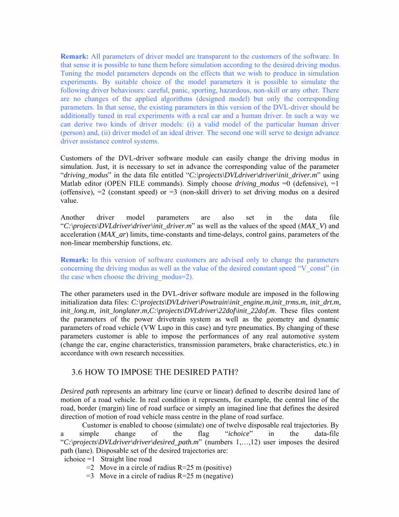
Remark: All parameters of driver model are transparent to the customers of the software. In that sense it is possible to tune them before simulation according to the desired driving modus. Tuning the model parameters depends on the effects that we wish to produce in simulation experiments. By suitable choice of the model parameters it is possible to simulate the following driver behaviours: careful, panic, sporting, hazardous, non-skill or any other. There are no changes of the applied algorithms (designed model) but only the corresponding parameters. In that sense, the existing parameters in this version of the DVL-driver should be additionally tuned in real experiments with a real car and a human driver. In such a way we can derive two kinds of driver models: (i) a valid model of the particular human driver (person) and, (ii) driver model of an ideal driver. The second one will serve to design advance driver assistance control systems. Customers of the DVL-driver software module can easily change the driving modus in simulation. Just, it is necessary to set in advance the corresponding value of the parameter “driving_modus” in the data file entitled “C:\projects\DVLdriver\driver\init_driver.m” using Matlab editor (OPEN FILE commands). Simply choose driving_modus =0 (defensive), =1 (offensive), =2 (constant speed) or =3 (non-skill driver) to set driving modus on a desired value. Another driver model parameters are also set in the data file “C:\projects\DVLdriver\driver\init_driver.m” as well as the values of the speed (MAX_V) and acceleration (MAX_ar) limits, time-constants and time-delays, control gains, parameters of the non-linear membership functions, etc. Remark: In this version of software customers are advised only to change the parameters concerning the driving modus as well as the value of the desired constant speed “V_const” (in the case when choose the driving_modus=2). The other parameters used in the DVL-driver software module are imposed in the following initialization data files: C:\projects\DVLdriver\Powtrain\init_engine.m,init_trms.m, init_drt.m, init_long.m, init_longlater.m,C:\projects\DVLdriver\22dof\init_22dof.m. These files content the parameters of the power drivetrain system as well as the geometry and dynamic parameters of road vehicle (VW Lupo in this case) and tyre pneumatics. By changing of these parameters customer is able to impose the performances of any real automotive system (change the car, engine characteristics, transmission parameters, brake characteristics, etc.) in accordance with own research necessities.

3.6 HOW TO IMPOSE THE DESIRED PATH?

Desired path represents an arbitrary line (curve or linear) defined to describe desired lane of motion of a road vehicle. In real condition it represents, for example, the central line of the road, border (margin) line of road surface or simply an imagined line that defines the desired direction of motion of road vehicle mass centre in the plane of road surface.

Customer is enabled to choose (simulate) one of twelve disposable real trajectories. By a simple change of the flag “ichoice” in the data-file “C:\projects\DVLdriver\driver\desired_path.m” (numbers 1,…,12) user imposes the desired path (lane). Disposable set of the desired trajectories are: ichoice =1 Straight line road =2 Move in a circle of radius R=25 m (positive) =3 Move in a circle of radius R=25 m (negative)

=4 Move along ellipse =5 Driving piranha slalom =6 Change lane manoeuvre (example of avoiding obstacle) =7 Double change curves (curve-linear path) =8 Street corner of 90 degrees =9 Arbitrary defined curvilinear closed path =10 Driving along the "Verkehr Testuebung Platz" in Braunschweig =11 Driving around the "Nuerberger Ring" racing path (Mini ~1.7 km) =12 Driving around the "Nuerberger Ring" racing path (Full ~5.1 km) … Other ones or user own path ... Images of the previously described desired paths are given in the Figs. 7 and 8.

Figure 7: CAD models of path geometry of desired trajectories ichoice=1,…,6

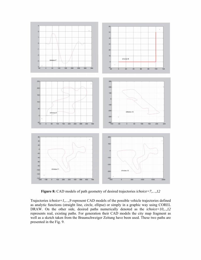
Figure 8: CAD models of path geometry of desired trajectories ichoice=7,…,12 Trajectories ichoice=1,…,9 represent CAD models of the possible vehicle trajectories defined as analytic functions (straight line, circle, ellipse) or simply in a graphic way using COREL DRAW. On the other side, desired paths numerically denoted as the ichoice=10,..,12 represents real, existing paths. For generation their CAD models the city map fragment as well as a sketch taken from the Braunschweiger Zeitung have been used. These two paths are presented in the Fig. 9.

Figure 9: Images of the real paths “Nuerberger Ring” and “Braunschweiger Verkehrsuebungplatz” taken for designing CAD models of the desired paths numerated as ichoice=10, 11 and 12

Customers are also enabled to design (create) their own desired paths to be simulated. It is possible to do analytically using Matlab functions or graphically using some of the graphic programs such as COREL DRAW. All that is necessary to do is to generate the matrix “path” in the Matlab work-space. The order of the path-matrix depends on the path length. Generaly, matrix order has to be path(1:N,1:4) where N is a number of data samples of the desired trajectory. The first two columns of the matrix path(1:N,1:2) are X and Y coordinates of the desired path with reference to the initial coordinate system (see Fig. 6). Note that the X-axis in the zero time instant (t=0) is always directed along the longitudinal x-axis of a road vehicle. The third column of the matrix path(1:N,3) represents vector of the yaw angles along the desired path expressed in radians (see Fig. 6). It is possible to design as well open as closed trajectories in a way that was presented in Figs. 7, 8, and 9. Yaw angle values should be in the interval [ ]ππε 2,2 +−∈ . The last column in the matrix path(1:N,4) represents vector of the successive effective distance from the path begins. It is advised that the distance increments should be chosen to be ~0.10 [m]. It is important to stress out that the yaw angle hodograph along the designed trajectory must not have discontinuity (to be smooth) to enable the modelling programme to work without troubles (accurately). Matrix path(1:N,1:4), after calculation of all rows and columns, should to be saved as a new desired path using the Matlab command save FileName path; Also, in the data file “desired_path.m” the command load FileName; should to be added in order to enable simulation of the new defined trajectory.

3.7 SIMULATION EXPERIMENTS DVL-driver software module enables various extensive simulation experiments with different desired trajectories. Customer can define arbitrary car parameters as well as to change the driving modus: offensive, defensive, constant speed or non-skill driver. In that sense, it is possible to make simulation driving tests in different conditions and with different set of

parameters. Main indicator of the trajectory tracking accuracy is side (lateral) error of path tracking. Also, important variables are: forward speed, yaw rate, side slip angle, longitudinal and lateral acceleration along the desired path. Driver model, as a MIMO function, at its output generates the following commands (signals): steering wheel angle, throttle position (acceleration pedal) and braking force at the braking pedal. These commands are forwarded to the driver-vehicle interface: steering system, traction system (engine and drivetrain) and braking cylinders. As it was mentioned in the previous consideration, a monitoring of all variables is possible using Matlab/Simulink graphic interface. At the end of a simulation task (when the road vehicle reaches the end pint of the desired path) a textual messages appear on the screen as it is presented in Fig. 9.

Figure 10: Final messages of the simulation task indicating the accuracy of the driving test The messages include information about: (i) Maximal side (lateral) error of trajectory tracking in [m]; (ii) The exact position where the maximal lateral error has appeared in the initial coordinate system in [m]; (iii) Average side error along the desired path in [m]; (iv) Average forward speed of road vehicle in [km/h]; (v) Average slip angle of road vehicle during motion in [rad]. All of these variables (its absolute values) are also displayed during simulation. End of simulation, i.e. reaching the end point of the desired path is accompanied with the set of successive beep signals in order to alert the user to stop the task. Beep can be switched off by changing the flag beep_kraj=1 to be beep_kraj=0 in the data file “init_driver.m”.

3.8 MODELING OF SYSTEM PERTURBATION DVL-driver enables simulation of external disturbances that act on the system behaviour during motion. As external perturbations of the system the following ones are considered: (i) slope of the road, (ii) slippery road and (iii) side wind gust. Slope of the road represents a longitudinal inclination of a road surface with respect to the horizontal plane. Slope influences upon the forward speed of motion of road vehicle. In that sense, vehicle driver have to adopt the commands of acceleration as well as braking to the real situation on the road. Slippery road represents one of the most significant perturbations acting on the automotive system. Due to the different conditions of a road surface (wet, ice, oil) the Coulomb’s friction coefficient of tyre-road interaction is changed. It influences the vehicle dynamics especially during cornering or fast moving and braking. In this case, driver have to adopt forward speed of road vehicle as well as steering wheel angle to the actual surface conditions. Side wind gust can be very dangerous perturbation in the case of a strong blowing or changing its direction. Real car are designed to have the air resistance as small as possible. In spite of this fact, blowing impact forces cannot be prevented. Simulink blocks for modelling (simulation) of system perturbations are presented in Figs. 11 and 12.

Figure 11: Simulink blocks – model of power drivetrain system, model of vehicle dynamics and models of external disturbances

By double clicking at the left mouse key, with a previous positioning on the Simulink block “Model of vehicle dynamics” (see the mask in Fig. 2), one enters in to the lower level (Fig. 11). In the lower left edge of the screen (marked by a red circle) three Simulink blocks exist. These blocks represent models of system perturbations (Fig. 12).

Figure 12: Simulink blocks – models of external disturbances By selection of the first block entitled “Slope of road surface” and double clicking on it, the following interactive Simulink dialog is opened (see Fig. 13). Using a slider gain customer choose a slope angle of a road surface as a percentage of maximal angle value (it is 90 [deg]). In the Fig. 13, as an example, the 10% of 90 [deg] was imposed. That represents absolutely 9 [deg]. In a similar way, using slider gains again, the tyre friction coefficients can be changed as it is shown in Fig. 14. Double click by mouse on the block entitled “Tyre-road interaction” (Fig. 12). The Simulink block shown in the Fig. 14 is opened. Using manual switch choose the desired combination of friction changes. Upper position of the manual switch enables different (split) friction distribution at four tyres. Lower position ensures the same friction at the corresponding pairs of right as well as left side tyres. The rear and front tyres of one side has the same friction conditions. Using slider gains choose the desired friction coefficient in the interval [ ]1,0∈μ . For 1=μ the road surface is absolutely dry and clean while for 0=μ it is absolutely slip. The real values should be between 0.30 and 1.00. For example in the Fig. 14 the friction of the first tyre (front right wheel) is chosen to be 73.0=μ that corresponds to the wet road. In the case of icy road or oily surface the value of 30.0=μ should to be introduced.

Figure 13: Model of the slope of a road surface

Figure 14: Model of the slippery road (split friction of tyres)

By a double click on the Simulink block entitled “Model of side wind gust” shown in Fig. 12, corresponding model is opened as it was presented in Fig. 15. Concerning the model of wind gust, two variables as inputs are necessary to be defined: (i) wind speed in [km/h] and, (ii) wind direction in [rad]. Using slider gain, customer is able to choose the speed of wind blowing (e.g. 44 km/h, see Fig. 15). The corresponding wind impact forces depend on the speed of wind blowing. Direction of wind blowing can be imposed defining the value of corresponding angle. As an example in the Fig. 15, angle of 6/2π [rad] was assumed. Zero value corresponds to the blowing direction that is collinear with the 0X -axis of the absolute coordinate system (Fig. 6). The angle changes in the direction opposite to clock wise.

Figure 15: Model of the side wind gust

Remark: Simulink model DRVDriver.mdl is initially set to the case of vehicle motion on a horizontal plane. Tyres’ friction is imposed to correspond to the case of motion over the clean and dry asphalt.

Remark: In the case of certain confusion in understanding of this user guide or in the course of work with the DVL-driver modeling software please contact the author using the e-mail given at the front page.