NASA Contractor Report 178301

TECHNICAL BACKGROUND FOR A DEMONSTRATI ON

MAGNETIC LEVITATION SYSTEM

[NASA-CR-178301) T E C H N I C A L B A C K G R O U N D P3B A N8 7- 2 53 32 DE#ON STRATI3N HASNETIC L E V IT ATION SYS 3: EM ( o l d Doatinion Univ . ) 38 p Avail: NTIS 3C A03/HF A01 CSCL 14a Unclas

S33/09 0079474

C o l i n P . B r i t c h e r

OLD DOMINI ON UN I VE RS I TY N o r f o l k , V i r g i n i a

Grant NAG1-716 May 1987

National Aeronautics and Space Administration

Langley Research Center Hampton,Virginia 23665

https://ntrs.nasa.gov/search.jsp?R=19870015899 2018-08-25T11:12:39+00:00Z

CONTENTS

.

1. Introduction

1.1 Statement of problem 1.2 Background - wind tunnel MSBSs 1.3 Comparative technical difficulty of MSBS and ML

2. General design approach

2.1 Choice of model core 2.2 Magnetic configuration 2.3 Other hardware

3. Magnetic theory

3.1 Force and moment production 3.2 Magnetic couplings

4. Preliminary magnetic design and optimization

4.1 Simple, uncontrolled levitation

4.1.1 Choice of superconductor specifications 4.1.2 Two-electromagnet levitation analysis 4.1.3 Copper electromagnet feasibility

4.2 Controlled, single point levitation

4.2.1 812+688 electromagnet configuration 4.2.2 816+088 electromagnet configuration

5. Further magnetic design

5.1 Roll control 5.2 Yaw angle requirement

6. Operational considerations

6.1 Stray magnetic fields 6.2 Reliability

7. Discussion

References

Appendix 1 Computational capability - FORCE etc.

i

1 INTRODUCTION

1.1 Statement of problem

It is required to somehow suspend or levitate an aerodynamic model in such a way that a large clear air volume can be maintained around the model. It has been decided that this could be achieved most satisfactorily if all levitation/suspension hardware were positioned on or behind a single plane surface, at some distance from the center of the model. This distance would be of the order of 3 to 4 feet. Further, there appears to be some advantage in choosing the floor to be the plane surface, forming a Magnetic Levitation (ML) system (Fig.l.1). This report represents a preliminary assessment of the technical feasibility of such a system.

the levitated model. Rather small aerodynamic or other loads are anticipated. The model's spatial position and orientation are to be maintained to high accuracy, with very small allowable undemanded motion around any particular location. The position and attitude must, however, be variable, under operator control, preferably over a wide range. The rate of movement from one position/attitude to another may be relatively slow.

The model's own weight will be the principal force acting on

1.2 Background - wind tunnel MSBSs models (MSBS) have been under development for nearly 30 years. Around 15 systems have been constructed by ten different institutions, worldwide (Ref.1). Only four systems are presently known to be operational :

Magnetic Suspension and Balance Systems for wind tunnel

13 inch NASA Langley Research Center ( formerly AEDC) 6 inch MIT/NASA Langley Research Center 7 inch University of Southampton 3 inch Oxford University

General features common to all known systems include small physical scale, the 13" LaRC system being the largest yet constructed, and relatively low magnetic force capability, typically less than 5 times the weight of the model's magnetic core. With the exception of the second University of Virginia system, all have utilized conventional copper electromagnets, with or without forced cooling. Two systems (Southampton and 13" LaRC) are equipped with digital control systems, otherwise simple analogue controllers have been used. A wide variety of techniques for sensing the position and attitude of the suspended model have been employed, including many types of optical system, electromagnetic sensors and X-rays. Still more techniques have been proposed, though no system currently in operation can be regarded as entirely satisfactory. Model magnetic cores have been soft iron or permanent magnet, though a superconducting solenoid has been demonstrated.

1

Design studies of Large MSBSs (LMSBS) have been performed recently, (Refs. 2,3,4) with the important conclusion that systems for wind tunnels up to 8 foot test section size are feasible with essentially existing technology, though potentially costly to construct.

1.3 Comparative technical difficulty of MSBS and ML

A comparison of this type is appropriate and illuminating.

Physical scale

Although existing MSBSs are all relatively small, the design studies presently available give a high degree of confidence that large scale facilities (up to 8-foot test section size) could be successfully constructed. The single major technical change required for the larger scale systems, compared to existing MSBSs, would be the replacement of the usual copper electromagnets with superconducting electromagnets. This is for two important reasons:

1) Creation of the relatively intense magnetic fields

2) Power economy. The steady state power consumption of

required to oppose the high aerodynamic loads on the model.

copper electromagnets increases rather rapidly as system size increases and can become outrageous. This problem is perhaps the more relevant for ML.

Force and moment capability

MSBSs have to be capable of magnetically opposing uncontrolled and unknown aerodynamic loads on the model. These loads can be large with respect to the model's mass and will be so in LMSBSs. The absence of these loads in the ML application has two important effects :

1) Reduction of required intensity of magnetic fields and field gradients. This apparent advantage is, however, offset to some degree by the restrictions on location of the levitation electromagnets.

requirements. MSBSs have to be able to counter rapidly changing aerodynamic loads and usually are capable, as a result, of driving the model through operator demanded, oscillatory motions of significant amplitude and frequency. Quasi-steady, undisturbed levitation is possible with substantially reduced dynamic capability, notably in the area of electromagnet power supplies.

2) Considerably reduced dynamic force and moment

Position/attitude precision

The required precision for MSBS and ML appear to be somewhat similar, specifically of the order of thousandths of an inch in

2

position and hundredths of a degree in orientation. This has been achievable for many years with MSBSs, albeit under controlled conditions. Long-term drift has been the most difficult problem, almost entirely related to position sensing techniques. New approaches in this area promise to eliminate this difficulty.

A model in an MSBS can never be absolutely stationary, since the systems are open-loop unstable and rely on position and attitude error feedback for stabilization. The exact amplitude of motion of the model around a set-point is a strong function of the amplitude of the disturbances acting on the model (aerodynamic etc.), the quality of electromagnet power supplies, the resolution of position sensors and the sophistication and adjustment of the control system. With wind-off (low disturbances), extremely steady suspension has been observed at the University of Southampton (certainly +- O.OO1l l position). Fairly good results have been measured with the 13" LaRC MSBS (+- 0.00311 position) despite several recognized shortcomings in hardware (Fig. 1.2)

Position/attitude range

MSBSs have mostly been restricted to a rather small range of model positions and attitudes. The exact ranges have generally been set by position sensor capability, but there are fundamental restrictions caused by the gross variation in magnetic couplings between electromagnets and model that occur with large angular or translational motion. This difficulty has been addressed at some length in Ref.5 and limited but successful demonstrations have been made of extreme attitude capability (Fig.l.3). Extensive further work in this area is required and some is understood to be underway at Southampton. It is, however, confidently stated that there is no fundamental limit to model position or attitude capability, provided that :

3 )

The correct magnetic field and field gradient components can somehow be created in the appropriate strengths and combinations.

The extensive couplings between model degrees of freedom that occur due to the powerful and variable magnetic couplings can somehow be accomodated.

The position, attitude and trajectory of the model can be accurately monitored.

Control systems

MSBSs utilize multi-loop control systems of the general form shown in Fig.l.4. Control algorithms may be implemented digitally or by analogue circuitry. This general form is certainly applicable to ML. The compensation algorithms (series lead-lag) universally used to date are somewhat antique, but can be made to perform well with some care in adjusting gain and frequency parameters. It is felt that ML can be expected to operate successfully with this form of algorithm and, with a digital control system, new algorithms can easily be installed whenever they become available.

3

The lrprefilterr' and "translatorrr functions will not be trivial for ML. They exist so that the controller can operate in model degrees of freedom, strongly felt to be the best approach. If the model is to be capable of large attitude or position excursions, then the prefilter and translator become large matrix operators with variable coefficients. The general theme explored in Ref.5 was that these coefficients could be pre- calculated to adequate accuracy and adjusted in real-time by using look-up tables or programmed functions or a combination thereof in a control computer. This has never been demonstrated experimentally, though suspension at various discrete attitudes was acheived with pre-calculated de-coupling/coupling terms in the prefilter and translator.

Data acquisition

In the wind tunnel application, whole-body aerodynamic force and moment data may be acquired by monitoring the electromagnet currents and comparing to previous calibrations. Lack of efficient calibration techniques has been a long standing and unresolved difficulty. This kind of calibration and data acquisition is not required in the ML application.

Electromagnet power supplies

Power supplies have been a source of many problems in MSBS development (Power supply is actually something of a misnomer, the proper description being power amplifier, since controlled currents must be supplied to the load electromagnet by varying the amplifier output voltage). Current and voltage requirements can be rather high, many kVA even at small scale, and frequency response must extend to a few tens of cycles per second. The load current must be relatively smooth for high quality control of model position although the high inductances typical of large electromagnets is of assistance here. These are demanding specifications but can be met by power supplies intended for large D.C. servomotor drives. Units are known to be commercially available up to around 500 kVA rating (1000 Amps, 500 Volts). The most difficult requirement for MSBSs has been for bipolar operation. This arises partly since the weight of the model can be relatively small compared to other loads, thus the electromagnet currents required merely to suspend the model (wind-off) are low. Further, as the model is maneuvered over a range of attitudes, large changes, including sign reversals, of electromagnet currents are encountered. Since the model's weight is the dominant force in ML, monopolar current capability, at least in some electromagnets, may prove to be adequate, though the magnetic coupling changes with attitude and position variations require careful study in this regard.

Magnetic configuration

Advanced MSBS designs tend to develop as a tightly packed array of many electromagnets surrounding the wind tunnel test section. The geometry and configuration of these electromagnets

4

is crucially important for several reasons :

1) Creation of the required field and field gradient

2) Achievement of 1) with high efficiency 3) Achievement of 1) with predictable and manageable

components.

magnetic couplings over the required range of model positions and attitudes.

The same requirements apply to ML systems, though the designer's freedom to locate electromagnets around the model is seriously reduced.

Summary

With the sole exception of magnetic configuration, it is seen that ML is of comparable or lower technical difficulty than LMSBS. Synthesis of an appropriate magnetic configuration is essentially an intellectual problem, to be tackled and resolved in the early phases of design. The technical risk for an ML system, meeting the broad specifications and operational requirements presently considered, is therefore judged to be relatively low.

5

Permanent magnet model core

4 feet (Model center to electromagnet face)

lectromagnet array

W

Fig.l.1 Demonstration magnetic levitator - conceptual

0.003"

I

I 0.001"

Southampton MSBS Vertical displacement

NASA Langley 13" MSBS Axial displacement (top) Lateral displacement (bottom)

1 0.0 0.1 0.2 0.3 0.G

Seconds

0.0 0.4 0.8 1.2 1.6

Seconds

Fig.l.2 Demonstrated steadiness of model suspension

6

Fig.l.3 High angle-of-attack suspension with MSBS

Multiple electromagnets and power supplies

/ Allaca Force and moment demands

STABILIZATION

Usually series lead-lag

Operator Multiple PRE- FILTER demands position

attitude model degrees Position and sensors of freedom attitude

, . = and > Decouple to '

- information

Fig.l.4 Typical MSBS control loop

7

2 GENERAL DESIGN APPROACH

2.1 Choice of model core

Three options are available for the magnetic core of the levitated model :

1) Permanent magnet 2) Soft-iron 3) Persistent superconducting solenoid

All have been used to various degrees with MSBSs. Soft-iron cores have been utilized in two fundamentally different ways, one being operation in an attraction mode (eg. 13" LaRC), where the required magnetization of the iron is naturally achieved by the applied fields, as shown in Fig.2.l. Alternatively, the magnetization can be artificially introduced by quasi-uniform applied fields (eg. 611 MIT/LaRC), also illustrated in Fig.2.1. This is normally only successful if the subsequently applied fields and field gradients exhibit a certain degree of symmetry, otherwise the induced magnetization may be lost.

The requirement to levitate the model above a plane floor in this application suggests operation in a repulsion mode. Further, there appears little possibility of elegantly achieving the required uniformity of magnetizing and symmetry of other fields from the restricted available locations of electromagnets. Option 2) above is therefore dismissed.

For large scale applications, a persistent superconducting solenoid has some advantages. The high levels of effective magnetization that are attainable would result in significant economies in the sizing and powering of the levitation electromagnets. A solenoid of representative scale has already been successfully operated in a small MSBS (Ref.6). Technical difficulties in the use of superconducting solenoids in MSBSs include limited run-time (of the order of 1 hour), helium venting, calibration uncertainties and mechanical design to sustain high loads. The levitation application does not require high load capability, nor force and moment calibration and the residual difficulties of run-time and helium venting are regarded as relatively minor development problems. Unfortunately, the performance of superconducting solenoids is very sensitive to scale, improving rapidly, relative to alternative core materials, with increasing scale.

For the scale of device presently envisaged, the appropriate choice of core material is felt to be permanent magnet. Powerful, stable materials are available (Rare-Earth Cobalts) in large sizes (at least 2" dia. by 0.511 length, stackable) The control and dynamics of a superconducting solenoid are virtually identical to a permanent magnet model, thus a superconducting solenoid could be utilized later, providing a performance upgrade of some sort, if required.

Earth Cobalt materials are taken to be: At the present time, representative properties for Rare-

..

Magnetization (Saturation Induction) 1 Tesla Density 8 000 kg/m3 Coercive force (greater than) 800 kA/m Magnetic stability Very good Mechanical properties Hard, brittle

The only problems that are likely to be encountered are the mechanical brittleness and the the fact that the magnet cannot be "turned off", presenting certain cleanliness and housekeeping problems.

2.2 Maanetic confisuration

The general requirement has been concluded as being that of levitation of a model in %ormal1I orientation (that is, major axis horizontal) by an array of electromagnets buried beneath a plane floor (Fig.l.1). This configuration is expected to be statically unstable (that is with steady magnetic fields) in several degrees of freedom. Vertical translation and pitching rotation may be stable, provided other motions are suppresed. Roll rotation may be neutrally stable with axisymmetric models or positively stable with the model center of gravity set lower than the magnetic center. Now, some open-loop unstable degrees of freedom are always present in magnetic suspension systems of this general class. Further, any stable degrees of freedom tend to exhibit unsatisfactorily low damping. Feedback control of all degrees of freedom, providing artificial stiffness and damping, is the normal and correct approach, thus the extensive open-loop instabilities of this configuration are of no particular concern.

It is desired to control the model over a significant range of attitude, perhaps :

Pitch : +- 20 degrees Roll : +- 20 degrees Yaw (Azimuth) : 360 degrees

Since the levitated model is part of a control loop, some angular motion is naturally available. Experience with MSBSs indicates that the pitch and roll requirements shown above might be met with little difficulty. The azimuth requirement is significantly more challenging. Presuming that the model position and attitude can be accurately monitored over the required range, itself not a trivial task, the synthesis and verification of appropriate electromagnet configurations and development of decoupled control algorithms still remain as serious difficulties. These points are discussed more fully in Section 5.

2.3 Other hardware

Sufficient experience already exists in the use of digital control systems with MSBSs to conclude that a digital controller is the correct choice for ML. The control task can be considered as being divided into three main sections (after Ref.7):

9

1) Stabilization 2) Operator interface and supervisory functions 3) Decoupling of position sensor data and power supply

demands

The computational capacity required for 1) above can be reliably extrapolated from current MSBSs, where PDP-11 class minicomputers are successfully used. The operator interface and supervisory functions are not computationally intensive, but have proved somewhat awkward to integrate into control software. A separate processor might be the best choice here. At the present time it is difficult to estimate the computational capacity required for the decoupling task. It is thought likely, however, that equivalent or even greater capacity might be required for this task as is necessary for stabilization. Since these two tasks would have to be fully integrated, a small machine of the VAX class might be the minimum appropriate choice for the main control computer.

as model position sensing devices for application to LMSBSs (Refs.2,8) and appear to be an excellent choice for ML. The advantages of these devices, compared to known alternative techniques, are ideally matched to ML requirements :

Solid-state photodiode array cameras are under investigation

1) High achievable accuracy 2) Near-absolute repeatability 3) Insensitivity to magnetic fields 4) Wide position/attitude range

The potential disadvantages for LMSBS application are either irrelevant here or soluble :

1) Light refraction with variations of air density 2) Significant computational overhead (image processing) 3) High cost

Some commercia1,position sensing devices of this general class are available . It seems certain that a system meeting ML requirements can be developed. Choice of optical "target" on the levitated model and provision of high-speed real-time processing hardware are seen as the most serious difficulties. Integration of the image processing tasks into the main control computer is strongly discouraged.

Saab-Sc * ni , Eloptricon Divisi

10

G- N

a) Model magnetization achieved by suspension field

N

b) Model magnetization achieved by quasi-uniform applied field

Fig.2.l Model magnetization options

11

3 MAGNETIC THEORY

3.1 Force and moment production

This area has been covered at some length in Refs.5,9,10 and elsewhere and will only be reviewed here in terms specific to the ML application.

The governing equations for the force and moment on a magnetically suspended/supported model are as follows :

E = ,Uo(M.Vg dV

-where M is in Amperes/metre. If a permanent magnet model

- T = f i f i X g + gX(IJ.VH) - dV

core is used-then M is known and constant. H will be the tlexternaltt H creatsd by the electromagnet array. For preliminary design, parEicularly where the model core is relatively small with respect to the suspension electromagnets, the integrals may be eliminated by assuming that the relevant field or field gradient components are uniform over the volume of the core :

= /ncoV(IJ X H O ) + second order terms M is frequently

&placed by J (polarization, Tesla) if the is a permanent - H magnet.

is evaluated at the model core centroid. -

Defining axes in the usual aircraft sense (Fig.3.1) and assuming a conventional axially magnetized core, it is straightforward to estimate the magnetic field required to support the core's own weight.

k Emagnetic = -F -gravity = - rgv -k - = JxvHxz - Using representative permanent magnet material data from Section 2.1, the required field gradient is found to be :

= 0.0986 T/m - Bxz = 78,480 A/m/m -

*XZ

Since there is some deadweight to be carried by the core and since an excess force and moment capability is required for control and maneuvering, a Load Factor (n), defined in the normal aircraft sense is introduced :

= n * Emagnetic At this point it is assumed that a reasonable design value for Load Factor is approximately 2, implying that the core could support an aerodynamic envelope perhaps 50% of its own weight, still leaving around 30% overcapacity for control and maneuvering. Refined values for Load Factor could be determined from comprehensive system simulation studies. Extra capability that may be required in large position or attitude excursions must be dealt with separately.

Criteria for axial (x-wise) and lateral (y) force

12

capabilities are similarly arbitrary at this stage, but have been chosen to be equivalent to a Load Factor of 0.2, or 10% of the vertical (z) force capability. Thus :

= H = 15,700 A/m/m Hxx X y = B = 0.02 T/m

Bxx Xy Torque or moment production has not generally been a design driver for MSBSs apart from the roll degree of freedom, which will be dealt with separately. For an assessment of the order of magnitude of magnetic field required, consider that the model core's mass and magnetic centers may be offset from each other by some amount. The force due to gravity and the opposing magnetic force, for instance, will now create a torque of some value. If typical model core dimensions are taken to be 9" long (22.5 cm) and 21' diameter (5 cm) and if the offset of magnetic and mass centers was 20% of the length of the core, then the maximum torque would be :

= 2 gV *0.225*0.2 Nm = JxVHz A 1 %ax r Solving for H, gives a value of 7063 A/m/m, or BZ of 0.009 Tesla. A value for H

Generatih of rolling moment has traditionally been a difficult problem with MSBSs. Refs.5 and 11 contain extensive discussion of a variety of "D.C." techniques, that is using steady applied fields and non-uniform or non-axisymmetric model core magnetization distributions. For the time being, it can be assumed that some magnetic roll torque will be required, though a levitation system might be operable with very low roll torque capability, since it is possible to arrange for that degree of freedom to be naturally stable (a frequent practice with MSBSs). Positive stiffness is achieved by positioning the model's mass center below its magnetic center, as shown in Fig. 3.2, either by appropriate magnetic design or by ballasting. Magnetic roll torque is then only required for the introduction of artificial damping and for control of the roll datum orientation.

can be derived similarly.

3.2 Magnetic couplings

As previously discussed, extreme position or attitude ranges require that the problem of the variation of magnetic couplings be addressed. The theoretical background relevant to attitude variations is summarized here, from Ref.5. Coupling variations with model translations have not been a great concern for MSBSs, where the model remains roughly centered in the test section for all normal testing, and has not been studied at any length. It is felt, however, that this aspect of the problem is no more difficult than that arising during attitude changes. Indeed, coupling variations arising during translations where the model/levitation system retains extensive symmetry are likely only to require control loop gain scheduling.

Using conventional Euler angles for specification of model orientation (Fig.3.1), it can be shown that field components in %nodel'' axes are related to those in lllevitationll axes as follows :

13

HX'

HZ '

H Y'

Which may be written :

Where : A =

g ' = A g

Thus the simplified torque equation becomes : / T = VMI X (AH1 + second order terms ~ - - . - I

Field gradient components in model axes levitation axes

HXX'

H XY'

- - HXz

H YY '

YZ' H

H Z z '

hus : 2 2ala2 2ala3 a2

relate to those in

Hxx

H XY

HXZ

H w H YZ

H Z z

The simplified force ,quati,n becomes : / - F = V(M1.AV)AH - -

It is seen that field components behave as vectors during

HX

HZ

H Y

axis rotations, whereas field gradient components do not, and- that the couplings from applied field gradient components (levitation axes) to forces in model axes will be extremely complex.

If individual or clearly identifiable groups of electromagnets created, or could be arranged to create, single field gradient components, then the couplings described above could be accomodated straightforwardly by including an llinverselt coupling matrix of some sort in the control system. The important and crucial difficulty arises due to the fact that individual electromagnets create combinations of several, or all, field gradient components simultaneously, except under rather specific geometric conditions (eg. Helmholtz pair). Further, there are usually more electromagnets available than there are model

14

degrees of freedom to be controlled. Under these conditions there will not be a unique solution for decoupling. Identification of the optimum solution (yielding greatest force and moment capability for a given set of electromagnets) presently involves repetitive calculation (Ref.5).

satisfactorily precalculated, using computed or measured magnetic field distributions. Stable suspension ,was achieved with the Southampton University MSBS in this manner, though only using fixed decoupling coefficients. In the same way that some position and attitude capability is available about the conventional datum position and orientation in MSBSs, some position and attitude capability exists around each design decoupled attitude. The next logical step would be to precalculate couplings over a wide range of positions and attitudes and to arrange for the decoupling matrix to smoothly transition between known forms as the levitated model is maneuvered. It is felt that this approach will be successful, but experimental demonstration and verification is certainly required.

It was presumed in Ref.5 that decoupling matrices could be

15

Y'

X ' 4 x '5

Levitation axes X I Y l Z

Model axes -- x',y' ,z'

Sequence of rotations - Yaw, pitch, roll

z'

Fig.3.1 Model and ML axis systems

Magnetic Magnetic force force

A

Restoring torque

x y \

mg

Fig.3.2 Roll stability by center of gravity location

16

4 PRELIMINARY MAGNETIC DESIGN and OPTIMIZATION

4.1 Simple, uncontrolled levitation

One of the simplest conceivable levitation arrangements is that of two circular coils as shown in Fig.4.1. It is presumed at this point that if these coils were arranged to take the weight of the model then several (smaller) coils could be distributed in some fashion so as to provide the necessary force and moment capability in other degrees of freedom. This would represent a baseline design for an ML system. The required sizes and specifications of the levitation coils are therefore of interest. Using the computer program FORCE (Appendix l), it is straightforward, though somewhat tedious, to compute the performance of families of coil pairs of different sizes, covering a range of possible geometries (Fig.4.1). This procedure requires that the coil current density be specified.

4.1.1 Choice of superconductor specifications

A value of 1500 Amps/cm2 is chosen for coil current density. This is consistent with previous Large MSBS designs (Refs.2,3,4) and is felt to be reasonable and conservative (cryostable conductor). The figure represents a mean current density across the whole coil cross section, including some structure and inter- winding insulation, but not including the helium dewar or any external structure. Adequate inter-coil clearances must be allowed for these components. A minimum spacing of 5 centimetres between adjacent coil windings has been assumed, based loosely on existing LMSBS design data.

Higher current densities are possible with small coils (adiabatically stable conductor), up to ten times the figure quoted above. Assessment of the feasibility of this type of conductor in this application would, however, require expert opinion and will not be addressed further here.

Calculation of coil inductances is necessary for sizing of the power supplies, but requires that the conductor cable current be specified. Superconducting cables are generally designed for specific current levels and development of a new conductor is likely to be a lengthy and risky process. Large MSBS designs have therefore concentrated on the use of off-the-shelf conductor designs, specifically an llkA cable developed for Argonne National Laboratory (Refs.3,4) and a 50kA cable developed for L o s Alamos (Ref.2). Both of these appear to be too high a current rating for the present application, therefore an arbitrary cable current of 1500 Amps is used extensively in this report (1 cable per square centimetre). Adjustment of calculated inductances to suit specific conductor specifications is straightforward.

4.1.2 Two-coil levitation system

Computed B,, field gradient components generated at the

17

model center by pairs of electromagnets of specified geometry are summarized in Fig.4.2 and the Tables below.

3 O.D.(m) I.D.(m) X (m) y (m) B,, (T/m) Vol. (m ,each)

Square cross-section windings (Winding A) ..............................................................

1.0 0.5 0.525 0.25 1.4 0.7 0.725 0.35 1.6 0.8 0.825 0.4 1.8 0.9 0.925 0.45

2:l Flattened coil (Winding B)

1.4 0.7 0.725 0.175 1.6 0.8 0.825 0.2 1.8 0.9 0.925 0.225 2.0 1.0 1.025 0.25

4:l Flattened coil (Winding C)

1.6 0.8 0.825 0.1 2.0 1.0 1.025 0.125 2.4 1.2 1.225 0.15 2.8 1.4 1.425 0.175

1:2 Thickened coil (Winding D)

1.0 0.5 0.525 0.5 1.2 0.6 0.625 0.6 1.4 0.7 0.725 0.7 1.6 0.8 0.825 0.8

0.0598 0.1734 0.2509 0.3387

0.1044 0.1522 0.2069 0 . 2667

0.0845 0.1490 0.2227 0.3003

0.0900 0.1606 0.2514 0.3591

0.1473 0.4041 0.6032 0 . 8588

0.2020 0.3016 0.4294 0.5890,

0.1508 0.2945 0.5089 0.8082

0.2945 0.5089 0.8082 1.2064

Electromagnet inductances can be estimated using formulae in Ref.12 and emerge as follows :

LA = 1.274 * Outside radius * N2 MicroHenries LB = 1.523 * Outside radius * N2 MicroHenries Lc = 1.687 * Outside radius * N2 MicroHenries LD = 0.959 * Outside radius * N2 MicroHenries

Only one size of each geometry of winding produces the requrred field gradient (see Fig.4.2). Identifying these sizes and assuming a 1500A cable current, the following data can be calculated (all data per coil, see also Fig. 4.3) :

Winding O.D. (m) Vol. (m3) No.turns Induct. (H) Energy (MJ)

A 1.47 0.468 1351 1.708 1.921 B 1.78 0.415 990 1.179 1.326 C 2.28 0.436 8 12 1.269 1.428 D 1.29 0.632 2080 2.675 3.009

----------------w------------------------w------w-------------

The electromagnet sizes calculated above seem to be well within the bounds of present technology. Numerous electromagnets of larger sizes, volumes, inductances and stored energies have been constructed for a variety of applications.

inductance (or stored energy). Significant dynamic current capability is necessary for control of the levitated model. The required dynamic current capability is not, however, clear since it is also a function of the level of disturbances encountered and the characteristics of the control loop, particularly suspension stiffness. Based on experience with MSBSs, a Ilball- park" figure can be established. Again, refined estimates could be obtained from extensive system simulation studies. If a required variation of current is chosen to be plus-or-minus 10% of maximum available current, at a frequency of 1 cycle per second, then the required voltage for near-optimum electromagnet geometry is given by:

Power supply requirements are a direct function of

Vmax L = L = 1.2*300/0.5 = 720 Volts

Power supplies of this order of performance are commercially available. Individual electromagnets can be subdivided and fed from a number of smaller power supplies if required, but there are some disadvantages in this approach. Low voltage, D.C. supplies for sections of electromagnets have been used with MSBSs ( llBiasvv supplies) but are regarded as an unattractive option here, due to the inductive couplings between adjacent windings.

winding volume in order to economize on the use of superconductor together with a minimization of inductance (or stored energy) so as to minimize power supply requirements. Fig.4.3 clearly shows that this is achieved for this phase of design with relatively flat electromagnets. The variation of important parameters is quite weak around the optimum design, this being the usual case.

A winding aspect ratio of around 2 appears to be close to the local optimum. Specifications for electromagnets of this geometry would be :

Optimization criteria are to seek a minimization of

Outside diameter 1.78 m

Turns (of 1500A cable) 990 Length of conductor 4150 m Mass < 3000kg

Inductance 1.18 H Stored energy 1.33 MJ

Field at model centroid B,, = 0.2 T/m; Bx = 0.113 T

19

4.1.3 Copper electromagnet feasibility

At this point, the feasibility of a conventional copper electromagnet system can be addressed. The author is not aware of any %agic numbertt for usable current density for copper windings. Quite high current densities are achievable with careful design and effective cooling techniques. Indeed, the technical requirements for cryostable superconducting electromagnets, where significant lengths of normally conducting cable must be re-quenched by the liquid helium coolans, indicate that current densities of the same order as 1500 A/cm achieved. If 75% of the cross section of the windings were copper (remainder for turn-to-turn insulation and coolant passages) then it is easy to calculate the steady state power consumption for the optimum winding geometry identified above.

Outside diameter 1.78 m Inside diameter 0.89 m Depth 0.445 m Current density 1500 A/cm2 overall Packing factor 0.75 Power at max. current 2.12 Mw

could be

The latter figure represents the steady-state electrical power demand, some fraction of required power supply MVA and, depending on cooling technique, the refrigerating power to be delivered to the load. It is felt that this power consumption would be unreasonable for the type of facility presently contemplated.

probably technically feasible. Detail optimisation of the copper electromagnets is undoubtedly possible, since reduction of current density is desirable for reduction of power dissipation. No further analysis will be attempted here.

order to enhance the field generated by any given size of electromagnet. However, iron cores are not used extensively with superconducting electromagnets since the relatively intense fields in the bore of the windings tend to completely saturate the iron, reducing its effectiveness. Further, the iron must either be within the liquid helium dewar, where it would represent an extra thermal mass to be cooled, or be external, thus separated from the windings by structure and dewar walls. Calculation of the effectiveness of iron cores is extremely difficult (see Appendix 1) and will not be attempted here. Since the two levitation electromagnets studied so far would be essentially monopolar devices and of opposite polarity relative to the model location, the use of some form of iron yoke as a flux return path (Fig.4.4) may be an attractive option and should be studied further.

It must be emphasized, however, that a copper system is

Iron cores are frequently used with MSBS electromagnets in

20

4.2 Controlled, single point levitation

4 . 2 . 1 rt2+611 electromagnet configuration

As previously mentioned, the two-electromagnet levitation system can, in principle, be extended to a system with full control capability in all degrees of freedom by the addition of a number of smaller electromagnets. A relatively simple arrangement of six additional electromagnets is shown in Fig.4.5. These electromagnets would be required to generate at least the following fields or field gradient components :

(Yaw moment) (Sideforce)

Xy (Axial force)

Rolling moment will be dealt with separately. B (Pitching moment) can be generated by the two levitation glectromagnets, though the additional control electromagnets might be required for trimming. The effectiveness of various sizes of additional electromagnets has been calculated :

Y B B

Bxx

Geometry Y (m) O.D. (m) I.D. (m) Depth(m) Volume(m 3 ) ------------.-.--------.------------------------~.---------- AA 0 . 8 0.55 0.275 0.1375 0.0245 BB 0 .9 0.686 0.343 0.1715 0.0475 cc 1 . 0 0.83 0 .415 0.2075 0.0842 DD 1.1 0.982 0 . 4 9 1 0.2455 0.1394 EE 1.2 1.138 0.569 0.2845 0.2170 FF 1 .3 1 .3 0 .65 0 .325 0.3235

Xy Current sense B

Geometry 1 2 3 4

0 . 0 0 1 AA + - + - BB 0.0026 cc 0.0052 DD 0 . 0 1 EE 0.0172 FF 0.0276

It is seen that the required components B and Bxx can be XY

generated by electromagnets of geometry comparable to EE and FF above. The "stray" field components accompanying the Bxx

component are of no great concern, since B and B,, have no YY

2 1

primary effect with the core geometry chosen. BZ would cause a

pitching moment, but this is easily countered by the levitation electromagnets, or electromagnets 5 and 6 from Fig.4.5.

Considerable scope for optimization exists, since there is a clear mechanism for trade-off of winding volume between the two levitation electromagnets and the six control electromagnets. As the diameters of the levitation electromagnets are reduced, so the control electromagnets appear to be able to move into more favourable locations. Circular electromagnets are preferred by manufacturers, due to mechanical simplicity and relatively uniform winding stresses, though study of elliptical or racetrack electromagnets might be worthwhile.

4.2.2 116+0" electromagnet configuration

Since the six electromagnets added for control and stabilization in Section 4.2.1 became of comparable size to the two levitation electromagnets, it may be reasonable to eliminate these two and bring the remainder into a more tightly packed cluster, enlarging them so as to satisfy the levitation requirement. The basic configuration is shown in Fig.4.6 with calculated levitation performance shown in the tables below.

Examination of this data shows that this configuration is relatively unpromising. Even rather large electromagnets fail to provide sufficient field gradient for levitation (0.2 Tesla/m).

The first obvious approach in an optimization procedure would be to reduce the diameter of the two control electromagnets (2,5 in Fig.4.6) so as to allow the other four to be moved into more favourable locations.

O.D. (m) I.D. (m) Depth(m) Volume(m ) Bx(T) B,, (T/m) 3 ............................................................... Square cross-section windings

0.254 0.0626 0.0706

1.178 0.1726 0.0738

1.2 0.6 0.3 1.6 0.8 0.4 0.603 0.1168 0.083 2.0 1.0 0.5

0.052 2.4 1.2 0.6 2.036 0.225

Thickened coil

1.0 0.5 1.2 0.6 1.4 0.7 1.6 0.8 1.8 0.9

0.5 0.6 0.7 0.8 0.9

0.294 0.509 0.808 1.206 1.718

22

0.0668 0.0954 0.1062 0.123 0.1522 0.i444 0.2016 0.1566 0.304 0.1588

Fig.4.1 Simple two- electromagnet levitation configuration

Winding A Winding B

1 1.2 1.4 1 .a 1 .o Outside Diameter (m)

Winding C

_ . 1 8 2-1 i o J’i

Outride Diameter (m)

t.0 1.7 1.8 1 3 1.4 1.3 z Outside Diunder (m)

Winding D

0 0 1.1 Outride Diameter i .a (m) 1.4 1.5 1 .e

Fig.4.2 Performance of two-electromagnet systems

23

3

2.5 A Dl V L. .d

2 3

: :

X

0 1.3

Y

u

r )

a 1 C I

.5

0

a a fi

2 -

0 ' . . 0 1 2 j

Winding Aspect Ratio i

1 2 i i Winding Aspect Ratio

Aspect ratio = (0.D.-I.D.) ( 2 *Depth

Fig.4.3 Optimization of two-electromagnet configuration

1 -jL- -- I

Fig.4.4 Flux return path for levitation electromagnets

24

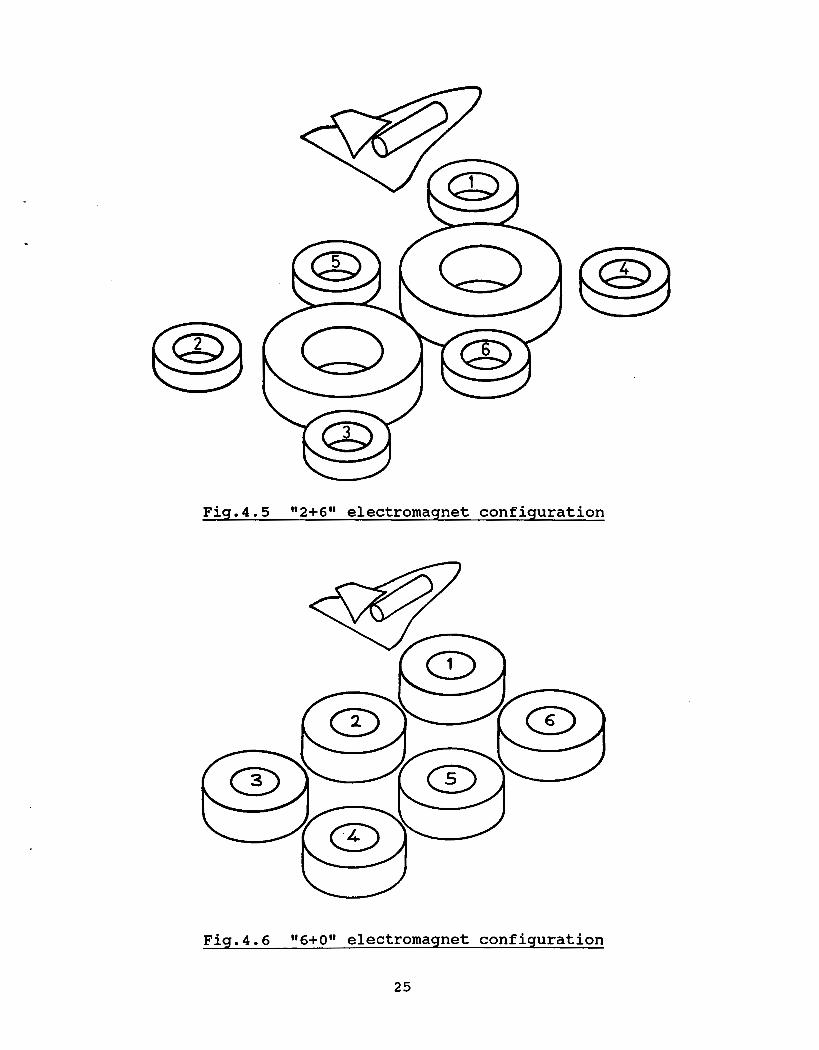
@ Fig.4 5 I12+6l1 electromagnet conf iquration

Fig.4.6 116+011 electromagnet configuration

25

5 FURTHER MAGNETIC DESIGN

5.1 Roll control

In model axes, several field or field gradient components are already primary producers of force or moment components :

Yaw moment Pitch moment

Axial force BZ Y B

Sideforce X y Vertical force

An effective roll moment technique would utilize some other

Bxx

Bxz

field or field gradient component so as to remain uncoupled, to a first order, from other degrees of freedom. The axial field component (Bx) cannot produce roll torque directly. The B w and

gradient components are intimately related to Bxx ( V . B = O ) .

gradient component was exploited in Ref.5 with the Bz z The B

Spanwise Magnet roll control scheme. This scheme involves the addition of magnetic cores magnetized largely in the spanwise direction and distributed symmetrically about the model's plane of symmetry (Fig. 5.1) . With the "2+6" electromagnet configuration, the required field gradient can be generated by the six control electromagnets, particularly effectively, in fact, by the central pair.

YZ

Current sense Geometry 5 6

5.2 Yaw angle requirement

The difficulties inherent in the "magnetic1' approach to this question have already been discussed. Detailed analysis would be a lengthy process and is quite beyond the scope of the report. However, modifications to the electromagnet configurations already studied can be anticipated. The "2+61' configuration can, it seems, be modified somewhat as shown in Fig.5.2, forming effectively two overlayed systems, offset at 90 degrees to each

26

other. It is expected that this arrangement would function satisfactorily around 0, 90, 180, 270 degrees yaw, but careful study of intermediate angles is required.

point levitation system could be mounted on a large turntable, with the axis of rotation vertical, and simply aligned mechanically in the desired yaw orientation. This would easily give 360 degree capability. Some small magnetic maneuvering capability would exist around each local datum orientation. There are several difficulties however :

There is a less elegant but workable alternative. A single

1) Electromagnet weight. A vague estimate of the weight of electromagnets, based on Section 4, would be around 15 tonnes (8 tonnes electromagnets, 7 tonnes support structure). This is not an unreasonably heavy assembly to move with precision; astronomical telescopes are surely of comparable weight.

2) Current leads and coolant lines. It is felt that careful design could accomodate the numerous high current supply leads to the electromagnets. These would be normally conducting where flexibility was required. Flexible helium transfer lines are technically feasible and are used in some applications, but tend to be expensive and delicate.

3) The location of the electromagnet assembly would have to be accurately monitored. This appears straightforward.

27

+

I

t z Fig.5.1 Spanwise magnet roll control

I i

Fig.5.2 112+611 electromagnet configurat

28

ton adapted for 360 degrees yaw

~ i

6 OPERATIONAL CONSIDERATIONS

6.1 Stray magnetic fields

This is an important issue is the choice of site for an ML facility. The system creates large regions of intense magnetic fields. There are known biological effects of steady magnetic fields, though the "safe" levels of exposure are ill-defined at present. Several nuclear physics experiments have been operated on the following guidelines (Ref . 13) :

Time Body area Field strength (Tesla/Gauss) o---------I----------~---~o-------------o------~o---------

Hours Whole body 0.02 / 200 Arms & hands 0.2 / 2000

Minutes Whole body 0.2 / 2000 Arms & hands 2 / 20,000

Several recent reports concerning biological effects of

Calculated magnetic field from a single optimized

magnetic fields have been discovered and have been added to the reference list.

electromagnet from Section 4.1.2 is shown in Fig.6.1. This shows that personnel would be excluded from the ML area during system operation. Since the loss of control of the levitated model is always a possibility (see Section 6.2) this may not be a serious restriction.

More troublesome could be the effect of weaker fields on sensitive equipment in the vicinity of the ML system. With the 13 inch MSBS, fields of the order of 1 Gauss have been shown to have an observable effect on standard CRT displays (picture distortion). A 1 Gauss field criteria would only be satisfied around 15/20 meters from the center of the single elctromagnet of Fig. 6 . 1. desirable. This would take the form of high permeability (steel, permalloy, mumetal) lining of an ML laboratory, such that the return flux paths would tend to be through the shielding rather than through outside air-paths. Careful calculation of the required shielding thickness and performance would be necessary.

Some form of magnetic shielding is possible, perhaps

6.2 Reliability

wind tunnel MSBSs. It had been considered that a Large MSBS would have to be very reliable, insofar as loss of control of a suspended model would have to be a very rare event. This is due to the fact that wind tunnel models tend to be expensive to construct, rather delicate and loss of control with wind on would inevitably result in the model being blown down the tunnel and damaged or destroyed. The difficulty in achieving high reliability with MSBSs arises because the inclusion of redundant hardware in the electromagnet array is expensive. Nevertheless,

Extensive consideration of this point has been devoted to

29

it had been concluded (Ref.5) that effective hardware redundancy could be achieved at reasonable cost, with careful design and operational techniques.

Reliability requirements for ML may be less severe. The lower loads and lower dynamic force capability imply that loss of control might be a less violent event than is sometimes the case with MSBSs. Rapid shutdown (current dump) of electromagnets would result in the model merely falling to the floor. If the model were robustly made and the floor were covered with some form of energy absorbing material, such an event might be perfectly acceptable.

c

30

\

1

4 8

CS6

H-33

I.c9 . \ %\ . \

Magnetic field strength in Gauss (0.0001 Tesla)

\

\

I

\

\ z\

\

I

I

\ a\

\ I I

Fig.6.1 Magnetic field strength distribution around sinale electromaanet

31

7 DISCUSSION

Calculations performed so far seem to confirm the technical feasibility of the demonstration Magnetic Levitation system. Electromagnet and power supply specifications appear quite reasonable. A key design choice, inviting an early decision, has been identified, relating to the problem of the yaw angle requirement :

a) The approach requires considerable design analysis at an early stage, but provides an elegant and versatile solution.

b) The %echanicalI1 approach is guaranteed to work but is somewhat inelegant and may represent no cost saving over a) above.

Whatever the choice, a comprehensive system simulation effort should be undertaken, in order to better identify certain design parameters, such as power supply voltage requirements.

All calculated electromagnet specifications should be regarded as preliminary. Considerable further analysis is required, particularly involving the effect of magnetic couplings and simultaneous provision of magnetic force and moment components. It is certain that substantial optimization is possible.

32

.

1.

2.

3.

4.

5.

6.

7.

8.

9.

10.

11.

12.

13 .

REFERENCES

Tuttle, M.H.; Kilgore, R.A.; Boyden, R.P.: Magnetic suspension and balance systems - a selected annotated bibliography. NASA TM-84661, July 1983.

Bloom, H.L. et al: Design concepts and cost studies for magnetic suspension and balance systems. NASA CR-165917, July 1982.

Boom, R.W.; Eyssa, Y.M.; McIntosh, G.E.; Abdelsalam. M.K.: 1/

Magnetic suspension and balance system study. NASA CR-3802, July 1984.

Boom, R.W.; Eyssa, Y.M.; McIntosh, G.E.; Abdelsalam, M.K.: Magnetic suspension and balance system advanced study. NASA CR-3927, October 1985.

Britcher, C.P.: Some aspects of magnetic suspension and balance systems with special application at large physical scales. NASA CR-172154, September 1983.

Britcher, C.P.; Goodyer, M.J.; Scurlock, R.G.; Wu, Y.Y.: A flying superconducting magnet and cryostat for magnetic suspension of wind-tunnel models. Cryogenics, April 1984.

Britcher, C.P.: User guide for the digital control system of the NASA Langley Research Center's 13-inch magnetic suspension and balance system. NASA CR-178210, March 1987.

LaFleur, S.S.: Advanced optical position sensors for magnetically suspended wind tunnel models. 11th International Congress on Instrumentation in Aerospace Simulation Facilities. Long Beach, CA, August 1985.

Covert, E.E.; Finston, M.; Vlajinac, M.; Stephens,T.: Magnetic suspension and balance systems for use with wind tunnels. Progress in Aerospace Sciences, Vo1.14, 1973

Stephens, T.; Design, construction and evaluation of a magnetic suspension and balance system for wind tunnels. NASA CR-66903, November 1969.

Goodyer, M.J.: The magnetic suspension of wind tunnel models for dynamic testing. University of Southampton PhD thesis, April 1968.

Grover, F.W.: Inductance calculations, working formulae and tables. Van Nostrand, 1946.

Ketchen, E.E.; Porter, W.E.; Bolton, N.E.: The biological effects of magnetic fields on man. Journal of the American Industrial Hygiene Association, January 1978.

33

Additional references relating to biological effects of magnetic fields :

14. American Institute of Biological Sciences: Biological and human health effects of extremely low frequency electromagnetic fields. Report ADA-152731, March 1985.

15. Polk, C.; Postow, E.: Biological effects of magnetic fields on man. CRC Handbook series. CRC Press. 1986.

.

34

APPENDIX 1

The computer program FORCE (Ref.5) was developed from the MIT program TABLE, specifically for the purpose of analysis of electromagnet geometries for MSBSs. Arrays of air-cored electromagnets are represented by straight line conductor segments and magnetic fields can then be calculated by summation of the effect of each segment, by repetitive use of the Biot- Savart law. If the magnetization of the model cores is known (permanent magnets) then these cores can be represented as arrays of magnetic dipoles. Forces and moments can now be found by calculating the magnetic field and field gradient components, due to the external electromagnets, at each dipole and summing these elemental forces and moments over the whole model.

The accuracy of these methods is adequate for most MSBS/ML design purposes, but is dependent on the level of discretization of electromagnet and model cores. The serious shortcomings of FORCE are the lack of graphical 1/0 and the inability to handle iron electromagnet or model cores.

A few programs designed to handle the non-linear problems of iron cores do exist. Notable amongst these are GFUN and TOSCA. GFUN relies on an integral technique and has been successfully used for MSBS rolling moment calculations (Ref.5). TOSCA uses a differential equation method. Each program has its own advantages and disadvantages, but both are very sophisticated and require considerable care in operation, though are capable of quite accurate results.

35

1. Report No. 2. Government Accession No.

NASA CR- 178301 4. Title and Subtitle

Technical Background for a Demonstration Magnetic Levitation System

3. Recipient's Catalog No.

5. Repon Date

I

7. Author(sj 8. Parforming Organization Report No.

Colin P. Britcher

9. Performing Organization Name and Address Old Dominion University Department of Mechanical Engineering and Mechanics Norfolk, VA 23508

12. Sponsoring Agency Name and Address

10. Work Unit No.

I 505-6 1-9 1-0 1 11. Contract or Grant No.

NAG1-7 16 13. Type of Report and Period Covered

Contractor Report National Aeronautics and Space Administration Washington, DC 20546-0001

17. Key Words (Suggested by Author($) )

Magnetic Levitat ion Magnetic Suspension

14. Sponsoring Agmcy coda

18. Distribution Statement

Unclassified - Unlimited

I

15. Supplementary Notes

Technical Monitor: Richmond P. Boyden, NASA Langley Research Center, Hampton, Virginis

19. Security aaoif . (of this report)

Unclassified

16. Abstract

20. Security Classif. (of this page) ' 21. NO. of P- 22. Price

Unclassified 37 A0 3

A preliminary technical assessment of the feasibility of a demonstration Magnetic Levitation system, required to support aerodynamic models with a specified clear air volume around them, is presented. Preliminary calculations of required sizes of electromagnets and power supplies are made, indicating that the system is practical. Other aspects,including model position sensing and controller design, are briefly addressed.