Embed Size (px)
Citation preview

Food Processing Concepts
for Entrepreneurs and
Small-Scale Processors
Donald G. Mercer, Ph.D., P.Eng., FIAFoST
Department of Food Science
University of Guelph
© 2018

The material presented here has been copyrighted as a
means of protecting this body of work. It is not my intention
to impose any restrictions on the printing, copying, or
distribution of this information. If you find any of the chapters
useful for your food processing activities, or if you would like
to use anything for instructional purposes, please feel free to
do so. A reference citing the source of any material which is
reproduced would be greatly appreciated, whenever it is used.
As author, I assume no responsibility, nor liability, for any
problems of any nature or manner which may be encountered
through the application of the principles discussed here. Your
processing equipment, starting materials, and individual
applications will almost certainly impose conditions that will
create unique situations. These cannot be anticipated in a
general context such as that presented here.
© Donald G. Mercer
April 2018
ISBN 978-0-88955-650-8
269 pages - 266 figures - 15 tables

To Our Grandchildren
Ethan, Mataya, Keeleigh, and Arison

Table of Contents Page i
FOOD PROCESSING CONCEPTS
FOR ENTREPRENEURS AND SMALL-SCALE PROCESSORS
TABLE OF CONTENTS
Chapter 1: Introductory Comments
1.1 Personal Background 1.2 Lessons Learned 1.3 Using This Guide 1.4 Photographs, Diagrams, and Tables 1.5 Some Words of Appreciation
Chapter 2: Why Food Is Processed
2.1 General Reasons for Processing 2.2 Food Quality 2.3 Food Safety 2.4 Deterioration 2.4.1 Physical Deterioration 2.4.2 Chemical Deterioration 2.4.3 Biological Deterioration 2.4.4 Time 2.5 Contamination 2.5.1 Physical Contamination 2.5.2 Chemical Contamination 2.5.3 Biological Contamination 2.5.4 Allergens 2.6 Summary Comments 2.7 References
Chapter 3: Historical Development of Food Processing 3.1 Introduction 3.2 Early Advances in Food Processing 3.3 Advances by Louis Pasteur 3.4 Modern Advances in Food Processing 3.5 References

Table of Contents Page ii
Chapter 4: Background Skills for Food Processing 4.1 Introduction 4.2 Organizing Information 4.3 Dimensional Analysis 4.3.1 Practice Problems – Dimensional Analysis 4.4 Temperature 4.4.1 Practice Problems – Temperature 4.5 Pressure 4.5.1 Practice Problems – Pressure 4.6 Density and Specific Gravity 4.6.1 Determining Densities of Liquids 4.6.2 Determining Densities of Solids 4.6.3 Practice Problems – Density and Specific Gravity 4.7 Mass Balances 4.7.1 Practice Problems – Mass Balances 4.8 References Chapter 5: Heating and Cooling in Food Processing 5.1 Introduction 5.2 Changes of State 5.3 Specific Heat 5.4 Latent Heat 5.5 Calculations of Heat Addition and Removal 5.5.1 Heating of Frozen Products – Sample Calculations 5.5.2 Freezing of Products – Sample Calculations 5.5.3 Practice Problems 5.6 Steam as a Heat Source 5.6.1 Sample Steam Calculations 5.7 Heat Balances 5.7.1 Practice Problems 5.8 References

Table of Contents Page iii
Chapter 6: Thermal Processing Basics 6.1 Introduction 6.2 Definitions 6.3 Heat Transfer Mechanisms 6.4 Pasteurization and Blanching 6.5 Pasteurization and the Thermal Processing of Milk 6.5.1 Indicator Enzymes in Milk Pasteurization 6.6 Batch and Continuous Thermal Processes 6.6.1 Effects of Particle Size on Heat-up Time of Solids 6.7 Equipment Used in Heating and Cooling 6.7.1 Jacketed Kettles 6.7.2 Plate Heat Exchangers 6.7.3 Tubular Heat Exchangers 6.7.4 Scraped Surface Heat Exchangers 6.7.5 Shell and Tube Heat Exchangers 6.8 Cleaning and Fouling 6.9 Summary Comments 6.10 References Chapter 7: Thermal Processing – Specialized Calculations 7.1 Introduction 7.2 Holding Times 7.2.1 Holding Time Calculations 7.2.2 Tests for Retention Time 7.2.3 Tube and Pipe Diameters 7.2.4 Calculations Involving Tube and Pipe Diameters 7.3 Thermal Destruction of Microorganisms 7.4 Decimal Reduction Time 7.5 Sample Microbial Death Calculations 7.6 Sterilization Criteria 7.7 Thermal Resistance Constant (“Z” Values) 7.8 Thermal Death Time (“F” Values) 7.9 Safety Margins 7.10 Spoilage Probability 7.11 Process Lethality 7.12 Calculation of F Values at Different Temperatures 7.13 An Alternate Way of Looking at Z Values 7.14 References
Table of Contents Page iv
Chapter 8: Basics of Drying Food Materials 8.1 Introduction 8.2 Reasons for Drying Food Products 8.3 Historical Development of Food Drying 8.4 Wet and Dry Basis Moistures 8.4.1 Sample Calculations 8.4.2 Moisture Calculation Case Study 8.4.3 Comparing Moisture Contents 8.5 Explaining the Mechanisms of Drying 8.6 Factors Influencing Drying 8.6.1 Product-Related Attributes 8.6.2 Dryer-Related Attributes 8.7 Impact of Drying on the Product 8.8 Continuous Through-Circulation “Belt” Dryers 8.9 Other Types of Dryers: How They Operate and Their Applications 8.10 Dryer Water Removal Capacity 8.11 Osmotic Dehydration 8.12 Sample Calculations 8.13 Practice Problems 8.14 Specialized Drying Calculations 8.15 References

Table of Contents Page v
Chapter 9: Chilling and Freezing 9.1 Introduction 9.2 What is Chilling? 9.3 How Does Chilling Differ from Freezing? 9.4 Why Do We Chill Food? 9.5 How Do We Chill Food? 9.6 Perishability 9.7 Effects of Chilling on Microbial Growth 9.7.1 Introduction 9.7.2 Storage Temperatures 9.7.3 Temperature Limits for Growth 9.7.4 Phases of Growth 9.8 Enzyme Activity in Stored Foods 9.9 Effects of Chilling on the Respiration of Foods 9.9.1 Introduction 9.9.2 Respiration in Fruits and Vegetables 9.9.3 Controlled Atmosphere Packaging 9.9.4 Respiration Rates of Various Fruits and Vegetables 9.10 Climacteric Ripening 9.10.1 What Is Climacteric Ripening? 9.10.2 Applications of Climacteric Ripening 9.11 Other Factors in the Chilling of Fruits and Vegetables 9.11.1 Introduction 9.11.2 Reduction of Moisture and Volatile Losses 9.11.3 Avoiding Moisture Loss 9.12 Chilling Injury 9.13 Storing Potatoes 9.14 Storing Bread Products 9.15 Freezing Fruits and Vegetables 9.15.1 Introduction 9.15.2 Freezing Points of Liquid and Solid Foods 9.15.3 Volume Changes on Freezing 9.16 Ice Crystal Formation During Freezing 9.16.1 Background 9.16.2 Freezing of Pure Water 9.16.3 Freezing of Sugar Solutions and Jam 9.16.4 Thawing of Water (Ice) and Strawberry Jam 9.16.5 Effect of Ice Crystal Growth on Frozen Products 9.16.6 Ice Crystal Growth During Storage 9.17 Calculation of Freezing Times 9.18 Summary Comments 9.19 References
Table of Contents Page vi
Chapter 10: Separation and Concentration 10.1 Introduction 10.2 Membrane Filtration 10.2.1 Terminology 10.2.2 Methods of Operation 10.2.3 System Characteristics 10.2.4 Reverse Osmosis 10.2.5 Comparison of Membrane Filtration Techniques 10.2.6 Concentration and Volume Reduction Factors 10.2.7 Sample Calculation 10-1 10.2.8 Applications of Membrane Separation Processes 10.3 Freeze Concentration 10.3.1 Sample Calculation 10-2 10.4 Centrifugation 10.5 Evaporation 10.6 Ion Exchange 10.6.1 Basic Principles 10.6.2 Sodium Ions in Solution 10.6.3 Regeneration of Ion Exchange Resins 10.6.4 Food-Related Applications of Ion Exchange 10.7 Adsorption 10.8 Chromatographic Techniques 10.8.1 Basic Principles 10.9 Solvent Extraction 10.10 Supercritical Fluid Extraction 10.11 Precipitation 10.11.1 Basic Principles 10.11.2 Protein Recovery by Precipitation 10.12 Summary Comments 10.13 References Chapter 11: Closing Comments Chapter 12: List of Figures and Tables

Chapter 1: Introductory Comments Page 1 - 1
1. Introductory Comments 1.1 Personal Background Food processing has been an important part of my life for over forty years. After finishing university, I was fortunate to spend a post-doctoral year with a major international food company (General Foods) at their Research Department in Cobourg, Ontario. During a total of fourteen years with the company which later became Kraft-General Foods, I had the pleasure of working on a variety of projects including process modelling and optimization; process design and commissioning; product drying; aseptic packaging; and a number of other activities. This was like a dream job for a Chemical Engineer with my particular interests. With the closure of the Canadian Research Department, I moved to Agriculture and Agri-Food Canada (AAFC) on the Central Experimental Farm in Ottawa where I was a “Special Advisor on Food” and later a “Commercialization Officer”. The positions there allowed me to see a different side of the agri-food sector, which was entirely new to me. Half-way through my ten years with Agriculture and Agri-Food Canada, I was transferred to the newly established Guelph Food Research Centre. Soon after this, I was seconded to the Department of Food Science at the University of Guelph where I taught Food Processing courses from 1997 to 2003. In 2003, I joined the Department of Food Science on a full-time basis and
things have progressed steadily from there. Over the past fifteen years as a faculty member, I have spent considerable time working with small and medium sized enterprises – SME’s in the popular jargon. I began my international activities investigating processing opportunities for tomatoes and other products in Equatorial Guinea and Honduras. These focussed on solar drying and techniques that were not highly reliant on electricity as an energy source. Another project found me identifying the challenges facing the agri-food sector in Malawi as well as designing and building a dryer for mangoes at Bunda College in Lilongwe. Later, I found myself working on projects in Tanzania to increase the capacity for technology transfer by setting up courses at Kihonda College in Morogoro. These activities began to expand to include the development of food processing courses for St. Vincent and the Grenadines Community College and working with Dominica Community College. In 2015, I started working with the Inter-American Institute for Cooperation on Agriculture (IICA) to offer training courses on mango processing in St. Kitts and Nevis. This continued with subsequent workshops in 2016 in St. Kitts and Nevis, as well as in Antigua and Barbuda. Future workshops are planned for St. Lucia and Grenada in 2018. One of my most enjoyable activities has been working with the International Academy of Food Science and Technology (IAFoST) as Vice-Chair of

Chapter 1: Introductory Comments Page 1 - 2
the Distance Assisted Training Program. This program, under the admirable leadership of Dr. Daryl Lund (Professor Emeritus, University of Wisconsin – Madison) is directed at providing training in thirteen key areas of Food Science to food industry workers. Through IAFoST, I have been able to participate in Food Science training workshops in Brazil, Myanmar, Vietnam, and Kenya. These experiences have allowed me to become familiar with a number of the challenges facing food processors in different countries. This is especially true in the case of small-scale processors and entrepreneurs. 1.2 Lessons Learned During my international activities, it became increasingly apparent that the small and medium enterprises and entrepreneurs involved in food processing were greatly under-served when it came to providing them with information. Much of what university researchers do is geared to academic publications in technical journals. Such efforts are totally understandable and absolutely essential for the continued advancement of intellectual knowledge, and an understanding of basic scientific principles. Without this research, advances in Food Science would suffer tremendously. However, there has not been as much emphasis placed on delivering instructional material to the small-scale food processors and entrepreneurs who
need and want information on how to perform basic processing operations. There is not enough resource material available to them on food-related cause-and-effect relationships. Nor are many of the existing sources of information presented in a format that can be readily transferred into practice by someone who is faced with the challenge of preparing a high quality product that is safe for consumers. While working with groups of twenty to thirty small-scale processors, the need for such resource material became abundantly clear. That was the impetus for putting together this guide to food processing. 1.3 Using This Guide One of the phrases that I find myself using quite frequently is “One size fits none.” This is usually associated with clothing where the makers claim that their product will fit a wide range of people, with the end result that it fits no one all that well. Putting together a guide to food processing is essentially the same type of thing. No single body of work can address the needs of everyone. No matter what is included, something will be left out that a particular group feels is imperative to have included. Other readers will question why a certain topic was included when they see no relevance to it at all. This guide cannot be all things to all readers, and I fully recognize this fact. In putting together this reference source, I looked at the basic technologies employed in food processing. The next step was to expand on them in order to

Chapter 1: Introductory Comments Page 1 - 3
provide insight into the reasons for processing food, and how we do this. These are the fundamentals without which you cannot approach food processing in an informed manner. When reading through the following chapters, you may find that the mathematical treatments of such things as drying become overly involved for what you really need to know. If this is the case, then simply skip these parts and take away the information that you need to approach your activities and, hopefully, solve the problems you are facing. Mathematics is something that cannot be avoided in food processing applications. We use math to put together recipes and product formulations. We may need to calculate moisture contents and processing yields. There can be times when we require heat calculations. The list just goes on and on. I have tried whenever and wherever possible to include sample calculations to guide you through some of the scenarios that you may typically encounter. Case studies have also been included in hope of illustrating some of the situations faced by food processors. While these are based on actual real-life experiences, I have had to alter the details due to confidentiality concerns. If you require a more in-depth treatment of various aspects of a food processing technique, this guide will introduce you to the topic and allow you to move on to more technical or more academically-oriented sources. To those who feel that I have included too much – I apologize. To those who
feel that certain essentials are missing – I also apologize. The material presented here is for instructional purposes only. As the author, I cannot assume any responsibility, nor liability, for problems which may be encountered as a result of anyone attempting to use the information presented here. Your starting materials, equipment, and individual applications will almost certainly impose conditions that will create unique situations. These cannot be anticipated in a general context such as that presented here. If there are any doubts regarding the safety or suitability of your products for human (or even non-human) consumption, you should consult the proper authorities, or work with reputable, qualified equipment suppliers. You also need to keep in mind that regulations pertaining to food processing and distribution are established and enforced by various organizations in different jurisdictions. It is crucial that you obey the laws in place within the areas where you are manufacturing and/or marketing your product. If you are exporting your product to be sold in a foreign country, it is frequently the case that you must obey the regulations in force within the country where the product will be sold, rather than those rules in force within your own country. Failure to recognize this may result in your product being refused entry into an export market and returned to you at your expense. Material presented here has been copyrighted as a means of protecting this body of work. It is not my intention to impose any restrictions on the

Chapter 1: Introductory Comments Page 1 - 4
printing, copying, or distribution of this information. If you find any of the chapters useful for your processing activities, or if you would like to use anything for instructional purposes, please feel free to do so. A reference citing the source of any material which is reproduced would be appreciated, whenever it is used. 1.4 Photographs, Diagrams, and Tables All photographs appearing in the following chapters were taken by the author and are subject to copyright considerations. This is also true of the diagrams. On occasion, diagrams have been patterned after works by others. In these cases, the source of the original information has been acknowledged. All tables are the work of the author. Throughout this guide, I have drawn heavily upon personal experiences. As a result, any and all errors that may have crept into these pages are entirely my own. 1.5 Some Words of Appreciation All too often, we take for granted the support of those around us. As I look upon the number of hours that have gone into putting together this “Food Processing Concepts for Entrepreneurs and Small-Scale Food Processors”, I am certainly appreciative of the support of my family members. They are the ones who are always there, and I need to thank them publicly. The patience and understanding of my wife, Jane, has helped to make this all
possible. When I was doing a lot of the drying projects, she was the one who put up with my long days in the lab, going into work on weekends, and doing “number crunching” in the evenings for the mathematical modelling activities. She’s the one who humoured my building dryers in our garage, and setting up solar dryers in the backyard. Fortunately, Jane has been doing some writing of her own, so she understands the time and effort that goes into putting our ideas down on paper. I would also like to acknowledge our other family members: our son Darren and his wife Karren (yes, I know, they rhyme!), our son Geoffrey and his wife Maren, and our daughters Andrea and Destiny. There are four very special family members to whom I wish to dedicate this work - our four grandchildren; Ethan, Mataya, Keeleigh, and Arison. Of all the important things in this world, there is none so important as family. I would like to recognize my father, Tom Mercer, and my late mother, Audrey, who were always so supportive in all of my endeavours. It is my sincere hope that you find the information presented here useful for your particular needs and applications, and I wish you every success in your food processing activities. It’s a lot of work, but it can be extremely rewarding. Sincerely, Donald G. Mercer, Ph.D., P.Eng., FIAFoST April 6, 2018.

Chapter 2: Why Food is Processed Page 2 - 1
2. Why Food Is Processed 2.1 General Reasons for Processing At first glance, the reasons why food is processed may seem obvious to some. It is often considered that food products are processed solely to extend their storage life or to reduce the risk of spoilage (Figure 2-1). However, there are additional reasons why foods are processed.
Figure 2-1: Avoiding microbial spoilage is a major reason foods are processed.
It has been estimated by various sources that one-third to one-half of the world’s food supply is lost due to spoilage (Figure 2-2). Food losses in the United States of America have been estimated to be as high as 40% (Gunders, 2012).
Figure 2-2: One-third to one-half of the world’s food supply is lost due to spoilage.
Essentially, the quest to extend the storage life or “shelf-life” of a food product stems from a need to match supplies of food with the demands of time and space, or location.
In countries like Canada and the northern portions of the United States, the ability to grow food products is limited by the climatic conditions characterized by the four seasons of the year. During an appreciable portion of the year, it is too cold to grow crops. This means that crops harvested in the late summer or early fall must be maintained in a quality form for use throughout the winter and spring months until fresh produce can be obtained during the following year’s growing season. Food processing allows these time-related needs to be addressed. Apart from the growing season considerations, many consumers want foods that will simply last for a long time when stored in their pantries, on their kitchen shelves, or in their freezers. By processing foods such as fruits and vegetables when they are at their peak of quality and freshness, food processors can deliver products to meet these demands (Figures 2-3a and 2-3b).
Figure 2-3a: Processing permits use of foods in the off-season.
Figure 2-3b: Processing extends product shelf-life.

Chapter 2: Why Food is Processed Page 2 - 2
While certain areas of the world are enduring months of harsh climates, other portions of the world are enjoying much more temperate conditions. These countries may be able to harvest crops continuously, or may be able to grow two crops per year. By exporting agricultural commodities, many tropical countries are able to sell their produce to an enthusiastic market willing to pay higher prices for fresh produce during the “off season”. Food processing often plays a role in getting this food from one location to another while minimizing the loss of quality and nutrition, thereby addressing what we might describe as “space-related needs” (Figure 2-4).
Figure 2-4: Processing permits transportation of food materials over distances and time.
Many of the things that are taken for granted during the winter months, including fresh tropical fruits, were not available prior to the end of World War II. It was not until controlled supply chains were developed to get these products from their source to waiting markets that the potential for exports could be fully exploited. Unfortunately, there are areas of the world that cannot produce enough food
to feed their own populations during any portion of the year. Through drought or the encroachment of desert landscapes, there is not the water nor the soil fertility to produce sufficient amounts of food. At the same time, more distant nations may be enjoying bumper harvests and actually be experiencing food surpluses that go well beyond their foreseeable future needs. If these foods could be shipped to the areas in such dire distress, in a readily utilizable form that would be stable over time, both the spatial and time-related needs could be met. Fortunately, this is within the realm of possibility through the application of food processing technology. Food processing also helps to ensure the cleanliness, and safety of the world’s food supply. Through the application of food processing, it is possible to reduce levels of microbial contamination that would otherwise create outbreaks of disease that could afflict millions. Simply washing fruits and vegetables in clean, “potable” (i.e., drinkable) water is a good first step in any processing procedure (Figure 2-5).
Figure 2-5: Washing is an important first step in processing.
Chapter 2: Why Food is Processed Page 2 - 3
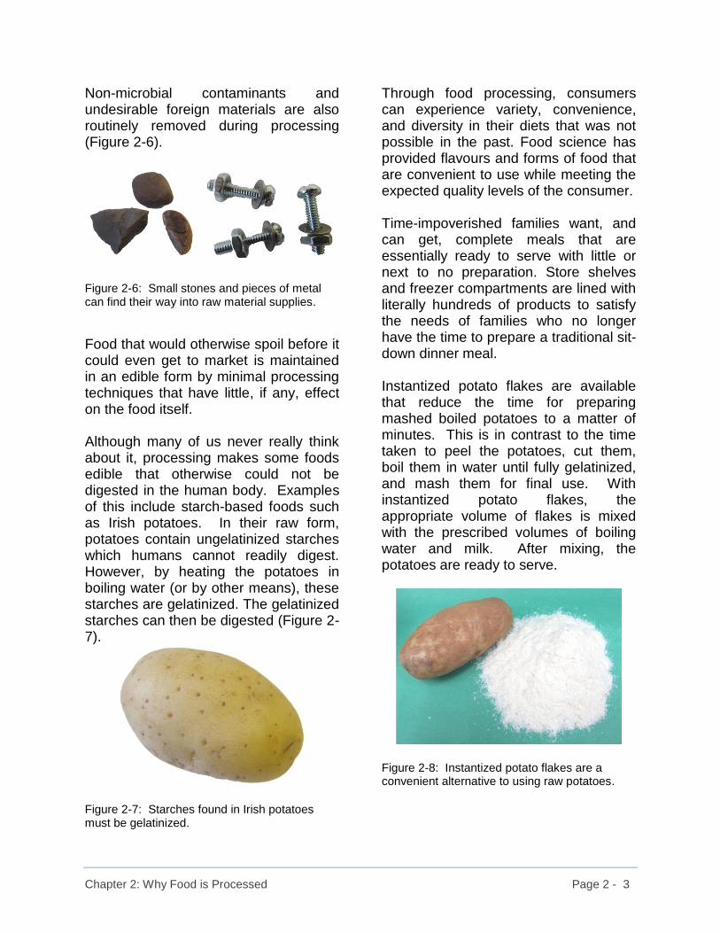
Non-microbial contaminants and undesirable foreign materials are also routinely removed during processing (Figure 2-6).
Figure 2-6: Small stones and pieces of metal can find their way into raw material supplies.
Food that would otherwise spoil before it could even get to market is maintained in an edible form by minimal processing techniques that have little, if any, effect on the food itself. Although many of us never really think about it, processing makes some foods edible that otherwise could not be digested in the human body. Examples of this include starch-based foods such as Irish potatoes. In their raw form, potatoes contain ungelatinized starches which humans cannot readily digest. However, by heating the potatoes in boiling water (or by other means), these starches are gelatinized. The gelatinized starches can then be digested (Figure 2-7).
Figure 2-7: Starches found in Irish potatoes must be gelatinized.
Through food processing, consumers can experience variety, convenience, and diversity in their diets that was not possible in the past. Food science has provided flavours and forms of food that are convenient to use while meeting the expected quality levels of the consumer. Time-impoverished families want, and can get, complete meals that are essentially ready to serve with little or next to no preparation. Store shelves and freezer compartments are lined with literally hundreds of products to satisfy the needs of families who no longer have the time to prepare a traditional sit-down dinner meal. Instantized potato flakes are available that reduce the time for preparing mashed boiled potatoes to a matter of minutes. This is in contrast to the time taken to peel the potatoes, cut them, boil them in water until fully gelatinized, and mash them for final use. With instantized potato flakes, the appropriate volume of flakes is mixed with the prescribed volumes of boiling water and milk. After mixing, the potatoes are ready to serve.
Figure 2-8: Instantized potato flakes are a convenient alternative to using raw potatoes.

Chapter 2: Why Food is Processed Page 2 - 4
Microwavable meals or ready-to-eat meals from in-store delicatessens cater to these individuals and families (Figure 2-9).
Figure 2-9: Microwavable meals offer variety and convenience (frozen on left, heated on right)
A diversity of ethnic dishes that was unknown to preceding generations can now be enjoyed by today’s consumer. As communications, world travel, and immigration have increased, so has the appreciation of the fine foods that are available in what were previously considered to be exotic locations. Food processing has brought the production of many “ethnic” foods to countries where they have now become favorites. Not only that, but they are available in convenient formats which may only require thawing and heating.
2.2 Food Quality Food quality has already been mentioned several times. However, the attributes which go together to create an overall impression of quality have not been fully articulated. It is important not to confuse “quality” with “safety”. Although the terms are often used interchangeably, their actual meanings are quite different. We will discuss “food safety” in the next section. The following are some of the factors used to define food quality: • Nutritional value • Aesthetic aspects: • appearance / colour • taste / flavour • feel / texture • aroma
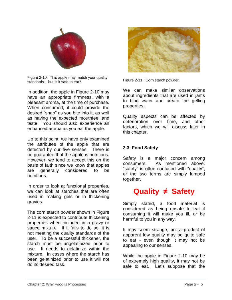
• sound • etc. • Functional properties: • gelation properties • thickening properties • water binding ability The typical consumer most frequently judges quality on the aesthetic aspects which appeal to the five senses. If a product doesn’t look appealing the consumer will reject it. If you envision an apple, you will have some pre-conceived ideas as to what it should look like. It should have a certain shape and colour as well as being free from blemishes. The apple shown in Figure 2-10 has a pleasing red colour, a characteristic shape for this variety, and the peel is not marked.
Chapter 2: Why Food is Processed Page 2 - 5
Figure 2-10: This apple may match your quality standards – but is it safe to eat?
In addition, the apple in Figure 2-10 may have an appropriate firmness, with a pleasant aroma, at the time of purchase. When consumed, it could provide the desired “snap” as you bite into it, as well as having the expected mouthfeel and taste. You should also experience an enhanced aroma as you eat the apple. Up to this point, we have only examined the attributes of the apple that are detected by our five senses. There is no guarantee that the apple is nutritious. However, we tend to accept this on the basis of faith since we know that apples are generally considered to be nutritious. In order to look at functional properties, we can look at starches that are often used in making gels or in thickening gravies. The corn starch powder shown in Figure 2-11 is expected to contribute thickening properties when included in a gravy or sauce mixture. If it fails to do so, it is not meeting the quality standards of the user. To be a successful thickener, the starch must be ungelatinized prior to use. It needs to gelatinize within the mixture. In cases where the starch has been gelatinized prior to use it will not do its desired task.
Figure 2-11: Corn starch powder.
We can make similar observations about ingredients that are used in jams to bind water and create the gelling properties. Quality aspects can be affected by deterioration over time, and other factors, which we will discuss later in this chapter. 2.3 Food Safety Safety is a major concern among consumers. As mentioned above, “safety” is often confused with “quality”, or the two terms are simply lumped together.
Quality ≠ Safety Simply stated, a food material is considered as being unsafe to eat if consuming it will make you ill, or be harmful to you in any way. It may seem strange, but a product of apparent low quality may be quite safe to eat - even though it may not be appealing to our senses. While the apple in Figure 2-10 may be of extremely high quality, it may not be safe to eat. Let’s suppose that the
Chapter 2: Why Food is Processed Page 2 - 6
apple fell to the ground in the orchard while workers were picking them. There may have been cattle, goats, or other animals grazing under the apple trees prior to the harvesting. Grazing animals tend to leave their droppings behind which are contaminated with potentially harmful microorganisms. Microorganisms could be transferred to the surface of the fallen apple due to brief contact with contaminants on the ground. If the apple was not properly washed prior to eating, the consumer could end up suffering from serious health issues. In contrast, a less attractive apple could be totally safe to eat, yet not have all the apparent higher quality attributes. We will discuss food contamination later in this chapter. 2.4 Deterioration It is generally accepted that when any crop is harvested, or any product is manufactured, deterioration will begin almost immediately. While some degree of “aging” may enhance the quality of certain products such as wine or cheese, excessive or improper aging may render others useless. Most often, deterioration affects the quality of the food, but it can also have an impact on safety. In order to reduce or eliminate the effects of deterioration over time, it is necessary to understand the basic causes of this undesirable process. There are three basic methods by which food deterioration can occur.
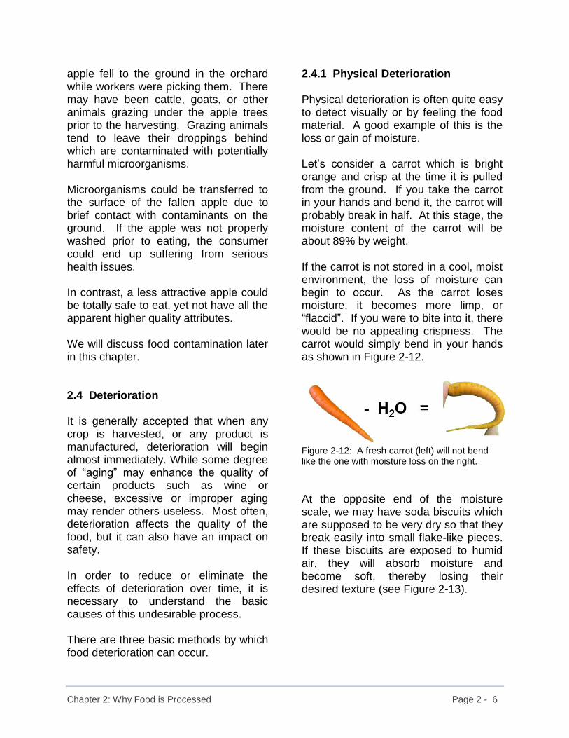
2.4.1 Physical Deterioration Physical deterioration is often quite easy to detect visually or by feeling the food material. A good example of this is the loss or gain of moisture. Let’s consider a carrot which is bright orange and crisp at the time it is pulled from the ground. If you take the carrot in your hands and bend it, the carrot will probably break in half. At this stage, the moisture content of the carrot will be about 89% by weight. If the carrot is not stored in a cool, moist environment, the loss of moisture can begin to occur. As the carrot loses moisture, it becomes more limp, or “flaccid”. If you were to bite into it, there would be no appealing crispness. The carrot would simply bend in your hands as shown in Figure 2-12.
Figure 2-12: A fresh carrot (left) will not bend like the one with moisture loss on the right.
At the opposite end of the moisture scale, we may have soda biscuits which are supposed to be very dry so that they break easily into small flake-like pieces. If these biscuits are exposed to humid air, they will absorb moisture and become soft, thereby losing their desired texture (see Figure 2-13).

Chapter 2: Why Food is Processed Page 2 - 7
Figure 2-13: The soda biscuit on the right has lost its crispness due to the uptake of moisture.
Another example of physical deterioration is the reduction of particle size or breakage of products. This can occur during transportation where the product may be subjected to vibrations and bumping on rough roads. In Figure 2-14, a biscuit is shown in its broken state.
Figure 2-14: Breakage is an example of physical degradation.
2.4.2 Chemical Deterioration As its description implies, chemical deterioration is the result of undesirable chemical reactions occurring within a food material. One of the most common degradation reactions is with oxygen. There is approximately 20% oxygen in the air around us, so it is quite natural that it would enter into reactions with compounds present in the food.
The juices of citrus fruit such as oranges contain delicate flavour oils that provide a pleasant aroma and taste. If these oils react with oxygen, they can produce unappealing off-flavours and a brown discolouration (Figure 2-15).
Figure 2-15: Aromatic oils in orange juice are susceptible to reactions with oxygen.
Another example of oxygen causing the deterioration of a product is oxidative rancidity. In this case, oxygen reacts with fats or oils to create a noticeable off-flavour. This is particularly common when butter or cooking oil is left exposed to the air for prolonged periods of time (Figure 2-16).
Figure 2-16: Butter (shown here) and vegetable oils may experience oxidative rancidity when exposed to air.
Many chemical and biological reactions speed up with increases in temperature. Based on an equation developed by the physical chemist Svante Arrhenius in 1889, it is generally accepted that the rate of a chemical reaction will double if

Chapter 2: Why Food is Processed Page 2 - 8
the temperature is increased from 10°C to 20°C. While this may not be exactly true for all reactions, it does provide a good indication of the effects of temperature on how fast a reaction can proceed. Using the opposite approach, it can be stated that the rate of a chemical reaction can be reduced by half if the temperature is lowered from 20°C down to 10°C. The energy present in sunlight can change the chemical structure of compounds present in food materials. Some light-sensitive products are sold in brown bottles to protect the contents from the negative effects of sunlight. If you have ever doubted the ability of sunlight to create chemical changes, take a look at the colour of fabrics, such as window curtains, exposed to the sun for prolonged time periods. You may also notice that their texture has changed and that the fabric no longer holds together very well. Even something as simple as a piece of newspaper can turn from white to a yellowish-brown due to prolonged exposure to sunlight
2.4.3 Biological Deterioration Some degree of care must be taken so as not to confuse biological deterioration with biological spoilage, which will be discussed later in this chapter. In addition, there may be some degradative chemical reactions that are caused by biological processes. One biological reaction that causes deterioration of quality involves the enzyme polyphenol oxidase. This reaction is particularly evident in cauliflower. Originally, the cauliflower florets are creamy-white in colour. However, with the passage of time, the naturally-occurring polyphenol oxidase present in the cauliflower can cause the development of brown, or even black, pigments. Figure 2-17 shows a fresh cauliflower and what it looks like after sitting at room temperature for approximately one week.
Figure 2-17: Changes in colour of a cauliflower due to polyphenol oxidase.
The growth of microorganisms is most often associated with contamination and disease.

Chapter 2: Why Food is Processed Page 2 - 9
2.4.4 Time Deterioration is what we call a “kinetic process”. This means that time plays a major role in many aspects of deterioration (Figure 2-18). It is a factor that must never be forgotten.
Figure 2-18: Time is a factor that can never be forgotten when dealing with food materials.
As a result, processors must minimize the time interval between the harvesting of a crop and its processing. With many perishable foods, or semi-perishable foods, the time interval between their processing and consumption is also important. Food processors must understand these food deterioration mechanisms and be able to address them through the application of appropriate processing techniques. While it is essential that any process reduce or eliminate causes of deterioration, these same techniques must not create additional issues of safety or quality loss.
2.5 Contamination A simple way of looking at a contaminant is to consider it as being anything that should not be present in a food product. Even something that is generally recognized as safe (i.e., it has ‘GRAS’ status) can be a contaminant if it should not be in the product formulation. This is because it will not appear on the ingredient line of that product and may possibly cause harm to an unsuspecting consumer. 2.5.1 Physical Contamination Physical contaminants are most often regarded as pieces of material that should not be present. These include things like small stones and pieces of metal as shown previously in Figure 2-6. Depending on their size, physical contaminants can be removed by screening the incoming raw materials. Metal detectors can be used to detect the presence of small pieces of metal. Dirt or soil clinging to the surfaces of fruits and vegetables is a very common contaminant (Figure 2-19). Fortunately, in most cases, it is relatively easy to remove.
Figure 2-19: Dirt trapped between the stalks of celery is an example of a physical contaminant.

Chapter 2: Why Food is Processed Page 2 - 10
The most problematic physical contaminant is broken glass (Figure 2-20). It is extremely hard to see and there are no simple methods available for detecting its presence in food products. For this reason, glass should be banned from all production areas, with the possible exception of the final packaging line where glass bottles may be the desired form of containment.
Figure 2-20: Broken glass is a serious physical contaminant.
2.5.2 Chemical Contamination Contamination of food materials by various chemicals can happen along the entire food production continuum. Pesticide and herbicide residues used for killing insects and weeds before the time of harvest can remain in the food and pose a health danger to consumers. Improper storage and handling of such things as fertilizers on the farm, or chemicals in production facilities can lead to contamination of food products after harvesting (Figure 2-21). All chemicals must be stored in secure areas separated from food materials.
Figure 2-21: Fertilizers and pesticides must be properly handled and stored to avoid contamination of food materials.
Chemicals used for sanitation and cleaning of the processing equipment warrant particular attention. Typically, acidic and basic (i.e., alkaline) solutions are employed, along with detergents and disinfectants to clean the interior surfaces of pipes and heat exchangers etc. Without thorough rinsing of these cleansing agents after use, or if pools of accumulated solutions remain after cleaning, there can be a carry-over of chemicals into products subsequently travelling through the system. In liquid beverage processing systems which operate on a continuous basis and use automated cleaning procedures, there is a need to ensure that all chemical cleaning agents and solutions are flushed from the lines with potable (i.e., drinkable) water before introducing product for processing. The effects of residual chemicals may range from creating off-flavours or odours, to posing a serious health threat to consumers.
Chapter 2: Why Food is Processed Page 2 - 11
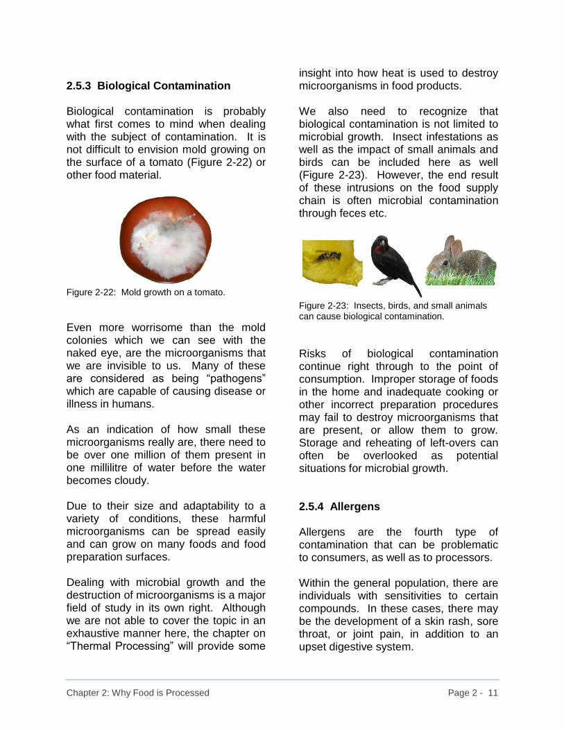
2.5.3 Biological Contamination Biological contamination is probably what first comes to mind when dealing with the subject of contamination. It is not difficult to envision mold growing on the surface of a tomato (Figure 2-22) or other food material.
Figure 2-22: Mold growth on a tomato.
Even more worrisome than the mold colonies which we can see with the naked eye, are the microorganisms that we are invisible to us. Many of these are considered as being “pathogens” which are capable of causing disease or illness in humans. As an indication of how small these microorganisms really are, there need to be over one million of them present in one millilitre of water before the water becomes cloudy. Due to their size and adaptability to a variety of conditions, these harmful microorganisms can be spread easily and can grow on many foods and food preparation surfaces. Dealing with microbial growth and the destruction of microorganisms is a major field of study in its own right. Although we are not able to cover the topic in an exhaustive manner here, the chapter on “Thermal Processing” will provide some
insight into how heat is used to destroy microorganisms in food products. We also need to recognize that biological contamination is not limited to microbial growth. Insect infestations as well as the impact of small animals and birds can be included here as well (Figure 2-23). However, the end result of these intrusions on the food supply chain is often microbial contamination through feces etc.
Figure 2-23: Insects, birds, and small animals can cause biological contamination.
Risks of biological contamination continue right through to the point of consumption. Improper storage of foods in the home and inadequate cooking or other incorrect preparation procedures may fail to destroy microorganisms that are present, or allow them to grow. Storage and reheating of left-overs can often be overlooked as potential situations for microbial growth. 2.5.4 Allergens Allergens are the fourth type of contamination that can be problematic to consumers, as well as to processors. Within the general population, there are individuals with sensitivities to certain compounds. In these cases, there may be the development of a skin rash, sore throat, or joint pain, in addition to an upset digestive system.
Chapter 2: Why Food is Processed Page 2 - 12
Individuals with food allergies tend to experience much more violent or severe reactions to certain foods than those with food sensitivities. Allergies trigger responses from the body’s immune system which can include anaphylaxis or “anaphylactic shock”. In these cases, there can be a tightening or constriction of the breathing passages, a sudden drop in blood pressure, dizziness, or loss of consciousness. Food materials or ingredients that are considered to be allergens include (based on Health Canada website information (2)):
• Eggs
• Milk
• Mustard
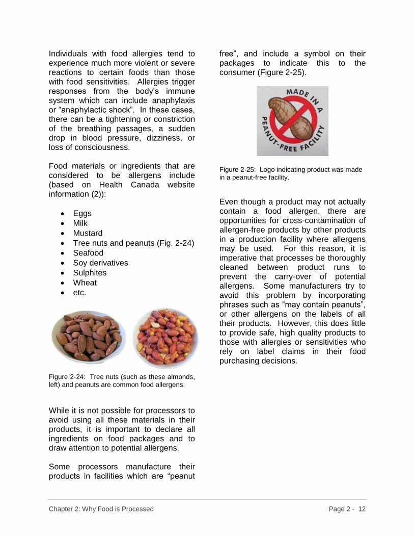
• Tree nuts and peanuts (Fig. 2-24)
• Seafood
• Soy derivatives
• Sulphites
• Wheat
• etc.
Figure 2-24: Tree nuts (such as these almonds, left) and peanuts are common food allergens.
While it is not possible for processors to avoid using all these materials in their products, it is important to declare all ingredients on food packages and to draw attention to potential allergens. Some processors manufacture their products in facilities which are “peanut
free”, and include a symbol on their packages to indicate this to the consumer (Figure 2-25).
Figure 2-25: Logo indicating product was made in a peanut-free facility.
Even though a product may not actually contain a food allergen, there are opportunities for cross-contamination of allergen-free products by other products in a production facility where allergens may be used. For this reason, it is imperative that processes be thoroughly cleaned between product runs to prevent the carry-over of potential allergens. Some manufacturers try to avoid this problem by incorporating phrases such as “may contain peanuts”, or other allergens on the labels of all their products. However, this does little to provide safe, high quality products to those with allergies or sensitivities who rely on label claims in their food purchasing decisions.

Chapter 2: Why Food is Processed Page 2 - 13
2.6 Summary Comments It is a common misconception that maintenance or enhancement of food quality is limited to within the confines of the food processing plant. In actual fact, quality is influenced by numerous factors along the entire food chain from a time even before the seeds of a crop are planted until the time the food is consumed. More and more food processors are becoming mindful of the impact of raw material production and handling on their ability to manufacture high quality finished products. They are becoming acutely aware of the effects of distribution, handling, storage, and end-product preparation on the safety and quality of the products that the consumer eats. For this reason, there is an increasing tendency among food producers to adopt the approach of managing the entire food production and distribution chain. Throughout the previous discussion, the importance of food processing has been repeatedly demonstrated. In conjunction with this, there is the need to be constantly aware of the fact that an underlying requirement of food processing is to maintain a safe and high quality food supply. Failure to acknowledge this fact can doom a processor to failure.
2.7 References 1. “Wasted: How America is Losing Up
to 40% of Its Food from Farm to Fork to Landfill”. Dana Gunders. Natural Resources Defense Council (NRDC) Issue Paper IP:12-06-B, August 2012. Available on-line at: www.nrdc.org/sites/default/files/wasted-food-IP.pdf (accessed March 2018).
2. “Common Food Allergens”. Health Canada Website. Available on-line at: www.canada.ca/en/health-canada/services/healthy-living/your-health/food-nutrition/food-allergies.html (accessed March 2018).

Chapter 3: Historical Development of Food Processing Page 3 - 1
3. Historical Development of Food Processing 3.1 Introduction Exactly where and when food processing actually began is open to speculation. However, even during the hunting and gathering stages of human development, there may have been some forms of basic food processing. Drying of meats and berries (Figure 3-1) in the open sun or over a fire created new forms of food that could be more easily transported, and were not subjected to the ravages of spoilage that would affect the unprocessed form of the same food.
Figure 3-1: Dried blueberries have enhanced shelf-life over their fresh counterpart.
Naturally occurring fermentations that changed milk to cheese or yogurt (Figure 3-2), and changed barley mash or grape juice to rather pleasantly intoxicating beverages were known to exist in prehistoric times.
Figure 3-2: Milk can be converted to cheese and yoghurt by means of fermentations.
3.2 Early Advances in Food Processing As fascinating as these prehistoric developments are, it was not until the “Middle Ages” that any science-based food processing activities actually took place. Prior to this, food processing may have been considered to be an art passed down through successive generations as a method of survival through securing an adequate food supply in time of need. Much of what follows is a summary of information presented by C.W. Hall and G.M. Trout in their book published in 1968 on “Milk Pasteurization”. Initial discussion of the historical development of food processing will focus on the application of heat to delay the onset of food spoilage. As previously noted, this preservation technique goes back to pre-recorded history. However, the application of heat to liquid products is a more recent development which is believed to have started in the late 18th Century. In 1765, a noted Italian Catholic priest named Spallanzini demonstrated that meat extracts could be preserved in sealed glass flasks by

Chapter 3: Historical Development of Food Processing Page 3 - 2
boiling them in water for about one hour (Hall and Trout, 1968). In 1782, the Swedish scientist Sheele used heat in the preservation of vinegar. It was not until 1804 that food preservation by thermal processing methods took a major step forward. At this time, France was at war and Napoleon’s supply lines were stressed to the point that his armies were doing poorly on inadequate rations that were often spoiled, unwholesome, or generally unpalatable. Similarly, sailors in the navy and on merchant ships were suffering the ill effects of poor diets, including scurvy. In 1811, Nicolas Appert published a treatise on “The Art of Preserving All Kinds of Animal and Vegetable Substances for Several Years” (Britannica on-line). Appert found that if foods were sealed inside containers and heated sufficiently, the product would not spoil, as long as the container remained closed. Appert’s processing technology won him 12,000 francs as a prize for developing a method of preserving food and began the age of food canning as we now know it. In 1824, William Dewees, a professor of obstetrics at the University of Pennsylvania, recommended that milk should be heated to near boiling and cooled prior to using the milk to feed babies (Hall and Trout, 1968). He had observed that the tendency of milk to decompose in hot weather was diminished by boiling the milk. While it would still be another 40 years before this procedure was understood, its effects on infant health were certainly dramatic.
Around 1790, Europe, and in particular England, entered into a period that is commonly referred to as the “Industrial Revolution”. Technological advances were taking place at a rapid rate and lifestyles were beginning to change. As industrialization spread, people from rural areas began to move to the cities, and large urban areas developed. In the Midlands of England, the burgeoning textile industry contributed greatly to the expansion of cities and towns. Increased distances between people in the cities and rural sources of food added to the problems of providing adequate and nutritious food to the masses (Figure 3-3). No longer could people go to small local markets or harvest their own fresh produce. The time taken to get foods to markets in the larger centres was also a significant obstacle to be overcome. Within a short time, the “Industrial Revolution” spread to the emerging economy of the United States.
Figure 3-3: Urbanization introduced time and distance factors to the food supply chain.
3.3 Advances by Louis Pasteur In the mid-1800’s, France was going through what many considered to be a national disaster. A mysterious situation had arisen in the form of wine spoilage which was plaguing the country. During the period from 1860 to 1864, the

Chapter 3: Historical Development of Food Processing Page 3 - 3
famous French scientist Louis Pasteur was summons by the Emperor to work on solving this problem. He found that if the wine was heated to a sufficiently high temperature, and if it was held there for a suitable length of time, the contaminating microorganisms would be inactivated while the characteristics of the wine would still be retained. He used temperatures in the range of 50° to 60°C. Pasteur later applied his process of “par-boiling” or “under-boiling” to the treatment of beer (at temperatures of 50° to 55°C). In spite of the fact that Pasteur’s process of “pasteurization” is so widely applied to milk (Figure 3-4), there do not seem to be any references in Pasteur’s records that he ever applied his principles to milk himself (Hall and Trout, 1968).
Figure 3-4: Pasteur did not heat-treat milk even though the process bears his name.
3.4 Modern Advances in Food Processing In 1881, the first commercial milk pasteurizer was introduced in Germany. 1889 saw the establishing of the world’s first dispensary for the provision of heat-treated milk for infants. This operation was set up in New York City by Dr. Henry Koplik, a pediatrician. At the start of the 20th Century, many people felt that pasteurization of milk was undesirable and unnecessary. It was the growth of cities that changed all this by increasing the distance milk had to be transported and the time it took to reach the consumer. Heat treatment reduced this spoilage problem. In 1908, Chicago became the first city in the world to require the pasteurization of the city’s milk supply (Hall and Trout, 1968). In 1909, the city passed the first compulsory pasteurization law in the United States. It is interesting to note that the people of this time felt the same level of anxiety and heightened emotionalism with pasteurization as many people felt during the late 20th Century with the advent of food irradiation. There have been many significant developments in technology and processing equipment design over the years that have enhanced the reliability and economics of the pasteurization process, as well as improving product quality. These include advances in thermal processing equipment (Figure 3-5) and heat recovery as well as corresponding developments in packaging and distribution that have contributed to the quality and shelf-life of dairy-based products over these years.

Chapter 3: Historical Development of Food Processing Page 3 - 4
Figure 3-5: Plate heat exchangers have improved thermal processing of liquid products.
Aseptic packaging was a significant food processing development during the 20th Century. In this process developed by Tetra Pak of Lund, Sweden, commercially sterile liquid products are brought together with sterile packaging in a sterile area of a packaging machine. Packages are filled and sealed prior to leaving the sterile zone for warehousing, distribution, and sale to consumers (Tetra Pak International, 2015). Once packaged, the product has a shelf-life of nine months or more under ambient storage conditions as found in most homes. The individual serving sizes of these packages are often referred to as “drink boxes” (Figure 3-6). Aseptic packaging provides enhanced shelf-life of liquid food products. Examples include milk and fruit juices, as well as a host of other products such as soups and sauces containing particulates. There are now other companies that have perfected their own formats of aseptic packaging to expand the range of available aseptic products.
Figure 3-6: Aseptically packaging of beverages in “drink boxes” was a major processing advance in the 20th century.
While perhaps not being as exciting as the development of canning or aseptic packaging, many other advances have been made in food processing as well. Everyday, travellers see examples of this as they view refrigerated trucks and transport trailers (Figure 3-7) carrying perishable materials along major highways.
Figure 3-7: Refrigerated trucks have done much to improve distribution of perishable products.
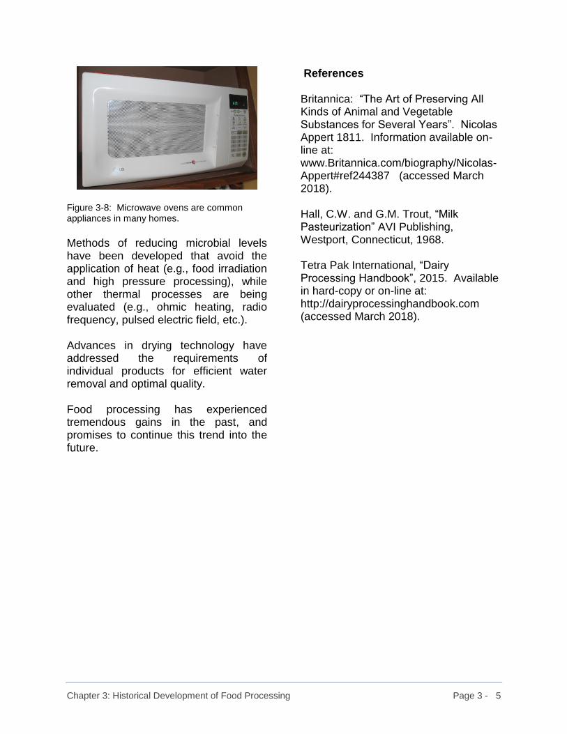
Microwave ovens (Figure 3-8) have become acceptable appliances in almost every home in North America, opening up previously unavailable opportunities for food processors who are competing for a share of this lucrative “convenience food” market.
Chapter 3: Historical Development of Food Processing Page 3 - 5
Figure 3-8: Microwave ovens are common appliances in many homes.
Methods of reducing microbial levels have been developed that avoid the application of heat (e.g., food irradiation and high pressure processing), while other thermal processes are being evaluated (e.g., ohmic heating, radio frequency, pulsed electric field, etc.). Advances in drying technology have addressed the requirements of individual products for efficient water removal and optimal quality. Food processing has experienced tremendous gains in the past, and promises to continue this trend into the future.
References Britannica: “The Art of Preserving All Kinds of Animal and Vegetable Substances for Several Years”. Nicolas Appert 1811. Information available on-line at: www.Britannica.com/biography/Nicolas-Appert#ref244387 (accessed March 2018). Hall, C.W. and G.M. Trout, “Milk Pasteurization” AVI Publishing, Westport, Connecticut, 1968.
Tetra Pak International, “Dairy Processing Handbook”, 2015. Available in hard-copy or on-line at: http://dairyprocessinghandbook.com (accessed March 2018).

Chapter 4: Background Skills for Food Processing Page 4 - 1
4. Background Skills for Food Processing
4.1 Introduction Before beginning the actual study of “Food Processing Concepts”, it is important to establish some background skills that are essential for working in this field. Being able to organize information in a clear, logical, and disciplined manner is critical in characterizing any food manufacturing process. The separation of important information or facts from non-essential material is one of the first steps on the way to understanding a process. Based on the organization of available relevant information, it is generally possible to evaluate how well a process is functioning and often identify where improvements can be made. By reducing losses, improved yields or efficiencies can be realized, thereby saving time, materials, and money. It is also important to have a good grasp of the fundamentals of temperature and pressure as well as understanding density, specific gravity, mass balances, and related calculations. In this section, each of these topics is discussed briefly in preparation for further work.
4.2 Organizing Information One of the best ways to organize information about a particular process is to draw a sketch of it. No high level of artistic talent is required; a simple series of “boxes” joined by arrows is all that is really needed. Each box can be labelled as being an individual step in the process, or it can represent a specific piece of equipment. Individual steps can be referred to as a “unit operation”. By arranging these “boxes” in the proper sequence, a “process flow diagram” can be prepared to summarize the key steps in the process. Additional information regarding temperatures, moistures, and flowrates, etc., can be added to make the process flow diagram (or PFD) as comprehensive as desired. Generally, care is taken not to make the diagram too overwhelming or too confusing. Many people like the names of unit operations to end in the letters “er” or “or”, such as dryer, cooker, cooler, or collector. Other people prefer to have the names of the processing steps end in the letters “ing” such as drying, cooking, cooling, or collecting. These are not hard and fast rules, but only guidelines. There are certainly exceptions that can be easily accommodated. Frequently, one person’s idea of what a flow diagram looks like for a particular process will differ from another person’s idea of a diagram for the same process. This is based on what each individual considers to be a unit operation and how they have broken the process down into its component steps. While a certain degree of difference should be expected, care must be taken not to overlook any key processing steps.

Chapter 4: Background Skills for Food Processing Page 4 - 2
For illustrative purposes, a food-related process that might be performed in a household kitchen can be considered. In this example, a batch of chocolate brownies is being prepared, with the finished product being into cut squares and placed on a plate ready for serving. Before proceeding any further, it is necessary to understand the procedures involved in making the chocolate brownies, which is best done by simply listing all of the steps that are involved. In assembling this list, no steps should be omitted - no matter how simple they seem to be. Steps Involved in Preparing Chocolate Brownies 1. Assemble ingredients. 2. Assemble necessary utensils and
equipment. 3. Melt ingredients as necessary
(e.g., chocolate) 4. Add ingredients in proper order. 5. Mix ingredients in bowl. 6. Pour batter into pan. 7. Bake for desired length of time at
specified temperature. 8. Remove baked brownies from
oven. 9. Allow brownies to cool. 10. Prepare icing while brownies are
cooling (if you like really sweet brownies).
11. Add icing to brownies. 12. Let icing set. 13. Cut brownies into squares. 14. Place squares on plate. 15. Serve brownies to guests.
Quantities required in the recipe are not specified in this list; and with the exception of melting the chocolate, no ingredients are even mentioned.
Figure 4-1 shows the finished product before and after cutting into individual servings.
Figure 4-1: Chocolate Brownies: Before and after cutting of individual servings.
Now that the basic steps have been laid out, an attempt can be made to develop a process flow diagram listing the unit operations, as shown in Figure 4-2. Beginning with the “box” in the top left corner of the diagram, the ingredients are being taken out of their respective storage areas and prepared for work by assembling or staging them. The “ingredient storage” may not be an integral part of the process for preparing the chocolate brownies, but it does provide a convenient starting point from which to proceed with the subsequent processing steps. The assembling of the various utensils to perform the mixing of ingredients and addition of icing etc., would be entirely optional in the process flow diagram. The decision of what additional information should be included in the process flow diagram is up to the individual drawing it. However, inclusion of too much extra information may produce a cluttered diagram that is confusing and difficult to follow. In Figure 4-2, chocolate has been taken aside and melted prior to being mixed with the other ingredients in the second

Chapter 4: Background Skills for Food Processing Page 4 - 3
box from the top in the middle column. Icing has also been prepared separately from the main mixing process and has been added at the appropriate time. Care should be taken in following the lines from the “Ingredient Staging” to the “Preparation of Icing” and to the
“Chocolate Melting” since they do not follow a straight pathway. In some PFD’s, it may be necessary to have lines such as these bend and cross other lines to reach their appropriate destinations.
Figure 4-2: Process flow diagram for preparing chocolate brownies. (Steps may be numbered for ease of reference)

Chapter 4: Background Skills for Food Processing Page 4 - 4
An example of how additional information may be added is shown by the arrows indicating that heat is added in the “Baking” step and removed in the “Cooling” step. If a more thorough treatment of the brownie process is desired, temperatures and times could be added to the baking process. Basically, the process flow diagram can be considered as an aid to understanding the overall process and its material flows without getting into the exact details of how the product is being made or prepared. Having done this for a rather basic kitchen process, a similar exercise could be conducted for an industrial process. Figure 4-3 shows a process flow diagram or “PFD” for making apple juice. It is based on a process outlined by “The Bioindustrial Group” of Novo Industri A/S in Bagsvaerd, Denmark (Novo Industri A/S). In this process whole apples or the cores and peels of apples from other operations (such as the making of apple sauce or pie filling) are brought together and literally mashed into a pulp by a hammer mill. Large hammer heads continuously strike the apple pieces as they pass through the mill. Once the mash reaches the desired consistency, pectinase enzymes are added to break down the structure of the pectin that holds the flesh of the fruit together. It takes about an hour for this part of the process to occur, so the apple mash is held in an unstirred “holding tank” at 30°C for this amount of time. By breaking down the pectins, the fleshy portions of the apples lose their ability to hold the juice that the processor wants to extract. After the enzyme has had a chance to break
down the pectin, the mash is pressed or squeezed to remove as much liquid as possible. The solids, or “pomace” as it is called, leave the process for disposal or alternate use. The remaining liquid is passed through a mesh screen to remove any additional pieces of apple, which then join the pomace from the previous step. A second pectinase enzyme, which operates under somewhat different conditions from the first enzyme, is then added to remove the last bits of apple solids that may be clouding the solution. The mixture is held at a relatively high temperature of 54°C for up to two hours to allow the enzyme to break down the remaining pectin. Once this has taken place, the mixture is filtered and the resultant juice can go on for further processing. As can be seen in Figure 4-3, the process flow diagram for the industrial juice process is quite similar to the one constructed for making brownies. One slight difference, however, is that pieces of equipment are named in the apple juice process, whereas descriptions of the steps are used for the making of the brownies. Either way may be acceptable, depending on the end use of the diagram and the preferences of the individuals requiring the diagram.

Chapter 4: Background Skills for Food Processing Page 4 - 5
Figure 4-3: Process flow diagram for apple juice production (based on Bioindustrial Group, Novo Industri A/S).
Chapter 4: Background Skills for Food Processing Page 4 - 6
4.3 Dimensional Analysis For those just beginning to study food processing, one of the more troublesome aspects may be how to approach problem solving and deal with the information that is provided. The previous section showed how drawing a process flow diagram can help in understanding particular manufacturing sequences. In a similar manner, drawing a quick diagram can be of assistance in organizing the information in a problem that must be solved. Once the information is organized, decisions can be made regarding how to deal with it. This is where the concept of “dimensional analysis” becomes useful. In dimensional analysis, not only is the size, or magnitude, of the numbers used in the calculations, but their units are also employed. In this way, the confusion about whether to divide by a number or multiple by it can be substantially reduced. This can be readily shown through a sample calculation. Sample Calculation 4-1 Many processing calculations involve conversions of time (Figure 4-4) from one set of units to the next. Often this will involve finding the number of packages produced in a day when you know the production speed in packages per minute. Here, we will calculate the number of seconds in a day.
Figure 4-4: Time conversions are very common in processing calculations.
Solution: Most people know that there are 60 seconds in a minute, 60 minutes in an hour, and 24 hours in a day. This knowledge is all that is needed to solve the problem. Seconds per day = 60 seconds x 60 minutes x 24 hours minute hour day minute hour day = 86,400 seconds / day Notice that the “minutes” below the line in the first term of the equation will cancel out the “minutes” above the line in the second term; and the “hours” below the line in the second term will cancel out the “hours” above the line in the third term. The units remaining are “seconds / day”, which is what was requested to be determined in the initial question. This solution can be streamlined somewhat by drawing a single horizontal line on which to build a sequence of calculations. Quantities above the line will be multiplied by each other, as will quantities below the line. However, quantities below the line will be divided into quantities above the line.
Chapter 4: Background Skills for Food Processing Page 4 - 7
Repeating the example above, it follows that: Seconds per day = 60 seconds | 60 minutes | 24 hours minute | hour | day = 86,400 seconds / day As can be seen by the way this calculation is laid out, division and multiplication are still conducted in the same manner as in the first method, but the multiplication symbols (i.e., the “x’s”) have been replaced with vertical lines, and the individual dividing lines are replaced by one single horizontal line.
Sample Calculation 4-2 Calculate the number of grams in an ounce. Solution: In order to do this calculation, some basic conversion factors are needed. There are 16 ounces in a pound and 2.204 pounds in a kilogram. 1 kilogram is made up of 1,000 grams. Ounces can be abbreviated to “oz” and pounds can be abbreviated to “lb”. Grams per ounce = 1,000 g | kg | lb . kg | 2.204 lb | 16 oz = 28.36 g / oz As can be seen, the units of kg and lb cancel out and leave “grams per ounce” as the final set of units. Since the numerical value is 28.36, there are 28.36 grams in one ounce.
The beauty of dimensional analysis is that it helps detect errors in a calculation. In general, if the units do not make sense, the calculation is incorrect. Sample Calculation 4-3 The determination of grams per ounce from the previous sample calculation will now be repeated with a deliberate error to show how dimensional analysis can be used as an error-indicating tool. Solution (with error): Grams per ounce = 1,000 g | 2.204 lb | lb . kg | kg | 16 oz
= 137.75 g lb2 / kg2 oz (This is incorrect !!!) While the size of the actual number may not provide a clue as to whether or not the calculation is correct, alarms should immediately go off at the sight of the units obtained in this calculation. The desired units were “grams per ounce”. Instead, units of “grams pounds-squared per kilogram-squared ounce” were obtained. The only way these strange units could have resulted would have been through an error in setting up the equation. Upon inspection, it can be seen that the “2.204 lb per kg” factor is upside down in the equation. This means that instead of multiplying by “2.204 lb per kg”, it should have been divided into the 1,000 g / kg value. It is strongly recommended that units or dimensions be included as part of all calculations. In cases where the

Chapter 4: Background Skills for Food Processing Page 4 - 8
calculations are more complex, the advantages of dimensional analysis are even more pronounced. 4.3.1 Practice Problems – Dimensional Analysis Dimensional analysis is particularly useful in doing conversions from one set of measurements to another. Many nations of the world have formally adopted the International System of Units (SI) which is based on the metric system. However, many individuals and food processors still work in non-SI units such as inches, feet, miles, ounces, pounds, and quarts. In addition, the United States still retains the “British System” of measurement. For these reasons, it is important to be able to do the necessary conversions. Given that there are: 2.54 cm per inch 12 inches per foot 5,280 feet per mile 100 cm per metre 1,000 cm3 per litre π = 3.14159 Answer the following questions. These examples are intended to illustrate the use of dimensional analysis and are not meant to be difficult. 1. A piece of processing equipment
is 5 foot 6 inches long by 4 foot 3 inches wide and 10 feet high, calculate the dimensions in centimetres and metres. Draw a diagram first (Figure 4-5) and express your final answers to two decimal places.
Figure 4-5: Diagram for box calculation.
(Answer: 167.64 cm long by 129.54 cm wide by 304.80 cm high, or 1.67 m long by 1.30 m wide by 3.05 m high)
2. Calculate the volume of a cylindrical tank that is 3 feet high by 1.75 feet in diameter (Figure 4-6). Express your answer in litres to one decimal place. The volume of a cylinder is: π r2 h or π d2 h / 4.
Figure 4-6: Diagram of cylinder.
(Answer: 204.3 litres)
Hint: Convert the dimensions to centimetres before calculating the volume of the tank.
3. Calculate the number of metres
and kilometres in a mile (to one decimal place). (Answer: 1,609.3 metres and 1.6 kilometres)

Chapter 4: Background Skills for Food Processing Page 4 - 9
4.4 Temperature Temperature measurements are used in our daily lives as a matter of routine without much regard for how they came into being, or their significance in food processing. While outside temperatures affect personal activities and how people dress etc., processing temperatures affect reaction rates as well as product performance and storage life. There are four basic temperature scales in existence today: Fahrenheit, Celsius, Kelvin, and Rankine. The Rankine scale is seldom used. In order to understand the conversion from one temperature scale to another, a short digression on the historical development of these scales is warranted. There are numerous versions of how events transpired, so you may have heard different stories of this topic. The important thing is to recognize the efforts that went on during the late 1600’s and early to mid-1700’s to find a method to quantify and reliably measure temperatures. In 1724, the German-Dutch physicist Gabriel Daniel Fahrenheit (1686 to 1736) invented the mercury thermometer and developed the temperature scale which bears his name (CAPGO on-line). He and others had seen the need to quantify the heat content of materials. Fahrenheit used the height of a vertical column of mercury in a sealed glass tube as his measuring devise. When heated, the mercury expanded and the column height rose in the glass tube. When cooled, the mercury contracted and its column height dropped in the sealed glass tube. Several stories exist that
explain how Fahrenheit set up the reference points on his temperature scale. Regardless of which story you believe, the basis for his work was somewhat confusing to say the least. Simplifying one of the stories greatly, it seems that Fahrenheit selected a lower reference temperature for his scale based on the lowest temperature he could achieve in a saturated solution of salt and water mixed with ice. He called this point 0°F. According to some beliefs, the upper reference point of 100°F was established as being normal body temperature. However, due to the fact that Fahrenheit was running a bit of a fever that day, his temperature was somewhat elevated and when the fever went down, his body temperature was actually 98.6°F. He then divided the interval between his two reference temperatures into 100 equal divisions or “degrees”. By extrapolating his scale, Fahrenheit found that water boiled at 212°F at mean sea level. Pure water froze at 32°F on his scale. As can be seen, Fahrenheit’s temperature scale was founded on a certain lack of structure and discipline. A few years later, in 1742, Anders Celsius, a Swedish scientist, developed his own temperature scale (CAPGO on-line). Celsius used the boiling point of water and its freezing point as his two basic references. He divided this temperature range into one hundred equal “degrees”. It is interesting to note that the original scale was exactly the reverse of what we use today. Initially, Celsius had water freezing at 100 degrees and boiling at 0 degrees. This scale was reversed after his death.

Chapter 4: Background Skills for Food Processing Page 4 - 10
With advances in the understanding of how gases behaved under various conditions of temperature and pressure, the concept of a point called “absolute zero” was developed. If the temperature of an “ideal” gas is lowered, its volume decreases. It was postulated that there would ultimately be a temperature where all molecular motion would cease. This temperature would be “absolute zero”. Although “absolute zero” has never actually been achieved, scientists have come extremely close to it in the laboratory. Being aware of “absolute zero”, the British mathematician and physicist William Thomson Kelvin proposed the Kelvin temperature scale in 1848. He reasoned that there were no temperatures below “absolute zero”, so he would take this point as the “zero” on his temperature scale. He extrapolated the Celsius scale down to “absolute zero” and found it to be 273.15 Celsius degrees below the freezing point of water. On Kelvin’s scale, the freezing point of water is 273.15K (equivalent to 0°C) and the boiling point of water is 373.15K (equivalent to 100°C). The Kelvin scale does not use the degree symbol nor the word “degrees” in expressing it. The final temperature scale which may be encountered, although quite rarely, is the Rankine scale. It is essentially the equivalent of the Kelvin scale, but is based on the Fahrenheit scale rather than on the Celsius scale. William John Macquorn Rankine was a Scottish engineer who put forward his new temperature scale in 1859. It too was based on using “absolute zero” as its starting point just like Lord Kelvin’s temperature scale. Rankine
extrapolated Fahrenheit’s temperature scale back to “absolute zero”, which he found was 459.67 degrees below Fahrenheit’s zero reference point. This meant that water froze at 491.67°R (i.e., 32°F) and water boiled at 671.67°R (i.e., 212°F). Rankine temperatures may be seen written with or without the degree symbol (i.e., °R or simply R). Knowing the relationships between the boiling and freezing points of water on the Fahrenheit and Celsius temperature scales allows for the conversion of one temperature reading to another. Figure 4-7 shows how this can be done.
Figure 4-7: Comparison of Fahrenheit and Celsius Temperature Scales.
In Figure 4-7, both the Fahrenheit and Celsius temperatures are shown on opposite sides of a “thermometer” scale. The freezing point of water is 32°F or 0°C and the boiling point of water at mean sea level is 212°F or 100°C. This indicates that the temperature difference of 180 Fahrenheit degrees is equal to a temperature difference of 100 Celsius

Chapter 4: Background Skills for Food Processing Page 4 - 11
degrees. Therefore, a change in temperature of one Celsius degree (i.e., 1.0 C°) is equivalent to a temperature change of 1.8 Fahrenheit degrees (i.e., 1.8 F°). It should be noted that when discussing temperature differences, reference is made to them as “Fahrenheit degrees” or “Celsius degrees”. When speaking of actual temperatures, one would say “degrees Fahrenheit” or “degrees Celsius”. The basis for temperature conversions has now been established. To convert from a given Fahrenheit temperature to its equivalent Celsius temperatures, take the Fahrenheit temperature, subtract 32 Fahrenheit degrees and divide the resultant value by 1.8 (see equation 4-1). Degrees Celsius =
°C = (Fahrenheit temp - 32 F°) / 1.8 (Eq’n 4-1)
In order to convert from a Celsius temperature to its equivalent Fahrenheit temperature, multiply the Celsius temperature by 1.8 and add 32 Fahrenheit degrees as shown in equation 4-2. Degrees Fahrenheit =
°F = (Celsius temp x 1.8) + 32 F° (Eq’n 4-2)
In any scientific field of study, there are frequent references to the Kelvin temperature scale, so a knowledge of the conversion from Celsius temperatures to their Kelvin equivalents is important. Pure water freezes at 0°C and at 273.15 K, and a temperature difference of one degree on the Celsius scale is identical to a temperature difference of one degree on the Kelvin
scale. Therefore, to convert from Celsius to Kelvin, all that has to be done is to add 273.15 to the Celsius temperature as shown in equation 4-3. Kelvin temperature = K = Celsius temperature + 273.15
(Eq’n 4-3) The reverse calculation is indicated in equation 4-4: Celsius temperature = °C = Kelvin temperature - 273.15
(Eq’n 4-4) As stated above, a temperature difference of one degree on the Celsius scale is identical to a temperature difference of one “degree” on the Kelvin scale. This fact will become very important in dealing with the heating and cooling of materials when temperature changes are calculated. If a temperature change is required in Kelvin units, it will be the same as the temperature change in Celsius degrees. This means that it is not necessary to convert Celsius temperatures to Kelvin before calculating the temperature difference in Kelvin units. For example, when heating a material from 30°C to 55°C, the temperature change will be 25 C° which is identical to 25 Kelvin “degrees”. To prove this, 30°C is equal to 303.15 K and 50°C is equal to 328.15 K. The difference between 303.15K and 328.15K is 25 Kelvin “degrees”. Therefore, it is not necessary to convert the Celsius temperatures to Kelvin when a temperature difference is required in Kelvin “degrees”. There is one additional concept that should be mentioned in discussing

Chapter 4: Background Skills for Food Processing Page 4 - 12
temperature readings, and that concerns “mean sea level”. The boiling point of water is highly dependent upon atmospheric pressure. As you move to higher elevations, atmospheric pressure decreases and the boiling point of water goes down. As a result, water may not boil at 100°C in all locations - this is especially true in the case of a city such as Denver, Colorado which is known as “The Mile High City”. In order to standardize the boiling point of water, a benchmark reference elevation was established. This reference elevation was sea level with “normal atmospheric pressure”. Since sea level varies with the changes in the tides, an average or “mean” sea level was used for this purpose. Sample Calculation 4-4 Convert 190°F to its Celsius equivalent Solution: Using equation 4-1: °C = (Fahrenheit temp - 32 F°) / 1.8 = (190 -32) / 1.8 °C = 158 / 1.8 °C = 87.8°C Therefore, 190°F is equivalent to 87.8°C or approximately 88°C.
Sample Calculation 4-5 Convert 60°C to its Fahrenheit equivalent. Solution: Using equation 4-2: °F = (Celsius temp x 1.8) + 32 F° = (60 x 1.8)°F + 32 F° = 108°F + 32F° = 140°F Therefore, 60°C is equivalent to 140°F. Sample Calculation 4-6 Convert 100°C (boiling point of water) to Kelvin Solution: Using equation 4-3: K = Celsius temperature + 273.15 = 100°C + 273.15 = 373.15 K Therefore, the boiling point of water at mean sea level is 373.15 K (note that there is no degree symbol associated with Kelvin temperatures)
Chapter 4: Background Skills for Food Processing Page 4 - 13
Sample Calculation 4-7 Convert -20°F to its equivalent Celsius temperature. Solution: Using equation 4-1: °C = (Fahrenheit temp - 32 F°) / 1.8 = (-20 - 32) / 1.8 °C = -52 /1.8 °C = -28.9°C Therefore, -20°F is equal to -28.9°C or approximately -29°C.
4.4.1 Practice Problems – Temperature 1. Convert normal body temperature
of 98.6°F to its Celsius equivalent. (Answer: 37.0 °C)
2. Typically, autoclaves and
sterilizers run under pressure with temperatures of approximately 121°C. Convert this temperature to its Fahrenheit equivalent. (Answer: 249.8°F or approximately 250°F)
3. What is the Fahrenheit equivalent
of -40 C ? (Answer: - 40°C = - 40°F; This is the only temperature at which the two are equal)
4. Convert 293 K to its Fahrenheit
equivalent. (Answer: 293 K equals 19.85°C which in turn equals 67.7°F, or approximately 68°F)

Chapter 4: Background Skills for Food Processing Page 4 - 14
4.5 Pressure Pressure is a measurement which many people find confusing. This is due in part to the number of units in which pressure is expressed. In SI units, pressure is quoted in units of “kiloPascals”. However, in some instances, other units employed. When car tires are inflated, the recommended pressures are most often expressed in “pounds per square inch”. Older style barometers that people have in their homes give the atmospheric pressure in “inches of mercury” and many medical instruments report pressures in “millimetres of mercury”. Just to add to the confusion, pressures are also expressed in “atmospheres”, “feet of water”, and “bars”. On top of the potential confusion arising from the variety of units, there is also the added factor of “absolute” and “gauge” pressures. Perhaps the best way to begin understanding pressure measurements is to start with one basic unit and expand from there. “Pounds per square inch” will be used as a starting point and as a basis for discussion of the concept of atmospheric pressure. In the previous section, it was stated that the boiling point of water was affected by atmospheric pressure and that the reference point for this measurement was at “normal atmospheric pressure” at “mean sea level”. Assume that a point is established on an ocean beach at the half-way point between high and low tides. At this point, there is a column of air which extends upwards to the limits of the earth’s atmosphere (i.e., up into
the stratosphere). On a clear day with fair weather, a column of air one inch square and the height of the atmosphere weighs 14.7 pounds. This means that the downward pressure exerted by this column of air is equal to 14.7 pounds per square inch (Figure 4-8). This is now the starting point for all of the other pressure measurements.
Figure 4-8: Force of a column of air on a one square inch surface is 14.7 pounds.
Since 14.7 pounds per square inch represents normal atmospheric pressure, it is often referred to as “one atmosphere” for simplicity. Allowing for the fact that 14.7 pounds per square inch, or 14.7 psi, is a numerical value having the associated units of pounds and square inches, it can be converted to its equivalent of 101.325 kiloPascals, or 101.325 kPa. In some cases, the 101.325 kPa value was

Chapter 4: Background Skills for Food Processing Page 4 - 15
considered somewhat awkward to deal with, so a new unit called a “bar” was coined to represent a pressure of 100.0 kPa. A “bar” is slightly less than one atmosphere. In order to measure atmospheric pressure, devices known as barometers were developed. They typically consisted of a glass tube about one metre long with one end sealed. The tube was then filled with mercury and inverted with the open end submerged in an open mercury reservoir. The theory here is that the force of the atmospheric pressure pushing down on the mercury reservoir will support the column of mercury in the closed tube. The upper sealed end of the tube is under vacuum and an equilibrium is established between the pressure of the column of mercury and atmospheric pressure. The height of this mercury column at normal atmospheric pressure was found to be 29.92 inches or 760 mm. These two values then became the basis for pressure measurements in terms of “inches of mercury” and its metric equivalent of “mm of mercury”, or “inches Hg” and “mm Hg”. In dealing with fluids, water is the most common fluid that is pumped through pipes. Based on a comparison of the densities of water (1.0 grams per millilitre) and mercury (13.6 grams per millilitre), the height of a column of water equivalent to the 29.92 inch column height of mercury was found to be about 33.8 feet. This is a useful factor in determining how much pressure is necessary when pumping water upwards. It is also useful in determining the pressure forces on the surfaces of submerged objects such as submarines and human divers. For every 33.8 feet
below the surface of fresh water an object goes, the pressure on its surface increases by one atmosphere or 14.7 psi. Having dispensed with the origins of many of the pressure units in use today, it now remains to explain “gauge pressures” and “absolute pressures”. Consider once again the column of atmospheric air that is constantly pushing down on all surfaces. Even though it is not noticeable, there is a force of 14.7 pounds acting on every square inch of surface area, including our bodies, or every square inch of the table at which you may be sitting. If you were to take your thumb and apply an additional force of 5 pounds per square inch on the surface of a table, the total pressure on that small area would be 19.7 psi (i.e., 14.7 psi plus the additional 5 psi from your thumb). This is the absolute pressure acting on that portion of the book. Since the 14.7 psi pressure of the atmosphere is relatively constant on all surfaces, it is an attractive thing to just ignore it and talk about the pressures that are in excess of normal atmospheric pressure. Therefore, it could be said that the pressure under your thumb is 5 psi. This is not the absolute pressure, but it is the pressure that would be measured by a gauge that was set to zero when no pressure other than atmospheric pressure was acting on a surface. The pressure of 5 pounds per square inch being applied by your thumb would then be a “gauge pressure” of 5 psi. The only general exception to referring to gauge pressure appears to be in dealing with units of kiloPascals which are generally given as absolute

Chapter 4: Background Skills for Food Processing Page 4 - 16
pressures. This may be due in part to the fact that kiloPascals are not routinely used in industrial applications where the more traditional units of psi are used in spite of the fact that many countries have officially adopted the SI units.
Figure 4-9 is an attempt to organize the units of pressure and make the relationships among them seem a bit more apparent.
Figure 4-9: Relationships between various units of pressure.

Chapter 4: Background Skills for Food Processing Page 4 - 17
Sample Calculation 4-8 Convert 25 psia (pounds per square inch absolute) to gauge pressure in pounds per square inch (psig). Solution: Refer to Figure 4-9 to establish the relationship between psia and psig, then draw a diagram similar to this showing only psia and psig. Figure 4-10 shows the diagram needed to assist in solving this problem. Let X be the final psig value. As can be seen, 0 psig corresponds to 14.7 psia. The distance on the diagram from 14.7 psia to 25 psia is identical to the distance from 0 psig to X psig. In going from 14.7 psia to 25 psia, there is a difference of 10.3 psi. This means that 10.3 psi must be added to the 0 psig value to make it equal to 25 psia. Therefore, 10.3 psig is equal to 25 psia. Notice that the difference between two psia values is simply “pounds per square inch” in this case. This difference can then be added to the gauge pressure reading.
Figure 4-10: Diagram for sample calculation 4-8.
Sample Calculation 4-9 Convert 8.7 psia to kiloPascals absolute pressure. Solution: The relationship between psia and kPa can be determined from Figure 4-9. Let the final kPa pressure be X. Figure 4-11 shows the diagram to visualize this problem. As can be seen, 14.7 psia is equal to 101.325 kPa. From this, a conversion factor can be obtained. If 14.7 psia = 101.325 kPa A difference in pressure of 1 psi = 101.325 kPa = 6.893 kPa / psi 14.7 psi 8.7 psia = 8.7 psia | 6.893 kPa | psi = 59.97 kPa Therefore, 8.7 psia is equivalent to 59.97 kPa, or approximately 60.0 kPa.
Figure 4-11: Diagram for sample calculation 4-9.
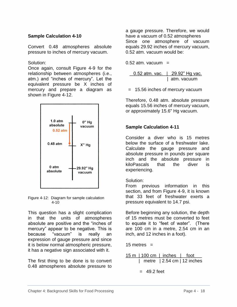
Chapter 4: Background Skills for Food Processing Page 4 - 18
Sample Calculation 4-10 Convert 0.48 atmospheres absolute pressure to inches of mercury vacuum. Solution: Once again, consult Figure 4-9 for the relationship between atmospheres (i.e., atm.) and “inches of mercury”. Let the equivalent pressure be X inches of mercury and prepare a diagram as shown in Figure 4-12.
Figure 4-12: Diagram for sample calculation 4-10
This question has a slight complication in that the units of atmospheres absolute are positive and the “inches of mercury” appear to be negative. This is because “vacuum” is really an expression of gauge pressure and since it is below normal atmospheric pressure, it has a negative sign associated with it. The first thing to be done is to convert 0.48 atmospheres absolute pressure to
a gauge pressure. Therefore, we would have a vacuum of 0.52 atmospheres Since one atmosphere of vacuum equals 29.92 inches of mercury vacuum, 0.52 atm. vacuum would be: 0.52 atm. vacuum = 0.52 atm. vac. | 29.92” Hg vac. | atm. vacuum | atm. vacuum = 15.56 inches of mercury vacuum Therefore, 0.48 atm. absolute pressure equals 15.56 inches of mercury vacuum, or approximately 15.6" Hg vacuum. Sample Calculation 4-11 Consider a diver who is 15 metres below the surface of a freshwater lake. Calculate the gauge pressure and absolute pressure in pounds per square inch and the absolute pressure in kiloPascals that the diver is experiencing. Solution: From previous information in this section, and from Figure 4-9, it is known that 33 feet of freshwater exerts a pressure equivalent to 14.7 psi. Before beginning any solution, the depth of 15 metres must be converted to feet to equate it to “feet of water”. (There are 100 cm in a metre, 2.54 cm in an inch, and 12 inches in a foot). 15 metres = 15 m | 100 cm | inches | foot . | metre | 2.54 cm | 12 inches = 49.2 feet
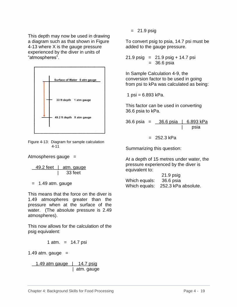
Chapter 4: Background Skills for Food Processing Page 4 - 19
This depth may now be used in drawing a diagram such as that shown in Figure 4-13 where X is the gauge pressure experienced by the diver in units of “atmospheres”.
Figure 4-13: Diagram for sample calculation 4-11
Atmospheres gauge = 49.2 feet | atm. gauge | 33 feet = 1.49 atm. gauge This means that the force on the diver is 1.49 atmospheres greater than the pressure when at the surface of the water. (The absolute pressure is 2.49 atmospheres). This now allows for the calculation of the psig equivalent: 1 atm. = 14.7 psi 1.49 atm. gauge = 1.49 atm gauge | 14.7 psig | atm. gauge
= 21.9 psig To convert psig to psia, 14.7 psi must be added to the gauge pressure. 21.9 psig = 21.9 psig + 14.7 psi = 36.6 psia In Sample Calculation 4-9, the conversion factor to be used in going from psi to kPa was calculated as being: 1 psi = 6.893 kPa. This factor can be used in converting 36.6 psia to kPa. 36.6 psia = 36.6 psia | 6.893 kPa | psia = 252.3 kPa Summarizing this question: At a depth of 15 metres under water, the pressure experienced by the diver is equivalent to: 21.9 psig Which equals: 36.6 psia Which equals: 252.3 kPa absolute.

Chapter 4: Background Skills for Food Processing Page 4 - 20
4.5.1 Practice Problems - Pressure 1. Convert 57 psig to “inches of
mercury absolute”. (Answer: 145.9 inches of mercury absolute)
2. Convert 29 psia to psig.
(Answer: 14.3 psig) 3. Convert 4.7 atm gauge to “bars”
gauge pressure. (Answer: 4.76 bars gauge)
4. A food processor has a heat
processing unit designed to run at an absolute pressure of 350 kPa. However, the instrument supplied by the manufacturer to indicate the pressure inside the unit was accidentally broken. A replacement pressure indicator identical to the original one cannot be found. Instead, it has to be replaced with one that indicates gauge pressures on two different scales. One is “inches of mercury gauge pressure” and the other is “psig”. What is the operating pressure on the basis of the two new scales? (Answer: 73.4 inches of mercury gauge, and 36.1 psig).
4.6 Density and Specific Gravity Food processors frequently work with large volumes of liquid solutions. Solutions of sugar in water, and various juice concentrates are typically used in the beverage-making industry. There are times when the processor must know the weight of sugar or other dissolved solids in a given volume of solution. This is especially true when putting together a number of ingredients for a batch of product. In most cases, the solids content of the solution is expressed on a weight basis and the volume is expressed in litres. For example, there may be 200 litres of a 40% by weight sugar solution in a tank and the operator needs to know the actual weight of sugar contained in that solution. While first instinct may say to simply multiply 200 litres by 40%, dimensional analysis indicates that it is not permissible to multiply or divide two values that do not have compatible units. Since weights are not measured in litres, 200 litres cannot be multiplied by 40% on a weight basis to get a meaningful answer. Before doing anything, the volume of 200 litres must be converted to a weight. This is done by means of its density. Density is a quantity that expresses the weight of a material per unit volume. By definition, one cubic centimetre of water at 4°C weighs one gram. This gives water a density of 1 gram per cubic centimetre. Since one cubic centimetre is defined as being one millilitre, the density of water can also be expressed as 1 gram per millilitre or one kilogram per litre. Once soluble solids are added to water, its density begins to change.
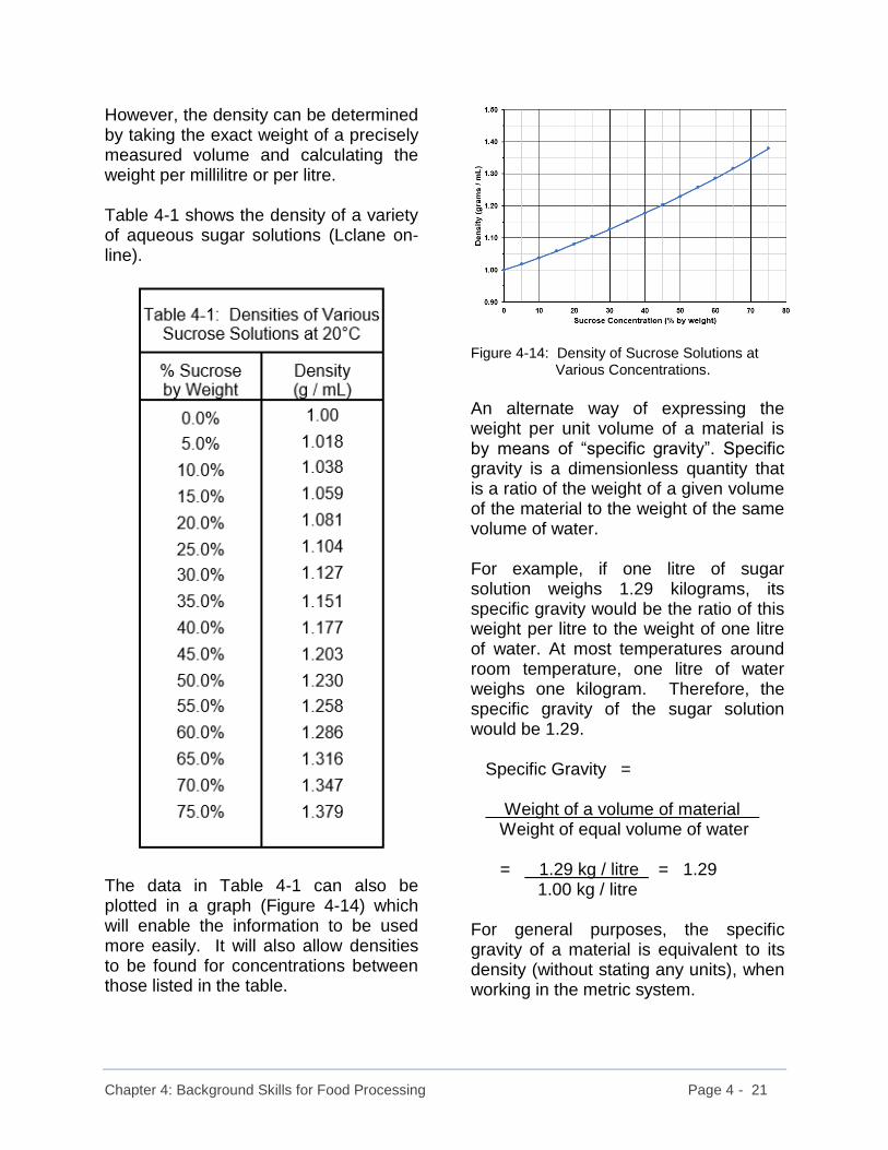
Chapter 4: Background Skills for Food Processing Page 4 - 21
However, the density can be determined by taking the exact weight of a precisely measured volume and calculating the weight per millilitre or per litre. Table 4-1 shows the density of a variety of aqueous sugar solutions (Lclane on-line).
The data in Table 4-1 can also be plotted in a graph (Figure 4-14) which will enable the information to be used more easily. It will also allow densities to be found for concentrations between those listed in the table.
Figure 4-14: Density of Sucrose Solutions at Various Concentrations.
An alternate way of expressing the weight per unit volume of a material is by means of “specific gravity”. Specific gravity is a dimensionless quantity that is a ratio of the weight of a given volume of the material to the weight of the same volume of water. For example, if one litre of sugar solution weighs 1.29 kilograms, its specific gravity would be the ratio of this weight per litre to the weight of one litre of water. At most temperatures around room temperature, one litre of water weighs one kilogram. Therefore, the specific gravity of the sugar solution would be 1.29. Specific Gravity = Weight of a volume of material . Weight of equal volume of water = 1.29 kg / litre = 1.29 1.00 kg / litre For general purposes, the specific gravity of a material is equivalent to its density (without stating any units), when working in the metric system.

Chapter 4: Background Skills for Food Processing Page 4 - 22
The most convenient aspect of specific gravity is that it allows the user to express the weight of material per unit volume in any appropriate set of units simply by multiplying the specific gravity by the density of water in those units. Table 4-2 lists the density of water in a variety of units. These conversions can be done using any convenient on-line density conversion application. Actual values may vary slightly but they will not make a significant difference in most food-related calculations.
Table 4-2 Density of Water in Various Units
(at 20°C)
1.0 gram per millilitre 1.0 kilogram per litre 1,000 kilograms per cubic metre 62.5 pounds per cubic foot 1,687.5 pounds per cubic yard 0.579 ounces per cubic inch 0.0362 pounds per cubic inch 10 pounds per Imperial gallon 8.344 pounds per U.S. gallon
Sample Calculation 4-12 Calculate the density of a sugar solution with a specific gravity of 1.29 in pounds per U.S. gallon. (Refer to Table 4-2). Solution: To calculate the weight of 1.0 U.S. gallon of the syrup, perform the following calculation: Density in “pounds per U.S. gallon” = density of water x Spec. Gravity in “lb per U.S. gallon” = 8.344 lb | 1.29 . U.S. gallon | = 10.76 lb / U.S. gallon Therefore, the sugar solution has a density of 10.76 pounds per U.S. gallon
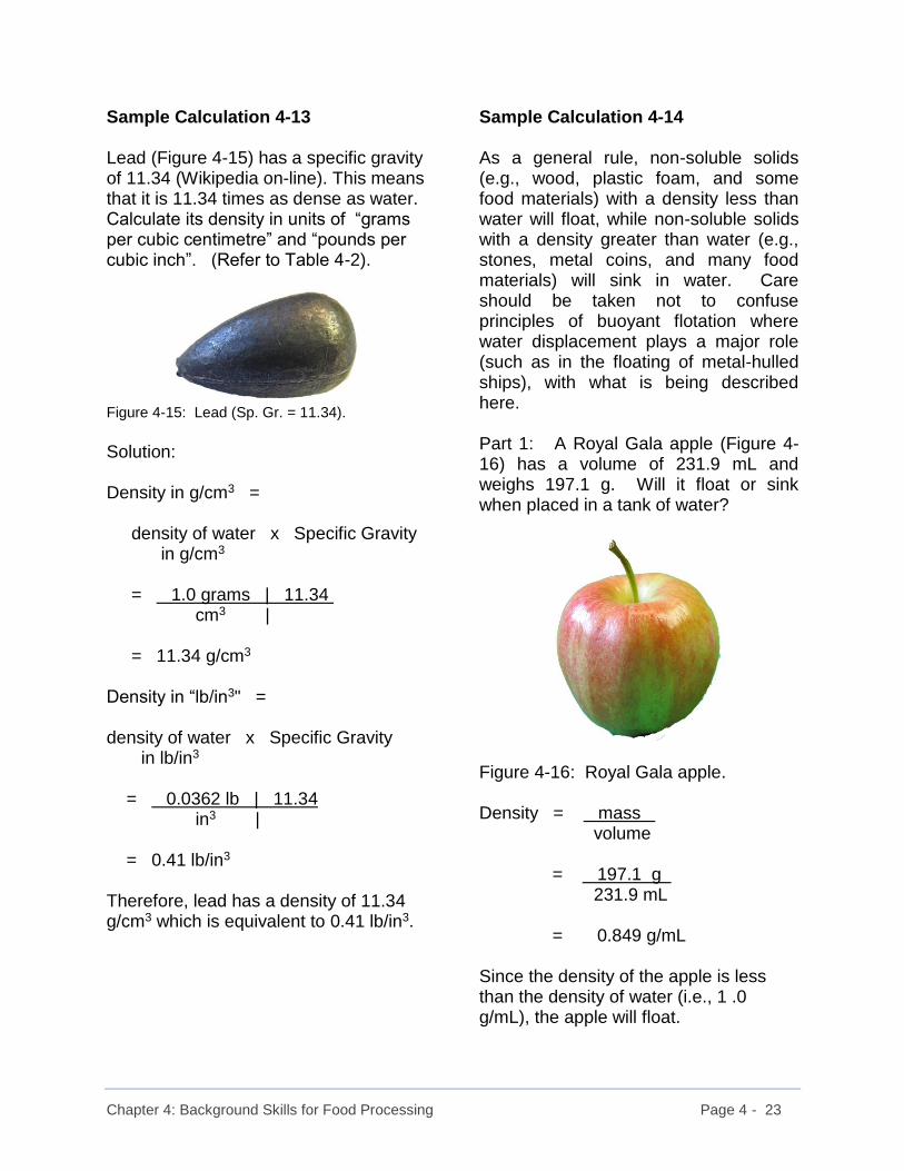
Chapter 4: Background Skills for Food Processing Page 4 - 23
Sample Calculation 4-13 Lead (Figure 4-15) has a specific gravity of 11.34 (Wikipedia on-line). This means that it is 11.34 times as dense as water. Calculate its density in units of “grams per cubic centimetre” and “pounds per cubic inch”. (Refer to Table 4-2).
Figure 4-15: Lead (Sp. Gr. = 11.34).
Solution: Density in g/cm3 = density of water x Specific Gravity in g/cm3 = 1.0 grams | 11.34 . cm3 | = 11.34 g/cm3 Density in “lb/in3" = density of water x Specific Gravity in lb/in3 = 0.0362 lb | 11.34 in3 | = 0.41 lb/in3 Therefore, lead has a density of 11.34 g/cm3 which is equivalent to 0.41 lb/in3.
Sample Calculation 4-14 As a general rule, non-soluble solids (e.g., wood, plastic foam, and some food materials) with a density less than water will float, while non-soluble solids with a density greater than water (e.g., stones, metal coins, and many food materials) will sink in water. Care should be taken not to confuse principles of buoyant flotation where water displacement plays a major role (such as in the floating of metal-hulled ships), with what is being described here. Part 1: A Royal Gala apple (Figure 4-16) has a volume of 231.9 mL and weighs 197.1 g. Will it float or sink when placed in a tank of water?
Figure 4-16: Royal Gala apple. Density = mass . volume = 197.1 g . 231.9 mL = 0.849 g/mL Since the density of the apple is less than the density of water (i.e., 1 .0 g/mL), the apple will float.

Chapter 4: Background Skills for Food Processing Page 4 - 24
Part 2: A small sample of white navy beans (Figure 4-17) weighing 47.73 grams was poured into a graduated cylinder containing 60.0 mL of water. The beans sank to the bottom of the cylinder. The volume of the beans and the water was 96.0 mL. What was the approximate density of the beans?
Figure 4-17: White navy beans.
Volume of beans = volume of beans - volume of water and water = 96.0 mL - 60.0 mL = 36.0 mL Density = mass . volume = 47.73 g 36.0 mL = 1.326 g/mL Therefore, the density of the white navy beans was approximately 1.33 g/mL. Since the beans sank, it should not be surprising that their density is greater than the density of water (i.e., 1.0 g/mL).
4.6.1 Determining Densities of Liquids Determining the density of liquids is a relatively straight-forward process and is not all that difficult with a few pieces of equipment (i.e., a graduated cylinder or similar measuring vessel and a scale or balance). Keeping in mind that the units of density are grams per mL, or kg per litre, we need to find the weight of a volume of the liquid. To do this, we can weigh a graduated cylinder when it is empty, then fill it with the liquid to a certain volume and weigh it again with the liquid in it. The difference between the weight of the cylinder when it is empty and the weight with the liquid in it will give us the weight of the liquid. The volume can be read directly from the lines on the side of the graduated cylinder. For more accurate measurements, a volumetric flask can be used. These flasks have been factory-calibrated to contain exactly their declared volume at the stated temperature. Dividing the weight of the liquid by its volume will give us the density.

Chapter 4: Background Skills for Food Processing Page 4 - 25
Sample Calculation 4-15 A previously weighed volumetric flask was filled to the calibration line with water (Figure 4-18). The filled flask was then weighed. The following results were obtained. Weight of empty flask = 82.50 g Weight of flask + water = 281.39 g Volume of water = 200.00 mL
Figure 4-18: Volumetric flask filled to calibration line with water. Colouring was added to the water for visual clarity.
Weight of water = Weight of flask - weight of empty + water flask = 281.39 g - 82.50 g = 198.89 g Density of water = weight / volume = 198.89 g / 200.00 mL = 0.994 g / mL
Therefore, the density of the water in this example is 0.994 g / mL, which is very close to 1.0 g / mL. When taking readings of liquids in flasks and cylinders, care must be taken to read the volume at the bottom of the curved surface or “meniscus” (Figure 4-19). This curvature is caused by surface tension.
Figure 4-19: The calibration line goes across the bottom of the meniscus for water.

Chapter 4: Background Skills for Food Processing Page 4 - 26
4.6.2 Determining Densities of Solids There are several ways to determine the density of solid materials. Once again, we need to find the weight and volume of a sample of the material in order to calculate its density. Method 1: Direct Measurement In this method, you can cut a cube of the material and measure its length, width, and height. Its volume can be found from the relationship: Volume = length x width x height = L x W x H Taking each of the measurements in centimetres (cm) will give the volume in cubic centimetres (cm3). Since one cubic centimetre is equal to one millilitre, the volume you calculate can be easily converted to millilitres (mL). You can weigh the sample on a balance to get its weight. Dividing the weight of the sample by its calculated volume will give its density.
Sample Calculation 4-16 In this example, a piece of potato was cut to approximate a cube (Figure 4-20). Its weight was recorded, and its three primary dimensions were measured with a set of electronic calipers.
Figure 4-20: “Cube” of potato for density determination.
Dimensions of potato sample: Length = 4.781 cm Width = 3.526 cm Height = 2.640 cm Weight = 46.80 g Volume = Length x Width x Height = 4.781 cm x 3.526 cm x 2.640 cm = 44.50 cm3 Since 1.0 cm3 = 1.0 mL, the volume of the potato sample is 44.50 mL. Density = Weight / Volume = 46.82 g / 44.50 mL = 1.052 g / mL Therefore, the density of the potato sample is approximately 1.05 g / mL.

Chapter 4: Background Skills for Food Processing Page 4 - 27
Method 2: Water Displacement Many materials are irregular in shape which makes it quite difficult to calculate their volume. In these cases, the water displacement method works extremely well. You can also cut appropriately sized chunks of material that will fit into your graduated cylinder. This should probably be the method used in most density determinations since it is easy to perform and may be more accurate than trying to prepare a cube of a sample and measure its three dimensions. First, you should put water in a graduated cylinder to about the half-way mark. Record the volume of the water and weigh the cylinder with the water in it. Now, place the sample of material in the graduated cylinder. If the material sinks, it is a simple matter to record the volume of the water and sample in the cylinder. If the sample floats, use the tip of a knife, or similar slender object (not your finger), to push the material completely below the surface. Record the volume of the sample and water in the cylinder. You can then place the graduated cylinder and its contents on your balance to get the total weight. Do not push the floating material under the water while you are taking the weight. This will create an error in the weight. The weight of the sample will be the weight of the cylinder with the water and sample inside minus the weight of the cylinder with only the water inside. The volume of the sample will be the volume of the contents of the cylinder
(i.e., the water and the sample) minus the volume of the water originally present in the cylinder. Dividing the weight of the sample by its calculated volume will give its density. Sample Calculation 4-17 In this calculation, a graduated cylinder containing 60.0 mL of water was weighed on an electronic balance. Then, several slices of potato (of suitable size to fit easily into the graduated cylinder) were dropped gently into the water. The weight of the graduated cylinder plus the water and the potato slices was recorded (Figure 4-21), as was the volume of the contents of the cylinder. Observed Data: Weight of cylinder + water = 177.09 g Weight of cylinder + water + sample = 205.67 g Volume of water at start = 60.0 mL Volume of water + sample = 86.5 mL Weight of sample = = weight of cylinder - weight of cylinder and contents and water = 205.67 g – 177.51 g = 28.58 g
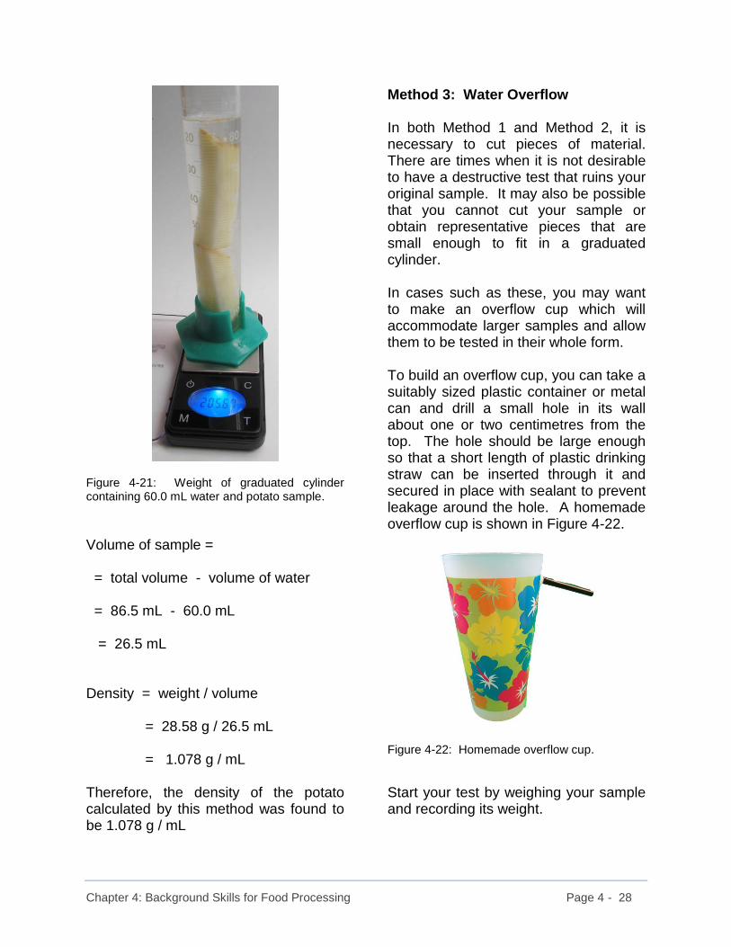
Chapter 4: Background Skills for Food Processing Page 4 - 28
Figure 4-21: Weight of graduated cylinder containing 60.0 mL water and potato sample.
Volume of sample = = total volume - volume of water = 86.5 mL - 60.0 mL = 26.5 mL Density = weight / volume = 28.58 g / 26.5 mL = 1.078 g / mL Therefore, the density of the potato calculated by this method was found to be 1.078 g / mL
Method 3: Water Overflow In both Method 1 and Method 2, it is necessary to cut pieces of material. There are times when it is not desirable to have a destructive test that ruins your original sample. It may also be possible that you cannot cut your sample or obtain representative pieces that are small enough to fit in a graduated cylinder. In cases such as these, you may want to make an overflow cup which will accommodate larger samples and allow them to be tested in their whole form. To build an overflow cup, you can take a suitably sized plastic container or metal can and drill a small hole in its wall about one or two centimetres from the top. The hole should be large enough so that a short length of plastic drinking straw can be inserted through it and secured in place with sealant to prevent leakage around the hole. A homemade overflow cup is shown in Figure 4-22.
Figure 4-22: Homemade overflow cup.
Start your test by weighing your sample and recording its weight.

Chapter 4: Background Skills for Food Processing Page 4 - 29
Set the overflow cup on the side of a sink with the drinking straw spout pointing over the sink. Fill the overflow cup with water to a level above the spout and allow the excess water to drain into the sink. Once the flow of water has stopped, you can begin your test to determine the volume of the material you have. Place a graduated cylinder in the sink under the overflow spout to catch the water that comes out. With the graduated cylinder in position, gently lower your sample into the cup. Do not drop the sample into the overflow cup, since this may cause the water in the cup to spill out over the top rim and ruin your test. Once the sample is almost submerged in the water, you can let go of it. Figure 4-23 shows the set-up before a sample has been placed in the overflow cup. For illustrative purposes, it has not been placed at the edge of a sink. You may need to hold the graduated cylinder up tight to the overflow tube to avoid spillage when doing the actual test.
Figure 4-23: Overflow cup set-up prior to running tests.
If the sample sinks, simply wait until the water stops flowing out the overflow spout and then record the volume in the graduated cylinder. If the sample floats, use a pointed knife, or similar object (not your finger), to push it below the surface. Hold the sample below the surface and wait until the water stops flowing out the overflow spout. You can then record the volume of the water collected. This will be the volume of your sample. You can now divide the weight of the sample by its volume to get the density. One problem that can be encountered in this test method is having a sample volume that is bigger than the volume of the graduated cylinder capacity. When this happens, the graduated cylinder will overflow and the test results will be meaningless. You may find it more convenient to collect the overflow water in a larger container. You can then measure the water volume by pouring it from the container into the graduated cylinder in several batches. Since the density of water at room temperature is very close to 1.00 grams per millilitre, you could weigh the container before and after collecting the overflow water. The difference in weight will be the weight of the water collected. This weight can then be converted to a volume (in mL). As already stated, you may have to lift the graduated cylinder so that the tip of the drinking straw spout on the overflow cup is pointing into it. This will avoid overflow water missing the cylinder as it leaves the spout.
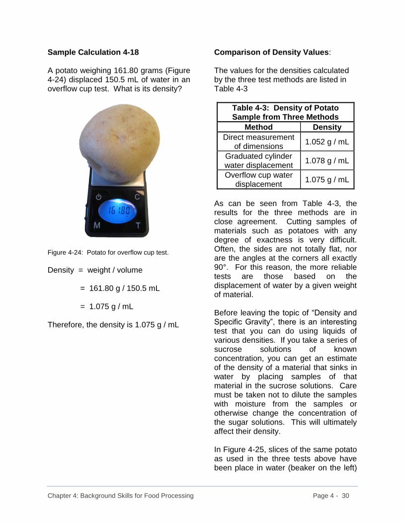
Chapter 4: Background Skills for Food Processing Page 4 - 30
Sample Calculation 4-18 A potato weighing 161.80 grams (Figure 4-24) displaced 150.5 mL of water in an overflow cup test. What is its density?
Figure 4-24: Potato for overflow cup test.
Density = weight / volume = 161.80 g / 150.5 mL = 1.075 g / mL Therefore, the density is 1.075 g / mL
Comparison of Density Values: The values for the densities calculated by the three test methods are listed in Table 4-3
Table 4-3: Density of Potato Sample from Three Methods
Method Density
Direct measurement of dimensions
1.052 g / mL
Graduated cylinder water displacement
1.078 g / mL
Overflow cup water displacement
1.075 g / mL
As can be seen from Table 4-3, the results for the three methods are in close agreement. Cutting samples of materials such as potatoes with any degree of exactness is very difficult. Often, the sides are not totally flat, nor are the angles at the corners all exactly 90°. For this reason, the more reliable tests are those based on the displacement of water by a given weight of material. Before leaving the topic of “Density and Specific Gravity”, there is an interesting test that you can do using liquids of various densities. If you take a series of sucrose solutions of known concentration, you can get an estimate of the density of a material that sinks in water by placing samples of that material in the sucrose solutions. Care must be taken not to dilute the samples with moisture from the samples or otherwise change the concentration of the sugar solutions. This will ultimately affect their density. In Figure 4-25, slices of the same potato as used in the three tests above have been place in water (beaker on the left)

Chapter 4: Background Skills for Food Processing Page 4 - 31
and a 50% by weight sucrose solution (beaker on the right). The density of water is 1.00 g / mL and the density of the 50% sucrose solution is 1.230 g / mL as indicated in Table 4-1. Since the density of the potato slice is greater than that of water, the potato will sink in water. In contrast, the density of the potato is considerably less than that of the 50% sucrose solution, so it will float in that solution. In both cases, blue food colouring has been added to the solutions for visual clarity.
Figure 4-25: A slice of potato sinks in water (left beaker) and floats in a 50% sucrose solution (right beaker) due to their density differences.
4.6.3 Practice Problems – Density and Specific Gravity 1. Calculate the weight of 500 litres of
solution with a specific gravity of 1.06. If the solids content is 16% by weight, what is the weight of solids present?
(Answer: 530 kg of solution containing 84.8 kg of solids)
2. A laboratory technician did a quick
experiment with a sample of sugar syrup in the lab. She accurately measured out 500 mL of syrup in a volumetric flask. The flask and its contents weighed 747.0 grams. The empty flask weighed 90.0 grams. What was the density and specific gravity of the syrup? Using Table 4-1 and comparing the density of this sugar syrup to the densities listed, what was the approximate percentage of sugar in the solution?
(Answer: Density = 1.314 g/mL or 1.314 kg/litre;
Specific Gravity = 1.314; Sugar content is approximately 65% sugar by weight).
3. What is the volume of 350 kg of a
solution of a 60% sucrose solution? Hint: You will need to use the information in Table 4-1. (Answer: 272.1 litres)

Chapter 4: Background Skills for Food Processing Page 4 - 32
4.7 Mass Balances Of all the calculations routinely performed in a food processing environment, one of the most beneficial is the “mass balance”. Mass balances are based on the principle that in any given process, the total weight of the materials leaving the process will equal the total weight of materials entering the process. To determine how much material might be lost as waste in a process, the total weight of product (excluding packaging material and the like) that is coming out of the process must be compared to the weight of all ingredients that were put into the process. Calculations of how much water has been removed from a product during a drying process can be accomplished by subtracting the weight of dried product coming out of the dryer from the weight of material entering the dryer. This assumes that there are no pieces of solid material lost in the dryer. An equally valid approach is to calculate the water contained in the material entering the dryer and subtract the amount of water in the product leaving the dryer. It is also possible to examine various streams leaving a process to determine the weights in each of them. In this way, individual sources of losses can be identified and the process can be adjusted to minimize these losses or eliminate them completely. The incentives for identifying process losses are very strong since losses reduce profitability and overall processing efficiencies.
In theory, mass balances are not difficult to perform. However, in practice, it is often difficult to get a reliable measurement of the streams leaving a process. For example, it may not be possible to determine how much product dust is leaving in the hot air travelling up the exhaust stack of a dryer. Similarly, reliable readings of the amount of solids being carried away in liquid waste streams are often difficult to obtain. In some cases, it may only be possible to identify the total losses from a process rather than the individual sources. Due to the fact that many processes involve the heating and cooling of materials, mass balances are often linked with “heat balances” in assessing how a process is performing. Heating and cooling, along with heat balances are discussed in the following chapter. It should also be noted that a knowledge of density and specific gravity is very helpful, since many mass balances require the conversion of liquid volume flowrates to mass flowrates. This can best be illustrated through a sample calculation.

Chapter 4: Background Skills for Food Processing Page 4 - 33
Sample Calculation 4-19 A processor is drying parsley flakes for use in the food industry. It is suspected that some pieces of dry parsley are being blown out of the dryer with the exhaust air (i.e., the air leaving the dryer). It is decided to do a mass balance on the process in an attempt to determine the size of these losses. In a test run, 375 kg of fresh parsley (at 85% moisture by weight) enter the dryer and 62.0 kg of dried parsley flakes with a moisture content of 12.0% (by weight) are collected at the other end of the dryer. What is the weight of dry solids (i.e., dried parsley) that has escaped with the exhaust air, if any? How much water is removed in the process? (Express your answer to one decimal place) Solution: Begin by drawing a diagram
as shown in Figure 4-26.
Figure 4-26: Diagram for drying mass balance.
The first thing to be done is to calculate the amount of water and solids entering the dryer as feed, and leaving the dryer as product. The difference between these quantities will be the amount of water and solids removed, respectively.
Calculations involving moisture content will be explained in much more detail in a later chapter. For now, we will express the water content of a material as its percent by weight without further elaboration. Weight of water “in” = weight of x fraction of parsley parsley “in” that is water = 375 kg x 0.85 = 318.75 kg Weight of solids “in” = weight of - weight of water “in” parley “in” = 375 kg - 318.75 kg = 56.25 kg Weight of water “out” = weight of x fraction of parsley parsley “out” that is water = 62.0 kg x 0.12 = 7.44 kg Weight of solids “out” = weight of - weight of water “out” parsley “out” = 62.0 kg - 7.44 kg = 54.56 kg

Chapter 4: Background Skills for Food Processing Page 4 - 34
Weight of solids lost = weight of - weight of solids “in” solids “out” = 56.25 kg - 54.56 kg = 1.69 kg Weight of water removed = weight of - weight of water “in” water “out” = 318.75 kg - 7.44 kg = 311.31 kg Therefore, 1.7 kg of dry parsley material are lost, and 311.3 kg of water are removed in the dryer. Sample Calculation 4-20 Costs of shipping food products from one location to another can be quite high. In order to reduce these costs, water is often removed from juices at their point of origin to reduce the shipping weight. The equivalent amount of water can then be re-added at the point of use or sale. This is typically what happens with orange juice and apple juice. The concentrate is placed in barrels and may be frozen prior to shipment to overseas markets. In this problem, we will consider a process to make orange juice concentrate. Water is removed from single strength juice with a solids content of 9.5% by weight to get a final product having 65% solids by weight. How much water would have to be
removed from 500 litres of freshly squeezed juice to obtain the desired concentrate? Calculate the weight of juice concentrate that would be obtained? Assume a specific gravity of 1.04 for the initial unconcentrated juice. Solution: Begin by drawing a diagram of the process to organize the available information. This will also assist in identifying what needs to be calculated and in determining any existing relationships between various masses flowing into and out of the process. See Figure 4-27.
Figure 4-27: Diagram for orange juice concentration problem.
In Figure 4-27, it can be seen that only water is being removed and no solids are lost in the concentration process. This leads to the relationship that the weight of solids leaving the process is identical to the weight of solids entering the process. Since the volume of juice entering the process is known, the first step is to convert the volume into a weight or mass. Once this is done, the weights of solids and water contained in the juice can be calculated.

Chapter 4: Background Skills for Food Processing Page 4 - 35
Total weight = volume x density of fresh juice Since the specific gravity of the juice is 1.04, its density would be 1.04 kg / litre (i.e., density of water times specific gravity of the juice) Total weight of fresh juice = 500 litres | 1.04 kg = 520 kg | litre Weight of solids = weight of juice x fraction of juice that is solids in fresh juice = 520 kg x 0.095 = 49.4 kg Note: 0.095 equals 9.5% as a decimal fraction Weight of water in fresh juice = weight of juice - weight of solids in fresh juice = 520 kg - 49.4 kg = 470.6 kg Because no solids are lost in the process, the juice concentrate will contain 49.4 kg of solids. Let “X kg” be the weight of the juice concentrate.
If there are 49.4 kg of solids present, then this represents 65% of the weight of the final juice concentrate. Therefore, 0.65 X = 49.4 kg Solving for “X” gives: X = 76.0 kg Weight of water in concentrate = weight of - weight of solids concentrate in concentrate = 76.0 kg - 49.4 kg = 26.6 kg Weight of water removed = weight of water - weight of water in fresh juice in concentrate = 470.6 kg - 26.6 kg = 444.0 kg Therefore, 444.0 kg of water must be removed and 76.0 kg of juice concentrate will be obtained.
Chapter 4: Background Skills for Food Processing Page 4 - 36
4.7 Practice Problems - Mass Balances
1. A fictitious powdered product
consists of a mixture of 10% sugar, 2% salt and 5% dried flavour ingredients, with the remainder being flour. How much flour is required to prepare 75 kg of the mixture? (Answer: 62.25 kg)
2. How much water must be
evaporated from 50 litres of a 10% by weight sugar solution to create a 40% by weight sugar syrup? How much syrup will be obtained? Hints: You will need to use Table 4-1 to obtain additional information for this problem. You should also calculate the amount of water at the start of this process and at the end of this process. (Answer: 39.0 kg of water must be removed and 13.0 kg of syrup will be obtained).
4.8 References
CAPGO. “History of Temperature”. On-line article available at: www.capgo.com/Resources/InterestStories/TempHistory/TempHistory.html (accessed March 2018). Personal knowledge also added to this section. Lclane. “Table - Sucrose Solutions, Composition, Viscosity, Density at 20°C”. Available on-line at: lclane.net/text/sucrose.html (accessed March 2018) Novo Industri A/S, Bagsvaerd, Denmark. “Novo’s Handbook of Practical Biotechnology”. A publication of the Bioindustrial Group, Edited by C.O.L. Boyce. Available in hard-copy, or for short-term on-line loan at: https://archive.org/details/novoshandbookofp00novo (accessed March 2018). Wikipedia. “Density of Lead”. Available on-line at: https://en.wikipedia.org/wiki/lead (accessed March 2018)
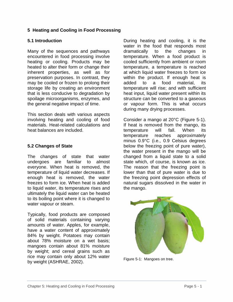
Chapter 5: Heating and Cooling in Food Processing Page 5 - 1
5 Heating and Cooling in Food Processing 5.1 Introduction Many of the sequences and pathways encountered in food processing involve heating or cooling. Products may be heated to alter their form or change their inherent properties, as well as for preservation purposes. In contrast, they may be cooled or frozen to prolong their storage life by creating an environment that is less conducive to degradation by spoilage microorganisms, enzymes, and the general negative impact of time. This section deals with various aspects involving heating and cooling of food materials. Heat-related calculations and heat balances are included. 5.2 Changes of State The changes of state that water undergoes are familiar to almost everyone. When heat is removed, the temperature of liquid water decreases. If enough heat is removed, the water freezes to form ice. When heat is added to liquid water, its temperature rises and ultimately the liquid water can be heated to its boiling point where it is changed to water vapour or steam. Typically, food products are composed of solid materials containing varying amounts of water. Apples, for example, have a water content of approximately 84% by weight. Potatoes may contain about 78% moisture on a wet basis; mangoes contain about 81% moisture by weight; and cereal grains such as rice may contain only about 12% water by weight (ASHRAE, 2002).
During heating and cooling, it is the water in the food that responds most dramatically to the changes in temperature. When a food product is cooled sufficiently from ambient or room temperature, a temperature is reached at which liquid water freezes to form ice within the product. If enough heat is added to a food material, its temperature will rise; and with sufficient heat input, liquid water present within its structure can be converted to a gaseous or vapour form. This is what occurs during many drying processes. Consider a mango at 20°C (Figure 5-1). If heat is removed from the mango, its temperature will fall. When its temperature reaches approximately minus 0.9°C (i.e., 0.9 Celsius degrees below the freezing point of pure water), the water present in the mango will be changed from a liquid state to a solid state which, of course, is known as ice. The reason that the freezing point is lower than that of pure water is due to the freezing point depression effects of natural sugars dissolved in the water in the mango.
Figure 5-1: Mangoes on tree.

Chapter 5: Heating and Cooling in Food Processing Page 5 - 2
When it first reaches -0.9°C, the water in the mango is still in its liquid state. However, as more heat is removed, the water will undergo a change of state to ice while the temperature remains constant at -0.9°C. Once the water is converted to ice crystals, any additional heat removal will cause the temperature of the now frozen mango to drop. If heat was added to the mango at 20°C, its temperature would begin to rise. Eventually, after enough heat was added, the temperature of the mango would stop rising and moisture would begin to leave the mango as water vapor. With the continual addition of heat, more and more water would be changed from a liquid to a gaseous state. However, the temperature of the mango would remain relatively constant in spite of this heat input. During the heating and cooling processes, there are two distinct effects that addition or removal of heat has on the mango. In one case, heat addition or removal creates a change in temperature of the mango. This heat is known as sensible heat since its effects can be sensed by the resultant temperature change. At the freezing point of the mango, the removal of heat does not create a temperature change. The effects of heat removal are not actually apparent as the water molecules go from being a liquid to becoming a solid, or ice. This heat is referred to as latent heat because its effects are hidden. When the mango is heated to the point where water evaporates without a change in temperature, latent heat is being added to change the water from its liquid to its gaseous state. This is the latent heat of vapourization.
With pure water, if the temperature is raised to its boiling point, the temperature will remain constant as water is vapourized. This is due to the latent heat of vapourization. Care must be taken when discussing the removal of water from any food material by vapourization. It is only the water that is vapourized. Food solids do not have a latent heat of vapourization since the solids making up the remainder of the material are not themselves vapourized. Further discussion of water removal by vapourization follows below. If the mango was at a temperature below its freezing point and heat was added, the mango’s temperature would rise to about -0.9°C. At this point, even with the addition of heat, the temperature would remain unchanged until the ice crystals had been converted to liquid water. After this, the temperature would continue to rise once again. The heat added or removed at the freezing point to change the state of water from a liquid to a solid, or from a solid to a liquid, is the latent heat of fusion. Approximately 270 kJ of heat must be removed from one kilogram of mangoes at their freezing point (i.e., -0.9°C) to convert the water present to ice. Similarly, 270 kJ of heat would have to be added to one kilogram of mangoes at their thawing temperature (i.e., -0.9°C) to change the ice within the mango to water in its liquid state.

Chapter 5: Heating and Cooling in Food Processing Page 5 - 3
5.3 Specific Heat The specific heat of a material is a measure of how much heat must be added or removed to create a one Celsius degree change in the temperature of one kilogram of that material. Water in its liquid state has a specific heat of 4.187 kJ/kg C°; which means that in order to change the temperature of one kilogram of water by one Celsius degree, 4.187 kiloJoules of heat must be added or removed. When water is frozen, the resultant ice has a specific heat of 2.050 kJ/kg C°. This means that 2.050 kiloJoules of heat must be added or removed to one kilogram of ice to change its temperature by one Celsius degree. To calculate the specific heat of a food material, Equation 5-1 can be applied.
The mass fraction of a component part of the material is its percentage expressed as a decimal fraction (Singh and Heldman, 2014). In the case of mangoes (Figure 5-2), the mass fraction of water would be 0.81 (81% water expressed as a decimal fraction). The remaining 19% of the mango is solid material, including sugar and fibre. This 19% becomes 0.19 and is the mass fraction of ash in the mango. Even though sugars may actually be a carbohydrate, they are treated as an “ash” component. “Carbohydrates” in this equation refers to starch materials rather than sugars.
Cp = 1.424 mc + 1.549 mp + 1.675 mf + 0.837 ma + 4.187 mw + 2.050 mi (Eq’n 5-1)
where: mc = mass fraction of carbohydrates mp = mass fraction of proteins mf = mass fraction of fat ma = mass fraction of ash mw = mass fraction of water mi = mass fraction of ice

Chapter 5: Heating and Cooling in Food Processing Page 5 - 4
Based on Equation 5-1, the specific heat of mangoes above their freezing point would be: Cp = 0.837 ma + 4.187 mw = (0.837 x 0.19 + 4.187 x 0.81) kJ / kg C°
= (0.159 + 3.391) kJ / kg C° = 3.550 kJ / kg C° Therefore, the specific heat of mangoes would be 3.550 kJ / kg C°, based on these calculations.
Figure 5-2: Mangoes have a specific heat of approximately 3.550 kJ / kg C°.
5.4 Latent Heat of Fusion The latent heat of fusion is the amount of heat that must be added to, or removed from, one kilogram of material at its freezing point to convert the water it contains from a liquid form to ice, or from a solid (i.e., ice) to a liquid. This is done with no change in temperature. Latent heat values may be found in literature sources. However, latent heats may not always be available for a specific food material. One method of determining an approximate latent heat of fusion value is to multiply the latent heat of fusion of pure water by the
weight fraction of water present in the material. This approach recognizes that it is only the water that actually freezes and goes through a transition from liquid to solid, or solid to liquid. The latent heat of fusion of pure water is 333.3 kJ / kg. Latent heat of fusion (approximate) = Latent heat of fusion x Mass fraction of pure water of water in material
(Eq’n 5-2) For example: Chicken (Figure 5-3) containing 74% moisture by weight would have a latent heat of fusion equal to 74% of the latent heat of fusion of water.
Figure 5-3: Chicken meat contains about 74% water by weight.
Latent heat of fusion of chicken = Latent heat of fusion x Mass fraction of pure water of water in the
chicken = 333.3 kJ / kg x 0.74
= 246.6 kJ / kg

Chapter 5: Heating and Cooling in Food Processing Page 5 - 5
From this it follows that 246.6 kJ of heat must be removed from 1 kg of chicken at its freezing point (i.e., -2.8°C) to change the water it contains from a liquid form to ice. Similarly, 246.6 kJ of heat would have to be added to thaw 1 kg of chicken at its freezing point. In comparison: The latent heat of fusion of tomatoes Figure 5-4) containing 94% moisture would be: Latent heat of fusion of tomatoes = Latent heat of fusion x mass fraction of pure water of water in the
tomatoes = 333.3 kJ / kg x 0.94 = 313.3 kJ / kg Therefore, the latent heat of fusion of tomatoes is 313.3 kJ/kg.
Figure 5-4: Tomatoes may contain 94% to 95% water by weight.
5.5 Calculations of Heat Addition and Heat Removal In order to calculate the amount of heat that must be added or removed from a given mass (i.e., weight) of material to create a given change in temperature, the following equation can be used: Heat = m Cp ΔT (Eq’n 5-3) where: m = mass of material (kg) Cp = specific heat (kJ / kg C°) ΔT = change in temperature
(Celsius degrees) If the food material is being frozen or thawed, it is necessary to calculate the amount of heat required for the actual change of state of the water present. This can be done by means of the following equation: Heat = Latent Heat of Fusion x mass (Eq’n 5-4) Table 5-1 presents information which can be used in heating and cooling calculations for a number of products. It is important to note that the specific heat for the frozen material is different from that of the material above its freezing point. The information in Table 5-1 will be used in the sample problems that follow.
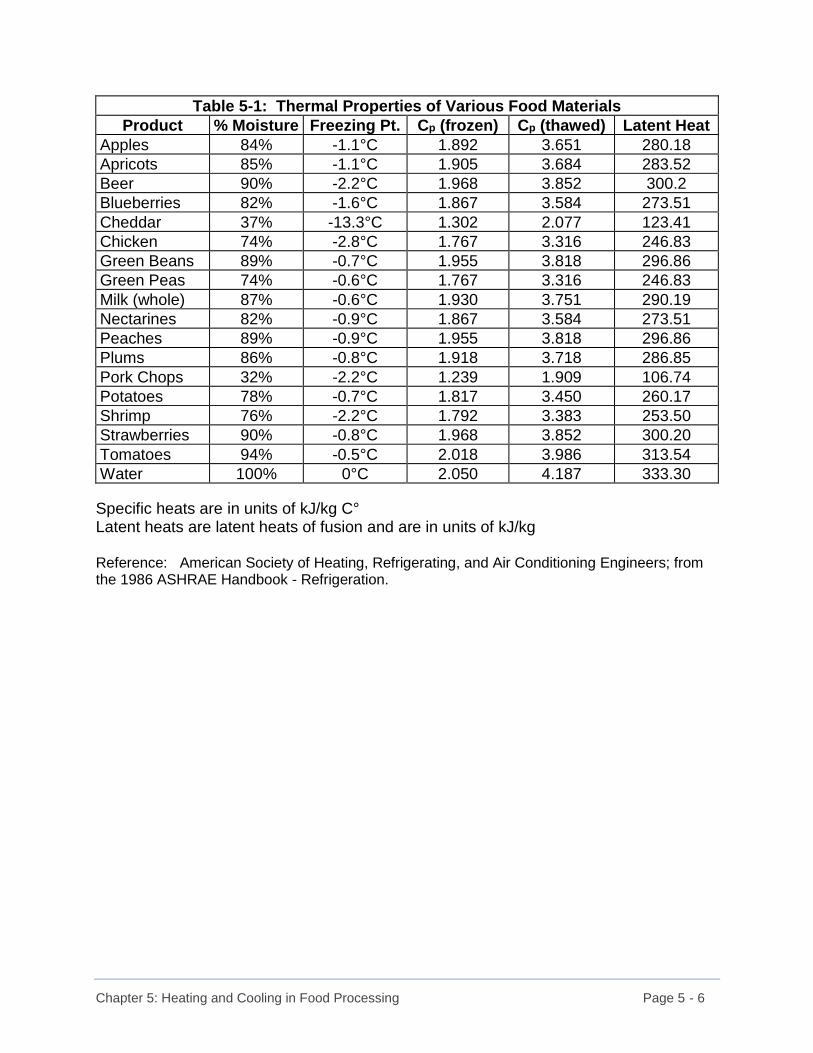
Chapter 5: Heating and Cooling in Food Processing Page 5 - 6
Table 5-1: Thermal Properties of Various Food Materials
Product % Moisture Freezing Pt. Cp (frozen) Cp (thawed) Latent Heat
Apples 84% -1.1°C 1.892 3.651 280.18
Apricots 85% -1.1°C 1.905 3.684 283.52
Beer 90% -2.2°C 1.968 3.852 300.2
Blueberries 82% -1.6°C 1.867 3.584 273.51
Cheddar 37% -13.3°C 1.302 2.077 123.41
Chicken 74% -2.8°C 1.767 3.316 246.83
Green Beans 89% -0.7°C 1.955 3.818 296.86
Green Peas 74% -0.6°C 1.767 3.316 246.83
Milk (whole) 87% -0.6°C 1.930 3.751 290.19
Nectarines 82% -0.9°C 1.867 3.584 273.51
Peaches 89% -0.9°C 1.955 3.818 296.86
Plums 86% -0.8°C 1.918 3.718 286.85
Pork Chops 32% -2.2°C 1.239 1.909 106.74
Potatoes 78% -0.7°C 1.817 3.450 260.17
Shrimp 76% -2.2°C 1.792 3.383 253.50
Strawberries 90% -0.8°C 1.968 3.852 300.20
Tomatoes 94% -0.5°C 2.018 3.986 313.54
Water 100% 0°C 2.050 4.187 333.30
Specific heats are in units of kJ/kg C° Latent heats are latent heats of fusion and are in units of kJ/kg Reference: American Society of Heating, Refrigerating, and Air Conditioning Engineers; from the 1986 ASHRAE Handbook - Refrigeration.
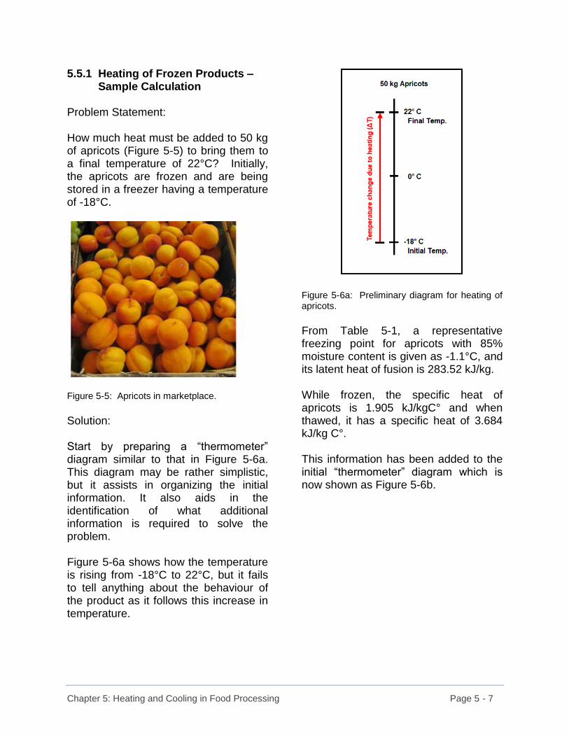
Chapter 5: Heating and Cooling in Food Processing Page 5 - 7
5.5.1 Heating of Frozen Products – Sample Calculation Problem Statement: How much heat must be added to 50 kg of apricots (Figure 5-5) to bring them to a final temperature of 22°C? Initially, the apricots are frozen and are being stored in a freezer having a temperature of -18°C.
Figure 5-5: Apricots in marketplace.
Solution: Start by preparing a “thermometer” diagram similar to that in Figure 5-6a. This diagram may be rather simplistic, but it assists in organizing the initial information. It also aids in the identification of what additional information is required to solve the problem. Figure 5-6a shows how the temperature is rising from -18°C to 22°C, but it fails to tell anything about the behaviour of the product as it follows this increase in temperature.
Figure 5-6a: Preliminary diagram for heating of apricots.
From Table 5-1, a representative freezing point for apricots with 85% moisture content is given as -1.1°C, and its latent heat of fusion is 283.52 kJ/kg. While frozen, the specific heat of apricots is 1.905 kJ/kgC° and when thawed, it has a specific heat of 3.684 kJ/kg C°. This information has been added to the initial “thermometer” diagram which is now shown as Figure 5-6b.
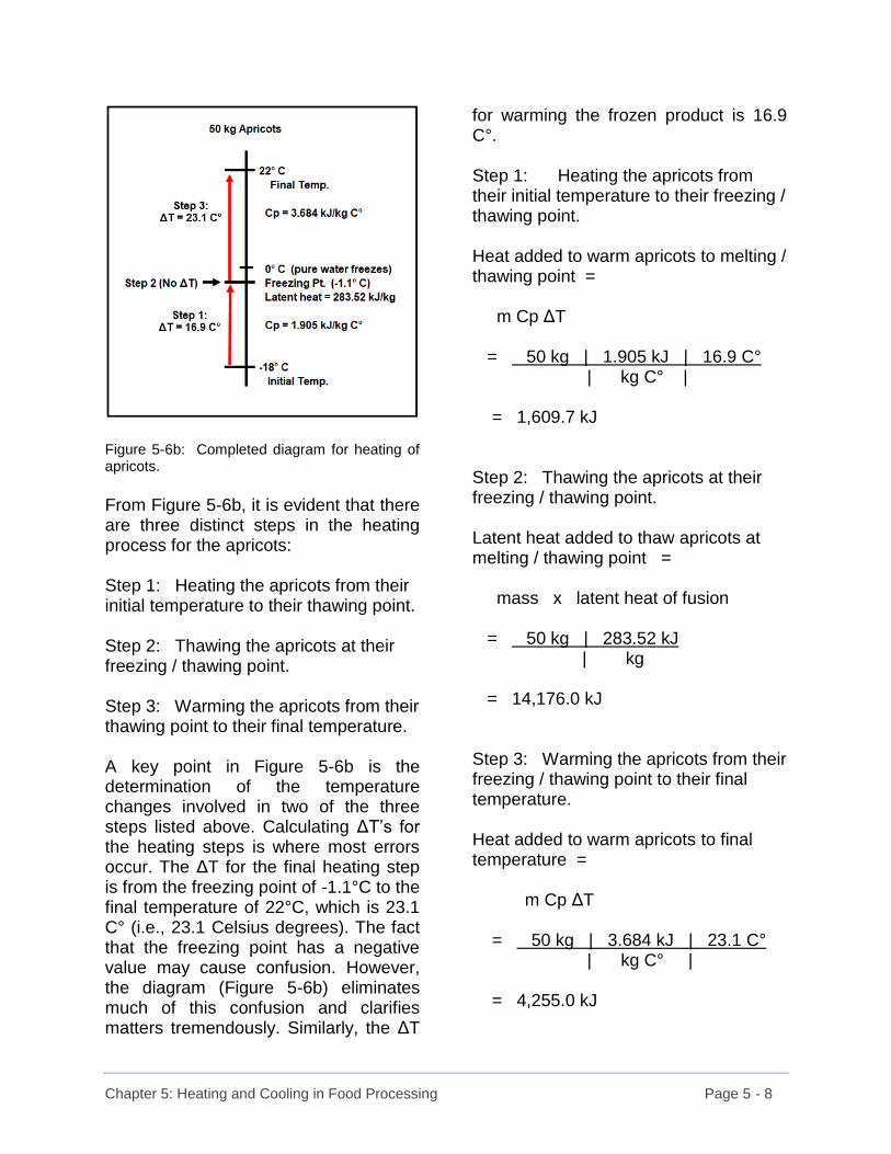
Chapter 5: Heating and Cooling in Food Processing Page 5 - 8
Figure 5-6b: Completed diagram for heating of apricots.
From Figure 5-6b, it is evident that there are three distinct steps in the heating process for the apricots: Step 1: Heating the apricots from their initial temperature to their thawing point. Step 2: Thawing the apricots at their freezing / thawing point. Step 3: Warming the apricots from their thawing point to their final temperature. A key point in Figure 5-6b is the determination of the temperature changes involved in two of the three steps listed above. Calculating ΔT’s for the heating steps is where most errors occur. The ΔT for the final heating step is from the freezing point of -1.1°C to the final temperature of 22°C, which is 23.1 C° (i.e., 23.1 Celsius degrees). The fact that the freezing point has a negative value may cause confusion. However, the diagram (Figure 5-6b) eliminates much of this confusion and clarifies matters tremendously. Similarly, the ΔT
for warming the frozen product is 16.9 C°. Step 1: Heating the apricots from their initial temperature to their freezing / thawing point. Heat added to warm apricots to melting / thawing point = m Cp ΔT = 50 kg | 1.905 kJ | 16.9 C° | kg C° | = 1,609.7 kJ Step 2: Thawing the apricots at their freezing / thawing point. Latent heat added to thaw apricots at melting / thawing point = mass x latent heat of fusion = 50 kg | 283.52 kJ | kg = 14,176.0 kJ Step 3: Warming the apricots from their freezing / thawing point to their final temperature. Heat added to warm apricots to final temperature = m Cp ΔT = 50 kg | 3.684 kJ | 23.1 C° | kg C° | = 4,255.0 kJ

Chapter 5: Heating and Cooling in Food Processing Page 5 - 9
Final Calculation: Total heat to be added = total of heat from each of the three steps = heat added + heat added + heat added in step 1 in step 2 in step 3 = 1,609.7 kJ + 14,176.0 kJ + 4,255.0 kJ = 20,040.7 kJ
Therefore, it takes approximately 20,041 kJ to heat the frozen apricots to their final temperature. This value may be rounded off to 20,000 kJ since all calculations of this type are basically approximations. 5.5.2 Freezing of Products – Sample Calculation Problem Statement: How much heat must be removed from 35 kg of pork chops (Figure 5-7) if they are at an initial temperature of 50°F and must be frozen to a final temperature of -25°C ?
Figure 5-7: Sides of pork in chilled room.
Solution: Start by converting the Fahrenheit temperature to the desired Celsius equivalent. The procedure for doing this conversion is discussed in the “Background Skills for Food Processing” chapter (i.e., Chapter 4). 50°F = [(50 - 32) / 1.8 ] °C
= [ 18 / 1.8 ] °C = 10.0°C
It is now possible to prepare an initial “thermometer” diagram as was done in the previous example. Figure 5-8a is incomplete since it omits information about the change from the thawed to frozen state, as well as values needed for the various calculations.
Figure 5-8a: Preliminary diagram for the freezing of pork chops.
Once again, the required information can be found in Table 5-1. Figure 5-8b shows the completed diagram for this problem.

Chapter 5: Heating and Cooling in Food Processing Page 5 - 10
Figure 5-8b: Completed diagram for freezing of pork chops.
From Figure 5-8b, the three distinct steps for the freezing of the pork chops can be identified: Step 1: Cooling the pork chops to their freezing point. Step 2: Freezing the pork chops at their freezing point. Step 3: Cooling the frozen pork chops to their final temperature. BEWARE: In dealing with temperature changes, it is best to maintain a positive value for the ΔT’s rather than having negative values for them. This reduces a lot of confusion and error. While it is absolutely correct from a thermodynamic standpoint to have negative ΔT’s to show that heat is lost,
students in my classes often forget that the latent heat of fusion term is also a negative value when removing heat or cooling a material. They then add a positive latent heat and two negative heats for the temperature changes and get an incorrect answer. Instead of using a negative sign to show heat being given up by the material in cooling, use of wording such as “heat removed from the material” or “heat lost by the material” is a much safer option. Although experts in thermodynamics may disagree, this approach creates a more thorough understanding of what is happening with fewer errors in the calculations. It is also beneficial to think of the procedures in the same manner in which you would speak of them in your normal conversation. While it is perfectly acceptable to say that something has a negative enthalpy (i.e., the heat flow is out of the material). It is easier to understand someone when they say that the material has a certain amount of heat loss or heat removal.
Step 1: Cooling the pork chops from their initial temperature to their freezing point. Heat removed to cool pork chops to their freezing point = m Cp ΔT = 35 kg | 1.909 kJ | 12.2 C° | kg C° | = 815.1 kJ

Chapter 5: Heating and Cooling in Food Processing Page 5 - 11
Step 2: Freezing the pork chops at their freezing point. Latent heat removed to freeze pork chops at freezing point = mass x latent heat of fusion = 35 kg | 106.74 kJ | kg = 3,735.9 kJ Step 3: Cooling the frozen pork chops to their final temperature. Heat removed to cool pork chops to their final temperature from freezing point = m Cp ΔT = 35 kg | 1.239 kJ | 22.8 C° | kg C° | = 988.7 kJ Final Calculation: Total heat to be removed = total of heat from each of the three steps = Step 1 + Step 2 + Step 3 = 815.1 kJ + 3,735.9 kJ + 988.7 kJ = 5,539.7 kJ Therefore, approximately 5,540 kJ of heat must be removed from the 35 kg of pork chops to cool and freeze them.
5.5.3 Practice Problems 1. A peach grower harvests 2,550 kg of
peaches on a relatively warm day when the temperature is 27°C. The grower realizes that to reduce the risk of spoilage, the temperature of the peaches should be brought down as soon as possible. He also knows that peaches (Figure 5-9) are highly sensitive to freezing injury, so the optimal temperature would be approximately 4°C. How much heat would have to be removed to accomplish the desired temperature change for the harvested peaches?
Figure 5-9: Peaches are very susceptible to
spoilage after harvesting.
Answer: approximately 223,926 kJ
of heat must be removed

Chapter 5: Heating and Cooling in Food Processing Page 5 - 12
2. A small-scale brewery needs to cool a number of batches of beer from a fermentation temperature of 69°F to a final temperature of 33°F. In order to match the cooling capacity of the chilling process, the beer is cooled at a rate of 325 kg per hour. What is the rate of heat removal (expressed in kJ per hour)? What quantity of heat is removed during a 12 hour processing run?
Note: Convert the temperatures to
Celsius before starting to solve the problem.
Answer: Heat removal rate is 25,038 kJ / hour Heat removed in 12 hours is 300,456
kJ 3. A processor is preparing apple
sauce that will be frozen after it is made. 350 kg of cleaned cored apples are heated from an initial storage temperature of 4°C to 98°C and held at this temperature until the desired texture is achieved. The apple sauce (Figure 5-10) is then cooled to approximately 20°C and packaged in plastic containers prior to freezing. The frozen apple sauce is kept at -18°C. How much heat must be added in the cooking step and how much heat must be removed in the freezing process. What assumptions are being made about this process.
Figure 5-10: Apple sauce.
Answers: Approximately 120,118 kJ of heat
are required to heat the apples. Approximately 235,890 kJ of heat
must be removed in the freezing process. (The 20°C packaging temperature is not important in the overall heat calculations).
It is assumed that the process is
100% efficient and that no heat or water are lost to the surroundings etc. This is generally not the case in actual processing operations since heat is lost through the surfaces of the equipment and water vapour may also escape from the process. It is also assumed that the specific heat of the pieces of apples is the same as that of an entire apple. Such an assumption would be reasonable under these conditions.
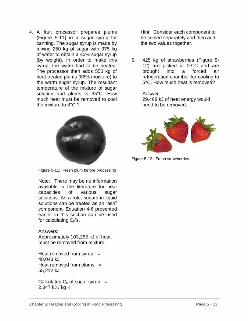
Chapter 5: Heating and Cooling in Food Processing Page 5 - 13
4. A fruit processor prepares plums (Figure 5-11) in a sugar syrup for canning. The sugar syrup is made by mixing 250 kg of sugar with 375 kg of water to obtain a 40% sugar syrup (by weight). In order to make this syrup, the water had to be heated. The processor then adds 550 kg of heat treated plums (86% moisture) to the warm sugar syrup. The resultant temperature of the mixture of sugar solution and plums is 35°C. How much heat must be removed to cool the mixture to 8°C ?
Figure 5-11: Fresh plum before processing
Note: There may be no information
available in the literature for heat capacities of various sugar solutions. As a rule, sugars in liquid solutions can be treated as an “ash” component. Equation 4-6 presented earlier in this section can be used for calculating Cp’s.
Answers: Approximately 103,255 kJ of heat
must be removed from mixture. Heat removed from syrup =
48,043 kJ Heat removed from plums =
55,212 kJ Calculated Cp of sugar syrup =
2.847 kJ / kg K
Hint: Consider each component to be cooled separately and then add the two values together.
5. 425 kg of strawberries (Figure 5-
12) are picked at 23°C and are brought into a forced air refrigeration chamber for cooling to 5°C. How much heat is removed?
Answer: 29,468 kJ of heat energy would
need to be removed.
Figure 5-12: Fresh strawberries.

Chapter 5: Heating and Cooling in Food Processing Page 5 - 14
5.6 Steam as a Heat Source Many industrial processes utilize steam for heating their products. High pressure steam is produced in boilers in a steam plant and is then piped to various locations around the food processing facility. The high pressure steam usually goes through one or more pressure reducing steps before it is used. Typically, its pressure would be 50 pounds per square inch or less (i.e., 50 psi or less) as the steam enters as processing area and then it may be reduced further to suit the requirements of individual pieces of equipment. In thermodynamics and heat-related problems, quantities of steam are often expressed on a weight basis. One kilogram of steam is the amount of steam produced by completely vapourizing one kilogram of water (Figure 5-13).
Figure 5-13: It takes 2,257.1 kJ of heat to convert 1.0 kg of water to 1.0 kg of vapour at atmospheric pressure.
For discussion purposes, consider an autoclave used to sterilize media for a microbiology lab or to sterilize medical tools (Figure 5-14).
Figure 5-14: Autoclave used for sterilizing laboratory equipment. Closed in upper photo and open in lower photo.
Steam supplied to the autoclave is kept at approximately 1 atmosphere gauge pressure. At this pressure, the steam has a temperature of 120°C and contains about 2,706.3 kilojoules of heat per kilogram of steam.
The steam in our sample problem at 120°C can be kept above atmospheric pressure and allowed to condense. This will give liquid water or “condensate” at 120°C. During the process of the vapour changing to liquid condensate, most of the heat originally contained in the steam is released.
The hot condensate under pressure at 120°C contains about 503.7 kilojoules of heat per kilogram. The heat released in condensing one kilogram of steam under these conditions can be calculated as:

Chapter 5: Heating and Cooling in Food Processing Page 5 - 15
Heat released in = heat contained in - heat contained in condensing 1 kg 1 kg of vapour 1 kg of condensate of steam These quantities of heat are often referred to as “enthalpy”, where the enthalpy is the amount of heat expressed in units of kiloJoules per kilogram (i.e., kJ/kg). Using “h” as an abbreviation for enthalpy and the subscripts “v” and “c” for “vapour” and “condensate respectively, the relationship above can be re-written as: h = hv - hc (Eq’n 5-10) To calculate the amount of heat released when 1 kg of steam at 200 kPa is condensed, the values of the enthalpies given for the autoclave example can be used. h = hv - hc = 2,706.3 kJ / kg - 503.7 kJ / kg = 2,202.6 kJ / kg Therefore, approximately 2,203 kJ of heat are obtained when one kilogram of steam at this pressure is condensed.
Detailed tables giving information about the heat content of steam under various pressures are available in the literature. Table 5-2 lists enthalpy values of steam at several different pressures, as well as the corresponding temperature of the steam. Steam in which all of the water is present as vapour is referred to as “saturated steam”. If water droplets are present in the steam, then it is not saturated and has a lower heat content. Only saturated steam is being considered here.

Chapter 5: Heating and Cooling in Food Processing Page 5 - 16
Table 5-2: Heat Values for Saturated Steam at Various Pressures
Temperature (°C)
Pressure (kPa gauge)
Pressure (psig)
Vapour Enthalpy (kJ/kg)
Condensate Enthalpy (kJ/kg)
50 12.3 1.8 2,592.1 209.3
60 19.9 2.9 2,609.6 251.1
70 31.2 4.5 2,626.8 293.0
80 47.4 6.9 2,643.7 334.9
90 70.1 10.2 2,660.1 376.9
100 101.3 14.7 2,676.1 419.0
110 143.3 20.8 2,691.5 461.3
120 198.5 28.8 2,706.3 503.7
130 270.1 39.2 2,720.5 546.3
140 316.3 45.9 2,733.9 589.1
150 475.8 69.0 2,746.5 632.2
Ref: Selected values for steam over a range of temperatures have been taken from various steam table sources. In some processes, heat is not only obtained by condensing the steam, but also by cooling the hot condensate. For example, if the condensate gathered from condensing steam at 120°C was cooled to 70°C, its enthalpy would drop from 503.7 kJ/kg to 293.0 kJ/kg. The result would be that 210.7 kJ of additional heat could be recovered from each kilogram of condensate, essentially from each kilogram of steam that is condensed. In an industrial heating process, steam can introduced into a “jacket” around the outside of a tank. Basically, a jacketed tank has double walls with a space between them to allow the steam to pass. As steam condenses inside the jacket (see Figure 5-15), it releases its latent heat. The heat is then transmitted through the walls of the tank and warms the contents. Since heat also passes through the outer walls of the jacket and
is lost to the surrounding air, tanks may be insulated to reduce heat loss.
Figure 5-15: Using steam as a heat source in a jacketed tank or kettle.

Chapter 5: Heating and Cooling in Food Processing Page 5 - 17
5.6.1 Sample Steam Calculations Problem Statement 5-1 How much saturated steam at 270.1 kPa pressure does it take to heat 200 kg of blueberries (Figure 5-16) from 4°C to 90°C? Usually, berries are mashed for heating processes. Express the answer in kilograms of steam and assume that no heat is lost in the process.
Figure 5-16: Blueberries before mashing.
Solution: The heat required to warm the blueberries must be calculated first. The specific heat for blueberries can be obtained from Table 4-3. A diagram can now be prepared as shown in Figure 5-17.
Figure 5-17: Diagram for heating of blueberries.
Heat required = m Cp ΔT = 200 kg | 3.584 kJ | 86 C° | kg C° | = 61,645 kJ The heat released by condensing a kilogram of saturated steam at 270.1 kPa can be determined. h = hv - hc = 2,720.5 kJ / kg - 546.3 kJ / kg = 2,174.2 kJ / kg Weight of steam required = heat required . amount of heat per kg steam = 61,645 kJ | kg steam | 2,174.2 kJ = 28.4 kg steam Therefore, 28.4 kg of steam at 270.1 kPa pressure are required.

Chapter 5: Heating and Cooling in Food Processing Page 5 - 18
Problem Statement 5-2 How much steam would be required to process the blueberries in the previous example if the condensate was allowed to cool to 80°C during the heat exchange process, and no heat is lost to the surroundings? Calculate the difference between this process and the previous one where heat was not recovered from the condensate. Solution: The amount of heat to warm the blueberries remains unchanged at 61,645 kJ. The enthalpy of the steam in its vapour form (hv) at 270.1 kPa is 2,720.5 kJ/kg steam However, the enthalpy of the condensate (hc) is now the enthalpy of condensate at 80°C, which is 334.9 kJ/kg. Heat obtained = enthalpy of steam as - enthalpy of vapour at 270.1 kPa condensate at 80°C h = hv - hc = 2,720.5 kJ / kg - 334.9 kJ / kg = 2,385.6 kJ / kg
Weight of steam required = heat required . amount of heat per kg steam = 61,645 kJ | kg steam | 2,385.6 kJ = 25.8 kg steam Therefore, 25.8 kg of steam at 270.1 kPa pressure are required when heat is also recovered by cooling the condensate. When no heat was recovered from the condensate, 28.4 kg of steam were required. With heat recovery from the condensate, 2.6 kg less steam are required than when heat is not recovered from the condensate (i.e., 28.4 kg - 25.8 kg steam).

Chapter 5: Heating and Cooling in Food Processing Page 5 - 19
Problem Statement 5-3 Calculate the amount of steam required in the blueberry process with heat recovery from the condensate (previous example) if 35% of the heat supplied to the process was lost to the surroundings. Solution: Two approaches could be used to solve this problem. In the first approach, it could be said that 25.8 kg of steam are required to supply the needs of the process in raising the temperature of the blueberries. Since 35% of the heat is lost, the amount of heat actually used is 65% of the total amount that must be supplied to the process. In other words, the efficiency of the process is 65% on the basis of heat utilization. Therefore, 65% of the total heat supplied must equal 61,645 kJ which came from 25.6 kg of steam. Letting X be the weight of the steam that must be supplied to the process, 0.65 X = 25.8 kg steam Solving for X: X = 39.7 kg steam Therefore, approximately 39.7 kg of steam must be supplied to the process to account for heat losses and to do the heating of the blueberries.
The second approach would be to recognize that 65% of the heat goes into heating the blueberries. Letting Y be the total amount of heat that must be supplied, 0.65 Y = 61,645 kJ Solving for Y: Y = 94,838 kJ Since each kg of steam that condenses and has its condensate cooled to 80°C provides 2,385.6 kJ of heat, it follows: Weight of steam required = 94,838 kJ | kg steam
| 2,385.6 kJ = 39.7 kg steam Therefore, 39.7 kg of steam would be required for this process. It should be noted that the amounts of steam calculated by these two approaches may differ slightly in the second decimal place. This can be attributed to round-off in the previous calculations.
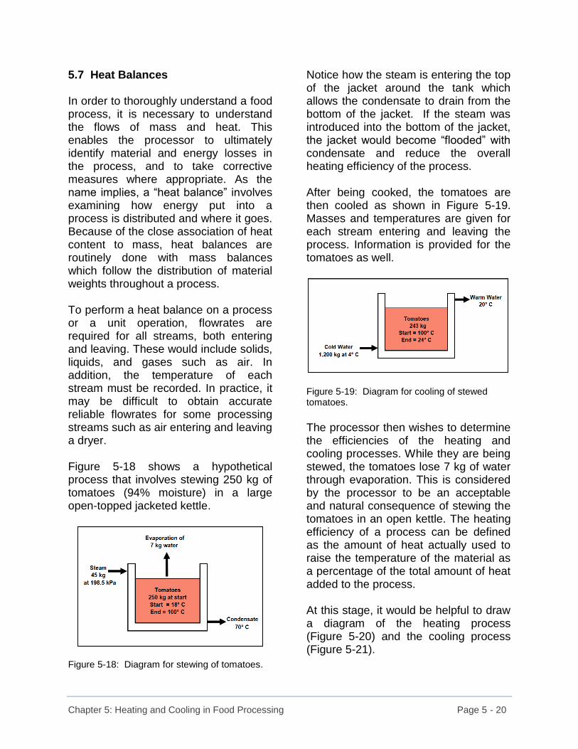
Chapter 5: Heating and Cooling in Food Processing Page 5 - 20
5.7 Heat Balances In order to thoroughly understand a food process, it is necessary to understand the flows of mass and heat. This enables the processor to ultimately identify material and energy losses in the process, and to take corrective measures where appropriate. As the name implies, a “heat balance” involves examining how energy put into a process is distributed and where it goes. Because of the close association of heat content to mass, heat balances are routinely done with mass balances which follow the distribution of material weights throughout a process. To perform a heat balance on a process or a unit operation, flowrates are required for all streams, both entering and leaving. These would include solids, liquids, and gases such as air. In addition, the temperature of each stream must be recorded. In practice, it may be difficult to obtain accurate reliable flowrates for some processing streams such as air entering and leaving a dryer. Figure 5-18 shows a hypothetical process that involves stewing 250 kg of tomatoes (94% moisture) in a large open-topped jacketed kettle.
Figure 5-18: Diagram for stewing of tomatoes.
Notice how the steam is entering the top of the jacket around the tank which allows the condensate to drain from the bottom of the jacket. If the steam was introduced into the bottom of the jacket, the jacket would become “flooded” with condensate and reduce the overall heating efficiency of the process. After being cooked, the tomatoes are then cooled as shown in Figure 5-19. Masses and temperatures are given for each stream entering and leaving the process. Information is provided for the tomatoes as well.
Figure 5-19: Diagram for cooling of stewed tomatoes.
The processor then wishes to determine the efficiencies of the heating and cooling processes. While they are being stewed, the tomatoes lose 7 kg of water through evaporation. This is considered by the processor to be an acceptable and natural consequence of stewing the tomatoes in an open kettle. The heating efficiency of a process can be defined as the amount of heat actually used to raise the temperature of the material as a percentage of the total amount of heat added to the process. At this stage, it would be helpful to draw a diagram of the heating process (Figure 5-20) and the cooling process (Figure 5-21).

Chapter 5: Heating and Cooling in Food Processing Page 5 - 21
Figure 5-20: Diagram for heating of tomatoes in sample heat balance.
Figure 5-21: Diagram for cooling of tomatoes in sample heat balance.
Cooling efficiencies can be expressed in a similar manner based on heat removal. First, the amount of heat required to raise the temperature of the tomatoes will be calculated. Figure 5-20 should be consulted for this calculation.
Heat required to heat tomatoes = m Cp ΔT = 250 kg | 3.986 kJ | 82 C° | kg C° | = 81,713 kJ The heat used in evaporating the 7 kg of water can be calculated once the latent heat of vapourization at 100°C has been calculated. This is a measure of how much heat is required to change one kilogram of water from its liquid form to its vapour for at its boiling point. Latent heat of vapourization = hv - hc (at 100°C) From Table 5-2: hv = 2,676.1 kJ/kg for vapour at 100°C hc = 419.04 kJ/kg for water at 100°C Heat to evaporate 1 kg of water = 2,676.1 kJ/kg - 419.04 kJ/kg = 2,257.06 kJ/kg Heat to evaporate 7 kg water = 2,257.06 kJ | 7 kg kg | = 15,799.4 kJ Total heat used in process = heat to raise + heat to evaporate temperature water = 81,713 kJ + 15,799 kJ = 97,512 kJ

Chapter 5: Heating and Cooling in Food Processing Page 5 - 22
Next, calculate the amount of heat obtained from condensing the steam and cooling its condensate. For steam at 198.5 kPa: hv = 2,706.3 kJ/kg For condensate at 70°C: hc = 292.98 kJ/kg Heat released in condensing 1 kg steam and cooling the condensate = 2,706.3 kJ/kg - 292.98 kJ/kg = 2,413.32 kJ/kg Heat released from 45 kg steam = 45 kg | 2,413.32 kJ | kg = 108,599 kJ % of heat used in process = heat used x 100% heat supplied = 97,512 kJ x 100% 108,599 kJ = 89.8% Therefore, the process utilizes 89.8% of the heat supplied. Actual processes may not have heat utilization values this high. This is a sample calculation only. For the cooling-related calculations, see Figure 5-21. The Cp value of the tomatoes after removing 7 kg of water has been assumed to be the same as the Cp value prior to the water removal. Although the Cp value would change slightly due to the water loss, we can
use the value 3.986 kJ/kg C° for this approximation. Heat removed to cool tomatoes = m Cp ΔT = 243 kg | 3.986 kJ | 76 C° | kg C° | = 73,613 kJ Heat gained by cooling water = m Cp ΔT = 1,200 kg | 4.187 kJ | 16 C° | kg C° | = 80,390 kJ To be 100% efficient, the heat gained by the cooling water should be equal to the heat lost by the tomatoes in the tank. The cooling water picked up more heat than it did from just cooling the tomatoes. In actual fact, it would have cooled the outer surface of the metal jacket which would then pick up heat from the air surrounding the tank. Efficiency of cooling = heat removed from product x 100% heat gained by cooling medium
= 73,613 kJ x 100% 80,390 kJ = 91.6% Therefore, the cooling process is about 91.6% efficient. This is a very high efficiency and is for sample calculation purposes only.

Chapter 5: Heating and Cooling in Food Processing Page 5 - 23
5.7.1 Practice Problems 1. How much heat is released from 55
kg of steam at 316.3 kPa? (Answer: 117,964 kJ) 2. How much heat would be released
from 25 kg of steam at 143.3 kPa pressure if the condensate was cooled to 60°C? (Answer: 61,010 kJ)
3. How much steam at 110°C is
needed to supply 35,000 kJ of heat to a process if no heat is lost to the surroundings? What is the pressure of this steam?
(Ans: 15.7 kg. The steam pressure is 143.3 kPa or 20.8 psi)
4. How much steam would be needed
in question 3 if 8% of the heat was lost to the surroundings? (Answer: 17.1 kg)
5. What percent of the heat is actually
used in a blanching process where 20 kg of steam at 143.3 kPa is used to heat 300 kg of green beans from 20°C to 98 °C? How much heat is required for the task? How much heat does the steam provide? (Answer: 37,226 kJ of heat are required. 44,604 kJ of heat are supplied by the steam. About 83.5% of the heat is actually used. The remainder is lost to the surroundings.)
5.8 References ASHRAE, Selected data from “The 1986 ASHRAE Handbook – Refrigeration”. American Society of Heating, Refrigerating, and Air Conditioning Engineers. Singh, R. Paul, and Dennis R. Heldman. “Introduction to Food Engineering” (Fifth Edition); Academic Press, London, 2014.

Chapter 6: Thermal Processing - Basics Page 6 - 1
6. Thermal Processing - Basics 6.1 Introduction Thermal processing is a commonly used method for processing food materials in order to reduce the number of various types of microorganisms that may be present. Applying heat to bring a product to a desired processing temperature and holding it at this temperature for a defined period of time is a highly effective way of accomplishing this. It can be used in the processing of both liquids and solids as well as liquid and solid mixtures, and is the basis of most canning operations in use today. Before proceeding too far, it is necessary to establish some definitions of terms that are frequently used in dealing with thermal treatment of foods, including beverages. Following these definitions, thermal processing of liquid products will be discussed prior to introducing the treatment of foods containing solids and particulates. 6.2 Definitions Sterilization or “Absolute Sterility” is the term used to describe the complete destruction of all microbial populations. Although conditions are dependent on the type of food being processed and the nature of the contaminating microorganisms, a temperature of over 121°C must be maintained for at least 15 minutes to achieve sterility in many food products. Alternate conditions that are considered equivalent to 121°C for 15 minutes may also be used. It should be recognized that subjecting foodstuffs
to such treatment can significantly alter their properties and reduce quality. Absolute sterility is most commonly applied to surgical instruments and medical supplies. It can also be used in the preparation of foods for the space program. Commercial Sterility should not be confused with “sterilization” or “absolute sterility”. Commercial sterility describes the situation where the growth of microorganisms is halted under a specific set of conditions. In general, all pathogenic (i.e., disease causing) and toxin-forming microorganisms have been destroyed. In addition, all other types of organisms that could grow in the foodstuff and cause spoilage at those conditions have been destroyed or inactivated as well. There may be some heat resistant bacterial spores remaining after the heat treatment which cannot grow under the prevailing conditions. However, if these spores were isolated and transferred to a more favourable environment, their growth would proceed. Most frequently in food systems, the combination of heat treatment and the low pH of the food itself is sufficient to promote commercial sterility. The shelf-life of such foods (e.g., canned goods) is frequently several years. Sterilization Criteria is the desired degree of removal or destruction of viable (i.e., living) microorganisms present in a product. It is usually expressed as a reduction in the microbial population by a specific number of “log” cycles. Theoretically, it is not possible to achieve complete

Chapter 6: Thermal Processing - Basics Page 6 - 2
removal of all microorganisms. However, food processors strive to achieve levels as close to “zero” as possible. Sterilization criteria will be discussed in more detail later. Hurdle Technology is the practice of utilizing several separate processing technologies to reduce the chances of microorganisms growing within a product. An example of this would be the use of thermal processing for an acidic product containing a small amount of a preservation agent. Any microorganisms that might survive the heat treatment step in the process may not be able to grow in an acidic environment. On the off-chance that there were microorganisms that did survive the heat treatment, and could grow in an acidic environment, the presence of a chemical preservative would keep their population under control. A more specific example of hurdle technology would be in the preparation of home-made strawberry jam (Figure 6-1). Its basic formulation consists of mashed berries blended with sugar. Pectin is added to help the jam set after it is boiled sufficiently to dissolve the sugar. Concentrated lemon juice is also added to acidify the mixture.
Figure 6-1: Strawberry jam is thermally processed plus other “hurdles” are present to reduce microbial growth.
Thorough, prolonged boiling significantly reduces the initial population of microorganisms that may be present on the fresh fruit. In addition to adding sweetness, the sugar binds the water within the gel network created with the pectin. Citric acid in the lemon juice lowers the pH of the jam to a level at which microbial growth is severely restricted. Storing the finished product at a chilled temperature could provide an extra hurdle to slow the growth of any remaining microorganisms. Figure 6-2 shows a diagrammatic representation of the hurdles incorporated into the jam to lower the risk of spoilage.
Figure 6-2: Hurdle technology in the preparation of home-made strawberry jam.
While hurdle technologies will not be discussed fully in this chapter, it should be recognized that thermal processing is a key player in reducing the populations of microorganisms in many processed foods.

Chapter 6: Thermal Processing - Basics Page 6 - 3
6.3 Heat Transfer Mechanisms There are essentially two basic methods by which heat can be transferred in a thermal process for food materials: • conduction
• convection The easiest way to understand these is by analogy to everyday experiences around the home. Heat transfer by conduction is the way in which a pot may be heated on the top of the stove. Heat from a source such as a gas flame (Figure 6-3) heats the metal on the bottom of the pot. The metal then conducts the heat through the bottom of the pot where it contacts the contents of the pot. In the case of water, heating creates a small change in its density and the water rises up the centre of the pot which causes a circulation pattern to begin forming. This circulation is “convection” and transfers heat to the water in the pot by convective heat transfer. Many pots have copper bottoms on them to aid in the transfer of heat, since copper is a very good medium for conducting heat. If you grab the metal handle of a pot, you will find that it has an elevated temperature which is caused by heat being conducted to it from the body of the metal pot and its heated contents.
Figure 6-3: Convection and conduction in a heated pot.
Frequently, heat transfer in a food process is achieved by a combination of conduction and convection. In industrial thermal processing operations, cans are placed on racks inside a retort. Retorts are large vessels that can be pressurized with steam to obtain temperatures higher than the normal boiling point of water (Figure 6-4). Using gauge pressures of 14.7 pounds per square inch (i.e., 101.3 kiloPascals), temperatures of about 121°C can be obtained inside the retort chamber. There may be fans inside the retort to assist with the circulation of the steam. Heat from the steam is transferred to the metal surface of the cans inside the retort (Figure 6-5). The metal can material then conducts this heat energy though the can wall until it contacts the contents on the inside of the can. If the contents of the can are like a liquid juice product, the heated juice near the can wall would begin to circulate by convective currents within the container and transfer some of this heat to the rest of the liquid. Cooler liquid would then contact the heated inner wall of the can and it would then be heated and the convective currents would continue to circulate within the can.
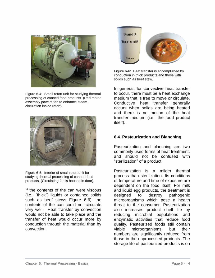
Chapter 6: Thermal Processing - Basics Page 6 - 4
Figure 6-4: Small retort unit for studying thermal processing of canned food products. (Red motor assembly powers fan to enhance steam circulation inside retort).
Figure 6-5: Interior of small retort unit for studying thermal processing of canned food products. (Circulating fan is housed in door).
If the contents of the can were viscous (i.e., “thick”) liquids or contained solids such as beef stews Figure 6-6), the contents of the can could not circulate very well. Heat transfer by convection would not be able to take place and the transfer of heat would occur more by conduction through the material than by convection.
Figure 6-6: Heat transfer is accomplished by conduction in thick products and those with solids such as beef stew. In general, for convective heat transfer to occur, there must be a heat exchange medium that is free to move or circulate. Conductive heat transfer generally occurs when solids are being heated and there is no motion of the heat transfer medium (i.e., the food product itself). 6.4 Pasteurization and Blanching Pasteurization and blanching are two commonly used forms of heat treatment, and should not be confused with “sterilization” of a product. Pasteurization is a milder thermal process than sterilization. Its conditions of temperature and time of exposure are dependent on the food itself. For milk and liquid egg products, the treatment is designed to destroy pathogenic microorganisms which pose a health threat to the consumer. Pasteurization also increases product shelf life by reducing microbial populations and enzymatic activities that reduce food quality. Pasteurized foods still contain viable microorganisms, but their numbers are significantly reduced from those in the unprocessed products. The storage life of pasteurized products is on

Chapter 6: Thermal Processing - Basics Page 6 - 5
the order of several weeks under refrigerated conditions. Pasteurization is most frequently applied to liquid products such as milk, liquid egg products, wines, beers, fruit juices, and perhaps yoghurts (with no live cultures). Blanching might best be described as the equivalent of pasteurization for fruits and vegetables. Its primary aim is to deactivate enzymes present in the foodstuff that would cause quality degradation, even under refrigerated or frozen storage conditions. Some microorganisms will be destroyed during the blanching process. Fruits or vegetables that are to be canned, rather than frozen, would need to be heat treated to a commercially sterile level, rather than being blanched. Consider the following example, which has been discussed previously in Chapter 2. If not properly blanched, cauliflower will turn brown or almost black in colour during frozen storage, and its quality will suffer (Figure 6-7). If, on the other hand, blanching conditions are too severe, the product quality will suffer from the excessive thermal treatment. The enzyme responsible for this browning is polyphenol oxidase. It is inactivated when subjected to high temperatures and loses its ability to catalyze the degradation reactions that lead to the development of the objectionable dark colouration in the cauliflower.
Figure 6-7: Unblanched cauliflower will turn brown due to the degradative action of polyphenol oxidase.
Many vegetables (e.g., carrots, turnip, parsnips, potatoes, and radishes, etc.) contain an enzyme known as peroxidase. While peroxidase does not lead to any degradation, it can be used as an indicator enzyme. During their normal growth, plant tissues produce small amounts of peroxide as by-products of their metabolism. If peroxide was allowed to accumulate, its concentration could reach levels that were harmful to the plant. Having peroxidase present catalyzes the decomposition of any peroxide present into water and oxygen, which are harmless. The reaction sequence is shown in Figure 6-8.
Figure 6-8: Reaction catalyzed by peroxidase.
Since oxygen is a gas, it will be given off as indicated by the vertical arrow in the reaction. We can examine how blanching works by using the peroxidase enzyme catayzed reaction. The important thing to recognize is that peroxidase is less sensitive to heat than many of the enzymes that degrade the product. Unlike enzymes such as polyphenol

Chapter 6: Thermal Processing - Basics Page 6 - 6
oxidase, peroxidase is very easy to detect, which is why it is used as an indicator enzyme. If there is no peroxidase present after blanching, the other less heat-resistant enzymes will have also been deactivated. In Figure 6-9, we see fresh radishes which naturally contain the peroxidase enzyme.
Figure 6-9: Fresh radishes prior to blanching.
The presence of peroxidase can be verified by pouring a weak peroxide solution over thin slices of freshly cut radish. A 3% peroxide solution similar to that used for home first-aid purposes is sufficient for this convenient test. Figure 6-10 shows how peroxidase in the radish slices acts on the peroxide solution and creates small bubbles of oxygen. Similar observations were made when using slices of turnip, carrot, parnsnips, and potatoes.
Figure 6-10: Sliced unblanched radishes in hydrogen peroxide solution (note the oxygen bubbles).
A second set of radish slices was then blanched by placing them in boling water for approximately three minutes (Figure 6-11). The blanched slices were then plunged into cold water to halt the heating process.
Figure 6-11: Radish slices were blanched in hot water for 3 minutes.
Heating deactivates the peroxidase enzyme and prevents the decomposition of peroxide from taking place. Figure 6-12 shows how no reaction products can be formed if the enzyme has become inactive.
Figure 6-12: Inactivation of the peroxidase stops the reaction.

Chapter 6: Thermal Processing - Basics Page 6 - 7
To verify the success of the blanching, we can pour the weak peroxide solution over slices of the blanched radish. If there is no enzyme activity present, no oxygen bubbles should be observed, which is the case here. This is confirmed in Figure 6-13.
Figure 6-13: Sliced blanched radishes in hydrogen peroxide solution (note the absence of any oxygen bubbles).
Similar sets of results were obtained in tests with other vegetables. Figure 6-14 shows raw turnip slices in a solution of hydrogen peroxide. The small oxygen bubbles around the slices indicate the presence of the peroxidase enzyme.
Figure 6-14: Unblanched turnip slices in a hydrogen peroxide solution.
After blanching for several minutes in boiling water, the test for the peroxidase enzyme was repeated. As can be seen
in Figure 6-15, there are no oxygen gas bubbles present around the turnip slices. This indicates that the peroxidase has been inactivated by the heat treatment step, as was observed previously in the case of the radishes.
Figure 6-15: Slices of blanched turnip in a hydrogen peroxide solution. Note the absence of oxygen bubbles.

Chapter 6: Thermal Processing - Basics Page 6 - 8
6.5 Pasteurization and the Thermal Processing of Milk The topic of “pasteurization” is really a sub-topic of product sterilization and thermal processing. Its commercial importance, particularly in the processing of dairy products makes it worthy of individual coverage. The times and temperatures given here should be considered as guidelines. Actual processing conditions are stipulated by laws within the jurisdictions in which the milk is processed. These conditions must be met in order to offer milk for commercial sale. Sources of information pertaining to processing conditions are normally available from the regulatory agencies responsible for milk processing in a particular country, state, or province. Pasteurization has “evolved” over the years from simple batch heating in an open kettle or vat to the more sophisticated continuous processes in use today. In all cases, the objectives are the same - to destroy spoilage organisms, pathogenic organisms, and degradative enzymes, in order to enhance quality, safety, and storage life. Batch pasteurization of milk was one of the earliest thermal processes for liquid food products. In early pasteurization processes, the milk was placed in a jacketed kettle and heated to 62°C (143°F) and held for 30 minutes. After being cooled, the milk was packaged. The original batch pasteurization process for milk was designed to ensure the destruction of Mycobacterium tuberculosis. This is a highly-heat resistant non-spore-forming bacterium that is capable of transmitting
tuberculosis to humans. The heat treatment required for this process was 62°C (143°F) for 30 minutes. Later Coxiella burnetii, the microorganism responsible for causing Q fever, was discovered in milk. It required a temperature of 63°C (145°F) for 30 minutes to ensure its destruction (Potter& Hotchkiss, 1995). While 30 minutes of exposure to a temperature of 63°C was sufficient to destroy the undesirable microorganisms present in the milk, it also destroyed the milk’s flavour. Long holding times also made it impractical to process milk on a continuous basis. In continuous processing, the product is heated to the desired temperature and pumped through a length of stainless steel pipe or tubing. The combination of the length of the tubing, its diameter, and its flowrate, determine how long the product stays in this “holding tube”. Shorter holding times were needed from both a quality and processing point of view. Through investigation of relationships between temperature and time, it was found that even a modest increase in temperature was sufficient to significantly reduce the required processing time. By increasing the temperature of the milk to 71.5°C (approximately 161°F), the holding time could be reduced to 15 seconds. The temperature is frequently rounded upwards to 72°C (approximately 162°F), or even slightly higher (Potter & Hotchkiss, 1995). This was ideally suited for continuous processing and is often referred to as “high temperature - short time” or HTST processing. The equipment used in HTST processing is discussed later in this section. Actual

Chapter 6: Thermal Processing - Basics Page 6 - 9
times and temperatures vary for each individual liquid product and also depend on the microbial load present. Although milk is the most commonly pasteurized food product, liquid egg is also pasteurized. Liquid whole eggs or egg whites can be pasteurized at 60°C to 62°C (approximately 140°F to 144°F) for 3.5 to 4.0 minutes. Such processing is designed to reduce the risk of salmonella. However, when using liquid egg products (or even fresh shell eggs), it is necessary to ensure that they are adequately cooked. Listeria is also becoming a concern in egg products (Potter & Hotchkiss, 1995). Fruit juice-based beverages may also be thermally processed for packaging in what is generically known as aseptic packages or “drink boxes”. This technology, pioneered by Tetra Pak of Lund, Sweden, brings together sterile packing material with thermally processed beverages and forms the package around the beverage in a sophisticated packaging machine (Figure 6-16). Typically, the liquid beverage is heated to temperatures in excess of 90°C (194°F) and held for 20 to 30 seconds. Actual times and temperatures depend on the product and a number of other factors.
Figure 6-16: Schematic representation of an aseptic process.
A more recent development in milk pasteurization has been the development of an “ultra-high temperature” or UHT thermal process for milk. It uses temperatures as high 150°C (302°F) and holding times as low as 2 seconds for acidic juices. This achieves an extremely high degree of destruction of any microorganisms that are present (Potter and Hotchkiss, 1995). Processing conditions for milk in Canada are presented in Table 6-1.
Table 6-1: Time and Temperature Relationships for Milk Pasteurization by Various Methods (Canadian Dairy
Information Centre and CFIA)
Batch Processing 30 minutes at 63°C
High Temperature Short Time (HTST) 15 seconds at 72°C (often 30 seconds)
Ultra High Temperature (UHT) 140°C for 5 seconds (minimum)

Chapter 6: Thermal Processing - Basics Page 6 - 10
Special equipment is essential for UHT processing and frequently involves injection of high pressure steam directly into the liquid product. The condensed steam may dilute the product somewhat, but this excess water may be removed by “flashing” it off after the time at temperature has been achieved. Heating processes based on “steam injection” (Figure 6-17) and “steam infusion” (Figure 6-18), can be used in these applications.
Figure 6-17: Steam injection system for heating liquid products.
Figure 6-18: Steam infusion system for heating liquid products.
In both the HTST and UHT processes, the temperature of the milk can be raised very rapidly from its initial refrigerated temperature of 4°C (approximately 39°F) to the desired processing temperature. Once it is held at that temperature for the specified period of time, the temperature of the milk can be rapidly lowered so that it is suitable for packaging. This is in contrast to the long time periods necessary to raise the temperature of milk in an old-fashioned batch kettle operation and to bring its temperature back down once it had been sufficiently heat treated.

Chapter 6: Thermal Processing - Basics Page 6 - 11
6.5.1 Indicator Enzymes in Milk Pasteurization In order to determine if milk has been effectively pasteurized, alkaline phosphatase is used as an indicator. It is an enzyme that is naturally found in milk This enzyme responds to time-temperature exposure in a manner very similar to the microorganisms present in milk. If the milk undergoes sufficient heating (i.e., greater than 72°C) for the prescribed period of time (i.e., greater than 15 seconds), then the alkaline phosphatase present in the milk will be deactivated. Alkaline phosphatase can then be used to monitor the degree of pasteurization that a particular processing run of milk has had. If the residual enzyme concentration is above a specified value, the degree of pasteurization has been insufficient to meet processing requirements (Potter & Hotchkiss, 1995). In testing for alkaline phosphatase activity, a colorimetric method is employed. The enzyme catalyses the breakdown of phenolphosphoric acid which yields phenol as one of its reaction products. The free phenol can react with organic compounds to give a blue colour. In one test for alkaline phosphatase, disodium phenol phosphate is added to a milk sample as a source of phenol and the mixture is incubated. An indicator reagent, 2,6,dichloroquinonechloride is then added. Should a blue colour develop, then the milk is considered to be inappropriately pasteurized. The enzyme test has posed some problems to processors who wish to filter their milk rather than heat process
it. Many jurisdictions still require a minimal heat process to inactivate the indicator enzyme in order to be certain that the milk has been adequately processed. One argument for maintaining the heat treatment as a legal requirement to offer the milk for sale is that there are no guarantees that the filtration system has not developed small pinholes that would allow contaminating microorganisms to pass through. The combination of filtration and minimal heat treatment addresses this issue while producing a high quality, safe product.

Chapter 6: Thermal Processing - Basics Page 6 - 12
6.6 Batch and Continuous Thermal Processes As previously stated, thermal processing for the destruction of microorganisms is highly dependent on both time and temperature. The higher the temperature, the shorter the holding time that is required to obtain the desired “degree of kill”. Conversely, lower temperatures require significantly longer periods of time for an equivalent “degree of kill”. There are two basic approaches to thermally processing food products. They are based on batch or continuous methods. Many batch processes are routinely done in large “kettles” or other suitable vessels. As seen in Figure 6-19, heat is applied to warm the product to the desired final temperature (time = t0 to t1). Once at that temperature, the product is held there for a prescribed length of time (time = t1 to t2), and is then cooled (time = t2 to t3). Depending on the heating method and rate of heat addition, the product can take a range of times to reach its holding temperature.
Figure 6-19: The temperature rises and falls slowly in most batch processes.
There are other factors which influence the time-to-temperature in a batch process as well; including:
• size of the vessel being heated • degree of insulation of the vessel • amount of surface area available for
heat transfer • method of heat application (direct or
indirect) • temperature differential between the
product and heating medium • nature of the product itself • temperature of the surroundings
(plus air flow) • agitation vs non-agitation • etc.
Similar factors influence the time for cooling the product after its holding time. The holding time in a batch process is difficult to control in an exact manner. Essentially, there is a reliance on having a minimum holding time, which then tends to “over-process” the product as the cooling sequence is started. Continuous processes use various types of heat exchangers to heat and cool product. Holding times are achieved through the use of holding tubes positioned between the heating and cooling stages of the process. Pumps move the product through the system. Figure 6-20 shows a relative representation of times required to bring the product up to temperature (time = t0 to t1) and to cool it (time = t2 to t3). These times are generally much shorter than for a batch process with similar temperature requirements. The holding time (time = t1 to t2) is also much more controlled.

Chapter 6: Thermal Processing - Basics Page 6 - 13
Figure 6-20: Diagram showing the more rapid temperature changes occurring in a continuous thermal process.
In comparing the various times in Figures 6-19 and 6-20, it is important to note that the holding times are equal since the heat treatment process dictates a specific time at a prescribed temperature. It is the time taken to reach the desired holding temperature and the cooling time that are the major concerns. In Figures 6-19 and 6-20 there are three distinct regions where there will be some degree of microbial destruction due to the time at an elevated temperature. These three regions correspond to the heating, holding, and cooling portions of the curves. From this, it follows that there are three “sterilization” portions in the process, each contributing to the overall sterilization (Holdsworth, 1997). In the batch process (Figure 6-19), contributions from the heating and cooling stages of the heat treatment process can be quite significant. In a continuous process (Figure 6-20) where the time-to-temperature is a more rapid change, the effects on the
sterilization process are relatively minor. This is also true of the reasonably rapid change for cooling. Here, a processor would be tempted to consider only the actual time-at-temperature as doing the “pasteurization”, while the time up and time down would act as a small insurance policy in assuring that there was sufficient time to carry out the desired degree of kill. In all cases, when designing a thermal process to treat a food product, experimental or empirical data are preferred to theoretical calculations. In an ideal system, the temperature would rise to the desired level instantaneously by what is referred to as a “step change”. After the required time at temperature, the temperature could be brought down to a much lower level in a second step change. While this is not actually possible, modern heat exchange equipment can significantly reduce the time to raise and lower the temperature of food products so that they are very short. Figure 6-21 shows this diagrammatically.
Figure 6-21: Diagram of step changes in temperature in a thermal process.
The design of a thermal process and selection of the appropriate equipment is complex. To ensure all thermal

Chapter 6: Thermal Processing - Basics Page 6 - 14
criteria and legislative requirements are being met, you should work with a reputable supplier having experience in this area. 6.6.1 Effects of Particle Size on Heat-up Time of Solids When particles are present in products that are being heat treated, it is necessary to consider the time it takes for heat to penetrate to the centre of the particle. Characteristic dimensions are used to describe the two shapes of particles that are generally found in food products. These dimensions account for the heat penetration to the centre of the particles. For a spherical particle, the characteristic dimension would be its diameter, or possibly its radius, which is simply one half of the diameter. For flat particles, the characteristic dimension would be its thickness, or perhaps its half-thickness since this is the distance that the heat must penetrate to reach the centre from each side. For very thin flat material such as pulp in orange juice, the particles are so thin that there is an almost negligible time for the heat to penetrate to their centre. Figure 6-22 shows orange pulp that has been removed from orange juice and washed prior to be re-suspended in fresh water.
Figure 6-22: Washed pulp from orange juice resuspended in fresh water. Note its thinness.
As can be seen, the orange juice pulp is very thin and will offer little or no resistance to heat penetration. However, in stews or beans in tomato sauce (Figure 6-23) which contain larger pieces of solids, the time it takes for heat to reach their centres can be quite appreciable.
Figure 6-23: Beans in tomato sauce will take an appreciable time to heat in the can due to the size of the “particles” (i.e., the beans).
Due to the effects of size on the time it takes for particles to reach the target processing temperatures, it is often necessary to avoid processing products with large particle sizes in continuous thermal processes. Alternately, it may be possible to make modifications to a process to accommodate the need for longer holding times. In some cases, extremely long hold tubes with large

Chapter 6: Thermal Processing - Basics Page 6 - 15
diameters are used to achieve holding times of several minutes. As an alternative, stews may be placed in cans which are then sealed and placed in large retorts where they are subjected to heat treatment. Table 6-2 summarizes the approximate times taken for particles of various sizes to reach 99% of their final target temperature in a thermal process.
Table 6-2: Approximate Times Taken for Particles of Various Sizes to Reach 99% of Final Temperature
Particle Size (Diameter or Thickness)
Time to Reach 99% of Final Temperature
1.0 x 10⁻⁴ cm 1 microsecond
1.0 x 10⁻³ cm 0.1 millisecond
1.0 x 10⁻² cm 10 milliseconds
1.0 x 10⁻¹ cm 1.0 second
1.0 cm 100 seconds
Source unknown
6.7 Equipment Used in Heating and Cooling The following diagrams illustrate various pieces of equipment used in thermal processing (and cooling) of liquid food products. They include:
• Jacketed Kettles • Plate Heat Exchangers • Tubular Heat Exchangers • Scraped Surface Heat Exchangers • Shell and Tube Heat Exchangers
Only brief descriptions of how they operate are provided below. For more details, you may wish to consult Internet sources, or contact a reputable equipment supplier. 6.7.1 Jacketed Kettles One of the simplest and most commonly used methods of heating (or cooling) liquid products in food production facilities is the jacketed kettle or tank. Product is introduced into the vessel and steam or hot water is circulated through the outer jacket of the tank to heat its contents. Figure 6-24 shows a jacketed kettle in a pilot-plant facility.
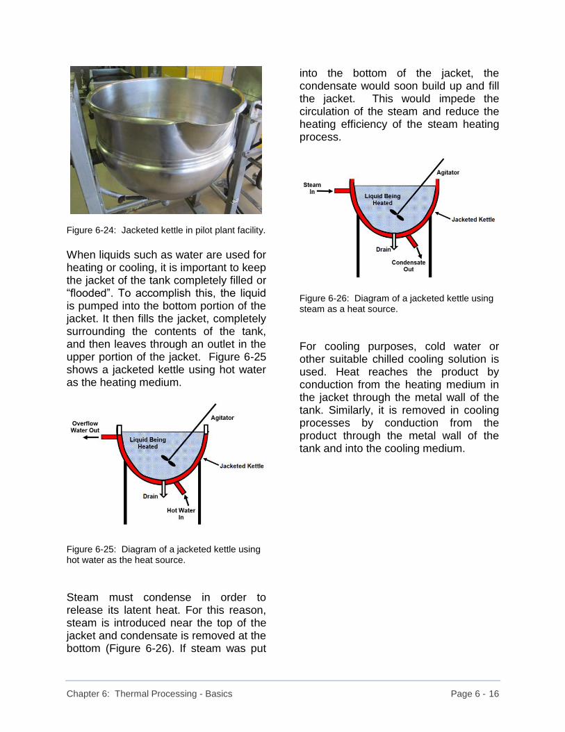
Chapter 6: Thermal Processing - Basics Page 6 - 16
Figure 6-24: Jacketed kettle in pilot plant facility.
When liquids such as water are used for heating or cooling, it is important to keep the jacket of the tank completely filled or “flooded”. To accomplish this, the liquid is pumped into the bottom portion of the jacket. It then fills the jacket, completely surrounding the contents of the tank, and then leaves through an outlet in the upper portion of the jacket. Figure 6-25 shows a jacketed kettle using hot water as the heating medium.
Figure 6-25: Diagram of a jacketed kettle using hot water as the heat source.
Steam must condense in order to release its latent heat. For this reason, steam is introduced near the top of the jacket and condensate is removed at the bottom (Figure 6-26). If steam was put
into the bottom of the jacket, the condensate would soon build up and fill the jacket. This would impede the circulation of the steam and reduce the heating efficiency of the steam heating process.
Figure 6-26: Diagram of a jacketed kettle using steam as a heat source.
For cooling purposes, cold water or other suitable chilled cooling solution is used. Heat reaches the product by conduction from the heating medium in the jacket through the metal wall of the tank. Similarly, it is removed in cooling processes by conduction from the product through the metal wall of the tank and into the cooling medium.

Chapter 6: Thermal Processing - Basics Page 6 - 17
6.7.2 Plate Heat Exchangers Plate heat exchangers are the true workhorse of most processes for heat treating liquids such as milk or juice-based beverages. One of the main factors in determining how rapidly a liquid reaches its target processing temperature is the distance that the heat must travel through the liquid. Plate heat exchangers create a thin layer or channel of liquid between two parallel stainless steel plates. If there is steam or hot water on the opposite side of these plates, then heat will be transferred rapidly to the liquid and it will soon reach its desired temperature. A similar approach can be used for cooling. Figure 6-27 shows a schematic representation of a series of plates with liquid product and heating medium flowing between them in the appropriate manner.
Figure 6-27: Heat from hot water is transferred through metal plates to warm cold product in a plate heat exchanger.
In thermal processes, it is imperative that the product not only be heated to the prescribed final temperature, but it also must be held there for a specified period of time. This is accomplished by means of a holding tube which has been discussed previously. Once held for the appropriate length of time, the product must be cooled rapidly to avoid risking heat damage. A plate heat exchanger may also be used for this purpose along with chilled water or other suitable cooling medium. In examining the overall process, it can be seen that there is an appreciable amount of heat that must be added to the liquid product in the heating stage, and a substantial amount of heat that also must be removed in the cooling stage. In the interest of energy conservation, it would be ideal if the heat that must be removed from the heat-treated product could be used to warm the incoming unprocessed liquid. This is actually what happens in the heat “regeneration” section of a heat exchanger system. Such a heat exchanger system typically consists of three sections - a heating section, a cooling section, and a regeneration or “regen” section. Figure 6-28 shows this arrangement.
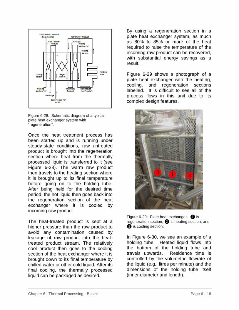
Chapter 6: Thermal Processing - Basics Page 6 - 18
Figure 6-28: Schematic diagram of a typical plate heat exchanger system with “regeneration”.
Once the heat treatment process has been started up and is running under steady-state conditions, raw untreated product is brought into the regeneration section where heat from the thermally processed liquid is transferred to it (see Figure 6-28). The warm raw product then travels to the heating section where it is brought up to its final temperature before going on to the holding tube. After being held for the desired time period, the hot liquid then goes back into the regeneration section of the heat exchanger where it is cooled by incoming raw product. The heat-treated product is kept at a higher pressure than the raw product to avoid any contamination caused by leakage of raw product into the heat-treated product stream. The relatively cool product then goes to the cooling section of the heat exchanger where it is brought down to its final temperature by chilled water or other cold liquid. After its final cooling, the thermally processed liquid can be packaged as desired.
By using a regeneration section in a plate heat exchanger system, as much as 80% to 85% or more of the heat required to raise the temperature of the incoming raw product can be recovered, with substantial energy savings as a result. Figure 6-29 shows a photograph of a plate heat exchanger with the heating, cooling, and regeneration sections labelled. It is difficult to see all of the process flows in this unit due to its complex design features.
Figure 6-29: Plate heat exchanger. ❶ is
regeneration section, ❷ is heating section, and
❸ is cooling section.
In Figure 6-30, we see an example of a holding tube. Heated liquid flows into the bottom of the holding tube and travels upwards. Residence time is controlled by the volumetric flowrate of the liquid (e.g., litres per minute) and the dimensions of the holding tube itself (inner diameter and length).

Chapter 6: Thermal Processing - Basics Page 6 - 19
Figure 6-30: Holding tube section of heat exchanger system. Arrows indicate direction of fluid flow.
The slope of the holding tube is usually specified by government agencies responsible for food processing. In order to reduce heat loss, holding tubes are most often covered with a layer of insulation. No such insulation is in place on the holding tube in the photo above. It is also important to recognize that the residence time distribution pattern of liquid in the holding tube may not be uniform. Liquid travelling down the centre of the holding tube may actually be moving faster than the average linear velocity of the liquid (e.g. measured in metres per second or centimetres per second). This is due to the liquid near the interior walls of the holding tube experiencing “drag”, where its forward velocity is slowed appreciably. Let’s consider a very small particle suspended in the liquid, or a small volume of liquid that we will call a “volume element”. The fastest moving
particles moving down the centre of the holding tube will not experience the same holding time as the particles or volume elements of liquid travelling at the average velocity. In order to account for these fastest moving particles and ensure that they are receiving the required time at the specified temperature, the holding tube is often lengthened. While this may over-process some of the liquid to a certain degree, the risk of having under-processed product is minimized. Sizing of the holding tube and other details of the design of a plate heat exchanger system are best handled by a knowledgeable and reliable equipment supplier. In all thermal processing systems, it is imperative that the time-temperature relationship meet regulatory standards. Having met the residence time requirements by means of the holding tube dimensions and flowrate of the product, it is now essential to monitor the temperature of the liquid as it leaves the holding tube. If the temperature falls below the required temperature, the thermal process is no longer in compliance with government regulations. To avoid this liquid going any further in the process, a temperature sensor is installed at the end of the holding tube. In the event that the temperature falls below a pre-set value, the temperature sensor will trigger a flow diversion valve that will automatically re-direct the insufficiently heated product back to the start of the thermal process. Flow will not be restored to the downstream part of the process until such time as the temperature is restored to its required level.

Chapter 6: Thermal Processing - Basics Page 6 - 20
A flow diversion valve is shown in Figure 6-31. Heated liquid leaving the cooling section of the heat exchanger enters the flow diversion valve assembly as indicated by . If the temperature leaving the holding tube and entering the regeneration section was above the required value (e.g., 72°C for milk pasteurization), the flow will be directed to the packaging line or sterile storage tank in preparation for packaging (i.e., ). If the temperature is below the regulated value, the flow diversion valve will send the improperly processed cool product back to the start of the process (i.e., ). Usually, this means the cool improperly processed liquid will go back to the balance tank from where it will proceed through the process again. Once the required temperature at the end of the holding tube has been re-established (i.e., above 72°C for milk) the flow diversion valve will re-direct the liquid to the downstream packaging or storage system once again. The direction in which the flow diversion valve sends the product is controlled by a piston (i.e., ) which is raised or lowered by an air-activated solenoid unit (i.e., ). The solenoid unit acts on a signal received from the temperature sensor at the end of the holding tubes. Figure 6-32 shows how the diversion valve is positioned after the final product cooling section. It receives a signal from the temperature sensor at the end of the holding tube indicating whether to allow the flow to continue in its normal flow direction to the packaging area, or to divert the flow back to the balance tank at the start of the thermal process.
Figure 6-31: Flow diversion valve (numbered items are explained in text).
Figure 6-32: Schematic diagram of flow diversion valve position.
In many countries or states, regulations declare that a chart must be in place to record the temperature at the end of the holding tube during the times that the process is in operation. Often, it is stipulated that the chart must be circular and record twelve hours of operation per rotation. Charts must be changed every twelve hours and be properly labelled with dates and other relevant production data. A circular chart is shown in Figure 6-33.

Chapter 6: Thermal Processing - Basics Page 6 - 21
Figure 6-33: Circular recording chart for a thermal processing unit.
6.7.3 Tubular Heat Exchangers Tubular heat exchangers operate in a manner similar to jacketed tanks or kettles, but are generally used in continuous processes to continuously heat or cool liquid. Liquid product is pumped through a pipe or tube that is positioned inside a second section of tubing with a larger internal diameter. Hot water or steam is circulated through the outer section of tubing which forms a jacket around the inner length of tubing or pipe. Heat is then transferred through the wall of the inner section of pipe to the product. Cooling is accomplished in a similar manner using a chilled medium instead of hot water or steam. Figure 6-34 shows an end view of a tubular heat exchanger using hot water as the heat source. As can be seen from the side view in Figure 6-35, when hot water is used, it must flow into the lower portion of the shell and out through the upper portion to keep the shell “flooded” for efficient heat transfer. When steam is used as the heat source (Figure 6-36), it must be introduced at the top of the “shell” so that condensate can be drained from the shell. Tubular heat exchangers are more suitable for viscous products than are plate heat exchangers. Heating of viscous products between the plates of a plate heat exchanger may result in product scalding or burning onto the hot metal surfaces and plugging the plate heat exchanger.

Chapter 6: Thermal Processing - Basics Page 6 - 22
Figure 6-34: Tubular heat exchanger (end view) showing use of hot water to warm the product.
Figure 6-35: Tubular heat exchanger using hot water as a source of heat.
Figure 6-36: Tubular heat exchanger using steam as a source of heat.
6.7.4 Scraped Surface Heat Exchangers Scraped surface heat exchangers are basically tubular heat exchangers that have been modified to accommodate viscous products and overcome problems of burn-on or product scalding. When viscous liquids like ice cream premixes pass through a heat exchanger, they do not flow as easily as milk or juice-based beverages. They are thick and tend to stick to hot surfaces when heated. In order to prevent the material from burning onto the hot metal surface of the heat exchanger, scraper blades can be incorporated into the heat exchanger design (see Figure 6-37). The blades are powered by a motor assembly at the end of the heat exchanger. As they rotate, they scrape the viscous material away from the hot metal walls and allow cooler material to flow in behind them. This mixing is similar to that used when preparing milk puddings on a stove-top when constant stirring is required to prevent the pudding from burning onto the bottom of the pot or developing an overheated scalded flavor. Scraped surface heat exchangers are also used to cool viscous product. Here, the scraper blades prevent product from freezing onto the cold metal surface of the heat exchanger. An added feature in the manufacture of ice cream is the aeration of the cooled mixture with air sparged into the heat exchanger through a system mounted within the central shaft of the cooling unit. This device is called a “dasher”.

Chapter 6: Thermal Processing - Basics Page 6 - 23
Figure 6-37: Scraped surface heat exchanger.
6.7.5 Shell and Tube Heat
Exchangers Shell and tube heat exchangers (see Figure 6-38) consist of a number of small diameter tubes arranged in a bundle inside a larger section of pipe or tubing. They are a further modification of the basic tubular heat exchangers discussed previously. Product flows into a manifold at the feed end of the shell and tube heat exchanger where it is forced to spread out and travel through the smaller tubes. These small diameter tubes provide a large surface area for heat exchange with the heating or cooling medium passing through the outer shell of the unit. At the end of the shell and tube heat exchanger the small tubes empty into a second manifold which then allows the liquid to come together and enter a single discharge pipe or tube and leave the heat exchanger.
Figure 6-38: End view of a shell and tube heat exchanger using hot water as the heat source.
Figure 6-39 shows a side view of the shell and tube heat exchanger with hot water being used as the heat source. To keep the shell flooded, hot water is introduced from the bottom and leaves from the top.
Figure 6-39: Side view of shell and tube heat exchange with hot water as the heat source.
When steam is used as the heat source, it is necessary to introduce the steam through an inlet in the top of the shell and then drain the condensate out the bottom (Figure 6-40). Failure to do so will fill the shell with condensate and reduce the heating efficiency since heat is liberated through the condensation of steam in the shell.
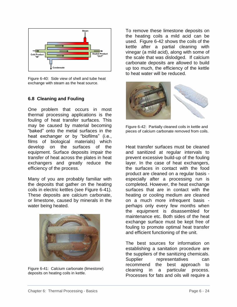
Chapter 6: Thermal Processing - Basics Page 6 - 24
Figure 6-40: Side view of shell and tube heat exchange with steam as the heat source.
6.8 Cleaning and Fouling One problem that occurs in most thermal processing applications is the fouling of heat transfer surfaces. This may be caused by material becoming “baked” onto the metal surfaces in the heat exchanger or by “biofilms” (i.e., films of biological materials) which develop on the surfaces of the equipment. Surface deposits impair the transfer of heat across the plates in heat exchangers and greatly reduce the efficiency of the process. Many of you are probably familiar with the deposits that gather on the heating coils in electric kettles (see Figure 6-41). These deposits are calcium carbonate, or limestone, caused by minerals in the water being heated.
Figure 6-41: Calcium carbonate (limestone) deposits on heating coils in kettle.
To remove these limestone deposits on the heating coils a mild acid can be used. Figure 6-42 shows the coils of the kettle after a partial cleaning with vinegar (a mild acid), along with some of the scale that was dislodged. If calcium carbonate deposits are allowed to build up too much, the efficiency of the kettle to heat water will be reduced.
Figure 6-42: Partially cleaned coils in kettle and pieces of calcium carbonate removed from coils.
Heat transfer surfaces must be cleaned and sanitized at regular intervals to prevent excessive build-up of the fouling layer. In the case of heat exchangers, the surfaces in contact with the food product are cleaned on a regular basis - especially after a processing run is completed. However, the heat exchange surfaces that are in contact with the heating or cooling medium are cleaned on a much more infrequent basis - perhaps only every few months when the equipment is disassembled for maintenance etc. Both sides of the heat exchange surface must be kept free of fouling to promote optimal heat transfer and efficient functioning of the unit. The best sources for information on establishing a sanitation procedure are the suppliers of the sanitizing chemicals. Supplier representatives can recommend the best approach to cleaning in a particular process. Processes for fats and oils will require a

Chapter 6: Thermal Processing - Basics Page 6 - 25
different cleaning procedure than for a process involving proteins or carbohydrates. What works in one cleaning application may not work in another application. A typical cleaning process in a juice process may involve the use of a caustic wash followed by a water rinse, followed by an acid wash, and a second water rinse. The actual temperatures and concentrations of cleaning solutions depend on the particular cleaning agents being used. Often, a chlorine rinse or specialty detergents may also be involved. In cleaning a continuous process, a “clean-in-place” (CIP) procedure is most frequently used. Sanitizing chemicals are prepared in large tanks that serve as reservoirs from which they can be withdrawn. These chemical solutions are pumped as required through the process after a production run has been completed. Such procedures are frequently computer controlled. During the CIP procedures, flow rates are used that may be much higher than those used during processing. Such high flow rates maintain a high level of turbulence in the equipment, thereby ensuring that all contact surfaces are exposed to the sanitizing agents. For cleaning tanks and other large enclosed vessels, spray balls or oscillating spray nozzle assemblies are used to direct the cleaning solutions to all surfaces of the vessel.
6.9 Summary Comments Now that we have discussed some of the basic concepts of thermal processing and examined various types of equipment, we can move on to look at thermal processing calculations. This is done in the following chapter. 6.10 References Government of Canada, Canadian Dairy Information Centre. Available on-line at: www.dairyinfo.gc.ca/index_e.php?s1=dr-rl&s2=canada&s3=ndc-cnpl&s4=05-2005 See Schedule 1 (accessed March 2018). Government of Canada, Canadian Food Inspection Agency (CFIA). “Milk and Regulated Milk Products – Import Procedures”. Available on-line at: www.inspection.gc.ca/animals/terrestrial-animals/imports/policies/animal-products-and-by-products/2001-4/eng/1321120021415/1321120121634 (accessed March 2018) Holdsworth, D.S. “Thermal Processing of Packaged Foods – First Edition”, Food Engineering Series, Springer, New York, 1997. Potter, Norman N. and Joseph H. Hotchkiss. “Food Science” (Second Edition). Chapman and Hall, New York, 1995.

Chapter 7: Thermal Processing – Specialized Calculations Page 7 - 1
7. Thermal Processing – Specialized Calculations 7.1 Introduction Chapter 7 deals with a number of specialized calculations pertaining to thermal processing. These calculations may only be required by individuals who are working with heat exchangers and larger scale operations. The information in this chapter is intended to explain how variations in temperature can affect processing times and to show how time-temperature relationships impact the degree of destruction of contaminating microorganisms. You will recall, in the previous chapter, we discussed the differences between batch and continuous thermal processes. One of the significant differences between these two approaches was the relatively long time required to heat the product to its desired temperature and cool it at the end of the holding period in the batch method. As a result, the “come-up” and come-down” times with batch processing contributed to the thermal destruction of the microorganisms in a rather significant manner. In contrast, the rapid “come-up” and “come-down” times commonly seen in continuous processing have little, if any, impact on the overall thermal process. They could essentially be ignored. For this reason, we will focus on calculations that apply more to continuous processing techniques than to batch processes.
7.2 Holding Times It should be emphasized that there are regulations in various jurisdictions that dictate how holding times are to be calculated. You must follow these regulations for the particular jurisdiction in which your product is to be sold. What follows in this chapter is a general overview of the topic. It is not meant to be used in place of local regulations and should not be construed as having any legal status. 7.2.1 Holding Time Calculations As product is pumped through the holding tube of a continuous thermal process, product along the walls of the pipe moves slower than product travelling down the centre of the pipe. This is due to viscous drag on the pipe walls. Therefore, there is a likelihood that the product is not being processed uniformly, or that each element of product is not seeing the same “thermal history” as the others. To recognize that the product moving down the centre of the pipe is not being heat treated for as long as the product at the walls, processors frequently hold the product for twice as long as the holding time calculated for the average moving particle. This allows for the fastest moving particles to move at twice the forward speed of the average moving particles and still be thermally processed for the minimum recommended time. However, this also means that a portion of the material will be processed for a somewhat longer

Chapter 7: Thermal Processing – Specialized Calculations Page 7 - 2
time period and may suffer some effects from prolonged exposure to the heat. The linear velocity of the average product particle can be calculated by dividing the volumetric flowrate of the product by the cross-sectional area of the holding tube (taking care to use dimensionally consistent units in the calculation). Average Velocity = volumetric flowrate . cross-sectional area = cm3 | = cm / sec. second | cm2 (Eq’n 7-1) To determine the length of hold tube required for the average moving particle, multiply the average velocity by the desired holding time. Tube length = Average Velocity x Holding Time = cm | sec = cm sec | (Eq’n 7-2) Once this length has been calculated, the actual holding tube can be made twice this length to accommodate the fastest moving particles. It is also possible to change the diameter of the holding tube rather than changing its length. If the inner diameter of the holding tube is doubled, the cross-sectional area of the tube will be increased by a factor of four. To double the volume of a given length of tubing, the inner diameter must be changed by
a factor of 1.41 (i.e., the square root of 2). In an existing hold tube, to find the average holding time, calculate the volume of the tube and divide it by the volumetric flowrate of the liquid travelling through it. Average holding time = Volume of Tube . Volumetric Flowrate = cm3 | second = seconds | cm3 (Eq’n 7-3) 7.2.2 Tests for Retention Time In some cases, it may not be sufficient to simply calculate the average retention time of a holding tube and double its length to account for the fastest moving fluid. You may need to have a more accurate picture of what is actually happening with regard to the residence time distribution of fluid in the holding tube. Hands-on tests can be conducted to determine holding times for existing equipment by such methods as: • injection of colored dyes • salt injection tests These methods will give a more precise determination of the actual holding times within a process. Ideally, a flat profile of liquid progressing through the hold tube is desired. In practice, there is generally a residence time distribution pattern that deviates from ideality.

Chapter 7: Thermal Processing – Specialized Calculations Page 7 - 3
Let’s take a look at how the two methods mentioned above can be used to determine the residence time distribution pattern or profile of liquid travelling through a holding tube. For the residence time test involving the injection of coloured dyes, it is necessary to have an inlet port in the holding tube very close to the start of the point at which it leaves the heating section of the heat exchanger. This is where the dye will be injected. It is also necessary to have a sampling port very close to the end of the holding tube just before it enters the regeneration section of the heat exchanger where the liquid product will be cooled. Figure 7-1 shows the locations of these ports.
Figure 7-1: Schematic diagram of set-up for dye injection test.
Once the process is operating under steady-state conditions, a concentrated dye can be injected through the inlet port at the exit from the heat exchanger. The colour of the dye should contrast as much as possible with the colour of the product. In tests with milk, we used a dark green dye with a strong tinctorial strength. In this way, the green colour was easily detected. At the same
instant as the dye is injected, a timer must be started. At regular intervals, small volume samples are withdrawn from the sampling port at the end of the holding tube and are placed in numbered containers such as test tubes. Initially, there will be no colour change to the product, since the dye will take some time to reach the sampling port. Dyed product moving along the centre of the holding tube will reach the sampling port first and there will be a slight tinge of colour to the product. As time goes on, the colour intensity will increase as the bulk of the dyed product reaches the sampling port. Once this product passes, the slowest moving product will reach the sampling port. The colour intensity will decrease until all of the dyed product has passed the sampling port and the product will return to its original colour. The numbered samples can then be tested for their colour intensity using a spectrophotometer or similar device. By plotting the colour intensity versus time, a residence time distribution pattern can be established. Figure 7-2 shows what a plot of colour intensity versus retention time could look like if the fastest and slowest moving particles in the liquid product were distributed equally on either side of the average retention time. This is a hypothetical example and is not based on actual data. Since this figure is intended to illustrate the concept of residence time distribution, no values are shown on the vertical and horizontal axes.
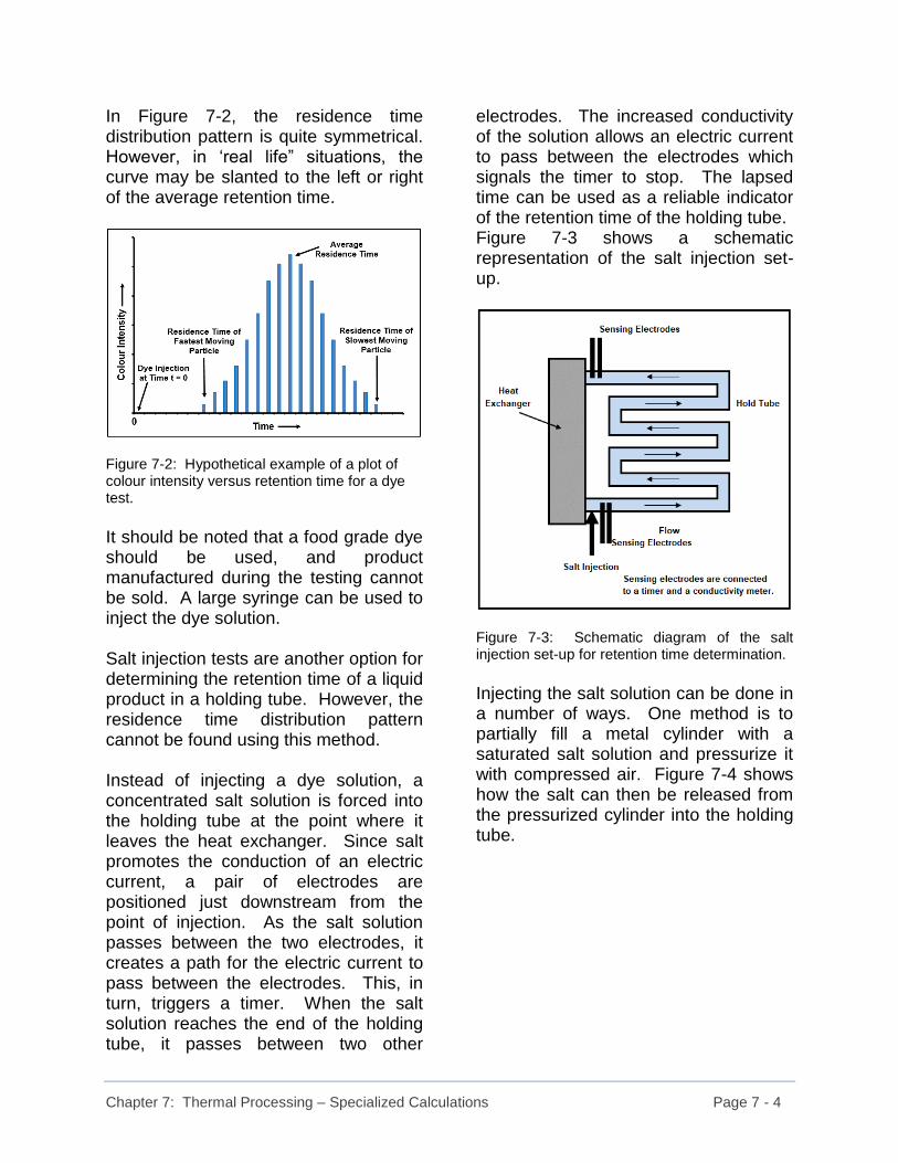
Chapter 7: Thermal Processing – Specialized Calculations Page 7 - 4
In Figure 7-2, the residence time distribution pattern is quite symmetrical. However, in ‘real life” situations, the curve may be slanted to the left or right of the average retention time.
Figure 7-2: Hypothetical example of a plot of colour intensity versus retention time for a dye test.
It should be noted that a food grade dye should be used, and product manufactured during the testing cannot be sold. A large syringe can be used to inject the dye solution. Salt injection tests are another option for determining the retention time of a liquid product in a holding tube. However, the residence time distribution pattern cannot be found using this method. Instead of injecting a dye solution, a concentrated salt solution is forced into the holding tube at the point where it leaves the heat exchanger. Since salt promotes the conduction of an electric current, a pair of electrodes are positioned just downstream from the point of injection. As the salt solution passes between the two electrodes, it creates a path for the electric current to pass between the electrodes. This, in turn, triggers a timer. When the salt solution reaches the end of the holding tube, it passes between two other
electrodes. The increased conductivity of the solution allows an electric current to pass between the electrodes which signals the timer to stop. The lapsed time can be used as a reliable indicator of the retention time of the holding tube. Figure 7-3 shows a schematic representation of the salt injection set-up.
Figure 7-3: Schematic diagram of the salt injection set-up for retention time determination.
Injecting the salt solution can be done in a number of ways. One method is to partially fill a metal cylinder with a saturated salt solution and pressurize it with compressed air. Figure 7-4 shows how the salt can then be released from the pressurized cylinder into the holding tube.
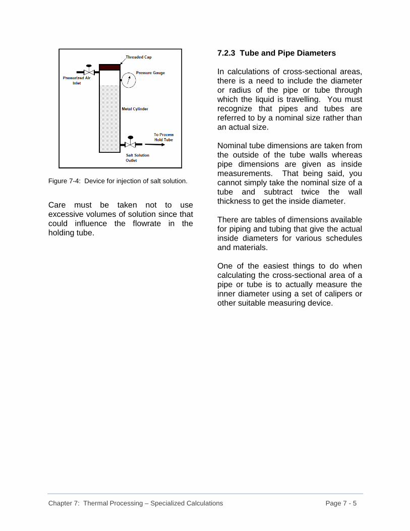
Chapter 7: Thermal Processing – Specialized Calculations Page 7 - 5
Figure 7-4: Device for injection of salt solution.
Care must be taken not to use excessive volumes of solution since that could influence the flowrate in the holding tube.
7.2.3 Tube and Pipe Diameters In calculations of cross-sectional areas, there is a need to include the diameter or radius of the pipe or tube through which the liquid is travelling. You must recognize that pipes and tubes are referred to by a nominal size rather than an actual size. Nominal tube dimensions are taken from the outside of the tube walls whereas pipe dimensions are given as inside measurements. That being said, you cannot simply take the nominal size of a tube and subtract twice the wall thickness to get the inside diameter. There are tables of dimensions available for piping and tubing that give the actual inside diameters for various schedules and materials. One of the easiest things to do when calculating the cross-sectional area of a pipe or tube is to actually measure the inner diameter using a set of calipers or other suitable measuring device.

Chapter 7: Thermal Processing – Specialized Calculations Page 7 - 6
7.2.4 Calculations involving Tube and Pipe Diameters A set of sample calculation will assist you in finding the cross-sectional area of a stainless steel tube and in finding the linear flow velocity for a given volumetric flowrate. This would be the type of calculation you would use for holding tubes in a thermal process. Let’s start with a 2.00 inch outer diameter stainless steel tube with a wall thickness of 0.049 inches. Even though most countries have adopted the metric system of measurement, many dimensions used in industry and various trades are still expressed in the “British” or “Sterling” system. Figure 7-5 shows a diagram of how the tubing dimensions are related.
Figure 7-5: Stainless steel tube dimensions.
Based on Figure 7-5, when we know the outer diameter and wall thickness, the inner diameter can be found by taking the outer diameter and subtracting twice the wall thickness. It is much easier to work with metric measurements in flowrate calculations than it is to work with “British” units. Therefore, it would be advantageous to work in centimeters rather than inches.
At this point, you have the choice of finding the inner diameter in inches and then converting it to centimeters, or converting both the outer diameter and wall thickness to centimeters before you calculate the inner diameter. Either way will work equally as well. However, finding the inner diameter in inches and then converting it to centimeters does save a conversion step. Inner = Outer – 2 x Wall diameter diameter thickness Outer diameter = 2.00 inches Wall thickness = 0.049 inches Inner diameter = 2.00” - 2 (0.049”) = 2.00” - 0.098” = 1.902” There are 2.54 cm in 1.0 inch Inner diameter = 1.902 inches x 2.54 cm inch = 4.83 cm Cross-sectional area = π r2 Since the diameter of a circle is equal to twice the radius, we can substitute “d/2” for the radius in this equation. Cross-sectional area = π r2 = π d2 4 π = 3.14159 Cross sectional area = 3.14159 | 4.83 cm | 4.83 cm . 4 | | = 18.32 cm2

Chapter 7: Thermal Processing – Specialized Calculations Page 7 - 7
Let’s suppose that the flowrate in the system is 5.0 litres per minute. We can now calculate the linear velocity in the tube. The key thing to remember is that 1 litre is equal to 1,000 mL and 1.0 mL is equal to 1 cm3. Dimensional analysis will help you keep the units straight and indicate to you whether you need to multiply or divide by the various values. Volumetric flowrate = 5.0 litres / minute = 5,000 mL / minute = 5,000 cm3 / minute From equation 7-1: Average linear velocity = Volumetric flowrate . Cross-sectional area = 5,000 cm3 | . minute | 18.32 cm2 = 272.93 cm / minute
≈ 273 cm / minute
If we want a 20 second average holding time in the tube, we can now calculate the length we would require. From equation 7-2: Tube Length = Average velocity x Holding Time = 273 cm | 20 sec. | minute . minute | | 60 sec. = 91 cm
Note how we had to include the conversion factor of 60 seconds per minute to make this equation behave correctly. This is because we have the average velocity in “cm / minute” and the holding time in “seconds”. These are not dimensionally consistent units, which meant we had to include the necessary conversion factor. If we wanted to be assured that the fastest moving particle going down the centre of the holding tube had a holding time of 20 seconds, we could double the length of the holding tube. This would make it 182 cm long instead of 91 cm long. Much of the product would then spend more than 20 seconds in the holding tube, but by doubling the length, we would reduce the risk of portions of the liquid (i.e., the fastest moving particles) not getting an adequate amount of heat treatment.

Chapter 7: Thermal Processing – Specialized Calculations Page 7 - 8
7.3 Thermal Destruction of Microorganisms The destruction of microorganisms in food processes is most commonly accomplished by the application of heat. At a constant specific temperature, the population decline follows a first order reaction rate equation: dN = - k N (Eq’n 7-4) dt where: N = number of viable organisms t = time k = reaction rate constant (time-1) The negative sign indicates that the population of microorganisms is decreasing with time. Integration of Equation 7-4 with the following boundary conditions: N = N0 at t = 0 minutes and N = N at t = t minutes (assuming time is in minutes) Where N0 is the number of viable organisms at time t = 0. Leads to: ln N = - k t (Eq’n 7-5) N0 or: ln N0 = + k t (Eq’n 7-5a) N Since ln(x) = 2.303 log(x), Equation 7-5 can be re-written to convert it to a base 10 value. 2.303 log N = - k t (Eq’n 7-6) N0
or: log N = - k t (Eq’n 7-7) N0 2.303 or: log N - log N0 = - k t (Eq’n 7-8) 2.303 While k is a reaction rate constant having units of reciprocal time, it can be referred to as a “thermal death rate constant” in applications such as this.
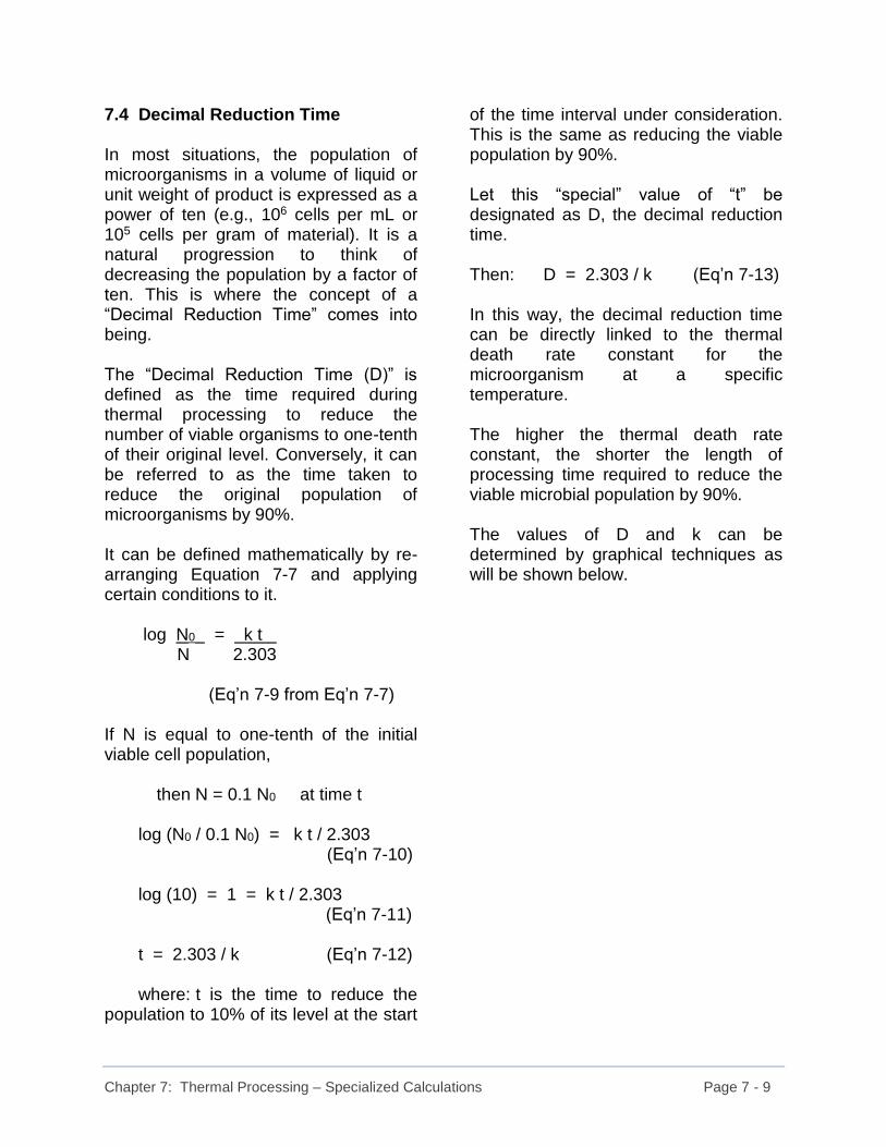
Chapter 7: Thermal Processing – Specialized Calculations Page 7 - 9
7.4 Decimal Reduction Time In most situations, the population of microorganisms in a volume of liquid or unit weight of product is expressed as a power of ten (e.g., 106 cells per mL or 105 cells per gram of material). It is a natural progression to think of decreasing the population by a factor of ten. This is where the concept of a “Decimal Reduction Time” comes into being. The “Decimal Reduction Time (D)” is defined as the time required during thermal processing to reduce the number of viable organisms to one-tenth of their original level. Conversely, it can be referred to as the time taken to reduce the original population of microorganisms by 90%. It can be defined mathematically by re-arranging Equation 7-7 and applying certain conditions to it. log N0 = k t N 2.303 (Eq’n 7-9 from Eq’n 7-7) If N is equal to one-tenth of the initial viable cell population, then N = 0.1 N0 at time t log (N0 / 0.1 N0) = k t / 2.303 (Eq’n 7-10) log (10) = 1 = k t / 2.303 (Eq’n 7-11) t = 2.303 / k (Eq’n 7-12) where: t is the time to reduce the population to 10% of its level at the start
of the time interval under consideration. This is the same as reducing the viable population by 90%. Let this “special” value of “t” be designated as D, the decimal reduction time. Then: D = 2.303 / k (Eq’n 7-13) In this way, the decimal reduction time can be directly linked to the thermal death rate constant for the microorganism at a specific temperature. The higher the thermal death rate constant, the shorter the length of processing time required to reduce the viable microbial population by 90%. The values of D and k can be determined by graphical techniques as will be shown below.
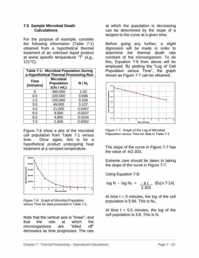
Chapter 7: Thermal Processing – Specialized Calculations Page 7 - 10
7.5 Sample Microbial Death Calculations For the purpose of example, consider the following information (Table 7-1) obtained from a hypothetical thermal treatment of an unknown liquid product at some specific temperature “T” (e.g., 121°C).
Table 7-1: Microbial Population During a Hypothetical Thermal Processing Run
Time (minutes)
Microbial Population (cfu / mL)
N / No
0 460,000 1.00
0.5 320,000 0.696
1.5 150,000 0.326
3.0 49,000 0.107
4.0 21,000 0.0457
5.0 9,500 0.0207
6.0 4,800 0.0104
7.0 2,400 0.0052
Figure 7-6 show a plot of the microbial cell population from Table 7-1 versus time. Once again, this is for a hypothetical product undergoing heat treatment at a constant temperature.
Figure 7-6: Graph of Microbial Population versus Time for data presented in Table 7-1.
Note that the vertical axis is “linear”, and that the rate at which the microorganisms are “killed off” decreases as time progresses. The rate
at which the population is decreasing can be determined by the slope of a tangent to the curve at a given time. Before going any further, a slight digression will be made in order to determine the thermal death rate constant of the microorganism. To do this, Equation 7-8 from above will be employed. By plotting the “Log of Cell Population versus Time”, the graph shown as Figure 7-7 can be obtained.
Figure 7-7: Graph of the Log of Microbial Population versus Time for data in Table 7-1.
The slope of the curve in Figure 7-7 has the value of -k/2.303. Extreme care should be taken in taking the slope of the curve in Figure 7-7. Using Equation 7-8: log N - log N0 = - k t (Eq’n 7-14) 2.303 At time t = 0 minutes, the log of the cell population is 5.66. This is N0. At time t = 5.5 minutes, the log of the cell population is 3.8. This is N.
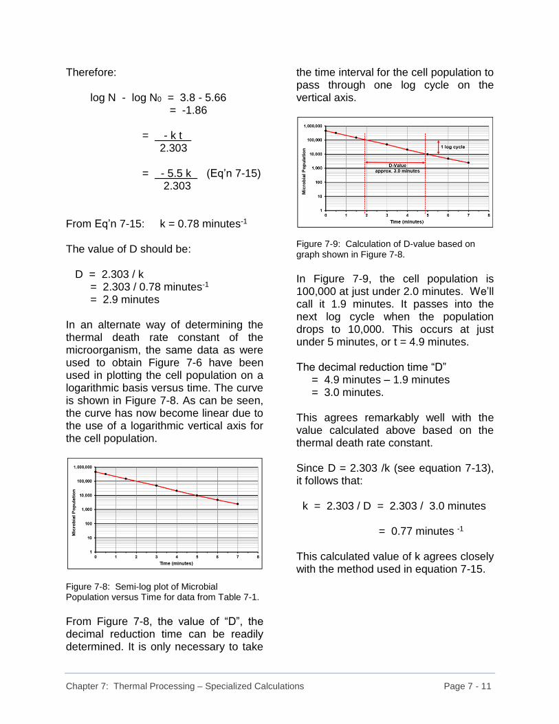
Chapter 7: Thermal Processing – Specialized Calculations Page 7 - 11
Therefore: log N - log N0 = 3.8 - 5.66 = -1.86 = - k t 2.303 = - 5.5 k (Eq’n 7-15) 2.303 From Eq’n 7-15: k = 0.78 minutes-1 The value of D should be: D = 2.303 / k = 2.303 / 0.78 minutes-1 = 2.9 minutes In an alternate way of determining the thermal death rate constant of the microorganism, the same data as were used to obtain Figure 7-6 have been used in plotting the cell population on a logarithmic basis versus time. The curve is shown in Figure 7-8. As can be seen, the curve has now become linear due to the use of a logarithmic vertical axis for the cell population.
Figure 7-8: Semi-log plot of Microbial Population versus Time for data from Table 7-1.
From Figure 7-8, the value of “D”, the decimal reduction time can be readily determined. It is only necessary to take
the time interval for the cell population to pass through one log cycle on the vertical axis.
Figure 7-9: Calculation of D-value based on graph shown in Figure 7-8.
In Figure 7-9, the cell population is 100,000 at just under 2.0 minutes. We’ll call it 1.9 minutes. It passes into the next log cycle when the population drops to 10,000. This occurs at just under 5 minutes, or t = 4.9 minutes. The decimal reduction time “D” = 4.9 minutes – 1.9 minutes = 3.0 minutes. This agrees remarkably well with the value calculated above based on the thermal death rate constant. Since D = 2.303 /k (see equation 7-13), it follows that: k = 2.303 / D = 2.303 / 3.0 minutes = 0.77 minutes -1 This calculated value of k agrees closely with the method used in equation 7-15.

Chapter 7: Thermal Processing – Specialized Calculations Page 7 - 12
7.6 Sterilization Criteria As previously stated, the sterilization criteria is essentially the number of log cycles by which the initial population of a microorganism must be decreased to reach a desired final microbial population. It would be ideal to have absolutely no microorganisms present after heat treating a product. However, this is not statistically possible. Example Problem: Consider the following example of a liquid product packaged in a 355 mL can: Assume 106 microorganisms per millilitre present in a product prior to sterilization. (Even if the microbial population is 105 / mL, using 106 will give an added safety margin.) The processor is prepared to accept a risk of one spoiled can of product in every 100,000. (This may not be realistic for an actual production environment, but it is only for example purposes here). The processor can tolerate 1 microorganism in 100,000 cans; or: Volume = 100,000 cans | 355 mL | can = 35,500,000 mL Therefore, the final cell population is 1 cell per 35,500,000 mL (or 2.82 x 10⁻⁸ cells/mL).
The sterilization criteria = ln N0 = ln ( 106 ) N ( 2.82 x 10⁻⁸) = ln (0.355 x 10¹⁴) = 31.2 Recall, from Eq’n 7-5a: ln (N0 / N) = k t Therefore, kt = 31.2 From this, it follows that: t = 31.2 / k If the contaminating microorganism is G. stearothermophilus, the following sterilization times would be needed at the indicated temperatures, using the rate constants listed in Table 7-7. t = 31.2 / k at 100°C, k = 0.019 min-1 (From Table 7-2) t = 31.2 . 0.019 min-1 = 1642.1 minutes ≈ 27.4 hours ≈ 1.14 days 1.14 days is an excessively long time period. Other time intervals can be calculated for other temperatures and the most appropriate time and temperature combination can then be selected for the
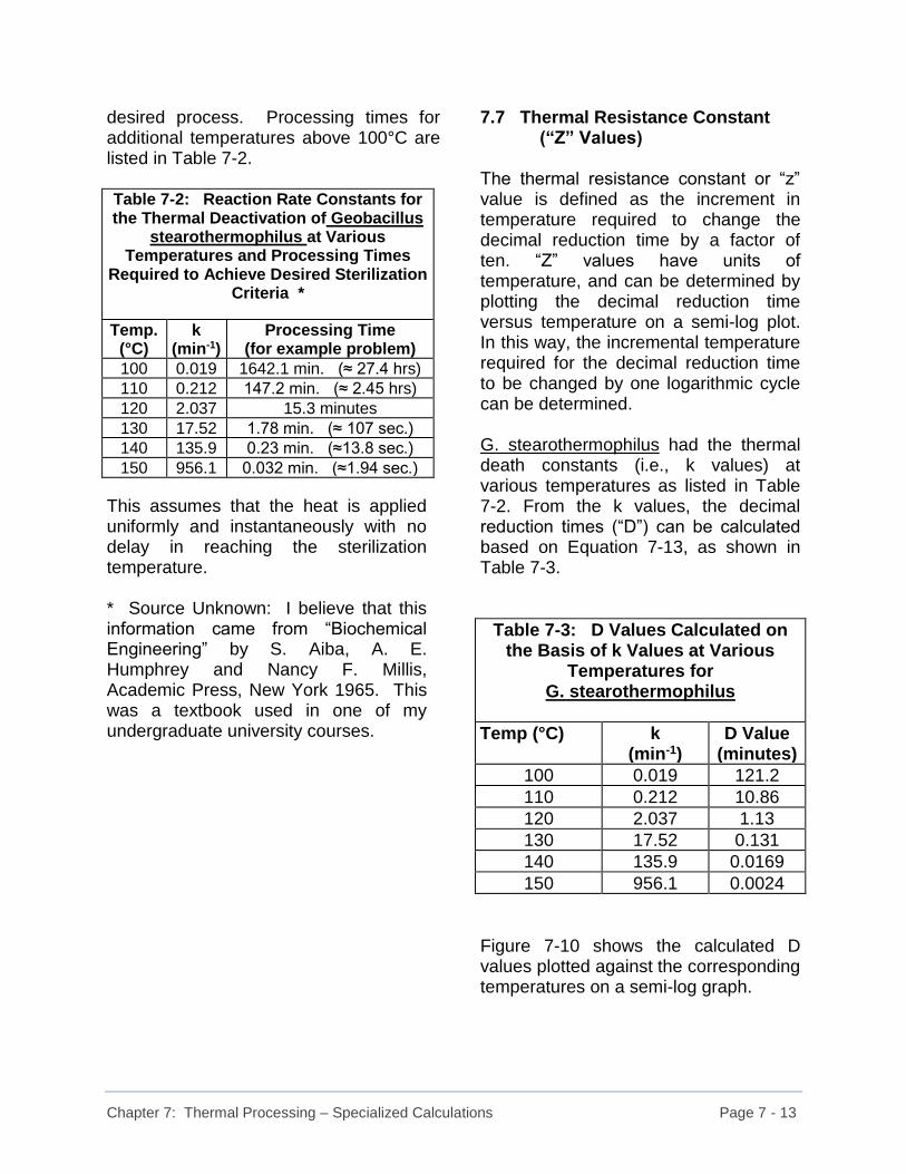
Chapter 7: Thermal Processing – Specialized Calculations Page 7 - 13
desired process. Processing times for additional temperatures above 100°C are listed in Table 7-2. Table 7-2: Reaction Rate Constants for the Thermal Deactivation of Geobacillus
stearothermophilus at Various Temperatures and Processing Times
Required to Achieve Desired Sterilization Criteria *
Temp. (°C)
k (min-1)
Processing Time (for example problem)
100 0.019 1642.1 min. (≈ 27.4 hrs)
110 0.212 147.2 min. (≈ 2.45 hrs)
120 2.037 15.3 minutes
130 17.52 1.78 min. (≈ 107 sec.)
140 135.9 0.23 min. (≈13.8 sec.)
150 956.1 0.032 min. (≈1.94 sec.)
This assumes that the heat is applied uniformly and instantaneously with no delay in reaching the sterilization temperature. * Source Unknown: I believe that this information came from “Biochemical Engineering” by S. Aiba, A. E. Humphrey and Nancy F. Millis, Academic Press, New York 1965. This was a textbook used in one of my undergraduate university courses.
7.7 Thermal Resistance Constant (“Z” Values) The thermal resistance constant or “z” value is defined as the increment in temperature required to change the decimal reduction time by a factor of ten. “Z” values have units of temperature, and can be determined by plotting the decimal reduction time versus temperature on a semi-log plot. In this way, the incremental temperature required for the decimal reduction time to be changed by one logarithmic cycle can be determined. G. stearothermophilus had the thermal death constants (i.e., k values) at various temperatures as listed in Table 7-2. From the k values, the decimal reduction times (“D”) can be calculated based on Equation 7-13, as shown in Table 7-3.
Table 7-3: D Values Calculated on the Basis of k Values at Various
Temperatures for G. stearothermophilus
Temp (°C) k (min-1)
D Value (minutes)
100 0.019 121.2
110 0.212 10.86
120 2.037 1.13
130 17.52 0.131
140 135.9 0.0169
150 956.1 0.0024
Figure 7-10 shows the calculated D values plotted against the corresponding temperatures on a semi-log graph.

Chapter 7: Thermal Processing – Specialized Calculations Page 7 - 14
Figure 7-10: Plot of Decimal Reduction Time versus Temperature for Geobacillus stearothermophilus.
Figure 7-10 may be described as a thermal resistance curve for a particular microorganism. In this case, the microorganism is G. stearothermophilus. Based on Figure 7-10, the z value for G. stearothermophilus can be determined as the temperature increment required to lower the decimal reduction time by one log cycle (see Figure 7-11). This is approximately 10.5° (on the Celsius scale) from the data presented. This means that for every 10.5° increase in temperature from a specific reference point, the decimal reduction time is reduced by a factor of ten. Conversely, for every 10.5 C° drop in temperature from a specific reference point, the decimal reduction time will increase by a factor of ten.
Figure 7-11: Determination of Z-value using graph shown in Figure 7-10.
As an example, consider a product which must be processed for one hour at 125°C. If the temperature was increased by 10.5 C° to 135.5°C, the processing would take only 0.1 hours, or 6 minutes. If the temperature was reduced by 10.5 C° to 114.5°C, the product would have to be processed for 10 hours to receive the same degree of kill. This assumes that the time for heat penetration is not a factor. A large z value indicates that microorganism is relatively resistant to increases in temperature. A smaller z value indicates that the microbial population is more susceptible to the effects of heating. The significance of z values may be illustrated in HTST (high temperature short time) thermal processing. In HTST processes, the temperatures may be around 95°C and the holding times could be about 20 seconds; whereas if the temperature could be raised to 121°C, the processing time could be reduced to just a few seconds. This is one reason why ultra-high temperature (UHT) processes are so attractive in that they allow for extremely short processing times at very high temperatures (e.g., 150°C).

Chapter 7: Thermal Processing – Specialized Calculations Page 7 - 15
7.8 Thermal Death Time (“F” Values) The thermal death time for a process can be defined as the time required to achieve a stated reduction in the population of a microorganism at a specified temperature. Thermal death times have units of “time” (e.g., minutes) as their name so obviously implies. The most important thing to remember is that this is the time required to obtain a “stated reduction” in the microbial population. It can be the reduction necessary to bring an initial cell population down to a “safe” level below some arbitrarily established threshold level. This is all done at a specified temperature. For sample purposes, consider an initial solution containing 500 cfu per mL (i.e., colony forming units per millilitre) of G. stearothermophilus. This solution or product is to be packed in 500 mL cans and the processor is willing to accept one spoiled can in one million. The target population would then be 1 cfu per 1,000,000 cans. The volume of one million cans would be 500 mL/can times one million cans which is equal to 500 million mL. This means that we can only allow one colony forming unit to be present in 5 x 10⁸ mL. That gives us a final concentration of 1 cfu / 5 x 10⁸ mL or 2 x 10⁻⁹ cfu per mL. A plot of microbial population versus time (on a semi-log plot) would result in a graph similar to that shown in Figure 7-12.
Figure 7-12: Plot of Log cfu/mL versus time for sample problem.
The D value for G. stearothermphilus is about 1.13 minutes at 120°C based on the information presented in Table 7-3 slope. This means it that it would take approximately 1.13 minutes for the population to decrease by one log cycle in Figure 7-12. It is apparent from Figure 7-12 that the desired target population is not achieved until the product had been exposed to a temperature of 120°C for approximately 13 minutes. Therefore, the F-value for this particular process at 120°C is 13 minutes. It is also interesting to note that the F value or thermal death time is equivalent to approximately 11.5 decimal reduction times, or about 12 thermal death times if the value is rounded off to the nearest whole number. This would give a 12D process for the product. In Figure 7-12, the curve passes through approximately 12 log cycles (11.5 cycles, actually) or 12 decimal reduction times as the microbial population drops from its initial value to its final value. Hence the expression that this is a 12D process. In typical commercial sterilizations, processes are established to handle Clostridium botulinum and the most
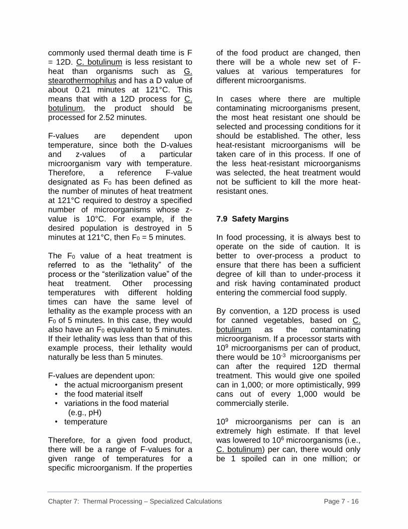
Chapter 7: Thermal Processing – Specialized Calculations Page 7 - 16
commonly used thermal death time is F = 12D. C. botulinum is less resistant to heat than organisms such as G. stearothermophilus and has a D value of about 0.21 minutes at 121°C. This means that with a 12D process for C. botulinum, the product should be processed for 2.52 minutes. F-values are dependent upon temperature, since both the D-values and z-values of a particular microorganism vary with temperature. Therefore, a reference F-value designated as F0 has been defined as the number of minutes of heat treatment at 121°C required to destroy a specified number of microorganisms whose z-value is 10°C. For example, if the desired population is destroyed in 5 minutes at 121°C, then F0 = 5 minutes. The F0 value of a heat treatment is referred to as the “lethality” of the process or the “sterilization value” of the heat treatment. Other processing temperatures with different holding times can have the same level of lethality as the example process with an F0 of 5 minutes. In this case, they would also have an F0 equivalent to 5 minutes. If their lethality was less than that of this example process, their lethality would naturally be less than 5 minutes. F-values are dependent upon: • the actual microorganism present • the food material itself • variations in the food material (e.g., pH) • temperature Therefore, for a given food product, there will be a range of F-values for a given range of temperatures for a specific microorganism. If the properties
of the food product are changed, then there will be a whole new set of F-values at various temperatures for different microorganisms. In cases where there are multiple contaminating microorganisms present, the most heat resistant one should be selected and processing conditions for it should be established. The other, less heat-resistant microorganisms will be taken care of in this process. If one of the less heat-resistant microorganisms was selected, the heat treatment would not be sufficient to kill the more heat-resistant ones. 7.9 Safety Margins In food processing, it is always best to operate on the side of caution. It is better to over-process a product to ensure that there has been a sufficient degree of kill than to under-process it and risk having contaminated product entering the commercial food supply. By convention, a 12D process is used for canned vegetables, based on C. botulinum as the contaminating microorganism. If a processor starts with 109 microorganisms per can of product, there would be 10-3 microorganisms per can after the required 12D thermal treatment. This would give one spoiled can in 1,000; or more optimistically, 999 cans out of every 1,000 would be commercially sterile. 109 microorganisms per can is an extremely high estimate. If that level was lowered to 106 microorganisms (i.e., C. botulinum) per can, there would only be 1 spoiled can in one million; or

Chapter 7: Thermal Processing – Specialized Calculations Page 7 - 17
999,999 cans out of a million would be sterile. There are added safeguards when dealing with acidic foods (pH values below 4.6). Most microorganisms do not grow well in acidic media and the spores of C. botulinum do not germinate at such low pH levels. The following factors will influence microbial growth in heat treated canned products:
• the species of microorganisms in the microbial population
• acidity of the product • ability of the population to grow in
anaerobic environments • water activity of the product (lower
Aw’s protect spores) • thermal resistance of the food itself • etc.
7.10 Spoilage Probability Heldman and Hartel (1997) have detailed the use of a “spoilage probability” equation that determines the number of cans of a product that may be produced with no more than one spoiled container. The relationship is: 1 = N0 (Eq’n 7-16) r 10 (F/D) where: r = number of containers of processed product N0 = initial population of spoilage microorganisms per container F = thermal death time required (i.e., the F-value) D = decimal reduction time For a sample calculation, let’s consider the case of G. stearothermophilus at 120°C, with 500 microorganisms per mL in a 500 mL can. The initial microbial population would be 250,000 microorganisms per can (i.e., 500 microorganisms per mL times 500 mL per can = 2.5 x 10⁵ microorganisms per can). We can restate this by saying that there are 250,000 colony forming units, or “cfu’s”, per can. The cans are to be held at 120°C for 13 minutes (this is the F-value). Based on information presented earlier in this chapter (see Table 7-3) the D-value is 1.13 minutes.
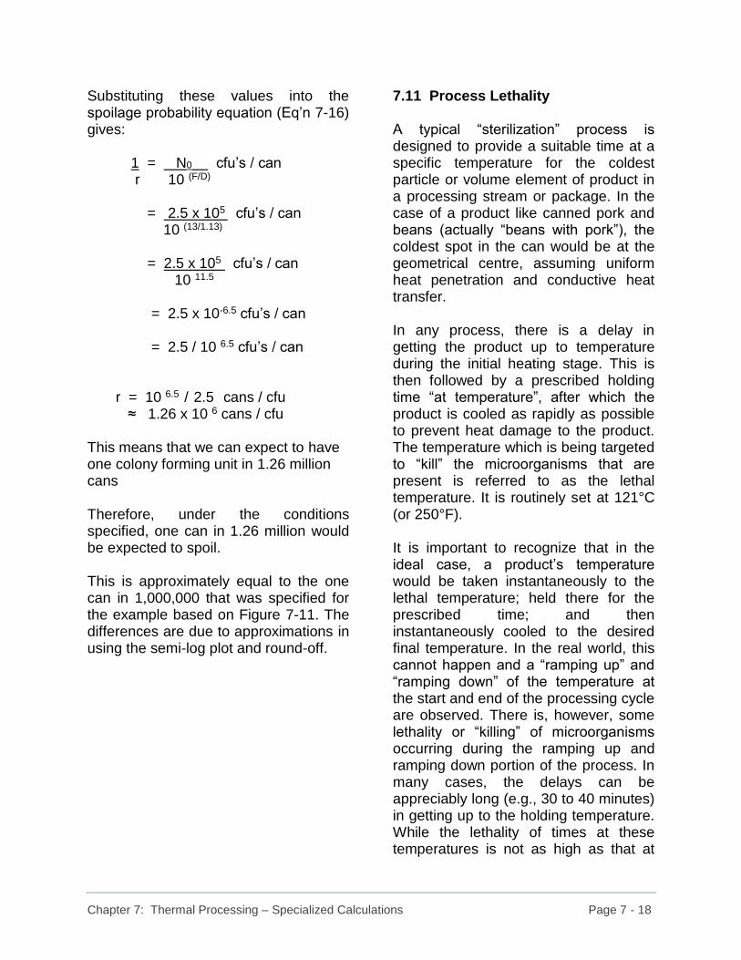
Chapter 7: Thermal Processing – Specialized Calculations Page 7 - 18
Substituting these values into the spoilage probability equation (Eq’n 7-16) gives: 1 = N0 cfu’s / can r 10 (F/D) = 2.5 x 10⁵ cfu’s / can 10 (13/1.13) = 2.5 x 10⁵ cfu’s / can 10 11.5 = 2.5 x 10-6.5 cfu’s / can = 2.5 / 10 6.5 cfu’s / can r = 10 6.5 / 2.5 cans / cfu ≈ 1.26 x 10 6 cans / cfu This means that we can expect to have one colony forming unit in 1.26 million cans Therefore, under the conditions specified, one can in 1.26 million would be expected to spoil. This is approximately equal to the one can in 1,000,000 that was specified for the example based on Figure 7-11. The differences are due to approximations in using the semi-log plot and round-off.
7.11 Process Lethality A typical “sterilization” process is designed to provide a suitable time at a specific temperature for the coldest particle or volume element of product in a processing stream or package. In the case of a product like canned pork and beans (actually “beans with pork”), the coldest spot in the can would be at the geometrical centre, assuming uniform heat penetration and conductive heat transfer. In any process, there is a delay in getting the product up to temperature during the initial heating stage. This is then followed by a prescribed holding time “at temperature”, after which the product is cooled as rapidly as possible to prevent heat damage to the product. The temperature which is being targeted to “kill” the microorganisms that are present is referred to as the lethal temperature. It is routinely set at 121°C (or 250°F). It is important to recognize that in the ideal case, a product’s temperature would be taken instantaneously to the lethal temperature; held there for the prescribed time; and then instantaneously cooled to the desired final temperature. In the real world, this cannot happen and a “ramping up” and “ramping down” of the temperature at the start and end of the processing cycle are observed. There is, however, some lethality or “killing” of microorganisms occurring during the ramping up and ramping down portion of the process. In many cases, the delays can be appreciably long (e.g., 30 to 40 minutes) in getting up to the holding temperature. While the lethality of times at these temperatures is not as high as that at
Chapter 7: Thermal Processing – Specialized Calculations Page 7 - 19
121°C for a similar time, they should be factored into the overall lethality of the process. In order to include times at lower temperatures in the lethality of a process, the concept of a “unit of lethality” can be employed. One “unit of lethality” can be defined as the amount of heat kill equivalent to one minute at 121°C for a microorganism with a given z-value. Fractions of a minute at 121°C, or their equivalents, correspond to fractions of a unit of lethality. The fractions of a unit of lethality are often referred to as “lethal rates”. The lethal rate can be defined by the relationship (Heldman & Hartel, 1997): Lethal Rate = 10 (T - TR)/z (Eq’n 7-17) where: T = temperature of product TR = reference temperature (e.g., 121°C) z = z-value for microorganism By taking the temperature at regular intervals, during the thermal processing of a product, the lethal rates can be calculated. They can than be plotted against time to obtain a “lethal rate vs time” curve for the process. The area under the curve (in minutes) will give the equivalent lethality of the process or Fo of the process. In a basic batch pasteurization process for milk, the milk must be exposed to a temperature of 63°C for 30 minutes. Using the relationship that one unit of lethality equals one minute at 63°C, the basic pasteurization process requires 30 units of lethality or 30 minutes.
If the thermal process was to use a higher temperature, the time could be shortened, but the lethality of the process must still be equal to or greater than 30 minutes. With an HTST process at 71.5°C, a reference temperature of 63°C, and a z-value of 4.1C° for the microorganisms present, the lethal rates can be calculated as: LR = 10 (T-TR)/z = 10 (71.5 - 63) / 4.1 = 102.07 = 117.5 (Eq’n 7-18) It now remains to calculated the time required with a lethal rate of 117.5 at 71.5°C that is equivalent to 30 minutes at a lethal rate of 1.0. Let the required time at 71.5°C be “t” The process lethality would be117.5 t But this lethality must be equal to a process lethality of 30 minutes which was the lethality of the batch pasteurization process. Therefore, 117.5 t = 30 minutes Solving for t gives: t = 0.255 minutes = 15.3 seconds. This means that a retention time of 15.3 seconds at 71.5°C would be equivalent to the basic batch pasteurization process for milk. As stated earlier, in an HTST process, the established conditions for milk pasteurization are 71.5°C for 15 seconds, which is approximately what has been derived here.

Chapter 7: Thermal Processing – Specialized Calculations Page 7 - 20
By rounding the temperature up to 72°C, the lethal rate would become 156.7. The required retention time would be reduced to 0.2 minutes, or 12 seconds. It could then be said that by processing milk for 15 seconds at 72°C, the necessary pasteurization requirements would be exceeded. This slight increase in temperature would have no deleterious effects on the quality of the milk, and would give the added insurance that the product had been adequately heat treated. Going to a UHT process with a temperature of 150°C, the lethal rate becomes LR = 10 (T-TR)/z = 10 (150 - 63) / 4.1 = 1021.2 = 1.6 x 10²¹ (Eq’n 7-19) This lethal rate is so large that it makes even a fraction of a second sufficient to provide the same lethality as was obtained from 30 minutes at 63°C. In most continuous processes, it is not possible to measure retention times lower than 1 or 2 seconds, so a 1 or 2 second retention time is routinely used. There does not need to be a significantly long holding tube (the length is flowrate dependent) for these short retention times and the product quality is not seriously damaged by such high temperatures for these brief intervals.
7.12 Calculation of F-values at Different Temperatures Once again, consider the batch pasteurization of milk. It required 30 minutes of holding time at a reference temperature of 63°C for a microorganism with a z-vale of 4.1C°. Using the equation for Lethal Rate, Lethal Rate = LR = 10 (T-TR)/z (Eq’n 7-17 from above) The lethal rate at the reference temperature, is determined as being 1.0, since 100 = 1.0. For the pasteurization process at 63°C, the F-value is specified as being 30 minutes. If the temperature is changed, the required holding time will also need to be changed. This new holding time will be the new F-value for the modified process. The new F-value must give the same (or better) overall lethality to the processing as the original F-value at the reference temperature. Therefore: F-value at reference temperature = Time at reference temperature = Lethal Rate at x Time at New Temp. New Temp. = Lethal Rate at x F-value at New Temp. New Temp.
(Eq’n 7-20)

Chapter 7: Thermal Processing – Specialized Calculations Page 7 - 21
This assumes a step change in temperature (both up and down) with little or no lethality occurring outside of the actual time that the milk is spending at its pasteurization temperature. But, the time at the new temperature is the new F-value. Using this knowledge and substituting it and Equation 7-17 into Equation 7-20, it follows: Fref = Fnew x 10 (T-TR)/z
(Eq’n 7-21) Re-arranging Equation 7-21 gives: Fnew = Fref .
10 (T-TR)/z = Fref x 10 -(T-TR)/z or: Fnew = Fref x 10 (TR-T)/z (Eq’n 7-22) where: TR = reference temperature for the process When calculating the new holding time for a pasteurization process at 71.5°C, the following values would be substituted into Equation 7-22: TR = Reference Temperature = 63°C T = new temperature of product = 71.5°C z = Z value of microorganisms = 4.1 C° Fref = processing time at ref. temp. = 30 minutes
This gives: Fnew = Fref x 10 (TR-T)/z = 30 minutes x 10 (63 - 71.5) / 4.1 = 30 minutes x 10 -2.073 = 0.253 minutes = 15.2 seconds Allowing for round-off differences, this result is comparable to the result calculated previously.

Chapter 7: Thermal Processing – Specialized Calculations Page 7 - 22
7.13 An Alternate Way of Looking at Z-values It was previously stated that z-values are the temperature changes required to change the D-value of a microorganism by a factor of ten. Referring to Figure 7-11, take the specific case of where z is the temperature increment from 120.5°C to 131°C. This corresponds to a one decade or one log cycle decrease in the D-value. By taking any temperature change and dividing it by the number of log cycles through which the corresponding D-values pass, one can determine the z-value for the system under consideration. At a temperature T = T1, the D value will be DT1 At a temperature T = T2, the D value will be DT2 , where T2 is the higher temperature. Since T2 is the higher temperature, DT2 will be lower than DT1. The temperature difference = T2 - T1 The number of log cycles through which the temperature range passes would be (Singh & Heldman, 1993): log DT1 - log DT2 Therefore: Z = T2 - T1 log DT1 - log DT2 (Eq’n 7-23) For example: We can use Figure 7-11 to illustrate this method. Let’s select two
temperatures from Figure 7-11 which has been reproduced as Figure 7-13 below.
Figure 7-13: Using Figure 7-11 to illustrate alternate way of calculating Z values.
At T1 = 105°C: D ≈ 35 minutes
At T2 = 135°C: D ≈ 0.045 minutes
These values can now be substituted into Equation 7-23 for Z: Z = T2 - T1 log DT1 - log DT2 = 135°C - 105°C . log (35) – log (0.045) = 30 C° . 1.544 – (-1.347) = 30 C° / 2.891 = 10.4 C° This value is in extremely close agreement with that calculated based on one log cycle in Figure 7-11 (i.e., Z = 10.5 C°). The small difference can be attributed to reading values off the respective graphs.

Chapter 7: Thermal Processing – Specialized Calculations Page 7 - 23
7-14 Summary Comments In this chapter, we have covered some of the more specialized, or advanced, calculations relating to thermal processing. Depending upon your situation, you may or may not find the information presented here relevant. For those who are examining thermal processing from a more academic perspective, this material may be of more interest than to those who wish to gain an appreciation of the basics of thermal processing. 7-15 References Aiba,S., A. E. Humphrey and Nancy F. Millis, “Biochemical Engineering” Academic Press, New York, 1965. Heldman, Dennis R., and Richard W. Hartel. “Principles in Food Processing”; Aspen Publication, Springer, New York, 1997. Singh, R. Paul, and Dennis R. Heldman. “Introduction to Food Engineering” (Fifth Edition); Academic Press, London, 2014.

Chapter 8: Basics of Drying Food Materials Page 8 - 1
8. Basics of Drying Food Materials 8.1 Introduction Drying of food products, or “dehydration” as it is also known, is something that many consumers take for granted. Most people are familiar with dried soup mixes, “instant” potato flakes, dried fruit pieces in trail mixes or packaged cereals, and a host of other dried materials - yet they may be tempted to dismiss drying as “just taking the water out”. However, hidden beneath the apparent simplicity of this water removal is a complex scientific discipline that is all-too-often ignored in food processing. Removing water from food products is not simply a matter of applying heat and waiting until the moisture content is lowered to some desired final level. As will be shown, there are numerous factors to be considered. While progressing through this section, try to envision different food products that are commonly available, and how drying may have had an impact on them. Experience gained through non-food related drying applications in a person’s everyday life can often be applied to understanding food drying processes. Even something as mundane as drying a load of clothing in an automatic clothes dryer can offer insight into some aspects of drying technology. Although the end products may be significantly different, there are often many similarities among various drying applications. It should be kept in mind that food processing frequently involves the translation of skills or knowledge learned in one area to a new, less familiar activity.
8.2 Reasons for Drying Food Products The main reason for drying food products is to reduce their spoilage. Microbial spoilage often results when moisture levels within a particular product are high enough to support the growth of various microorganisms. Other forms of spoilage, such as the development of off-flavours can occur in the presence of high moisture levels over the course of time. Going hand-in-hand with the reduction of food spoilage is the enhancement of the storage life of a product. By removing appropriate amounts of water, the shelf-life can be extended and the need for specialized storage conditions can be minimized. Materials that would require frozen or refrigerated storage conditions when in their original state may be stored at room temperature for significantly longer periods of time. Even under refrigerated conditions (ca. 4°C), non-dehydrated products may only remain usable for periods of a few days to several weeks. As the global economy expands, and processors begin to take advantage of emerging world markets, shipping and handling constraints can become important factors. Removal of water from a product reduces its overall weight and often its volume, thereby making it more economical to ship such products to distant locations. An example of this would be dried tomatoes. Fresh tomatoes generally contain up to 95% water by weight. This means that 100 kg of fresh tomatoes would contain 95 kg of water and only 5 kg of solids (i.e., the remaining 5% is solids). When

Chapter 8: Basics of Drying Food Materials Page 8 - 2
dried, the tomatoes would contain 10% moisture and the remaining 90% would be solids. The weight of dried tomatoes obtained from the initial 100 kg would be about 5.6 kg (Figure 8-1). The drying process has reduced the weight by approximately 94.4 kg. Not only has the shipping weight been reduced, but the volume has been substantially reduced as well. Of course, we must take into consideration the desired end use of the tomatoes. Dried tomatoes have a somewhat more limited use than fresh tomatoes, but are ideal for stews and similar dishes.
Figure 8-1: Reduction in weight of tomatoes by water removal
Water removal has certainly created a feature of added convenience to many products. Dehydrated potato flakes (Figure 8-2) offer the consumer the convenience of a “just add water and stir” approach to meal preparation. Not only is the quality very high, but the preparation time for peeling, paring, and cooking the potatoes is eliminated.
Figure 8-2: Dehydrated potato flakes offer convenience and portion control.
Portion control is also enhanced through use of such products. Waste elimination or reduction is also an attractive benefit through being able to prepare what you need when you need it. While consumers often appreciate the convenience of these products, they also demand extremely high quality which is often higher than they would expect from what they would prepare in their own home. Drying can also change the inherent attributes of food products as well as alter performance characteristics. Plums may be dried to form prunes, or grapes can be dried to create raisins (Figure 8-3).
Figure 8-3: Plums and grapes can be changed to prunes and raisins by drying.

Chapter 8: Basics of Drying Food Materials Page 8 - 3
Herbs like parsley can have the water removed to form dried parsley flakes for use as seasonings (Figure 8-4). The list goes on and on.
Figure 8-4: Removing water from fresh parsley gives dried parsley flakes for seasoning.
8.3 Historical Development of Food
Drying The actual origins of food drying or dehydration date back to pre-recorded history. The discovery of drying as a preservation technique was probably quite accidental. Early hunters and gatherers may have found that berries which had dried naturally on vines or shrubs still retained their flavour and palatability even when fresh berries were no longer available. Indigenous North Americans prepared “pemmican” from strips of lean meat dried by hanging them over open fires. The meat was then pounded into a paste and mixed with fat, or suet, and dried berries. Once pressed into small cakes, the pemmican served as a source of food when fresh food and game was not readily available. Early explorers also used pemmican. It is reported that the first recorded food drying was for vegetables during the 18th Century (Barbosa-Canovas and Vega-Mercado, 1996). As is often the case, advances in technology are often
catalysed by potential military applications. Food dehydration was no exception. During the Crimean War which was fought from 1854 to 1856, British troops were supplied with dried vegetables which were processed back in Britain. During the Boer War (1899 to 1902), dried vegetables were shipped from Canada to South Africa; and during World War I, over 4,500 tons of dried vegetables were sent to Europe from the United States. According to Barbosa-Canovas and Vega-Mercado (1996), mechanical hot-air dryers were developed in the late 1800's and early 1900's to replace sun drying, and specialty dryers were designed to allow for the dehydration of milk and egg products. Other methods of drying such as “salting” have also been used. Packing food such as fish in salt crystals can withdraw water, but leaves a very high salt content in the food itself. This makes it necessary to soak the fish in fresh water to extract as much of the salt as possible before consuming it. Today, many dried foods can be found on supermarket shelves thanks to developments in dryer design and drying technology that are described in this section.
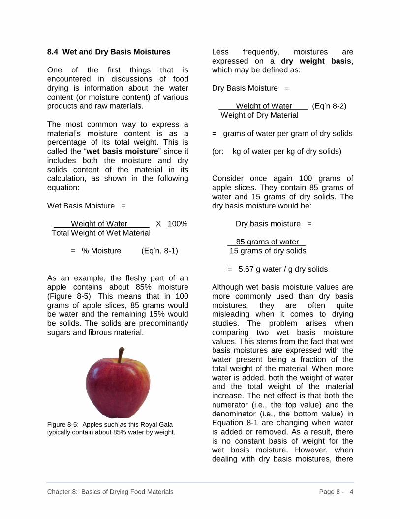
Chapter 8: Basics of Drying Food Materials Page 8 - 4
8.4 Wet and Dry Basis Moistures One of the first things that is encountered in discussions of food drying is information about the water content (or moisture content) of various products and raw materials. The most common way to express a material’s moisture content is as a percentage of its total weight. This is called the “wet basis moisture” since it includes both the moisture and dry solids content of the material in its calculation, as shown in the following equation: Wet Basis Moisture = Weight of Water X 100% Total Weight of Wet Material = % Moisture (Eq’n. 8-1) As an example, the fleshy part of an apple contains about 85% moisture (Figure 8-5). This means that in 100 grams of apple slices, 85 grams would be water and the remaining 15% would be solids. The solids are predominantly sugars and fibrous material.
Figure 8-5: Apples such as this Royal Gala typically contain about 85% water by weight.
Less frequently, moistures are expressed on a dry weight basis, which may be defined as: Dry Basis Moisture = Weight of Water (Eq’n 8-2) Weight of Dry Material = grams of water per gram of dry solids (or: kg of water per kg of dry solids) Consider once again 100 grams of apple slices. They contain 85 grams of water and 15 grams of dry solids. The dry basis moisture would be: Dry basis moisture = 85 grams of water . 15 grams of dry solids = 5.67 g water / g dry solids Although wet basis moisture values are more commonly used than dry basis moistures, they are often quite misleading when it comes to drying studies. The problem arises when comparing two wet basis moisture values. This stems from the fact that wet basis moistures are expressed with the water present being a fraction of the total weight of the material. When more water is added, both the weight of water and the total weight of the material increase. The net effect is that both the numerator (i.e., the top value) and the denominator (i.e., the bottom value) in Equation 8-1 are changing when water is added or removed. As a result, there is no constant basis of weight for the wet basis moisture. However, when dealing with dry basis moistures, there

Chapter 8: Basics of Drying Food Materials Page 8 - 5
is a constant basis of comparison since the moisture content is expressed as the weight of water contained per unit weight of dry material. Figure 8-6 shows the relationship between wet basis and dry basis moistures.
Figure 8-6: Graph of wet basis moisture versus dry basis moisture.
Figure 8-7 shows a close-up view of what we see in Figure 8-6 above. This time, however, we will examine the relationship between wet basis and dry basis moistures in more detail. The focus is now on the dry basis moistures from 0 grams of water per gram of dry solids, which is often referred to as “bone dry”, to 7 grams of water per gram of dry solids. Looking at Figure 8-7, it can be seen that 1 gram of water per gram of dry solids is equivalent to 50% wet basis moisture, which can be calculated by substituting the values of 1 gram of water and 2 grams total weight into Equation 8-1. The addition of this single gram of water to one gram of dry solids increases the wet basis moisture content from 0% to 50%. This is shown as “❶” in Figure 8-7.
Figure 8-7: A closer look at the relationship between wet basis moistures and dry basis moistures. If an additional gram of water was added to one gram of dry solids, the wet basis moisture content would be 66.7% (i.e., 2 grams of water in 3 grams total weight of material). This second gram of water raised the wet basis moisture content from 50% to 66.7%, which is an increase of about 16.7%. Adding a third gram of water to the gram of dry solids would give a wet basis moisture content of 75%, for and increase of approximately 8.3% over the previous moisture content. If a fourth gram of water was added to the original one gram of dry solids, the wet basis moisture content would rise to 80% (i.e., 4 grams of water in 5 grams of total material). The contribution in moisture increase by adding this fourth gram of water would only be 5% from the case where there were 3 grams of water per gram of dry solids. This final water addition is shown as “❷” in Figure 8-7.
As can be seen, when making stepwise additions of water in equal increments to a gram of dry solids, the corresponding amount of change in the wet basis moisture decreases. Initially, a 50% increase in wet basis moisture was obtained by adding 1 gram of water to a

Chapter 8: Basics of Drying Food Materials Page 8 - 6
gram of dry solids; but there was only a 5% increase in the wet basis moisture when a gram of water was added to a gram of dry solids that already contained 3 grams of water in the last step considered above. Following several sample calculations of wet and dry basis moistures, the full impact of these observations will be explored in a brief “Case Study”. 8.4.1 Sample Calculations Sample Question 8-1: A sweet potato (Figure 8-8) has a moisture content of 70% on a wet basis. Convert this moisture to its equivalent dry basis moisture.
Figure 8-8: Sweet potato with a moisture content of 70% on a wet basis.
Solution: Since no initial weight of material is given, assume a weight of 100 grams. The actual weight itself is unimportant when working with percentages for the wet basis moisture and on a “per unit weight” basis for the dry basis moistures. 100 grams was chosen as a convenient starting value upon which to base subsequent calculations.
If 70% of the material is water (i.e., 70% moisture on a wet basis), then it would be safe to consider that the remaining 30% would be solids since no other liquid components are specified. The percentages can be converted to their decimal fraction equivalents for use in the necessary calculations. In 100 grams of material, we have: Weight of water = 100 g x 0.70 = 70 grams Weight of solids = 100 g x 0.30 = 30 grams Dry basis moisture = weight of water . weight of dry material = 70 g water . 30 g dry solids = 2.33 g water / g dry solids Therefore, the dry basis moisture is 2.33 grams of water per gram of dry solids. 100 kg could also have been selected for a starting weight. The answer would have been 2.33 kilograms of water per kilogram of dry solids. These answers are equivalent. When using 100 grams (or 100 kg) as the basis for a calculation, there is probably no need to go through the detailed calculations for weights of water and solids. These can be done quickly without the use of a calculator.

Chapter 8: Basics of Drying Food Materials Page 8 - 7
Sample Question 8-2: What are the wet basis and dry basis moistures obtained by mixing 35 kg of water with 90 kg of totally dry powdered starch (Figure 8-9)?
Figure 8-9: Dry powdered starch in plastic tub.
Solution: The first thing that must be done is to determine the weight of water and dry solids present in the total mixture. In this case, the answers to this question are quite straight-forward. Weight of water = 35 kg Weight of dry solids = 90 kg Total weight of the mixture = weight of water + weight of dry solids = 35 kg + 90 kg = 125 kg Wet basis moisture = weight of water x 100% total weight of mixture = 35 kg x 100% 125 kg = 28%
Dry basis moisture = weight of water . weight of dry solids = 35 kg water . 90 kg dry solids = 0.39 kg of water / kg dry solids Therefore, the wet basis moisture content is 28% and the dry basis moisture content is 0.39 kg of water per kg of dry solids. Question 8-3: What are the wet and dry basis moistures resulting from mixing 25 kg of water with 18 kg of flour containing 12% moisture? Solution: This problem is similar to Question 8-2, except for the fact that the flour being used here contains some water. Therefore, it is necessary to determine the amount of water and solids present in the flour before proceeding with the moisture calculations. In 18 kg of flour, there is 12% water and 88% solids (i.e., 100% - % water) Weight of water in flour = 18 kg x 0.12 = 2.16 kg Weight of solids in flour = 18 kg x 0.88 = 15.84 kg or:
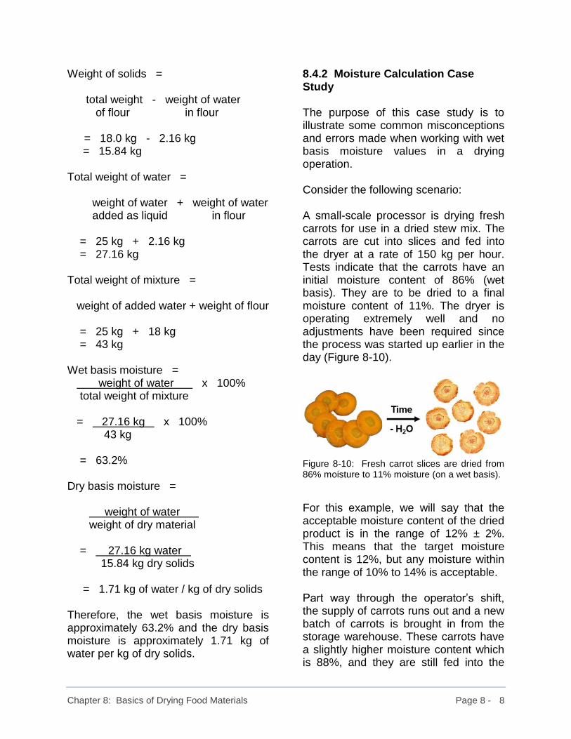
Chapter 8: Basics of Drying Food Materials Page 8 - 8
Weight of solids = total weight - weight of water of flour in flour = 18.0 kg - 2.16 kg = 15.84 kg Total weight of water = weight of water + weight of water added as liquid in flour = 25 kg + 2.16 kg = 27.16 kg Total weight of mixture = weight of added water + weight of flour = 25 kg + 18 kg = 43 kg Wet basis moisture = weight of water x 100% total weight of mixture = 27.16 kg x 100% 43 kg = 63.2% Dry basis moisture = weight of water . weight of dry material = 27.16 kg water . 15.84 kg dry solids = 1.71 kg of water / kg of dry solids Therefore, the wet basis moisture is approximately 63.2% and the dry basis moisture is approximately 1.71 kg of water per kg of dry solids.
8.4.2 Moisture Calculation Case Study The purpose of this case study is to illustrate some common misconceptions and errors made when working with wet basis moisture values in a drying operation. Consider the following scenario: A small-scale processor is drying fresh carrots for use in a dried stew mix. The carrots are cut into slices and fed into the dryer at a rate of 150 kg per hour. Tests indicate that the carrots have an initial moisture content of 86% (wet basis). They are to be dried to a final moisture content of 11%. The dryer is operating extremely well and no adjustments have been required since the process was started up earlier in the day (Figure 8-10).
Figure 8-10: Fresh carrot slices are dried from 86% moisture to 11% moisture (on a wet basis).
For this example, we will say that the acceptable moisture content of the dried product is in the range of 12% ± 2%. This means that the target moisture content is 12%, but any moisture within the range of 10% to 14% is acceptable. Part way through the operator’s shift, the supply of carrots runs out and a new batch of carrots is brought in from the storage warehouse. These carrots have a slightly higher moisture content which is 88%, and they are still fed into the

Chapter 8: Basics of Drying Food Materials Page 8 - 9
dryer at 150 kg per hour. The quality control technician asks the operator if any adjustments are going to be made to the dryer, but is told that no adjustments are necessary. The operator reasons that since the moisture content of the carrots coming into the dryer has increased by only 2.0%, the final moisture should increase by only 2.0% as well. The additional 2.0% will increase the final moisture content of the dried carrots to 13% which is still below the allowable upper moisture limit of 14%. The QC technician tries to convince the operator to monitor the process very closely in order to avoid overly damp product, but the operator tells the technician not to worry so much. An hour or so later, the operator cannot believe the results of the latest moisture test and has several hundred kilograms of “out of spec” product. What was the final moisture content of the second batch of carrots and what was wrong with the operator’s initial logic that no changes were needed for the dryer? Solution: The first thing to do when starting any problem is to draw a diagram showing all available information and identifying unknowns. Figure 8-11 shows the initial drying conditions.
Figure 8-11: Diagram of conditions for initial batch of carrots in drying “Case Study”.
From Figure 8-11, we can see that we need to identify how much water was removed during the drying process to give the desired finished product moisture of 11%. To do this, the amount of water present in the carrots at the start and end of the drying process must be calculated, and the difference between the two will determine how much water was removed. Before beginning, it is also necessary to take care of the “time” factor. Since all processing rates are expressed on a “per hour” basis, 1 hour would be suitable as the basis for any calculations, and will allow for the use 150 kg rather than “150 kg per hour” in the calculations. Basis = 1 hour of operation. Weight of water in carrots entering dryer = 150 kg x 0.86 = 129 kg Weight of solids in carrots entering dryer = 150 kg - 129 kg water = 21 kg The next step is to determine how much water is in the dried carrot slices. However, there is no mention in the

Chapter 8: Basics of Drying Food Materials Page 8 - 10
problem statement about the weight of carrot slices obtained from the process. Looking at Figure 8-11, the only loss in the process appears to be the water removed in the dryer. No loss of solids is mentioned. Therefore, it would be considered safe to assume that the weight of solids leaving the dryer would be the same as the weight of solids entering the dryer, which is 21 kg on an hourly basis. Weight of carrot solids leaving dryer = Weight of carrot solids entering dryer = 21 kg The carrot slices leaving the dryer contain 11% water by weight. This means that they must contain 89% solids by weight (i.e., 100% - % water). Since the actual weight of the dried carrot slices is unknown, let their weight be X kg. Then, 89% of the X kg will be the weight of solids, which is 21.0 kg. 0.89 X = 21 kg Solving for X gives: X = 21 kg = 23.6 kg 0.89 Since 21 kg of the final product is dry solids, the weight of water in the final product must be: Weight of water in dried carrots = Weight of dried - Weight of dry product solids = 23.6 kg - 21.0 kg = 2.6 kg
The weight of the water removed can now be calculated. Weight of water removed = Weight of water - Weight of water at start at end = 129 kg - 2.6 kg = 126.4 kg. This means that the dryer is set up to remove 126.4 kg of water per hour from the carrot slices that are fed through it. Now, attention must be directed to the new batch of carrot slices coming into the dryer. They have an initial moisture content of 88% and are metered into the dryer at a rate of 150 kg per hour just as was done to the first batch. Figure 8-12 summarizes what is known about the second batch of carrot slices.
Figure 8-12: Diagram of conditions for second batch of carrots in drying “Case Study”.
Weight of water in carrots entering dryer = 150 kg x 0.88 = 132 kg Weight of solids in carrots entering dryer = 150 kg - 132 kg water = 18 kg
Chapter 8: Basics of Drying Food Materials Page 8 - 11
At this point, it is important to reflect on what is known about the process to be able to determine how the final water content of the finished product can be calculated. The dryer has been running under conditions suitable for the first batch of carrots and is set up to remove 126.4 kg of water each hour. This is the key factor for solving the problem of how much water will be left in the second batch of carrot slices. Therefore, the weight of water removed from second batch of carrot slices = 126.4 kg Water left in second batch of carrot slices = Weight of water in - Weight of water second batch removed = 132 kg - 126.4 kg = 5.6 kg It is now known that 5.6 kg of water are contained in 18 kg of dry carrot solids. This is the weight of dry solids entering the dryer in the second batch of carrot slices. Total weight of product in second batch of carrot slices = Weight of water + Weight of dry solids in product in product = 5.6 kg + 18 kg = 23.6 kg There is now enough information available to calculate the final wet basis moisture content of the second batch of dried carrot slices.
Wet basis moisture = weight of water x 100% total weight of product = 5.6 kg x 100% 23.6 kg = 23.7% Based upon a moisture content of 23.7%, it is easy to understand the process operator’s surprise. Not only is this more than 10% higher than the operator expected, but it is well above the allowable upper moisture limit of 14% for the product. The reason for the operator’s error in judgement was the assumption that wet basis moistures behave “linearly”. It was assumed that the amount of water contributing to a moisture difference of 2.0% at levels around 86% moisture would be the same as the amount of water contributing to a moisture difference of 2.0% at levels around 11% moisture. From Figure 8-7 and the subsequent discussion of it, it is apparent that this is really not the case.

Chapter 8: Basics of Drying Food Materials Page 8 - 12
8.4.3 Comparing Moisture Contents Table 8-1 lists the water contents of a number of fruits and vegetables on both a wet basis and a dry basis.
Table 8-1: Water Contents of Selected Fruits and Vegetables
Sample Wet Basis Moisture *
(%)
Dry Basis (g water /
g dry solids)
Apple 84.7% (84%) 5.54
Banana 72.0% (75%) 2.57
Cantaloupe 87.4% (92%) 6.94
Carrots 87.8% (88%) 7.20
Celery 95.6% (94%) 21.7
Mangoes 81.9% (81%) 4.52
Peas (Green) 79.8% (74%) 3.95
Pineapple 84.1% (84%) 5.29
Tomatoes 93.8% (94%) 15.1
Watermelon 91.9% (93%) 11.4
Non-bracketed values are personal data (D.Mercer) Literature values for wet basis moistures are in parentheses (ASHRAE, 1986)
The values in Table 8-1 are based on actual tests done by the author in the laboratory, and have been expressed to three significant digits. The experimental values have then been compared to literature values which are meant to be representative of typical moisture contents. While the experimentally determined data are in relatively close agreement with the literature values, there are some differences between
them that may be somewhat upsetting at first. However, there are quite valid reasons for these differences. Reasons for these variations include: • differences in the variety of the fruits
or vegetables • variations in growing conditions • variations in storage conditions and
length of storage time • location of sample taken from
parent material • number of observations included in
determining moisture content Care must be taken to understand when to use actual experimental data and literature values. In cases where tests are being done on a specific batch of material, it is important to determine the actual moisture content of that material. When conducting drying trials on samples from three or four apples, it would be imperative to know how much water was in those particular apples. This means that small samples of the apples would have to be tested. However, if someone was required to do calculations for a non-specific product sample, then using representative literature values as a starting point would be quite appropriate. In this way, it would be possible to determine approximately how much water was in a metric tonne of apples of a non-specific variety, grown under average growing conditions, and subjected to average storage conditions. Average literature values are more appropriate for general calculations than laboratory results based on a small sample population from a small number of growing and storage conditions. For
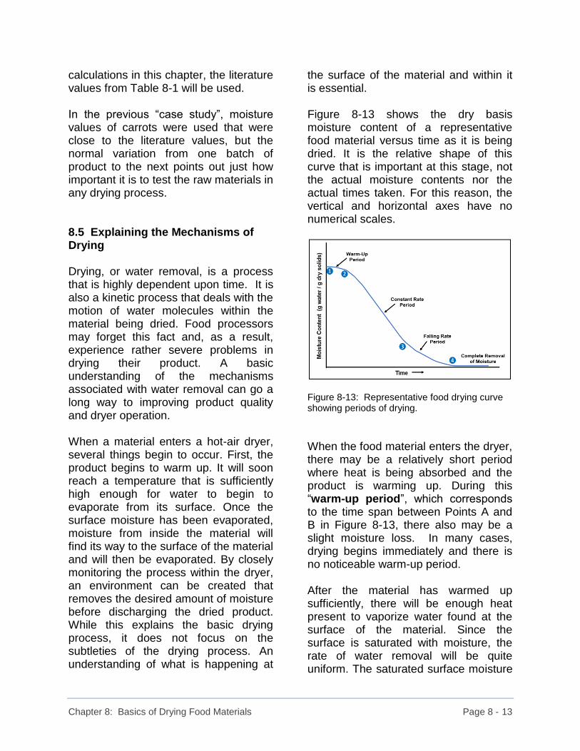
Chapter 8: Basics of Drying Food Materials Page 8 - 13
calculations in this chapter, the literature values from Table 8-1 will be used. In the previous “case study”, moisture values of carrots were used that were close to the literature values, but the normal variation from one batch of product to the next points out just how important it is to test the raw materials in any drying process. 8.5 Explaining the Mechanisms of Drying Drying, or water removal, is a process that is highly dependent upon time. It is also a kinetic process that deals with the motion of water molecules within the material being dried. Food processors may forget this fact and, as a result, experience rather severe problems in drying their product. A basic understanding of the mechanisms associated with water removal can go a long way to improving product quality and dryer operation. When a material enters a hot-air dryer, several things begin to occur. First, the product begins to warm up. It will soon reach a temperature that is sufficiently high enough for water to begin to evaporate from its surface. Once the surface moisture has been evaporated, moisture from inside the material will find its way to the surface of the material and will then be evaporated. By closely monitoring the process within the dryer, an environment can be created that removes the desired amount of moisture before discharging the dried product. While this explains the basic drying process, it does not focus on the subtleties of the drying process. An understanding of what is happening at
the surface of the material and within it is essential. Figure 8-13 shows the dry basis moisture content of a representative food material versus time as it is being dried. It is the relative shape of this curve that is important at this stage, not the actual moisture contents nor the actual times taken. For this reason, the vertical and horizontal axes have no numerical scales.
Figure 8-13: Representative food drying curve showing periods of drying.
When the food material enters the dryer, there may be a relatively short period where heat is being absorbed and the product is warming up. During this “warm-up period”, which corresponds to the time span between Points A and B in Figure 8-13, there also may be a slight moisture loss. In many cases, drying begins immediately and there is no noticeable warm-up period. After the material has warmed up sufficiently, there will be enough heat present to vaporize water found at the surface of the material. Since the surface is saturated with moisture, the rate of water removal will be quite uniform. The saturated surface moisture

Chapter 8: Basics of Drying Food Materials Page 8 - 14
pool will remain present as long as there is a sufficient flow of moisture from inside the wet material to replace any moisture lost at the surface due to evaporation. This is called the “constant rate period” and corresponds to the time between Points B and C in Figure 8-13. The linear nature of this portion of the curve indicates the constant rate at which moisture is being removed, which is how this drying period got its name. Another way of looking at it is to consider that the slope of the curve is constant over this entire period. A calculation of the slope of the line during the constant drying rate period will give the weight of water evaporated per unit weight of dry solids per unit time (e.g., g water per g dry solids per minute, or per hour). Eventually, evaporation of the surface moisture will progress to a point where moisture from inside the material cannot reach the surface quickly enough to replenish the surface moisture pool. When this happens, the surface is no longer saturated. Now, moisture diffuses through pores in the material from its inner regions to the surface where it is evaporated by the hot air in the dryer. As more and more water is removed, the diffusion process becomes slower and slower, and the rate at which the water is removed decreases proportionately. During this stage of drying, moisture removal is diffusion-controlled, and the drying mechanism is in its “falling rate period”. This is shown in Figure 8-13 as the portion of the curve between Points C and D. Moving along the curve from Point C to Point D, the slope of the curve
decreases, which indicates that the rate of water removal is decreasing. Just as in the case of the constant rate period, the slope of the curve during the falling rate period has units of weight of water evaporated per unit weight of dry solids per unit time. As time progresses, these values get smaller and smaller during the falling rate period and will ultimately approach a rate of zero grams of water per gram of dry solids per minute. In some food products, all moisture present can be evaporated if the drying time is sufficient. In other products, there may be some water still remaining in the product because it is bound tightly within the food’s matrix structure. The bound water may not be removed under gentle drying conditions and will remain as an integral part of the food as it leaves the drying process. Figure 8-14 shows a plot of dry basis moisture versus time for hot yellow peppers cut lengthwise into quarters. They are being dried at 50°C with an air velocity of 0,5 metres per second. Notice that there is no warm-up period. Instead, the drying goes right into the constant rate drying period which lasts about 1.5 hours.
Figure 8-14: Dry basis moisture versus time for the drying of hot yellow pepper slices at 50°C and an air velocity of 0.5 m/s.

Chapter 8: Basics of Drying Food Materials Page 8 - 15
The moisture content where the drying mechanism switches from the constant rate period to the falling rate period is often referred to as the “critical moisture content”. For the hot yellow pepper drying in Figure 8-14, the critical moisture content was around 8.0 grams of water per gram of dry solids, or about 88.9% wet basis moisture. The initial moisture content of the hot yellow peppers was 12.7 grams of water per gram of dry solids which is equivalent to 92.7% on a wet basis. It took approximately 16 hours for the moisture content of the pepper slices to reach 10% on a wet basis, or 0.11 grams of water per gram of dry solids on a dry basis.
8.6 Factors Influencing Drying: There are many factors that influence the rate of water removal from a product, or how long a particular material takes to dry. Ultimately the product’s final quality can be greatly affected. One way of looking at these factors is to divide them into two categories: product-related attributes, and dryer-related attributes. 8.6.1 Product-Related Attributes Product composition and structure often differ from one material to another. These characteristics can change with the amount of heat and moisture that are present. As an example, cereal grain products such as wheat or rice are composed primarily of starches (Figure 8-15).
Figure 8-15: Ungelatinized rice kernels leaving a milling process.
In some processes, moisture is added to the grain to enhance its processing properties. With the addition of water, the starch matrix, or network, of the kernels begins to swell. When sufficient heat is added, the starch gelatinizes. After processing, it is then necessary to

Chapter 8: Basics of Drying Food Materials Page 8 - 16
remove this added water. During drying, moisture must diffuse out of the swollen starch matrix which behaves much differently than would be the case if we were to dry the ungelatinized non-swollen kernels. Other materials such as herbs and spices dry differently than pasta products, or fruits and vegetables. Each product has its own inherent characteristics which make it extremely important to understand and optimize the drying conditions for that product. Figure 8-16 shows how the drying of hot yellow peppers differs from the drying of fresh oregano. The concept of “moisture ratios” will be explained later.
Figure 8-16: The drying properties of hot yellow peppers and fresh oregano are quite different even when dried under the same conditions.
Surface characteristics play an important role in the drying of foods. It is often difficult to remove moisture from berries which have a waxy layer on their surface (Figure 8-17). Nature has intended the fleshy part of berries to provide protection and future nourishment for the seeds inside the berry. Moisture loss is definitely not desirable in this case. However, when
processors want to dry berries, they are faced with this surface barrier to water removal and must take measures to overcome it such as slicing the berry or breaking the surface in several places.
Figure 8-17: Fresh cranberries have a waxy outer layer or “cuticle” that prevents moisture from escaping.
Rough or pitted surfaces may offer the opportunity for easier moisture removal since there may be access to many pores that go into the interior of the material and allow the escape of moisture by rapid diffusion to the surface. Particle size is a rather obvious attribute that can affect water removal. With large particles, the distance that moisture must travel from the centre to the outer surface is greater than for smaller particles. As a result, it takes longer for the moisture to reach the surface in the larger particles, and they dry more slowly than their smaller counterparts (Figure 8-18).

Chapter 8: Basics of Drying Food Materials Page 8 - 17
Figure 8-18: Moisture can travel from the centre to the surface of the sphere with the smaller radius “r” faster than it can in the larger sphere with the radius “R”.
Particle shape can also impact the rate of water removal during drying. There are generally three basic shapes that are considered in most drying treatments: spheres, cylinders, and flat plates (Figure 8-19).
Figure 8-19: There are three basic shapes considered in drying.
Each characteristic shape offers its own unique drying behaviour. Examples of spherical particles would be peas or Brussel sprouts and the like. With spheres, moisture must travel from the centre in a direction along a radius of the sphere to reach the surface where it can be evaporated.
Whole carrots, spaghetti noodles, or rice grains might be considered as examples of cylindrical materials. In these cases of cylinders, we tend to ignore the ends of the cylinder and consider that moisture must travel from the centre of the cylinder along a radial axis to get to the surface. Slices of fruit and vegetables, or wide flat pasta products, would be considered as flat plates for the purpose of drying. With flat plates or “slabs”, we generally ignore moisture loss through the edges of the material and focus on losses from the top and bottom surfaces. Moisture must travel from the centre of the flat plate or “slab” to either surface before it is evaporated. The actual mathematics of how different material shapes affect drying will not be discussed here. Porosity is another player in determining how rapidly materials dry. As mentioned above (see “Surface Characteristics”), materials with pores extending down into their interior have a route that will allow easier diffusion of moisture to the surface. If pores are sufficiently large, hot air may actually be able to penetrate into them and take the drying process right down into the core of the material rather than just having it occur at the outer surface. The porous nature of apple slices which contain many air sacs contributes greatly to their rapid moisture loss during drying (Figure 8-20).
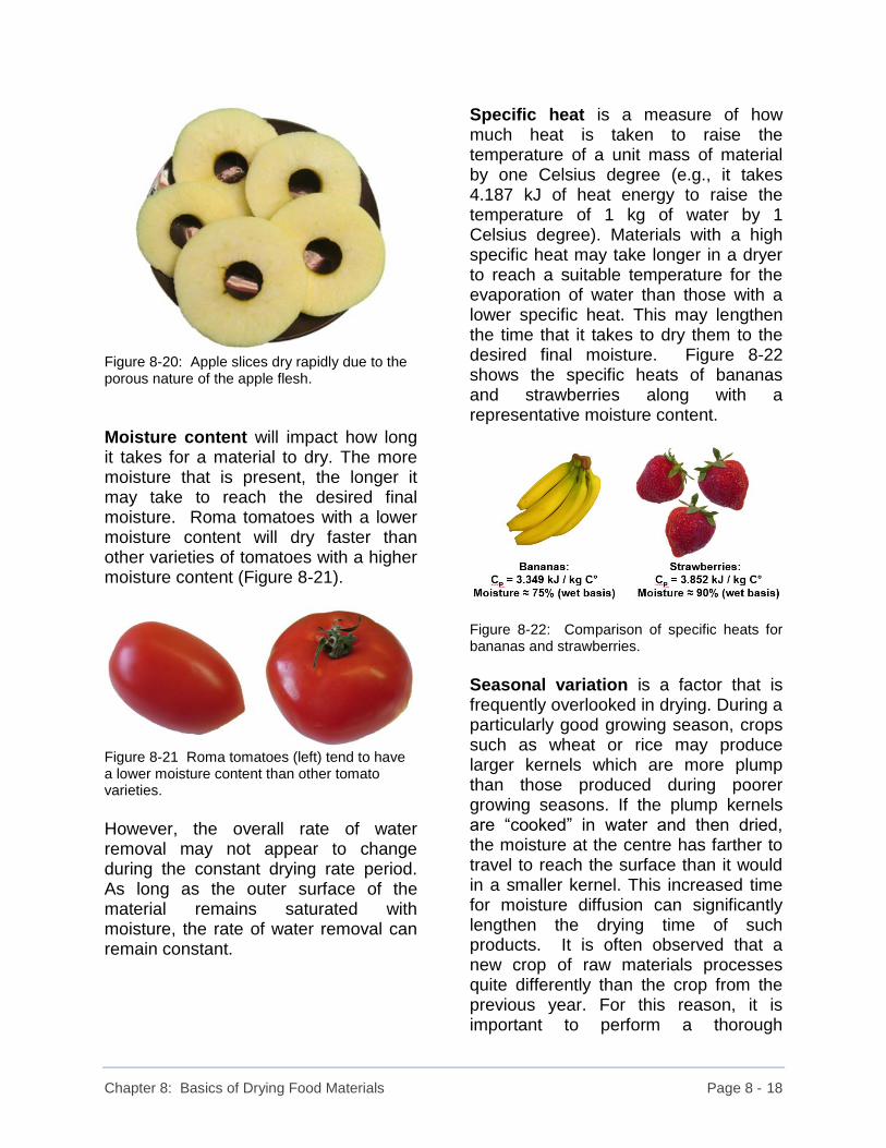
Chapter 8: Basics of Drying Food Materials Page 8 - 18
Figure 8-20: Apple slices dry rapidly due to the porous nature of the apple flesh.
Moisture content will impact how long it takes for a material to dry. The more moisture that is present, the longer it may take to reach the desired final moisture. Roma tomatoes with a lower moisture content will dry faster than other varieties of tomatoes with a higher moisture content (Figure 8-21).
Figure 8-21 Roma tomatoes (left) tend to have a lower moisture content than other tomato varieties. However, the overall rate of water removal may not appear to change during the constant drying rate period. As long as the outer surface of the material remains saturated with moisture, the rate of water removal can remain constant.
Specific heat is a measure of how much heat is taken to raise the temperature of a unit mass of material by one Celsius degree (e.g., it takes 4.187 kJ of heat energy to raise the temperature of 1 kg of water by 1 Celsius degree). Materials with a high specific heat may take longer in a dryer to reach a suitable temperature for the evaporation of water than those with a lower specific heat. This may lengthen the time that it takes to dry them to the desired final moisture. Figure 8-22 shows the specific heats of bananas and strawberries along with a representative moisture content.
Figure 8-22: Comparison of specific heats for bananas and strawberries.
Seasonal variation is a factor that is frequently overlooked in drying. During a particularly good growing season, crops such as wheat or rice may produce larger kernels which are more plump than those produced during poorer growing seasons. If the plump kernels are “cooked” in water and then dried, the moisture at the centre has farther to travel to reach the surface than it would in a smaller kernel. This increased time for moisture diffusion can significantly lengthen the drying time of such products. It is often observed that a new crop of raw materials processes quite differently than the crop from the previous year. For this reason, it is important to perform a thorough
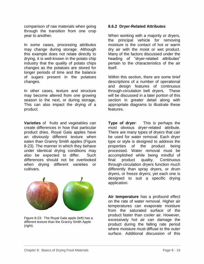
Chapter 8: Basics of Drying Food Materials Page 8 - 19
comparison of raw materials when going through the transition from one crop year to another. In some cases, processing attributes may change during storage. Although this example does not relate directly to drying, it is well-known in the potato chip industry that the quality of potato chips changes as the potatoes are stored for longer periods of time and the balance of sugars present in the potatoes changes. In other cases, texture and structure may become altered from one growing season to the next, or during storage. This can also impact the drying of a product. Varieties of fruits and vegetables can create differences in how that particular product dries. Royal Gala apples have an obviously different texture when eaten than Granny Smith apples (Figure 8-23). The manner in which they behave under identical drying conditions may also be expected to differ. Such differences should not be overlooked when drying different varieties or cultivars.
Figure 8-23: The Royal Gala apple (left) has a different texture than the Granny Smith Apple (right).
8.6.2 Dryer-Related Attributes When working with a majority or dryers, the principal vehicle for removing moisture is the contact of hot or warm dry air with the moist or wet product. Many of the factors discussed under the heading of “dryer-related attributes” pertain to the characteristics of the air itself. Within this section, there are some brief descriptions of a number of operational and design features of continuous through-circulation belt dryers. These will be discussed in a later portion of this section in greater detail along with appropriate diagrams to illustrate these features. Type of dryer: This is perhaps the most obvious dryer-related attribute. There are many types of dryers that can be used for water removal. Each dryer type or style is designed to address the properties of the product being processed. Water removal must be accomplished while being mindful of final product quality. Continuous through-circulation dryers function much differently than spray dryers, or drum dryers, or freeze dryers; yet each one is designed to suit a specific drying application. Air temperature has a profound effect on the rate of water removal. Higher air temperatures can evaporate moisture from the saturated surface of the product faster than cooler air. However, excessively hot air can damage the product during the falling rate period where moisture must diffuse to the outer surface. Additional discussion of this

Chapter 8: Basics of Drying Food Materials Page 8 - 20
topic appears under “Impact of Drying on the Product”. Heat sources often dictate the temperatures to which air can be heated for use in the dryer. If natural gas is available, air can be heated to extremely high temperatures (e.g., over 200°C or over 400°F) by directly passing the air to be heated through a bank of flames as in a gas-fired furnace or oven. However, in instances when natural gas is not available, heating of the air may be done by passing the air over metal tubes or coils containing steam. Pressure limitations may allow steam temperatures to reach only as high as 125°C or 150°C (ca. 255°F to 300°F). As a result, air temperatures may only reach these temperatures and will be less effective at drying than higher temperature air streams. Care must be taken when using these excessively hot temperatures as they can damage the product. They should only be used in specialized cases and for large-scale drying operations. In general, most food products are best dried at temperatures around 50°C to 55°C. Relative humidity of the air is another concern. Relative humidity is an indication of the amount of moisture present in the air at a given temperature compared to the amount of water that could be held by that air if it was saturated with moisture. Air with a low relative humidity has the potential to pick up more moisture than air with a higher relative humidity at that same temperature. Heating air to a higher temperature helps lower its relative
humidity and enhance its ability to pick up moisture in the dryer. Let’s consider the example of air at 20°C that has a relative humidity of 60%. From psychrometric charts, we can find the actual, or absolute, water content of the air. Under these conditions, the air is holding 10.4 grams of water per kg of dry air. This is 60% of the moisture that it can possibly hold. Now, let’s take the air with 60% relative humidity at 20°C and heat it to 55°C. It will still contain 10.4 grams of water per kilogram of air. At 55°C, the air is able to hold much more moisture and a water content of 10.4 grams of water per kg dry air equates to a relative humidity of only 10%. This tells us that the air at 55°C has the potential to take up more moisture than when it was at only 20°C. Relative humidities are measured using hygrometers. Many of these are electronic, providing rapid reliable readings (Figure 8-24).
Figure 8-24: This electronic hygrometer indicates that the relative humidity of the air at 23°C is 34% and that the air is considered “dry”.

Chapter 8: Basics of Drying Food Materials Page 8 - 21
Psychrometric charts are somewhat complicated to explain in a brief overview such as this. Basically, they provide us with a method of determining the various properties of air that contains water vapour under a wide variety of conditions. Should you wish to find detailed information on their use, there are on-line resources available. Water removal capacity of the air is an important consideration in drying. We have just seen how heating the air reduces its relative humidity (RH), even though the absolute water content of the air has remained constant. We can expand on this thought process and calculate how much water the air is capable of removing at a given temperature. Using a psychrometric chart, we found that there were 10.4 grams of water in every kilogram of dry air at 20°C and 60% relative humidity. We can also find how much water the air is capable of holding if it is fully saturated with moisture. At 20°C, air can hold a maximum of 17.3 grams of water per kg of dry air. This means that it is saturated with moisture and has a relative humidity of 100%. If we were to use this air in a drying process, the maximum amount of water that it could possibly remove would be the difference between how much water it is actually holding and how much water it could possibly hold when saturated. We can put this into the form of an equation as follows:
Maximum water removal capacity = Maximum amount - Actual amount of water air can of water air is hold holding Maximum water removal capacity for air at 20°C = 17.3 g H2O - 10.4 g H2O per kg dry air per kg dry air = 6.9 g H2O per kg dry air Let’s compare this to the same starting air (20°C and 60% RH) if we heat the air to 55°C. At 55°C, the heated air has a relative humidity of 10% and still contains 10.4 grams of water per kg of dry air. However, if heated to 55°C, the air can hold 104.7 grams of water per kg dry air at saturation (i.e., 100% RH). We can now calculate its maximum water removal capacity. Maximum water removal capacity for air at 55°C = 104.7 g H2O - 10.4 g H2O per kg dry air per kg dry air = 94.3 g H2O per kg dry air The difference between these two maximum water removal capacities clearly indicates how much more effective heated air is at removing moisture than cooler air. The maximum water removal capacity values are generally not attainable in a typical food dryer. However, these values do provide us with an indication of the theoretical maximum amount of

Chapter 8: Basics of Drying Food Materials Page 8 - 22
water that could be removed by the heated air. Volumetric flowrate of air is an indication of the volume of air delivered to a dryer per unit time (e.g., the number of cubic metres of air per minute). It is linked to the temperature of the air and is directly responsible for the amount of heat that is delivered to a dryer. Since the heat content of air is expressed as the number of kiloJoules of heat energy per kg of air (or per cubic metre of air under a given set of temperature and pressure conditions), the hotter the air, the greater the amount of heat it will contain per unit weight or volume. In addition, the greater the amount of hot air delivered to the dryer, the greater the amount of heat that is available for evaporating moisture from the product being dried. In a very wet product, it may be quite acceptable to deliver a large volume of air at a high temperature to evaporate as much water as rapidly as possible. This approach should only be used during the constant rate drying period when there is sufficient moisture at the product surface to remove water without damaging the product. My personal preference is to use the same air temperature throughout the entire drying process. In this way, there is no danger of forgetting to reduce the temperature at the end of the constant rate period, which will potentially damage the product during the falling rate drying period.
Linear velocity of the air goes hand-in-hand with the volumetric flowrate of air in most dryer systems. Since most dryers are constructed with fixed-size dimensions, if the volumetric flowrate of air going into a dryer is increased, the linear velocity of the air will increase as well. Linear velocity is a measure of the forward speed of the air and is measured in units of distance per unit time (e.g., metres per second, etc.). It may be measured in a number of ways, including the use of a vaned anemometer. The higher the linear air velocity, the faster the anemometer spins. Figure 8-25 shows a vaned anemometer with a linear velocity of 0.48 metres per second indicated.
Figure 8-25: A linear air velocity of 0.48 m/s is indicated on this vaned anemometer.
Linear velocity is an important factor in drying, since fast-moving air can physically lift pieces of product inside the dryer and upset the drying uniformity. If linear velocities are too high, particles of product may even be carried right out of the dryer and become a processing loss or even a pollution problem if they leave the

Chapter 8: Basics of Drying Food Materials Page 8 - 23
processing plant and go up the dryer exhaust stack. It is also important to have a sufficiently high linear velocity to sweep away the layer of stagnant air that tends to cling to the surface of the material being dried. This layer quickly becomes saturated with moisture and can reduce drying efficiencies appreciably. Direction of air flow in a dryer has a rather subtle yet significant impact. Generally, wet product entering a dryer is rather soft. In dryers where the product is spread on a moving wire mesh belt, if air is initially directed downwards through the product, it will force the soft product into the mesh belt and literally plug the belt. As it becomes dryer, it is very difficult to remove the product from the belt and dryer efficiency suffers tremendously. For this reason, air is most frequently blown up through the bed of product at the start of the dryer. This firms up the bottom layer of material slightly and prevents it from clogging the mesh dryer belt. If the air flow was kept in the upward direction, the bottom of the product bed would become overly dried while the top layer of the product would be under-dried. To reduce or eliminate this problem, the direction of airflow is often alternated, with a period of down-flow or “downdraft” following a period of up-flow or “updraft”. There may be two or more “zones” of each flow direction in a single dryer.
Dryer zone configuration and dryer design: As stated above, the direction of air flow is important in operating a dryer. More heat can be added to a very moist product without the risk of damage than can be added to the same product when it contains less moisture. The most heat can be added during the constant rate drying period when the product surface is saturated with moisture. During this time, heat is used to evaporate the moisture and does not raise the temperature of the product to any great extent. During the falling rate drying period, the product is very sensitive to the temperature of the air and its temperature does rise considerably unless measures are taken to prevent such a thing from occurring. In many belt dryers, the first one or two “zones” are designed to give the most heat addition while the product is undergoing constant rate drying. The first “zone” or compartment in the dryer will have “updraft” air flow and the second will have “downdraft” air flow. The first dryer compartment is usually longer than the second zone. Once the constant rate drying period is over, subsequent drying must be done more gently to reduce the moisture content while preventing the product from being damaged by the heat. For this reason, shorter drying zones with lower temperature air are used. Since the product is physically lighter (i.e., less dense) due to the water removal, lower linear velocities of air are used to prevent the air from blowing the product around inside these drying zones. Often a final zone is included in the dryer where ambient temperature room air is blown through the product to cool it down before it leaves the dryer.

Chapter 8: Basics of Drying Food Materials Page 8 - 24
Retention times are critical for maintaining product quality. The longer a product is subjected to elevated temperatures, the greater the risk of heat damage. In a typical belt dryer, a wide single belt of wire mesh carries the product from one end of the dryer to the other. Even though the speed of the belt can be adjusted, it cannot be adjusted to travel more slowly in one zone than the other. The major demand for water removal comes at the beginning of the dryer when the moisture content of the product is highest and the product is in its constant drying rate period. To give the product a longer retention time in the first zone than in subsequent dryer zones, the lengths of each individual zone are different. Air distribution patterns can “make or break” the operation of a dryer. It is absolutely imperative that the air flowing into a dryer be uniformly distributed over the entire area of the product being dried. If more air strikes one part of the bed of product than another, there will be areas of uneven drying. Some areas will become overly dry if subjected to too much airflow and others will be overly damp, or even wet, if they do not get enough airflow. As a result, measures must be taken to ensure that air coming into the dryer is uniformly distributed. This is done with air distribution plates and baffles as will be discussed in a later portion of this section.
Seasonal and diurnal variations: Just as seasonal variations can affect the attributes of the products being dried, such variations can also influence the overall drying process. In actual fact, changes in drying conditions throughout the day can be very troublesome and frustrating. Seasonal variations can be exemplified by comparing a typical day in January (winter in the Northern Hemisphere) with a typical July day (summer in the Northern Hemisphere). There are many obvious differences. First, the outside air temperatures in July are generally well above those experienced in January. This means that higher air temperatures may be achieved in the dryer with the warmer July air than the colder January air since the heaters are starting off with warmer air. However, this may be off-set by the fact that air is much more humid in July than it is in January and the humidity may affect the dryer operation as well. Even if the humidity of the air in July does not affect the actual operation of the dryer, it may have an influence on the finished product. As product leaves a dryer, it is usually slightly warmer than its surroundings. As it cools, it tends to pick up moisture from the surrounding air. If the air is quite humid, an appreciable amount of moisture can be picked up and the product may even start to clump or stick together. Figure 8-26 shows the average daily temperature and relative humidity for Ottawa, Canada in January and July. The absolute water contents of the air are also indicated.

Chapter 8: Basics of Drying Food Materials Page 8 - 25
Figure 8-26: Average daily temperature, relative humidity, and absolute moisture content of air for Ottawa, Canada
If warm product is put into a storage hopper prior to packaging, it may start to “sweat” under certain conditions as residual moisture is released. This may lead to a reduction of finished product quality. Daily or “diurnal” changes can be basically the same as those experienced between July and January. A drying facility may be operated with its windows open during the hot days of summer. The windows may be fully screened and pose no risk to the operational safety and quality of the process. During the day, the outside air is very warm and even though it is rather humid, there may be no noticeable affects. However, if the air cools at night, its relative humidity may increase to near saturation values. If this air enters the processing facility and contacts the warm dry product leaving the dryers, it may act as a moisture source from which the product can pick up moisture. Care must be taken to be sure to close windows and prevent moist air from reaching the product under conditions such as these.
8.7.7 Impact of Drying on the Product Drying should have as little negative impact on the finished product as possible. Some dried products are consumed in their dry form while others may be rehydrated with water at a later time. Dried products, which are consumed in that form, must meet quality standards and expectations of the consumer. Dried products, to which water is re-introduced, must match the quality and performance attributes of the original material as closely as possible. There are even examples where consumers expect dried products to perform better than the original product due to the fact that they are paying a premium price for the convenience and additional processing of that material. Instant potatoes are an example of this. Consumers want fluffier, smoother whipped potatoes than they could get by preparing their own mashed potatoes without the inconvenience of peeling, cooking and mashing. If drying is not done properly, the following problems may arise: Nutritional degradation: Many nutrients such as vitamins are unstable when subjected to higher temperatures. Improper drying can reduce the nutritional content of a product if temperatures are not kept within acceptable limits.
Loss of structural integrity: Some drying procedures may set up internal stresses inside starch matrices or

Chapter 8: Basics of Drying Food Materials Page 8 - 26
cellular structures. This may cause the material to break apart or have its structure collapse on rehydration. Changes in functionality: Structural changes can result from improper drying conditions that may impact on how a product performs in later use. A dramatic change can occur when heat is added to starch-bearing products which will gelatinize at elevated temperatures (around 60°C to 65°C). This means that the now-gelatinized starch cannot be used as a thickener where it needs to be ungelatinzed at the start and gelatinize in the product mixture. Flavour changes: Flavour changes may be advantageous or detrimental depending on the desired outcome of the drying process. Caramelization due to browning or the Maillard Reaction may enhance flavour in certain cases. Toasted (or burnt) flavours may be objectional in other products. For those who are unfamiliar with the Maillard Reaction, it involves the chemical reaction between amino acids in a food and certain sugars at elevated temperatures. The product of this reaction is a brown colour and a distinctive flavour. Toasting is an example of the Maillard Reaction (Figure 8-27) It should not be confused with browning of fruits and vegetables (e.g., the browning of apples or cauliflower) that is caused by enzymatic reactions. Colour changes: Colour changes that result from toasting a product are a familiar sight. A golden brown colour
may be desirable, or the final product may not require a colour change which makes it undesirable. Excessive colour development may make the product look scorched or burnt. Toasting, which is also mentioned in the section on “Flavour Changes” is also an example of a colour change Figure 8-27).
Figure 8-27: Colour changes can be exemplified by the effects of toasting on a slice of white bread.
An additional example of flavour and colour changes due to the Maillard Reaction is maple syrup. Maple sap is tapped from maple trees in Eastern Canada and the North-eastern United States. Its sugar content is in the range of 1% to 2% on a weight basis. By concentrating the sap, a syrup with over 66% sugar is obtained. Part of the process includes boiling the syrup in its final stages to reach the required sugar concentration. During the boiling, a distinctive caramelized flavour and characteristic colour develop. There are numerous grades of maple syrup based on colour. Figure 8-28 shows one of the darker syrup grades which typically has a more robust flavour than the lighter grades of syrup. You may not think of concentrating a weak sugar solution to a syrup as being “drying” per se. However, it is technically the removal of water, so its

Chapter 8: Basics of Drying Food Materials Page 8 - 27
mention does have some relevance here.
Figure 8-28: Maple syrup in an unlabelled bottle.
Case hardening: When high moisture products are dried too rapidly, the surface may become overly dry and develop a hard impermeable shell. This “case hardening”, as it is called, prevents moisture from reaching the surface during the remainder of the drying process and traps it inside the product. Over time, the trapped moisture can alter the internal structure of the product. If the product is to be rehydrated by the re-addition of water at a later date, water may not be able to get into the particle and the result will be extremely hard “bullets” of product. A major problem with case hardening is that trapped moisture can gradually find its way through the hard outer shell. This is usually after the product has been packaged. Water that escapes from the product then creates an environment with sufficient moisture to promote mold growth. As a result, the product becomes unfit for human
consumption (see “Microbial Spoilage” below). Figure 8-29 shows how warm air blowing over the surface of a food material removes moisture.
Figure 8-29: Warm air removing moisture from a food material.
Figure 8-30 shows how air that is too hot creates a dry leathery layer on the outside of the material. This layer traps moisture within the product which may shrink with time. Every effort must be taken to avoid case hardening.
Figure 8-30: Excessively hot air creates a dry, leathery layer that traps moisture.
Leaching of soluble constituents: When moisture is removed from the inner portions of a product, nutrients and other soluble constituents may also be brought to the surface. As the water evaporates, these nutrients are left at the surface of the dry material. If the consumer places the product in water

Chapter 8: Basics of Drying Food Materials Page 8 - 28
for rehydration and heating, the nutrients on the surface may be washed away into the water, and then be thrown away when the water is drained from the product prior to serving. Microbial spoilage: If insufficient moisture has been removed during drying, there may be enough water present to support microbial growth when the product is packaged. In instances where improper drying has left wet spots in the material leaving the dryer, there can be enough moisture present to allow for the rapid proliferation of microorganisms. When the product has a uniform moisture content that may be slightly higher than desired, moisture may leave the product through a process known as “sweating” and collect on the inside of the packaging material. This moisture may then provide an environment suitable for microbial growth and spoilage. Figure 8-31 shows a sample of improperly dried apple slices in a sealed plastic bag. You can see by the fogginess how moisture has collected on the inner surface of the plastic. Several mold colonies are indicated by the red arrows.
Figure 8-31: Improperly dried apple slices are shown supporting mold growth as indicated by the red arrows.
Product shrinkage: When not enough moisture is removed from a product, especially those with a starch matrix structure, the excess moisture may soften the material and allow it to collapse in on itself. The open starch matrix network of dried products such as instantized rice permits moisture to permeate through the product when water is added by the consumer. If the matrix is not sufficiently open, the product will not take in moisture properly and a hard finished product will result. Equilibrium moisture changes: All materials have an equilibrium moisture content which is dependent upon the conditions under which they are held. If products are exposed to air, as is the case of many dried foods, they will gain or lose moisture in response to the humidity of the air around them. In the winter months, air often has a much lower humidity than during the warmer summer months. As a result, products may pick up moisture during the humid summer months and lose moisture during the relatively dry winter months. Because of this, processors need to make allowances for these fluctuations in their product moisture specifications. Similar changes in equilibrium moisture levels can occur with changes of storage conditions in the home or during warehousing.
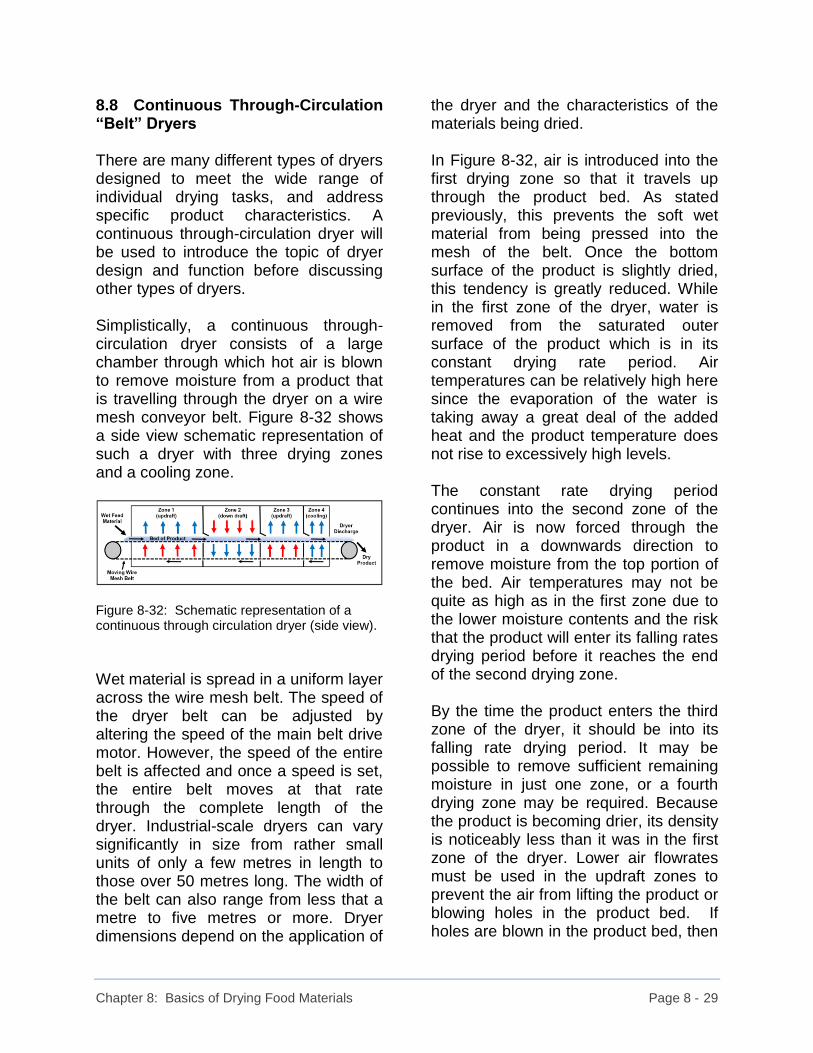
Chapter 8: Basics of Drying Food Materials Page 8 - 29
8.8 Continuous Through-Circulation “Belt” Dryers There are many different types of dryers designed to meet the wide range of individual drying tasks, and address specific product characteristics. A continuous through-circulation dryer will be used to introduce the topic of dryer design and function before discussing other types of dryers. Simplistically, a continuous through-circulation dryer consists of a large chamber through which hot air is blown to remove moisture from a product that is travelling through the dryer on a wire mesh conveyor belt. Figure 8-32 shows a side view schematic representation of such a dryer with three drying zones and a cooling zone.
Figure 8-32: Schematic representation of a continuous through circulation dryer (side view).
Wet material is spread in a uniform layer across the wire mesh belt. The speed of the dryer belt can be adjusted by altering the speed of the main belt drive motor. However, the speed of the entire belt is affected and once a speed is set, the entire belt moves at that rate through the complete length of the dryer. Industrial-scale dryers can vary significantly in size from rather small units of only a few metres in length to those over 50 metres long. The width of the belt can also range from less that a metre to five metres or more. Dryer dimensions depend on the application of
the dryer and the characteristics of the materials being dried. In Figure 8-32, air is introduced into the first drying zone so that it travels up through the product bed. As stated previously, this prevents the soft wet material from being pressed into the mesh of the belt. Once the bottom surface of the product is slightly dried, this tendency is greatly reduced. While in the first zone of the dryer, water is removed from the saturated outer surface of the product which is in its constant drying rate period. Air temperatures can be relatively high here since the evaporation of the water is taking away a great deal of the added heat and the product temperature does not rise to excessively high levels. The constant rate drying period continues into the second zone of the dryer. Air is now forced through the product in a downwards direction to remove moisture from the top portion of the bed. Air temperatures may not be quite as high as in the first zone due to the lower moisture contents and the risk that the product will enter its falling rates drying period before it reaches the end of the second drying zone. By the time the product enters the third zone of the dryer, it should be into its falling rate drying period. It may be possible to remove sufficient remaining moisture in just one zone, or a fourth drying zone may be required. Because the product is becoming drier, its density is noticeably less than it was in the first zone of the dryer. Lower air flowrates must be used in the updraft zones to prevent the air from lifting the product or blowing holes in the product bed. If holes are blown in the product bed, then

Chapter 8: Basics of Drying Food Materials Page 8 - 30
air may rush through these holes. Scorching of the product around the edges of the holes can result while leaving wet product in other areas of the bed. In addition to the lower air flowrates, lower temperatures are also used to prevent the material from being over-heated. As moisture diffuses from the inner portions of the material, product temperatures rise and thermal damage can result without due care being taken to keep such temperatures under control. If a fourth drying zone is needed, it may have downward air flow. The temperature of the air may be even lower than in the preceding third drying zone in order to prevent toasting, burning, or over-drying of the product. Some dryers may contain a final zone to cool the product with room-temperature air. This may also do a small amount of drying to bring the product into final conformance with the finished product moisture specifications. Cooling also prevents moisture uptake by the product when it leaves the dryer, as well as lowering the temperature of a starchy material to a point below its glass transition temperature. Once below its glass transition temperature, the product will be more rigid than it was in its softer amorphous form above its glass transition temperature. Air used to cool the product should have a low moisture content as reflected by a low relative humidity. If the relative humidity is high, the air can add moisture to the warm dry product. Retention times are controlled by the speed of the dryer belt and the length of the drying zone. It is very important to
understand the properties of the material being dried during the design stages of the dryer. Dryers are very large and costly. Poor dryer design will almost certainly result in poor dryer performance with the dryer being unable to deliver the desired product quality or uniform finished product moistures. The first zone is usually the longest zone in the dryer. As an example of how zone lengths may be varied to give appropriate retention times, consider a 30 metre (ca. 100 feet) long belt dryer. The first drying zone may be 12 metres long. It will have “updraft” air flow and be working to dry the product during its constant rate drying period The second zone, usually a downdraft zone, may be 9 metres long. It too may be working during the constant drying rate period and, perhaps, into the falling rate drying period. The third zone may be 6 metres long, and may be doing some gentle drying during the falling rate period. The final zone, for cooling may be only 3 metres long. Not only does it help to cool the product, but it may also finish off the drying during the last stages of the falling rate period. Delivering sufficient quantities of heated air to the dryer is important. Large fans are used to blow the air that has been heated by gas flames or steam tubes into the dryer zones. After the air enters the dryer zone chambers its flow is quite chaotic and tends to be non-uniform from one side of the zone to the other, and from one end of the zone to the other. In addition, the air flow patterns may be constantly changing. There are several different ways to produce a more uniform pattern of air distribution inside each dryer zone. One way is to install louvres, baffles, or deflectors. The
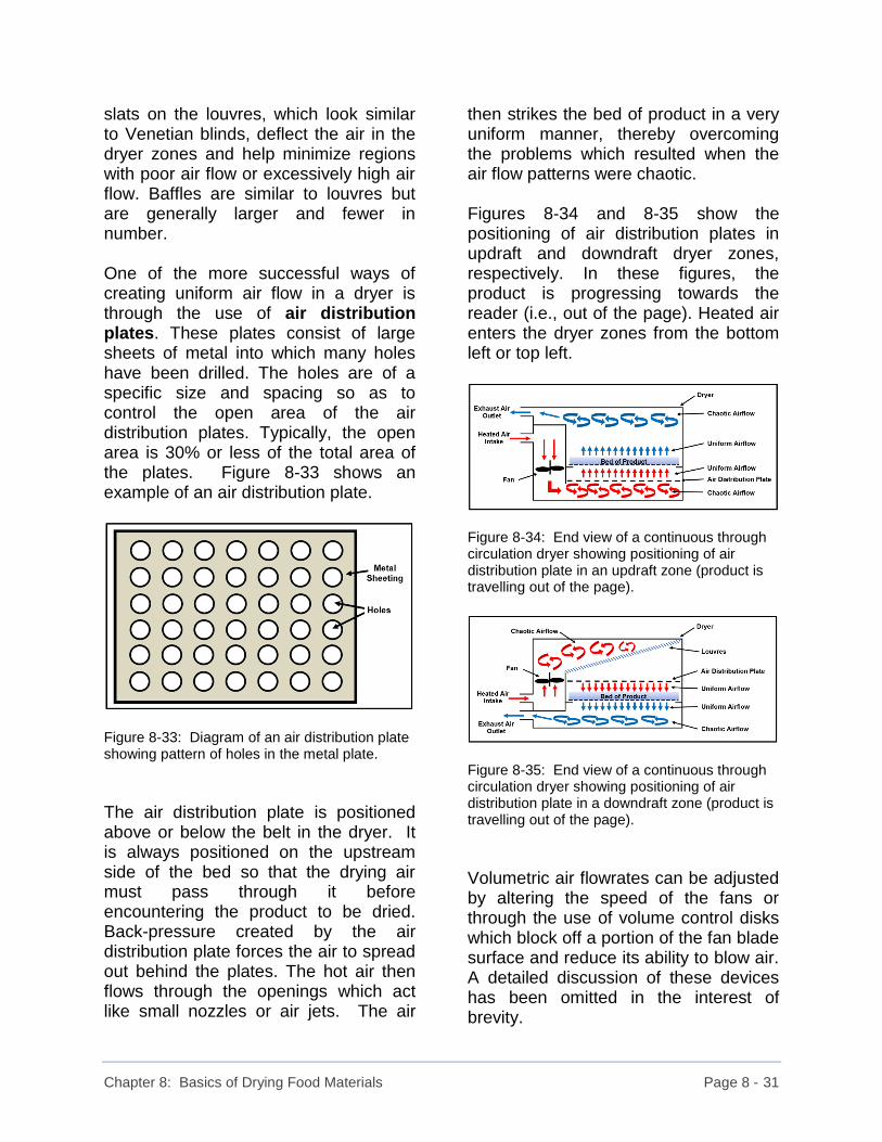
Chapter 8: Basics of Drying Food Materials Page 8 - 31
slats on the louvres, which look similar to Venetian blinds, deflect the air in the dryer zones and help minimize regions with poor air flow or excessively high air flow. Baffles are similar to louvres but are generally larger and fewer in number. One of the more successful ways of creating uniform air flow in a dryer is through the use of air distribution plates. These plates consist of large sheets of metal into which many holes have been drilled. The holes are of a specific size and spacing so as to control the open area of the air distribution plates. Typically, the open area is 30% or less of the total area of the plates. Figure 8-33 shows an example of an air distribution plate.
Figure 8-33: Diagram of an air distribution plate showing pattern of holes in the metal plate.
The air distribution plate is positioned above or below the belt in the dryer. It is always positioned on the upstream side of the bed so that the drying air must pass through it before encountering the product to be dried. Back-pressure created by the air distribution plate forces the air to spread out behind the plates. The hot air then flows through the openings which act like small nozzles or air jets. The air
then strikes the bed of product in a very uniform manner, thereby overcoming the problems which resulted when the air flow patterns were chaotic. Figures 8-34 and 8-35 show the positioning of air distribution plates in updraft and downdraft dryer zones, respectively. In these figures, the product is progressing towards the reader (i.e., out of the page). Heated air enters the dryer zones from the bottom left or top left.
Figure 8-34: End view of a continuous through circulation dryer showing positioning of air distribution plate in an updraft zone (product is travelling out of the page).
Figure 8-35: End view of a continuous through circulation dryer showing positioning of air distribution plate in a downdraft zone (product is travelling out of the page).
Volumetric air flowrates can be adjusted by altering the speed of the fans or through the use of volume control disks which block off a portion of the fan blade surface and reduce its ability to blow air. A detailed discussion of these devices has been omitted in the interest of brevity.
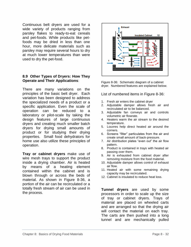
Chapter 8: Basics of Drying Food Materials Page 8 - 32
Continuous belt dryers are used for a wide variety of products ranging from parsley flakes to ready-to-eat cereals and pet-foods. While products like pet-foods may be dried in less than one hour, more delicate materials such as parsley may require several hours to dry at much lower temperatures than were used to dry the pet-food. 8.9 Other Types of Dryers: How They Operate and Their Applications: There are many variations on the principles of the basic belt dryer. Each variation has been designed to address the specialized needs of a product or a specific application. Even the scale of operation can be reduced to a laboratory or pilot-scale by taking the design features of large continuous dryers and creating much smaller batch dryers for drying small amounts of product or for studying their drying properties. Small food dehydrators for home use also utilize these principles of operation. Tray or cabinet dryers make use of wire mesh trays to support the product inside a drying chamber. Air is heated by means of a heating element contained within the cabinet and is blown through or across the beds of material. As shown in Figure 8-36, a portion of the air can be recirculated or a totally fresh stream of air can be used in the process.
Figure 8-36: Schematic diagram of a cabinet dryer. Numbered features are explained below.
List of numbered items in Figure 8-36: 1. Fresh air enters the cabinet dryer 2. Adjustable damper allows fresh air and
recirculated air to be balanced. 3. Adjustable fan conveys air and controls
volumetric air flowrate. 4. Heaters warm the air stream to the desired
temperature. 5. Louvres help direct heated air around the
corners. 6. Screens “filter” particulates from the air and
create small amount of back-pressure. 7. Air distribution plates “even out” the air flow
pattern. 8. Product is contained in trays with heated air
passing over them. 9. Air is exhausted from cabinet dryer after
removing moisture from the food material. 10. Adjustable damper allows control of exhaust
air flow. 11. Heated air with some remaining drying
capacity may be recirculated. 12. Cabinet is insulated to reduce heat loss.
Tunnel dryers are used by some processors in order to scale up the size of tray or cabinet dryers. Trays of material are placed on wheeled carts and are arranged so that the drying air will contact the material on each tray. The carts are then pushed into a long tunnel and are mechanically pulled
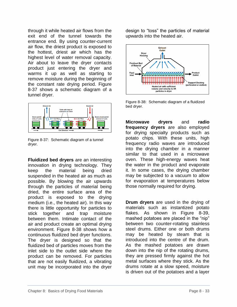
Chapter 8: Basics of Drying Food Materials Page 8 - 33
through it while heated air flows from the exit end of the tunnel towards the entrance end. By using counter-current air flow, the driest product is exposed to the hottest, driest air which has the highest level of water removal capacity. Air about to leave the dryer contacts product just entering the dryer and warms it up as well as starting to remove moisture during the beginning of the constant rate drying period. Figure 8-37 shows a schematic diagram of a tunnel dryer.
Figure 8-37: Schematic diagram of a tunnel dryer.
Fluidized bed dryers are an interesting innovation in drying technology. They keep the material being dried suspended in the heated air as much as possible. By blowing the air upwards through the particles of material being dried, the entire surface area of the product is exposed to the drying medium (i.e., the heated air). In this way there is little opportunity for particles to stick together and trap moisture between them. Intimate contact of the air and product create an optimal drying environment. Figure 8-38 shows how a continuous fluidized bed dryer functions. The dryer is designed so that the fluidized bed of particles moves from the inlet side to the outlet side where the product can be removed. For particles that are not easily fluidized, a vibrating unit may be incorporated into the dryer
design to “toss” the particles of material upwards into the heated air.
Figure 8-38: Schematic diagram of a fluidized bed dryer.
Microwave dryers and radio frequency dryers are also employed for drying specialty products such as potato chips. With these units, high frequency radio waves are introduced into the drying chamber in a manner similar to that used in a microwave oven. These high-energy waves heat the water in the product and evaporate it. In some cases, the drying chamber may be subjected to a vacuum to allow for evaporation at temperatures below those normally required for drying. Drum dryers are used in the drying of materials such as instantized potato flakes. As shown in Figure 8-39, mashed potatoes are placed in the “nip” between two counter-rotating stainless steel drums. Either one or both drums may be heated by steam that is introduced into the centre of the drum. As the mashed potatoes are drawn down into the nip of the rotating drums, they are pressed firmly against the hot metal surfaces where they stick. As the drums rotate at a slow speed, moisture is driven out of the potatoes and a layer

Chapter 8: Basics of Drying Food Materials Page 8 - 34
of dried potato flakes is left clinging to the drum. Just before the potatoes go over the top of the drum and back into the area where fresh mashed potatoes are being continuously added, a scraper blade, often called a “doctor blade”, scrapes the flakes off the drum and they fall into a hopper from which they are carried away for further processing.
Figure 8-39: Schematic diagram of a drum dryer.
Variations are available for drying different products with a drum dryer. However, we will not discuss them here. Spray dryers are often used in the pharmaceutical and crystal beverage industries to remove water from liquid solutions or slurries and create a powdered product. Solutions containing the product to be dried are sprayed into the upper portion of a tall drying tower in the form of tiny droplets. They are dispersed into a stream of heated air which is blowing into the top of the dryer to create a swirling pattern. As the droplets fall, moisture is evaporated into the air. The solid powdered material is collected at the bottom of the spray dryer and removed for further processing. Some of the powder particles may be so light that they are
carried out of the dryer in the air stream. These particles can be recovered from the exhaust air in a cyclone separator. Once separated from the air stream, the particles can be processed into larger granules or flakes etc. Figure 8-40 shows how a typical spray dryer operates.
Figure 8-40: Schematic diagram of a spray dryer system.
Figure 8-41 shows a pilot-scale spray dryer installation. The small conical device on the right is a cyclone separator to remove the dried powder from the air stream leaving the bottom of the spray dryer.
Figure 8-41: Photo of a spray dryer system.
Chapter 8: Basics of Drying Food Materials Page 8 - 35
8.10 Dryer Water Removal Capacity There are additional dryers available for many drying applications other than those listed above. It should be remembered that each material or product has its own characteristic drying behaviour. When establishing a drying process, care must be taken in selecting the proper dryer. It is frequently best to work with a reputable dryer supplier who can offer advice and may even be able to accommodate test runs on small-scale equipment to assist in the dryer design. Once the behaviour of a specific product is understood, design of a dryer can proceed. One of the first concerns will be the determination of the water removal capacity of the dryer. The basic function of a dryer is to remove moisture. Every dryer has a limit to how much water it can remove from a particular type of product in a given amount of time. This is its water removal capacity. First, it is necessary to determine how much finished product must be manufactured in a given amount of time. From this, the amount of water that must be removed in the drying process can be calculated. After the dryer is built and installed, there is little opportunity to change its water removal capacity. Some processors find that they have under-estimated the amount of product they must make, or markets have improved and sales may have increased so that they need to raise their production rates. They may attempt to add extra capacity to their dryers by increasing the size of the heaters or enhancing the volumetric air flowrates or
other similar method. However, success is usually quite limited because of the physical constraints of the existing dryer in meeting the time constraints of the constant and falling drying rate periods of the product. Consider the example of a drum dryer unit that is designed to remove a maximum of 1,000 kg of water per hour from mashed potatoes in the production of instant potato flakes. When trying to remove 900 kg of water per hour, the system will work quite well. However, in cases where additional mashed potatoes are required and the dryer is being “pushed” to remove 1,200 kg of water per hour, the results will most likely be disappointing. Dryers cannot be expected to perform at levels above their designed water removal capacity and still deliver a quality finished product. It should also be kept in mind that today’s drying needs may change and some flexibility concerning water removal capacities should be incorporated into the dryer design. As mentioned previously, it is often the case that as sales of a product expand, the need for more dryer throughput increases. Without the ability to remove additional water from a product no such expansion is possible and business opportunities may be missed.

Chapter 8: Basics of Drying Food Materials Page 8 - 36
8.11 Osmotic Dehydration Earlier in this chapter (in Section 8.3), we mentioned that salting has been a means of preserving foods for hundreds of years. Fish (e.g., cod) and various meats are examples of foods preserved in this manner. The mechanism by which moisture is withdrawn from the product is “osmosis”. Tissue or cells of fruits and vegetables contain moisture held within a semi-permeable membrane that makes up the cell wall. Under normal conditions, water flows through this membrane from the outside environment into the cell and waste products flow in the opposite direction. This is due to a concentration gradient or differential of dissolved compounds, such as sugars, between the liquid within the cell wall and outside the cell walls. We refer to these dissolved compounds as “solutes” because they are dissolved in the water, which we refer to as the “solvent”. A solution is made up of the liquid phase (i.e., the solvent) and the dissolved material (i.e., the solute). Typically, the concentration of solutes is higher within the cell than outside the cell. In order to equalize the concentration within the cell, water flows from the area of low solute concentration through the cell wall into the cell where the concentration of solutes is higher. If the concentration of a solute species such as sugar or salt is increased outside the cell to a level significantly above that within the cells, moisture will be drawn out of the cells. By exploiting the principle of osmosis in this manner,
water can be effectively removed from food tissue. Although the moisture content of the food cannot be reduced to low enough levels to preserve the food, osmotic dehydration can be combined with a final air-drying step to lower the moisture content and render the food safe for extended storage. In the salting of cod, the combination of osmotic dehydration and open-air drying creates a stable product with a significant shelf-life. The presence of the salt also renders the food safe from spoilage by most microorganisms which are unable to reproduce in high salt concentrations. In order to eat salted foods, they must be soaked in fresh water to remove the excess salt. Often, the water used for soaking must be changed several times to accomplish this and reduce the sodium levels. There is a quick little experiment that you can do to see how effective salt is at removing moisture from a food material. Cut a fresh firm carrot lengthwise into a number of strips. Place the carrot strips in a container and cover them with salt (Figure 8-42). After a few hours, the salt will start to clump and the carrot strips will become less firm to the point where they can be easily bent.
Figure 8-42: Strips of carrots have been covered in salt to illustrate moisture removal.
Processors have long been using concentrated sugar solutions (i.e., 50% to 60% by weight sucrose) at elevated temperatures (e.g., 50°C to 60°C) to remove moisture from sliced mangoes

Chapter 8: Basics of Drying Food Materials Page 8 - 37
and other fruits. The concentrated sugar solution draws moisture out of the fleshy portion of the mango. In the process, some sugar may go into the mango flesh and sweeten it even more than it is naturally sweetened. The partially dried mango slices can then be dried to the desired final moisture in a traditional forced air dryer. One of the problems using concentrated sugar solutions for osmotic dehydration is that you end up with large volumes of dilute sugar solutions. While it may be possible to partially re-concentrate the sugar solutions using membrane technology methods, there is still a problem with the volumes of syrup left from the process. A more recent approach to osmotic drying is to sprinkle dry, granulated sugar on the sliced material and allow it to draw moisture outwards. Figure 8-43 shows several mango slices in a plastic container. The weight of the mango slices was 80 grams.
Figure 8-43: Mango slices prior to the start of the osmotic dehydration process.
A layer of sugar was then sprinkled over these slices. The weight of sugar was equal to approximately half the weight of
the mango slices (i.e., about 40 grams). Figure 8-44 shows the mangoes coated with sugar soon after it was applied.
Figure 8-44: 80 grams of mango slices with approximately 40 grams of sugar (i.e., sucrose).
The container was covered and allowed to sit for 8 hours at room temperature (approximately 22°C). During this time, most of the sugar granules dissolved in the moisture drawn out of the mango flesh and formed a syrup as shown in Figure 8-45. There were still a few sugar crystals left undissolved in the bottom of the container.
Figure 8-45: Mango slices after 8 hours exposure to the sugar at room temperature.
After 24 hours, all traces of the sugar granules had disappeared. The slices of mango were removed from the sugar solution and rinsed briefly to remove the adhering sugar solution. After being blotted dry with a paper towel, the

Chapter 8: Basics of Drying Food Materials Page 8 - 38
samples were weighed. The 80 grams of mango slices originally present weighed 48 grams after the osmotic dehydration treatment. This indicated a weight loss of 32 grams due to the water removed by the sucrose crystals. Assuming an initial moisture content of 85% on a wet basis (5.67 grams of water per gram of dry solids), the final moisture content would be 75% on a wet basis (3.0 grams of water per gam of dry solids). While the loss of 10% moisture on a wet basis does not seem very substantial, the actual water removed by the sugar is 2.67 grams of water per gram of dry solids. This is slightly over half of the initial water present in the sample. The partially dried mango slices are shown in Figure 8-46.
Figure 8-46: Partially dried mango slices after osmotic dehydration step.
The partially dehydrated slices of mango can be removed from the syrup and dried in a conventional forced air dryer to reduce the water content to the desired level. There may be alternate uses for the syrup to reduce its waste. The dried mangoes may be dusted in fine sugar before packaging. This will help prevent them from becoming stuck together, may help take up any excess
moisture in the package, and may increase the overall sweetness of the dried mangoes. Often, osmotically dehydrated mango slices have a lighter, more appealing colour than air-dried mango slices. Figure 8-47 shows an air-dried sample on the left and an osmotically dehydrated mango sample on the right. The air-dried sample may have been dried at an excessively high temperature or over-dried to get its rather dark colour. Not all air-dried samples are this dark.
Figure 8-47: Samples of commercially available dried mango slices with an air-dried sample on the left, and an osmotically dehydrated sample on the right.
The syrup that is a by-product from the osmotic dehydration process is not only quite sweet, but it also has a mango flavour to it. It may have potential for use in beverages where sugar must be added and the mango flavour is not objectionable.

Chapter 8: Basics of Drying Food Materials Page 8 - 39
8.12 Sample Calculations Sample Question 8-4: How much water must be removed from 600 kg of apricot slices (85% moisture) to prepare dried apricots with a final moisture content of 18%? What will be the weight of the final product? Solution: First, it should be pointed out that it is not permissible just take the difference between the initial moisture and final moisture (i.e., 85% - 18%) and multiply that value by the initial weight of the material. This is a very common error that fails to recognize the fact that wet basis moistures cannot be added or subtracted since they are not linear (see Figures 8-6 and 8-7). Figure 8-48 shows the drying process using photos of the fresh and dried apricots.
Figure 8-48: Pictorial representation of the apricot drying process.
Start by determining the amount of water and solids present in the 600 kg of apricots. If 85% of the weight is water, then the remaining 15% will be solids. Weight of water in apricots = 600 kg x 0.85 = 510 kg
Weight of solids in apricots = 600 kg - 510 kg of water = 90 kg or: Weight of solids = 600 kg x 0.15 = 90 kg Since the weight of the final product is not known, let that weight be X kg. Of the final weight 18% is water, so 82% must be solids. No solids were mentioned as being lost in the drying process, which means that the weight of the solids in the final product should be the same as the weight of the solids in the initial apricots. Therefore, the following is true: Weight of dry solids in final product = 90 kg This is 82% of the final product weight. 0.82 X = 90 kg This implies: X = 90 kg = 109.76 kg 0.82 If the total weight of the final product is 109.76 kg and 90 kg of this are solids, then 19.76 kg must be water (i.e., 109.76 kg - 90 kg solids = 19.76 kg water). Amount of water to be removed = water at start - water in final product = 510 kg - 19.76 kg = 490.24 kg Therefore, approximately 490 kg of water must be removed and approximately 110 kg of final product are obtained from the drying process.

Chapter 8: Basics of Drying Food Materials Page 8 - 40
Sample Question 8-5: What weight of fresh apple slices (84% wet basis moisture) is required to produce 150 kg of dried apples with a moisture content of 10%? Solution: It may be helpful to start with a simple diagram to organize the information. Figure 8-49 gives a pictorial representation of the problem.
Figure 8-49: Pictorial representation of the apple slice drying process.
In order to begin this solution, the weight of water and solids present in the final product must be determined. Then a way of relating this information back to the weight of the starting material must be established. Weight of water in dried apples = 150 kg x 0.10 = 15.0 kg Weight of solids in dried apples = 150 kg x 0.90 = 135.0 kg or: Weight of solids in dried apples = 150 kg – 15.0 kg water = 135.0 kg
Since no losses of solids are mentioned during the drying process, it would be reasonable to assume that the weight of solids present in the apples initially would be equal to the weight of solids in the final product. Let the weight of the starting material be X kg of which 135.0 kg are solids and the remainder is water. Since the water content is 84%, the solids content of the fresh apples will be 16% (i.e., 100% - % water). Weight of solids in starting material = X kg x 0.16 = 135.0 kg Solving for X: Weight of starting material = X kg = 135.0 kg = 843.75 kg 0.16 Therefore, the weight of fresh apple slices required would be 843.75 kg. Therefore, the initial weight of fresh apple slices would be approximately 844 kg.

Chapter 8: Basics of Drying Food Materials Page 8 - 41
Sample Question 8-6: Calculate the weight of dry solids lost in a process designed to dry fresh parsley (85.0% moisture) to dried powder at 8.0% wet basis moisture. The processor started with 350 kg of fresh parsley and ended up with 54.5 kg of powdered parsley. Calculate how much water was removed in the process as well. Solution: Figure 8-50 shows what is happening in this process. Some parsley flakes are lost, possibly due to falling through the mesh screen in the dryer or having small pieces being carried away in the exhaust air.
Figure 8-50: Pictorial representation of the parsley drying process.
As usual, it is best to calculate the amount of solids and water present in the materials that you have been given. Weight of water in fresh parsley = 350 kg x 0.85 = 297.5 kg Weight of solids in fresh parsley = 52.5 kg Weight of water in dried parsley = 54.5 kg x 0.08 = 4.36 kg
Weight of solids in dried parsley = 54.5 kg x 0.92 = 50.14 kg Weight of solids lost in process = weight of solids - weight of solids at start at end = 52.5 kg – 50.14 kg = 2.36 kg Weight of water removed = weight of water - weight of water at start at end = 297.5 kg – 4.36 kg = 293.14 kg Therefore 2.36 kg of dried parsley solids are lost in the process and 293.14 kg of water are removed from the fresh parsley to get the 54.5 kg of dried product.

Chapter 8: Basics of Drying Food Materials Page 8 - 42
8.13 Practice Problems 1. Calculate the dry basis moisture
content of the following materials:
a. Honey at 17% wet basis moisture (Ans. 0.20 g water / g dry solids)
b. Fresh beef at 88% moisture (Ans. 7.33 g water / g dry solids)
c. Fresh perch (fish) at 81% moisture
(Ans. 4.26 g water / g dry solids)
d. Blueberries at 82% moisture (Ans. 4.56 g water / g dry solids)
e. A mixture of 12 kg sugar with
12% moisture and 10 kg water (Ans. 1.08 kg water / kg dry solids) f. 65° Brix apple juice concentrate (Ans. 0.54 g water / g dry solids) 2. Determine the wet basis moisture of
the following:
a. Squash containing 15.67 g water per g dry solids (Ans. 94%)
b. 150 kg of black raspberries
containing 121.5 kg water (Ans. 81%)
c. 95 kg peach slice containing 10.5
kg dry solids (Ans. 88.9%) d. A mixture of 12 kg sugar with
12% moisture and 10 kg water (Ans. 52.0%)
e. 55° Brix apple juice concentrate
(Ans. 45%)
3. Assuming skim milk contains 9.0% solids, how much water must be removed from 1,500 litres of skim milk (specific gravity = 1.035) to obtain skim milk powder with a moisture content of 5% by weight? How much skim milk powder will be obtained? (Ans. 1,405 kg of water must be removed and 147 kg of skim milk powder will be obtained)
4. How much water must be removed
from 1,000 litres of fresh squeezed apple juice with 10.2% solids (Density = 1.04 kg/litre) to prepare a concentrate with a solids concentration of 65° Brix? How much concentrate is obtained from this process? (Ans. 876.8 kg of water must be removed and 163.2 kg of concentrate will be obtained)
Note: Brix is used to define the
concentration of sugar in solution. One degree Brix (i.e., 1°Brix) is equal to one percent sugar by weight. The “degrees” have nothing to do with temperature.
5. If 265 kg of water is removed from
500 kg of sweet peppers (92% moisture), what would be the final product moisture? (Ans. 83.0%).
Dried peppers should have a final
moisture content of 12% (wet basis). How much water should actually be removed from the 500 kg of peppers with 92% moisture to reach this target value? (Ans. 454.6 kg of water should be removed)

Chapter 8: Basics of Drying Food Materials Page 8 - 43
8.14 Specialized Drying Calculations This chapter has attempted to provide insight into the basics of food drying. Information presented here should be sufficient to allow you, as a small-scale processor or entrepreneur, to understand the basic principles of drying and apply them to various fruits and vegetables. Of course, there is a great deal more that can be discussed with regard to drying food products. We could look into gathering data from drying trials and evaluating the kinetics of the drying process. This rate of water removal with respect to time can be quite useful in modelling drying processes. We could also examine methods of comparison of drying rates for different drying conditions and a variety of other more complicated mathematical treatments. It is my personal feeling that moving into the complexities of drying rates and mathematical modelling of processes is not necessary for what most people are actually attempting to do when they dry fruits and vegetables. Inclusion of such material would unnecessarily complicate our overview of the topic. Should you wish to move deeper into the study of food drying, there are numerous sources available, either in the form of printed textbooks designed for university level studies, or through on-line sources geared to a similar audience. In 2014, I prepared “An Introduction to the Dehydration and Drying of Fruits and Vegetables” which is an e-book
available free of charge through several on-line sources. There are also video presentations that accompany this 300-page drying manual. The e-book itself consists of two sections. The first part deals with the principles of drying and goes more deeply into things than this chapter has done. The second part examines the drying kinetics of approximately twenty-five fruits and vegetables of particular interest to those in the Caribbean area where I was conducting training activities at the time. Figure 8-51 shows the cover of this e-book. Its ISBN is: 978-0-88955-621-8.
Figure 8-51: Cover of e-book “An Introduction to the Dehydration and Drying of Fruits and Vegetables”.

Chapter 8: Basics of Drying Food Materials Page 8 - 44
8-15 References ASHRAE, Selected data from “The 1986 ASHRAE Handbook – Refrigeration”. American Society of Heating, Refrigerating, and Air Conditioning Engineers, 1986 Barbosa-Canovas, Gustavo V., and Humberto Vega-Mercado. “Dehydration of Foods”. Springer Science and Business Media, New York, 1996. Mercer, D.G., personal data.
Mercer, Donald G., “An Introduction to the Dehydration and Drying of Fruits and Vegetables”, 2014. E-book, available on-line in two parts at iufost.org/iufostftp/Drying-Part1.pdf and iufost.org/iufostftp/Drying-Part2.pdf Accessed April 2018.

Chapter 9: Chilling and Freezing Page 9 - 1
9. Chilling and Freezing 9.1 Introduction In this chapter we will provide details about various aspects of chilling and freezing processes and their effects on food products. Both of these techniques are indispensable in preserving food quality and helping to extend the shelf-life of perishable and semi-perishable food materials. 9.2 What is “Chilling”? There is really no precise definition for the “chilling” of foods. Basically, we can look at it as simply reducing the temperature to any point below ambient conditions. However, there is a tendency to think of chilling as reducing the temperature of a product to 15⁰C, or
less, while not allowing it to go below the freezing point of the product, or of pure water. Within this temperature range, we have what is generally considered as being “refrigeration temperature” at 4⁰C.
Mild chilling may be done at a storage temperature of below 10⁰C. The 15⁰C
temperature mentioned previously is recognized by some as being mild chilling. It should be noted that the presence of sugars and other compounds in fruits and vegetables may reduce their freezing points to slightly below that of pure water (i.e., 0⁰C).
In some cases, chilling may be extended below 0⁰C if sufficient dissolved solids
are present to prevent the onset of
freezing of water present in the product. These chilled temperatures may be as low as -4⁰C, but they are dependent on
the actual food being considered. For example purposes, we can look at the freezing point of apples which is -1.1⁰C.
Green peas freeze at about -0.6⁰C, and
leafy greens freeze at about -0.3⁰C.
Therefore, to simplify matters, we will look at “chilling” as the reduction of the temperature of a product to a point between the freezing point of water (i.e., 0⁰ C) and 10⁰C. Some reference
sources may use 15°C as the upper limit of the chilled temperature range. In the overall scheme of things, this is not an issue. 9.3 How Does Chilling Differ from Freezing? Since chilling is done at temperatures above the freezing point of water, there is no opportunity for any water present in the food to actually freeze. This means that any water present in the food has not undergone a change in state from its liquid form to the crystalline solid form we call “ice”. Because the water is present as a liquid in chilled foods, there is no significant difference between the food in its chilled state and the way it was prior to chilling. You may want to compare this to what happens when foods are dried to remove moisture and thereby reduce spoilage. Dried foods tend to be significantly different from their fresh counterpart than refrigerated foods are from their un-chilled counterpart.

Chapter 9: Chilling and Freezing Page 9 - 2
With chilling, there are no drastic changes in the food itself. This may lead us to consider “chilling” as being a method of handling food, as opposed to a method of processing it. For those who are familiar with “freezing” as a method of processing and preserving food, you will be familiar with the formation of ice crystals within the product, and the effects that they can have on the overall food quality. In chilling, there are no ice crystals to rupture membranes of the cells within the food. Nor is there the problem of ice crystal growth that robs the cells of moisture causing them to shrink and create a phenomenon called “freezer burn”. 9.4 Why Do We Chill Food? The purpose of chilling various foods is to extend their usable shelf-life. “Shelf-life” is a term we use to describe how long a product will keep its level of acceptable quality and be suitable for consumption. Products with a short shelf-life will need to be consumed very soon after they are harvested, or else they will spoil and be unsuitable for eating. This would be true for leafy greens such as lettuce, or for products such as fresh mushrooms. Grains, such as wheat or rice, have a much longer shelf-life and will retain their quality long after they are harvested. For some products, the duration of the extra shelf-life may be only a few days compared to the same product stored at room temperature. However, these few extra days can be important to food distributors who will experience less waste, or will be able to expand their
distribution network if chilled storage conditions are employed. For other products, the storage life may be extended by a week or more. This is the case with many dairy products such as milk or yoghurts, etc. The exact time frame is dependent upon the material and the conditions within the chilled storage area. As we will see, there is more to chilling than simply lowering the temperature. Chilling works by slowing the rate of chemical reactions which lead to deterioration of foods. It also slows the growth of microorganisms which lead to spoilage. Some fruits and vegetables contain enzymes which are biological catalysts that increase the rate of degradation at the molecular or cellular level through such things as changes in colour as seen when white cauliflower turns brown or black with time. By slowing these degradative processes, quality is maintained for longer than it normally would be if the foods were left at room temperature. It should be mentioned that not all foods need to be refrigerated and that some should not be subjected to reduced temperatures since their quality may suffer. An example of this is bread, which we will examine later. Perishable and semi-perishable foods are of particular interest when it comes to chilling as a means of extending shelf-life and maintaining quality. While shelf-life extension is the main reason for chilling foods, it is not the only reason.

Chapter 9: Chilling and Freezing Page 9 - 3
Chilling may be required to create special conditions to bring about desired changes in a food process. An example of this would be in the churning of butter or the making of margarine where it is necessary to produce an emulsion of water droplets in an oil. Chilling also helps prevent the loss of flavours and aromatic compounds from foods by reducing the rate at which they evaporate and leave the food. You may have noticed that if something is cold and is heated that it will give off more aroma. While this may be pleasant to the consumer, we do not want to lose these “volatile” components before the product is being used. 9.5 How Do We Chill Food? Fruits, vegetables, meats, and other foods can be chilled by exposing them to cold air in an enclosed space. Typically, the air is cooled by passing it over refrigeration coils through which a cold liquid or gaseous refrigerant is passing. It is important to have as much contact as possible between the cold air and the surface of the material being chilled. A sufficient air velocity is also required to sweep away any stagnant air along the surface which can form a barrier to the effective transfer of heat from the warm food to the cold air.
9.6 Perishability
There are three general classifications under which we can put most foods. These relate to how fast they deteriorate under various conditions of storage. Perishable foods tend to spoil quite rapidly at room temperature and will maintain their quality for about 2 to 30 days if stored under refrigerated conditions of 0⁰C to 4⁰C. Foods
included in this category are: fluid milk products, fresh meat, fish, poultry, fresh fruits and vegetables, fruit and vegetable juices, and various bakery items as well as some processed dairy products (Figure 9-1).
Figure 9-1: Fish, poultry, fresh fruit, and fresh vegetables are perishable products.
Semi-perishable foods do not spoil as rapidly as perishable foods, as their name implies. It is not unreasonable to expect them to have a shelf-life of 30 to 90 days when stored under proper conditions. Such conditions often involve being chilled (or refrigerated) at temperatures from 0⁰C to 4⁰C. It may
also be necessary to process foods by methods such as pasteurization, pickling, or smoking to change them from being perishable to semi-perishable. The use of salt, sugar, and
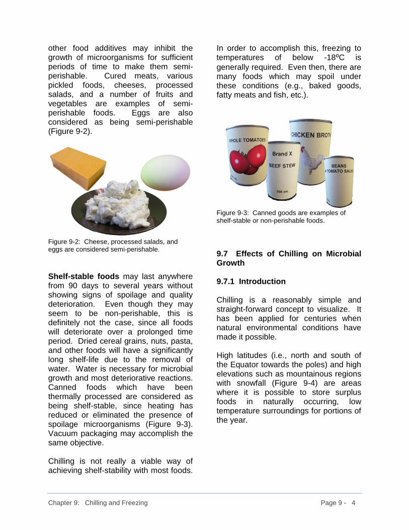
Chapter 9: Chilling and Freezing Page 9 - 4
other food additives may inhibit the growth of microorganisms for sufficient periods of time to make them semi-perishable. Cured meats, various pickled foods, cheeses, processed salads, and a number of fruits and vegetables are examples of semi-perishable foods. Eggs are also considered as being semi-perishable (Figure 9-2).
Figure 9-2: Cheese, processed salads, and eggs are considered semi-perishable.
Shelf-stable foods may last anywhere from 90 days to several years without showing signs of spoilage and quality deterioration. Even though they may seem to be non-perishable, this is definitely not the case, since all foods will deteriorate over a prolonged time period. Dried cereal grains, nuts, pasta, and other foods will have a significantly long shelf-life due to the removal of water. Water is necessary for microbial growth and most deteriorative reactions. Canned foods which have been thermally processed are considered as being shelf-stable, since heating has reduced or eliminated the presence of spoilage microorganisms (Figure 9-3). Vacuum packaging may accomplish the same objective. Chilling is not really a viable way of achieving shelf-stability with most foods.
In order to accomplish this, freezing to temperatures of below -18⁰C is
generally required. Even then, there are many foods which may spoil under these conditions (e.g., baked goods, fatty meats and fish, etc.).
Figure 9-3: Canned goods are examples of shelf-stable or non-perishable foods.
9.7 Effects of Chilling on Microbial Growth 9.7.1 Introduction Chilling is a reasonably simple and straight-forward concept to visualize. It has been applied for centuries when natural environmental conditions have made it possible. High latitudes (i.e., north and south of the Equator towards the poles) and high elevations such as mountainous regions with snowfall (Figure 9-4) are areas where it is possible to store surplus foods in naturally occurring, low temperature surroundings for portions of the year.

Chapter 9: Chilling and Freezing Page 9 - 5
Figure 9-4: High elevations have offered natural chilling and freezing since pre-historic times.
Fortunately, scientific developments have made it possible to create chilled storage conditions using modern refrigeration techniques designed for various applications. Refrigeration has now brought the ability to chill foods to all areas of the world where sufficient power is available to operate these devices.
9.7.2 Storage Temperatures Figure 9-5 shows a thermometer representing various temperatures and ranges typically encountered in food processing and handling plus several other important reference temperatures. Normal human body temperatures tend to be around 37⁰C. This also happens
to be the temperature at which many microorganisms grow best. 20⁰C or slightly higher is frequently
considered as being “ambient” temperature or the naturally occurring temperature in the environment or in the food processing area. The freezing point of pure water (i.e., 0⁰C) is also included in Figure 9-5 as
both a reference temperature, and what we are regarding as the lower end of the chilled temperature range. As seen in this figure, there is a range of chilled temperatures progressing from mild chilling from 10⁰C down to 4⁰C.
Then, we get into the refrigerated temperature range of 4⁰C down to 0⁰C.
After this, there is a lower chilled temperature range which goes to -4⁰C
for products that have a lower freezing point than that of pure water. Below -4⁰C, we see that the product
begins to freeze in a series of ranges from partial freezing (-5⁰C down to -8⁰C)
to totally frozen below -10⁰C. When
subjected to temperatures below -18⁰C,
the material is considered to be in a deep-frozen storage state.

Chapter 9: Chilling and Freezing Page 9 - 6
Figure 9-5: Temperature ranges encountered during food processing and handling. Based on various Internet and published sources.
9.7.3 Temperature Limits for Growth Now that we have examined the temperatures and ranges for chilling and freezing, let’s have a look at the temperatures which are at the lower end of the growth range for a number of food-borne microorganisms that cause spoilage and illnesses. These are shown in Figure 9-6. Most microorganisms tend to grow well at ambient to physiological temperatures which are in the range of 20⁰C to 37⁰C.
However, they can also grow above and below this range. For this reason, the temperature range from 10⁰C to 45⁰C is
often referred to as the “Danger Zone”. When food products are within this temperature range they are highly susceptible to microbial growth.
Figure 9-6: Lower temperatures for the growth of various microorganisms. Based on various Internet and published sources.
It is rather surprising to find in the literature (Hazeleger et al. 1998) that Campylobacter species do not usually grow below a temperature of about 32⁰C. This should not lull you into a
false sense of security, however. Just because ambient temperatures are too low to support the growth of a microorganism, that does not mean that it is not still present in a dormant state. Once the temperature increases to a value above its lower growth limit, the microorganism may begin to grow once again. This is what often happens in the case of chicken which has been chilled but is then improperly cooked. When the chicken is eaten, the dormant Campylobacter cells find themselves in a person’s digestive tract at 37⁰C where
they grow and may cause a serious sickness.

Chapter 9: Chilling and Freezing Page 9 - 7
Clostridium botulinum is the microorganism of interest when dealing with vegetables for canning etc. The rate of growth of most pathogens tends to decrease substantially below 10°C. In contrast, some strains of C. botulinum can grow to temperatures as low as 3°C which is well within the range of chilled temperatures and slightly below the commonly used refrigeration temperature of 4°C. There are other microorganisms which may also grow under chilled conditions, as shown in Figure 9-6. Continuing to look at Figure 9-6, we can see that there are even microorganisms which are capable of growth at or below the freezing point of water. Not only does this show us the adaptability of microorganisms in being able to grow under difficult conditions, but it tells us that chilling alone is not sufficient to protect us from microbial growth in food products. The important message to take from all this is that we absolutely must use chilling in conjunction with other approaches to maintain safety and quality in the foods we eat. Most important among these is ensuring cleanliness at all steps of the food chain.
9.7.4 Phases of Growth We have already stated that lower temperatures slow the growth rate of microorganisms. Now, we will take a look at this in somewhat more detail. Those who have taken a course in microbiology may be familiar with the typical patterns exhibited by yeasts and bacteria etc. as they grow under ideal conditions in a fermentation process, or simply in food that is left out at room temperature. Figure 9-7 shows the growth behaviour of microorganisms when they are at suitably warm temperature with an adequate supply of nutrients. This is the red curve (i.e., the upper curve in Figure 9-7).
Figure 9-7: Phases of growth of microorganisms under ideal conditions (red curve) and at chilled temperatures (blue curve).
When microorganisms are first introduced into their new environment, it takes them a period of time to adjust to their new surroundings. This is when they begin to produce enzymes to break down starches if they find themselves faced with starch as a food supply or “substrate”. As a result, there is only a

Chapter 9: Chilling and Freezing Page 9 - 8
slight change in the actual number of microorganisms present since there is little or no growth during this “lag stage”. Once the microorganisms have adjusted to their new environment, they begin to increase in number by utilizing the available nutrients. The microbial cells reproduce by such mechanisms as cell division, or budding in the case of yeasts. The rapid, continuous doubling produces an exponential or logarithmic growth period, which is referred to as the logarithmic, or “log phase”. Notice how steep the red growth curve is during the “log phase” in Figure 9-7. Eventually, the microbial population will reach a point where it has consumed most of the available nutrients that are present. Growth will begin to slow and the cell population will level off as we reach the “stationary phase” of the growth pattern. In some cases, the stationary phase may begin due to the production of by-products formed by the microbial cells as they grow. These by-products, such as alcohol, may inhibit further growth once they reach a threshold concentration. Sometimes, during the stationary phase, the microorganisms may detect the presence of another substrate which was originally less preferable than the initial substrate that it choose upon which to grow. In this case, there may be a brief delay while the microorganism goes through a second lag phase. There can then be a renewed period of growth in this “diauxic growth” process. There may also be a period of death for some of the microorganisms. The dead microorganisms can serve as a food source for the other dormant microbes in their stationary phase, which will then
show a brief period of renewed growth and reproduction until this substrate source is depleted. If everything in the fermentation process described by the red curve in Figure 9-7 is kept constant, except for the temperature which is being lowered to below 10°C, we will see a pronounced change in the growth pattern of the microorganism. This is shown by the blue curve in Figure 9-7. The initial population of cells will start out as being identical to the more “ideal” fermentation at the higher temperature. As the “lag phase” begins, the cells are slower to adjust to their new environment due to the reduced temperature. As a result, the lag phase lasts significantly longer under chilled conditions than it did when the system was warmer. Once the microorganisms begin to pull out of the lag phase and enter into the logarithmic or “log” phase, their overall rate of growth is still much slower than it was at higher temperatures. One of the objectives of refrigeration is to maintain storage conditions at an appropriately low temperature. These low temperatures will help keep any microorganisms present in the food product in their “lag phase”, and prevent them from entering their “log phase” of growth. While this may not always be possible, lowering the temperature will reduce the rate of growth in the event that the microbial cells do adjust to their new surroundings and begin their log phase of growth.

Chapter 9: Chilling and Freezing Page 9 - 9
9.8 Enzyme Activity in Stored Foods Enzymes are biologically active protein molecules produced by the cells of plants and animals to carry out some very specialized functions. These functions generally relate to promoting or “catalyzing” various biological reactions. In the brewing process, yeast cells produce enzymes capable of breaking down starches into smaller components (i.e., sugars) so that they can be used as nutrients. Without these amylase enzymes, the large starch molecules would be unusable by the yeast cells. Enzymes that are present in the cells of fruits and vegetables can speed the spoilage process. Once again, we will use the somewhat over-worked example of the enzyme polyphenol oxidase which is present in such plants as cauliflower. When selecting cauliflower for eating, we try to choose ones with white florets, since they are fresh and of high quality. If the cauliflower is allowed to stand at room temperature for an extended period of time, the florets will begin to turn from white to light brown and then darken as time goes on. Ultimately, the florets will become dark brown, purple, or black in colour. The reason for this is the reaction between the polyphenol oxidase and various phenolic compounds in the plant cells which change colour when they are reacted with oxygen. In Figure 9-8, we see a fresh cauliflower having creamy white florets.
Figure 9-8: Fresh cauliflower.
After remaining at room temperature for a number of days, we can see the change in colour as shown in Figure 9-9.
Figure 9-9: Cauliflower after sitting at room temperature for several days.
When fruits and vegetables are going to be frozen, they are usually “blanched” by soaking them in boiling hot water for approximately two to three minutes. This severe temperature treatment deactivates the enzymes and essentially eliminates the problems of “enzymatic browning”, as it is called. While blanching is possible when foods are being processed for longer term storage, we do not want to do anything

Chapter 9: Chilling and Freezing Page 9 - 10
of this nature to foods which are intended to be consumed in their fresh state. Since enzymatic reactions are actually chemical reactions involving biological catalysts, we can slow their rates by chilling. Using the approach that reducing the storage temperature by 10 C⁰ will reduce the deterioration
rate by one-half, we can see the obvious advantages to chilling many fruits and vegetables. In a Chapter 6, we showed how naturally occurring peroxidase enzymes in radishes and turnips react with hydrogen peroxide to form oxygen and water. The oxygen gas was given off as small bubbles that collected around the material. We can use this simple example to demonstrate the effect of temperature on the rate at which an enzymatic reaction proceeds. In Figure 9-10, we see the oxygen bubbles that have collected around some slices of carrot. The reaction was taking place at room temperature (about 22°C), and the photograph was captured from a video 30 seconds after the peroxide solution was poured onto the carrot slices.
Figure 9-10: Carrot slices in 3% hydrogen peroxide solution at 22°C (time = 30 seconds).
This test was repeated using hydrogen peroxide solution and a fresh set of carrot slices chilled to approximately 6°C. The plate was also chilled to keep the temperature as low as possible. 30 seconds after the cold hydrogen peroxide solution was poured over these chilled carrot slices, the photograph shown in Figure 9-11 was captured from a video of the test.
Figure 9-11: Carrot slices in 3% hydrogen peroxide solution at 6°C (time = 30 seconds).
A visual comparison of Figures 9-10 and 9-11 clearly illustrates that there are appreciably more oxygen bubbles released by the peroxidase reaction at the higher temperature than at the lower temperature. This visually supports the claim that lowering the temperature of a product can reduce the rate at which enzymatic reactions take place.
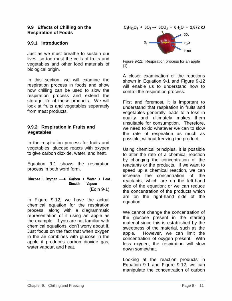
Chapter 9: Chilling and Freezing Page 9 - 11
9.9 Effects of Chilling on the Respiration of Foods 9.9.1 Introduction Just as we must breathe to sustain our lives, so too must the cells of fruits and vegetables and other food materials of biological origin. In this section, we will examine the respiration process in foods and show how chilling can be used to slow the respiration process and extend the storage life of these products. We will look at fruits and vegetables separately from meat products. 9.9.2 Respiration in Fruits and Vegetables In the respiration process for fruits and vegetables, glucose reacts with oxygen to give carbon dioxide, water, and heat. Equation 9-1 shows the respiration process in both word form.
(Eq’n 9-1) In Figure 9-12, we have the actual chemical equation for the respiration process, along with a diagrammatic representation of it using an apple as the example. If you are not familiar with chemical equations, don’t worry about it. Just focus on the fact that when oxygen in the air combines with glucose in the apple it produces carbon dioxide gas, water vapour, and heat.
Figure 9-12: Respiration process for an apple (1). A closer examination of the reactions shown in Equation 9-1 and Figure 9-12 will enable us to understand how to control the respiration process. First and foremost, it is important to understand that respiration in fruits and vegetables generally leads to a loss in quality and ultimately makes them unsuitable for consumption. Therefore, we need to do whatever we can to slow the rate of respiration as much as possible, without freezing the product. Using chemical principles, it is possible to alter the rate of a chemical reaction by changing the concentration of the reactants or the products. If we want to speed up a chemical reaction, we can increase the concentration of the reactants, which are on the left-hand side of the equation; or we can reduce the concentration of the products which are on the right-hand side of the equation. We cannot change the concentration of the glucose present in the starting material since this is established by the sweetness of the material, such as the apple. However, we can limit the concentration of oxygen present. With less oxygen, the respiration will slow down somewhat. Looking at the reaction products in Equation 9-1 and Figure 9-12, we can manipulate the concentration of carbon

Chapter 9: Chilling and Freezing Page 9 - 12
dioxide and water vapour in the enclosed storage space as well as the temperature of the storage environment. Technically speaking, if the temperature is allowed to increase, it should lower the rate of respiration based on these equations. However, we know that increasing the temperature will increase the rate of other reactions which are occurring, so overall, it is better to cool the storage area rather than have it warm up. It should be possible to allow the moisture content of the storage area to increase to slow the respiration rate. Unfortunately, if the moisture content of the air rises to an excessive level, conditions will become favourable for the growth of molds and other undesirable microorganisms. This leaves increasing the concentration of carbon dioxide as a potential way of lowering the rate of respiration. In practice, this is actually one of the things that is commonly done in the storage of such things as apples. By increasing the concentration of carbon dioxide to about 3.5% in the storage areas and reducing the temperature to the lower end of the chilled temperature range, apples may be successfully stored for several months while still retaining a relatively high quality. The first indications that quality is beginning to deteriorate is the development of small brown marks in the fleshy portion of the apple, followed by a softening of its texture. 9.9.3 Controlled Atmosphere Packaging
As discussed above, the combination of chilling plus altering or controlling the atmosphere in which the material is being held can enhance its storage life appreciably. This controlled atmosphere packaging approach is used for a variety of products, especially leafy vegetables like lettuce and spinach etc. which are used for salads (see Figure 9-13). Often, the leaves are rinsed in a chlorine solution to reduce their microbial load and then washed thoroughly to remove any residual chlorine before packaging. The leaves are placed in specially designed “plastic” bags which allow the transfer of gases between the contents of the bags and the outside air. By having pores or openings in the plastic that control the exchange of gases within certain limits, it is possible to have the desired balance of carbon dioxide and oxygen to maintain a low respiration rate while the bags are held under chilled storage conditions in the supermarket.
Figure 9-13: Salad greens in a controlled atmosphere package.
9.9.4 Respiration Rates of Various Fruits and Vegetables

Chapter 9: Chilling and Freezing Page 9 - 13
Respiration rates vary with the particular fruit or vegetable and may be classed as ranging from very low to very high. Even after harvesting, produce continues to respire. Respiration will have an impact on the quality and chemical composition of the produce due to the consumption of carbohydrates (i.e., sugars) as a source of energy that is released in the respiration process. The respiration rates of the same fruits or vegetables will also vary depending on the form in which is present. For example, dried apple slices will not have the same respiration rate as those from a fresh apple (Figure 9-14). As one would expect, the respiration rate of the apple cells with almost all of their moisture removed should be extremely low, to the point where the rate is approaching zero.
Figure 9-14: Dried apple slices and a fresh apple.
Table 9-1 summarizes the respiration rates of various fruits and vegetables.
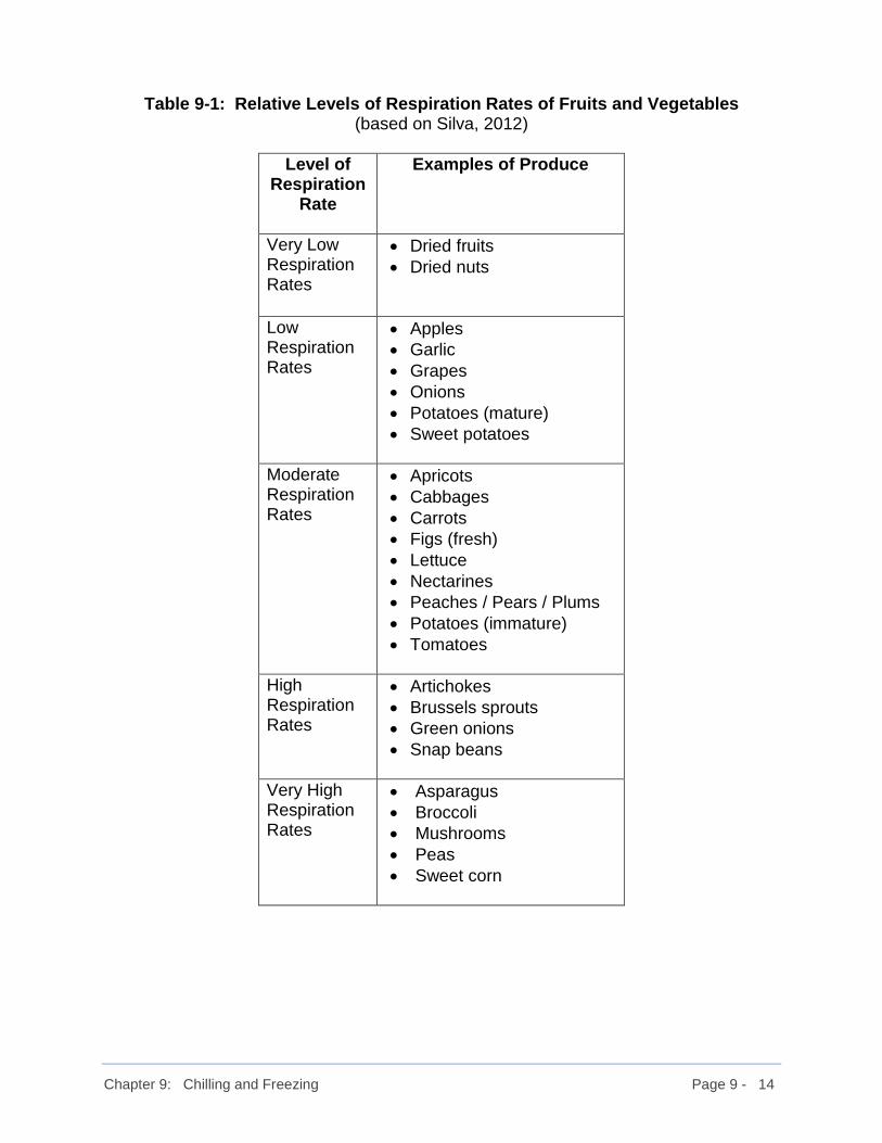
Chapter 9: Chilling and Freezing Page 9 - 14
Table 9-1: Relative Levels of Respiration Rates of Fruits and Vegetables (based on Silva, 2012)
Level of Respiration
Rate
Examples of Produce
Very Low Respiration Rates
• Dried fruits
• Dried nuts
Low Respiration Rates
• Apples
• Garlic
• Grapes
• Onions
• Potatoes (mature)
• Sweet potatoes
Moderate Respiration Rates
• Apricots
• Cabbages
• Carrots
• Figs (fresh)
• Lettuce
• Nectarines
• Peaches / Pears / Plums
• Potatoes (immature)
• Tomatoes
High Respiration Rates
• Artichokes
• Brussels sprouts
• Green onions
• Snap beans
Very High Respiration Rates
• Asparagus
• Broccoli
• Mushrooms
• Peas
• Sweet corn

Chapter 9: Chilling and Freezing Page 9 - 15
Even when stored at refrigerated temperatures of 2⁰C, the rate of
respiration has a major impact on how long these items will retain their freshness and quality. Table 9-2 shows the storage life of several fruits and vegetables under these conditions.
Table 9-2: Storage Life at 2⁰C
(Based on Gast)
Products Storage Life
Mushrooms (Very High Respiration Rates)
3 or 4 days
Lettuce (Moderate Respiration Rates)
2 weeks
Carrots (Moderate Respiration Rates)
7 to 9 months
Late Crop Potatoes (Low Respiration Rates)
Up to 10 months
There is an equation that is familiar to most people who have studied chemistry at the university level. That is the “Arrhenius Equation”. We won’t worry about taking an in-depth look at it. However, the important thing that we get from it is that the rate of a chemical reaction essentially doubles when the temperature is changed from 10°C to 20°C. If we consider that microbial growth is basically a chemical reaction, we would expect the rate at which the microorganisms grow to double if we changed the temperature from 10°C to 20°C. Looking at it from the opposite direction, let’s consider what would happen if we changed the temperature from 20°C,
which is close to room temperature, down to 10°C, which is a mild chilled temperature. It would be reasonable to expect the rate at which the microorganisms were growing to be halved. This means that a food material that lasted for two days at 20°C would last for four days at 10°C. If this trend holds true for a further temperature reduction to just above the freezing point of the material, we could expect an additional halving of the growth rate of the microorganisms. This would extend the storage life of four days at 10°C to about eight days at a temperature just above 0°C. While this might not be exactly the case, it does provide us with a sense of direction in how chilling can influence the growth rate of microorganisms. There are techniques whereby microbiologists can determine the actual effects of a ten degree change in temperature (on the Celsius scale) on the growth rate of specific microorganisms. They call this the “Q10 value”. It is not necessary to go into this degree of detail for our purposes here.

Chapter 9: Chilling and Freezing Page 9 - 16
9.10 Climacteric Ripening 9.10.1 What is Climacteric Ripening? While on the subject of ripening, we should discuss an additional aspect of this topic. Respiration rates are not always constant during storage, which is especially true for some fruits. There can be significant increases, or “spikes”, in the respiration rates as the fruits near their optimal ripeness. This is called “climacteric ripening”. Climacteric ripening is characterized by the production of ethylene which is a ripening hormone that accompanies the process. A knowledge of this behaviour can be used to control the ripening of climacteric fruits. Climacteric fruits include: apples, avocados, bananas, mangoes, peaches, pears, plums, and tomatoes. Figure 9-15 shows a diagrammatic representation of the ripening of a climacteric fruit. The vertical axis shows the rate of respiration and ethylene generation on a qualitative basis for a generic case. We do not need to specify actual values for our qualitative look at how climacteric ripening occurs. The horizontal axis of Figure 9-15 is really based on time, but it emphasizes the sequential stages of development of the fruit. Climacteric fruits are usually picked when they reach their full size but are still green, or not ripe. We can see this at the left side of the horizontal axis in
Figure 9-15. With time, the fruit begins to ripen as indicated by an increase in its respiration rate and the production of ethylene. The climacteric rise continues until the fruit reaches its fully ripened state. Following the climacteric peak, the rates of respiration and ethylene production begin to decrease as the fruit enters a period of senescence where the quality is diminishing and the fruit eventually rots. Ethylene production in some fruits is autocatalytic which means that production of a small amount of ethylene triggers the production of increasing amounts of ethylene to hasten ripening.
Figure 9-15: A qualitative look at respiration and ethylene production rates for climacteric fruits as they progress through the stages of ripening. Based on Saltveit (2016).

Chapter 9: Chilling and Freezing Page 9 - 17
9.10.2 Applications of Climacteric Ripening As stated above, a fundamental knowledge of climacteric ripening can be beneficial in helping to control the ripening of various fruits. By introducing ethylene into ripening chambers the process can be accelerated as required. It should be noted, however, that exposure times to ethylene must be limited to avoid complications. Bananas are an excellent example of a climacteric fruit. Bananas are picked when then are considered to be “commercially mature” and are shipped to their destinations where they are ripened by means of exposure to ethylene in ripening chambers. “Commercially mature” fruits like bananas, mangoes, and tomatoes are usually green and quite firm in order to resist damage during shipment and to prevent over-ripening before they reach the consumer. Fruits that are vine-ripened or tree-ripened have a much shorter shelf-life ahead of them and are usually sold at local markets where they will be purchased for more immediate use. Getting back to our example of bananas, the bananas will be harvested green and firm. Following shipment by air or ship to their port of destination, they will be placed in a controlled-environment ripening chamber. Ethylene gas is generated from ethanol and is introduced into the chamber at prescribed computer-controlled rates to maintain the desired concentration for the ripening of the bananas. It is
important to maintain the proper ethylene concentrations because improperly ripened bananas will lose their desired taste and texture. The bananas are not fully ripened in these chambers since they must still be distributed to supermarkets for sale to the consumer. At this stage, they may still be somewhat green, but will ripen in a short period of time in the consumer’s home. Figure 9-16 shows a pictorial representation of climacteric ripening where green bananas are exposed to ethylene gas (i.e., H2C=CH2).
Figure 9-16: Ripening of green bananas using ethylene gas.
In the home, an understanding of climacteric ripening can used to assist in the ripening of green bananas by placing them in a confined space with a high ethylene-producing fruit. Placing slices of apple (i.e., the ethylene gas source) in a paper bag with unripe bananas is one way to accomplish this. Figure 9-17 gives a pictorial representation of the reaction sequence.
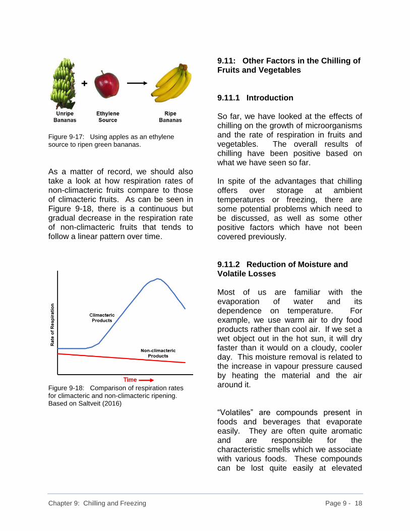
Chapter 9: Chilling and Freezing Page 9 - 18
Figure 9-17: Using apples as an ethylene source to ripen green bananas.
As a matter of record, we should also take a look at how respiration rates of non-climacteric fruits compare to those of climacteric fruits. As can be seen in Figure 9-18, there is a continuous but gradual decrease in the respiration rate of non-climacteric fruits that tends to follow a linear pattern over time.
Figure 9-18: Comparison of respiration rates for climacteric and non-climacteric ripening. Based on Saltveit (2016)
9.11: Other Factors in the Chilling of Fruits and Vegetables 9.11.1 Introduction So far, we have looked at the effects of chilling on the growth of microorganisms and the rate of respiration in fruits and vegetables. The overall results of chilling have been positive based on what we have seen so far. In spite of the advantages that chilling offers over storage at ambient temperatures or freezing, there are some potential problems which need to be discussed, as well as some other positive factors which have not been covered previously. 9.11.2 Reduction of Moisture and Volatile Losses Most of us are familiar with the evaporation of water and its dependence on temperature. For example, we use warm air to dry food products rather than cool air. If we set a wet object out in the hot sun, it will dry faster than it would on a cloudy, cooler day. This moisture removal is related to the increase in vapour pressure caused by heating the material and the air around it. “Volatiles” are compounds present in foods and beverages that evaporate easily. They are often quite aromatic and are responsible for the characteristic smells which we associate with various foods. These compounds can be lost quite easily at elevated
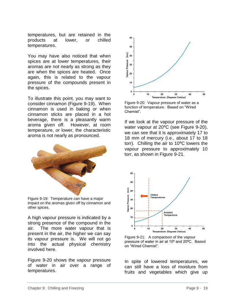
Chapter 9: Chilling and Freezing Page 9 - 19
temperatures, but are retained in the products at lower, or chilled temperatures. You may have also noticed that when spices are at lower temperatures, their aromas are not nearly as strong as they are when the spices are heated. Once again, this is related to the vapour pressure of the compounds present in the spices. To illustrate this point, you may want to consider cinnamon (Figure 9-19). When cinnamon is used in baking or when cinnamon sticks are placed in a hot beverage, there is a pleasantly warm aroma given off. However, at room temperature, or lower, the characteristic aroma is not nearly as pronounced.
Figure 9-19: Temperature can have a major impact on the aromas given off by cinnamon and other spices.
A high vapour pressure is indicated by a strong presence of the compound in the air. The more water vapour that is present in the air, the higher we can say its vapour pressure is. We will not go into the actual physical chemistry involved here. Figure 9-20 shows the vapour pressure of water in air over a range of temperatures.
Figure 9-20: Vapour pressure of water as a function of temperature. Based on “Wired Chemist”.
If we look at the vapour pressure of the water vapour at 20⁰C (see Figure 9-20),
we can see that it is approximately 17 to 18 mm of mercury (i.e., about 17 to 18 torr). Chilling the air to 10⁰C lowers the
vapour pressure to approximately 10 torr, as shown in Figure 9-21.
Figure 9-21: A comparison of the vapour pressure of water in air at 10⁰ and 20⁰C. Based on “Wired Chemist”.
In spite of lowered temperatures, we can still have a loss of moisture from fruits and vegetables which give up
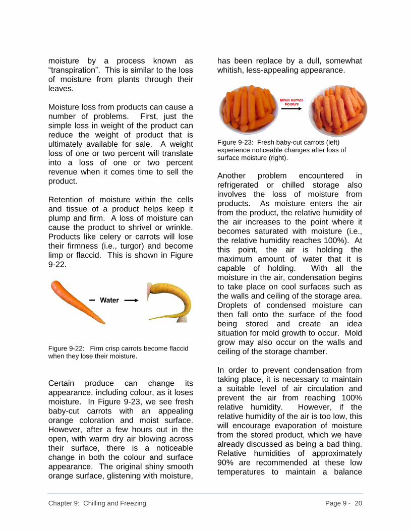
Chapter 9: Chilling and Freezing Page 9 - 20
moisture by a process known as “transpiration”. This is similar to the loss of moisture from plants through their leaves. Moisture loss from products can cause a number of problems. First, just the simple loss in weight of the product can reduce the weight of product that is ultimately available for sale. A weight loss of one or two percent will translate into a loss of one or two percent revenue when it comes time to sell the product. Retention of moisture within the cells and tissue of a product helps keep it plump and firm. A loss of moisture can cause the product to shrivel or wrinkle. Products like celery or carrots will lose their firmness (i.e., turgor) and become limp or flaccid. This is shown in Figure 9-22.
Figure 9-22: Firm crisp carrots become flaccid when they lose their moisture.
Certain produce can change its appearance, including colour, as it loses moisture. In Figure 9-23, we see fresh baby-cut carrots with an appealing orange coloration and moist surface. However, after a few hours out in the open, with warm dry air blowing across their surface, there is a noticeable change in both the colour and surface appearance. The original shiny smooth orange surface, glistening with moisture,
has been replace by a dull, somewhat whitish, less-appealing appearance.
Figure 9-23: Fresh baby-cut carrots (left) experience noticeable changes after loss of surface moisture (right).
Another problem encountered in refrigerated or chilled storage also involves the loss of moisture from products. As moisture enters the air from the product, the relative humidity of the air increases to the point where it becomes saturated with moisture (i.e., the relative humidity reaches 100%). At this point, the air is holding the maximum amount of water that it is capable of holding. With all the moisture in the air, condensation begins to take place on cool surfaces such as the walls and ceiling of the storage area. Droplets of condensed moisture can then fall onto the surface of the food being stored and create an idea situation for mold growth to occur. Mold grow may also occur on the walls and ceiling of the storage chamber. In order to prevent condensation from taking place, it is necessary to maintain a suitable level of air circulation and prevent the air from reaching 100% relative humidity. However, if the relative humidity of the air is too low, this will encourage evaporation of moisture from the stored product, which we have already discussed as being a bad thing. Relative humidities of approximately 90% are recommended at these low temperatures to maintain a balance

Chapter 9: Chilling and Freezing Page 9 - 21
between the loss of moisture and the occurrence of condensation. Warm temperatures and low relative humidities should be avoided (Figure 9-24).
Figure 9-24: Warm temperatures and moderate relative humidities may be comfortable for people, but are not good for storage of most produce.
9.11.3 Avoiding Moisture Loss In addition to controlling the relative humidity within the chilled storage chamber, there are additional steps which can be taken to reduce the loss of moisture from certain fruits and vegetables. Applying a thin coating of wax to the outer surface of the produce provides a barrier through which moisture cannot diffuse. Cucumbers and turnips, as well as peppers and tomatoes are routinely wax-coated to retain their freshness and prevent them from shrivelling due to moisture loss. An additional advantage of waxing is that it creates a smooth shiny surface, which is appreciated by consumers. Figure 9-25 shows a waxed sweet green pepper.
Figure 9-25: Waxed sweet green pepper.
Some produce, such as carrots, may be given a thin coating of a starch-based material to prevent the loss of moisture.
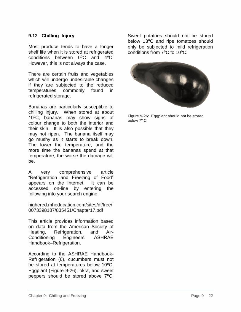
Chapter 9: Chilling and Freezing Page 9 - 22
9.12 Chilling Injury Most produce tends to have a longer shelf life when it is stored at refrigerated conditions between 0⁰C and 4⁰C.
However, this is not always the case. There are certain fruits and vegetables which will undergo undesirable changes if they are subjected to the reduced temperatures commonly found in refrigerated storage. Bananas are particularly susceptible to chilling injury. When stored at about 10⁰C, bananas may show signs of colour change to both the interior and their skin. It is also possible that they may not ripen. The banana itself may go mushy as it starts to break down. The lower the temperature, and the more time the bananas spend at that temperature, the worse the damage will be.
A very comprehensive article “Refrigeration and Freezing of Food” appears on the Internet. It can be accessed on-line by entering the following into your search engine:
highered.mheducation.com/sites/dl/free/0073398187/835451/Chapter17.pdf
This article provides information based on data from the American Society of Heating, Refrigeration, and Air-Conditioning Engineers’ ASHRAE Handbook–Refrigeration.
According to the ASHRAE Handbook-Refrigeration (6), cucumbers must not be stored at temperatures below 10⁰C.
Eggplant (Figure 9-26), okra, and sweet peppers should be stored above 7⁰C.
Sweet potatoes should not be stored below 13⁰C and ripe tomatoes should
only be subjected to mild refrigeration conditions from 7⁰C to 10⁰C.
Figure 9-26: Eggplant should not be stored below 7⁰ C

Chapter 9: Chilling and Freezing Page 9 - 23
9.13 Storing Potatoes Potatoes (Figure 9-27) and other starchy materials offer an additional challenge when it comes to storage. The “ASHRAE Handbook on Refrigeration” recommends storing main crop potatoes at temperatures between 3⁰C and 10⁰C. However, there is a
chance that within this temperature range, the starches present can be converted in their constituent sugars. This process is referred to as “cold sweetening” due to the increase in sugars. Problems arise when potatoes with these elevated sugar levels are used in frying applications such as making French fries or potato chips. Though a sequence referred to as the “Maillard Reaction”, a brown colouring can be produced through reactions between the reducing sugars and other compounds such as amino acids found within the flesh of the potatoes. Excessive browning and the potential development of off-flavours can lead to diminished quality and consumer dissatisfaction.
Figure 9-27: Potatoes may suffer from cold-sweetening if stored improperly.
9.14 Storing Bread Products Care must be taken considering the storage of bread and bread products (Figure 9-28). They should not be stored in a refrigerator, since this actually speeds up the process of staling by accelerating the process of “retrogradation”. Let’s take a look at what happens when bread is baked and why refrigeration is not recommended for bread.
Figure 9-28: Bread should not be stored in a refrigerator.
Wheat flour which is the basis for the bread is composed primarily of starch. As such, it has a crystalline structure composed of amylose and amylopectin molecules that are aligned in an organized fashion. When bread is made, the wheat flour is mixed with water and other ingredients and baked in an oven. As the temperature rises, the starches in the flour swell due to the uptake of water and they form a rather unstructured or formless network of starch molecules that could be considered to be a type of “gel”. The starch is now gelatinized. Once the baked bread is cooled, the gelatinized starches begin to re-align themselves into a structure similar to the one that existed before the dough was baked into bread. This process of re-

Chapter 9: Chilling and Freezing Page 9 - 24
organization or recrystallization of the starch molecules is referred to as “retrogradation”. At room temperature, retrogradation takes place rather slowly. However, if heat is removed from the bread and it is cooled to refrigerated temperatures, the crystalline structure of the starches becomes favoured over the non-crystalline alignments and staling is accelerated.
9.15 Freezing Fruits and Vegetables 9.15.1 Introduction Freezing fruits and vegetables is a logical extension of chilling them to temperatures just above their freezing point. In Chapter 5, we looked at freezing from the point of view of calculating how much heat must be removed from a given weight of material to change it from its thawed state to its frozen state (Figure 9-29). This involved a series of calculations as we lowered the temperature from its initial point to the freezing point of the material (Step ❶).
Then, we had to calculate the latent heat of fusion which is the amount of heat that has to be removed to freeze the water present in the material (Step ❷). Since this is a change of state,
there is no temperature change. Once the water is frozen, there is a third stage of the calculation to find the amount of heat that must be removed to lower the temperature from the freezing point to the final temperature (Step❸).
Figure 9-29: Steps involved in calculating amounts of heat removed in a freezing process.

Chapter 9: Chilling and Freezing Page 9 - 25
In this section, we will examine the behaviour of food materials as they are frozen and point out some of the problems encountered along the way. 9.15.2 Freezing Points of Liquid and Solid Foods Pure water freezes at 0°C (equivalent to 32°F). This is independent of the atmospheric pressure. However, as soon as a solute such as salt or sugar is dissolved in the water, it experiences a freezing point depression and the freezing point of the solution goes down. Since most fruits contain natural sugars, their freezing point will be lower than that of pure water. Oranges freeze at approximately -0.8°C, and apples freeze at about -1.1°C. Some varieties of grapes freeze at -2.1°C due to their high sugar content. Carrots freeze at -1.4°C, while leafy greens such as lettuce freeze at around -0.2°C or -0.3°C. Some cheeses don’t freeze until they reach -13.3°C. We will not worry about the calculation of the freezing point depression since it requires a rather involved chemistry-based derivation. You should be able to find the freezing point of most materials from web-based sources. The key thing is not to assume that fruits and vegetable freeze at the same temperature as pure water (i.e., 0°C).
9.15.3 Volume Change on Freezing Water is one of the few substances that expands when it freezes. You can easily see this when you look at ice cubes floating in a glass of water (Figure 9-30).
Figure 9-30: Coloured ice cubes floating in water.
This is an important thing to remember if you are freezing foods that have a high moisture content. In our home, we often freeze strawberry jam in tightly sealed glass jars to reduce the risk of spoilage. We only fill the jars about three-quarters full to allow room for the jam to expand. We have also frozen sauces and gravy in plastic containers for later use. Figure 9-31 illustrates what can happen if you freeze a glass jar full of water without leaving room for the liquid to expand. This makes the product totally unusable due to the presence of broken glass.
Figure 9-31: Glass jars full of water will crack when frozen due to expansion of the water.

Chapter 9: Chilling and Freezing Page 9 - 26
The true damage can be seen after the ice has melted (Figure 9-32).
Figure 9-32: Broken glass jar after ice has melted.
Shards of broken glass are a major safety hazard to consumers. As a general rule, use of glass is restricted to only packaging areas and is not allowed in processing areas per se.
9.16 Ice Crystal Formation During Freezing 9.16.1 Background Freezing products is not as simple as it may seem. It is not just putting the material in a freezer at a low temperature and letting it sit there until it freezes. Freezing begins at the microscopic level with the formation of tiny ice crystals. How these ice crystals form has a major impact on the quality of the frozen product. Ideally, we want very small ice crystals in our frozen fruits and vegetables. This reduces damage to the product that can result when large ice crystals form. 9.16.2 Freezing of Pure Water Let’s take a look at the freezing of pure water as an initial step in understanding the overall freezing process. For this experiment, a jar was filled with water to approximately three-quarters full to allow for the potential expansion of the water. A temperature probe was inserted through a small hole drilled in the metal lid. The tip of the probe was positioned at the centre of the water in the jar and the probe was secured in place with duct tape on the lid. The temperature was recorded every minute by taking time-lapsed photographs of the digital temperature display. Once the water was completely frozen, the test was halted.

Chapter 9: Chilling and Freezing Page 9 - 27
Results from the water freezing experiment were used to prepare a graph of temperature versus time, as shown in Figure 9-33.
Figure 9-33: Temperature versus time graph for freezing of water experiment. The surprising thing about the graph in Figure 9-33 is that the temperature of the water does not continue its downward path when it reaches the freezing point of 0°C. Instead, it holds a steady temperature at the freezing point for about six hours before it begins to go downwards once again. This behaviour was puzzling and certainly begged an explanation. What Figure 9-33 is showing us is that the water temperature falls at a fairly uniform rate from just under 24°C to 0°C in approximately 1.5 hours. There is no real mystery here. When the water reaches its freezing point of 0°C, the water molecules must undergo a change of state from a liquid to a solid. This is accomplished through the formation of ice crystals where the water molecules must go through a re-alignment process to form the ice crystal structures. To do so, the water
molecules must have a nucleation site upon which to form and grow. This process begins about 1.5 hours into the test. Before the temperature can drop below 0°C, enough heat must be removed from the system to cause all of the water molecules to form ice crystals around these nucleation sites. The longer this process takes, the bigger the ice crystals will grow. During the period from 1.5 hours to about 7.5 hours, the temperature is holding at 0°C. This is frequently referred to as the “critical zone”. Figure 9-34 is a close-up of a portion of Figure 9-33 and shows the critical zone as being the time during which the water is undergoing crystal growth.
Figure 9-34: A close-up view of Figure 9-33 showing the “Critical Zone” of ice crystal growth.
You can see from Figure 9-34 that the curve of temperature versus time remains in this “critical zone” for about 6 or 6.5 hours. Sometimes when you are freezing materials such as pure water or sugar solutions, you may see another rather perplexing situation. In one of the other tests for freezing water, the results shown in Figure 9-35 were obtained. The notable thing about this test run is the temperature of the water falling to -1.6°C and then rising suddenly to 0°C where it stayed for just
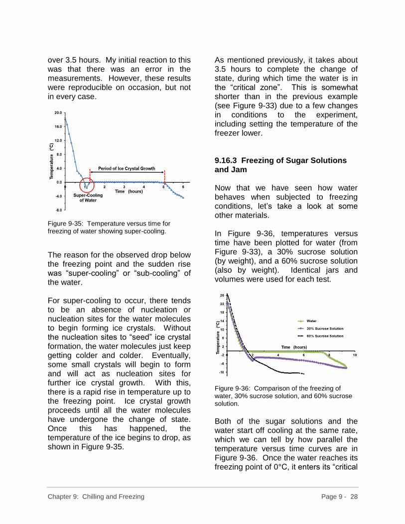
Chapter 9: Chilling and Freezing Page 9 - 28
over 3.5 hours. My initial reaction to this was that there was an error in the measurements. However, these results were reproducible on occasion, but not in every case.
Figure 9-35: Temperature versus time for freezing of water showing super-cooling.
The reason for the observed drop below the freezing point and the sudden rise was “super-cooling” or “sub-cooling” of the water. For super-cooling to occur, there tends to be an absence of nucleation or nucleation sites for the water molecules to begin forming ice crystals. Without the nucleation sites to “seed” ice crystal formation, the water molecules just keep getting colder and colder. Eventually, some small crystals will begin to form and will act as nucleation sites for further ice crystal growth. With this, there is a rapid rise in temperature up to the freezing point. Ice crystal growth proceeds until all the water molecules have undergone the change of state. Once this has happened, the temperature of the ice begins to drop, as shown in Figure 9-35.
As mentioned previously, it takes about 3.5 hours to complete the change of state, during which time the water is in the “critical zone”. This is somewhat shorter than in the previous example (see Figure 9-33) due to a few changes in conditions to the experiment, including setting the temperature of the freezer lower. 9.16.3 Freezing of Sugar Solutions and Jam Now that we have seen how water behaves when subjected to freezing conditions, let’s take a look at some other materials. In Figure 9-36, temperatures versus time have been plotted for water (from Figure 9-33), a 30% sucrose solution (by weight), and a 60% sucrose solution (also by weight). Identical jars and volumes were used for each test.
Figure 9-36: Comparison of the freezing of water, 30% sucrose solution, and 60% sucrose solution.
Both of the sugar solutions and the water start off cooling at the same rate, which we can tell by how parallel the temperature versus time curves are in Figure 9-36. Once the water reaches its freezing point of 0°C, it enters its “critical

Chapter 9: Chilling and Freezing Page 9 - 29
zone” where it stays until all water molecules have been changed to ice crystals. The 30% sucrose solution (purple curve) has a slightly lower freezing point than water and goes below 0°C. After being super-cooled, its temperature rises to its freezing point. There is a short horizontal portion to the line for the 30% sucrose solution before its temperature begins to drop and the frozen solution continues to become colder. This indicates that the “critical zone” for the 30% sucrose solution is shorter than for water. The sucrose in the solution may provide nucleation sites for the water after it has gone through its super-cooling. The 60% sucrose solution simply cools in a fairly uniform manner with no “critical zone”. There is a very slight disruption of the curve at about -4°C which may be where the water in the solution is actually going through its change of state. There is a levelling off of the temperature around -10°C and proceeds to cool slowly after that. This can be attributable to the temperature of the freezer in which the study was done. In Figure 9-37, the freezing of strawberry jam is compared to that of pure water.
Figure 9-37: Comparison of the freezing of strawberry jam and pure water.
The important thing to notice about the strawberry jam is that there is no “critical zone”. There is enough sugar and pectin in the jam to chemically bind the water which makes its behaviour much different than that of pure water. We should be careful not to read too much significance into the small oscillations in the curves at the lower temperatures. These may be attributable to the cycling of the freezer as its compressor turns on and off with the demand for chilling capacity in the freezer compartment. Overall, the strawberry jam freezes faster than the pure water which has spent six hours in its “critical zone”.

Chapter 9: Chilling and Freezing Page 9 - 30
9.16.4 Thawing of Water (Ice) and Strawberry Jam While we are on the topic of water and strawberry jam, it would seem logical to take a look at how these frozen materials behave when they are being thawed. The jars of frozen strawberry jam and water (i.e., ice) were placed on a mesh rack at room temperature to allow the ambient air to circulate around them. The temperatures were tracked at one-minute intervals until the temperatures began to approach that of the room air. Results of these tests are presented in Figure 9-38. Both materials started at approximately the same temperature. However, the water temperature rose faster than that of the strawberry jam until it approached its freezing / thawing point of 0°C. The more rapid rise in temperature could be attributed to the lower viscosity of the water which allowed heat to be transferred into the contents of the jar by both conduction and convection. Once it reached its freezing / thawing temperature, the water appeared to enter a “critical zone” similar to what it experienced during the freezing process. This lasted about five hours before the temperature began to climb once again. It was not until all water molecules had gone through their change of state from solid to liquid that the water could begin to heat up. In comparison, the temperature at the centre of the strawberry jam jar rose uniformly from its initial frozen temperature to about 8°C, where it
began to slow down. From this point onwards, its rate of temperature change slowed as it approached room temperature.
Figure 9-38: Comparison of thawing for frozen strawberry jam and ice.
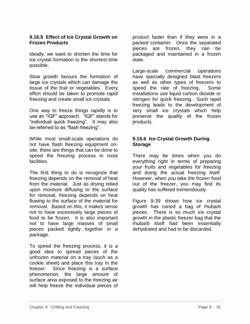
Chapter 9: Chilling and Freezing Page 9 - 31
9.16.5 Effect of Ice Crystal Growth on Frozen Products Ideally, we want to shorten the time for ice crystal formation to the shortest time possible. Slow growth favours the formation of large ice crystals which can damage the tissue of the fruit or vegetables. Every effort should be taken to promote rapid freezing and create small ice crystals. One way to freeze things rapidly is to use an “IQF” approach. “IQF” stands for “individual quick freezing”. It may also be referred to as “flash freezing”. While most small-scale operations do not have flash freezing equipment on-site, there are things that can be done to speed the freezing process in most facilities. The first thing to do is recognize that freezing depends on the removal of heat from the material. Just as drying relied upon moisture diffusing to the surface for removal, freezing depends on heat flowing to the surface of the material for removal. Based on this, it makes sense not to have excessively large pieces of food to be frozen. It is also important not to have large masses of small pieces packed tightly together in a package. To speed the freezing process, it is a good idea to spread pieces of the unfrozen material on a tray (such as a cookie sheet) and place this tray in the freezer. Since freezing is a surface phenomenon, the large amount of surface area exposed to the freezing air will help freeze the individual pieces of
product faster than if they were in a packed container. Once the separated pieces are frozen, they can be packaged and maintained in a frozen state. Large-scale commercial operations have specially designed blast freezers as well as other types of freezers to speed the rate of freezing. Some installations use liquid carbon dioxide or nitrogen for quick freezing. Such rapid freezing leads to the development of very small ice crystals which help preserve the quality of the frozen products. 9.16.6 Ice Crystal Growth During Storage There may be times when you do everything right in terms of preparing your fruits and vegetables for freezing and doing the actual freezing itself. However, when you take the frozen food out of the freezer, you may find its quality has suffered tremendously. Figure 9-39 shows how ice crystal growth has ruined a bag of rhubarb pieces. There is so much ice crystal growth in the plastic freezer bag that the rhubarb itself had been essentially dehydrated and had to be discarded.
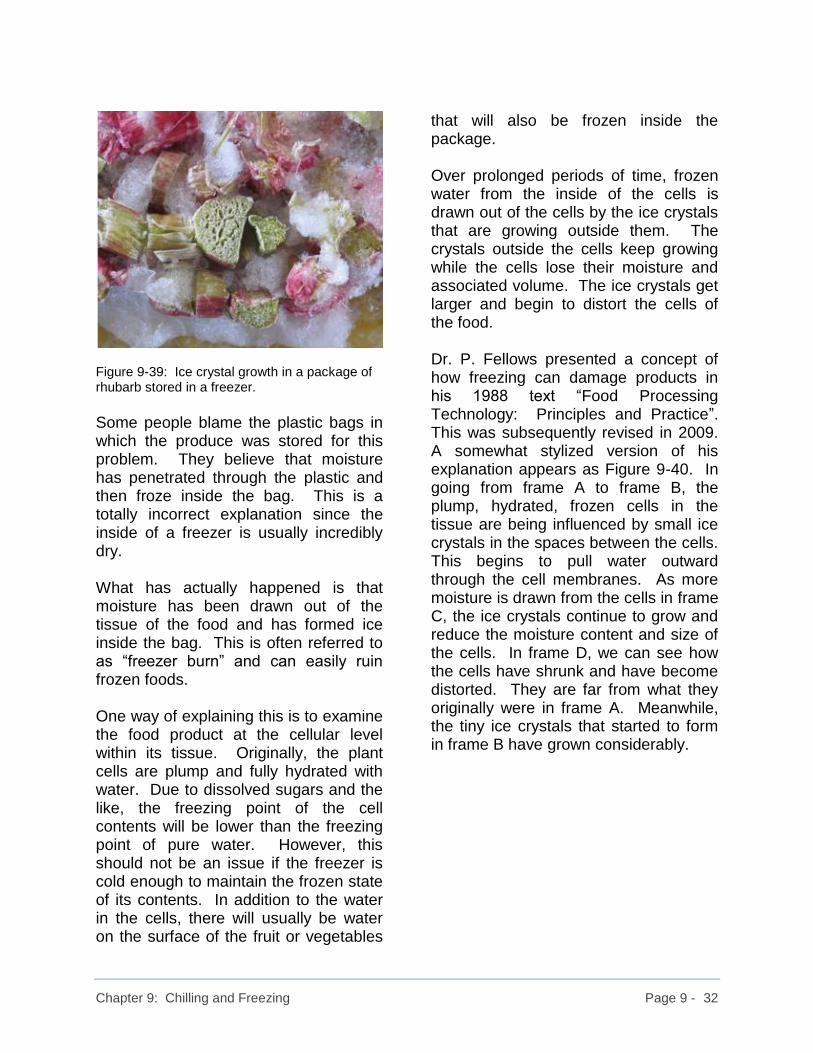
Chapter 9: Chilling and Freezing Page 9 - 32
Figure 9-39: Ice crystal growth in a package of rhubarb stored in a freezer.
Some people blame the plastic bags in which the produce was stored for this problem. They believe that moisture has penetrated through the plastic and then froze inside the bag. This is a totally incorrect explanation since the inside of a freezer is usually incredibly dry. What has actually happened is that moisture has been drawn out of the tissue of the food and has formed ice inside the bag. This is often referred to as “freezer burn” and can easily ruin frozen foods. One way of explaining this is to examine the food product at the cellular level within its tissue. Originally, the plant cells are plump and fully hydrated with water. Due to dissolved sugars and the like, the freezing point of the cell contents will be lower than the freezing point of pure water. However, this should not be an issue if the freezer is cold enough to maintain the frozen state of its contents. In addition to the water in the cells, there will usually be water on the surface of the fruit or vegetables
that will also be frozen inside the package. Over prolonged periods of time, frozen water from the inside of the cells is drawn out of the cells by the ice crystals that are growing outside them. The crystals outside the cells keep growing while the cells lose their moisture and associated volume. The ice crystals get larger and begin to distort the cells of the food. Dr. P. Fellows presented a concept of how freezing can damage products in his 1988 text “Food Processing Technology: Principles and Practice”. This was subsequently revised in 2009. A somewhat stylized version of his explanation appears as Figure 9-40. In going from frame A to frame B, the plump, hydrated, frozen cells in the tissue are being influenced by small ice crystals in the spaces between the cells. This begins to pull water outward through the cell membranes. As more moisture is drawn from the cells in frame C, the ice crystals continue to grow and reduce the moisture content and size of the cells. In frame D, we can see how the cells have shrunk and have become distorted. They are far from what they originally were in frame A. Meanwhile, the tiny ice crystals that started to form in frame B have grown considerably.
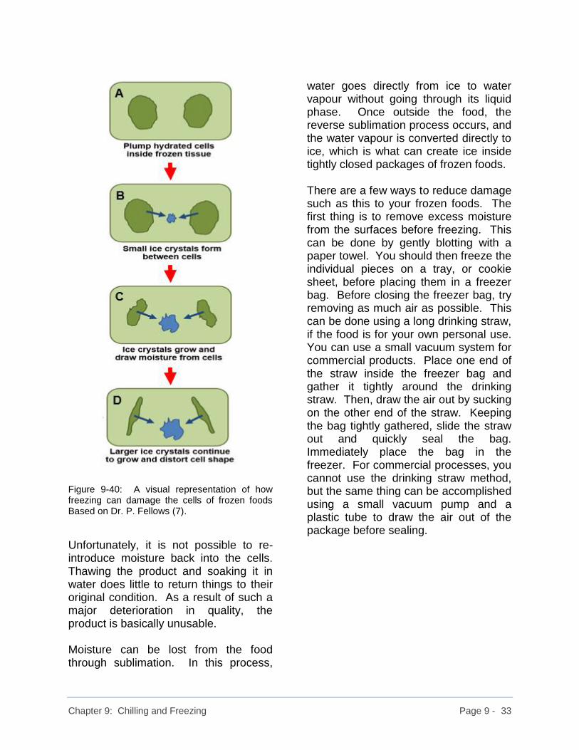
Chapter 9: Chilling and Freezing Page 9 - 33
Figure 9-40: A visual representation of how freezing can damage the cells of frozen foods Based on Dr. P. Fellows (7).
Unfortunately, it is not possible to re-introduce moisture back into the cells. Thawing the product and soaking it in water does little to return things to their original condition. As a result of such a major deterioration in quality, the product is basically unusable. Moisture can be lost from the food through sublimation. In this process,
water goes directly from ice to water vapour without going through its liquid phase. Once outside the food, the reverse sublimation process occurs, and the water vapour is converted directly to ice, which is what can create ice inside tightly closed packages of frozen foods. There are a few ways to reduce damage such as this to your frozen foods. The first thing is to remove excess moisture from the surfaces before freezing. This can be done by gently blotting with a paper towel. You should then freeze the individual pieces on a tray, or cookie sheet, before placing them in a freezer bag. Before closing the freezer bag, try removing as much air as possible. This can be done using a long drinking straw, if the food is for your own personal use. You can use a small vacuum system for commercial products. Place one end of the straw inside the freezer bag and gather it tightly around the drinking straw. Then, draw the air out by sucking on the other end of the straw. Keeping the bag tightly gathered, slide the straw out and quickly seal the bag. Immediately place the bag in the freezer. For commercial processes, you cannot use the drinking straw method, but the same thing can be accomplished using a small vacuum pump and a plastic tube to draw the air out of the package before sealing.

Chapter 9: Chilling and Freezing Page 9 - 34
9.17 Calculation of Freezing Times Anyone interested in the mathematical methods of calculating the time required to freeze a material in an industrial process is urged to consider Plank’s Equation. Plank developed his model in 1913. It was modified in 1949 by Ede, and has been a useful tool in estimating freezing times since then. Its one major deficiency is that it assumes the material is already at its freezing temperature. Plank’s Equation then calculates the time required for the actual change of state in freezing to take place. While this gives a somewhat low estimate of the freezing time, it is still a popular equation. In 1986, Pham proposed a more complicated model to predict freezing times. However, due to its inherent complexity, Pham’s model has not replaced that of Plank. These models require a knowledge of heat transfer through solid materials and rate of heat transfer from surfaces. Calculations of this type are not typically done in small-scale food processing operations. Therefore, I have not included them here. Should you be considering the purchase of a blast freezer or other similar device for flash freezing your product, it is recommended that you work with a reliable and reputable equipment supplier to address the issues associated with the design of such equipment,
9.18 Summary Comments Chilling and freezing are important technologies that food processors have available to prolong storage life and enhance product quality. There are many aspects that cannot be covered here due primarily to the restriction of space. There are also some highly complicated treatments such as the calculation of freezing times which we have only touched on here. It is not my intention to delve deeply into such challenging mathematical treatments when for most of us, the truly important thing is understanding the basic principles. Should you wish to find additional information on this topic, there are numerous sources available on-line and in high quality textbooks written by expert researchers in this particular area.

Chapter 9: Chilling and Freezing Page 9 - 35
9.19 References ASHRAE. “The 1986 ASHRAE Handbook – Refrigeration”. American Society of Heating, Refrigerating, and Air Conditioning Engineers. Fellows, P.J. “Food Processing Technology: Principles and Practice” (Third Edition). CRC Press, Woodhead Publishing Limited, Cambridge, 2009. Gast, Karen L.B. “Storage Conditions: Fruits and Vegetables”. Bulleting #4135. University of Maine, Cooperative Extension Publications. Available on-line at: https://extension.umaine.edu/publications/4135e/ (accessed March 2018). Hazeleger, Wilma C., Jeroen A. Wouters, Frank M. Rombouts, and Tjakko Abee. “Physiological Activity of Campylobacter jejuni Far below the Minimal Growth Temperature Appl Environ Microbiol. 1998 Oct; 64(10): 3917–3922. Available on-line at: www.ncbi.nlm.nih.gov/pmc/articles/PMC106578/ Accessed April 2018. highered.mheducation.com/sites/dl/free/0073398187/835451/Chapter17.pdf Accessed March 2018. Rahman, M. Shafiur, Editor. “Handbook of Food Preservation” Second Edition. CRC Press, Taylor and Frances Group, Boca Raton, Florida, USA, 2007.
Saltveit, M.E. “The Commercial Storage of Fruits, Vegetables, and Florist and Nursery Stocks”. United States Department of Agriculture, Agricultural Research Service, Agriculture Handbook, revised 2016. Available on-line at: www.ars.usda.gov/ARSUserFiles/oc/np/CommercialStorage/CommercialStorage.pdf (accessed March 2018). Silva, Erin. “Respiration and Ethylene and Their Relationship to Postharvest Handling”. Organic Agriculture, March 5, 2012. University of Wisconsin. Available on-line at: articles.extension.org/pages/18354/respiration_and_ethylene_and_their_relationship_to_postharvest_handling (accessed March 2018). Wired Chemist. “Vapor Pressure of Water from 0°C to 100°C”. Table of data available on-line at: www.wiredchemist.com/chemistry/data/vapor-pressure (accessed March 2018).

Chapter 10: Separation and Concentration Page 10 - 1
10. Separation and Concentration 10.1 Introduction Food processors routinely use a wide variety of methods to concentrate solutions and to separate components in mixtures. Commonly used methods rely on differences in physical properties of compounds present in the mixtures. These may include such things as particle size (Figure 10-1) density (Figure 10-2), solubility, boiling point, freezing point, or molecular weight. Other separation processes may involve chemical properties including chemical bonding.
Figure 10-1: A sieve (or strainer) is an example of separating mixtures of solids and liquids on the basis of particle size.
Most people are familiar with sand particles settling to the bottom of a pail of water. When the sand and water mixture is stirred, the sand particles can be held in suspension by the motion of the water. However, once the motion of the water slows sufficiently, the particles fall rapidly to the bottom (Figure 10-2). Here the difference in density between the sand (1,600 kg per cubic metre) and
the water (1,000 kg per cubic metre) is great enough to permit the sand to settle under the force of gravity (Perry and Green, 1997).
Figure 10-2: Sand suspended in moving water (left side) will settle when the motion of the water slows (right side).
Often processors are attempting to remove excess water from solutions which have a low concentration of a particular solute. The reasons for this are diverse and numerous. They can range from recovery of valuable ingredients to waste treatment. Separations range from removing large particulates such as foreign objects in shipments of grain to removal of undesired chemical species at the molecular level. 10.2 Membrane Filtration A popular and economical type of separation process is based on particle size differences. Coarse screens are used to separate sand from gravel, and paper filters are used in coffee makers to hold the coffee grounds while hot water is poured through them. Similar separations can be accomplished by using filtration at the molecular level. Small molecules (i.e., those of relatively low molecular weight) can be separated from larger molecules (i.e., those of

Chapter 10: Separation and Concentration Page 10 - 2
relatively high molecular weight) through the use of porous membrane materials. Membranes can be made of a variety of polymeric materials (e.g., cellulose acetate, polysulphones, etc.) designed to suit specific applications. These applications include foods as well as beverages, pharmaceuticals, dairy, waste treatment, water purification, chemical processing, and many more. For convenience, membrane filtration processes can be classified according to the size range of particles that they remove from solution. Sizes are generally expressed in microns, where one micron is a millionth of a metre, or a thousandth of a millimetre. General classifications are shown in Table 10-1. Table 10-1: Classification of Membrane Filtration Techniques by Particle Size
Technique Particle Size Range
in microns (μm)
Particle Filtration over 1 μm
Microfiltration 0.05 to 5 μm
Ultrafiltration 0.005 to 0.2 μm
Nanofiltration 0.0008 to 0.01 μm
Hyperfiltration 0.0001 to 0.003 μm
These sizes are based on various sources and the ranges tend to overlap. The important thing is to recognize the incredibly small sizes which are being concentrated. In examining the particle sizes listed above, it is quite apparent that there is a certain degree of overlap between a particular size range for a membrane filtration category and the one above and below it. It should also be noted that hyperfiltration is more frequently referred to as “reverse osmosis”.
The basic principle of membrane filtration is shown schematically in Figures 10-3a and 10-3b. A solution of large molecules (shown as larger dark circles) and smaller molecules is contained on one side of a porous membrane (Figure 10-3a). The pores of the membrane itself are sized to permit the solvent and smaller molecules to pass through while excluding the larger molecules. It is only required that a pressure be exerted on the solution of small and large molecules to force the solvent and smaller molecules through the membrane.
Figure 10-3a: A solution of small and large molecules prior to filtration through a membrane.
When pressure is applied as in Figure 10-3b, the solvent and smaller molecules pass through the membrane and leave the larger ones behind. This creates a concentrated solution of larger molecules on one side of the membrane (which also contains the same concentration of smaller molecules as

Chapter 10: Separation and Concentration Page 10 - 3
was present in the original solution). The solution passing through the membrane is free of the large molecules and maintains the same concentration of smaller molecules as was present in the original solution. Therefore, the process has successfully concentrated the larger molecules, or conversely, it has successfully removed the larger molecules from solution.
Figure 10-3b: Applying pressure forces only solvent and small molecules through the membrane filter.
In order to maximize the amount of membrane surface area within a given volume, hollow fibre membranes are often used. The membranes are formed into very fine long tubes. The ends of these tubes are “potted” in an epoxy resin so that their open ends are exposed. By placing the potted hollow fibres inside a cartridge, a solution to be filtered can be pumped into these tubes. Water and small molecules can pass through the membrane material, but larger molecules cannot fit through the membrane pores. As a result, the
solution coming out the other end of the cartridge will be more concentrated in the high molecular weight compounds than the feed going into the cartridge. Figure 10-4 shows a hollow fibre membrane filtration cartridge. The terms “permeate” and “retentate” are defined in the next section.
Figure 10-4: A hollow fibre membrane filtration cartridge.
Figure 10-5 shows an end view of the cartridge with the end cap removed. You can see the openings from each of the hollow fibres and how fine they are.

Chapter 10: Separation and Concentration Page 10 - 4
Figure 10-5: An end view of the membrane cartridge showing the openings of the potted hollow fibres.
Figure 10-6 is a photo of the membrane cartridge cut away to expose the fine hollow fibres. Each hollow fibre has the diameter of a coarse hair.
Figure 10-6: Cut-away of the membrane cartridge showing the individual hollow fibres.
10.2.1 Terminology Before proceeding too much further, some basic terminology must be established. Figure 10-7 will aid in this. Feed is the solution that enters the system containing a mixture of larger and smaller molecules in a solvent (usually water).
Permeate is the liquid and the molecules it contains that pass through the membrane. Retentate is the liquid (and molecules it contains) that does not pass through the membrane, but is retained on the feed side of the membrane. Flux rate is the term used to describe the rate at which permeate goes through the membrane. It is expressed in units of volume per area of membrane per unit time (e.g.: litres per square metre of membrane per day; or, U.S. gallons per square foot per day, etc.). Tangential flow is a flow pattern used in membrane processes where the feed is passed across the membrane surface rather than straight down upon it. In this way, the flow continuously sweeps across the membrane surface and carries away much of the material that might otherwise foul or plug the membrane and its pores.
Figure 10-7: Diagram illustrating terms associated with membrane filtration.
In performing mass balances on membrane separation systems, the following relationship is useful:

Chapter 10: Separation and Concentration Page 10 - 5
Weight of Feed Solution = Weight of + Weight of Retentate Permeate Solution Solution
(Eq’n 10-1)
In many cases, the density differences between the feed solution and the permeate and retentate streams are so small that the approximate relationship can be written:
Volume of Feed Solution ≈
Volume of + Volume of Retentate Permeate Solution Solution (Eq’n 10-2) While this is only an approximation, it is often reliable enough for rough calculations. Do not base exacting calculations on volumes. Use the weight (i.e., mass) of the solutions as the basis of your calculations. 10.2.2 Methods of Operation Membrane units can be used in both batch and continuous systems. In some cases, the processor may have only one membrane processing unit. A batch filtration process would be carried out to obtain the desired results. Here, the retentate would be recirculated back to the feed tank while the permeate was collected in a separate tank. The solution in the feed tank would become more and more concentrated and lower in volume as the procedure progressed. Once the desired
degree of concentration is achieved, the procedure is stopped (Figure 10-8). As an example, a processor may have 500 litres of a 1% starch solution. By recirculating the retentate back to the feed tank in an ultrafiltration process, the process can be run until a desired final concentration of perhaps 4% starch is reached in the feed tank. At the end of the run, there would be approximately 125 litres of 4% starch solution in the feed tank and approximately 375 litres of permeate would have been collected.
Figure 10-8: A batch membrane filtration process showing return of retentate to the feed tank.
When using a series of membrane filtration units in a continuous system, the retentate from one unit can be used as the feed for the next unit. By the end of the process, the retentate has become more concentrated than the feed solution, and the permeate streams from the individual units can be combined into a single stream. The system would have to be configured so as to obtain the required separation in each step to arrive at the desired final retentate concentration (Figure 10-9).
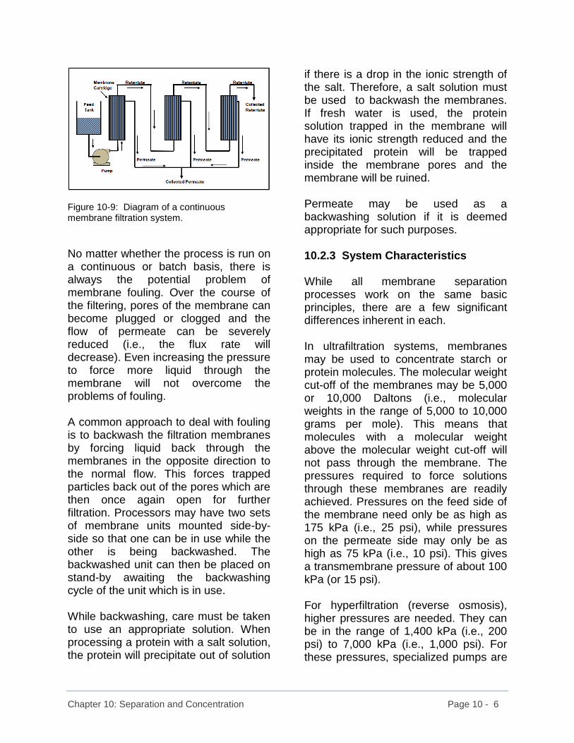
Chapter 10: Separation and Concentration Page 10 - 6
Figure 10-9: Diagram of a continuous membrane filtration system.
No matter whether the process is run on a continuous or batch basis, there is always the potential problem of membrane fouling. Over the course of the filtering, pores of the membrane can become plugged or clogged and the flow of permeate can be severely reduced (i.e., the flux rate will decrease). Even increasing the pressure to force more liquid through the membrane will not overcome the problems of fouling. A common approach to deal with fouling is to backwash the filtration membranes by forcing liquid back through the membranes in the opposite direction to the normal flow. This forces trapped particles back out of the pores which are then once again open for further filtration. Processors may have two sets of membrane units mounted side-by-side so that one can be in use while the other is being backwashed. The backwashed unit can then be placed on stand-by awaiting the backwashing cycle of the unit which is in use. While backwashing, care must be taken to use an appropriate solution. When processing a protein with a salt solution, the protein will precipitate out of solution
if there is a drop in the ionic strength of the salt. Therefore, a salt solution must be used to backwash the membranes. If fresh water is used, the protein solution trapped in the membrane will have its ionic strength reduced and the precipitated protein will be trapped inside the membrane pores and the membrane will be ruined. Permeate may be used as a backwashing solution if it is deemed appropriate for such purposes. 10.2.3 System Characteristics While all membrane separation processes work on the same basic principles, there are a few significant differences inherent in each. In ultrafiltration systems, membranes may be used to concentrate starch or protein molecules. The molecular weight cut-off of the membranes may be 5,000 or 10,000 Daltons (i.e., molecular weights in the range of 5,000 to 10,000 grams per mole). This means that molecules with a molecular weight above the molecular weight cut-off will not pass through the membrane. The pressures required to force solutions through these membranes are readily achieved. Pressures on the feed side of the membrane need only be as high as 175 kPa (i.e., 25 psi), while pressures on the permeate side may only be as high as 75 kPa (i.e., 10 psi). This gives a transmembrane pressure of about 100 kPa (or 15 psi). For hyperfiltration (reverse osmosis), higher pressures are needed. They can be in the range of 1,400 kPa (i.e., 200 psi) to 7,000 kPa (i.e., 1,000 psi). For these pressures, specialized pumps are

Chapter 10: Separation and Concentration Page 10 - 7
required. Prior to the development of new membrane materials, pressures three or four times higher than these current values were needed. Hyperfiltration membranes filter out very small molecular species and are used to desalinate sea water for drinking. The actual mechanism of removing sodium and chloride ions is not based solely on size exclusion, but ionic charge plays a major role as well. 10.2.4 Reverse Osmosis As its name implies, reverse osmosis is based on the reversal of a process known as “osmosis”. Osmosis is the principle whereby a solvent (usually water) in an area of low solute concentration travels across a semi-permeable membrane layer to an area of higher solute concentration on the other side of the membrane. Osmosis is how plants take in water through their roots from the soil. Here, the inner portion of the plant’s roots contains sugars in solution (e.g., sap-like material). The soil in which the root is located contains water and dissolved minerals, but the concentration of these is much less than the concentration of the solution inside the plant root. There is a natural tendency of the liquid to flow across the root membrane from the area of lower concentration to the area of higher concentration in an attempt to equalize the concentration. This is the process of “osmosis” which is shown conceptually in Figure 10-10. The driving force for this process is called the “osmotic pressure” and can
be seen as a height differential in Figure 10-10 when the system is at equilibrium.
Figure 10-10: Diagram to show concept of osmosis with initial conditions (top) and equilibrium conditions (bottom).
To carry out the reverse of the osmosis process, it is necessary to overcome the osmotic pressure of the system by applying an external pressure. In Figure 10-11, a pressure is being exerted that not only overcomes the natural osmotic pressure across the semi-permeable membrane, but that actually forces liquid to travel in the opposite direction. In the reverse osmosis process for an aqueous solution, the retentate concentration increases while the permeate is generally pure water. It should be noted that there are now reverse osmosis units operating at low enough pressures to make them suitable for in-home water purification use.

Chapter 10: Separation and Concentration Page 10 - 8
Figure 10-11: Diagram to show concept of reverse osmosis with initial conditions (top) and after pressure has been applied to the sugar solution (bottom).
10.2.5 Comparison of Membrane Filtration Techniques Figures 10-12a through 10-12d show the relationships between the various membranes and the particles which can pass through them.
Figure 10-12a: Microfiltration membranes allow all but particulates and colloids to pass through.
Figure 10-12b: Ultrafiltration membranes exclude high molecular weight compounds.

Chapter 10: Separation and Concentration Page 10 - 9
Figure 10-12c: Nanofiltration membranes allow low molecular weight compounds to pass through.
Figure 10-12d: Hyperfiltration membranes (or reverse osmosis membranes) allow only water molecules to pass through
10.2.6 Concentration and Volume Reduction Factors In a membrane separation process, the ratio between the initial feed and the final retentate is used to express the “concentration factor”, or “volume reduction factor”. Concentration Factor = Weight of Feed Solution Weight of Retentate
(Eq’n 10-3) Volume Reduction Factor = Volume of Feed Solution Volume of Retentate
(Eq’n 10-4) Concentration factors may also be also be calculated on the basis of the concentration of a solute (i.e., the material dissolved in the solvent). However, you need to be careful to select the solute that is actually being concentrated. For example, in some protein solutions, salt may also be present to help solubilize the protein. In an ultrafiltration process, the protein will be concentrated, but the salt will pass through the pores in the membrane. Therefore, you cannot base the concentration factor on the salt, since its concentration in the permeate and in the feed will be the same. You must calculate the concentration factor on the basis of the protein which is being concentrated. The concentrations for this calculation need to be on a weight basis. For example 5.0% by weight would be used.

Chapter 10: Separation and Concentration Page 10 - 10
Concentration Factor = Concentration in the Retentate Concentration in the Feed
(Eq’n 10-5) The volume reduction factor is frequently used in industrial processes to report the degree of concentration of a solution due to the fact that liquid volumes are often easier to measure than weights. As an example, if 1,200 litres of feed solution are concentrated to 400 litres of retentate, the volume reduction factor for the process would be 3.0.
10.2.7 Sample Calculation 10-1 A process to recover protein from soy meal or pea meal uses a 3.0% salt solution (i.e., 3.0% by weight) to solubilize the protein from the vegetable meal. Once the protein is dissolved, the solution is concentrated by means of ultrafiltration in preparation for further processing steps. Consider a protein recovery test run where an 800 litre batch of solution is being processed. The initial concentration of protein in the salt solution is 1.5% by weight and its specific gravity is 1.025. After being filtered through a 5,000 Dalton molecular weight cut-off membrane, the weight of the retentate collected is 223.6 kg. The protein concentration in the retentate is 5.5%. Unfortunately, the process operator threw out the permeate before it could be weighed and analyzed for its salt and protein content. Additional information: Salt (sodium chloride or NaCl) has a molecular weight of 58.5 Daltons and generally dissociates into smaller ions. The protein being recovered in this process has a molecular weight of over 10,000 Daltons. A Dalton is a unit of molecular mass with units of grams per mole. a. How much permeate was collected? b. How much salt and protein are in the
permeate? Is this process functioning well? Why, or why not?
c. What is the concentration of salt in
the retentate? Is this surprising?

Chapter 10: Separation and Concentration Page 10 - 11
d. What is the concentration factor for this process ?
e. What additional piece or pieces of
information would be needed to calculate the volume of the permeate?
Solution: The first step is to prepare a diagram of the process. Figure 10-13 shows the process with all given data and identifies missing information.
Figure 10-13: Diagram for sample calculation 10-1.
Part a: First, the weight of the initial solution must be calculated. Weight of initial solution = volume x density = 800 litres | 1.025 kg | litre = 820 kg
Weight of permeate = weight of initial solution - weight of (i.e., feed solution) retentate = 820 kg - 223.6 kg = 596.4 kg Therefore, the weight of the permeate is 596.4 kg Part b: To find the weights of protein and salt in the permeate, the weights of protein and salt in the feed and retentate solutions must be found. Weight of protein in feed solution = 820 kg x 0.015 = 12.30 kg Weight of salt in feed = 820 kg x 0.03 = 24.6 kg Weight of protein in retentate = 223.6 kg x 0.055 = 12.30 kg Weight of salt in retentate = 223.6 kg x 0.03 = 6.71 kg Protein in permeate = protein in feed - protein in retentate = 12.30 kg - 12.30 kg = 0.0 kg Salt in permeate = salt in feed - salt in retentate = 24.6 kg - 6.71 kg = 17.89 kg Therefore, there is no protein and 17.89 kg of salt in the permeate.

Chapter 10: Separation and Concentration Page 10 - 12
Since there is no protein passing through the membrane in the permeate, the process would appear to be running well. Part c: % salt in permeate = weight of salt in permeate X 100% weight of permeate = 17.89 kg x 100% 596.4 kg = 3.0% Therefore, the concentration of salt in the permeate is 3.0%, which is not surprising since the salt is small enough to pass through the ultrafiltration membrane along with the water. The salt is not concentrated in the process. Part d: Concentration factor = weight of feed solution weight of retentate = 820 kg 223.6 kg = 3.67 (dimensionless) Therefore, the concentration factor for the process is 3.67. We can also look at the concentration factor on the basis of the percentage by weight of the solutes in solution. Let’s start by looking at the concentration factor for just the protein.
It has a concentration of 1.5% protein in the feed and 5.5% protein in the retentate. Substituting these values into the appropriate equation gives: Concentration factor = Concentration of protein in retentate Concentration of protein in feed = 5.5% by weight 1.5% by weight = 3.67 (dimensionless) This is the same result as we obtained from the other equation. Now, let’s base the calculation on just the salt that is present. The concentration of salt is 3.0% by weight in the feed and 3.0% by weight in the retentate. Concentration factor = Concentration of salt in retentate Concentration of salt in feed = 3.0% by weight 3.0% by weight = 1.00 (dimensionless) This indicates that no concentration is taking place for the salt, which is correct since the salt is small enough to pass through the pores of the ultrafiltration membrane. Similarly, if we take the total solute concentration in the feed and retentate streams, we will get a misleading answer. We have 1.5% protein and

Chapter 10: Separation and Concentration Page 10 - 13
3.0% salt in the feed for a total of 4.5% by weight. In the retentate, we have 5.5% protein and 3.0% salt, for a total of 8.5% by weight. Concentration factor = Concentration of solutes in retentate Concentration of solutes in feed = 8.5% by weight 4.5% by weight = 1.89 (dimensionless) Before accepting the calculated value of the concentration factor as being correct, you need to examine what is being concentrated. Two of these three calculations give us erroneous values since they involve salt which is not being concentrated. Part e: The density (or specific gravity) of the permeate solution would be necessary in order to calculate its volume.
10.2.8 Applications of Membrane Separation Processes Table 10-2 lists a variety of applications of membrane technology processes in the food and beverage related industries. There are numerous other related areas where membrane technologies are employed. These include:
• Biotechnology • Pharmaceuticals • Waste water treatment • Textiles and dyes
Many “sizing” chemicals used to coat paper, and adhesives have a plant origin (e.g., starches), and a number of dyes can be extracted from plant materials. Mention of textiles and dyes also serves as a reminder of the broad range of applications of membrane technology.
Chapter 10: Separation and Concentration Page 10 - 14
Table 10-2 Examples of Applications of
Membrane Separation Processes (compiled from various sources)
Food and Beverages:
• General clarification and concentration processes (e.g., juices, beer, wine, syrups, and edible oils)
• Gelatin concentration • Flavour extract processing • Waste water recovery • Protein extraction processes • Vinegar clarification
Dairy:
• Whey protein concentrates • Cheese brine clarification • Demineralization of whey • Concentration of whey, skim milk,
and whole milk • Fractionation of milk for cheese
making • Defatting of whey
10.3 Freeze Concentration When a liquid food product is subjected to freezing, not all of the components present freeze at exactly the same time or temperature. Some of the water will freeze first and will form ice crystals in the product. The remaining unfrozen product will be more concentrated, since the solute species were not included in the ice crystals that formed. By slowly freezing a liquid product, a processor can form a slush of ice crystals in a concentrated liquid product. The ice crystals can be removed with a mesh screen, or by centrifugation, leaving the concentrated solution behind. In practice, there will be some solute species trapped in the ice crystals, but this is generally a minor loss of less than 1%. Such a process has been applied to orange juice concentration with considerable success. The benefits of freeze concentration include the lack of a heat treatment step which can vaporize volatile flavor components and aromatics. Figure 10-14 shows a schematic diagram for a typical freeze concentration process.

Chapter 10: Separation and Concentration Page 10 - 15
Figure 10-14: Schematic diagram of a freeze concentration process
10.3.1 Sample Calculation 10-2 In a freeze concentration process, an 800 kg batch of a blend of wild-berry juices (12.0% solids) is considered too delicate to concentrate by heat treatment. The processors use freeze concentration to concentrate the juice to 45% solids. 202.0 kg of concentrated wild-berry product are collected. If there is less than 1.0% by weight of solids present in the ice that is removed, the process would be considered to have an acceptable level of loss. Would the process described here be functioning satisfactorily, or would it need some maintenance work?
Solution: Figure 10-15 provides a starting point for solving this problem.
Figure 10-15: Diagram for Sample Calculation 10-2.
The weight of the ice and the amount of solids it contains must be determined in order to calculate the percentage of solids present in the ice.

Chapter 10: Separation and Concentration Page 10 - 16
Weight of ice = weight of feed - weight of solution concentrate = 800 kg - 202 kg = 598 kg (this includes water and solids) The weight of solids in the ice will be the difference between the weight of solids in the feed solution and the weight of solids in the concentrate. Weight of solids in feed solution = 800 kg x 0.12 = 96.0 kg Weight of solids in concentrate = 202 kg x 0.45 = 90.9 kg Solids lost in ice = solids in feed - solids in solution concentrate = 96.0 kg - 90.9 kg = 5.1 kg % solids in ice = weight of solids x 100% weight of ice = 5.1 kg X 100% 598 kg = 0.85% Therefore, the amount of solids in the ice is 0.85%. Since this is below the 1.0% weight limit for the process, the process would appear to be running in an acceptable manner.
10.4 Centrifugation Separation of components by centrifugation is based on a difference in density between the components to be separated. In the first section of this chapter, we mentioned how sand will settle out of suspension in water when the motion of the water slows. Another example of separation by density is oil and water. Since the oil is less dense than water and will not dissolve in the water, it forms a layer on top of the water (Figure 10-16).
Figure 10-16: Oil layer on water.
In many cases, the density differences between the components to be separated are not large enough to facilitate separation by gravity. Certain salad dressings will separate after standing for considerable periods of time. The tiny oil droplets in the emulsion (i.e., the salad dressing) will float to the top and the product must be shaken vigorously to get the oil back into the mixture before using it. Here, separation of the components is not desirable.
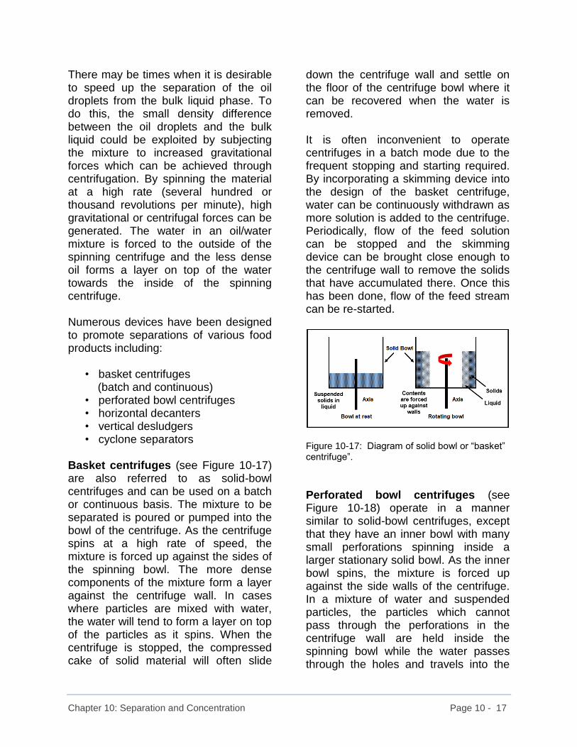
Chapter 10: Separation and Concentration Page 10 - 17
There may be times when it is desirable to speed up the separation of the oil droplets from the bulk liquid phase. To do this, the small density difference between the oil droplets and the bulk liquid could be exploited by subjecting the mixture to increased gravitational forces which can be achieved through centrifugation. By spinning the material at a high rate (several hundred or thousand revolutions per minute), high gravitational or centrifugal forces can be generated. The water in an oil/water mixture is forced to the outside of the spinning centrifuge and the less dense oil forms a layer on top of the water towards the inside of the spinning centrifuge. Numerous devices have been designed to promote separations of various food products including:
• basket centrifuges (batch and continuous)
• perforated bowl centrifuges • horizontal decanters • vertical desludgers • cyclone separators
Basket centrifuges (see Figure 10-17) are also referred to as solid-bowl centrifuges and can be used on a batch or continuous basis. The mixture to be separated is poured or pumped into the bowl of the centrifuge. As the centrifuge spins at a high rate of speed, the mixture is forced up against the sides of the spinning bowl. The more dense components of the mixture form a layer against the centrifuge wall. In cases where particles are mixed with water, the water will tend to form a layer on top of the particles as it spins. When the centrifuge is stopped, the compressed cake of solid material will often slide
down the centrifuge wall and settle on the floor of the centrifuge bowl where it can be recovered when the water is removed. It is often inconvenient to operate centrifuges in a batch mode due to the frequent stopping and starting required. By incorporating a skimming device into the design of the basket centrifuge, water can be continuously withdrawn as more solution is added to the centrifuge. Periodically, flow of the feed solution can be stopped and the skimming device can be brought close enough to the centrifuge wall to remove the solids that have accumulated there. Once this has been done, flow of the feed stream can be re-started.
Figure 10-17: Diagram of solid bowl or “basket” centrifuge”.
Perforated bowl centrifuges (see Figure 10-18) operate in a manner similar to solid-bowl centrifuges, except that they have an inner bowl with many small perforations spinning inside a larger stationary solid bowl. As the inner bowl spins, the mixture is forced up against the side walls of the centrifuge. In a mixture of water and suspended particles, the particles which cannot pass through the perforations in the centrifuge wall are held inside the spinning bowl while the water passes through the holes and travels into the
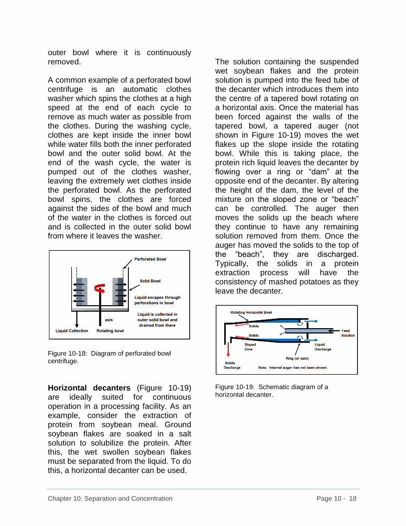
Chapter 10: Separation and Concentration Page 10 - 18
outer bowl where it is continuously removed. A common example of a perforated bowl centrifuge is an automatic clothes washer which spins the clothes at a high speed at the end of each cycle to remove as much water as possible from the clothes. During the washing cycle, clothes are kept inside the inner bowl while water fills both the inner perforated bowl and the outer solid bowl. At the end of the wash cycle, the water is pumped out of the clothes washer, leaving the extremely wet clothes inside the perforated bowl. As the perforated bowl spins, the clothes are forced against the sides of the bowl and much of the water in the clothes is forced out and is collected in the outer solid bowl from where it leaves the washer.
Figure 10-18: Diagram of perforated bowl centrifuge.
Horizontal decanters (Figure 10-19) are ideally suited for continuous operation in a processing facility. As an example, consider the extraction of protein from soybean meal. Ground soybean flakes are soaked in a salt solution to solubilize the protein. After this, the wet swollen soybean flakes must be separated from the liquid. To do this, a horizontal decanter can be used.
The solution containing the suspended wet soybean flakes and the protein solution is pumped into the feed tube of the decanter which introduces them into the centre of a tapered bowl rotating on a horizontal axis. Once the material has been forced against the walls of the tapered bowl, a tapered auger (not shown in Figure 10-19) moves the wet flakes up the slope inside the rotating bowl. While this is taking place, the protein rich liquid leaves the decanter by flowing over a ring or “dam” at the opposite end of the decanter. By altering the height of the dam, the level of the mixture on the sloped zone or “beach” can be controlled. The auger then moves the solids up the beach where they continue to have any remaining solution removed from them. Once the auger has moved the solids to the top of the “beach”, they are discharged. Typically, the solids in a protein extraction process will have the consistency of mashed potatoes as they leave the decanter.
Figure 10-19: Schematic diagram of a horizontal decanter.
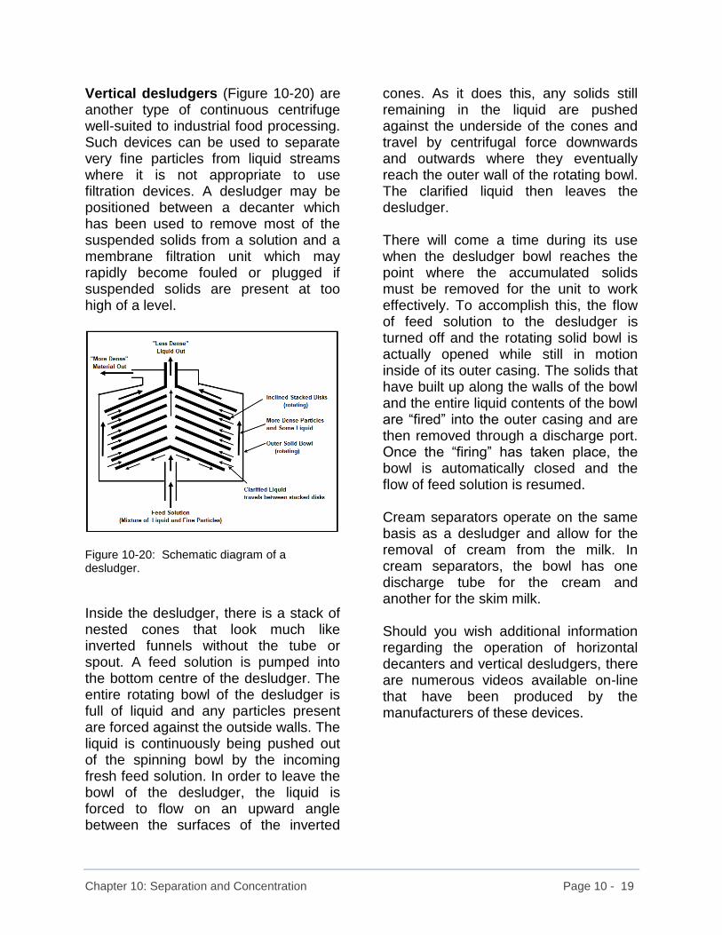
Chapter 10: Separation and Concentration Page 10 - 19
Vertical desludgers (Figure 10-20) are another type of continuous centrifuge well-suited to industrial food processing. Such devices can be used to separate very fine particles from liquid streams where it is not appropriate to use filtration devices. A desludger may be positioned between a decanter which has been used to remove most of the suspended solids from a solution and a membrane filtration unit which may rapidly become fouled or plugged if suspended solids are present at too high of a level.
Figure 10-20: Schematic diagram of a desludger.
Inside the desludger, there is a stack of nested cones that look much like inverted funnels without the tube or spout. A feed solution is pumped into the bottom centre of the desludger. The entire rotating bowl of the desludger is full of liquid and any particles present are forced against the outside walls. The liquid is continuously being pushed out of the spinning bowl by the incoming fresh feed solution. In order to leave the bowl of the desludger, the liquid is forced to flow on an upward angle between the surfaces of the inverted
cones. As it does this, any solids still remaining in the liquid are pushed against the underside of the cones and travel by centrifugal force downwards and outwards where they eventually reach the outer wall of the rotating bowl. The clarified liquid then leaves the desludger. There will come a time during its use when the desludger bowl reaches the point where the accumulated solids must be removed for the unit to work effectively. To accomplish this, the flow of feed solution to the desludger is turned off and the rotating solid bowl is actually opened while still in motion inside of its outer casing. The solids that have built up along the walls of the bowl and the entire liquid contents of the bowl are “fired” into the outer casing and are then removed through a discharge port. Once the “firing” has taken place, the bowl is automatically closed and the flow of feed solution is resumed. Cream separators operate on the same basis as a desludger and allow for the removal of cream from the milk. In cream separators, the bowl has one discharge tube for the cream and another for the skim milk. Should you wish additional information regarding the operation of horizontal decanters and vertical desludgers, there are numerous videos available on-line that have been produced by the manufacturers of these devices.
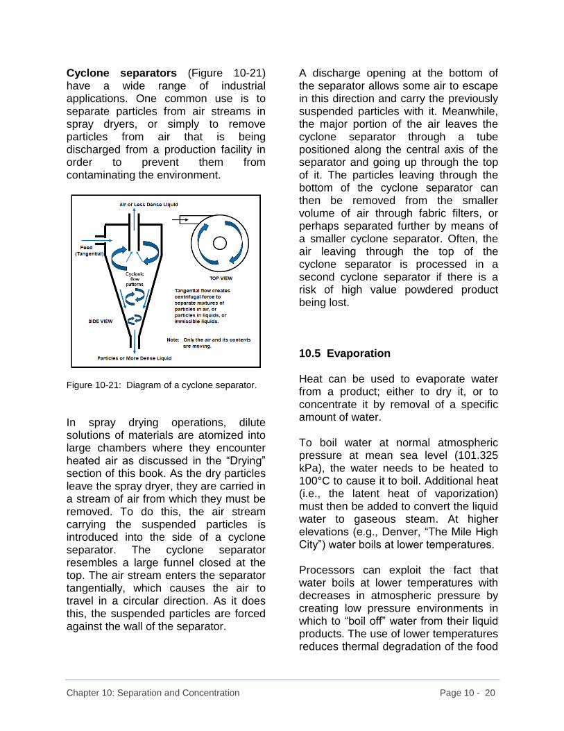
Chapter 10: Separation and Concentration Page 10 - 20
Cyclone separators (Figure 10-21) have a wide range of industrial applications. One common use is to separate particles from air streams in spray dryers, or simply to remove particles from air that is being discharged from a production facility in order to prevent them from contaminating the environment.
Figure 10-21: Diagram of a cyclone separator.
In spray drying operations, dilute solutions of materials are atomized into large chambers where they encounter heated air as discussed in the “Drying” section of this book. As the dry particles leave the spray dryer, they are carried in a stream of air from which they must be removed. To do this, the air stream carrying the suspended particles is introduced into the side of a cyclone separator. The cyclone separator resembles a large funnel closed at the top. The air stream enters the separator tangentially, which causes the air to travel in a circular direction. As it does this, the suspended particles are forced against the wall of the separator.
A discharge opening at the bottom of the separator allows some air to escape in this direction and carry the previously suspended particles with it. Meanwhile, the major portion of the air leaves the cyclone separator through a tube positioned along the central axis of the separator and going up through the top of it. The particles leaving through the bottom of the cyclone separator can then be removed from the smaller volume of air through fabric filters, or perhaps separated further by means of a smaller cyclone separator. Often, the air leaving through the top of the cyclone separator is processed in a second cyclone separator if there is a risk of high value powdered product being lost. 10.5 Evaporation Heat can be used to evaporate water from a product; either to dry it, or to concentrate it by removal of a specific amount of water. To boil water at normal atmospheric pressure at mean sea level (101.325 kPa), the water needs to be heated to 100°C to cause it to boil. Additional heat (i.e., the latent heat of vaporization) must then be added to convert the liquid water to gaseous steam. At higher elevations (e.g., Denver, “The Mile High City”) water boils at lower temperatures. Processors can exploit the fact that water boils at lower temperatures with decreases in atmospheric pressure by creating low pressure environments in which to “boil off” water from their liquid products. The use of lower temperatures reduces thermal degradation of the food

Chapter 10: Separation and Concentration Page 10 - 21
product and is more economical from an energy utilization perspective than evaporation at higher temperatures. Evaporation in a closed vessel under vacuum also allows flavour components that would otherwise be lost, to be recovered and added back to the product at a later stage in the process. These closed vessels with applied vacuum are collectively referred to as “evaporators”. There are numerous designs for evaporators, each aimed at a specific use. They can be used singly (Figure 10-22), or in series. In engineering terms, each evaporator may be referred to as an “effect”. As many as seven evaporators (i.e., a seven “effect” evaporator system) can be arranged so that each successive evaporator concentrates the discharge from the previous evaporator until the final desired concentration is reached. Through use of more modern and sophisticated processes such as mechanical vapor recompression, large amounts of water can be evaporated from solutions economically and efficiently.
Figure 10-22: Diagram showing operation of a typical single-effect evaporator.
10.6 Ion Exchange 10.6.1 Basic Principles Ion exchange is widely used in water softening applications. Hard water is characterized by its inability to form suds when cleaning solutions such as soap are used. This is due to the presence of calcium and magnesium ions which are divalent (i.e., have a double positive charge) and form complexes with the soap that prevent the formation of suds. They can actually create a soap curd or film on surfaces. In addition, the hardness ions may also complex with ingredients in liquid food products and lead to a reduction in quality attributes such as taste. It is generally desirable to remove these ions from the water stream before using it for a product ingredient or even as the basis for a cleaning solution. This can be done through ion exchange. Ion exchange resins are prepared from polymeric materials which are formed into beads. Each bead has numerous sites onto which sodium (or hydrogen) ions can freely bond under suitable conditions of concentration. However, the resin has a greater affinity for divalent ions such as calcium and magnesium ions (or even trivalent ions such as aluminium: Al3+) which are what normally give water its “hardness”. When “hard” water containing calcium and magnesium ions is passed through a column or bed of ion exchange resin, the resin exchanges its sodium ions for the more preferred calcium and magnesium ions. These hardness ions are thereby taken out of solution and are replaced by sodium ions. For each calcium ion (Ca2+) or magnesium ion
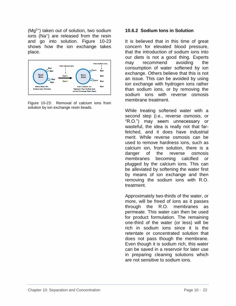
Chapter 10: Separation and Concentration Page 10 - 22
(Mg2+) taken out of solution, two sodium ions (Na+) are released from the resin and go into solution. Figure 10-23 shows how the ion exchange takes place.
Figure 10-23: Removal of calcium ions from solution by ion exchange resin beads.
10.6.2 Sodium Ions in Solution It is believed that in this time of great concern for elevated blood pressure, that the introduction of sodium ions into our diets is not a good thing. Experts may recommend avoiding the consumption of water softened by ion exchange. Others believe that this is not an issue. This can be avoided by using ion exchange with hydrogen ions rather than sodium ions, or by removing the sodium ions with reverse osmosis membrane treatment. While treating softened water with a second step (i.e., reverse osmosis, or “R.O.”) may seem unnecessary or wasteful, the idea is really not that far-fetched, and it does have industrial merit. While reverse osmosis can be used to remove hardness ions, such as calcium ion, from solution, there is a danger of the reverse osmosis membranes becoming calcified or plugged by the calcium ions. This can be alleviated by softening the water first by means of ion exchange and then removing the sodium ions with R.O. treatment. Approximately two-thirds of the water, or more, will be freed of ions as it passes through the R.O. membranes as permeate. This water can then be used for product formulation. The remaining one-third of the water (or less) will be rich in sodium ions since it is the retentate or concentrated solution that does not pass though the membrane. Even though it is sodium rich, this water can be saved in a reservoir for later use in preparing cleaning solutions which are not sensitive to sodium ions.

Chapter 10: Separation and Concentration Page 10 - 23
10.6.3 Regeneration of Ion Exchange Resins There will come a time when the capacity of the ion exchange resin to exchange sodium ions for calcium and magnesium ions is exhausted. This occurs when all available sodium has been transferred from its sites on the resin, and these sites are in turn taken up by the hardness ions. At this point, the ion exchange resin must be “regenerated”. To regenerate an ion exchange resin, the process water flow to the ion exchange column is shut down. A concentrated salt solution made from sodium chloride crystals in a salt tank reservoir is then pumped into the ion exchange column and allowed to remain there for a prescribed time period. During this time, the extremely high sodium ion concentration forces the resin to release the calcium and magnesium ions and once again bind sodium to the active sites. Having allowed sufficient time for the regeneration to take place, the resin column is then flushed with fresh water to remove the salt solution containing the calcium and magnesium ions from the column which is sent to a drain for disposal. All of the regeneration procedures are automatically controlled by valves, flowmeters, and timers. In Figure 10-24, there are two ion exchange columns operating in parallel. While one is being used to soften the water, the other is being regenerated. Note the positions of the various valves. Open and shaded circles have been used in Figure 10-24 to show the state of the valves rather
than using the conventional valve symbols.
Figure 10-24: Diagram of an ion exchange system with regeneration of the column.
A major concern regarding the use of ion exchange for water softening is the amount of salt that it releases into the environment through the concentrated brine solution discharged following each regeneration sequence.

Chapter 10: Separation and Concentration Page 10 - 24
10.6.4 Food-Related Applications of Ion Exchange The major application of ion exchange in the food industry would appear to be the removal of hardness ions from water streams. Since water is the primary ingredient in beverage formulations, it is obvious that the higher the quality of the water used in batching, the higher the quality of the finished product will be. Water should also be softened prior to being used in boilers for steam generation. Failure to remove calcium can result in scale build-up similar to the “lime” that can be seen building up on the inside of kettles used to boil hard water in the home. There are various processes where ion exchange resins are used to recover high-value components that are present in dilute concentrations in processing solutions. Ion exchange can also be used to remove impurities in refining processes such as that for sugar.
10.7 Adsorption Activated charcoal or activated carbon can be used to remove organic material from solution. Columns of activated carbon are frequently placed in series with ion exchange columns as part of the overall water treatment process. Organic compounds that may cause “off-odours” in solution can be removed through their adsorption onto the active sites of the activated carbon. Care must be taken to replace the activated carbon filters at regular intervals - even during periods when they are not in use. Organic material clinging to the activated carbon may become the substrate for the growth of microorganisms that can grow in these columns when the columns are not in use. Once the columns are started up again, the microorganisms can enter the process water stream. During periods of continuous use, this is not an issue. If there are no significant “down times” between uses, it is only necessary to be concerned about the actual capacity of the activated carbon so that it may be replaced at the appropriate time before its capacity for the removal of organic material is exceeded. You may be familiar with home water treatment systems that use a small replaceable cartridge in a pitcher-like container. The main component inside this cartridge is activated carbon. As water travels through the activated carbon, organic matter that can cause off-flavours or odours is removed. Figure 10-25 shows the activated carbon removed from a used water filtration cartridge.

Chapter 10: Separation and Concentration Page 10 - 25
Figure 10-25: Activated carbon from the cartridge of a home water treatment system.
10.8 Chromatographic Techniques 10.8.1 Basic Principles Chromatographic separation is a major topic in its own right, and it is not the intention of this section to cover it in great detail. There are numerous methods of chromatographic separations that can be discussed. Some separate materials on the basis of charge, while others rely on size for their separations. In some respects, chromatographic techniques may resemble ion exchange. Even though chromatography columns may be packed with resins as in the case of ion exchange columns, there may be no ion exchange actually taking place. Mixtures containing solutes can be passed through these columns and one of the solutes may be selectively adsorbed onto the gel in the column. Consider a mixture of glucose and fructose in solution passing through a resin bed with calcium ions fixed to it. Fructose has a high attraction to the calcium ion and may be adsorbed or its passage through the column may be slowed compared to that of the glucose molecules by the column resin. The glucose may pass through with very little of it being adsorbed. Once the separation has taken place, conditions in the column can be altered slightly to promote the desorption of the fructose and the column can then be readied for additional separations.

Chapter 10: Separation and Concentration Page 10 - 26
10.9 Solvent Extraction Solvent extraction processes can range from incredibly simple to very complex. As its name implies, the basic principle is to use a solvent of some type (e.g., water or alcohol) to solubilize and thereby extract a compound found in a solid substance. In industrial food processes, it is value-added compounds that are generally extracted. Let’s begin this section by examining one of the most simple and common solvent extractions. Many of us have prepared a cup of tea by placing a tea bag or tea leaves in boiling water. After a short time, you can see the solvent extraction taking place as the mixture begins to change colour. Not only are coloured compounds extracted, such as polyphenols in black tea, but caffeine is also drawn out of the tea leaves. Figure 10-26 shows solvent extraction using hot water from black tea.
Figure 10-26: Solvent extraction from a teabag using boiling water as the solvent.
Commercial solvent extractions may involve extracting beneficial molecular species from plant material. Among these is the extraction of proteins and oils, which we will now examine briefly.
Oils of vegetable origin, such as Canola or soybean oils, are very important in today’s food industry. They offer a healthy alternative to animal-based fats and oils. It is the extraction of these oils from the vegetable materials which is of major importance in food applications. Fats and oils are not readily soluble in water. Generally what happens when oils are mixed with water is that they separate into two distinct layers with the less dense oil floating on the more dense water. If oil and water mixture is homogenized, the result is a dispersion of tiny oil droplets in the continuous water phase, or tiny droplets of water in the continuous oil phase. In either case, an emulsion is formed that may or may not be stable over a period of time. The question that arises from the information above is, if oil is not soluble in water, how can the oil be removed from the Canola or soybeans in the first place? One answer to this is “solvent extraction”. Vegetable oils are soluble in organic solvents such as hexane. The Canola or soybeans can be crushed to form a meal. Up to 40% by weight of this meal may be oil. Hexane can then be run over the meal to extract or solubilize the oil. Next, the hexane-oil mixture can be processed in vacuum evaporators to remove the hexane and recover it for further use in the extraction system. This process is highly efficient, recovering almost all of the oil present in the crushed meal. It is also a relatively safe process, but there are concerns over the effects of the use of hexane on human health and the environment. Another example of solvent extraction is the production of tofu in which proteins are extracted from soybeans using hot

Chapter 10: Separation and Concentration Page 10 - 27
water. The protein can then be recovered from this “soy milk” by forming a protein curd and removing it from the mixture by filtration (Figure 10-27)
Figure 10-27: Protein curd formed in soy milk (left photo) will settle (right photo) and can be recovered by filtration.
In the past, caffeine was removed from coffee beans through solvent extraction with methylene chloride. Methylene chloride is a main ingredient in compounds used to strip paint and varnish from wood furniture (this is no longer practised). Later, salt water was used to decaffeinate coffee and tea. One story states that a chest of tea fell into the ocean and was later recovered. When the leaves were washed to remove the salt water and later used to make the beverage, there was a substantially lower level of caffeine than for tea leaves not exposed to salt water. Caffeine removal has kept up with recent technological developments and is now using the most up-to-date techniques, as shall be shown below. A key aspect of solvent extraction is the development of a process that uses a
“safe” extraction liquid that is also “environmentally friendly”. 10.10 Supercritical Fluid Extraction Supercritical fluid extraction is an attractive alternative to using organic solvents such as hexane, or acetone, or methylene chloride. Instead of using these harsh organic solvents, it employs a gas such as carbon dioxide under “critical” conditions of temperature and pressure to solubilize the material to be removed or recovered. When subjected to high pressures (e.g., over 7 million Pascals, or > 7 megaPascals) and a critical temperature of approximately 31°C, carbon dioxide (CO2) behaves as a supercritical fluid. It has a density near that of its liquid state, but still behaves as if it were a gas that can penetrate into various materials. In a supercritical fluid extraction (SCFE) process, the material to be processed is placed in a column capable of withstanding the high pressures required. The supercritical CO2 is then introduced. As it is pumped through the columns, the supercritical fluid solubilizes various compounds and removes them from the bulk of the material in the column. Once the supercritical fluid leaves the column, it is separated from the solute that it is carrying by lowering the pressure in a special chamber. An example of supercritical extraction would be the removal of caffeine from coffee beans or tea leaves. Not only are the decaffeinated beans or tea leaves a desirable end product, but the caffeine

Chapter 10: Separation and Concentration Page 10 - 28
may also have important uses in the pharmaceutical industry. (Figure 10-28).
Figure 10-28: Schematic diagram of a supercritical solvent extraction process.
Other applications include the removal of delicate flavour oils from plant materials. Mint oil can be extracted from mint leaves and retain its refreshing aroma and taste (Figure 10-29). Usage of this technology is expanding. However, it is a relatively expensive method and is limited to value-added materials that can support the cost at the present time.
Figure 10-29: Mint oil (in cup) can be extracted from fresh mint leaves using supercritical solvent extraction.
The advantages of supercritical fluid extraction are quite apparent when one considers that carbon dioxide is not as harmful as other organic solvents. To separate carbon dioxide from the extracted material, it is only necessary to reduce the pressure and the CO2 will flash off as a gas leaving no harmful residue. The recovered carbon dioxide can be re-pressurized and sent back to the process for subsequent extractions.

Chapter 10: Separation and Concentration Page 10 - 29
10.11 Precipitation 10.11.1 Basic Principles Precipitation is the process of having dissolved materials settle out of solution. There are several methods of inducing precipitation of materials from solution. One way is to add solutes to the solution which will complex with ions present or molecular species to form insoluble salts that precipitate out (i.e., fall to the bottom of the vessel in which the solution is contained). An example of this would be a solution containing calcium ions and oxalate groups. When a solution of calcium chloride is added to a solution of ammonium oxalate, an insoluble calcium oxalate will precipitate out of solution (Figure 10-30).
Figure 10-30: Formation of calcium oxalate by the reaction of ammonium oxalate and calcium chloride.
Here is the chemical reaction that is taking place (Figure 10-31).
Figure 10-31: Reaction between calcium chloride and ammonium oxalate.
In water, the calcium chloride salt (CaCl2) separates, or dissociates, into one calcium ion (Ca++) and two chloride ions (Cl-). The ammonium oxalate ((NH4)2C2O4) dissociates into two ammonium groups (NH4
+) and one oxalate group (C2O4
=). The calcium ion and oxalate group then bond together to form calcium oxalate (CaC2O4) which is an insoluble solid that settles to the bottom of the liquid as a precipitate. Each chloride ion can form an ionic compound with one of the ammonium groups to give ammonium chloride (NH4Cl), which remains in solution. This reaction is shown in Figure 10-32. The subscript “aq” in brackets means that the material is dissolved in an aqueous solution. The subscript “s” means that the material is a solid, and the downward pointing arrow beside it indicates that it settles out of solution as a precipitate.
Figure 10-32: Chemical equation for the reaction between calcium chloride and ammonium oxalate.

Chapter 10: Separation and Concentration Page 10 - 30
The above example is not one that would be used in a food product application, but it does have relevance in human health. Oxalate can occur naturally in such things as rhubarb leaves. These oxalates can react with calcium in the body to create calcium oxalate and form insoluble kidney stones. 10.11.2 Protein Recovery by Precipitation The extraction of protein from vegetable material such as soybean meal is an interesting process. To solubilize the protein, salt is added to the water being used to soak the soybean meal. While the protein is in solution, the extracted soybean meal can be sent through various centrifugation steps such as decanting and / or desludging. The protein can then be concentrated by ultrafiltration through membranes with pores small enough to let the salt water solution pass through, yet retain the proteins in the retentate solution. The protein will still be present in a salt solution since the sodium chloride is not concentrated or removed during ultrafiltration. If the concentrated protein solution is then dilute with fresh cold water, the concentration of the sodium chloride will be reduced, as will the protein concentration. The important thing here is that once the concentration of sodium chloride solution falls below the ionic strength required to solubilize the protein, the protein precipitates out of solution. The excess liquid can be syphoned away from the precipitate. The precipitated protein can then be
recovered by centrifugation to remove even more of the water, and then it can be freeze-dried for future use. A schematic diagram of this process appears as Figure 10-33.
Figure 10-33: Process for solubilizing and precipitating protein.
10.12 Summary Comments In this chapter, we have attempted to show how solutions can be concentrated, or how particles can be removed from suspensions can by various physical methods. These can be quite useful techniques for small-scale processing operations. As we learn more about the beneficial properties of various plants and the components contained within them, extraction methods will become more important to us. Solvent extraction is a rather straight-forward method of isolating these value-added components.

Chapter 10: Separation and Concentration Page 10 - 31
10.13 References The majority of information in this chapter is based on first-hand experience while in industry and from lecture notes put together for food processing courses. As such, there are no formal references. That being said, there are many useful sources of information available on-line to augment the material presented here.

Chapter 11: Closing Comments and Lists of Figures and Tables Page 11 - 1
11. Closing Comments
In the preceding chapters, we have examined a variety of technologies frequently employed in food processing. Realistically, it is impossible to cover every single area of food processing. As a result, I am sure certain things have been omitted that some readers may consider critical to a work of this nature. In putting this guide together, I have tried to capture the essentials of what would be needed for small-scale food processors and entrepreneurs. The core disciplines selected are based on my own personal experiences in the food industry, working in government, and instructing food processing courses in academia. Most of all, working closely with various groups in a number of countries as we conducted food processing workshops, has clearly demonstrated the need for information in a number of these specific topics. Drying and thermal processing are particularly important. Once you have gained familiarity with the fundamentals, you can then delve more deeply into specific areas of interest and explore the technologies more deeply. One thing that is not covered in any great depth here is “Cleaning and Sanitation” plus related procedures. Good agricultural practices (i.e., “GAP’s”), good manufacturing practices (i.e., “GMP’s”), and good hygienic practices (i.e., “GHP’s”) are the vital for
the success of all activities in the agri-food sector. The breadth and complexity of situations encountered in food processing applications makes it difficult to cover the topic adequately in a single chapter of a book such as this. It is my most sincere hope that the information in these pages will enable you to understand the operational principles of technologies that you are currently employing, or may find useful in future applications. Based upon your appreciation of cause-and-effect relationships (i.e., what will happen if I do this, or if I do that?) you may be able to create additional value-added products - or, you may improve upon the quality and safety of those products you already produce. One of the things that I firmly believe is that you cannot do a job well if you do not understand the basic principles involved. As I enter my fortieth year in food processing this basic tenet is continuing to prove itself as being more and more appropriate. As mentioned at the outset, there appear to be few sources of information directed to small-scale processors and entrepreneurs who are interested in the “how-to’s” or “why’s” of food processing. Hopefully, this book has filled some of the gaps, and will be useful in your food processing endeavours.

Chapter 12: Lists of Figures and Tables Page 12 - 1
12. Lists of Figures and Tables
LIST OF FIGURES
Chapter 2: Why Food Is Processed Figure Title
2-1 Avoiding microbial spoilage is one reason foods are processed 2-2 One-third to one-half of the world’s food supply is lost due to spoilage 2-3a Food processing permits use of foods in the off-season 2-3b Processing extends product shelf-life 2-4 Processing permits transportation of food materials over distances and
time 2-5 Washing is an important first step in processing 2-6 Small stones and pieces of metal can find their way into raw material
supplies 2-7 Starches found in Irish potatoes must be gelatinized 2-8 Instantized potato flakes are a convenient alternative to using raw
potatoes 2-9 Microwavable meals offer variety and convenience 2-10 This apple may match your quality standards – but is it safe to eat? 2-11 Corn starch powder 2-12 A fresh carrot (left) will not bend like the one with moisture loss on the
right 2-13 The soda biscuit on the right has lost its crispness due to the uptake of
moisture 2-14 Breakage is an example of physical degradation 2-15 Aromatic oils in orange juice are susceptible to reactions with oxygen

Chapter 12: Lists of Figures and Tables Page 12 - 2
2-16 Butter and vegetable oils may experience oxidative rancidity when exposed to air
2-17 Changes in colour of a cauliflower due to polyphenol oxidase 2-18 Time is a factor that can never be forgotten when dealing with food
materials 2-19 Dirt trapped between the stalks of celery is an example of a physical
contaminant 2-20 Broken glass is a serious physical contaminant 2-21 Fertilizers and pesticides must be properly handled and stored to avoid
contamination of food materials 2-22 Mold growth on a tomato 2-23 Insects, birds, and small animals can cause biological contamination 2-24 Tree nuts and peanuts are common food allergens 2-25 Logo indicating product was made in a peanut-free facility
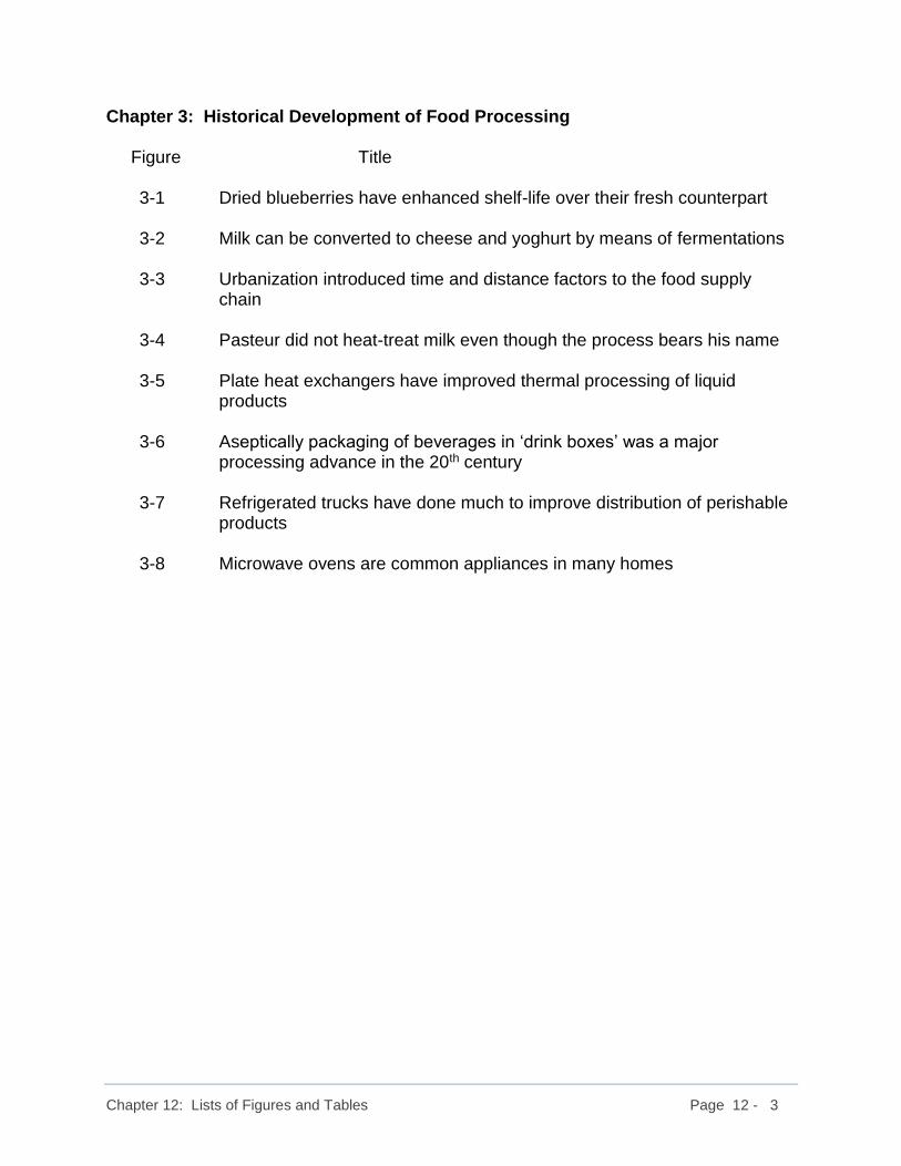
Chapter 12: Lists of Figures and Tables Page 12 - 3
Chapter 3: Historical Development of Food Processing Figure Title
3-1 Dried blueberries have enhanced shelf-life over their fresh counterpart 3-2 Milk can be converted to cheese and yoghurt by means of fermentations 3-3 Urbanization introduced time and distance factors to the food supply
chain 3-4 Pasteur did not heat-treat milk even though the process bears his name 3-5 Plate heat exchangers have improved thermal processing of liquid
products 3-6 Aseptically packaging of beverages in ‘drink boxes’ was a major
processing advance in the 20th century 3-7 Refrigerated trucks have done much to improve distribution of perishable
products 3-8 Microwave ovens are common appliances in many homes
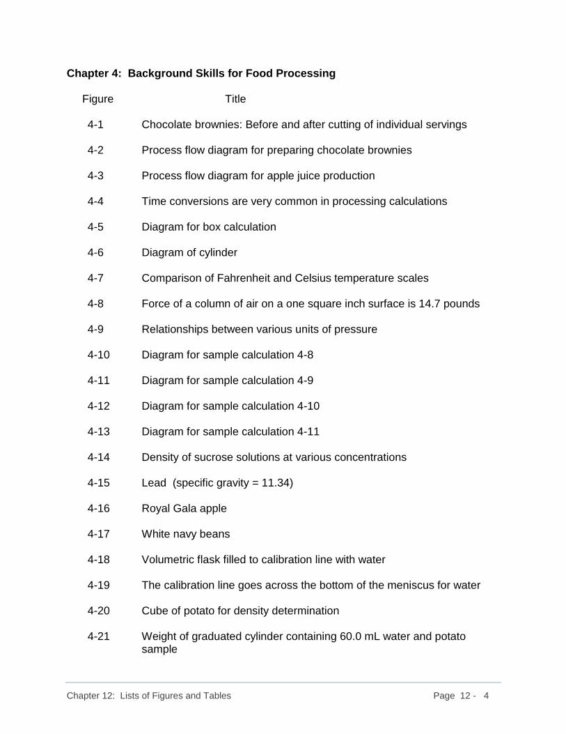
Chapter 12: Lists of Figures and Tables Page 12 - 4
Chapter 4: Background Skills for Food Processing Figure Title
4-1 Chocolate brownies: Before and after cutting of individual servings 4-2 Process flow diagram for preparing chocolate brownies 4-3 Process flow diagram for apple juice production 4-4 Time conversions are very common in processing calculations 4-5 Diagram for box calculation 4-6 Diagram of cylinder 4-7 Comparison of Fahrenheit and Celsius temperature scales 4-8 Force of a column of air on a one square inch surface is 14.7 pounds 4-9 Relationships between various units of pressure 4-10 Diagram for sample calculation 4-8 4-11 Diagram for sample calculation 4-9 4-12 Diagram for sample calculation 4-10 4-13 Diagram for sample calculation 4-11 4-14 Density of sucrose solutions at various concentrations 4-15 Lead (specific gravity = 11.34) 4-16 Royal Gala apple 4-17 White navy beans 4-18 Volumetric flask filled to calibration line with water 4-19 The calibration line goes across the bottom of the meniscus for water 4-20 Cube of potato for density determination 4-21 Weight of graduated cylinder containing 60.0 mL water and potato
sample

Chapter 12: Lists of Figures and Tables Page 12 - 5
4-22 Homemade overflow cup 4-23 Overflow cup set-up prior to running tests 4-24 Potato for overflow cup test 4-25 A slice of potato sinks in water and floats in a 50% sucrose solution due
to their density differences 4-26 Diagram for drying mass balance 4-27 Diagram for orange juice concentration problem

Chapter 12: Lists of Figures and Tables Page 12 - 6
Chapter 5: Heating and Cooling in Food Processing Figure Title
5-1 Mangoes on tree 5-2 Mangoes have a specific heat of approximately 3.550 mL / kg C° 5-3 Chicken meat contains about 74% water by weight 5-4 Tomatoes may contain 94% to 95% water by weight 5-5 Apricots in marketplace 5-6a Preliminary diagram for heating of apricots 5-6b Completed diagram for heating of apricots 5-7 Sides of pork in chilled room 5-8a Preliminary diagram for the freezing of pork chops 5-8b Completed diagram for the heating of pork chops 5-9 Peaches are very susceptible to spoilage after harvesting 5-10 Apple sauce 5-11 Fresh plum before processing 5-12 Fresh strawberries
5-13 It takes 2,257.1 kJ of heat to convert 1.0 kg of vapour at atmospheric pressure
5-14 Autoclave used for sterilizing laboratory equipment 5-15 Using steam as a heat source in a jacketed tank or kettle 5-16 Blueberries before mashing 5-17 Diagram for heating of blueberries 5-18 Diagram for stewing of tomatoes 5-19 Diagram for cooling of stewed tomatoes

Chapter 12: Lists of Figures and Tables Page 12 - 7
5-20 Diagram for heating of tomatoes in sample heat balance 5-21 Diagram for cooling of tomatoes in sample heat balance
Chapter 6: Thermal Processing - Basics Figure Title
6-1 Strawberry jam is thermally processed plus other “hurdles” are present to reduce microbial growth
6-2 Hurdle technology in the preparation of home-made strawberry jam 6-3 Conduction and convection in a heated pot 6-4 Small retort unit for studying thermal processing of canned food products 6-5 Interior of small retort for studying thermal processing of canned food
products 6-6 Heat transfer is accomplished by conduction in thick products and those
with solids such as beef stew 6-7 Unblanched cauliflower will turn brown due to the degradative action of
polyphenol oxidase 6-8 Reaction catalyzed by peroxidase 6-9 Fresh radishes prior to blanching 6-10 Sliced unblanched radishes in hydrogen peroxide solution 6-11 Radish slices were blanched in hot water for 3 minutes 6-12 Inactivation of the peroxidase stops the reaction 6-13 Sliced blanched radishes in hydrogen peroxide solution 6-14 Unblanched turnip slices in a hydrogen peroxide solution 6-15 Slices of blanched turnip in a hydrogen peroxide solution 6-16 Schematic representation of an aseptic process 6-17 Steam injection system for heating liquid products
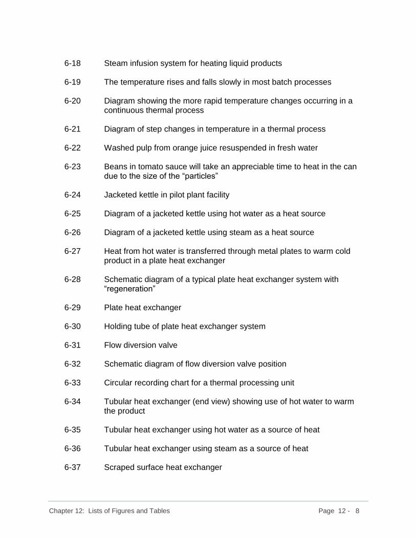
Chapter 12: Lists of Figures and Tables Page 12 - 8
6-18 Steam infusion system for heating liquid products 6-19 The temperature rises and falls slowly in most batch processes 6-20 Diagram showing the more rapid temperature changes occurring in a
continuous thermal process 6-21 Diagram of step changes in temperature in a thermal process 6-22 Washed pulp from orange juice resuspended in fresh water 6-23 Beans in tomato sauce will take an appreciable time to heat in the can
due to the size of the “particles” 6-24 Jacketed kettle in pilot plant facility 6-25 Diagram of a jacketed kettle using hot water as a heat source 6-26 Diagram of a jacketed kettle using steam as a heat source 6-27 Heat from hot water is transferred through metal plates to warm cold
product in a plate heat exchanger 6-28 Schematic diagram of a typical plate heat exchanger system with
“regeneration” 6-29 Plate heat exchanger 6-30 Holding tube of plate heat exchanger system 6-31 Flow diversion valve 6-32 Schematic diagram of flow diversion valve position 6-33 Circular recording chart for a thermal processing unit 6-34 Tubular heat exchanger (end view) showing use of hot water to warm
the product 6-35 Tubular heat exchanger using hot water as a source of heat 6-36 Tubular heat exchanger using steam as a source of heat 6-37 Scraped surface heat exchanger

Chapter 12: Lists of Figures and Tables Page 12 - 9
6-38 End view of a shell and tube heat exchanger using hot water as the heat source
6-39 Side view of shell and tube heat exchanger with hot water as the heat
source 6-40 Side view of shell and tube heat exchanger with steam as the heat
source 6-41 Calcium carbonate (limestone) deposits on heating coils in a kettle 6-42 Partially cleaned coils in kettle and pieces if calcium carbonate removed
from coils

Chapter 12: Lists of Figures and Tables Page 12 - 10
Chapter 7: Thermal Processing – Specialized Calculations Figure Title
7-1 Schematic diagram of set-up for dye injection test 7-2 Hypothetical example of a plot of colour intensity versus retention time
for a dye test 7-3 Schematic diagram of the salt injection set-up for retention time
determination 7-4 Device for injection of salt solution 7-5 Stainless steel tube dimensions 7-6 Graph of microbial population versus time for data presented in Table 7-1 7-7 Graph of the log of microbial population versus time for the data
presented in Table 7-1 7-8 Semi-log plot of microbial population versus time for data from Table 7-1 7-9 Calculation of D-value based on graph shown in Figure 7-8 7-10 Plot of decimal reduction time versus temperature for Geobacillus
stearothermophilus 7-11 Determination of Z-value using graph shown in Figure 7-10 7-12 Plot of log cfu/mL versus time for sample problem

Chapter 12: Lists of Figures and Tables Page 12 - 11
Chapter 8: Basics of Drying Food Materials Figure Title
8-1 Reduction in weight of tomatoes by water removal 8-2 Dehydrated potato flakes offer convenience and portion control 8-3 Plums and grapes can be changed to prunes and raisins by drying 8-4 Removing water from fresh parsley gives dried parsley flakes for
seasoning 8-5 Apples such as this Royal Gala typically contain about 85% water by
weight 8-6 Graph of wet basis moisture versus dry basis moisture 8-7 A closer look at the relationship between wet basis moistures and dry
basis moistures 8-8 Sweet potato with a moisture content of 70% on a wet basis 8-9 Dry powdered starch in plastic tub 8-10 Fresh carrot slices are dried from 86% moisture to 11% moisture 8-11 Diagram of conditions for initial batch of carrots in drying “Case Study” 8-12 Diagram of conditions for second batch of carrots in drying “Case Study” 8-13 Representative food drying curve showing periods of drying 8-14 Dry basis moisture versus time for the drying of hot yellow pepper slices
at 50°C and an air velocity of 0.5 m/s 8-15 Ungelatinized rice kernels leaving a milling process 8-16 The drying properties of hot yellow peppers and fresh oregano are quite
different even when dried under the same conditions 8-17 Fresh cranberries have a waxy outer layer or “cuticle” that prevents
moisture from escaping

Chapter 12: Lists of Figures and Tables Page 12 - 12
8-18 Moisture can travel from the centre to the surface of the sphere with the smaller radius “r” faster than it can in the larger sphere with the radius “R”
8-19 There are three basis shapes considered in drying 8-20 Apple slices dry rapidly due to the porous nature of the apple flesh 8-21 Roma tomatoes tend to have a lower moisture content than other tomato
varieties 8-22 Comparison of specific heats for bananas and strawberries 8-23 The Royal Gala apple has a different texture than the Granny Smith
apple 8-24 This electronic hygrometer indicates the relative humidity of the air at
23°C is 34% and that the air is considered “dry” 8-25 A linear velocity of 0.48 m/s is indicated on this vaned anemometer 8-26 Average daily temperature, relative humidity, and absolute moisture
content of air for Ottawa, Canada 8-27 Colour changes can be exemplified by the effects of toasting on a slice
of white bread 8-28 Maple syrup in an unlabelled bottle 8-29 Warm air removing moisture from a food material 8-30 Excessively hot air creates a dry leathery layer that traps moisture 8-31 Improperly dried apple slices are shown supporting mold growth as
indicated by the red arrows 8-32 Schematic representation of a continuous through circulation dryer 8-33 Diagram of an air distribution plate showing pattern of holes in the metal
plate 8-34 End view of a continuous through circulation dryer showing positioning of
air distribution plate in an updraft zone 8-35 End view of a continuous through circulation dryer showing positioning of
air distribution plate in a downdraft zone

Chapter 12: Lists of Figures and Tables Page 12 - 13
8-36 Schematic diagram of a cabinet dryer 8-37 Schematic diagram of a tunnel dryer 8-38 Schematic diagram of a fluidized bed dryer 8-39 Schematic diagram of a drum dryer 8-40 Schematic diagram of a spray dryer 8-41 Photo of a spray dryer system 8-42 Strips of carrots have been covered in salt to illustrate moisture removal 8-43 Mango slices prior to the start of the osmotic dehydration process 8-44 80 grams of mango slices with approximately 40 grams of sugar 8-45 Mango slices after 8 hours exposure to the sugar at room temperature 8-46 Partially dried mango slices after osmotic dehydration step 8-47 Samples of commercially available dried mango slices with an air-dried
sample on the left and an osmotically dried sample on the right. 8-48 Pictorial representation of the apricot drying process 8-49 Pictorial representation of the apple slice drying process 8-50 Pictorial representation of the parsley drying proces 8-51 Cover of e-book “An Introduction to the Dehydration and Drying of Fruits
and Vegetables”
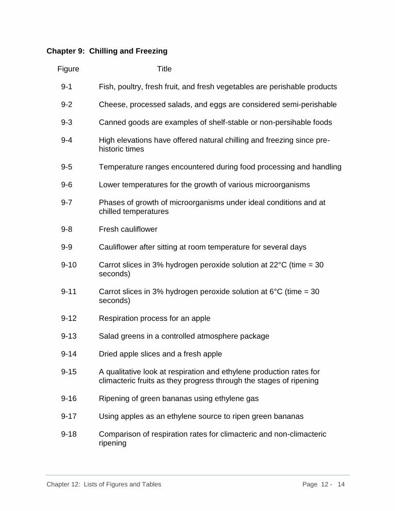
Chapter 12: Lists of Figures and Tables Page 12 - 14
Chapter 9: Chilling and Freezing Figure Title
9-1 Fish, poultry, fresh fruit, and fresh vegetables are perishable products 9-2 Cheese, processed salads, and eggs are considered semi-perishable 9-3 Canned goods are examples of shelf-stable or non-persihable foods 9-4 High elevations have offered natural chilling and freezing since pre-
historic times 9-5 Temperature ranges encountered during food processing and handling 9-6 Lower temperatures for the growth of various microorganisms 9-7 Phases of growth of microorganisms under ideal conditions and at
chilled temperatures 9-8 Fresh cauliflower 9-9 Cauliflower after sitting at room temperature for several days 9-10 Carrot slices in 3% hydrogen peroxide solution at 22°C (time = 30
seconds) 9-11 Carrot slices in 3% hydrogen peroxide solution at 6°C (time = 30
seconds) 9-12 Respiration process for an apple 9-13 Salad greens in a controlled atmosphere package 9-14 Dried apple slices and a fresh apple 9-15 A qualitative look at respiration and ethylene production rates for
climacteric fruits as they progress through the stages of ripening 9-16 Ripening of green bananas using ethylene gas 9-17 Using apples as an ethylene source to ripen green bananas 9-18 Comparison of respiration rates for climacteric and non-climacteric
ripening

Chapter 12: Lists of Figures and Tables Page 12 - 15
9-19 Temperature can have a major impact on the aroma given off by cinnamon and other spices
9-20 Vapour pressure of water as a function of temperature 9-21 A comparison of the vapour pressure of water at 10°C and 20°C 9-22 Firm crisp carrots become flaccid when they lose their moisture 9-23 Fresh baby-cut carrots experience noticeable changes after loss of
surface moisture 9-24 Warm temperatures and moderate relative humidities may be
comfortable for people, but they are not good for storage of most produce
9-25 Waxed sweet green pepper 9-26 Eggplant should not be stored below 7°C 9-27 Potatoes may suffer from cold sweetening if stored improperly 9-28 Bread should not be stored in a refrigerator 9-29 Steps involved in calculating amounts of heat removed in a freezing
process 9-30 Ice cubes floating in water 9-31 Glass jars full of water will crack when frozen due to expansion of the
water 9-32 Broken glass jar after ice has melted 9-33 Temperature versus time graph for freezing of water experiment 9-34 A close-up view of Figure 9-33 showing the “Critical Zone” of ice crystal
growth 9-35 Temperature versus time for freezing of water showing super-cooling 9-36 Comparison of the freezing of water. 30% sucrose solution, and 60%
sucrose solution 9-37 Comparison of the freezing of strawberry jam and pure water

Chapter 12: Lists of Figures and Tables Page 12 - 16
9-38 Comparison of thawing for frozen strawberry jam and ice 9-39 Ice crystal growth in a package of rhubarb stored in a freezer 9-40 A visual representation of how freezing can damage the cells of frozen
foods (Based on Dr. P. Fellows)
Chapter 10: Separation and Concentration Figure Title
10-1 A sieve (or strainer) is an example of separating mixtures of solids and liquids on the basis of particle size
10-2 Sand suspended in moving water will settle when the motion of the water
slows 10-3a A solution of small and large molecules prior to filtration through a
membrane 10-3b Applying pressure forces only solvent and small molecules through the
membrane filter 10-4 A hollow fibre membrane filtration cartridge 10-5 An end view of the membrane cartridge showing the openings of the
potted hollow fibres 10-6 Cut-away of the membrane cartridge showing individual hollow fibres 10-7 Diagram illustrating terms associated with membrane filtration 10-8 A batch membrane filtration process showing return of retentate to the
feed tank 10-9 Diagram of a continuous membrane filtration system 10-10 Diagram to show concept of osmosis with initial conditions and
equilibrium conditions 10-11 Diagram to show concept of reverse osmosis with initial conditions and
after pressure has been applied to the sugar solution

Chapter 12: Lists of Figures and Tables Page 12 - 17
10-12a Microfiltration membranes allow all but particles and colloids to pass through
10-12b Ultrafiltration membranes exclude high molecular weight compounds 10-12c Nanofiltration membranes allow low molecular weight compounds to
pass through 10-12d Hyperfiltration membranes (or reverse osmosis membranes) allow only
water molecules to pass through 10-13 Diagram for sample calculation 10-1 10-14 Schematic diagram of a freeze concentration process 10-15 Diagram for sample calculation 10-2 10-16 Oil layer on water 10-17 Diagram of a solid bowl or “basket” centrifuge 10-18 Diagram of a perforated bowl centrifuge 10-19 Schematic diagram of a horizontal decanter 10-20 Schematic diagram of a desludger 10-21 Diagram of a cyclone separator 10-22 Diagram showing operation of a typical single-effect evaporator 10-23 Removal of calcium ions from solution by ion exchange resin beads 10-24 Diagram of an ion exchange system with regeneration of the column 10-25 Activated carbon from the cartridge of a home water treatment system 10-26 Solvent extraction from a teabag using boiling water as the solvent 10-27 Protein curd formed in soy milk will settle and can be recovered by
filtration 10-28 Schematic diagram of a supercritical solvent extraction process 10-29 Mint oil can be extracted from fresh mint leaves using supercritical
solvent extraction

Chapter 12: Lists of Figures and Tables Page 12 - 18
10-30 Formation of calcium oxalate by the reaction of ammonium oxalate and
calcium chloride 10-31 Reaction between calcium chloride and ammonium oxalate 10-32 Chemical equation for the reaction between calcium chloride and
ammonium oxalate 10-33 Process for solubilizing and precipitating protein

Chapter 12: Lists of Figures and Tables Page 12 - 19
LIST OF TABLES Chapter 4: Background Skills for Food Processing Table Title
4-1 Densities of Various Sucrose Solutions at 20°C 4-2 Density of Water in Various Units (at 20°C) 4-3 Density of Potato Sample from Three Methods
Chapter 5: Heating and Cooling in Food Processing Table Title
5-1 Thermal Properties of Various Food Materials 5-2 Heat Values for Saturated Steam at Various Pressures
Chapter 6: Thermal Processing Basics Table Title
6-1 Time and Temperature Relationships for Milk Pasteurization by Various Methods
6-2 Approximate Times Taken for Particles of Various Sizes to Reach 99%
of Final Temperature
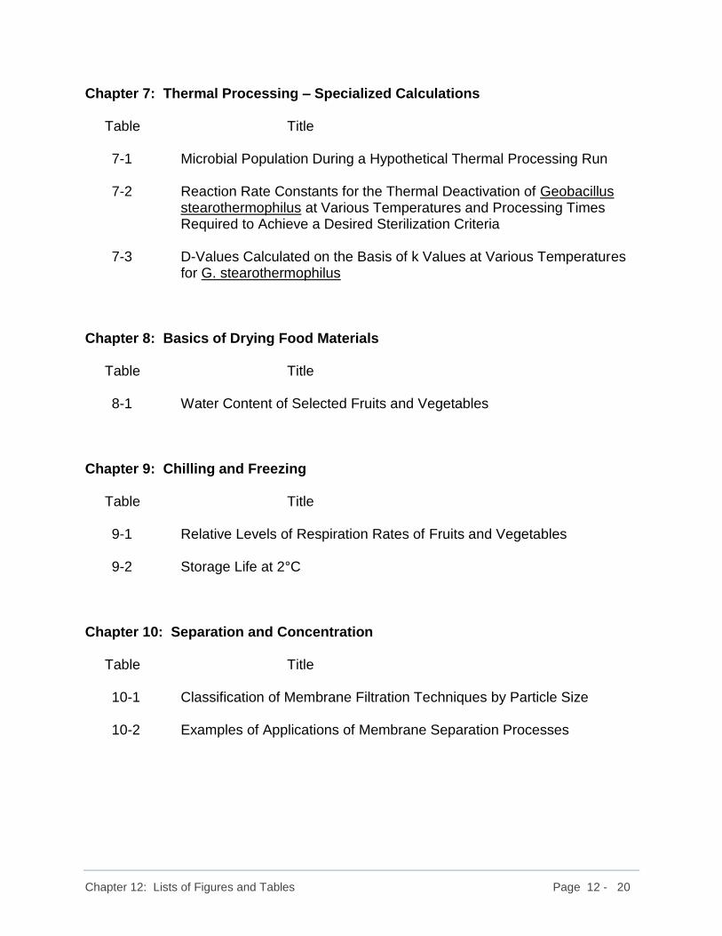
Chapter 12: Lists of Figures and Tables Page 12 - 20
Chapter 7: Thermal Processing – Specialized Calculations Table Title
7-1 Microbial Population During a Hypothetical Thermal Processing Run 7-2 Reaction Rate Constants for the Thermal Deactivation of Geobacillus
stearothermophilus at Various Temperatures and Processing Times Required to Achieve a Desired Sterilization Criteria
7-3 D-Values Calculated on the Basis of k Values at Various Temperatures
for G. stearothermophilus Chapter 8: Basics of Drying Food Materials Table Title
8-1 Water Content of Selected Fruits and Vegetables
Chapter 9: Chilling and Freezing Table Title
9-1 Relative Levels of Respiration Rates of Fruits and Vegetables 9-2 Storage Life at 2°C
Chapter 10: Separation and Concentration Table Title
10-1 Classification of Membrane Filtration Techniques by Particle Size 10-2 Examples of Applications of Membrane Separation Processes