Flutter Analysis of Open-Truss Stiffened Suspension Bridges Using Synthesized Aerodynamic Derivatives

By

Adel Al-Assaf

A dissertation submitted in partial fulfillment of the requirements for the degree of

Doctoral of Philosophy

WASHINGTON STATE UNIVERSITY Department of Civil and Environmental Engineering

DECEMBER 2006

To the Faculty of Washington State University:

The members of the Committee appointed to examine the dissertation of ADEL AL-ASSAF find it satisfactory and recommend that it be accepted.

___________________________________ Chair ___________________________________ ___________________________________

___________________________________ ___________________________________

ii

ACKNOWLEDGMENT

I would like to express my gratitude to my professor in the Washington State

University. Special recognition to Dr. Rafik Itani, Dr. William Cofer, Dr. Cole McDaniel,

Dr. David Stock, Dr. David Pollock and Dr. Balasingam Muhunthan for their help.

This research is made possible by the funding of the United States Federal

Highway Administration and the support of the Washington States Department of

Transportation.

I also would like to thank everyone who helped me during pursuing this research.

iii

Flutter Analysis of Open-Truss Stiffened Suspension Bridges Using Synthesized Aerodynamic Derivatives

Abstract

by Adel Al-Assaf, Ph.D.

Washington State University December 2006

Chair: Rafik Itani

Aerodynamic analysis is of primary consideration in designing long-span bridges.

Theoretical models as well as experimental tools have been developed, which resulted in

Wind tunnel tests becoming the fundamental design tool.

Recent researches focus on alternative methods to assess the wind response of

suspension bridges. These include the computational Fluid Dynamics (CFD) method,

which is based on finite element analysis. Theoretically, this method is capable of solving

different types of fluid-structure-interaction (FSI) problems.

This research discusses the flutter analysis of open-truss stiffened suspension bridges,

with an emphasis on the Second Tacoma Narrows Bridge. The scope is to assess the wind

response of the bridge using analytical tools. The approach suggested here is to

synthesize the wind derivatives based on previous studies of a similar deck configuration.

Then the equation of motion and the synthesized aerodynamic forces are solved to find

the critical wind speed.

iv

In order to conduct an aerodynamic analysis, the frequencies and the mode shapes

of the bridge should be determined. Therefore, a frequency analysis is conducted using a

detailed finite element model. The results are compared with an ambient study of the

bridge, and found to be similar and accurate.

The solution procedure and assumptions of the approach are verified using the

Golden Gate Bridge flutter analyses, where the experimental aerodynamic coefficients of

the bridge are applied in the proposed procedure and compared with the analysis based on

the synthesized coefficients. The results of both cases agree with the results in the

literature. The analysis procedure is then conducted for the Second Tacoma Narrows

Bridge to estimate the critical wind speed is found to be less than the flutter criteria of the

bridge.

v

TABLE OF CONTENTS Chapter 1............................................................................................................................. 1

Introduction......................................................................................................................... 1

1.1 Overview............................................................................................................. 1

1.2 Objectives ........................................................................................................... 4

1.3 Outline................................................................................................................. 4

Chapter 2............................................................................................................................. 7

Theory of Suspension Bridges ............................................................................................ 7

2.1 Introduction............................................................................................................... 7

2.2 Needs and Uses ................................................................................................... 9

2.3 History and Development ................................................................................. 10

Chapter 3........................................................................................................................... 16

Analysis Methods for Cabled Structures .......................................................................... 16

3.1 Introduction............................................................................................................. 16

3.2 Theory of Cable ...................................................................................................... 17

3.2.1 Cable Profile ............................................................................................. 17

3.2.2 Classical Theories ..................................................................................... 19

3.2.3 Finite Element Analysis............................................................................ 21

3.2.3.1 Modeling Issues .................................................................................... 22

3.2.3.2 Finite Element Formulation .................................................................. 25

3.3 Shape-Finding ......................................................................................................... 31

3.4 Frequency Analysis........................................................................................... 32

3.4.1 Eignvalue analysis .................................................................................... 33

3.4.2 Averaged Mechanical Properties .............................................................. 33

vi

Chapter 4........................................................................................................................... 36

Analysis of the Tacoma Narrows Bridge.......................................................................... 36

4.1 Problem................................................................................................................... 36

4.2 Previous Research................................................................................................... 37

4.3 Description and Specifications ............................................................................... 37

4.4 Finite Element Model ............................................................................................. 41

4.4.1 Towers.............................................................................................................. 43

4.4.2 Stiffening Truss................................................................................................ 44

4.4.3 Floor Truss ....................................................................................................... 44

4.4.4 Main Cable....................................................................................................... 45

4.4.5 Hangers ............................................................................................................ 50

4.4.6 Material ............................................................................................................ 51

4.4.7 Section Properties ............................................................................................ 52

4.4.8 Boundary Conditions ....................................................................................... 52

4.4.9 Nonlinear elements .......................................................................................... 53

4.4.10 Load and Mass Estimation............................................................................. 56

4.4.11 Estimation of Mass ........................................................................................ 58

4.5 Frequency Analysis................................................................................................. 59

4.5.1 Ambient Study ................................................................................................. 59

4.5.2 Eigenvalue Analysis......................................................................................... 60

4.5.3 Model Calibration and Analysis ...................................................................... 61

4.6 Results..................................................................................................................... 62

4.7 Discussion ............................................................................................................... 69

vii

Chapter 5........................................................................................................................... 71

Bridge Aeroelasticity ........................................................................................................ 71

5.1 Background............................................................................................................. 71

5.2 Earlier Aeroelasticity Theories ............................................................................... 71

5.3 Early Bridge Aeroelasticity Theories...................................................................... 73

5.4 Wind Forces on Bridges ......................................................................................... 75

5.4.1 Vortex-shedding............................................................................................... 77

5.4.2 Self-induced Forces ......................................................................................... 81

5.4.3 Buffeting .......................................................................................................... 82

5.5 Analytical Models of Flutter................................................................................... 84

5.5.1 Equation of Motion .......................................................................................... 86

5.5.2 Self-induced Forces ......................................................................................... 87

5.5.3 Flutter Derivatives ........................................................................................... 89

5.5.3.1 Extracting Flutter Derivatives................................................................... 91

5.5.3.2 Parametric Analysis .................................................................................. 95

5.5.3.3 Solving for Flutter Condition.................................................................. 105

5.5.3.3.1 Two-Degree-of-Freedom System .................................................... 105

5.5.3.3.2 Verification Problem........................................................................ 111

5.6 Flutter Criteria....................................................................................................... 114

5.7 Estimation of Design Wind Speed........................................................................ 114

Chapter 6......................................................................................................................... 118

Flutter Analysis of the Second Tacoma Narrows Bridge ............................................... 118

6.1 Problem Statement ................................................................................................ 118

viii

6.2 Assumptions and Parameters ................................................................................ 118

6.2.1 Synthesizing Wind Derivative ....................................................................... 119

6.2.2 Verification of the Synthesized Wind Derivative.......................................... 121

6.3 Results................................................................................................................... 122

6.3.1 Critical Flutter Condition............................................................................... 123

6.4 Discussion ............................................................................................................. 124

Chapter 7......................................................................................................................... 127

Conclusions and Recommendations ............................................................................... 127

Appendix A..................................................................................................................... 129

Analysis Results.............................................................................................................. 129

A.1 Second Tacoma Narrows Bridge Frequency Analysis ........................................ 129

Appendix B ..................................................................................................................... 133

MATLAB Programs ....................................................................................................... 133

B.1 Coupling Coefficient ............................................................................................ 133

B.2 Flutter Analysis MATLAB Program.................................................................... 133

Appendix C ..................................................................................................................... 137

C.1 Calculation of Side-Span Profile.......................................................................... 137

1.4 C.2 Derivation of Equations 5.19 coefficients................................................ 137

1.4 C.2 Derivation of Equations 5.19 coefficients................................................ 138

Appendix D..................................................................................................................... 139

Miscellanies Calculations ............................................................................................... 139

D.1 Calculations of the Grate Opening Ratio of Tacoma Narrows Bridge: ............... 139

Appendix E ..................................................................................................................... 140

ix

Parameters for Aeroelasticity.......................................................................................... 140

E.1 Wind Characteristics ............................................................................................ 140

E.1.1 Estimating Wind Parameters ......................................................................... 141

E.2 Flat Plate Aerodynamics....................................................................................... 146

References....................................................................................................................... 148

x

LIST OF FIGURES

Figure 1.1: The Second Tacoma Narrows Bridge .............................................................. 2

Figure 1.2: The open grates of the Second Tacoma Narrows Bridge................................. 3

Figure 2.1: Suspension Bridges Components Chen and Duan (1999)................................ 8

Figure 3.1: Rigid Cable Load............................................................................................ 17

Figure 3.2: Catenary versus parabolic cable profile ......................................................... 19

Figure 3.3: Deflection-load ratio relations among the theories ........................................ 21

Figure 3.4: Catenary Cable Element subjected to nodal displacement............................. 26

Figure 4.1: Section of the Second Tacoma Narrows Bridge Suspended Structure. ........ 38

Figure 4.2: Existing Tacoma Narrows Bridge Elevation View. ....................................... 39

Figure 4.3: The Detailed Finite Element Model of the Tacoma Narrows Bridge ............ 42

Figure 4.4: TNB Main Tower Elev. and Side views......................................................... 43

Figure 4.5: Tacoma Narrows Bridge Floor Truss............................................................. 45

Figure 4.6: Catenary versus parabolic cable profile ......................................................... 47

Figure 4.7: Difference between catenary profile and parabolic profile along the main span

length................................................................................................................................. 49

Figure 4.8: Normalized tension in main cable .................................................................. 49

Figure 4.9: Hanger Force Model....................................................................................... 50

Figure 4.10: Hanger Force ................................................................................................ 51

Figure 4.11: Modeling of Windshoe – top view at deck level.......................................... 55

Figure 4.12: First Mode Period vs Normalized Density ................................................... 56

Figure 4.13: Effect of Eliminating Tower Contribution to Frequency Content ............... 58

Figure 4.14: Mode shapes of Identified Modes ................................................................ 66

xi

Figure 4.15: Normalized modes of vibration.................................................................... 68

Figure 5.1: Grouping of Hangers ...................................................................................... 76

Figure 5.2: Torsional Oscillation of the First Tacoma Narrows Bridge. .......................... 81

Figure 5.3: Flutter forces on a three degrees-of-freedom bridge section.......................... 89

Figure 5.4: NACA-0012-Airfoil test results, for H’s and A’s, by Scanlan and Tomko

(1971)................................................................................................................................ 93

Figure 5.5 : Results for airfoil, Original Tacoma Narrows Bridge Deck, and six ............ 96

Figure 5.6: The aerodynamic derivatives, H1, H3, A1 and A2 for grating-installed

girders, with OR = 40% and α = 0° and α = 3°, Matsumoto et al (2001) ...................... 102

Figure 5.7: The Aerodynamic derivative, A2 for Type 3, Matsumoto et al (2001) ....... 103

Figure 5.8: Lateral flutter derivatives of Akashi-Kaikyo Bridge, Katsuchi et al. (1998)

......................................................................................................................................... 104

Figure 5.9: Flutter analysis for the Golden Gate Bridge................................................. 112

Figure 5.10: Flutter Derivatives of the Golden Gate Bridge Jain et al (1998)................ 113

Figure 6.1: Synthesized flutter derivatives ..................................................................... 121

Figure 6.2: Flutter Analysis of the Golden Gate Bridge using the Flat Plate Theory..... 122

Figure 6.3: Synthesized flutter derivatives ..................................................................... 123

Figure 6.4: Critical Frequencies versus critical reduced wind speed.............................. 123

Figure D.1: The Second Tacoma Narrows Bridge Grates .............................................. 139

xii

LIST OF TABLES

Table 4.1: Comparison between the experimental and the analytical frequencies ........... 63

Table 4.2: Modal Frequency Identification of the TNB ................................................... 64

Table 5.1: Golden Gate Bridge flutter analysis parameters............................................ 113

Table 6.1: Assumptions used to Synthesize flutter coefficients ..................................... 120

Table 6.2: Flutter analysis of the Second Tacoma Narrows Bridge ............................... 124

Table E.1: Air parameters ............................................................................................... 146

xiii

DEDICATION

In memory of my late Mother, my family and all those who took time to help …

xiv

CHAPTER 1 INTRODUCTION 1.1 Overview

Wind is the critical design component of suspension bridges. The failure of the First

Tacoma Narrows Bridge, in November 1940, drew the attention of the impact of wind on

these types of bridges. After the catastrophic failure of the bridge, wind tunnel testing

became a standard method to assess the aerodynamic response of long-span bridges.

Recent researches focus on analytical methods to evaluate the wind response of the

bridge superstructures. The intention is to investigate alternative methods that estimate

the critical wind speed.

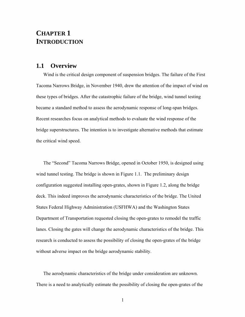
The “Second” Tacoma Narrows Bridge, opened in October 1950, is designed using

wind tunnel testing. The bridge is shown in Figure 1.1. The preliminary design

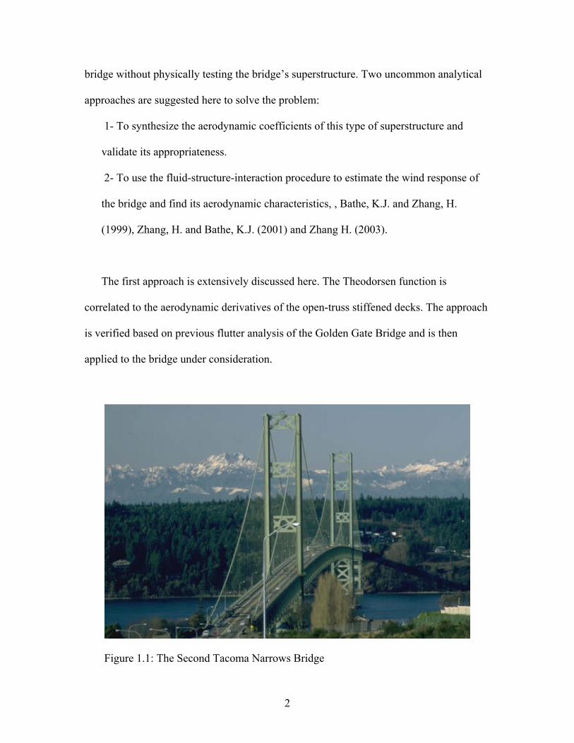
configuration suggested installing open-grates, shown in Figure 1.2, along the bridge

deck. This indeed improves the aerodynamic characteristics of the bridge. The United

States Federal Highway Administration (USFHWA) and the Washington States

Department of Transportation requested closing the open-grates to remodel the traffic

lanes. Closing the gates will change the aerodynamic characteristics of the bridge. This

research is conducted to assess the possibility of closing the open-grates of the bridge

without adverse impact on the bridge aerodynamic stability.

The aerodynamic characteristics of the bridge under consideration are unknown.

There is a need to analytically estimate the possibility of closing the open-grates of the

1

bridge without physically testing the bridge’s superstructure. Two uncommon analytical

approaches are suggested here to solve the problem:

1- To synthesize the aerodynamic coefficients of this type of superstructure and

validate its appropriateness.

2- To use the fluid-structure-interaction procedure to estimate the wind response of

the bridge and find its aerodynamic characteristics, , Bathe, K.J. and Zhang, H.

(1999), Zhang, H. and Bathe, K.J. (2001) and Zhang H. (2003).

The first approach is extensively discussed here. The Theodorsen function is

correlated to the aerodynamic derivatives of the open-truss stiffened decks. The approach

is verified based on previous flutter analysis of the Golden Gate Bridge and is then

applied to the bridge under consideration.

Figure 1.1: The Second Tacoma Narrows Bridge

2

Figure 1.2: The open grates of the Second Tacoma Narrows Bridge

The computational fluid dynamic approach was tested, using ADINA-F. Two bluff

body models were chosen to verify the procedure, namely, a cylinder and an H-shape.

The effort to capture the behavior of the vortex shedding phenomena and the response of

an oscillating cylinder did not lead to any accurate results. Extensive effort was also spent

to obtain the response of an H-shape section in wind, as described in Barriga-Rivera

(1973), using this approach. The oscillatory response was significantly different from

those of the experiments.

Moreover, this approach is found not to be completely robust and convergence is not

always guaranteed. Several issues should be considered to account for the high degree of

nonlinearity in solving the coupled fluid-structure systems. These include some modeling

considerations such as discretization of the domain and the solution time step. The cost of

running a two dimensional model with moderately fine mesh is very expensive. For

3

example, the time required to run one step of the H-shape problem, Barriga-Rivera

(1973), using an Intel Centrino Duo® processor, with two cores 3.2 GHz speed, and

sufficient RAM, is around 4 minutes. The appropriate time step is 1*10-5 second and the

solution should be run for at least 10 seconds. Nevertheless, a three dimensional analysis

is require, which makes the solution infeasible. While this approach was explored

extensively in this research, it was later abandoned because of feasibility, software and

hardware limitations issues.

For any type of aerodynamic analysis, the structural frequencies and the mode shapes

of the bridge are important parameters in the method of analysis. In order to obtain these

parameters a frequency analysis is required. In this research, a detailed finite element

model of the bridge is developed to obtain an accurate estimate of the frequencies content

of the structure.

1.2 Objectives This research develops alternative analytical methods to supplement the wind tunnel

testing, for estimating the critical wind speed of a bridge section with open-truss stiffened

superstructure. The developed approach will be applied to the Second Tacoma Narrows

Bridge to assess the flutter condition of the bridge after closing the existing deck grates.

1.3 Outline This research is divided into two sections:

4

A- The first section discusses the theory of suspension bridges and their behavior.

B- The second investigates the classical flutter analysis and a method to solve the

equation of motion of flutter. In each part the analysis theory is discussed first and

then followed by the bridge’s case study. A brief listing of the coming chapters

and their content is as follows:

Chapter two starts with a historical review of the theory of the suspension bridges,

starting from early attempts in 1800’s and the several bridge catastrophes, to the

evolution of the theory of suspension bridges and the aeroelasticity, and ending with the

contemporary advancements in long-span bridges analysis and construction. The purpose

of the chapter is to give an introductory review of the engineering experience in the

development of suspension bridges.

Chapter 3 includes a discussion of the theory of suspension bridges with the structural

analysis methods of cables. The emphasis is on the catenary cable profile and the

associated modeling issues, such as the methods to evaluate the initial internal forces and

the unstretched profile of cables. A finite element formulation of the three-dimensional

centenary cable is investigated in detail. The chapter is concluded by a discussion of the

frequency analysis of cabled structures.

The frequency analysis of the Second Tacoma Narrows Bridge is discussed in

Chapter 4. The detailed finite element model developed and its structural components are

described. The natural frequencies of the bridge and the mode shapes are compared with

5

previous analytical and experimental frequency analyses. The results are utilized in the

flutter analysis.

Part two of the research starts by a literature review of the previous aerodynamic

theories as discussed in Chapter 5. Various aerodynamic phenomena are described,

highlighting the differences between them and presenting the pertained phenomenon to

the problem under consideration. The pervious studies done on the aerodynamic

coefficients of open-truss stiffened and plate-like superstructures are discussed. The

discussion is then extended to synthesize the flutter derivatives of these types of decks

based on the Theodorsen function. This is useful since the Theodorsen function provides

a closed form solution of the flutter derivatives, as discussed in Appendix E. The

derivation of the equation of motion of flutter condition for a two degrees-of-freedom

system is shown. This chapter is concluded by a case study to verify the derived equation

and the methodology that will be used in the following chapter.

Chapter 6 discusses the flutter analysis of the Second Tacoma Narrows Bridge. The

synthesized flutter derivatives are listed and applied to the current bridge. A previous

study done on the Golden Gate Bridge is used to verify this approach.

6

CHAPTER 2 THEORY OF SUSPENSION BRIDGES

2.1 Introduction

The construction of suspension bridges is well defined and such structures have been

in use for decades. Simple suspension bridges, for use by pedestrians and livestock

transportation, were constructed in the ancient Inca Empire, around year 1200 in South

America, where ropes and wood were used to build bridges. Modern versions of

suspension bridges started with iron chain bridges and then developed to use steel cables.

This type of bridge is naturally aesthetic. Its catenary curve is the essence of its distinct

identity and beauty. The use of suspension bridges emerged due to their enormous

capacity to span long distance.

The advances made in the structural system and analysis methods of suspension

bridges allowed constructing longer spans with better serviceability. Modern bridges are

capable of carrying relatively heavy loads such as vehicles and light rail. The modern

design procedures of suspension bridges are very advanced. However, there are accounts

of success and failure that lead engineers to study the behavior of suspension bridges and

their interaction with nature. The failure of the first Tacoma Narrows Bridge in 1947 is

considered the pivotal point that changed the design of suspension bridges.

Modern suspension bridges are conceptually very similar. Typically, a suspension bridge

consists of main towers that carry the main cables. The cables carry the deck loads via the

7

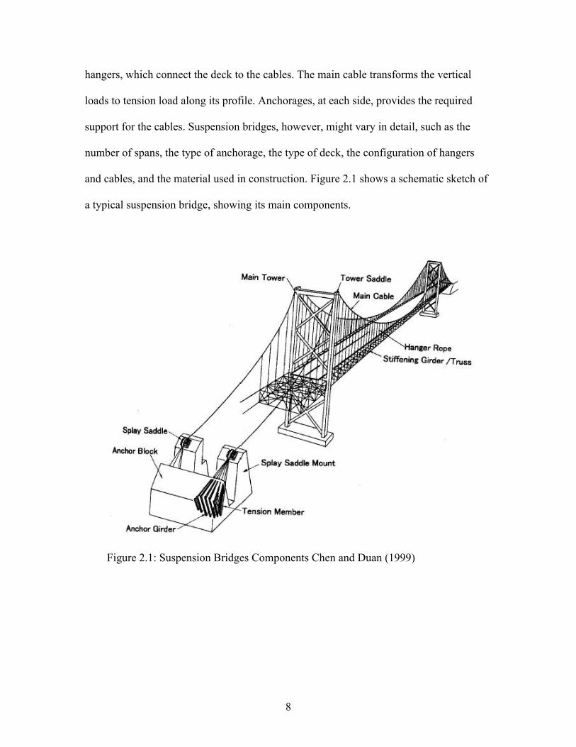
hangers, which connect the deck to the cables. The main cable transforms the vertical

loads to tension load along its profile. Anchorages, at each side, provides the required

support for the cables. Suspension bridges, however, might vary in detail, such as the

number of spans, the type of anchorage, the type of deck, the configuration of hangers

and cables, and the material used in construction. Figure 2.1 shows a schematic sketch of

a typical suspension bridge, showing its main components.

Figure 2.1: Suspension Bridges Components Chen and Duan (1999)

8

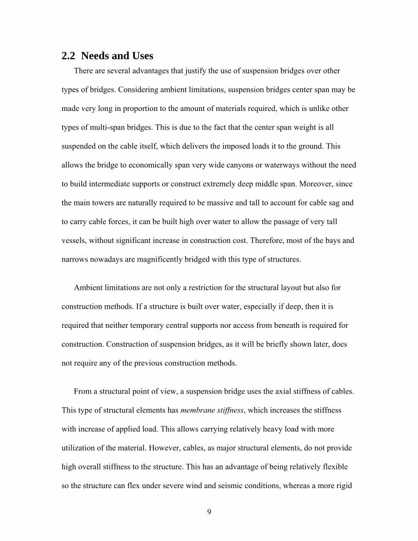
2.2 Needs and Uses There are several advantages that justify the use of suspension bridges over other

types of bridges. Considering ambient limitations, suspension bridges center span may be

made very long in proportion to the amount of materials required, which is unlike other

types of multi-span bridges. This is due to the fact that the center span weight is all

suspended on the cable itself, which delivers the imposed loads it to the ground. This

allows the bridge to economically span very wide canyons or waterways without the need

to build intermediate supports or construct extremely deep middle span. Moreover, since

the main towers are naturally required to be massive and tall to account for cable sag and

to carry cable forces, it can be built high over water to allow the passage of very tall

vessels, without significant increase in construction cost. Therefore, most of the bays and

narrows nowadays are magnificently bridged with this type of structures.

Ambient limitations are not only a restriction for the structural layout but also for

construction methods. If a structure is built over water, especially if deep, then it is

required that neither temporary central supports nor access from beneath is required for

construction. Construction of suspension bridges, as it will be briefly shown later, does

not require any of the previous construction methods.

From a structural point of view, a suspension bridge uses the axial stiffness of cables.

This type of structural elements has membrane stiffness, which increases the stiffness

with increase of applied load. This allows carrying relatively heavy load with more

utilization of the material. However, cables, as major structural elements, do not provide

high overall stiffness to the structure. This has an advantage of being relatively flexible

so the structure can flex under severe wind and seismic conditions, whereas a more rigid

9

bridge would have to be made much stronger and probably much heavier. One

disadvantage of flexible structures is that they may become unusable in strong wind

conditions and may require temporary closure to traffic.

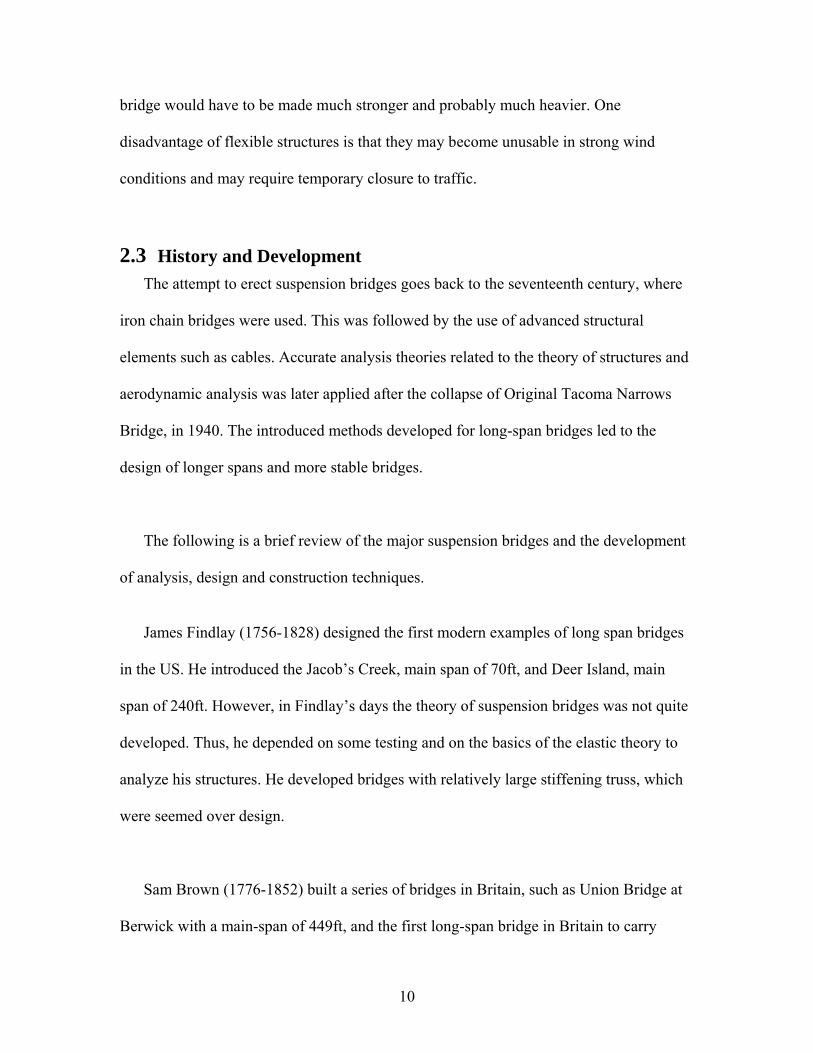
2.3 History and Development

The attempt to erect suspension bridges goes back to the seventeenth century, where

iron chain bridges were used. This was followed by the use of advanced structural

elements such as cables. Accurate analysis theories related to the theory of structures and

aerodynamic analysis was later applied after the collapse of Original Tacoma Narrows

Bridge, in 1940. The introduced methods developed for long-span bridges led to the

design of longer spans and more stable bridges.

The following is a brief review of the major suspension bridges and the development

of analysis, design and construction techniques.

James Findlay (1756-1828) designed the first modern examples of long span bridges

in the US. He introduced the Jacob’s Creek, main span of 70ft, and Deer Island, main

span of 240ft. However, in Findlay’s days the theory of suspension bridges was not quite

developed. Thus, he depended on some testing and on the basics of the elastic theory to

analyze his structures. He developed bridges with relatively large stiffening truss, which

were seemed over design.

Sam Brown (1776-1852) built a series of bridges in Britain, such as Union Bridge at

Berwick with a main-span of 449ft, and the first long-span bridge in Britain to carry

10

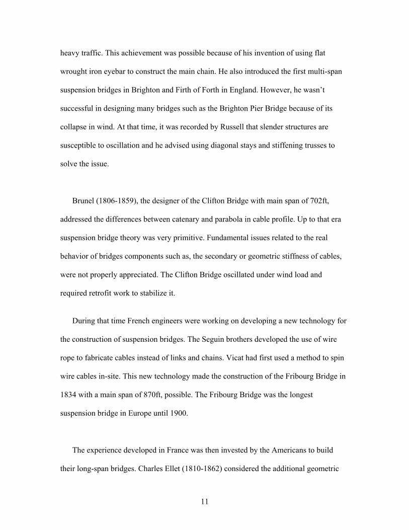
heavy traffic. This achievement was possible because of his invention of using flat

wrought iron eyebar to construct the main chain. He also introduced the first multi-span

suspension bridges in Brighton and Firth of Forth in England. However, he wasn’t

successful in designing many bridges such as the Brighton Pier Bridge because of its

collapse in wind. At that time, it was recorded by Russell that slender structures are

susceptible to oscillation and he advised using diagonal stays and stiffening trusses to

solve the issue.

Brunel (1806-1859), the designer of the Clifton Bridge with main span of 702ft,

addressed the differences between catenary and parabola in cable profile. Up to that era

suspension bridge theory was very primitive. Fundamental issues related to the real

behavior of bridges components such as, the secondary or geometric stiffness of cables,

were not properly appreciated. The Clifton Bridge oscillated under wind load and

required retrofit work to stabilize it.

During that time French engineers were working on developing a new technology for

the construction of suspension bridges. The Seguin brothers developed the use of wire

rope to fabricate cables instead of links and chains. Vicat had first used a method to spin

wire cables in-site. This new technology made the construction of the Fribourg Bridge in

1834 with a main span of 870ft, possible. The Fribourg Bridge was the longest

suspension bridge in Europe until 1900.

The experience developed in France was then invested by the Americans to build

their long-span bridges. Charles Ellet (1810-1862) considered the additional geometric

11

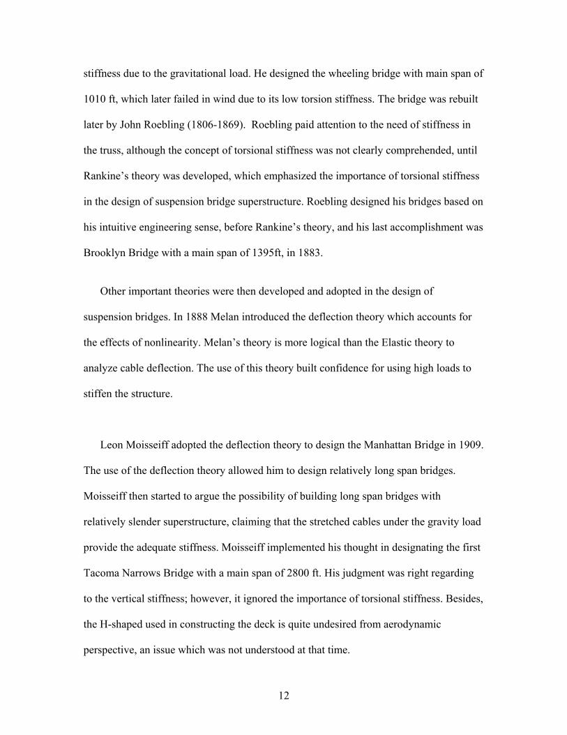
stiffness due to the gravitational load. He designed the wheeling bridge with main span of

1010 ft, which later failed in wind due to its low torsion stiffness. The bridge was rebuilt

later by John Roebling (1806-1869). Roebling paid attention to the need of stiffness in

the truss, although the concept of torsional stiffness was not clearly comprehended, until

Rankine’s theory was developed, which emphasized the importance of torsional stiffness

in the design of suspension bridge superstructure. Roebling designed his bridges based on

his intuitive engineering sense, before Rankine’s theory, and his last accomplishment was

Brooklyn Bridge with a main span of 1395ft, in 1883.

Other important theories were then developed and adopted in the design of

suspension bridges. In 1888 Melan introduced the deflection theory which accounts for

the effects of nonlinearity. Melan’s theory is more logical than the Elastic theory to

analyze cable deflection. The use of this theory built confidence for using high loads to

stiffen the structure.

Leon Moisseiff adopted the deflection theory to design the Manhattan Bridge in 1909.

The use of the deflection theory allowed him to design relatively long span bridges.

Moisseiff then started to argue the possibility of building long span bridges with

relatively slender superstructure, claiming that the stretched cables under the gravity load

provide the adequate stiffness. Moisseiff implemented his thought in designating the first

Tacoma Narrows Bridge with a main span of 2800 ft. His judgment was right regarding

to the vertical stiffness; however, it ignored the importance of torsional stiffness. Besides,

the H-shaped used in constructing the deck is quite undesired from aerodynamic

perspective, an issue which was not understood at that time.

12

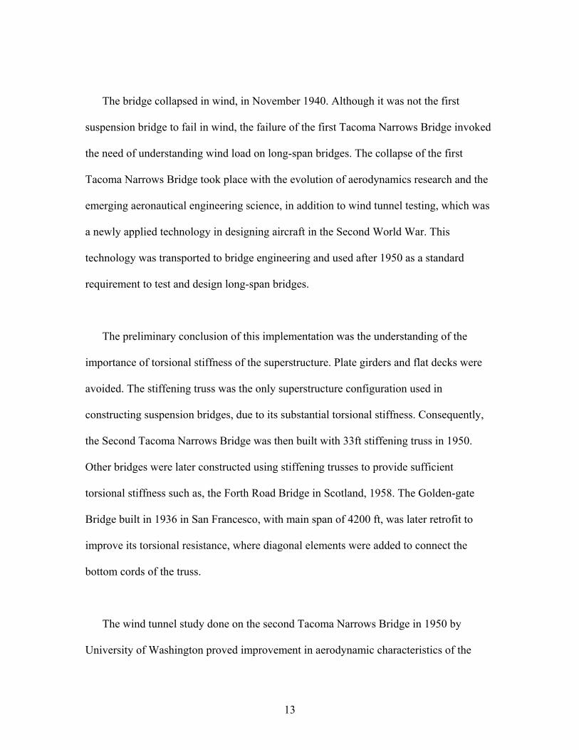
The bridge collapsed in wind, in November 1940. Although it was not the first

suspension bridge to fail in wind, the failure of the first Tacoma Narrows Bridge invoked

the need of understanding wind load on long-span bridges. The collapse of the first

Tacoma Narrows Bridge took place with the evolution of aerodynamics research and the

emerging aeronautical engineering science, in addition to wind tunnel testing, which was

a newly applied technology in designing aircraft in the Second World War. This

technology was transported to bridge engineering and used after 1950 as a standard

requirement to test and design long-span bridges.

The preliminary conclusion of this implementation was the understanding of the

importance of torsional stiffness of the superstructure. Plate girders and flat decks were

avoided. The stiffening truss was the only superstructure configuration used in

constructing suspension bridges, due to its substantial torsional stiffness. Consequently,

the Second Tacoma Narrows Bridge was then built with 33ft stiffening truss in 1950.

Other bridges were later constructed using stiffening trusses to provide sufficient

torsional stiffness such as, the Forth Road Bridge in Scotland, 1958. The Golden-gate

Bridge built in 1936 in San Francesco, with main span of 4200 ft, was later retrofit to

improve its torsional resistance, where diagonal elements were added to connect the

bottom cords of the truss.

The wind tunnel study done on the second Tacoma Narrows Bridge in 1950 by

University of Washington proved improvement in aerodynamic characteristics of the

13

bridge when open-grates were used along the superstructure. Open-grates became the

solution to improve deck aerodynamics. Another improvement of the truss aerodynamics

was the introduction of a vertical stabilizer running longitudinally in the deck. This

improvement was recently applied in the Great Belt Bridge and the Akashi-Kaikyo

Bridge.

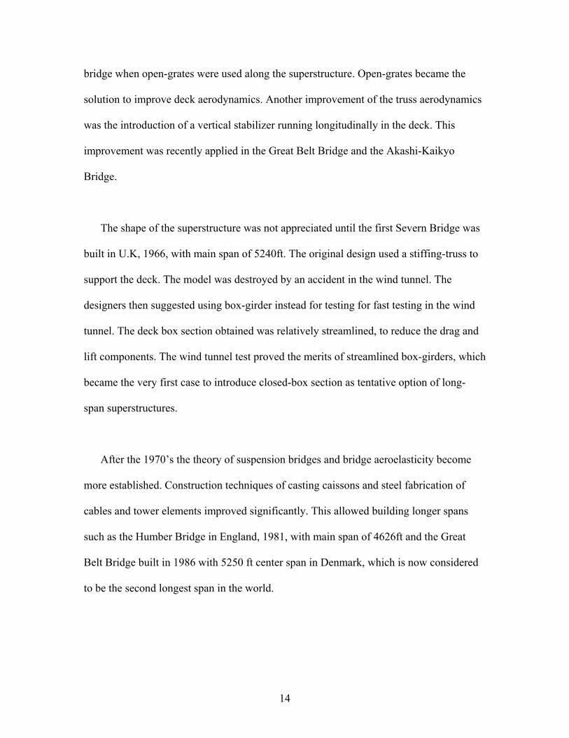
The shape of the superstructure was not appreciated until the first Severn Bridge was

built in U.K, 1966, with main span of 5240ft. The original design used a stiffing-truss to

support the deck. The model was destroyed by an accident in the wind tunnel. The

designers then suggested using box-girder instead for testing for fast testing in the wind

tunnel. The deck box section obtained was relatively streamlined, to reduce the drag and

lift components. The wind tunnel test proved the merits of streamlined box-girders, which

became the very first case to introduce closed-box section as tentative option of long-

span superstructures.

After the 1970’s the theory of suspension bridges and bridge aeroelasticity become

more established. Construction techniques of casting caissons and steel fabrication of

cables and tower elements improved significantly. This allowed building longer spans

such as the Humber Bridge in England, 1981, with main span of 4626ft and the Great

Belt Bridge built in 1986 with 5250 ft center span in Denmark, which is now considered

to be the second longest span in the world.

14

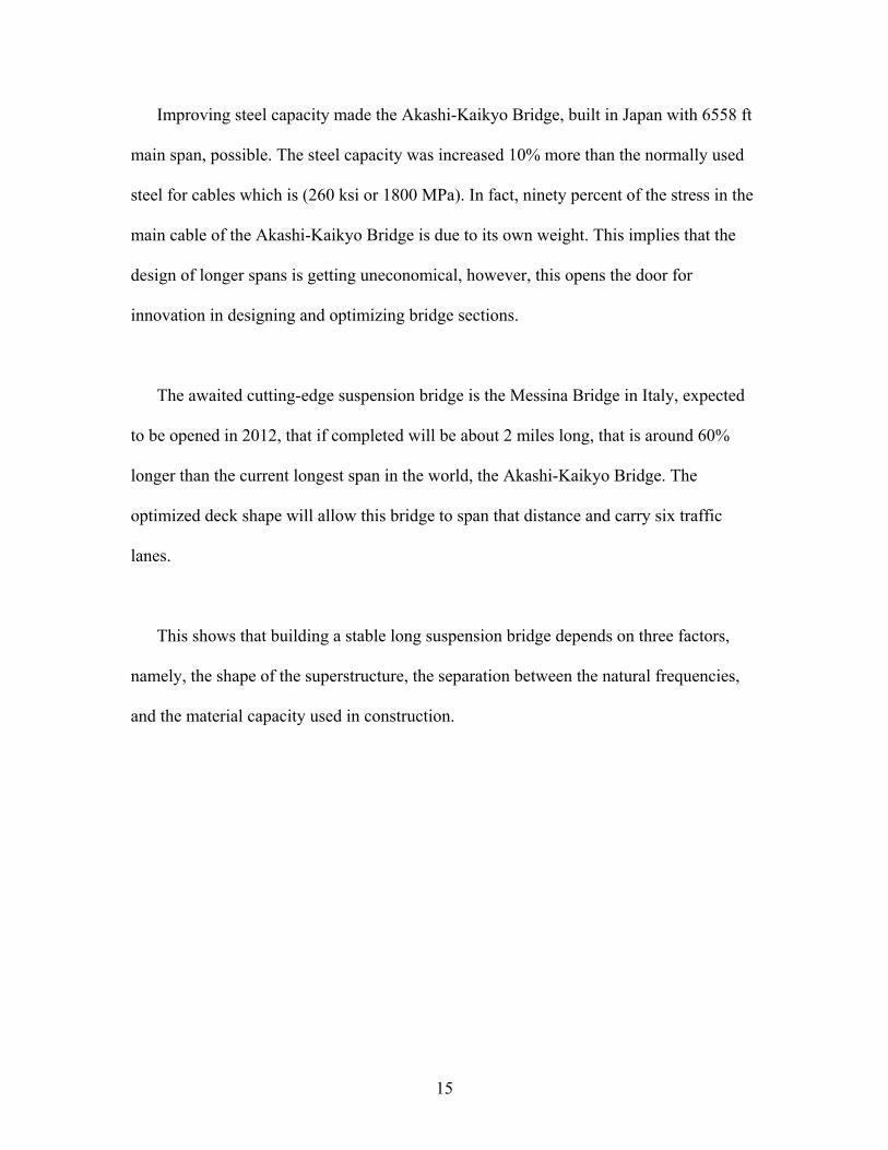
Improving steel capacity made the Akashi-Kaikyo Bridge, built in Japan with 6558 ft

main span, possible. The steel capacity was increased 10% more than the normally used

steel for cables which is (260 ksi or 1800 MPa). In fact, ninety percent of the stress in the

main cable of the Akashi-Kaikyo Bridge is due to its own weight. This implies that the

design of longer spans is getting uneconomical, however, this opens the door for

innovation in designing and optimizing bridge sections.

The awaited cutting-edge suspension bridge is the Messina Bridge in Italy, expected

to be opened in 2012, that if completed will be about 2 miles long, that is around 60%

longer than the current longest span in the world, the Akashi-Kaikyo Bridge. The

optimized deck shape will allow this bridge to span that distance and carry six traffic

lanes.

This shows that building a stable long suspension bridge depends on three factors,

namely, the shape of the superstructure, the separation between the natural frequencies,

and the material capacity used in construction.

15

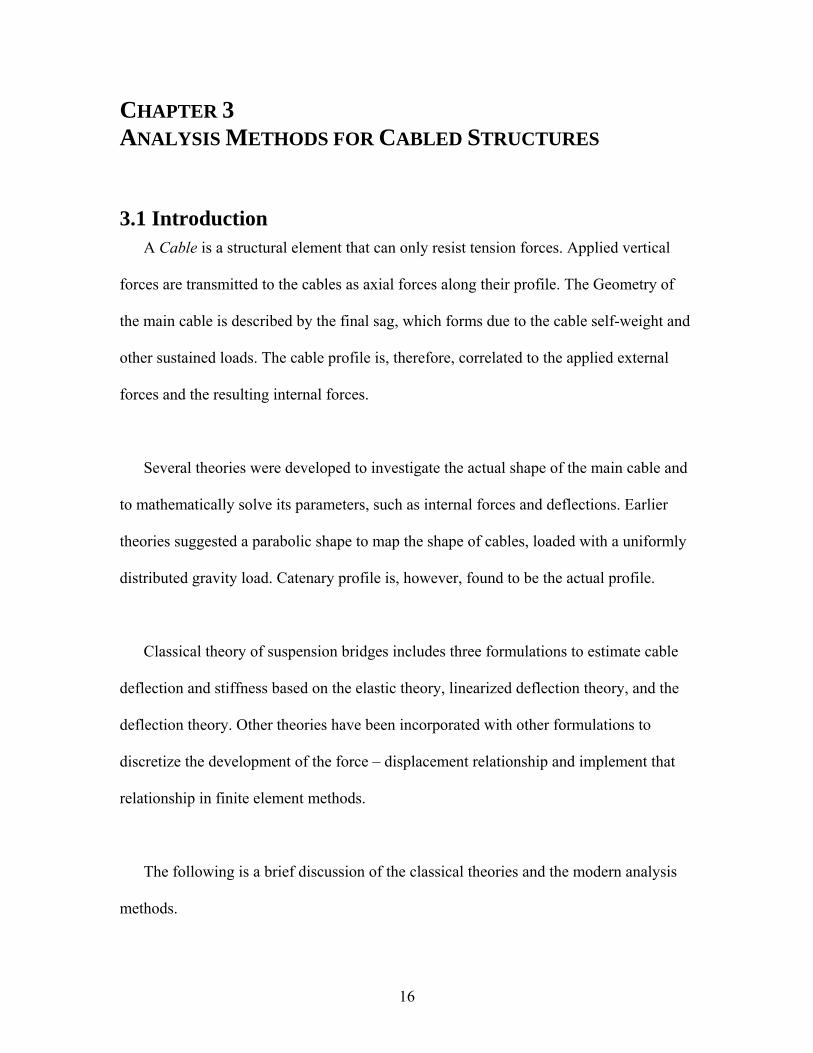
CHAPTER 3 ANALYSIS METHODS FOR CABLED STRUCTURES 3.1 Introduction

A Cable is a structural element that can only resist tension forces. Applied vertical

forces are transmitted to the cables as axial forces along their profile. The Geometry of

the main cable is described by the final sag, which forms due to the cable self-weight and

other sustained loads. The cable profile is, therefore, correlated to the applied external

forces and the resulting internal forces.

Several theories were developed to investigate the actual shape of the main cable and

to mathematically solve its parameters, such as internal forces and deflections. Earlier

theories suggested a parabolic shape to map the shape of cables, loaded with a uniformly

distributed gravity load. Catenary profile is, however, found to be the actual profile.

Classical theory of suspension bridges includes three formulations to estimate cable

deflection and stiffness based on the elastic theory, linearized deflection theory, and the

deflection theory. Other theories have been incorporated with other formulations to

discretize the development of the force – displacement relationship and implement that

relationship in finite element methods.

The following is a brief discussion of the classical theories and the modern analysis

methods.

16

3.2 Theory of Cable

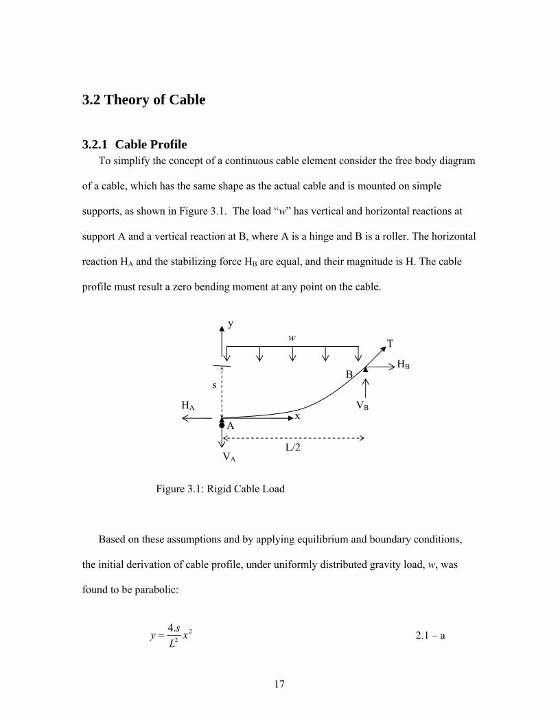
3.2.1 Cable Profile To simplify the concept of a continuous cable element consider the free body diagram

of a cable, which has the same shape as the actual cable and is mounted on simple

supports, as shown in Figure 3.1. The load “w” has vertical and horizontal reactions at

support A and a vertical reaction at B, where A is a hinge and B is a roller. The horizontal

reaction HA and the stabilizing force HB are equal, and their magnitude is H. The cable

profile must result a zero bending moment at any point on the cable.

Figure 3.1: Rigid Cable Load

Based on these assumptions and by applying equilibrium and boundary conditions,

the initial derivation of cable profile, under uniformly distributed gravity load, w, was

found to be parabolic:

2

2

.4 xL

sy = 2.1 – a

VA

VB

A

B HB

s

HA

w y

T

x

L/2

17

sLwH.8. 2

= 2.1 – b

22 2.42

.⎟⎠⎞

⎜⎝⎛+⎟

⎠⎞

⎜⎝⎛=

Lx

sLLwT 2.1 – c

where, s is the sag, L is the span length of the parabola, w is the total gravity load

distributed uniformly allover the cable length, and x and y are the horizontal and vertical

distances, measured according to the reference point shown in Figure 3.2.

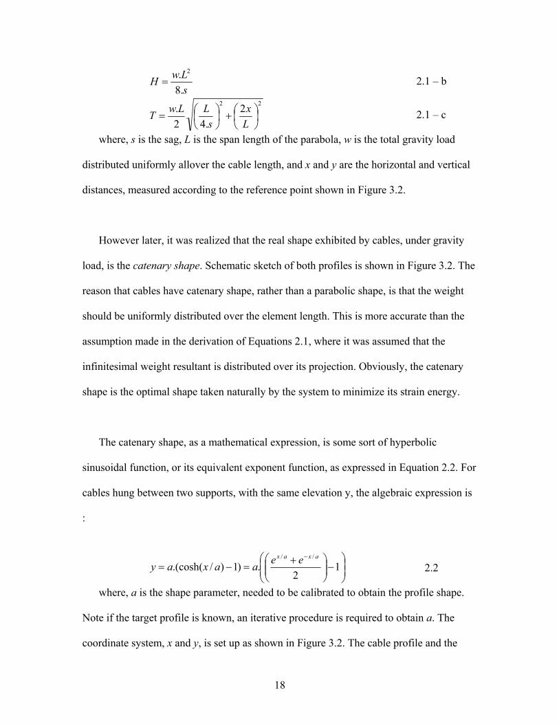
However later, it was realized that the real shape exhibited by cables, under gravity

load, is the catenary shape. Schematic sketch of both profiles is shown in Figure 3.2. The

reason that cables have catenary shape, rather than a parabolic shape, is that the weight

should be uniformly distributed over the element length. This is more accurate than the

assumption made in the derivation of Equations 2.1, where it was assumed that the

infinitesimal weight resultant is distributed over its projection. Obviously, the catenary

shape is the optimal shape taken naturally by the system to minimize its strain energy.

The catenary shape, as a mathematical expression, is some sort of hyperbolic

sinusoidal function, or its equivalent exponent function, as expressed in Equation 2.2. For

cables hung between two supports, with the same elevation y, the algebraic expression is

:

⎟⎟⎠

⎞⎜⎜⎝

⎛−⎟⎟

⎠

⎞⎜⎜⎝

⎛ +=−=

−

12

.)1)/.(cosh(// axax eeaaxay 2.2

where, a is the shape parameter, needed to be calibrated to obtain the profile shape.

Note if the target profile is known, an iterative procedure is required to obtain a. The

coordinate system, x and y, is set up as shown in Figure 3.2. The cable profile and the

18

internal forces of the Second Tacoma Narrows Bridge are discussed in Chapter 3,

showing the difference between both profile shapes.

Parabolic

Figure 3.2: Catenary versus parabolic cable profile

3.2.2 Classical Theories The first theory of suspension bridges was published by Rankine in 1858. The theory

assumptions were made based on an abstraction of suspension bridges system, that is, a

bridge comprising a straight and horizontal roadway slung from suspension cables and

stiffened in some measures by longitudinal girders at the road level. The theory assumes

that under total dead load the cable is parabolic and the stiffening girder is unstressed.

Any partial or concentrated load on a platform must, by means of the girder, be

transmitted to the “chain” in such a manner as to be uniformly distributed on the chain.

Rankine’s idea implies that the tension in the hangers should be the same under any

type of loading, and that is, in a free-body diagram of the girder the hanger forces are

assumed to be a uniformly distributed load along the span and acting upward. To achieve

this assumption the girder should be sufficiently deep. This might be economic and

Catenary y L/2

s x

19

feasible for relatively short spans, that is, a few hundred feet long; but would be

uneconomic for relatively longer spans.

The above assumptions were, mainly, applied to two well-known theories, the elastic

theory and the deflection theory. The difference between them is whether cable deflection

resulting from live load is considered. The bending moment equation along the stiffening

girder and after applying the live load is evaluated and employed in the strain energy

equations to derive the force – displacement relationship along the bridge span. This

difference leads to a major discrepancy in both theories.

The inclusion of deformation in the deflection theory yields two main differences

from the elastic theory. The first is that it reduces the bending moment of the stiffening

girder. The second is that the derivation will be nonlinear and recursive, that is, the

parameters of the strain energy equation is a function of its results. The nonlinearity of

the deflection method makes the principle of superposition and influence line analysis

inapplicable. Therefore, another theory was introduced to linearize the deflection theory

by assuming that the ratio of the live load to the dead load is very small. This implies that

the deflection is constant and is due to the dead load only.

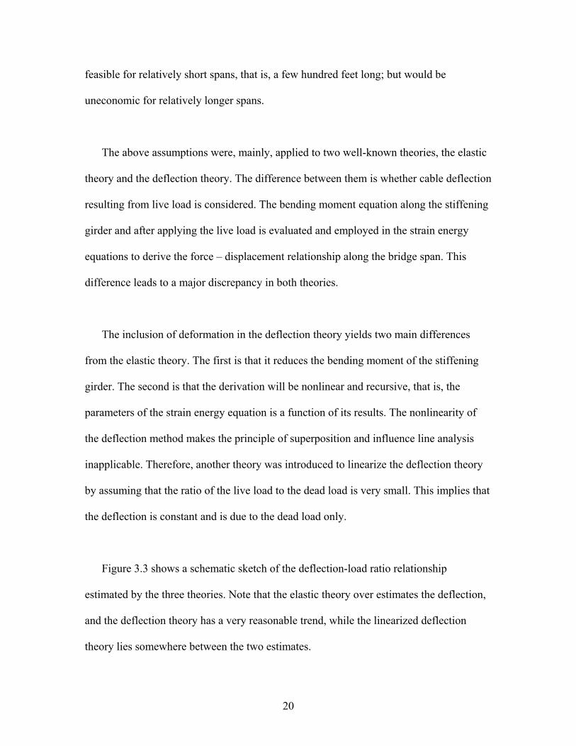
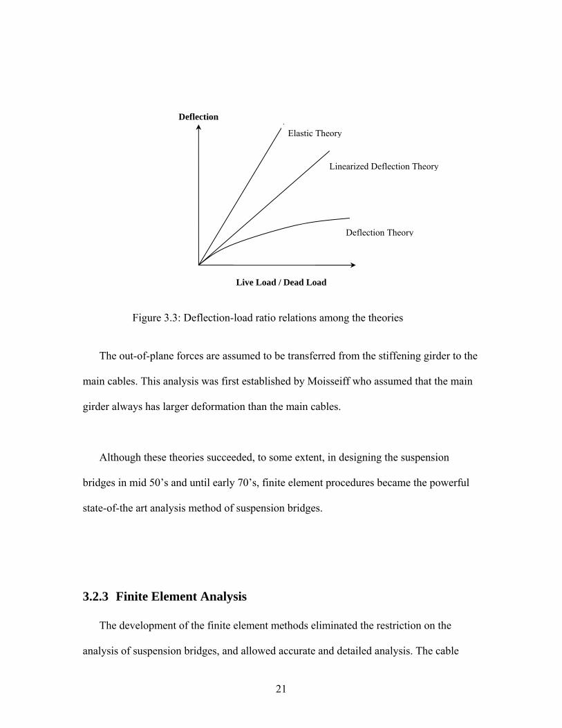
Figure 3.3 shows a schematic sketch of the deflection-load ratio relationship

estimated by the three theories. Note that the elastic theory over estimates the deflection,

and the deflection theory has a very reasonable trend, while the linearized deflection

theory lies somewhere between the two estimates.

20

Deflection

Figure 3.3: Deflection-load ratio relations among the theories

The out-of-plane forces are assumed to be transferred from the stiffening girder to the

main cables. This analysis was first established by Moisseiff who assumed that the main

girder always has larger deformation than the main cables.

Although these theories succeeded, to some extent, in designing the suspension

bridges in mid 50’s and until early 70’s, finite element procedures became the powerful

state-of-the art analysis method of suspension bridges.

3.2.3 Finite Element Analysis

The development of the finite element methods eliminated the restriction on the

analysis of suspension bridges, and allowed accurate and detailed analysis. The cable

Linearized Deflection Theory

Elastic Theory

Deflection Theory

Live Load / Dead Load

21

element is no longer assumed as a continuous element, the hangers are included as

discrete entities, even the elements of the stiffening girders are modeled explicitly, three-

dimensional analysis is possible, and all geometric and material variations along the span

are accountable.

3.2.3.1 Modeling Issues

Modeling of suspension bridges can be done using a combination of different types of

finite element modules and different analysis procedures. This depends on the type of the

structural element being modeled, such as beam, cable or shell, the elasticity

assumptions, the type of analysis required, such as dynamic, static or P-∆ analysis, and

the stage of construction being modeled, such as, the initial construction stages or the

final as-built analyses. The following discussion considers linear elastic finite element

analysis of suspension bridges with an open-truss stiffening girder at the final, as-built,

configuration. The discussion is mainly made to develop a finite element model to

estimate the dynamic response of a bridge.

The level of modeling sophistication varies from a very simplified spine model,

where the superstructure and the towers are lumped in discrete beam elements, called

spine elements, to complete detailed finite element models, where every single element is

explicitly modeled. The first approach was the most desirable in the early 70’s and mid

80’s, when the computer resources were very limited. A detailed model, however, is

possible nowadays. A detailed finite element model of the Second Tacoma Narrows

Bridge is discussed in the coming chapter. The frequency analysis results are compared

22

with frequencies obtained experimentally and with frequencies obtained from a previous

study, done with less detail.

Detailed models are more accurate than condensed models. Detailed models are more

capable of estimating stiffness and mass distributions along the structure. Spine models

should be avoided in relatively flexible superstructures. That is because the estimation of

the torsional stiffness of a spine element base on the cross sectional properties of the

original configuration, is usually inaccurate especially when a segment of a space truss is

being condensed. A magnification factor of the computed properties is usually applied to

calibrate the element response. Another issue associated with the use of spine models is

the difficulty of modeling the location of the center of mass and the center of rigidly of

the element, which might affect the accuracy of a dynamic analysis.

Beam elements or truss elements can be used to model stiffening-truss girders. This

depends on the type of joints connecting the elements. It is acceptable to model a truss

using beam elements provided that all loads and masses are lumped at the joint, the

stiffness of the elements is relatively close to one another, the bending stiffness of each

element is relatively small compared to its axial stiffness and compared to the total

bending stiffness of the truss, and the angles between the elements are not very large, less

than 130°.

For elastic analysis, the conventional beam element, derived based on beam theory, is

appropriate. The beam element could be used to model the superstructure elements and

23

the towers. Since the tower legs are usually substantial in dimensions, offsets or rigid

links might be used to model the rigid joint effect at element intersections.

Modeling of cables requires special attention to two main issues. The first is the

formulation of the element, and the second is the initial condition of the element. Cables,

as described earlier, have unique nonlinear force – displacement behavior. The stiffness

matrix of a cable element should be formulated accordingly, that is, to account for the

geometric nonlinearity. The different ways to formulate a cable element are described in

the coming section.

Since the stiffness of a cable element is a function of its internal forces, initial internal

forces should be calculated. These forces are due to the deflection due to the self-weight

of the cable and/or the total sustained load. The initial profile of a simply supported

cable, under its own weight, will sag to its final or target profile due to the application of

the sustained gravity loads. A shape-finding process is usually required to estimate the

final shape of a cable and its associated internal forces. A brief discussion of this process

is conducted in this chapter.

It is definite that the static analysis procedure of suspension bridges is nonlinear,

where iterative procedures should be conducted to reach equilibrium at the final sag.

Frequency analysis is usually conducted based on linear Eigenvalue analysis, where the

initial conditions assigned are used in stiffness estimation. However, due to the

considerable difference in the flexibility of the bridge components, such as the main cable

24

and the superstructure, the Ritz method is strongly recommended to eliminate local

modes of vibrations, Chopra (2001).

3.2.3.2 Finite Element Formulation

The formulation of a cable element could be done in two different ways. The first one

is based on the equivalent truss element, where the stiffness is derived by minimizing the

strain energy of a line element, assuming linear shape function and non-linear second

order strain function, Przemieniecki (1968). The result is a stiffness matrix which is

function of the external deflections, i.e., the internal force in the element. The local

tangent stiffness matrix of the equivalent truss element is:

32

312Lw

TL

EAKt += 2.3

where, A is the cable cross section area, E is the modulus of elasticity, L is the length.

The first term in the above equation is the elastic stiffness and the second term is the

geometric stiffness due to sag. Elements developed based on this formulation are called

linear cable elements.

These types of elements are suitable to model straight tendons or cables with high

tension, where the cable profile is almost linear. A cable with large sag or vertical

deflection has a catenary profile, and thus an element formulated based on a linear shape

function is not the best modeling choice.

For cables with large sag or large vertical deformation a catenary element should be

used. The fundamentals of this element are discussed in Irvine (1981). Kim and Lee

25

(2001) briefly discussed the derivation of a two-dimensional catenary cable. The

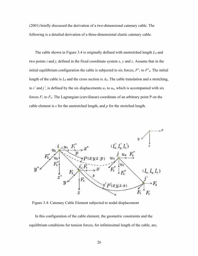
following is a detailed derivation of a three-dimensional elastic catenary cable.

The cable shown in Figure 3.4 is originally defined with unstretched length L0 and

two points i and j, defined in the fixed coordinate system x, y and z. Assume that in the

initial equilibrium configuration the cable is subjected to six forces, Fo1 to Fo

6. The initial

length of the cable is L0 and the cross section is A0. The cable translation and a stretching,

to i’ and j’, is defined by the six displacements u1 to u6, which is accompanied with six

forces F1 to F6. The Lagrangian (curvilinear) coordinate of an arbitrary point P on the

cable element is s for the unstretched length, and p for the stretched length.

Figure 3.4: Catenary Cable Element subjected to nodal displacement

In this configuration of the cable element, the geometric constraints and the

equilibrium conditions for tension forces, for infinitesimal length of the cable, are,

26

1222

=⎟⎟⎠

⎞⎜⎜⎝

⎛+⎟⎟

⎠

⎞⎜⎜⎝

⎛+⎟⎟

⎠

⎞⎜⎜⎝

⎛dpdz

dpdy

dpdx 2.4

wsFdpdzT

FdpdyT

FdpdxT

−−=⎟⎟⎠

⎞⎜⎜⎝

⎛

−=⎟⎟⎠

⎞⎜⎜⎝

⎛

−=⎟⎟⎠

⎞⎜⎜⎝

⎛

3

2

1

2.5

where, w is the weight of the cable per unit length. This implies the following,

( )( ) 2/1223

22

21 wsFFFT +++= 2.6

The nodal forces equilibrium and displacement compatibility conditions are,

( )( )( )36

0

250

140

036

25

14

uull

uull

uull

wLFFFFFF

zz

yy

xx

−+=

−+=

−+=

−−=−=−=

2.7

The relationships between the undeformed Lagrangian coordinate s and Cartesian

coordinate are,

∫

∫

∫

=

=

=

dsdsdzsz

dsdsdysy

dsdsdxsx

)(

)(

)(

2.8

A constitutive relation that is a mathematically consistent expression of Hooke’s law

is

⎟⎠⎞

⎜⎝⎛ −= 10 ds

dpEAT 2.9

27

Therefore, from Equations 2.5 and 2.9, the following could be derived,

⎟⎟⎠

⎞⎜⎜⎝

⎛+−=−== 1

0

11

EAT

TF

dsdp

TF

dsdp

dpdx

dsdx

⎟⎟⎠

⎞⎜⎜⎝

⎛+−=−== 1

0

22

EAT

TF

dsdp

TF

dsdp

dpdy

dsdy

( ) ( )⎟⎟⎠

⎞⎜⎜⎝

⎛+

−−=

−−== 1

0

33

EAT

TwsF

dsdp

TwsF

dsdp

dpdx

dsdx

2.10

Substituting the Equations 2.10 in 2.8 and integration with respect to s gives,

⎥⎦

⎤⎢⎣

⎡⎟⎟⎠

⎞⎜⎜⎝

⎛ +−⎟⎟

⎠

⎞⎜⎜⎝

⎛−−= −−

1

31

1

311

0

1)(F

wsFSinhFFSinh

wF

EAsFsx 2.11

which are equivalent to,

[ ]TFTwsFwF

EAsFsx +−++−−= 33

1

0

1 lnln)( 2.12

Working out for the other directions,

[ ]TFTwsFwF

EAsFsy +−++−−= 33

2

0

2 lnln)( 2.13

[ ]2/123

22

21

0

2

0

3 12

.)( FFFTwEA

swEA

sFsz ++−−−−= 2.14

The boundary conditions at the cable ends are,

x = 0, y = 0, z = 0, p = 0 at s = 0 x = lx, y = ly, z = lz, p = L at s = L0

2.15

Applying the boundary conditions gives the following,

[ ]TFTwLFwF

EALFlx +−++−−= 303

1

0

01 lnln

[ ]TFTwLFwF

EALFly +−++−−= 303

2

0

02 lnln or i

[ ]2/123

22

21

0

20

0

03 12

FFFTwEA

wLEA

LFlz ++−−−−=

( ) 2/1203

22

21 wLFFFT +++=

2.16

28

To implement the finite element procedure, the nodal forces have to be expressed

with respect to the global nodal displacements of the element. Note that the above

nonlinear relations satisfy this requirement. Applying an incremental procedure using the

first order Taylor expansion, with respect to the unknowns F1, F2, and F3 the following

expression is obtained,

33

12

2

11

1

11 dF

FldF

FldF

Fldl

∂∂

+∂∂

+∂∂

=

33

22

2

21

1

22 dF

FldF

FldF

Fldl

∂∂

+∂∂

+∂∂

=

33

32

2

31

1

33 dF

FldF

FldF

Fldl

∂∂

+∂∂

+∂∂

=

2.17

Or in matrix form

⎪⎭

⎪⎬

⎫

⎪⎩

⎪⎨

⎧=

⎪⎭

⎪⎬

⎫

⎪⎩

⎪⎨

⎧

3

2

1

3

2

1

dFdFdF

Fdldldl

2.18

Where F is the nodal flexibility matrix, defined as follows:

⎪⎭

⎪⎬

⎫

⎪⎩

⎪⎨

⎧=

⎪⎪⎪

⎭

⎪⎪⎪

⎬

⎫

⎪⎪⎪

⎩

⎪⎪⎪

⎨

⎧

∂∂

∂∂

∂∂

∂∂

∂∂

∂∂

∂∂

∂∂

∂∂

=

333231

232221

131211

3

3

2

3

1

3

3

2

2

2

1

2

3

1

2

1

1

1

fffffffff

Fl

Fl

Fl

Fl

Fl

Fl

Fl

Fl

Fl

F

2.19

The forces are equal to

⎪⎭

⎪⎬

⎫

⎪⎩

⎪⎨

⎧=

⎪⎭

⎪⎬

⎫

⎪⎩

⎪⎨

⎧

3

2

1

3

2

1

dldldl

KdFdFdF

, 1−= FK 2.20

where K is the nodal stiffness matrix.

29

The components of the flexibility matrix in the above equations are,

[ ]

( ) ⎥⎦

⎤⎢⎣

⎡+

−++

−

+−++−−=

AFATwLFTwF

AFTwLFwEA

Lf

32

032

21

3030

011

11

lnln1

( ) ⎥⎦

⎤⎢⎣

⎡+

−++

−==AFATwLFTw

FFff3

203

221

211211

( ) ⎥⎦

⎤⎢⎣

⎡++

−++

++−=

AFAAF

TwLFTTwLF

wFf

32

3

032

03113

[ ]

( ) ⎥⎦

⎤⎢⎣

⎡+

−++

−

+−++−−=

AFATwLFTwF

AFTwLFwEA

Lf

32

032

22

3030

022

11

lnln1

131

223 f

FFf =

⎥⎦⎤

⎢⎣⎡ −−=

ATwFf 111

31

311

232 f

FFf =

⎥⎦⎤

⎢⎣⎡ −

+−−=

AF

TwLF

wEALf 303

0

033

1

2/123

22

21 FFFA ++=

2.21

It should be reemphasized that tension elements are different from those of cables.

Modeling suspension bridges requires software with the catenary element formulation.

There are very few structural analysis packages that adopt the above formulation.

MIDAS – Civil developed by MIDAS Information Technology Co., Ltd. is used in this

research due to its ability to properly model cable elements. The software also has an

optimization procedure that estimates the initial tension in the cables of suspension

bridges and cable stayed bridges.

30

3.3 Shape-Finding The cable element is the most difficult part in the modeling process of suspension

bridges. The initial internal forces in the cable are of importance. If an as-built bridge is

being modeled, such as the problem in this research, the internal forces in the cable, due

to the sustained loads, should be estimated. In order to do so, an iterative procedure

should be conducted to evaluate the internal forces at equilibrium when full dead load is

applied. There are several ways to find the target profile of a cable and to estimate the

initial tension force. The forward incremental method and the backward-loading method

are discussed here.

The forward incremental method is the simplest, yet the least accurate method to

estimate the final profile. In this method, dead load is applied incrementally on the target

profile. At each increment deflection and internal forces are computed and then the cable

is modified to a new profile, by trial and error, to restore the original sag under the

applied load increment. A new increment starts with accumulating the computed internal

forces. This procedure would not reach an exact solution. However, sufficiently small

load increments might yield to an acceptable solution.

An improved analytical procedure of the incremental equilibrium equation is

proposed by Kim and Lee (2000). The Newton-Raphson method is used to find the target

configuration of cable-supported structures under dead loads. Linearized equilibrium

equations of the catenary cable element, which includes the nodal coordinates and the

unstrained length as unknowns, are formulated using analytical solution of the elastic

catenary cable.

31

The backward-loading method is also an incremental method. The procedure is

conducted in a reversed iterative manner, unlike the typical incremental method. A full

model of the bridge is initially modeled without any loads being assigned. Approximated

but realistic initial tensions are initially assigned. These values could be obtained from

simplified calculations using the elastic theory, where dead load is fully applied. The

segments of the superstructure are then removed stage by stage, in a symmetric and

systematic fashion. At each stage the equivalent gravity load of the removed panel is

substituted by an upward force on the main cable. The process is continued and the stress

and deflection computed in each stage are accumulated to the next stage. The procedure

is repeated until all the elements of the superstructure are being removed. The outcomes

of this process are the initial sag of the main cable and the initial setback of the main

towers. The results can be refined by subtracting the residual internal tension forces, after

removing the whole deck elements, from the initially assumed tensions. Then the

difference is assumed to be the initial tension force and the process is repeated. This

method requires software with a cable element formulation and stage-construction

features, as in MIDAS-Civil.

3.4 Frequency Analysis

Frequency analysis is conducted to estimate the frequencies of the different modes of

vibration of the structure and the associated mode shapes. The different frequencies are

used in solving the equation of motion at critical condition. The mode shapes are

important to identify the direction of the vibration, such as torsional or vertical vibration,

and to estimate the generalized properties of the structure which represent the equivalent

32

single-degree-of-freedom effect of a certain mechanical property, such as mass or

stiffness.

3.4.1 Eignvalue analysis The developed detailed model of this research has more degrees of freedom than

needed for accurate frequency analysis. Including numerous number of degrees of

freedom connecting relatively flexible elements generates local modes of vibration. A

traditional procedure to solve the Eigenvalue problem of the equation of motion will

yield a local mode of vibration in the solution, and thus a large number of modal vectors

should be solved to reach the desired set of global response.

In order to eliminate this issue, the Ritz vectors procedure, which is based on the

Rayleigh-Ritz method, is used. The Ritz method estimates certain numbers of mode

shape vectors and then estimates the natural frequencies using the estimated vectors. A

load vector should be assigned to depict the spatial distribution and direction of the

fundamental mode shape. The initial Ritz vector is obtained using static linear analysis of

the assigned Ritz load vector. The other vectors are estimated based on the initial vector

using mass orthonormality (see Chopra (2001)).

3.4.2 Averaged Mechanical Properties Structural properties, such as mass or stiffness, could be averaged, at a certain mode i,

by using the mode shape φi, along the structure, as shown in Equation 2.22.

33

∫

∫= l

i

l

i

e

dxx

dxxxmm

0

2

0

2

)(

)()(

φ

φ 2.22

where me is the equivalent property of m(x) along the structure length. This formula is

useful when the mass distribution is not uniform over the structure length. Having the

mass as approximately uniformly distributed over the distance x, the average distributed

mass per unit length is the same as m(x) per unit length.

The average mass moment of inertia Ie could be calculated using the width of the

superstructure as follows,

∫

∫= l

i

l

i

e

dxx

dxBxxmI

0

2

0

22

)(

)()(

φ

φ 2.23

Coupling between modes might take place in random vibration and self-induced

forces. The coupling co-efficient between mode i and mode j with respect to mode j is

expressed as follows

∫

∫=

Decki

Deckji

iji dxx

dxxxC

)(

)()(

2,φ

φφ 2.24

The product CiijCj

ij represents the potential of a mode, i, to be coupled with another

mode, j, when the lower mode is excited. The potential of having two modes to be

coupled is represented by the magnitude of the coefficient. The value of the coupling

34

coefficient is always assumed to be positive, since the sign of a mode shape vector can be

reversed.

A MATLAB code is developed to calculate the coupling coefficient of vertical and

torsional modes, see Appendix B.1.

35

CHAPTER 4 ANALYSIS OF THE TACOMA NARROWS BRIDGE

4.1 Problem The frequency analysis of the bridge is required to be used in the flutter analysis. The

frequencies and the mode shapes are essential parameters in the aerodynamic analysis.

This analysis is also required if the research topic is expanded to include health

mentoring analysis or computational fluid dynamic. A detailed finite element model is

developed to conduct the analysis.

The structure is assumed to operate within the elastic limit. Therefore, linear elastic

material is assumed, and only geometric nonlinearity is considered. This chapter

summarizes the procedure taken to develop and calibrate a detailed finite element model

for the existing bridge and includes the frequency analysis results.

The formulation and the analysis used here are to provide methodologies for

assessing wind response of bridges. The model is used to assess the impact of structural

alterations such as closing the open-grate segments along the deck without adversely

affecting the wind response characteristics. While these alterations affect the

aerodynamic characteristics, the structural properties, such as frequency content, remain

significantly unchanged.

36

4.2 Previous Research Several studies were conducted on the existing Tacoma Narrows Bridge by

universities and engineering firms. A wind tunnel testing of the bridge in its initial design

stages was conducted by Farquharson in 1954. The study investigated the aerodynamic

effect of closing the grates in the bridge deck. It was concluded that open-grates improve

the behaviour of the bridge. Although the study did not recommend closing all the grates,

no specific critical wind speed was investigated.

Arvid Grant Associates and OPAC Consulting Engineers (1993) developed a finite

element model. The study includes complete calculations of the geometric properties of

the structural elements and estimations of the initial forces in the cables. SAP 2000 was

used in the development of the model.

Arvid Grant Associates and OPAC-Geospectra (2003) conducted a supplemental

study on seismic evaluation of the Tacoma Narrows Bridge. The study included

identification of seismic hazards at the bridge site, identification of the response

frequencies, analysis of the bridge under ground motion and identification of structural

deficiencies. Ambient vibration measurements, which provide experimental frequencies

and estimations of the structural damping, are incorporated. These studies were found to

be very useful to verify the results obtained in this research.

4.3 Description and Specifications

37

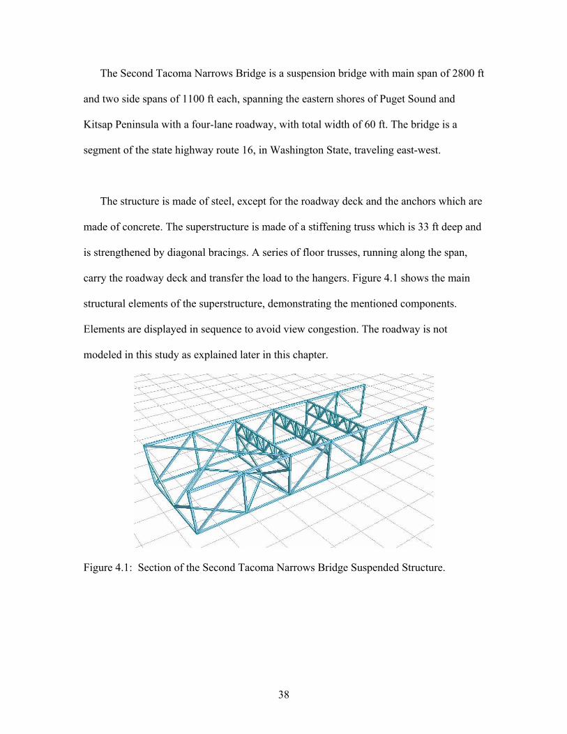
The Second Tacoma Narrows Bridge is a suspension bridge with main span of 2800 ft

and two side spans of 1100 ft each, spanning the eastern shores of Puget Sound and

Kitsap Peninsula with a four-lane roadway, with total width of 60 ft. The bridge is a

segment of the state highway route 16, in Washington State, traveling east-west.

The structure is made of steel, except for the roadway deck and the anchors which are

made of concrete. The superstructure is made of a stiffening truss which is 33 ft deep and

is strengthened by diagonal bracings. A series of floor trusses, running along the span,

carry the roadway deck and transfer the load to the hangers. Figure 4.1 shows the main

structural elements of the superstructure, demonstrating the mentioned components.

Elements are displayed in sequence to avoid view congestion. The roadway is not

modeled in this study as explained later in this chapter.

Figure 4.1: Section of the Second Tacoma Narrows Bridge Suspended Structure.

38

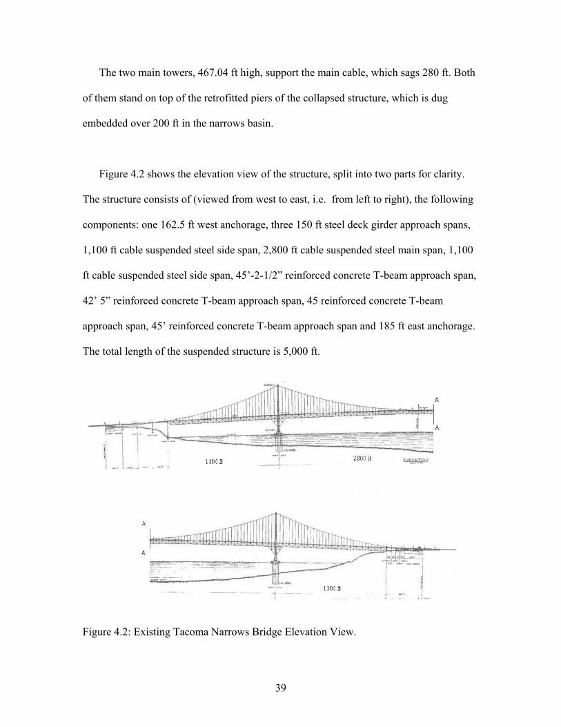
The two main towers, 467.04 ft high, support the main cable, which sags 280 ft. Both

of them stand on top of the retrofitted piers of the collapsed structure, which is dug

embedded over 200 ft in the narrows basin.

Figure 4.2 shows the elevation view of the structure, split into two parts for clarity.

The structure consists of (viewed from west to east, i.e. from left to right), the following

components: one 162.5 ft west anchorage, three 150 ft steel deck girder approach spans,

1,100 ft cable suspended steel side span, 2,800 ft cable suspended steel main span, 1,100

ft cable suspended steel side span, 45’-2-1/2” reinforced concrete T-beam approach span,

42’ 5” reinforced concrete T-beam approach span, 45 reinforced concrete T-beam

approach span, 45’ reinforced concrete T-beam approach span and 185 ft east anchorage.

The total length of the suspended structure is 5,000 ft.

Figure 4.2: Existing Tacoma Narrows Bridge Elevation View.

39

The deck width is 46’-8 1/8” which includes four 9 ft lanes separated by 2.75 ft

slotted wind grates and 1’-7” wind grates separating the roadway from the sidewalks. In

addition there are two 3.5 ft sidewalks, one on each side of roadway, and the width

between the suspension cables is 60 ft, as shown in Figure 4.5. The two main cables are

20.25 inches in diameter.

The tower’s total length is 467.04 ft, measured from the pier face. The tower’s legs

are made of steel segments, which are made of built-up sections of five rectangular

chambers arranged in cross-shape. The tower legs are tapered. The first 141.5 ft have a

parabolic tapering, 0.001x2 (ft), and the other segments are linearly tapered up to the top

of the tower. The legs are connected with lateral and diagonal bracings. Figure 4.4 shows

the elevation and the side views of the main tower.

The stiffening trusses are connected to the main tower legs at two points as shown in

the side view in Figure 4.4. A diamond-shaped truss element assembly embraces a giant

damper which is embedded inside each tower leg and connected to the upper cord of the

stiffening truss. Another assembly of truss elements connects the lower cord of the

stiffening truss to the face of the tower leg via a viscous damper. Both assemblies are

designed to dissipate any excessive excitation along the longitudinal direction of the

stiffening truss. The stiffening trusses are also connected to the middle part of the tower

via the horizontal upper chord bracings which connect the site of the upper cord to the

stiffening trusses. A “windshoe” is designed at the point where the upper chord bracings

are connected to the main tower lateral beam. The windshoe is simply a gap element

40

which allows movement along the bridge deck and around the tower axes. The other

displacements in the other degrees of freedoms are restrained.

The side spans have a linear slope of 3%. The main span is parabolic with 21 ft

difference in elevation between its ends at the towers and its mid span. It consists of 88

bays spaced at 30’ – 10 5/8” along the center span. The spacing of bays along the side

spans is 30’ – 3 3/8”.

4.4 Finite Element Model The choice of the finite element procedure is very important issue in the analysis of

suspension bridges. There are very few computer software packages that explicitly

support catenary cable element formulation. Procedures that do not support this feature

require special analysis procedure to obtain relatively close results.

The SAP 2000 was initially used for this purpose. However, the results from the

dynamic and the static analyses were inaccurate. It is found that SAP2000 does not

support explicit features to handle catenary cable elements and only supports non-linear

truss elements. Therefore prior to conducting frequency or dynamic analyses, it is

required to conduct a shape-finding analysis to determine the unstrained profile, followed

by a static stage construction analysis to build up the nonlinear geometric stiffness.

Furthermore, special constraints should be artificially added to the model to prevent local

instability.

41

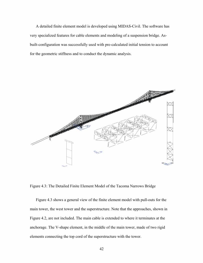
A detailed finite element model is developed using MIDAS-Civil. The software has

very specialized features for cable elements and modeling of a suspension bridge. As-

built-configuration was successfully used with pre-calculated initial tension to account

for the geometric stiffness and to conduct the dynamic analysis.

Figure 4.3: The Detailed Finite Element Model of the Tacoma Narrows Bridge

Figure 4.3 shows a general view of the finite element model with pull-outs for the

main tower, the west tower and the superstructure. Note that the approaches, shown in

Figure 4.2, are not included. The main cable is extended to where it terminates at the

anchorage. The V-shape element, in the middle of the main tower, made of two rigid

elements connecting the top cord of the superstructure with the tower.

42

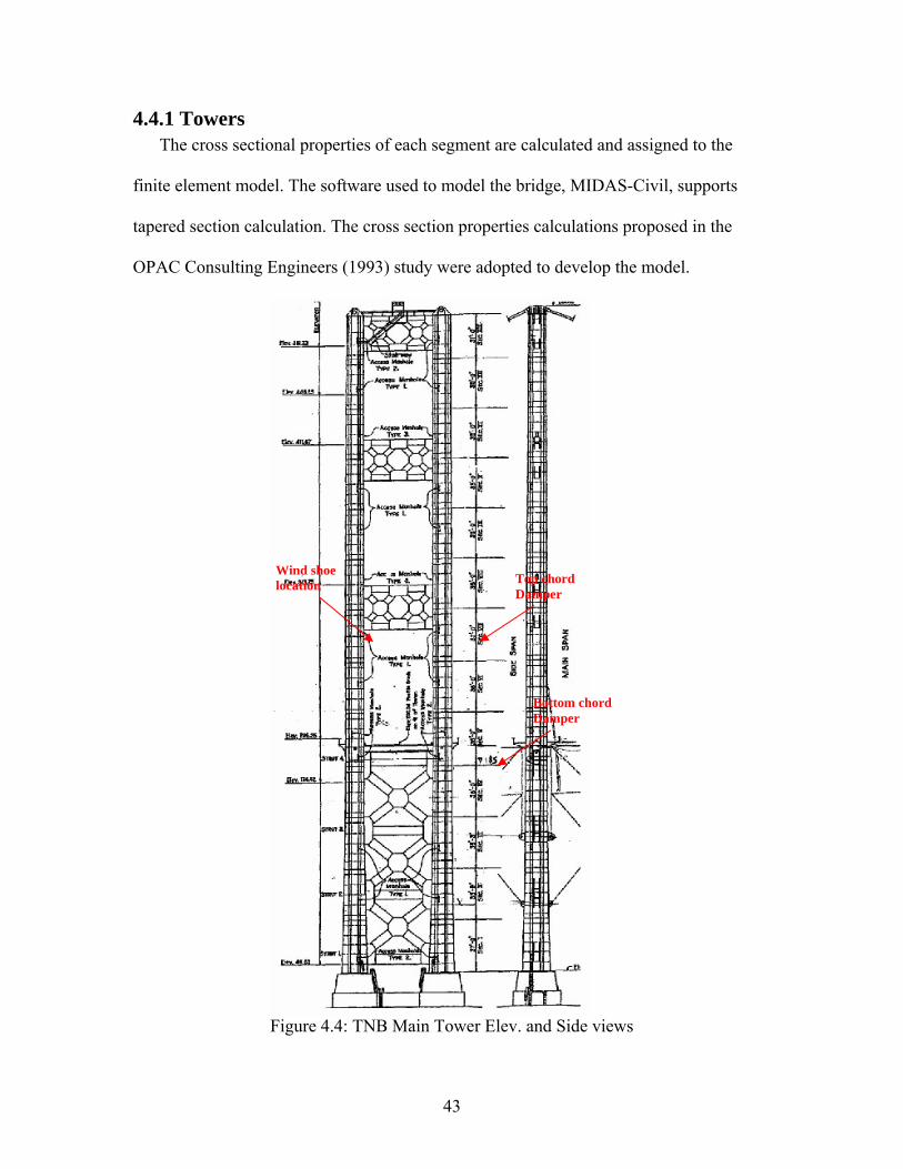
4.4.1 Towers The cross sectional properties of each segment are calculated and assigned to the

finite element model. The software used to model the bridge, MIDAS-Civil, supports

tapered section calculation. The cross section properties calculations proposed in the

OPAC Consulting Engineers (1993) study were adopted to develop the model.

F

W l Top chord

ind shoeocation

igure 4.4: TNB Main Tower Elev. and Side views

Damper

Bottom chord Damper

43

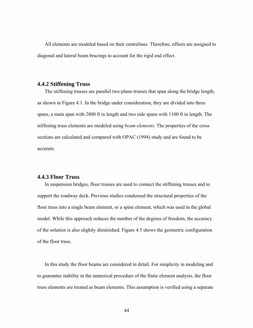
All elements are modeled based on their centrelines. Therefore, offsets are assigned to

diagonal and lateral beam bracings to account for the rigid end effect.

4.4.2 Stiffening Truss The stiffening trusses are parallel two-plane-trusses that span along the bridge length,

as shown in Figure 4.1. In the bridge under consideration, they are divided into three

spans, a main span with 2800 ft in length and two side spans with 1100 ft in length. The

stiffening truss elements are modeled using beam elements. The properties of the cross

sections are calculated and compared with OPAC (1994) study and are found to be

accurate.

4.4.3 Floor Truss In suspension bridges, floor trusses are used to connect the stiffening trusses and to

support the roadway deck. Previous studies condensed the structural properties of the

floor truss into a single beam element, or a spine element, which was used in the global

model. While this approach reduces the number of the degrees of freedom, the accuracy

of the solution is also slightly diminished. Figure 4.5 shows the geometric configuration

of the floor truss.

In this study the floor beams are considered in detail. For simplicity in modeling and

to guarantee stability in the numerical procedure of the finite element analysis, the floor

truss elements are treated as beam elements. This assumption is verified using a separate

44

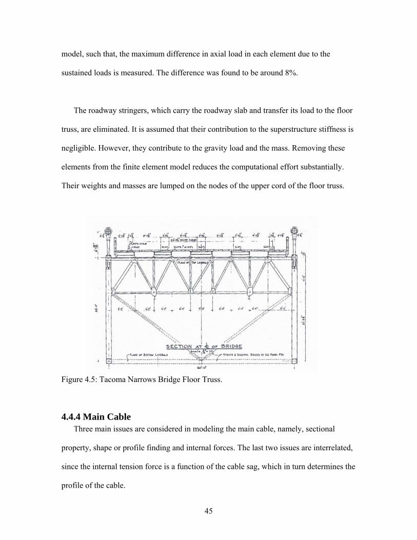
model, such that, the maximum difference in axial load in each element due to the

sustained loads is measured. The difference was found to be around 8%.

The roadway stringers, which carry the roadway slab and transfer its load to the floor

truss, are eliminated. It is assumed that their contribution to the superstructure stiffness is

negligible. However, they contribute to the gravity load and the mass. Removing these

elements from the finite element model reduces the computational effort substantially.

Their weights and masses are lumped on the nodes of the upper cord of the floor truss.

Figure 4.5: Tacoma Narrows Bridge Floor Truss.

4.4.4 Main Cable Three main issues are considered in modeling the main cable, namely, sectional

property, shape or profile finding and internal forces. The last two issues are interrelated,

since the internal tension force is a function of the cable sag, which in turn determines the

profile of the cable.

45

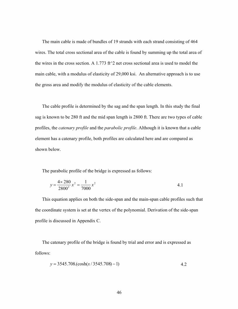
The main cable is made of bundles of 19 strands with each strand consisting of 464

wires. The total cross sectional area of the cable is found by summing up the total area of

the wires in the cross section. A 1.773 ft^2 net cross sectional area is used to model the

main cable, with a modulus of elasticity of 29,000 ksi. An alternative approach is to use

the gross area and modify the modulus of elasticity of the cable elements.

The cable profile is determined by the sag and the span length. In this study the final

sag is known to be 280 ft and the mid span length is 2800 ft. There are two types of cable

profiles, the catenary profile and the parabolic profile. Although it is known that a cable

element has a catenary profile, both profiles are calculated here and are compared as

shown below.

The parabolic profile of the bridge is expressed as follows:

222 7000

12800

2804 xxy =×

=

4.1

This equation applies on both the side-span and the main-span cable profiles such that

the coordinate system is set at the vertex of the polynomial. Derivation of the side-span

profile is discussed in Appendix C.

The catenary profile of the bridge is found by trial and error and is expressed as

follows:

)1)3545.708/.(cosh(3545.708 −= xy 4.2

46

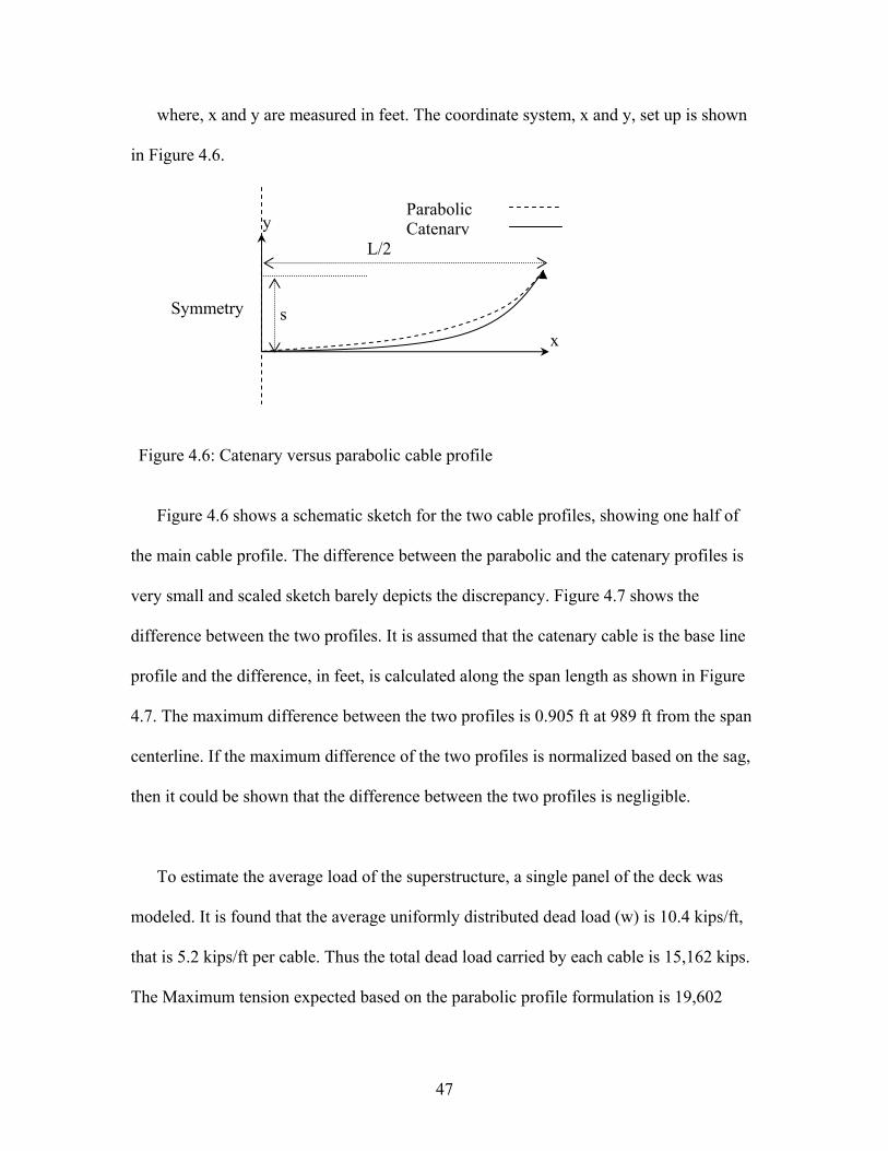
where, x and y are measured in feet. The coordinate system, x and y, set up is shown

in Figure 4.6.

Figure 4.6: Catenary versus parabolic cable profile

Figure 4.6 shows a schematic sketch for the two cable profiles, showing one half of

the main cable profile. The difference between the parabolic and the catenary profiles is

very small and scaled sketch barely depicts the discrepancy. Figure 4.7 shows the

difference between the two profiles. It is assumed that the catenary cable is the base line

profile and the difference, in feet, is calculated along the span length as shown in Figure

4.7. The maximum difference between the two profiles is 0.905 ft at 989 ft from the span

centerline. If the maximum difference of the two profiles is normalized based on the sag,

then it could be shown that the difference between the two profiles is negligible.

To estimate the average load of the superstructure, a single panel of the deck was

modeled. It is found that the average uniformly distributed dead load (w) is 10.4 kips/ft,

that is 5.2 kips/ft per cable. Thus the total dead load carried by each cable is 15,162 kips.

The Maximum tension expected based on the parabolic profile formulation is 19,602

Parabolic Catenary y

x

Symmetry

L/2

s

47

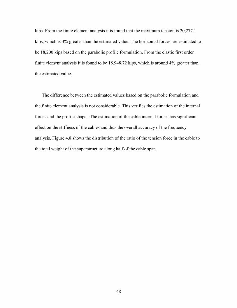
kips. From the finite element analysis it is found that the maximum tension is 20,277.1

kips, which is 3% greater than the estimated value. The horizontal forces are estimated to

be 18,200 kips based on the parabolic profile formulation. From the elastic first order

finite element analysis it is found to be 18,948.72 kips, which is around 4% greater than

the estimated value.

The difference between the estimated values based on the parabolic formulation and

the finite element analysis is not considerable. This verifies the estimation of the internal

forces and the profile shape. The estimation of the cable internal forces has significant

effect on the stiffness of the cables and thus the overall accuracy of the frequency

analysis. Figure 4.8 shows the distribution of the ratio of the tension force in the cable to

the total weight of the superstructure along half of the cable span.

48

0

0.2

0.4

0.6

0.8

1

0 200 400 600 800 1000 1200 1400

Main Span (ft)

Diff

eren

ce B

etw

een

Pro

files

(ft)

Figure 4.7: Difference between catenary profile and parabolic profile along the main span length

Normalized Tension

1.24

1.26

1.28

1.3

1.32

1.34

1.36

0 200 400 600 800 1000 1200 1400

Distance ft

Forc

e / T

otal

Stru

ctur

al W

eigh

t

Normalized Tension

Figure 4.8: Normalized tension in main cable

While in suspension bridges, gravity loads are transferred to the main cable via

discrete hangers and hence applied as concentrated load, it is assumed here that the load

carried by the hanger is a uniformly distributed gravity load in order to determine the

shape of the cable.

49

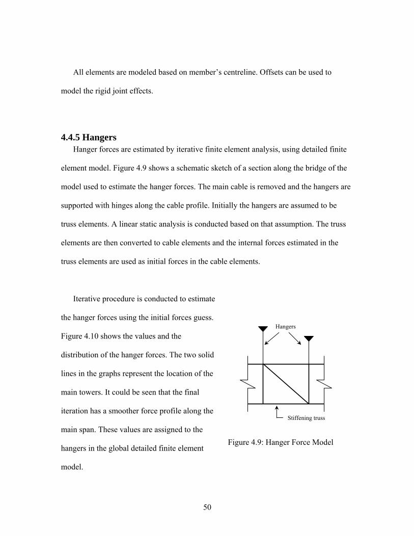
All elements are modeled based on member’s centreline. Offsets can be used to

model the rigid joint effects.

4.4.5 Hangers Hanger forces are estimated by iterative finite element analysis, using detailed finite

element model. Figure 4.9 shows a schematic sketch of a section along the bridge of the

model used to estimate the hanger forces. The main cable is removed and the hangers are

supported with hinges along the cable profile. Initially the hangers are assumed to be

truss elements. A linear static analysis is conducted based on that assumption. The truss

elements are then converted to cable elements and the internal forces estimated in the

truss elements are used as initial forces in the cable elements.

Iterative procedure is conducted to estimate

the hanger forces using the initial forces guess.

Figure 4.10 shows the values and the

distribution of the hanger forces. The two solid

lines in the graphs represent the location of the

main towers. It could be seen that the final

iteration has a smoother force profile along the

main span. These values are assigned to the

hangers in the global detailed finite element

model.

Hangers

Figure 4.9: Hanger Force Model

Stiffening truss

50

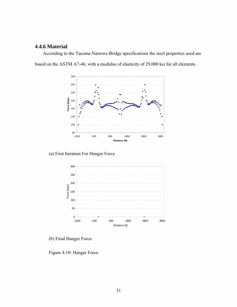
4.4.6 Material According to the Tacoma Narrows Bridge specifications the steel properties used are

based on the ASTM A7-46, with a modulus of elasticity of 29,000 ksi for all elements.

90

100

110

120

130

140

150

160

-1200 -200 800 1800 2800 3800

Distance (ft)

Forc

e (k

ips)

(a) First Iteration For Hanger Force

0

50

100

150

200

250

300

-1200 -200 800 1800 2800 3800

Distance (ft)

Forc

e (k

ips)

(b) Final Hanger Force

Figure 4.10: Hanger Force

51

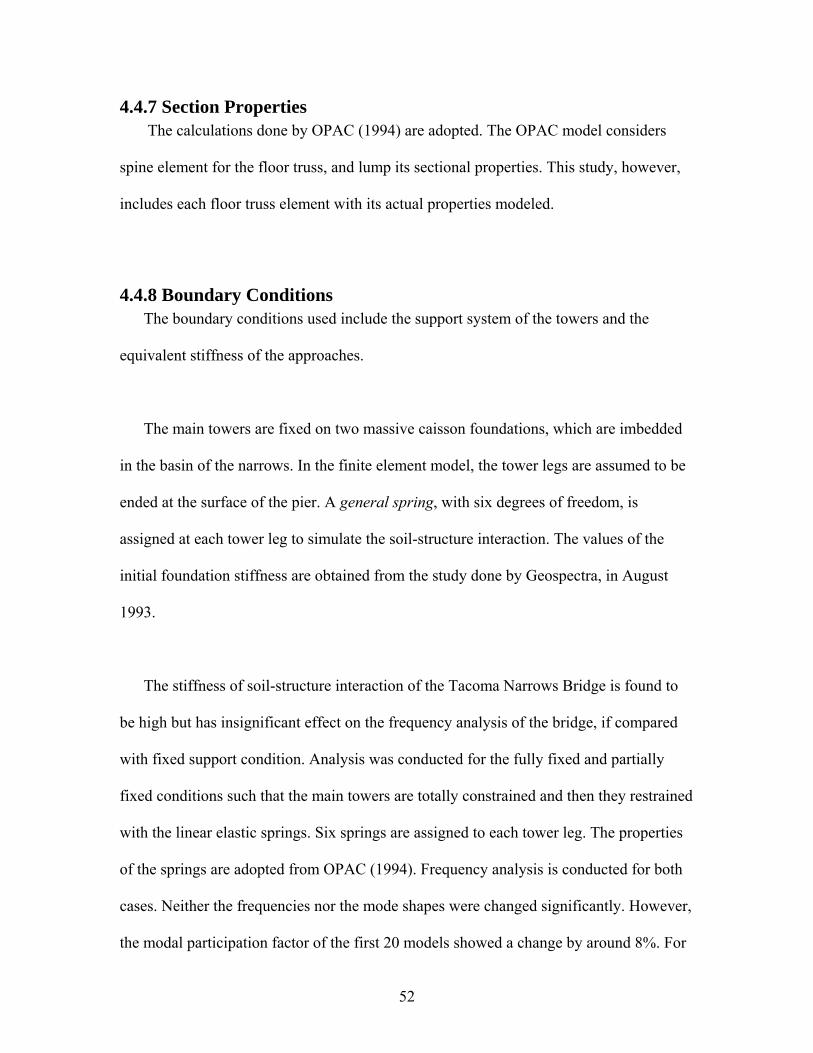
4.4.7 Section Properties The calculations done by OPAC (1994) are adopted. The OPAC model considers

spine element for the floor truss, and lump its sectional properties. This study, however,

includes each floor truss element with its actual properties modeled.

4.4.8 Boundary Conditions The boundary conditions used include the support system of the towers and the

equivalent stiffness of the approaches.

The main towers are fixed on two massive caisson foundations, which are imbedded

in the basin of the narrows. In the finite element model, the tower legs are assumed to be

ended at the surface of the pier. A general spring, with six degrees of freedom, is

assigned at each tower leg to simulate the soil-structure interaction. The values of the

initial foundation stiffness are obtained from the study done by Geospectra, in August

1993.

The stiffness of soil-structure interaction of the Tacoma Narrows Bridge is found to

be high but has insignificant effect on the frequency analysis of the bridge, if compared

with fixed support condition. Analysis was conducted for the fully fixed and partially

fixed conditions such that the main towers are totally constrained and then they restrained

with the linear elastic springs. Six springs are assigned to each tower leg. The properties

of the springs are adopted from OPAC (1994). Frequency analysis is conducted for both

cases. Neither the frequencies nor the mode shapes were changed significantly. However,

the modal participation factor of the first 20 models showed a change by around 8%. For

52

more accuracy analysis, the equivalent linear springs of the initial foundation stiffness

were used.

The effect of removing the approaches is modeled as linear elastic springs. The

equivalent stiffness of the west approach is added as three linear springs distributed on

the top beam of tower number 3. The approach is modeled separately, such that static

forces are applied to determine the equivalent stiffness values which were estimated at

226570 kips/ft and 73.2 kips/ft for the longitudinal and the transverse directions,

respectively. The east tower is very short in length and made of concrete. The east

approach is assumed sufficiently rigid and it is modeled as hinge support. The east

approach is also excluded from the model. This will not have a significant effect on wind

analysis, and will not influence the frequency content.

The two anchors, supporting the main cables and transferring their internal forces to

the ground are modeled as hinges, at their corresponding locations. The anchors may

experience slight movement in case of earthquakes, but their displacements are negligible

if wind loading is considered.

4.4.9 Nonlinear elements According to a field investigation, the tower top chord damper installed inside the

tower were found to be leaking. These dampers are never replaced because of

impracticality. It is difficult to estimate their response based on the provided

53

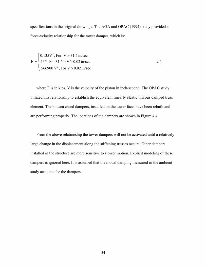
specifications in the original drawings. The AGA and OPAC (1994) study provided a

force-velocity relationship for the tower damper, which is:

⎪⎩

⎪⎨

⎧

>

≥≥>

=

in/sec 0.02 VFor ,V 566900 in/sec 0.02 V 31.5For , 135

in/sec 31.5VFor ,0.135V F

2

2

4.3

where F is in kips, V is the velocity of the piston in inch/second. The OPAC study

utilized this relationship to establish the equivalent linearly elastic viscous damped truss

element. The bottom chord dampers, installed on the tower face, have been rebuilt and

are performing properly. The locations of the dampers are shown in Figure 4.4.

From the above relationship the tower dampers will not be activated until a relatively

large change in the displacement along the stiffening trusses occurs. Other dampers

installed in the structure are more sensitive to slower motion. Explicit modeling of these

dampers is ignored here. It is assumed that the modal damping measured in the ambient

study accounts for the dampers.

54

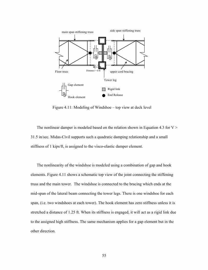
side span stiffening truss main span stiffening truss

Figure 4.11: Modeling of Windshoe – top view at deck level

The nonlinear damper is modeled based on the relation shown in Equation 4.3 for V >

31.5 in/sec. Midas-Civil supports such a quadratic damping relationship and a small

stiffness of 1 kips/ft, is assigned to the visco-elastic damper element.

The nonlinearity of the windshoe is modeled using a combination of gap and hook

elements. Figure 4.11 shows a schematic top view of the joint connecting the stiffening

truss and the main tower. The windshoe is connected to the bracing which ends at the

mid-span of the lateral beam connecting the tower legs. There is one windshoe for each

span, (i.e. two windshoes at each tower). The hook element has zero stiffness unless it is

stretched a distance of 1.25 ft. When its stiffness is engaged, it will act as a rigid link due

to the assigned high stiffness. The same mechanism applies for a gap element but in the

other direction.

Tower leg

Distance = 0 ft upper cord bracing

Hook element

Gap element Rigid link

Floor truss

End Release

55

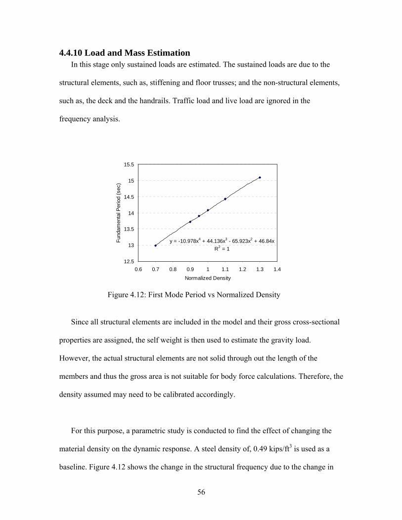
4.4.10 Load and Mass Estimation In this stage only sustained loads are estimated. The sustained loads are due to the

structural elements, such as, stiffening and floor trusses; and the non-structural elements,

such as, the deck and the handrails. Traffic load and live load are ignored in the

frequency analysis.

y = -10.978x4 + 44.136x3 - 65.923x2 + 46.84xR2 = 1

12.5

13

13.5

14

14.5

15

15.5

0.6 0.7 0.8 0.9 1 1.1 1.2 1.3 1.4Normalized Density

Fund

amen

tal P

erio

d (s

ec)

Figure 4.12: First Mode Period vs Normalized Density

Since all structural elements are included in the model and their gross cross-sectional

properties are assigned, the self weight is then used to estimate the gravity load.

However, the actual structural elements are not solid through out the length of the

members and thus the gross area is not suitable for body force calculations. Therefore, the

density assumed may need to be calibrated accordingly.

For this purpose, a parametric study is conducted to find the effect of changing the

material density on the dynamic response. A steel density of, 0.49 kips/ft3 is used as a

baseline. Figure 4.12 shows the change in the structural frequency due to the change in

56

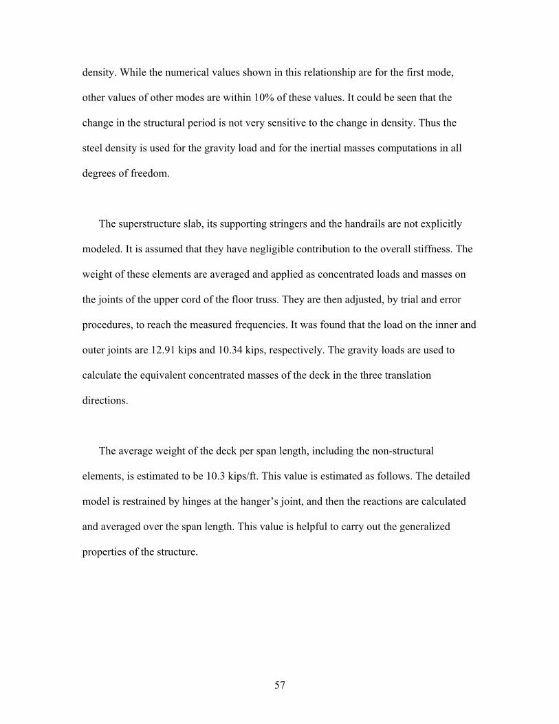
density. While the numerical values shown in this relationship are for the first mode,

other values of other modes are within 10% of these values. It could be seen that the

change in the structural period is not very sensitive to the change in density. Thus the

steel density is used for the gravity load and for the inertial masses computations in all

degrees of freedom.

The superstructure slab, its supporting stringers and the handrails are not explicitly

modeled. It is assumed that they have negligible contribution to the overall stiffness. The

weight of these elements are averaged and applied as concentrated loads and masses on

the joints of the upper cord of the floor truss. They are then adjusted, by trial and error

procedures, to reach the measured frequencies. It was found that the load on the inner and

outer joints are 12.91 kips and 10.34 kips, respectively. The gravity loads are used to

calculate the equivalent concentrated masses of the deck in the three translation

directions.

The average weight of the deck per span length, including the non-structural

elements, is estimated to be 10.3 kips/ft. This value is estimated as follows. The detailed

model is restrained by hinges at the hanger’s joint, and then the reactions are calculated

and averaged over the span length. This value is helpful to carry out the generalized

properties of the structure.

57

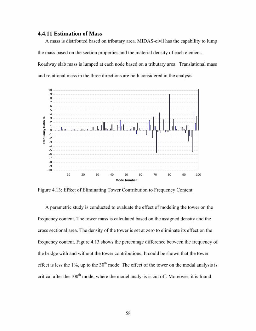
4.4.11 Estimation of Mass A mass is distributed based on tributary area. MIDAS-civil has the capability to lump

the mass based on the section properties and the material density of each element.

Roadway slab mass is lumped at each node based on a tributary area. Translational mass

and rotational mass in the three directions are both considered in the analysis.

-10-9-8-7-6-5-4-3-2-10123456789

10

10 20 30 40 50 60 70 80 90 100

Mode Number

Freq

uanc

y Ra

tio %

Figure 4.13: Effect of Eliminating Tower Contribution to Frequency Content

A parametric study is conducted to evaluate the effect of modeling the tower on the

frequency content. The tower mass is calculated based on the assigned density and the

cross sectional area. The density of the tower is set at zero to eliminate its effect on the

frequency content. Figure 4.13 shows the percentage difference between the frequency of

the bridge with and without the tower contributions. It could be shown that the tower

effect is less the 1%, up to the 30th mode. The effect of the tower on the modal analysis is

critical after the 100th mode, where the model analysis is cut off. Moreover, it is found

58

from the modal analysis that the frequencies related to the superstructure oscillation are

found between the first and the fiftieth modes.

The parametric study verifies that uncertainty in the tower modeling is not of concern

for wind analysis of the bridge superstructure. It is evident that the frequencies governing

the tower vibration are beyond those of the superstructure.

The finite element model is used to estimate the uniformly distributed weight over the

span length of the deck such that the reactions of the hangers are summed and distributed

over the span length. The uniformly distributed load over the span length is estimated to

be around 8433.7 lb/ft (255.8 slug/ft), which is equivalent to a uniformly distributed mass

of 12,451.5 kg/m.

4.5 Frequency Analysis

4.5.1 Ambient Study Ambient vibration measurements were taken by the Johns Hopkins University under

the supervision of Dr. Nicholas Jones in 1993. The mode shapes and the damping ratios

of the bridge are derived from the data generated. The ambient study comprised both

transient vibration and ambient vibration measurements. The transient measurements are

the vibrations recorded after a sudden release of energy, such as impacting the structure

with a large load. This approach is used to estimate the frequency of the superstructure.

Ambient measurements are the vibrations produced by traffic and wind. This approach is

useful to estimate both the deck and the towers frequencies. For best transient

59

measurement analysis, the records should be taken when the ambient vibrations are

minimal.

The transient measurements captured the first mode of vibration, 0.074 Hz. The

second mode was not captured. The third mode, predominantly vertical mode; the fourth

mode, center-span lateral mode; the fifth mode, center-span vertical and the sixth mode,

center-span lateral mode, are also captured by the transient analysis. The ambient

measurements revealed the first 9 vertical, 1 torsional and 12 lateral natural frequencies.

The damping ratio was determined to be in the range of 0.3% to 3.5% and the study

concluded that the average damping is 1.3%, which is a reasonable number and close to

the true value for the size of the Tacoma Narrows Bridge when operating within the

elastic range. The results of the natural frequency are shown with the frequency analysis

results are presented below. The average damping ratio of the bridge is relatively small in

magnitude. Therefore its influence on the damped natural frequency is insignificant and

could be considered equal to the undamped natural frequency.

4.5.2 Eigenvalue Analysis In the analysis, 100 Ritz vectors are generated, that is, one hundred modes and

frequencies are estimated. The mode shapes and frequencies obtained from the analysis

are found to compare reasonably well with experimental studies as shown in Table 4.1.

60

4.5.3 Model Calibration and Analysis The following procedure was used to calibrate the model:

1. Pre-modelling Phase:

a. Evaluation of the bridge detailed drawings.

b. Review previous studies on the bridge.

c. Develop a 3-D CAD model for the bridge geometry.

2. Structural Modelling Phase:

d. Transfer the CAD model to the structural analysis program (MIDAS-

Civil).

e. Calculate gross cross sectional properties.

f. Compute the weights of non-structural elements.

g. Estimate boundary condition of foundations and the approaches.

h. Approximate the initial tension in the main cable and hangers, using the

elastic theory.

i. Iterate the cable forces.

j. Solve Eigen value problem, using the Ritz theory method.

3. Model Calibration

k. Calibrate the estimated sustained loads and re-evaluate the cable initial

tension.

l. Calibrate boundary condition.

m. Calibrate selfweight, by tuning the material density.

n. Evaluate the modal response and reiterate, as needed.

61

4.6 Results Table 4.1 lists the bridge frequencies. Experimental frequencies are obtained from the

ambient vibration taken by the Johns Hopkins University in September, 1993. The

analytical results are estimated using MIDAS-civil. Ritz vector is used in the Eigenvalue

analysis. The table shows the results of the OPAC (1994) study. The error percentage

shown is the analytical results, obtained in this research, to the corresponding

experimental frequency.

Table 4.2 shows thirteen modes of vibration for the Tacoma Narrows Bridge. The

identified modes are only those vertical, transverse and torsional modes of vibration.

Appendix A shows complete identification of the bridge mode shapes and their locations.

Periods after the 50th mode are found to be relatively very small, less than 1.5 second, for

wind analysis.

62

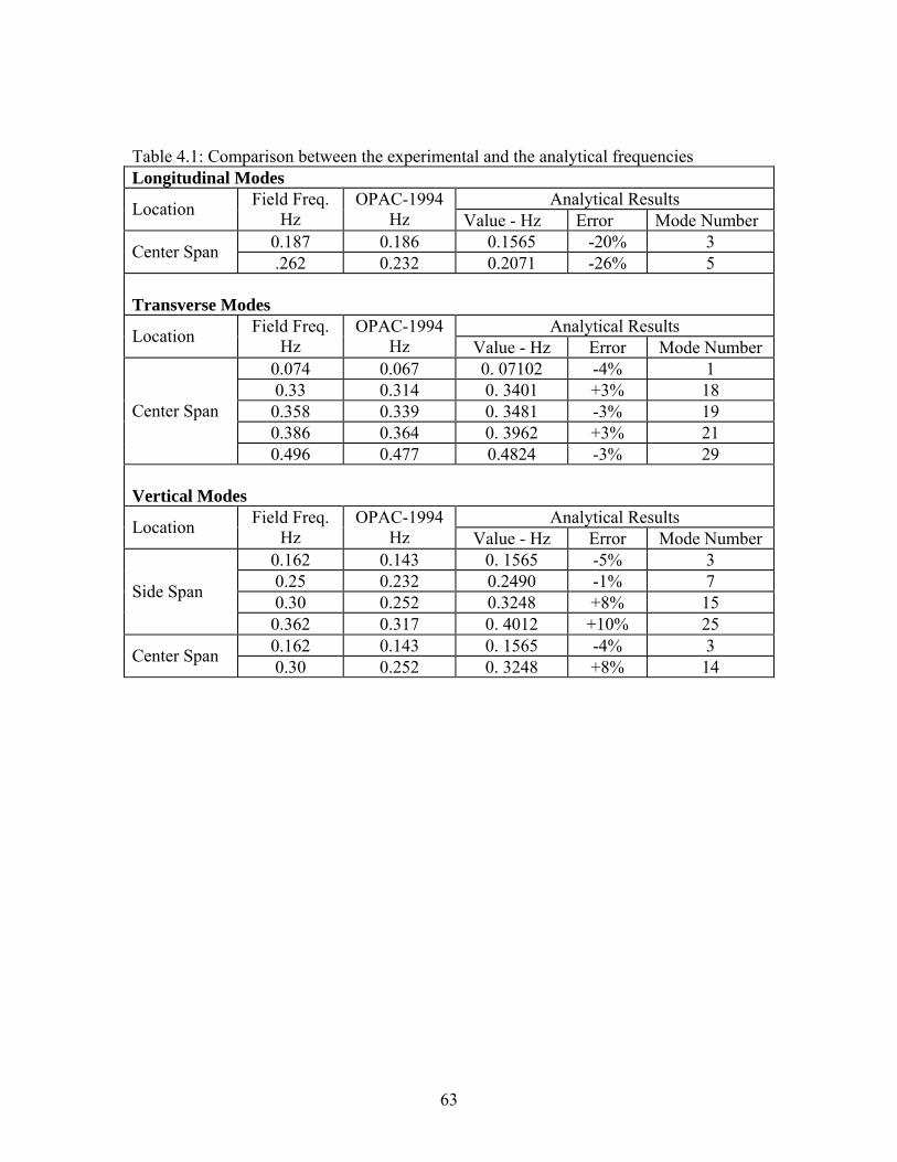
Table 4.1: Comparison between the experimental and the analytical frequencies Longitudinal Modes

Analytical Results Location Field Freq. Hz

OPAC-1994 Hz Value - Hz Error Mode Number

0.187 0.186 0.1565 -20% 3 Center Span .262 0.232 0.2071 -26% 5 Transverse Modes

Analytical Results Location Field Freq. Hz

OPAC-1994 Hz Value - Hz Error Mode Number

0.074 0.067 0. 07102 -4% 1 0.33 0.314 0. 3401 +3% 18 0.358 0.339 0. 3481 -3% 19 0.386 0.364 0. 3962 +3% 21

Center Span

0.496 0.477 0.4824 -3% 29 Vertical Modes

Analytical Results Location Field Freq. Hz

OPAC-1994 Hz Value - Hz Error Mode Number

0.162 0.143 0. 1565 -5% 3 0.25 0.232 0.2490 -1% 7 0.30 0.252 0.3248 +8% 15 Side Span

0.362 0.317 0. 4012 +10% 25 0.162 0.143 0. 1565 -4% 3 Center Span 0.30 0.252 0. 3248 +8% 14

63

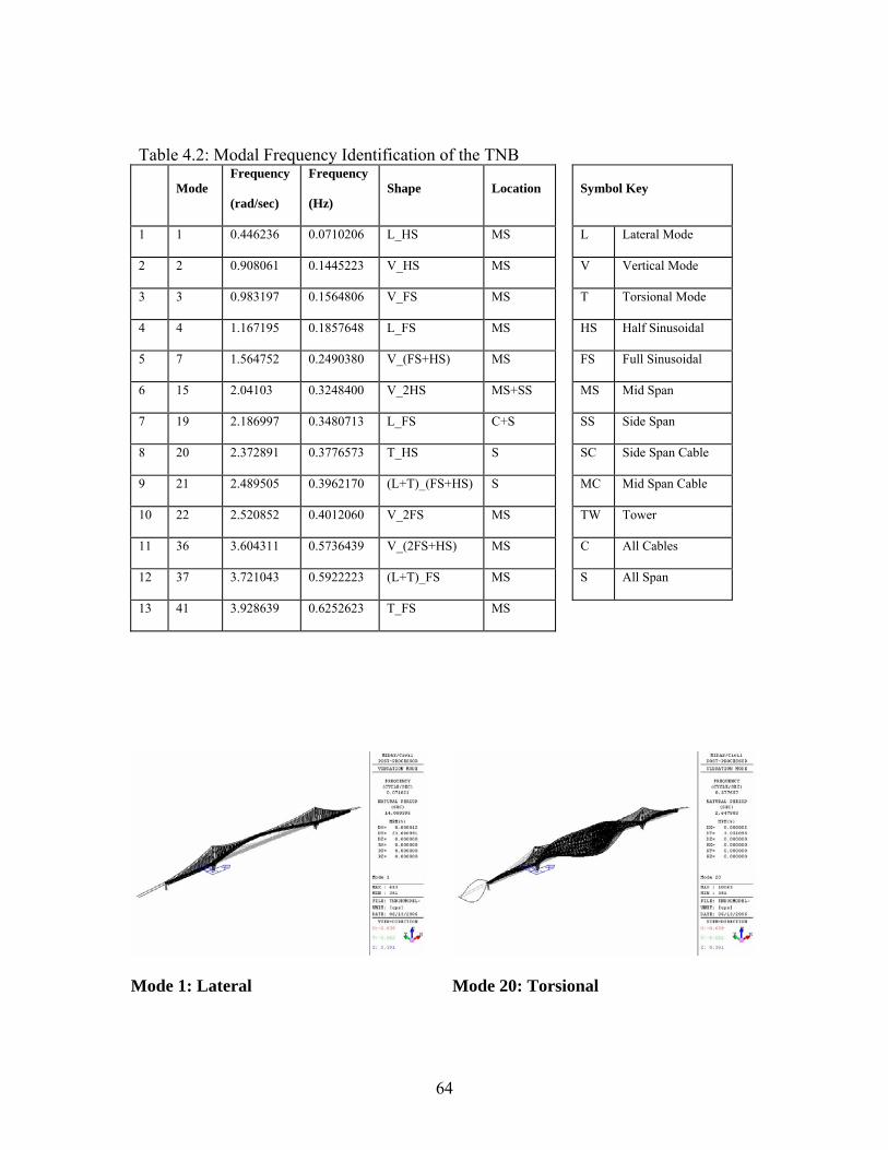
Table 4.2: Modal Frequency Identification of the TNB

Mode Frequency

(rad/sec)

Frequency

(Hz) Shape Location Symbol Key

1 1 0.446236 0.0710206 L_HS MS L Lateral Mode

2 2 0.908061 0.1445223 V_HS MS V Vertical Mode

3 3 0.983197 0.1564806 V_FS MS T Torsional Mode

4 4 1.167195 0.1857648 L_FS MS HS Half Sinusoidal

5 7 1.564752 0.2490380 V_(FS+HS) MS FS Full Sinusoidal

6 15 2.04103 0.3248400 V_2HS MS+SS MS Mid Span

7 19 2.186997 0.3480713 L_FS C+S SS Side Span

8 20 2.372891 0.3776573 T_HS S SC Side Span Cable

9 21 2.489505 0.3962170 (L+T)_(FS+HS) S MC Mid Span Cable

10 22 2.520852 0.4012060 V_2FS MS TW Tower

11 36 3.604311 0.5736439 V_(2FS+HS) MS C All Cables

12 37 3.721043 0.5922223 (L+T)_FS MS S All Span

13 41 3.928639 0.6252623 T_FS MS

Mode 1: Lateral

Mode 20: Torsional

64

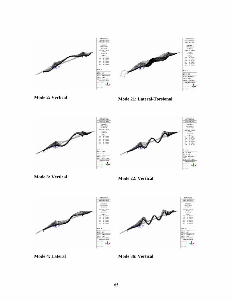
Mode 2: Vertical

Mode 21: Lateral-Torsional

Mode 3: Vertical

Mode 22: Vertical

Mode 4: Lateral

Mode 36: Vertical

65

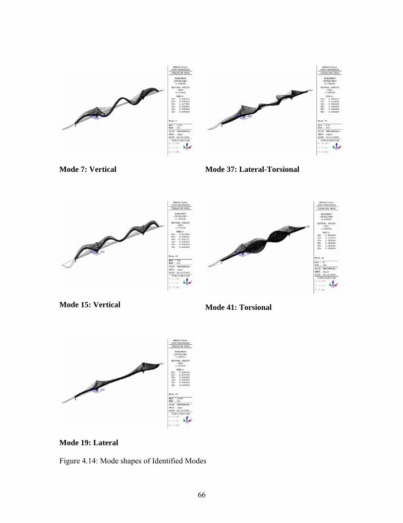
Mode 7: Vertical

Mode 37: Lateral-Torsional

Mode 15: Vertical

Mode 41: Torsional

Mode 19: Lateral

Figure 4.14: Mode shapes of Identified Modes

66

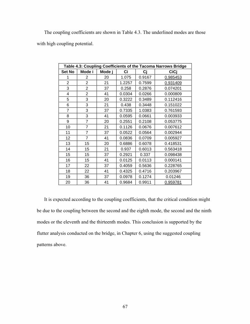
The coupling coefficients are shown in Table 4.3. The underlined modes are those

with high coupling potential.

Table 4.3: Coupling Coefficients of the Tacoma Narrows Bridge Set No Mode i Mode j Ci Cj CiCj

1 2 20 1.075 0.9167 0.985453 2 2 21 1.2257 0.7599 0.931409 3 2 37 0.258 0.2876 0.074201 4 2 41 0.0304 0.0266 0.000809 5 3 20 0.3222 0.3489 0.112416 6 3 21 0.438 0.3448 0.151022 7 3 37 0.7335 1.0383 0.761593 8 3 41 0.0595 0.0661 0.003933 9 7 20 0.2551 0.2108 0.053775 10 7 21 0.1126 0.0676 0.007612 11 7 37 0.0522 0.0564 0.002944 12 7 41 0.0836 0.0709 0.005927 13 15 20 0.6886 0.6078 0.418531 14 15 21 0.937 0.6013 0.563418 15 15 37 0.2921 0.337 0.098438 16 15 41 0.0125 0.0113 0.000141 17 22 37 0.4059 0.5636 0.228765 18 22 41 0.4325 0.4716 0.203967 19 36 37 0.0978 0.1274 0.01246 20 36 41 0.9684 0.9911 0.959781

It is expected according to the coupling coefficients, that the critical condition might

be due to the coupling between the second and the eighth mode, the second and the ninth

modes or the eleventh and the thirteenth modes. This conclusion is supported by the

flutter analysis conducted on the bridge, in Chapter 6, using the suggested coupling

patterns above.

67

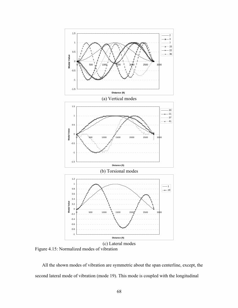
-1.5

-1

-0.5

0

0.5

1

1.5

0 500 1000 1500 2000 2500 3000

Distance (ft)

Mod

al V

alue

237152236

(a) Vertical modes

-1.5

-1

-0.5

0

0.5

1

1.5

0 500 1000 1500 2000 2500 3000

Distance (ft)

Mod

al V

alue

20213741

(b) Torsional modes

-1

-0.8

-0.6

-0.4

-0.2

0

0.2

0.4

0.6

0.8

1

1.2

0 500 1000 1500 2000 2500 3000

Distance (ft)

Mod

al V

alue

119

(c) Lateral modes

Figure 4.15: Normalized modes of vibration

All the shown modes of vibration are symmetric about the span centerline, except, the

second lateral mode of vibration (mode 19). This mode is coupled with the longitudinal

68

mode which transports the effect of the asymmetric boundary condition to the lateral

mode. It could be noted that the curve amplitude attenuates from left to right and the

curve matches with the point of symmetry at the centreline of the mid-span. This is due to

the effect of the eastern boundary condition (at the right-hand-side side-span), which is

stiffer than the boundary condition at the other end of the western side-span.

4.7 Discussion Table 4.1 shows the frequencies obtained from the ambient analysis, OPAC (1994)

study and this research. Note that the frequencies evaluated using the proposed

methodology are relatively accurate when compared with the experimental results. The

error in the transverse and the vertical modes is not more than 10%. This error is very

acceptable. However, the frequencies of the longitudinal direction are less accurate.

Unlike the superstructure transverse and the vertical modes of vibration, the

longitudinal mode of vibration of the deck interacts with the tower and the approaches

boundary conditions. In other words, the modeling of these two components reflects on

the accuracy of the superstructure frequencies in that direction. A 26% error in the

frequency is not faulty results for the following reasons. The tower and the approaches,

most likely, will not interact with the deck movement, because the windshoe and the

expansion joints provide enough separation. Moreover, the longitudinal mode shapes are

not significant in wind. The deck is assumed to be sufficiently rigid along its axis and

only excitations in the transverse, vertical and rotational are considered. The frequencies

in this direction shall be further calibrated if seismic analysis is required.

69

The results obtained here are more accurate than those of the OPAC (1994) study.

Note that most of the section properties, boundary conditions and mass estimations used

in this research are based on the OPAC study. The study, however, used linear cable

element instead of catenary cable element. This proves that using catenary cable element

with appropriate initial tension estimation is essential for accurate frequency analysis.

There are several factors that affect the frequencies of the structure. The most

important factors include mass estimation and distribution, element stiffness and initial

tension in the cables. Boundary conditions and soil structure interaction are of less

significance. The towers have small influence on the low structural frequencies, and their

effects are significant only after the 50th mode. Thus, the superstructure and cable

properties have the most impact in the lower frequency range.

70

CHAPTER 5 BRIDGE AEROELASTICITY 5.1 Background

The failure of the Original Tacoma Narrows Bridge was a pivot point in the history of

suspension bridges, as it coincided with the evolution of aeronautical engineering. Thus

the failure was justified, unlike prior bridge catastrophes. Vortex-induced and flutter

forces become well-recognized as the main phenomena responsible for long-span bridge

collapse.

Classical aerodynamic theories of wind forces are based on steady-state expressions

such as Bernoulli’s equation, and solved using the quasi-static approach. However, this

type of formulation is insufficient to describe the rapid time-varying forces that develop

at higher speeds. Moreover, steady-state functions will not allow expressing the self-

induced forces, resulting from the change in deformations or deflections due to time.

Therefore, it was necessary to develop more general theories to account for time

variation. Theories that followed the quasi-static approach were based on transient

dynamic analysis. Earlier tests started on airfoil in laminar wind flow followed by studies

of bluff bodies.

5.2 Earlier Aeroelasticity Theories The first insightful view into self-induced forces was investigated by Wagner (1925),

using thin aerofoil with various angles of attack. He proposed a very illustrative indicial

function to express lift force for thin airfoil undergoing a step change in the angle of

71

attack in incompressible flow. Theodorsen (1934) presented his function which was later

considered as a fundamental function in unsteady aerodynamics on oscillating thin airfoil

in incompressible flow. The function is described in complex terms with respect to time-

frequency domain. The function is considered as a reference in developing flutter

formulation for a bluff body, as described by Scanlan and Tomko (1971). Kussner (1936)

then presented the theoretical bases of flutter forces and guest penetration for a thin

airfoil . Garrick (1938) investigated the foregoing theories and found the relations among

them using Fourier transformation. He thus proved the interrelation among all of these

theories of non-stationary flows. Sears (1941) proposed an admittance function named

after him which is now a well-known function in the frequency domain analysis. In 1941,

Von Karman and Sears investigated flutter of a thin airfoil moving into a sinusoidal

vertical velocity (gust) filed. Sears problem shows the fundamental difference between

the results obtained on an oscillating airfoil in angle of attack and an airfoil moving

through an oscillating vertical velocity field, where the latter results in a non-uniform

angle of attack over the airfoil chord. The Sear’s function is formulated in the frequency

domain, similar to the Theodorsen function (1934).

The Theodersen Function is applicable in many cases of both fixed-wing and

rotating-wing aerodynamics. However, they are less capable in other problems where

time is an important parameter where the velocity of the elastic body is not usually

constant. Thus, the reduced frequency term (K=UB/ω) becomes very ambiguous in this

case, where U is the oncoming wind velocity, B is the characteristic geometric parameter

(usually the width of the elastic body) and ω is the circular frequency of motion. Theories

72

formulated in time-domain are more general as they account for the varying or arbitrary

velocity of the solid body in the flow. However, as mentioned before, Wagner (1925)

obtained a solution for the indicial lift on a thin-airfoil undergoing a step change in the

angle of attack in incompressible flow. He introduced terms that represent the flow taking

into account the effect of time-history change of the angle of attack on the lift.

Sisto published a paper on stall flutter of airfoil while Liepmann (1952) applied the

forgoing theories in conjunction with statistical concepts to outline the random buffeting

problem of aircraft lifting surfaces, considering the Sears admittance function in that

process.

5.3 Early Bridge Aeroelasticity Theories After the collapse of the Tacoma Narrows bridge in 1940, a board of engineers

consisting of O.H. Ammann, T. Von Karman and G.B. Woodruff issued a detailed report

concerning the catastrophic failure . The report included a paper by Louis G. Dunn

explaining the phenomenon of vortex-shedding with the equation of motion, and giving a

detailed account of some of the earliest deck sections that collapsed, in particular those

that have negative aerodynamic damping and torsional flutter.

The explanation by Dunn was followed by an analysis of bridge flutter. Bleich (1948)

and Bleich (1949) used the Theodersen theory for flat plate for the analysis of bridge

flutter. The results, however, were not applicable to unstreamlined bridge decks. The

reason is that the Theodersen function was derived for thin flat plates. An alternative

73

approach, originally recommended by Dunn in the Tacoma Narrows Bridge case,

emerged suggesting that if motional force coefficients (flutter derivatives) are obtained

experimentally, they might be useful in the analysis. This idea was widely adopted and

used in the investigation. It became the fundamental idea in the theory of bridge

aeroelasticity. Davenport (1962) adopted steady-flow formulation flowing Liepmann’s

approach and the Sears admittance function to analyze bridge buffeting.

The theory of bridge aeroelasticity was established late in the 60’s with most of the

effort undertaken in the US and Japan. In the US, most of the research was attributed to

Scanlan, who outlined the flutter theory based on measured motional aerodynamic

derivatives. Scanlan’s contribution in aeroelasticity started in 1951 by investigating

aircraft vibration and flutter. In 1967, Scanlan and Sabzevari presented a conference

paper revisiting the analysis of bridge flutter based on experimental flutter derivatives.

Meanwhile, Ukeguchi, Sakata and Nishitani released a study on bridge flutter based on

the experimentally measured flutter derivatives theory, proposed by Scanlan and

Rosenbaum. Another contribution was made by Tanaka and Ito (1969) on the

characteristics of the aerodynamic forces of self-excited oscillations of bluff structures.

The concept proposed by Bleich (1948) to use the flat plate theory in bridge

aeroelasticity was revisited in 1971. Flutter derivatives of streamlined bodies were

experimentally investigated and compared to the theoretical flutter derivatives of airfoils,

so that the former will be applied to bridges. Sakata (1971) found that the thin airfoil

flutter theory was reasonable to apply on streamlined bridge deck sections. He

74

recommended his findings to the design of the Severn Bridge, which was the first ever to

be constructed with thin streamlined deck. However, Scanlan and Tomko (1971) tested

sets of flutter derivatives for bridges and compared them to the airfoil derivatives. They

concluded that bridge flutter derivatives are significantly different from airfoil

derivatives. Accordingly flutter derivatives of bridges are not accurately expressed by

analytical or mathematical solutions and experimental data is needed to characterize

them.

Another research approach was pursued to solve the equation of motion in

conjunction with the self-excited forces. The need to link the frequency domain with the

time domain was realized by Scanlan and Budlong (1972), where the Fourier

transformation was used to link the bridge deck flutter derivative and the distinct

aerodynamic force functions that were functions of both time and frequency. Thus the

right-hand-side of the equation of motion of self-induced forces became a function of the

frequency and the response.

Flutter is one of the oscillation regimes of solid bodies in wind. It accounts for one

component of instability, where wind is assumed to be laminar. Buffeting, is another

component that might contribute to the stability of a solid body in wind. There are other

different aeroelastic phenomena such as vortex-induced motion, that are explained below.

5.4 Wind Forces on Bridges

75

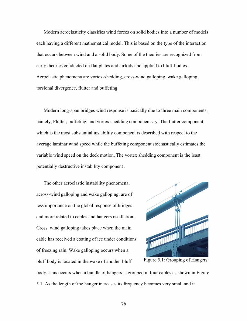
Modern aeroelasticity classifies wind forces on solid bodies into a number of models

each having a different mathematical model. This is based on the type of the interaction

that occurs between wind and a solid body. Some of the theories are recognized from

early theories conducted on flat plates and airfoils and applied to bluff-bodies.

Aeroelastic phenomena are vortex-shedding, cross-wind galloping, wake galloping,

torsional divergence, flutter and buffeting.

Modern long-span bridges wind response is basically due to three main components,

namely, Flutter, buffeting, and vortex shedding components. y. The flutter component

which is the most substantial instability component is described with respect to the

average laminar wind speed while the buffeting component stochastically estimates the

variable wind speed on the deck motion. The vortex shedding component is the least

potentially destructive instability component .

The other aeroelastic instability phenomena,

across-wind galloping and wake galloping, are of

less importance on the global response of bridges

and more related to cables and hangers oscillation.

Cross–wind galloping takes place when the main

cable has received a coating of ice under conditions

of freezing rain. Wake galloping occurs when a

bluff body is located in the wake of another bluff

body. This occurs when a bundle of hangers is grouped in four cables as shown in Figure

5.1. As the length of the hanger increases its frequency becomes very small and it

Figure 5.1: Grouping of Hangers

76

becomes vulnerable to wind. Those hangers in the windward are susceptible to vortex-

induced motion and will shed a wake that extends to the leeward hangers, which become

susceptible to wake galloping.

This phenomenon might also be of interest in the case of two bridge decks being

closely separated and located nearly at the same level. The wake of the upstream deck

might induce violent oscillation in the downstream one. A New Tacoma Narrows Bridge

is currently under construction next to the exiting one. A wind tunnel experiment is done

by Rowan Williams Davies & Irwin Inc. (2003) to check the galloping effect. The report

concluded the safety of both bridges. The following is a summary of the most important

three aeroelasticity phenomena vortex-shedding, self-induced vibration, and buffeting.

5.4.1 Vortex-shedding The very first observation on flow-structure-interaction was published by Vincenz

Strouhal in 1878. Strouhal observed that there is a relation between the natural frequency

of an Aeolian wire and its vibration frequency induced by wind flow. He concluded that

the sound of the wire would be substantially magnified when the frequency of the

vibration approaches the natural frequency of the wire. Strouhal came up with a non-

dimensional quantity, known as Strouhal Number (S) that concludes the regularity of

vortex-shedding phenomena of a bluff body.

UDNS S= 5.1

77

Where Ns is the frequency of a full vortex shedding cycle, that is, the shedding

frequency, D is the characteristic dimension of the body projected on a plane normal to

the laminar oncoming flow velocity, U. Strouhal Number is constant for certain-cross

sectional shapes.

Wake behavior in certain Reynolds number range is found to be remarkably regular.

Benard, in1908,and Theodore Von Karman, in1911, reported the behavior of vortex

shedding behavior of flow around a two-dimensional cylinder. They investigated the

separation of the flow around the cylinder and noticed alternating vortices shed from the

cylinder and form a clear recurring “vortex trail” downstream. The fine details behind

this phenomenon were not quite investigated and many theoretical and experimental

studies were conducted to find an explanation.

Abstractly, vortex-shedding is a phenomenon that takes place subsequent to the

separation of the boundary layer as a result of the interaction between oncoming fluid

flow and a bluff body. Depending on the bluff body’s shape at certain Reynolds number,

the boundary layer might experience unsteady separation that leads to a repeating pattern

of eddies, called the Von Karman vortex trail.

For a certain shape, the mechanism of vortices is function of Reynolds number. For

example the flow around a cylinder looks symmetric and with no separation in the

boundary layer at Re ≈ 1. Separation is initiated at Re ≈ 20, where two symmetric eddies

start forming next to the solid body and extend downstream. Up to this limit, drag force is

78

mainly generated due to the viscosity of the fluid and the skin friction of the solid body.

Pressure around the solid body is symmetric, and hence the lift force is negligible. The

two eddies grow the Reynolds number increases, Re ≈ 30 to 5000, and the flow starts

shedding a staggered, well-defined, alternating arrangement of vortices that travel

downstream at a velocity fairly less than that of the surrounding fluid. Transition to

turbulence in the wake and large separation in the shear boundary layer downstream

occur as the Reynolds number increases, Re ≈ 5,000 to 200,000. In this range three

dimensional patterns start forming and transition to turbulent flow occurs in the wake as

the Reynolds number decreases along the wake from that closer to the cylinder surface to

that downstream, and the clear vortex-shedding disappears. In high Reynolds number

flow, Re > 200,000, the wake narrows substantially resulting in considerable reduction in

the drag. Analogues vortex-shedding behaviors are also observed for other types of bluff

bodies, such as, triangles, squares, prisms and I- and H-shape sections.

When vortex shedding takes place the positive/negative pressure distribution around

the body alternates with time. This creates oscillatory motion across the flow. The

frequency of the shedding, Ns as shown in Equation 5.1, determines the frequency of the

solid body oscillation. If the shedding frequency matches the natural frequency of the

body resonance takes place. The dynamic system is only a function of the across flow

degree of freedom. If other degrees of freedom are included in the system, flutter will

take place. Distinction between vortex-shedding motion and flutter will be discussed in

the self-induced forces section. For a high Reynolds number, the Strouhal number could

79

be averaged and considered to be constant for a specific shape. It is found that for

cylinders Strouhal number is 0.2 and for an I-beam it is around 0.12.

Experimental tests for different bluff bodies showed that at a certain range of

Reynolds number depending on the tested shape the frequency of shedding remains

unchanged and equal to the natural frequency of the structure. This is known as the Lock-

in phenomena, where the stored energy equals the damped energy, and thus excessive

response is manifested.

Vortex shedding vibration could be ignored in most of the current long-span

instability problems. Vortex-shedding induced vibration is significant when the deck

section has blunt shape and has relatively low structural frequency. However, some

earlier bridges such as the Original Tacoma Narrows Bridge were very susceptible to

vortex-induced forces as they have a very slender low frequency H-shape deck.

Vortex shedding force is important to be checked for the local instability of individual

elements, such as beam, truss or cable elements. Generally, vortex-induced forces of

individual elements, such as the I-beam, T-beam and L-beam, add significant change to

the stored energy in the whole structure which may turn the load estimate by building

codes to be less conservative, Grant and Barnes (1981). Hangers and cables are the most

susceptible structural elements for vortex-induced forces. Hangers located in the wake of

other hangers will be more vulnerable to high vibration amplitudes. This depends on the

angle of attack of the wind and the spacing between the hangers, Cigada et. al. (1997). In

80

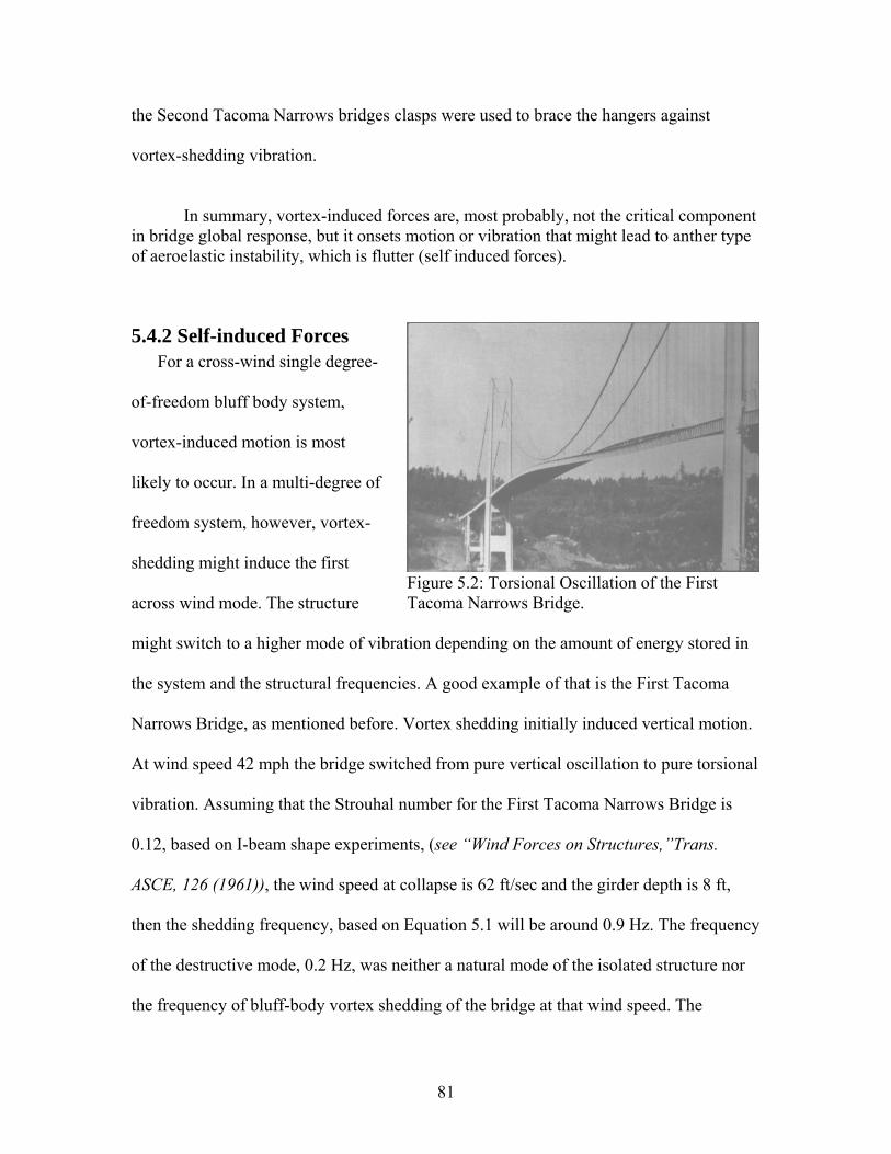
the Second Tacoma Narrows bridges clasps were used to brace the hangers against

vortex-shedding vibration.

In summary, vortex-induced forces are, most probably, not the critical component

in bridge global response, but it onsets motion or vibration that might lead to anther type of aeroelastic instability, which is flutter (self induced forces).

5.4.2 Self-induced Forces For a cross-wind single degree-

of-freedom bluff body system,

vortex-induced motion is most

likely to occur. In a multi-degree of

freedom system, however, vortex-

shedding might induce the first

across wind mode. The structure

might switch to a higher mode of vibration depending on the amount of energy stored in

the system and the structural frequencies. A good example of that is the First Tacoma

Narrows Bridge, as mentioned before. Vortex shedding initially induced vertical motion.

At wind speed 42 mph the bridge switched from pure vertical oscillation to pure torsional

vibration. Assuming that the Strouhal number for the First Tacoma Narrows Bridge is

0.12, based on I-beam shape experiments, (see “Wind Forces on Structures,”Trans.

ASCE, 126 (1961)), the wind speed at collapse is 62 ft/sec and the girder depth is 8 ft,

then the shedding frequency, based on Equation 5.1 will be around 0.9 Hz. The frequency

of the destructive mode, 0.2 Hz, was neither a natural mode of the isolated structure nor

the frequency of bluff-body vortex shedding of the bridge at that wind speed. The

Figure 5.2: Torsional Oscillation of the First Tacoma Narrows Bridge.

81

justification lays in understanding flutter, where the aerodynamic forces and the excited

structural frequency are mutually developing to an extent where instability takes place at

a combination of modes of vibration.

Flutter is classified into different categories. Classical flutter is originally recognized

in aerospace applications and applied to thin airfoils, and later applied to long-span

bridges. It indicates an aeroelastic phenomenon in which two degrees of freedom of a

structure, mainly torsional and vertical translation, couple in a flow-driven, unstable

condition. The coupling of modes is the characteristic sign of the classical flutter. Other

types of flutter are stall flutter or single-degree-of-freedom flutter, where oscillation of

the solid part is driven by nonlinear characteristics of lift or torsional forces, such as,

sudden loss of lift. In the structural sense, flutter is analogous to buckling, where a small

magnitude of perturbation could be sufficient to be the incipient of the critical mode. The

analytical models developed to solve the flutter problem assume oncoming wind in a

steady-state condition.

5.4.3 Buffeting Buffeting force is the aeroelastic component that accounts for the unsteady wind

component to the instability of slender structures in wind. The fundamental ideas to

estimate buffeting of line-like structures by atmospheric turbulence are set up by

Liepmann (1952) and Davenport (1961). Most of the theories are developed based on

statistical models to synthesize a random periodic function which simulates the

82

fluctuating wind component. Several assumptions and simplifications are used to

simplify the buffering analysis of line-like structures. These assumptions are:

a) The oscillations of the structure in each responding mode are very small and, i.e.,

aerodynamic behavior of the structure is linear; b) The squares and products of the

velocity fluctuations are negligible with respect to the square of the mean velocity and

c) The static force coefficients are independent from the frequency in the range

considered. Thus it is assumed that the buffeting force is based on a quasi-steady theory

and is not function of frequency as the case with the flutter force. This inconsistency

requires superimposing the buffeting forces and the self-exited forces simultaneously

assuming harmonic response of the structure to give the total aerodynamic force.

Buffeting response of suspension bridges is not discussed in this research and only

flutter analysis is considered. This does not necessarily imply that the critical response is

underestimated or that the critical wind speed is overestimated. In fact tests done on an I-

beam, a cylinder and a square sections show that increasing the turbulence intensity of

the oncoming wind diminishes the amplitude of oscillation of the bluff-bodies at a given

average wind velocity, Barriga-Rivera (1973).

Diana et al (1993) concluded, based on quasi-static analysis, that for a box shape deck

the effect of turbulence is correlated to the degree of nonlinearity of the wind derivative,

where a sudden divergence in the angle of attack due to flutter instability, might cause

change in the response due to high degree of wind turbulence intensities. In some cases

the turbulence of wind, when considering the sign couple derivatives, reduces the

83

effective torsional stiffness of the bridge deck, causing excessive rotational displacement

at flutter. It does however damp out the torsional acceleration response. Diana et al

(1993) also concluded that in the case of low turbulence flutter velocity does not change.

In case of strong turbulence with more than 0.2 turbulence intensity, it is difficult to settle

the flutter velocity because oscillation amplitudes are already high because of large wind

force.

5.5 Analytical Models of Flutter Motion-induced, or self-excited, forces play an important role in the design of

suspension bridges. When wind velocity reaches a speed at which the input energy from

the self-induced motion is equal to the dissipated energy by mechanical damping, flutter

occurs and the wind speed is called critical flutter wind velocity.

Flutter analysis could be accomplished using experimental and/or analytical

techniques. Wind tunnel is the standard experimental method where a prototype

resembling the whole structure is modeled and tested. Analytical methods are derived

based on time and frequency domains. The frequency domain method is adopted by most

researches since it requires less computational effort than the time domain analysis

method. Thus it became the attractive traditional method in the absence of efficient

computer resources, Scanlan (1988). To provide reduced computational efforts,

researchers used to consider multi-mode analysis instead of full-mode analysis, also

known as the direct method. In the multi-mode analysis modal superposition is employed

to sum up the effect of dynamic properties and represent coupling between frequencies.

84

Full-mode analysis requires explicit representation of all the degrees-of-freedom required

along the structure, and then solving the equation of motion to fine the critical flutter

condition.

Several modes of vibration are involved in suspension bridges. Coupling of two

modes namely the vertical and the torsional modes usually takes place when the structure

starts to reach its critical vibration frequency. Multi-mode behavior, with more than two

degrees-of-freedom, becomes more significant with the increased center-span length.

Multi-mode flutter is likely to occur when the location of the maximum deflections of

two modes coincide with each other. Most of the studies suggest coupling of the vertical

and the torsion modes of vibration.

Ge and Tanaka (2000) proposed a study that investigates these issues and provides a

numerical approach for multi-mode and full-mode aerodynamic flutter analysis. There

are two issues associated with the multi-mode frequency domain analysis where the

assumption includes dynamic coupling between natural modes and the self-excited

aerodynamic forces. The first issue involves the number and kind of natural modes

participating in the instability of the structure. The second issue involves the mode

combination which is only an approximate expression of flutter and thus the result of the

modal superposition will not necessarily be always accurate. Still the results of both types

of analysis are sufficiently close considering the accuracy required in engineering

85

applications. Multi-mode analysis is adopted in the research. The following is a

discussion for the solution process.

5.5.1 Equation of Motion The equation of motion of a bridge with a two-degree-of-freedom section could be

written as follows:

aehh Lhkhchm =++ &&& 5.2-a

aeMkcI =++ ααα αα &&& 5.2-b

where: m is the mass per unit length, I is the mass moment of inertia per unit length,

cα and ch are the coefficients of viscous damping, h and α are the vertical and the

rotational displacements, as shown in Figure 5.3, and Lae and Mae are the self-exited

aerodynamic lift and Moment forces about the rotational axis per unit span, respectively.

The above equation requires that the center of mass be located in the vertical plane of

the center of rotation. This is typical in suspension bridges where the deck is symmetric

about its vertical axis. It is, however, not necessary that the two centers match along the

vertical axis. The above equation can also be rewritten as a function of frequency:

( ) aehhh Lhhhm =++ 2ωωξ &&& 5.3-a

( ) aeMI =++ αωαωξα ααα2&&& 5.3-b

Where: ξh and ξα are damping ratios-to-critical, and ωh and ωα are the natural circular

frequencies in the h and α degrees-of-freedom, respectively.

86

For a certain wind speed, the force functions, Lae and Mae, are function of time,

frequency and response as discussed in the coming section. The solution of this equation

is not easy, as in the Duhamel integration or in other classical time domain analysis. The

solution is in both the frequency and the time domain with one domain having to be

transformed to the other. The next section discusses the solution of the equation of

motion of the self-induced forces.

5.5.2 Self-induced Forces For steady motion of thin symmetrical airfoil across a uniform airflow at an angle of

attack α, the lift force based on the potential flow theory is given by:

αdα

dCBρUL L221= 5.4

where, U is the incoming flow velocity with no turbulence and B is the plate width.

CL is the coefficient of lift per unit span, dCL/dα is the coefficient of lift gradients.

Although flutter in its details involves nonlinear aerodynamic behavior, it has been

possible in a number of instances to treat the problem successfully by linear analytical

approaches. The justification for the linearization of flutter analysis is that the structure

response is usually treatable as linearly elastic and follows exponentially modified

sinusoidal oscillation. Moreover, the stable and the unstable regimes are separated by an

incipient condition that may be treated as having small amplitude to onset it, Simiu and

Scanlan (1996).

87

Scanlan and Tomko (1971) established the fundamentals of aerodynamic flutter of

bridge decks. Sinusoidal motion is assumed to obtain the components of the aerodynamic

flutter forces as indicated by:

⎟⎟⎟

⎠

⎞

⎜⎜⎜

⎝

⎛+++++=

•••

BpHK

UpKH

BhHKαHK

UαBKH

UhKHBρUL *

62*

5*4

2*3

2*2

*1

221

ae 5.5-a

⎟⎟⎟

⎠

⎞

⎜⎜⎜

⎝

⎛+++++=

•••

BhPK

UhKP

BpPKαPK

UαBKP

UpKPBρUD *

62*

5*4

2*3

2*2

*1

221

ae 5.5-b

⎟⎟⎟

⎠

⎞

⎜⎜⎜

⎝

⎛+++++=

•••

BpAK

UpKA

BhAKαAK

UαBKA

UhKABρUM *

62*

5*4

2*3

2*2

*1

2221

ae 5.5-c

where: h, p and α are the vertical, lateral and twist deflections, ρ is the air density, U

is the mean cross-wind velocity, B is the deck width, K=Bω/U is the reduced frequency,

and ω is the circular frequency of oscillation. Hi, Pi and Ai are flutter derivatives, which

are defined in the next section. The dot superscript indicates the first derivative with

respect to time. Figure 5.3 shows the aeroelastic forces and their corresponding

displacement for a three-degree-of-freedom bridge section.

Coupling of mode of vibration is significant in flutter analysis of long span bridges.

Katsuchi H. and et al (1998), conducted multi-mode frequency domain flutter and

buffeting analysis on the Akashi-Kaikyo Bridge, in Japan. The study considered coupling

of modes to determine the aeroelastic response. It was concluded that the lateral flutter

derivatives are significant in initiating flutter for very long-span bridges.

88

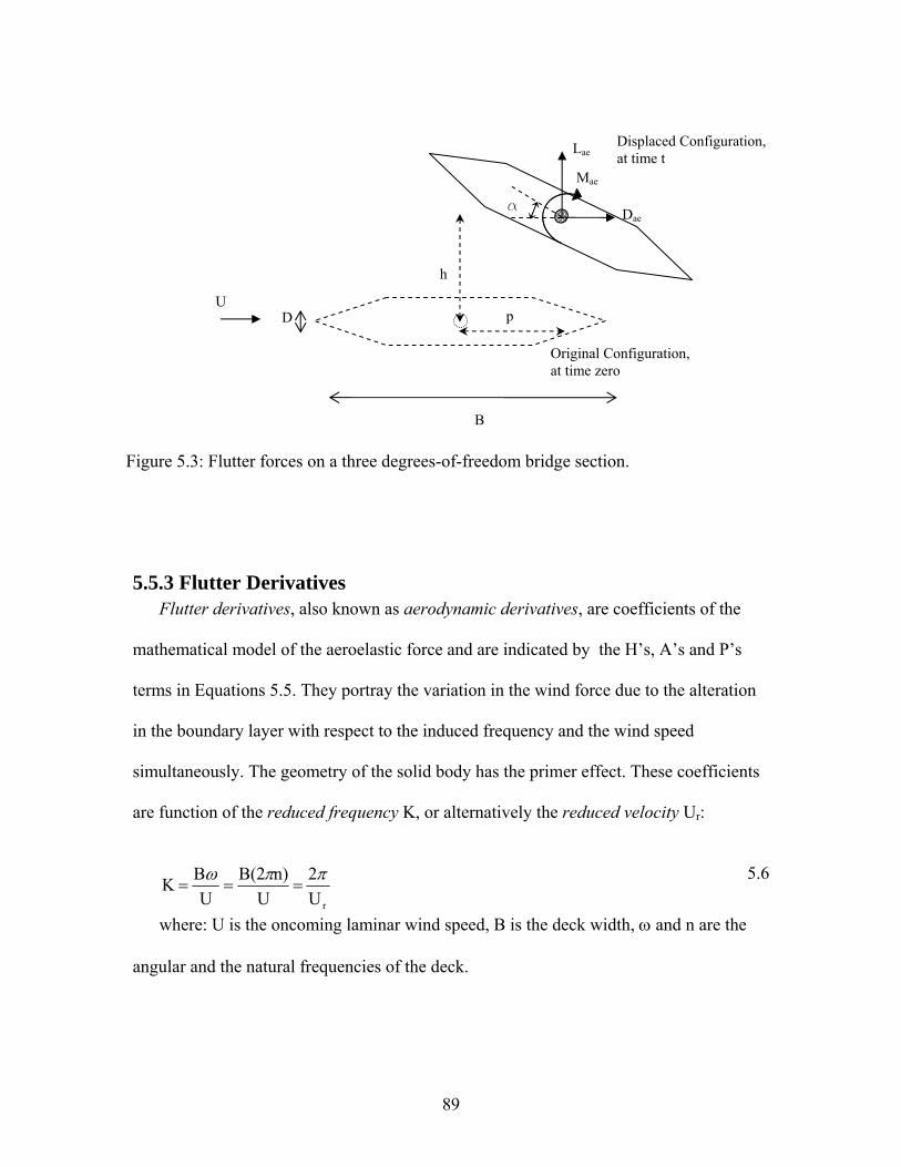
Displaced Configuration, Lae at time t Mae

Figure 5.3: Flutter forces on a three degrees-of-freedom bridge section.

5.5.3 Flutter Derivatives Flutter derivatives, also known as aerodynamic derivatives, are coefficients of the

mathematical model of the aeroelastic force and are indicated by the H’s, A’s and P’s

terms in Equations 5.5. They portray the variation in the wind force due to the alteration

in the boundary layer with respect to the induced frequency and the wind speed

simultaneously. The geometry of the solid body has the primer effect. These coefficients

are function of the reduced frequency K, or alternatively the reduced velocity Ur:

rU2

Un)B(2

UB K ππω

=== 5.6

where: U is the oncoming laminar wind speed, B is the deck width, ω and n are the

angular and the natural frequencies of the deck.

D

B

Dae a

h

U p

Original Configuration, at time zero

89

Research has recently been conducted to extract wind derivatives based on theoretical

bases. Most of the recent advances done in this regard are adopt from aeronautical

engineering. Traditionally, aerofoil or extremely thin-plate were the typical sections to be

studied. The understanding of airfoil flutter and its derivatives in incompressible flow

was reached through the potential-flow theory, done independently by Kussner and

Theodorsen, and then applied to a flat plate.

Wagner (1925) proposed a formulation for the left force as a function of time for a

theoretical flat plate airfoil due to an impulsive change in the angle of attack. Wagner

used superposition integral to estimate the indicial lift function. Theodorsen (1935),

however, determined the lift and the moment forces based on sinusoidal oscillating airfoil

in a uniform airflow. Theodorsen introduced a complex circulation function, which is

function of the frequency of oscillatory motion (refer to Appendix E)

Bridge engineering researchers investigated the possibility of applying the

Theodorsen function on bluff bodies. Although it is found that there is a fairly close

parallelism in form between the problems of the aerodynamic instability of suspension

bridge decks and flutter of airfoils, the latter should not be carried beyond its logical

usefulness and must be used only as a guide in the study of bridge flutter, Scanlan et. Al

(1971). Early experiments on extracting flutter derivatives for bridge decks were

conducted by Ukeguchi, Sakata, and Nishitani (1966).

90

For a full mode analysis there are six lateral terms for each of the (P’s) (H’s) and

(A’s) for flutter derivatives, as shown in Equations 5.5. These coefficients can be

extracted using sectional wind tunnel tests such that only a representative segment along

the span length is modeled and tested. The lateral wind coefficients are unlike other

flutter coefficients since they are found to be correlated to the static drag coefficient.

Thus, they do not need to be extracted using oscillating model in wind tunnel.

The following is a discussion of the flutter derivatives. Extraction methods are briefly

discussed. A comprehensive discussion of the behavior and the significance of the flutter

derivatives is incorporated. Examples, based on pervious studies are included to help in

defining the range and the shape of the aerodynamic derivative curves. The results of the

coming discussion are employed to synthesize flutter derivative curves for closed-grates

stiffened-truss deck. This will be utilized in the flutter analysis of the Second Tacoma

Narrows Bridge wind response analysis.

5.5.3.1 Extracting Flutter Derivatives Aerodynamic derivatives of bluff bodies can be extracted from wind tunnel tests,

using a prototype section of the superstructure. There are three procedures for

accomplishing such a task:

1) Conducting vibration tests by giving prescribed vertical and torsional

displacements to the bridge deck and then the aerodynamic derivatives are determined

based on the transient behavior that occurs after releasing the bridge deck.

91

2) Applying the forced oscillation and using pressure measurements at number of

pressure taps on the model.

3) Conducting buffeting tests where the behavior of the superstructure is observed

under variable wind velocities.

Scanlan et al (1971) introduced an experimental setup with the basic theory and

technique needed to extract flutter coefficients experimentally. The research tested a

standard airfoil, NACA 0012, and compared the results with the theoretical values based

on the Theodorsen function and exponentially modified sinusoidal harmonic response.

Flow regime is assumed to be a low-speed low-turbulence incompressible flow. Figure

5.4 shows the results obtained by the experiments and the corresponding theoretical

curve. Note that discrepancies from the theory exist. The experimental A2 coefficient is

reduced by a factor equal to 4.54, to match with the theory. Experimental values of H1

and H2 show considerably deviation from the Theodorsen function. The disagreement in

H1 is due to some limitation in the proposed experimental procedure as the torsional

motion is initially blocked rather than permanently restrained. This causes the torsional

motion to increase due to the inherently large coupling between the vertical and the

torsional motion. This affects the calculation of H2 and H3 as well since both of them are

function of H1.

Experimental computations of the aerodynamic derivatives involve some

uncertainties that influence the quality of the results. Curve fitting seems acceptable, but

92

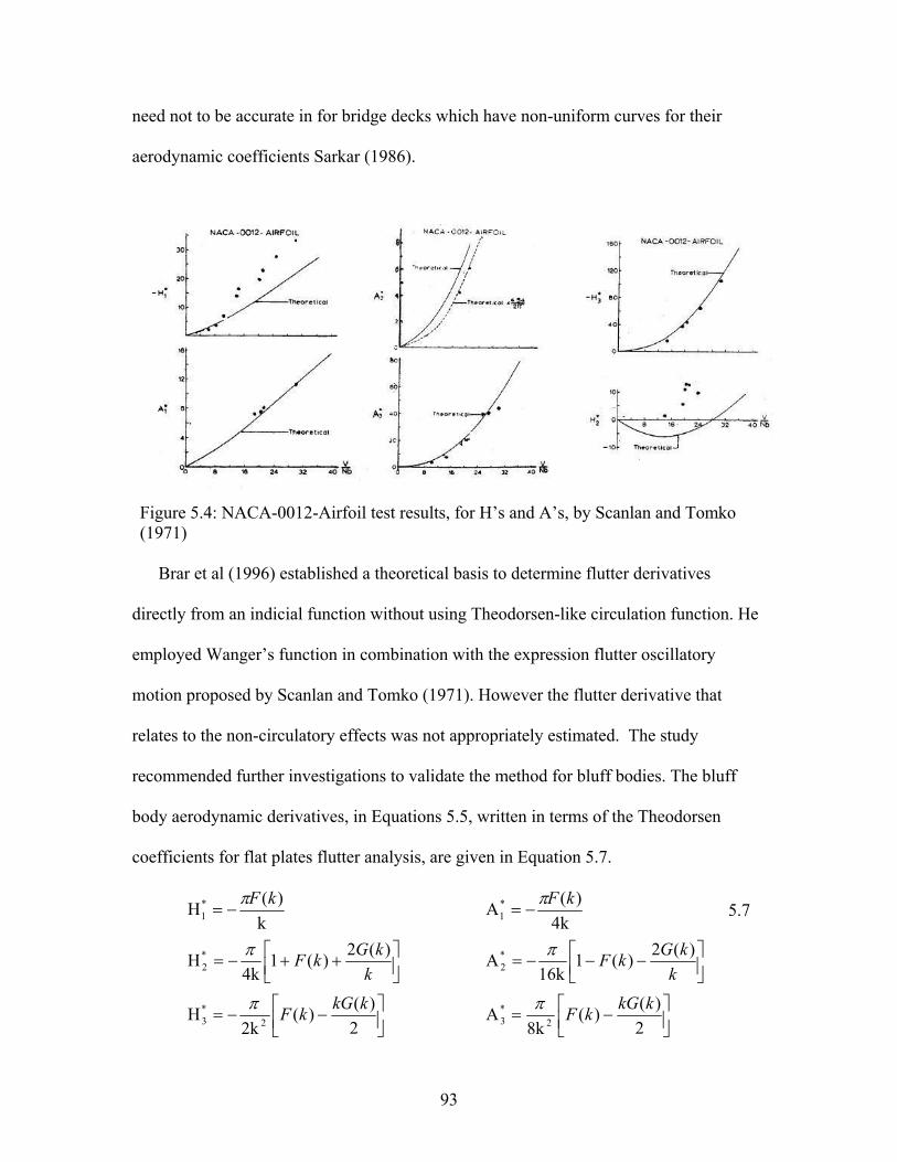
need not to be accurate in for bridge decks which have non-uniform curves for their

aerodynamic coefficients Sarkar (1986).

Figure 5.4: NACA-0012-Airfoil test results, for H’s and A’s, by Scanlan and Tomko (1971)

Brar et al (1996) established a theoretical basis to determine flutter derivatives

directly from an indicial function without using Theodorsen-like circulation function. He

employed Wanger’s function in combination with the expression flutter oscillatory

motion proposed by Scanlan and Tomko (1971). However the flutter derivative that

relates to the non-circulatory effects was not appropriately estimated. The study

recommended further investigations to validate the method for bluff bodies. The bluff

body aerodynamic derivatives, in Equations 5.5, written in terms of the Theodorsen

coefficients for flat plates flutter analysis, are given in Equation 5.7.

k)(H*

1kFπ

−= 4k

)(A*1

kFπ−=

⎥⎦⎤

⎢⎣⎡ ++−=

kkGkF )(2)(1

4kH*

2π ⎥⎦

⎤⎢⎣⎡ −−−=

kkGkF )(2)(1

16kA*

2π

⎥⎦⎤

⎢⎣⎡ −−=

2)()(

2kH 2

*3

kkGkFπ ⎥⎦⎤

⎢⎣⎡ −=

2)()(

8kA 2

*3

kkGkFπ

5.7

93

⎥⎦⎤

⎢⎣⎡ +=

kkG )(21

2H*

4π

kkG )(

4A*

4π

=

Gu M. et. al. (2000) adopted spring-suspended section model and proposed a method

to extract flutter derivatives based on Scanlan’s formulation. The study consolidates the

damping and stiffness matrices of the governing equation of motion into a damping and

stiffness matrices of the wind-bridge system. That is, the response variables in the self-

excited wind force function are combined with the damping and stiffness terms of the

structure. The response of the bridge is approximated by the exponential function. Least

square method is used to optimize the error based on the iterative procedure. The wind

derivative is then computed based on the damping and stiffness matrices of the wind-

bridge system and those of the structure itself. The wind derivatives obtained by the study

were positively comparable with those obtained by Scanlan’s theory.

Extraction of the lateral flutter derivative is done by wind tunnel experiments. It is

then correlated to the static wind coefficients, namely, the drag coefficient Singh et al

(1996). The following relations given in equation 5.8 are suggested to find the first three

lateral flutter derivatives:

D*

1 CK2P −= 5.8-a

w

D*2 d

dCK1P

α−= 5.8-b

w

D2

*3 d

dCK1P

α−= 5.8-c

where: K is the reduced frequency, CD is the static drag coefficient, and αw is the

angle of incident of the wind.

94

The flutter derivatives theory is conceptually, well established. Experimental research

done by Scanlan and other investigators are acceptable to evaluate the parameters of the

linearized system of aeroelastic forces. A procedure to determine all of the 18 flutter

derivatives in a single test, at each reduced frequency level, using three-degree-of-

freedom suspension and the application of a state-of-the-art system identification

technique has been developed by Sarkar et al. (1994).

The ongoing research of evaluating the values of flutter derivatives using analytical

models, such as computational fluid dynamics are still under investigation. Thus,

experimental tools are still essential to validate the new analytical method.

5.5.3.2 Parametric Analysis Parametric studies have been conducted to examine the trends of flutter derivatives

with respect to the bridges physical properties. These include deck shapes and

configurations, and the wind properties such as turbulence intensity.

Scanlan and Tomko (1971) extended their experiments to extract the flutter

derivatives for different types of representative suspension bridge decks, including

closed-box, H-sections and stiffening truss. The plots shown in Figure 5.5 are some

selected results from the experiments done on truss-stiffened cross sections.

95

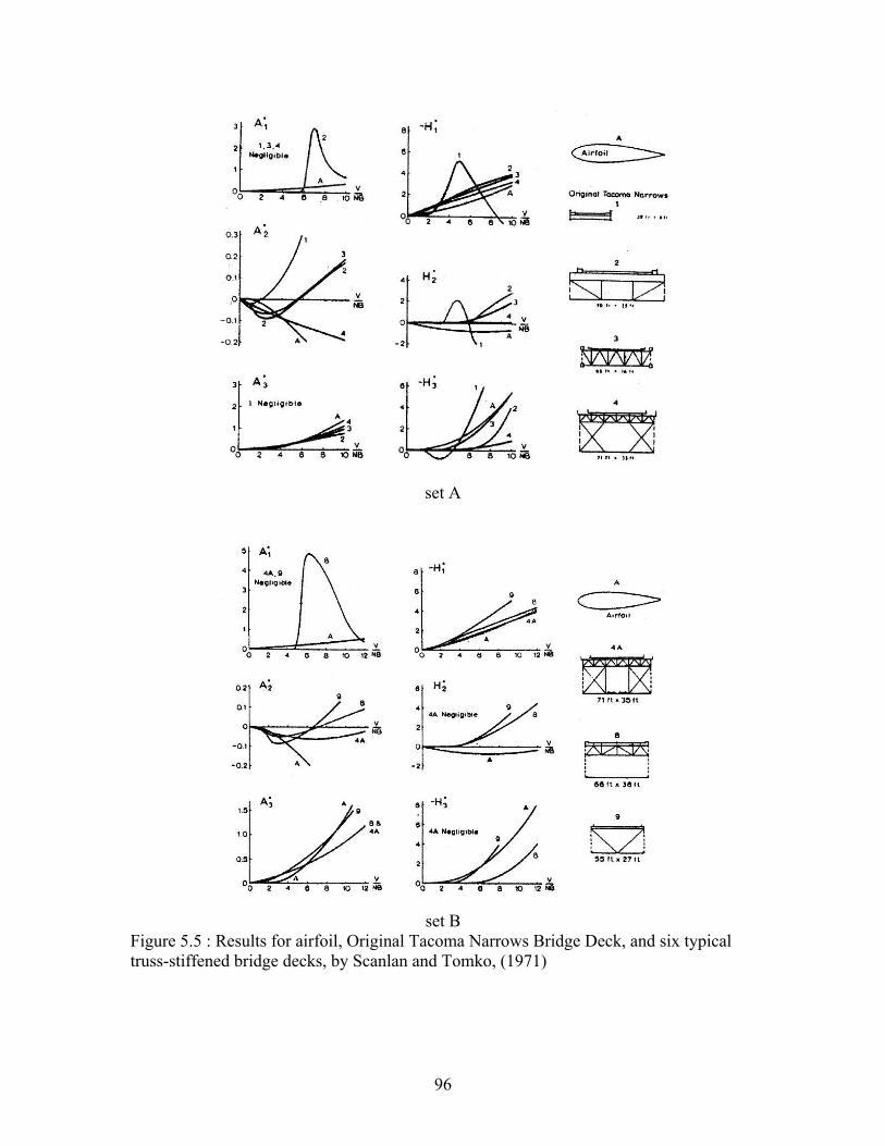
set A

set B

Figure 5.5 : Results for airfoil, Original Tacoma Narrows Bridge Deck, and six typical truss-stiffened bridge decks, by Scanlan and Tomko, (1971)

96

The aerodynamic coefficients depend on the ratio of the wind speed and the

frequency excited. They are however, independent of damping. The curves shown in

Figure 5.5 are function of the reduced velocity, which is the ratio of the oncoming

laminar wind speed to the frequency excited, in Hertz, times the width of the

superstructure. The shape or the magnitude of the curves is solely affected by the

geometrical configuration of the model.

If fluid-structure-interaction is considered, the wind derivatives could be

contemplated as the reflection of the interaction of the wind boundary layer and the

excited solid body. For example, in Figure 5.5 – set A, curve number one is for the

original Tacoma Narrows Bridge deck is remarkably different from the other curves. This

is due to the vortex-shedding behavior in the wind boundary layer, associated with the

bridge motion, which has a significant effect on H-shape sections. However, this

phenomenon is insignificant in the truss-stiffened cross sections shown. The curves are

derived assuming that the lift force and the vertical deflection are both positive

downward, and the twisting motion and moment are both positive with the windward

edge upward. If this sign convention is reversed the terms H2, H3, A1 and A4 should be

reversed in sign. This would not affect the flutter analysis results, as discussed later in

this chapter. The following is a discussion of the first three aerodynamic coefficients for

left Ai and moment Hi and Ai (i=1, 2 and3):

The H1 Coefficient represents the response of the vertical motion with the torsional

degree –of freedom initially blocked, i.e., (α (0) = 0). The figure shows that all bridges

97

with open-truss stiffened decks are close in response to an airfoil. However, the H-shape

section, with its considerable side girders, diverts from the airfoil response. In most cases,

the airfoil results are the lower bound, with a negative value, for the other opened truss-

stiffened bridges.

The H2 and H3 coefficients represent the effect of the torsional oscillation on the

buildup or decay of the vertical motion. For an example it is observed from experiments

that for an H-shape the increase in the torsional oscillation frequency is associated with

reduction in the vertical oscillation. This can be depicted by these two coefficients. For an

example, curve 1 in Figure 5.5 increases with the increase of the reduced speed. Then it is

swiftly reduced in the negative value causing a sudden reduction in the left force and thus

a sudden increase in the torsional oscillatory frequency to converge in values with the

structural torsional frequency. This behavior is not exhibited by other deck shapes.

For open truss-stiffened decks the H2 lies well above the airfoil curve and is always

positive. This implies the opposite behavior exhibited by the H-shape deck of the

Original Tacoma Narrows Bridge. The H3 coefficient, however, shows similar behavior

to the H-shape deck at a high reduced frequency. If these two aerodynamic coefficients

reduce the aerodynamic vertical force at a high reduced wind speed, it is most probable

that coupling between the heaving and torsional flutter will occur.

The effect of the vertical motion on the torsional flutter usually is not significant as

shown by the A1 curves of Figure 5.5. This coefficient may contribute to the response

98

when strong coupling between the two modes takes place at a certain frequency. At that

point the term A1 increases suddenly and then decreases to a low value, as shown in

curve 1.

Generally A1 has a relatively negligible contribution to the flutter condition for most

of the bridge decks investigated in the literature. The effect of the A1 coefficient on the

stability behavior appears in airfoil and thin plates such that it induces the torsional

branch-coupled flutter despite the adverse effect of A2 after the torsional motion is

initiated.

The A2 coefficient is an indication of the torsional stability of a bridge section having

the vertical motion restrained, i.e. (h(t) = 0). It is correlated to the torsional aerodynamic

damping and the possibility to have torsional divergence. The A2 curve provides a very

useful rule-of-thumb to judge and compare the aerodynamic stability, even though the

contribution of the other aerodynamic derivatives might have considerable positive

effects. A steep negative slope is an indication of torsional stability. As indicated in

Figure 5.5, the airfoil and the bridge section number 4 are the most stable sections, while

the Original Tacoma Narrows Bridge is the least stable section since the A2 coefficient is

well-correlated to the vortex-shedding effect. Flat sections or streamlined bodies have

close values to the A2 of airfoil. Moreover, grating-location, for plate-like decks with

open grates, has significant effect on the A2 value. It is found that installing the open

grates at the edge panels of the deck provides more aerodynamic stability, as shown in

Figure 5.6.

99

The A3 coefficient reflects the difference between flutter and natural torsional

frequencies, that is, the aerodynamic stiffening effect upon the critical torsional

frequency. It is found that the flutter frequency and the natural torsional frequency are

between 1% and 3%. For most of the tested sections A3 is found to be fairly close to that

of the airfoil.

It could be observed that each of the H’s and A’s coefficients portray a certain

behavior of the self-exited forces. Thus the optimal design of suspension bridge decks

could be depicted using these coefficients such that the use of an airfoil trend is the most

preferable. The challenge is to find a section, mostly a bluff body, with satisfactory

stiffness and aerodynamic properties. Different techniques are suggested to improve the

aerodynamic characteristics of suspension bridge superstructures. Such techniques are

streamlining the deck shape, as originally done in the Second Severn Bridge, installing

flaps at both edges, or introducing grates in the superstructure, as in the case of the

Second Tacoma Narrows Bridge. The Messina Strait Bridge, which is under planning in

Italy, comprises all the above three techniques. This is would make its 2.05 miles (3300

m) main span possible, Brancaleoni and Diana (1993). Several studies are done on each

of the three techniques.

The emphasis here is on studying the effect of altering the grates on the aerodynamic

response of the bridge. It is of interest, for the purpose of the case study discussed in

Chapter 6, to investigate the effect of deck grates on the aerodynamic behavior. A

100

comparison between the solid deck, open-grated deck at the sides and the Theodersen

function is essential to deduce the general trend of the aerodynamic curves. This will be

employed to synthesize wind derivative curves that substitute the deficiency in

experimental data.

Matsumoto et al (2001) conducted a parametric study, using a series of wind tunnel

tests on plate-like bridge sections with five panels. The tests are conducted with three

wind speeds of 5, 10 and 15 m/s (11.2, 22.4 and 33.6 mph). Matsumoto’s study discusses

the influence of the opening ratio and the location of grating on flutter instability based

upon their aerodynamic derivatives and flutter analysis. Different values of the opening

ratio (OR) are suggested in the test, with OR varying from 20% to 100% with 20%

increments. The different deck configurations and the aerodynamic derivatives for

grating-installed with OR=40% are shown in Figure 5.6.

For the Second Tacoma Narrows Bridge, the edge grates next to the sidewalks, are

supposed to be open as in Type 2. Note that there are dissimilarities between the bridge

deck configurations and the Matsumoto et al (2001) experiment sections. These

differences are mainly due to the number of panels and the geometry of the open-truss

stiffened decks which is different than that of the plate-like decks, as used in the

experiments. The following conclusions are to be used along with the previous discussion

to suggest a worst-case scenario for the H’s and A’s curves, relevant to the bridge

problem.

101

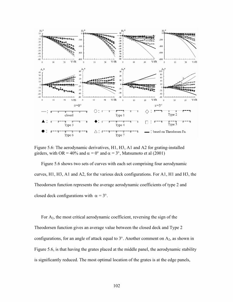
Figure 5.6: The aerodynamic derivatives, H1, H3, A1 and A2 for grating-installed girders, with OR = 40% and α = 0° and α = 3°, Matsumoto et al (2001)

Figure 5.6 shows two sets of curves with each set comprising four aerodynamic

curves, H1, H3, A1 and A2, for the various deck configurations. For A1, H1 and H3, the

Theodorsen function represents the average aerodynamic coefficients of type 2 and

closed deck configurations with α = 3°.

For A2, the most critical aerodynamic coefficient, reversing the sign of the

Theodorsen function gives an average value between the closed deck and Type 2

configurations, for an angle of attack equal to 3°. Another comment on A2, as shown in

Figure 5.6, is that having the grates placed at the middle panel, the aerodynamic stability

is significantly reduced. The most optimal location of the grates is at the edge panels,

102

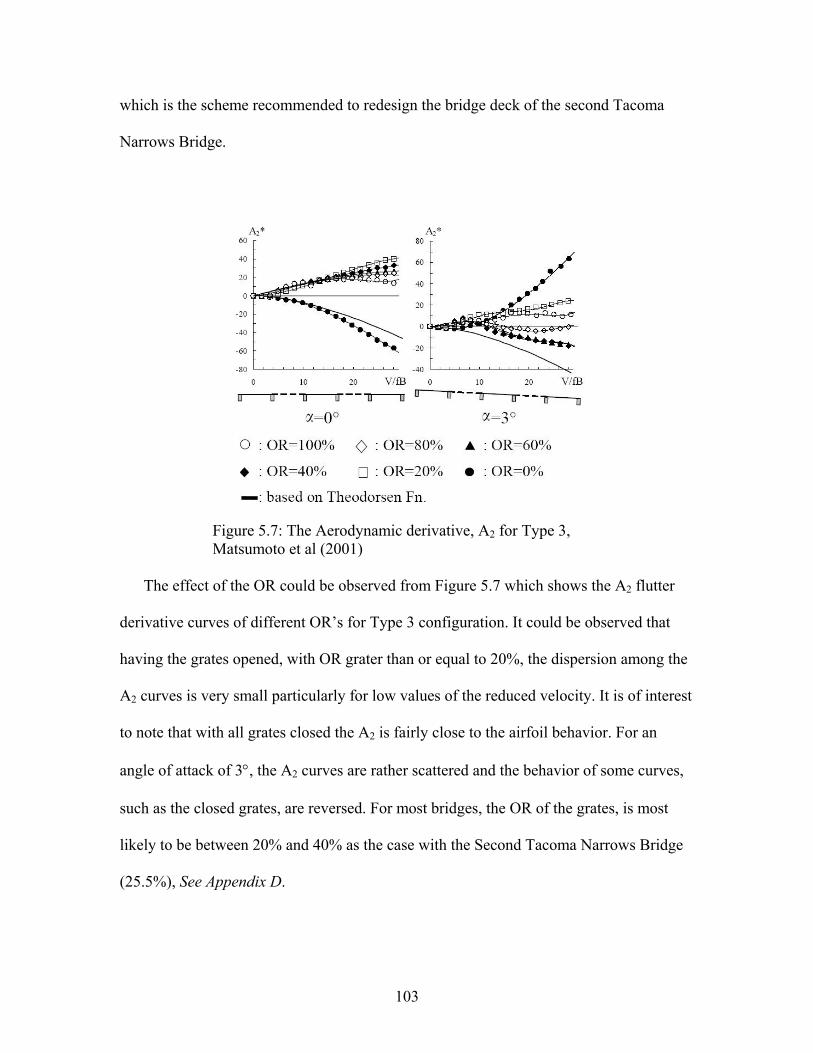
which is the scheme recommended to redesign the bridge deck of the second Tacoma

Narrows Bridge.

Figure 5.7: The Aerodynamic derivative, A2 for Type 3, Matsumoto et al (2001)

The effect of the OR could be observed from Figure 5.7 which shows the A2 flutter

derivative curves of different OR’s for Type 3 configuration. It could be observed that

having the grates opened, with OR grater than or equal to 20%, the dispersion among the

A2 curves is very small particularly for low values of the reduced velocity. It is of interest

to note that with all grates closed the A2 is fairly close to the airfoil behavior. For an

angle of attack of 3°, the A2 curves are rather scattered and the behavior of some curves,

such as the closed grates, are reversed. For most bridges, the OR of the grates, is most

likely to be between 20% and 40% as the case with the Second Tacoma Narrows Bridge

(25.5%), See Appendix D.

103

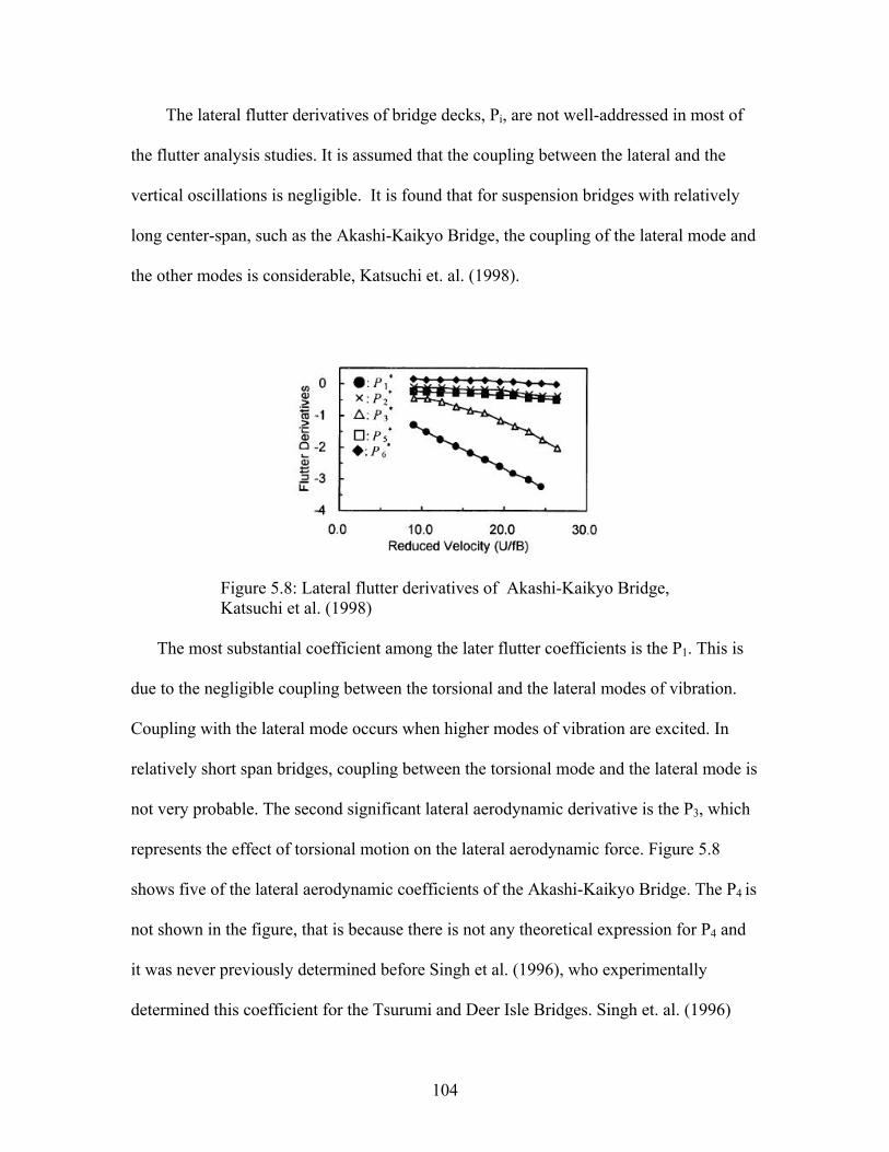
The lateral flutter derivatives of bridge decks, Pi, are not well-addressed in most of

the flutter analysis studies. It is assumed that the coupling between the lateral and the

vertical oscillations is negligible. It is found that for suspension bridges with relatively

long center-span, such as the Akashi-Kaikyo Bridge, the coupling of the lateral mode and

the other modes is considerable, Katsuchi et. al. (1998).

Figure 5.8: Lateral flutter derivatives of Akashi-Kaikyo Bridge, Katsuchi et al. (1998)

The most substantial coefficient among the later flutter coefficients is the P1. This is

due to the negligible coupling between the torsional and the lateral modes of vibration.

Coupling with the lateral mode occurs when higher modes of vibration are excited. In

relatively short span bridges, coupling between the torsional mode and the lateral mode is

not very probable. The second significant lateral aerodynamic derivative is the P3, which

represents the effect of torsional motion on the lateral aerodynamic force. Figure 5.8

shows five of the lateral aerodynamic coefficients of the Akashi-Kaikyo Bridge. The P4 is

not shown in the figure, that is because there is not any theoretical expression for P4 and

it was never previously determined before Singh et al. (1996), who experimentally

determined this coefficient for the Tsurumi and Deer Isle Bridges. Singh et. al. (1996)

104

concluded that the P4 has a “stiffening” effect on the sway motion. It is however possible,

as described in the pervious section, to at least calculate the terms P1, P2 and P3 if the

static drag coefficient is known.

Effect of turbulence is discussed by Scanlan and Lin (1978), Huston et al (1988),

Diana et al (1993) and Sarkar et al (1994). It is found that for most of the eight flutter

derivatives (A’s and H’s), the turbulent flow values differ only slightly from their smooth

flow counterparts, such that the smooth flow values seems to represent the mean values

about which the turbulent flow values fluctuate. It is found that H3 and A3 are less

influenced by the turbulence of flow as they seem to match perfectly in both cases. It is

generally determined that the effect of turbulence is very slight on the flutter derivatives,

and thus on evaluating the aeroelastic forces.

The aeroelastic behavior, represented by the flutter derivatives, is mainly driven by

the geometry of the structure. There is critical dependence of the aeroelastic behavior on

even minor details such as a deck railing Jones et al (1995).

5.5.3.3 Solving for Flutter Condition 5.5.3.3.1 Two-Degree-of-Freedom System

Wind Critical Flutter condition is the state of motion at which the zero damping is

attained and oscillation buildup is initiated. This could be noticed in wind tunnel testing,

with prototype of the whole structure as the oscillation time history diverts at a certain

wind speed and reaches resonance-like motion. Using the time history function the

critical frequency could then be identified. The mathematical solution of the flutter

105

condition is however more complicated. The following discussion is limited to the two

degree-of-freedom system such that the lateral motion is ignored.

The vertical and torsional modes that couple in the flutter vibrations are described by

Equation 5.9,

)()(),(h tzxtx mξ= 5.9-a )()(),( tqxtx mαα = 5.9-b

in which, ξm and αm are the vertical and the torsional modes that couple to produce

flutter vibration along the deck axis, x. The z(t) and the q(t) are single generalized

displacement of the vertical and the torsional displacement, respectively.

Referring to the equations of motion in section 5.4.2 and the self-induced forces in

section 5.4.3, and assuming that the vertical deflection, h, and the angular rotation, α, of

the bridge deck follow complex exponential harmonic motion given by the following

expression:

ti0eXX ω=

The solution for this equation will be in the form of ω=ω1+iω2. The ω2, if greater than

zero, represents decay of motion, and represents divergent if negative in value. Let the

critical reduced frequency Kc be the value for which ω≈ω1, that is at the critical flutter

condition (ω2≈0).

The following is defined to help in the derivation of the flutter function:

Recalling Equation 5.6,

106

UBωK =

K is the reduced frequency, U is the wind speed, B is a characteristic length, usually

the deck width, and ω is the frequency. Therefore at flutter the following is assumed

K=Kc, U=Uc and ω=ω1. For the reduced vertical structural frequency K=Kh and ω=ωh.

For the reduced torsional structural frequency K=Kα and ω=ωα.

BUts = 5.10

where s is the reduced time (or distance), and t is time. Using the chain rule, the first

derivative of a variable function of t, is as follows,

BU) (

dtds

ds) d(

dt) d( ') ( ===

•

5.11

2

2''

BU) (

dt) d() ( ==

•••

5.12

Operating Equations 5.11 and 5.12 on h and α, the equation of motion and the

aeroelastic forces, Equations 5.3 and 5.5, respectively, the equation of motion are reduced

to

⎥⎦

⎤⎢⎣

⎡+++=++

BhHKHKKH

BhKH

mBhKhKh hhh

*4

2*3

2'*2

'*1

32'''

22 ααρζ 5.13-a

⎥⎦

⎤⎢⎣

⎡+++=++

BhAKAKKA

BhKA

IBKK *

42*

32'*

2

'*1

42'''

22 ααρααζα ααα

5.13-b

Note that the left hand side and the right hand side are multiplied by B^2/U^2.

Recalling the proposed solution form of the response,

iKsti ehehh 00 == ω 5.14-a

iKstiti eee 000

~αααα ωω ===

5.14-b

107

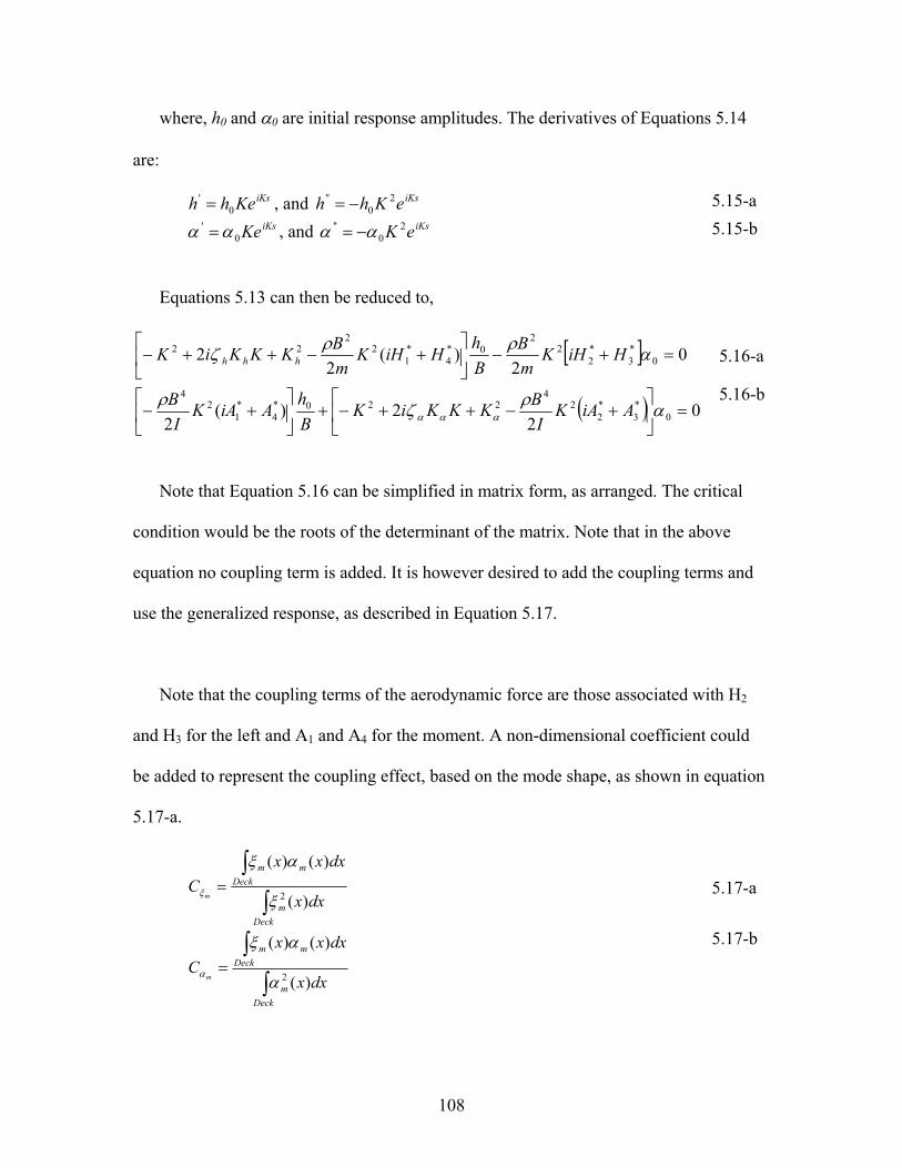
where, h0 and α0 are initial response amplitudes. The derivatives of Equations 5.14

are:

iKsKehh 0' = , and iKseKhh 2

0'' −= 5.15-a

iKsKe0' αα = , and iKseK 2

0'' αα −= 5.15-b

Equations 5.13 can then be reduced to,

[ ] 02

)(2

2 0*3

*2

22

0*4

*1

22

22 =+−⎥⎦

⎤⎢⎣

⎡+−++− αρρζ HiHK

mB

Bh

HiHKmBKKKiK hhh 5.16-a

( ) 02

2)(2 0

*3

*2

24

220*4

*1

24

=⎥⎦

⎤⎢⎣

⎡+−++−+⎥

⎦

⎤⎢⎣

⎡+− αρζρ

ααα AiAKI

BKKKiKBhAiAK

IB

5.16-b

Note that Equation 5.16 can be simplified in matrix form, as arranged. The critical

condition would be the roots of the determinant of the matrix. Note that in the above

equation no coupling term is added. It is however desired to add the coupling terms and

use the generalized response, as described in Equation 5.17.

Note that the coupling terms of the aerodynamic force are those associated with H2

and H3 for the left and A1 and A4 for the moment. A non-dimensional coefficient could

be added to represent the coupling effect, based on the mode shape, as shown in equation

5.17-a.

∫

∫=

Deckm

Deckmm

dxx

dxxxC

m )(

)()(

2ξ

αξ

ξ 5.17-a

∫

∫=

Deckm

Deckmm

dxx

dxxxC

m )(

)()(

2α

αξ

α 5.17-b

108

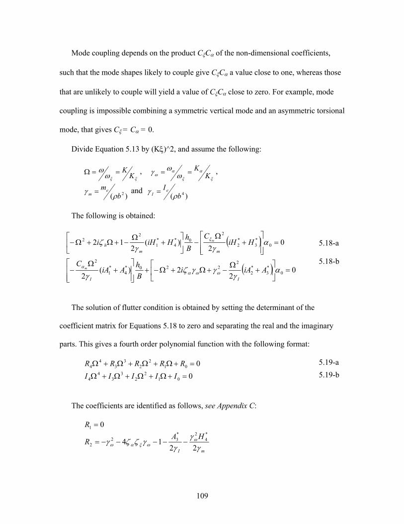
Mode coupling depends on the product CξCα of the non-dimensional coefficients,

such that the mode shapes likely to couple give CξCα a value close to one, whereas those

that are unlikely to couple will yield a value of CξCα close to zero. For example, mode

coupling is impossible combining a symmetric vertical mode and an asymmetric torsional

mode, that gives Cξ = Cα = 0.

Divide Equation 5.13 by (Kξ)^2, and assume the following:

ξξωω

KK==Ω ,

ξ

α

ξ

αω ω

ωγ KK== ,

)( 2bme

m ργ = and )( 4b

I eI ργ =

The following is obtained:

( ) 02

)(2

12 0*3

*2

20*

4*1

22 =

⎥⎥⎦

⎤

⎢⎢⎣

⎡+

Ω−⎥

⎦

⎤⎢⎣

⎡+

Ω−+Ω+Ω− α

γγζ ξ HiH

CBhHiHi

mmh

m 5.18-a

( ) 02

2)(2 0

*3

*2

2220*

4*1

2

=⎥⎦

⎤⎢⎣

⎡+

Ω−+Ω+Ω−+

⎥⎥⎦

⎤

⎢⎢⎣

⎡+

Ω− α

γγγζ

γ ωωαα AiAi

BhAiA

C

II

m 5.18-b

The solution of flutter condition is obtained by setting the determinant of the

coefficient matrix for Equations 5.18 to zero and separating the real and the imaginary

parts. This gives a fourth order polynomial function with the following format:

0012

23

34

4 =+Ω+Ω+Ω+Ω RRRRR 5.19-a

0012

23

34

4 =+Ω+Ω+Ω+Ω IIIII 5.19-b

The coefficients are identified as follows, see Appendix C:

01 =R

mI

HAR

γγ

γγζζγ ωωξαω 22

14*4

2*32

2 −−−−−=

109

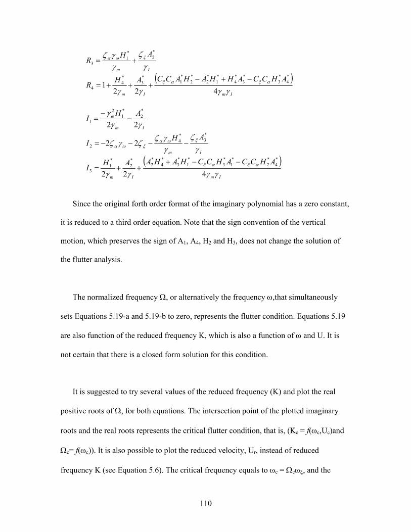
Im

AHRγ

ζγγζ ξωα

*2

*1

3 +=

( )ImIm

AHCCAHHAHACCAHRγγγγ

αξαξ

4221

*4

*3

*3

*4

*1

*2

*2

*1

*3

*4

4

−+−+++=

Im

AHIγγ

γ ω22

*2

*1

2

1 −−

=

Im

AHIγ

ζγγζ

ζγζ ξωαξωα

*3

*4

2 22 −−−−=

( )ImIm

AHCCAHCCHAHAAHIγγγγ

αξαξ

422

*4

*2

*1

*3

*1

*3

*4

*2

*2

*1

3

−−+++=

Since the original forth order format of the imaginary polynomial has a zero constant,

it is reduced to a third order equation. Note that the sign convention of the vertical

motion, which preserves the sign of A1, A4, H2 and H3, does not change the solution of

the flutter analysis.

The normalized frequency Ω, or alternatively the frequency ω,that simultaneously

sets Equations 5.19-a and 5.19-b to zero, represents the flutter condition. Equations 5.19

are also function of the reduced frequency K, which is also a function of ω and U. It is

not certain that there is a closed form solution for this condition.

It is suggested to try several values of the reduced frequency (K) and plot the real

positive roots of Ω, for both equations. The intersection point of the plotted imaginary

roots and the real roots represents the critical flutter condition, that is, (Kc = f(ωc,Uc)and

Ωc= f(ωc)). It is also possible to plot the reduced velocity, Ur, instead of reduced

frequency K (see Equation 5.6). The critical frequency equals to ωc = Ωcωξ, and the

110

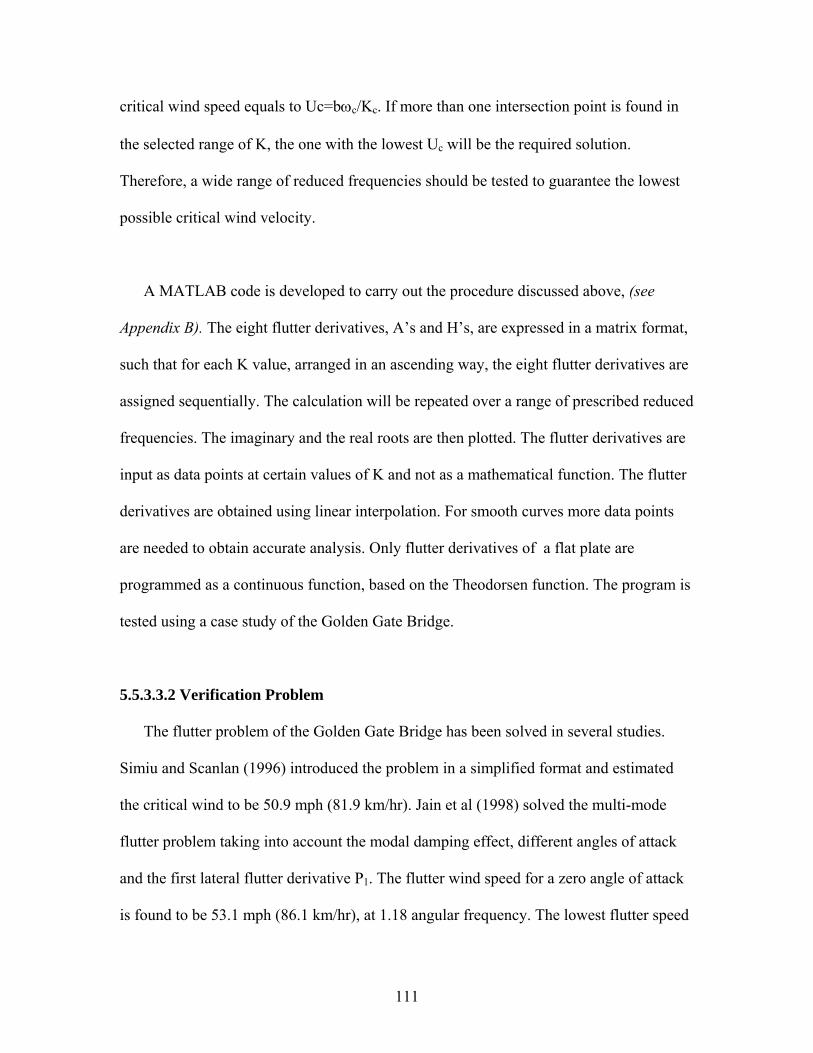
critical wind speed equals to Uc=bωc/Kc. If more than one intersection point is found in

the selected range of K, the one with the lowest Uc will be the required solution.

Therefore, a wide range of reduced frequencies should be tested to guarantee the lowest

possible critical wind velocity.

A MATLAB code is developed to carry out the procedure discussed above, (see

Appendix B). The eight flutter derivatives, A’s and H’s, are expressed in a matrix format,

such that for each K value, arranged in an ascending way, the eight flutter derivatives are

assigned sequentially. The calculation will be repeated over a range of prescribed reduced

frequencies. The imaginary and the real roots are then plotted. The flutter derivatives are

input as data points at certain values of K and not as a mathematical function. The flutter

derivatives are obtained using linear interpolation. For smooth curves more data points

are needed to obtain accurate analysis. Only flutter derivatives of a flat plate are

programmed as a continuous function, based on the Theodorsen function. The program is

tested using a case study of the Golden Gate Bridge.

5.5.3.3.2 Verification Problem

The flutter problem of the Golden Gate Bridge has been solved in several studies.

Simiu and Scanlan (1996) introduced the problem in a simplified format and estimated

the critical wind to be 50.9 mph (81.9 km/hr). Jain et al (1998) solved the multi-mode

flutter problem taking into account the modal damping effect, different angles of attack

and the first lateral flutter derivative P1. The flutter wind speed for a zero angle of attack

is found to be 53.1 mph (86.1 km/hr), at 1.18 angular frequency. The lowest flutter speed

111

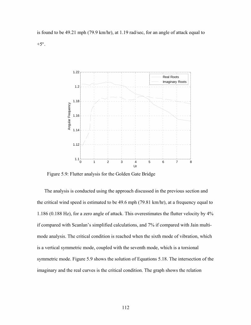
is found to be 49.21 mph (79.9 km/hr), at 1.19 rad/sec, for an angle of attack equal to

+5°.

0 1 2 3 4 5 6 7 81.1

1.12

1.14

1.16

1.18

1.2

1.22

Ur

Ang

ular

Fre

quen

cy

Real RootsImaginary Roots

Figure 5.9: Flutter analysis for the Golden Gate Bridge

The analysis is conducted using the approach discussed in the previous section and

the critical wind speed is estimated to be 49.6 mph (79.81 km/hr), at a frequency equal to

1.186 (0.188 Hz), for a zero angle of attack. This overestimates the flutter velocity by 4%

if compared with Scanlan’s simplified calculations, and 7% if compared with Jain multi-

mode analysis. The critical condition is reached when the sixth mode of vibration, which

is a vertical symmetric mode, coupled with the seventh mode, which is a torsional

symmetric mode. Figure 5.9 shows the solution of Equations 5.18. The intersection of the

imaginary and the real curves is the critical condition. The graph shows the relation

112

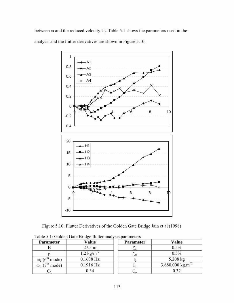
between ω and the reduced velocity Ur. Table 5.1 shows the parameters used in the

analysis and the flutter derivatives are shown in Figure 5.10.

-0.4

-0.2

0

0.2

0.4

0.6

0.8

1

0 2 4 6 8 10

A1A2A3A4

-10

-5

0

5

10

15

20

0 2 4 6 8 10

H1H2H3H4

Figure 5.10: Flutter Derivatives of the Golden Gate Bridge Jain et al (1998) Table 5.1: Golden Gate Bridge flutter analysis parameters

Parameter Value Parameter Value B 27.5 m ζξ 0.5% ρ 1.2 kg/m^3 ζα 0.5%

ωξ (6th mode) 0.1638 Hz Iξ 5,208 kg ωα (7th mode) 0.1916 Hz Iα 3,680,000 kg.m^2

Cξ 0.34 Cα 0.32

113

5.6 Flutter Criteria Suspended structures are usually designed to handle a certain design wind speed.

Most of the design codes, such as ASCE-7-98, suggest basic wind speed of 3-second 50

and 100-year return period wind speed with 95% confidence level, as a reference to

calculate wind load. If flutter takes place in a slender suspended structure, the probability

of failure will be extremely high. It is recommended, for such structures, to consider

three-second gust 10,000-year return wind with 99% confidence level to establish the

flutter criteria. An Nth-year return wind can be calculated as shown in the coming

sections. This value should be averaged to hourly wind speed at the bridge deck

elevation.

Displacement and acceleration responses of suspended structures are not a major

concern at flutter conditions, since this type of structure is not designed to operate in

those conditions and facility closure is the common procedure to ensure public safety.

The response of a bridge should be checked to guarantee its serviceability under average

wind speed and service loads. The performance history of the Second Tacoma Narrows

Bridge proves the bridge serviceability under average loading conditions.

5.7 Estimation of Design Wind Speed The homogeneity of wind speed, generated in the atmospheric layer, is affected by

two main factors, namely, the distance from the ground and the roughness of the

surrounding terrain, which is known as the exposure. The wind speed used in the analysis

114

should reference these two factors in addition to the averaging time, which could be the

average in one-minute, one-hour, highest gust. To account for wind variability and to

obtain reasonable statistical wind analysis, the average wind speed should be calculated

over a sufficient long period of time, which is statistically defined as the period along

which the mean value of the fluctuating wind speed component equals zero, Dyrbye and

Hansen (1997).

The Tacoma Narrows is relatively an open water surface terrain surrounded by

scattered grasslands and urban buildings, which corresponds to exposure C categories, as

defined in the ASCE 7-98. Using Figure 6-1 in the standard, the nominal design 3-second

gust wind at 33 ft (10m) above the ground for exposure C category is 85 MPH (38 m/s).

This figure is calculated on an elevation that exactly matches the elevation of the bridge’s

superstructure, and thus, no further corrections are needed to calibrate for the height.

Generally, wind speed for the N-year period, UN, could be calculated using the

following approximated equation:

σ)577.0(ln78.0 −+= NUU mN 5.20

where Um and σ are, respectively, the sample mean and the sample standard

deviation of the largest yearly wind speeds for the period of the record. The standard

deviation of the sampling errors in the estimation of UN can be expressed as:

[ ]n

NNUSD Nσ2/12)577.0(ln1.1)577.0(ln46.164.178.0)( −+−+=

5.21

115

where n is the sample size. The 95% and 99% confidence intervals of the calculated

sample mean of the largest yearly wind speed can be established as follows,

Confidence Level Wind Speed Interval 95% UN±2SD(UN) 99% UN±3SD(UN)

The derivation of these relationships are based on Type I extreme value distribution

and discussed in detail in Simiu and Scanlan (1996).

Wind speed calculated at certain elevation, zr, on a specific terrain, can be

extrapolated to other elevations, z, using the following relationship

α

⎟⎟⎠

⎞⎜⎜⎝

⎛=

rr z

zUU 5.22

where Ur is the wind speed at the reference elevation, U is the required wind speed

and is a constant and α equals to 0.147. The above equation is called the wind profile

power law. Terrain roughness could also be incorporated in this law, (see Simiu and

Scanlan (1996)).

The study conducted by RWDI Inc. (2003) on the existing and the new Tacoma

Narrows Bridges, comprises the results of a statistical wind study of the narrows region.

The study found that the 3-second gust 100-year return period wind equals to 91 MPH.

The data used in the study is collected from three stations, namely, Tacoma Narrows

Airport located 3 km west of the bridge site, McChord Air Force Base located 19 km

southeast of the site, and Seattle Tacoma International Airport located 27 km northeast of

116

the bridge site. The data collected were 26, 24 and 35 years for the three stations

respectively. The wind speed is also correlated to the bridge site elevation. A factor of

1.36 is suggested to find the equivalent 3-second gust 10,000-year return period wind

from the 100-year wind, that is, 123.8 MPH. The equivalent mean hourly wind speed is

105.9 MPH. This value will be used as the flutter criteria of the bridge.

117

CHAPTER 6 FLUTTER ANALYSIS OF THE SECOND TACOMA NARROWS BRIDGE 6.1 Problem Statement

The following is an application on the theory and the methodology discussed in

Chapter 5. The purpose of this case study is to estimate the critical wind speed of the

Second Tacoma Narrows Bridge based on the classical flutter analysis.

The most systematic method to conduct this study is to use wind tunnel testing to find

the aerodynamic derivatives of the bridge. However, this approach is not possible at this

point because of unavailability of experimental data. The challenge is to synthesize the

aerodynamic characteristics based-on the available experimental studies conducted on

different configurations of the open truss-stiffened and plate-like decks. It is desired to

suggest a set of wind derivatives that would produce the most severe aerodynamic

loading using methodical judgment procedure.

6.2 Assumptions and Parameters

The following are the assumptions considered here for the flutter analysis.

1. The oncoming wind is assumed to be uniform with negligible variable component

in magnitude, direction, and with the angle of attack being equal to zero.

2. Each vertical mode is assumed to be coupled with the higher torsional modes.

This is acceptable if the vertical modes of vibration are usually invoked before the

torsional mode is considered.

118

3. The structural and frequency properties of the bridge calculated in Chapter 3 are

used here in the analysis.

4. The wind parameters calculated in Chapter 4 are used in this chapter.

5. It is assumed that the superstructure follows the general trend of open-truss

stiffened and the plate-like decks, Scanlan (1971) and Matsumoto (2001). The

aerodynamic derivatives synthesized are generated at certain reduced velocities

and interpolated linearly through the analysis.

6. The maximum reduced velocity is assumed to be 18. Since the lowest frequency

of the structure is 0.44623 rad/sec and the maximum frequency included in the

analysis is 3.9286 rad/sec, the assumed maximum reduced frequency covers wind

speed range up to 208 mph. This range is very satisfactory compared with the

maximum expected wind speed of 105.9 mph, as discussed in Chapter 4.

6.2.1 Synthesizing Wind Derivative The created aerodynamic derivatives are used to estimate the wind response of the

Tacoma Narrows Bridge. The modified superstructure is assumed to have grates at the

edges and between the right lane and the sidewalks on each bound as suggested in the

remodeling process. This also gives more reasonable assumption than considering the

less stable cases that include the H-shape or the closed-grate deck sections. Conducting

wind tunnel tests to verify this approach is needed for the bridge under consideration.

119

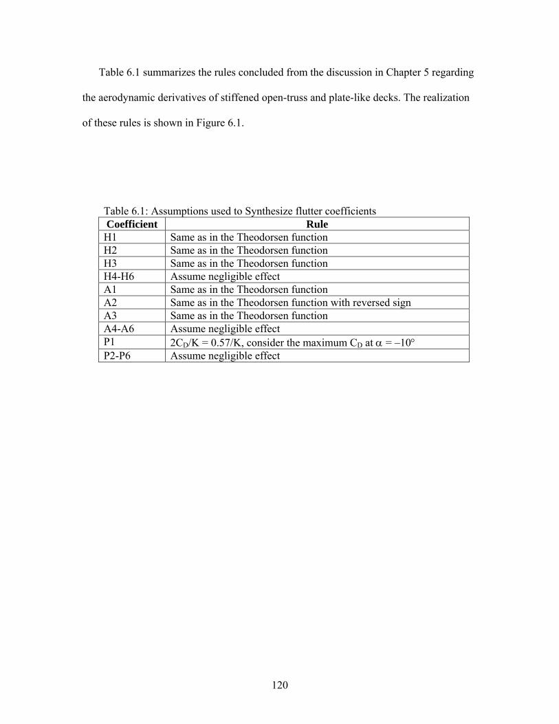
Table 6.1 summarizes the rules concluded from the discussion in Chapter 5 regarding

the aerodynamic derivatives of stiffened open-truss and plate-like decks. The realization

of these rules is shown in Figure 6.1.

Table 6.1: Assumptions used to Synthesize flutter coefficients Coefficient Rule H1 Same as in the Theodorsen function H2 Same as in the Theodorsen function H3 Same as in the Theodorsen function H4-H6 Assume negligible effect A1 Same as in the Theodorsen function A2 Same as in the Theodorsen function with reversed sign A3 Same as in the Theodorsen function A4-A6 Assume negligible effect P1 2CD/K = 0.57/K, consider the maximum CD at α = –10° P2-P6 Assume negligible effect

120

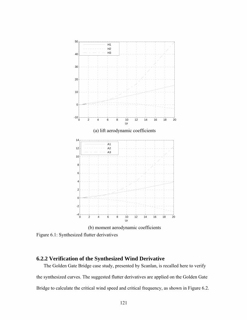
0 2 4 6 8 10 12 14 16 18 20-10

0

10

20

30

40

50

Ur

H1H2H3

(a) lift aerodynamic coefficients

0 2 4 6 8 10 12 14 16 18 20-4

-2

0

2

4

6

8

10

12

14

Ur

A1A2A3

(b) moment aerodynamic coefficients

Figure 6.1: Synthesized flutter derivatives

6.2.2 Verification of the Synthesized Wind Derivative The Golden Gate Bridge case study, presented by Scanlan, is recalled here to verify

the synthesized curves. The suggested flutter derivatives are applied on the Golden Gate

Bridge to calculate the critical wind speed and critical frequency, as shown in Figure 6.2.

121

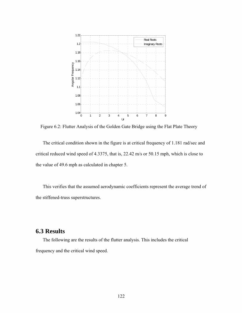
0 1 2 3 4 5 6 7 8 91.04

1.06

1.08

1.1

1.12

1.14

1.16

1.18

1.2

1.22

Ur

Ang

ular

Fre

quen

cy

Real RootsImaginary Roots

Figure 6.2: Flutter Analysis of the Golden Gate Bridge using the Flat Plate Theory

The critical condition shown in the figure is at critical frequency of 1.181 rad/sec and

critical reduced wind speed of 4.3375, that is, 22.42 m/s or 50.15 mph, which is close to

the value of 49.6 mph as calculated in chapter 5.

This verifies that the assumed aerodynamic coefficients represent the average trend of

the stiffened-truss superstructures.

6.3 Results The following are the results of the flutter analysis. This includes the critical

frequency and the critical wind speed.

122

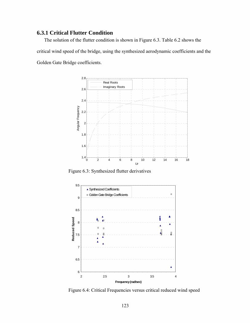
6.3.1 Critical Flutter Condition The solution of the flutter condition is shown in Figure 6.3. Table 6.2 shows the

critical wind speed of the bridge, using the synthesized aerodynamic coefficients and the

Golden Gate Bridge coefficients.

0 2 4 6 8 10 12 14 16 181.4

1.6

1.8

2

2.2

2.4

2.6

2.8

Ur

Ang

ular

Fre

quen

cyReal RootsImaginary Roots

Figure 6.3: Synthesized flutter derivatives

6

6.5

7

7.5

8

8.5

9

9.5

2 2.5 3 3.5 4

Frequency (rad/sec)

Red

uced

Spe

ed

Synthesized Coefficients

Golden Gate Bridge Coefficients

Figure 6.4: Critical Frequencies versus critical reduced wind speed

123

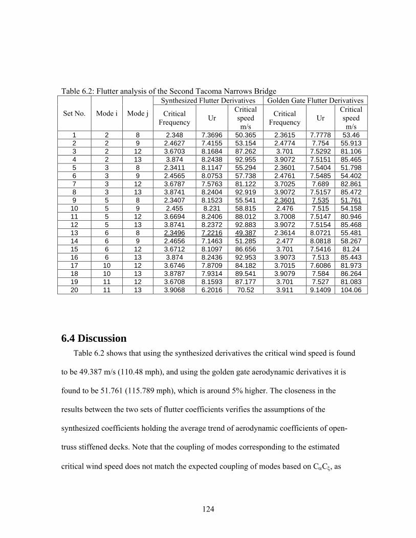
Table 6.2: Flutter analysis of the Second Tacoma Narrows Bridge

Synthesized Flutter Derivatives Golden Gate Flutter Derivatives

Set No. Mode i Mode j Critical Frequency Ur

Critical speed m/s

Critical Frequency Ur

Critical speed m/s

1 2 8 2.348 7.3696 50.365 2.3615 7.7778 53.46 2 2 9 2.4627 7.4155 53.154 2.4774 7.754 55.913 3 2 12 3.6703 8.1684 87.262 3.701 7.5292 81.106 4 2 13 3.874 8.2438 92.955 3.9072 7.5151 85.465 5 3 8 2.3411 8.1147 55.294 2.3601 7.5404 51.798 6 3 9 2.4565 8.0753 57.738 2.4761 7.5485 54.402 7 3 12 3.6787 7.5763 81.122 3.7025 7.689 82.861 8 3 13 3.8741 8.2404 92.919 3.9072 7.5157 85.472 9 5 8 2.3407 8.1523 55.541 2.3601 7.535 51.761 10 5 9 2.455 8.231 58.815 2.476 7.515 54.158 11 5 12 3.6694 8.2406 88.012 3.7008 7.5147 80.946 12 5 13 3.8741 8.2372 92.883 3.9072 7.5154 85.468 13 6 8 2.3496 7.2216 49.387 2.3614 8.0721 55.481 14 6 9 2.4656 7.1463 51.285 2.477 8.0818 58.267 15 6 12 3.6712 8.1097 86.656 3.701 7.5416 81.24 16 6 13 3.874 8.2436 92.953 3.9073 7.513 85.443 17 10 12 3.6746 7.8709 84.182 3.7015 7.6086 81.973 18 10 13 3.8787 7.9314 89.541 3.9079 7.584 86.264 19 11 12 3.6708 8.1593 87.177 3.701 7.527 81.083 20 11 13 3.9068 6.2016 70.52 3.911 9.1409 104.06

6.4 Discussion

Table 6.2 shows that using the synthesized derivatives the critical wind speed is found

to be 49.387 m/s (110.48 mph), and using the golden gate aerodynamic derivatives it is

found to be 51.761 (115.789 mph), which is around 5% higher. The closeness in the

results between the two sets of flutter coefficients verifies the assumptions of the

synthesized coefficients holding the average trend of aerodynamic coefficients of open-

truss stiffened decks. Note that the coupling of modes corresponding to the estimated

critical wind speed does not match the expected coupling of modes based on CαCξ, as

124

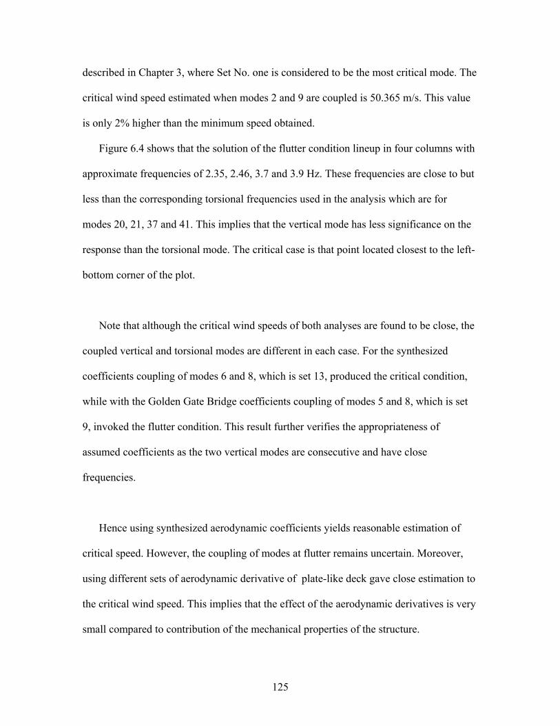
described in Chapter 3, where Set No. one is considered to be the most critical mode. The

critical wind speed estimated when modes 2 and 9 are coupled is 50.365 m/s. This value

is only 2% higher than the minimum speed obtained.

Figure 6.4 shows that the solution of the flutter condition lineup in four columns with

approximate frequencies of 2.35, 2.46, 3.7 and 3.9 Hz. These frequencies are close to but

less than the corresponding torsional frequencies used in the analysis which are for

modes 20, 21, 37 and 41. This implies that the vertical mode has less significance on the

response than the torsional mode. The critical case is that point located closest to the left-

bottom corner of the plot.

Note that although the critical wind speeds of both analyses are found to be close, the

coupled vertical and torsional modes are different in each case. For the synthesized

coefficients coupling of modes 6 and 8, which is set 13, produced the critical condition,

while with the Golden Gate Bridge coefficients coupling of modes 5 and 8, which is set

9, invoked the flutter condition. This result further verifies the appropriateness of

assumed coefficients as the two vertical modes are consecutive and have close

frequencies.

Hence using synthesized aerodynamic coefficients yields reasonable estimation of

critical speed. However, the coupling of modes at flutter remains uncertain. Moreover,

using different sets of aerodynamic derivative of plate-like deck gave close estimation to

the critical wind speed. This implies that the effect of the aerodynamic derivatives is very

small compared to contribution of the mechanical properties of the structure.

125

The maximum wind speed estimated in the Tacoma Narrows area is 105.9 mph, as

discussed in Chapter 4 as compared to 110.48 estimated here. Therefore according to this

analysis the bridge is safe, since the estimated flutter speed is around 4% higher than the

maximum expected wind speed.

126

CHAPTER 7 CONCLUSIONS AND RECOMMENDATIONS

The Second Tacoma Narrows Bridge frequencies have been successfully and

accurately estimated. The analytical results show sound agreement with the experimental

data. The transverse and the vertical frequencies are almost equal to the values obtained

by the ambient testing. However longitudinal frequencies do not show an accurate

agreement with the experimental results. The results are close to the experimental

frequencies.

The suggested modelling technique helped in concluding such results. Modelling

of suspension bridges requires using centenary element formulation. A non-linear truss

element is not quite acceptable to model cables. Detailed modelling of the superstructure

is also recommended. Moreover, the Ritz method was very successful in estimating the

structural frequencies and eliminating the local mode shapes.

The frequencies associated with the longitudinal mode shapes, however, do not

show high accuracy compared with the ambient study. However, this does not have a

significant effect on the aerodynamic analysis; that is because of the fact that the

longitudinal frequencies will not be excited by wind forces. Moreover, the torsional and

the vertical modes are not coupled with the longitudinal mode.

Flutter coefficients of open-truss stiffened superstructures are successfully

synthesized based on the Theodorsen function. It is found that reversing the sign of the

127

torsional aerodynamic damping coefficient of the flat plate simulates the average value of

this type of superstructures. This conclusion is not applicable for streamlined decks or

superstructures susceptible to vortex induced motion, such as, H-shape decks.

Recommendations According to the proposed procedure of synthesizing the flutter derivatives and

the methods used to find the critical wind speed of stiffened truss decks closing the open-

grates of the Second Tacoma Narrows Bridge will not cause the bridge to reach the

critical flutter condition. However, keeping the side grates opened ensures the safety of

the bridge in severe wind conditions, Matsumoto et al (2001).

The research on using computational-fluid-dynamics and fluid-structure-

interaction procedures in the flutter analysis of long-span bridges is still a novel field of

study. Some computational-fluid-dynamics software packages and numerical procedures

are still under development and investigation. The reliability of obtaining a valid solution

depends mainly on the capabilities of the used software. The solution of the FSI problem

may exhibit rational response, but may also involve inaccurate numerical values. For a

more reliable analysis, it is recommend utilizing powerful computational resources with

multi-processing capabilities and three-dimensional models, rather than a simplified two

dimensional characterization. Future research may also consider applying turbulence

models to account for the variable component of flow velocity

128

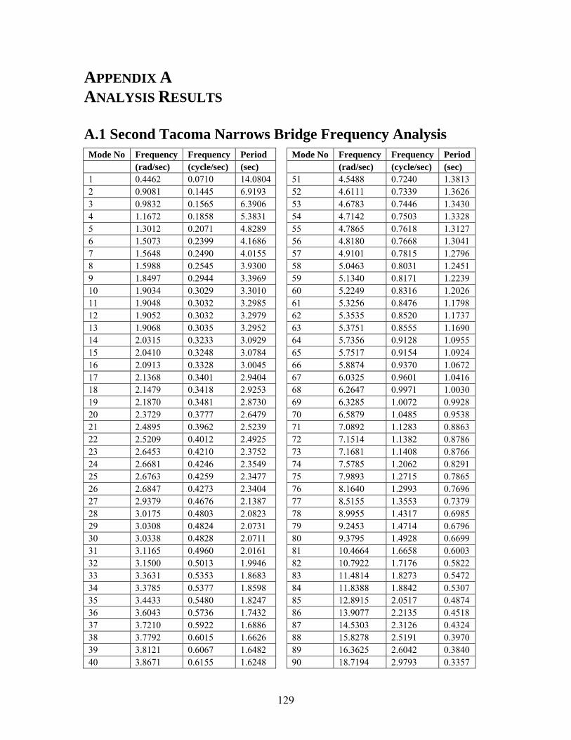
APPENDIX A ANALYSIS RESULTS A.1 Second Tacoma Narrows Bridge Frequency Analysis Mode No Frequency Frequency Period Mode No Frequency Frequency Period (rad/sec) (cycle/sec) (sec) (rad/sec) (cycle/sec) (sec) 1 0.4462 0.0710 14.0804 51 4.5488 0.7240 1.3813 2 0.9081 0.1445 6.9193 52 4.6111 0.7339 1.3626 3 0.9832 0.1565 6.3906 53 4.6783 0.7446 1.3430 4 1.1672 0.1858 5.3831 54 4.7142 0.7503 1.3328 5 1.3012 0.2071 4.8289 55 4.7865 0.7618 1.3127 6 1.5073 0.2399 4.1686 56 4.8180 0.7668 1.3041 7 1.5648 0.2490 4.0155 57 4.9101 0.7815 1.2796 8 1.5988 0.2545 3.9300 58 5.0463 0.8031 1.2451 9 1.8497 0.2944 3.3969 59 5.1340 0.8171 1.2239 10 1.9034 0.3029 3.3010 60 5.2249 0.8316 1.2026 11 1.9048 0.3032 3.2985 61 5.3256 0.8476 1.1798 12 1.9052 0.3032 3.2979 62 5.3535 0.8520 1.1737 13 1.9068 0.3035 3.2952 63 5.3751 0.8555 1.1690 14 2.0315 0.3233 3.0929 64 5.7356 0.9128 1.0955 15 2.0410 0.3248 3.0784 65 5.7517 0.9154 1.0924 16 2.0913 0.3328 3.0045 66 5.8874 0.9370 1.0672 17 2.1368 0.3401 2.9404 67 6.0325 0.9601 1.0416 18 2.1479 0.3418 2.9253 68 6.2647 0.9971 1.0030 19 2.1870 0.3481 2.8730 69 6.3285 1.0072 0.9928 20 2.3729 0.3777 2.6479 70 6.5879 1.0485 0.9538 21 2.4895 0.3962 2.5239 71 7.0892 1.1283 0.8863 22 2.5209 0.4012 2.4925 72 7.1514 1.1382 0.8786 23 2.6453 0.4210 2.3752 73 7.1681 1.1408 0.8766 24 2.6681 0.4246 2.3549 74 7.5785 1.2062 0.8291 25 2.6763 0.4259 2.3477 75 7.9893 1.2715 0.7865 26 2.6847 0.4273 2.3404 76 8.1640 1.2993 0.7696 27 2.9379 0.4676 2.1387 77 8.5155 1.3553 0.7379 28 3.0175 0.4803 2.0823 78 8.9955 1.4317 0.6985 29 3.0308 0.4824 2.0731 79 9.2453 1.4714 0.6796 30 3.0338 0.4828 2.0711 80 9.3795 1.4928 0.6699 31 3.1165 0.4960 2.0161 81 10.4664 1.6658 0.6003 32 3.1500 0.5013 1.9946 82 10.7922 1.7176 0.5822 33 3.3631 0.5353 1.8683 83 11.4814 1.8273 0.5472 34 3.3785 0.5377 1.8598 84 11.8388 1.8842 0.5307 35 3.4433 0.5480 1.8247 85 12.8915 2.0517 0.4874 36 3.6043 0.5736 1.7432 86 13.9077 2.2135 0.4518 37 3.7210 0.5922 1.6886 87 14.5303 2.3126 0.4324 38 3.7792 0.6015 1.6626 88 15.8278 2.5191 0.3970 39 3.8121 0.6067 1.6482 89 16.3625 2.6042 0.3840 40 3.8671 0.6155 1.6248 90 18.7194 2.9793 0.3357

129

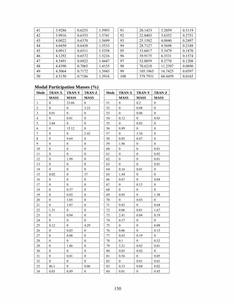
41 3.9286 0.6253 1.5993 91 20.1433 3.2059 0.3119 42 3.9916 0.6353 1.5741 92 22.8403 3.6352 0.2751 43 4.0022 0.6370 1.5699 93 25.1582 4.0040 0.2497 44 4.0450 0.6438 1.5533 94 28.7127 4.5698 0.2188 45 4.0913 0.6511 1.5358 95 33.6017 5.3479 0.1870 46 4.1292 0.6572 1.5216 96 39.9175 6.3531 0.1574 47 4.3491 0.6922 1.4447 97 52.0059 8.2770 0.1208 48 4.4390 0.7065 1.4155 98 70.6210 11.2397 0.0890 49 4.5064 0.7172 1.3943 99 105.1965 16.7425 0.0597 50 4.5150 0.7186 1.3916 100 379.7931 60.4459 0.0165

Modal Participation Masses (%)

Mode TRAN-X TRAN-Y TRAN-Z Mode TRAN-X TRAN-Y TRAN-Z MASS MASS MASS MASS MASS MASS 1 0 23.68 0 51 0 0.2 0 2 0 0 3.23 52 0 0.08 0 3 0.01 0 0 53 0 0.06 0 4 0 0.01 0 54 0.12 0 0.03 5 3.04 0 0 55 0 0.03 0 6 0 15.12 0 56 0.89 0 0 7 0 0 2.42 57 0 3.34 0 8 0 9.64 0 58 0.05 0.67 0 9 0 0 0 59 1.96 0 0 10 0 0 0 60 0 0 0.01 11 0 0 0 61 0 0 0.02 12 0 1.99 0 62 0 0 0.01 13 0 0 0 63 0 0 0.01 14 0 0 0 64 0.16 0.01 0 15 0.02 0 37 65 1.44 0 0 16 0 0 0 66 0.67 0 0.04 17 0 0 0 67 0 0.13 0 18 0 0.37 0 68 0 0 0 19 0 0.03 0 69 0.05 0 1.38 20 0 3.05 0 70 0 0.03 0 21 0 3.07 0 71 0.83 0 0.68 22 1.31 0 0 72 0.06 0.01 1.67 23 0 0.04 0 73 2.41 0.04 0.19 24 0 0 0 74 0.37 0 0 25 0.12 0 4.29 75 0 0 0.08 26 0 0.03 0 76 0.06 0 0.15 27 0 0.08 0 77 0.65 0.19 0 28 0 0 0 78 0.1 0 0.52 29 0 1.86 0 79 3.21 0.02 0.01 30 0 0 0 80 0.05 0.02 0 31 0 0.01 0 81 0.56 0 0.05 32 0 0 0 82 0 0.01 0.01 33 46.1 0 0.06 83 0.33 0.04 0.02 34 0.03 0.89 0 84 0.01 0 0.45

130

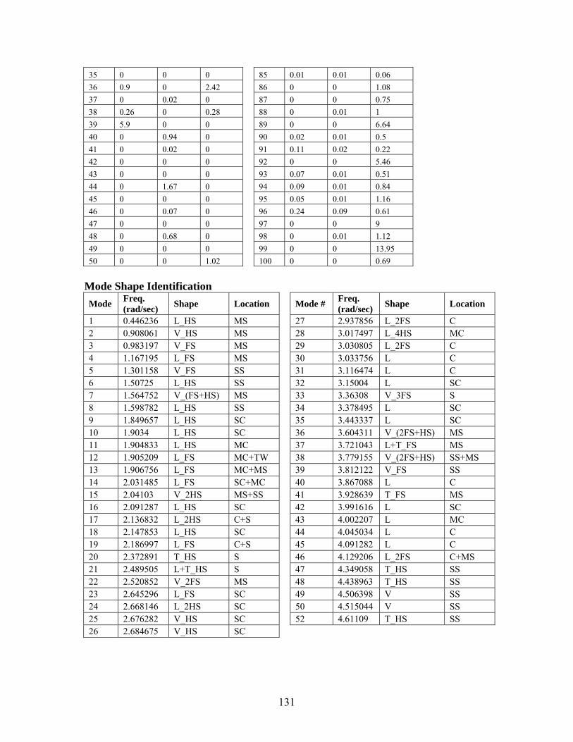
35 0 0 0 85 0.01 0.01 0.06 36 0.9 0 2.42 86 0 0 1.08 37 0 0.02 0 87 0 0 0.75 38 0.26 0 0.28 88 0 0.01 1 39 5.9 0 0 89 0 0 6.64 40 0 0.94 0 90 0.02 0.01 0.5 41 0 0.02 0 91 0.11 0.02 0.22 42 0 0 0 92 0 0 5.46 43 0 0 0 93 0.07 0.01 0.51 44 0 1.67 0 94 0.09 0.01 0.84 45 0 0 0 95 0.05 0.01 1.16 46 0 0.07 0 96 0.24 0.09 0.61 47 0 0 0 97 0 0 9 48 0 0.68 0 98 0 0.01 1.12 49 0 0 0 99 0 0 13.95 50 0 0 1.02 100 0 0 0.69

Mode Shape Identification Mode Freq.

(rad/sec) Shape Location Mode # Freq. (rad/sec) Shape Location

1 0.446236 L_HS MS 27 2.937856 L_2FS C 2 0.908061 V_HS MS 28 3.017497 L_4HS MC 3 0.983197 V_FS MS 29 3.030805 L_2FS C 4 1.167195 L_FS MS 30 3.033756 L C 5 1.301158 V_FS SS 31 3.116474 L C 6 1.50725 L_HS SS 32 3.15004 L SC 7 1.564752 V_(FS+HS) MS 33 3.36308 V_3FS S 8 1.598782 L_HS SS 34 3.378495 L SC 9 1.849657 L_HS SC 35 3.443337 L SC 10 1.9034 L_HS SC 36 3.604311 V_(2FS+HS) MS 11 1.904833 L_HS MC 37 3.721043 L+T_FS MS 12 1.905209 L_FS MC+TW 38 3.779155 V_(2FS+HS) SS+MS 13 1.906756 L_FS MC+MS 39 3.812122 V_FS SS 14 2.031485 L_FS SC+MC 40 3.867088 L C 15 2.04103 V_2HS MS+SS 41 3.928639 T_FS MS 16 2.091287 L_HS SC 42 3.991616 L SC 17 2.136832 L_2HS C+S 43 4.002207 L MC 18 2.147853 L_HS SC 44 4.045034 L C 19 2.186997 L_FS C+S 45 4.091282 L C 20 2.372891 T_HS S 46 4.129206 L_2FS C+MS 21 2.489505 L+T_HS S 47 4.349058 T_HS SS 22 2.520852 V_2FS MS 48 4.438963 T_HS SS 23 2.645296 L_FS SC 49 4.506398 V SS 24 2.668146 L_2HS SC 50 4.515044 V SS 25 2.676282 V_HS SC 52 4.61109 T_HS SS 26 2.684675 V_HS SC

131

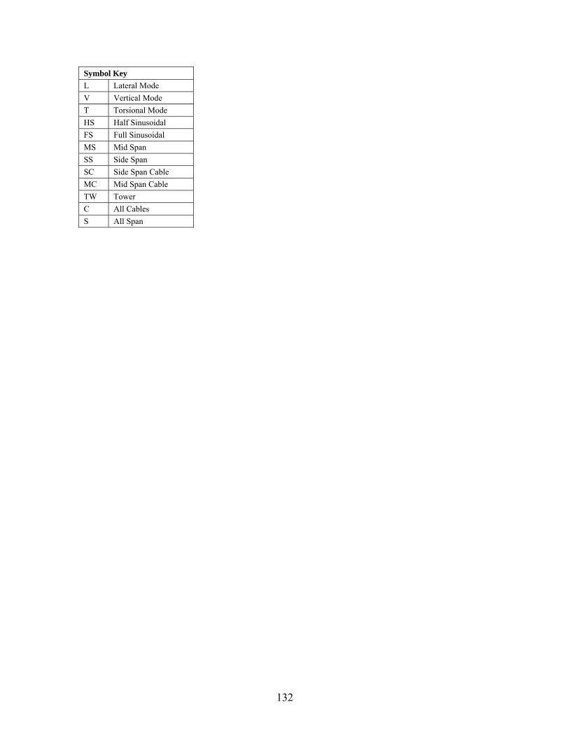
Symbol Key L Lateral Mode V Vertical Mode T Torsional Mode HS Half Sinusoidal FS Full Sinusoidal MS Mid Span SS Side Span SC Side Span Cable MC Mid Span Cable TW Tower C All Cables S All Span

132

APPENDIX B MATLAB PROGRAMS B.1 Coupling Coefficient %FindGenProp % Find the Generelized Properties and Coupling Terms mMat=[2 8;3 8;5 8;6 8; 2 9;3 9;5 9;6 9; 10 12;11 12;10 13;11 13] for m=1:12 mod1=mMat(m,1); mod2=mMat(m,2); [nr,nc]=size(Modeshp); Cx12=0;Cx11=0;Cx22=0; for i=1:nr-1; Cx1=(Modeshp(i,modXi+1)+Modeshp(i+1,modXi+1))/2; Cx2=(Modeshp(i,modA+1)+Modeshp(i+1,modA+1))/2; Cx12=Cx12+Cx1*Cx2*Modeshp(i,1); Cx11=Cx11+Cx1*Cx1*Modeshp(i,1); Cx22=Cx22+Cx2*Cx2*Modeshp(i,1); end CXi=abs(Cx12/Cx11); CA=abs(Cx12/Cx22); CouplingResult(m,:)=[mod1,mod2,CXi,CA] end

B.2 Flutter Analysis MATLAB Program % Uncoupled Flutter Solver clear clc stp=0; %ModesDataBase_FlatPlate % Xi index is for heaving, A index is for Rotation BrdgWidth=27.5; %meter AirDensity=1.2; OmegaXi=0.1285*2*pi; OmegaXi=0.1638*2*pi; OmegaA=0.1916*2*pi; ZetaA=0.005; % Damping ratio ZetaXi=0.005; CXi=.34; CA=.32; EffMassXi=5.2081e+003;

133

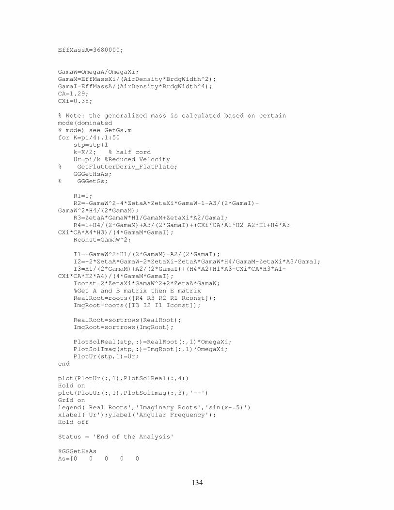
EffMassA=3680000; GamaW=OmegaA/OmegaXi; GamaM=EffMassXi/(AirDensity*BrdgWidth^2); GamaI=EffMassA/(AirDensity*BrdgWidth^4); CA=1.29; CXi=0.38; % Note: the generalized mass is calculated based on certain mode(dominated % mode) see GetGs.m for K=pi/4:.1:50 stp=stp+1 k=K/2; % half cord Ur=pi/k %Reduced Velocity % GetFlutterDeriv_FlatPlate; GGGetHsAs; % GGGetGs; R1=0; R2=-GamaW^2-4*ZetaA*ZetaXi*GamaW-1-A3/(2*GamaI)-GamaW^2*H4/(2*GamaM); R3=ZetaA*GamaW*H1/GamaM+ZetaXi*A2/GamaI; R4=1+H4/(2*GamaM)+A3/(2*GamaI)+(CXi*CA*A1*H2-A2*H1+H4*A3-CXi*CA*A4*H3)/(4*GamaM*GamaI); Rconst=GamaW^2; I1=-GamaW^2*H1/(2*GamaM)-A2/(2*GamaI); I2=-2*ZetaA*GamaW-2*ZetaXi-ZetaA*GamaW*H4/GamaM-ZetaXi*A3/GamaI; I3=H1/(2*GamaM)+A2/(2*GamaI)+(H4*A2+H1*A3-CXi*CA*H3*A1-CXi*CA*H2*A4)/(4*GamaM*GamaI); Iconst=2*ZetaXi*GamaW^2+2*ZetaA*GamaW; %Get A and B matrix then E matrix RealRoot=roots([R4 R3 R2 R1 Rconst]); ImgRoot=roots([I3 I2 I1 Iconst]); RealRoot=sortrows(RealRoot); ImgRoot=sortrows(ImgRoot); PlotSolReal(stp,:)=RealRoot(:,1)*OmegaXi; PlotSolImag(stp,:)=ImgRoot(:,1)*OmegaXi; PlotUr(stp,1)=Ur; end plot(PlotUr(:,1),PlotSolReal(:,4)) Hold on plot(PlotUr(:,1),PlotSolImag(:,3),'--') Grid on legend('Real Roots','Imaginary Roots','sin(x-.5)') xlabel('Ur');ylabel('Angular Frequency'); Hold off Status = 'End of the Analysis' %GGGetHsAs As=[0 0 0 0 0

134

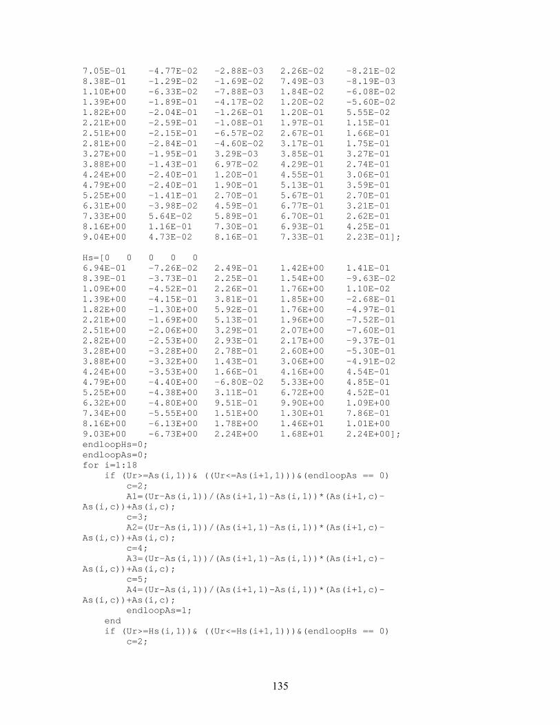
7.05E-01 -4.77E-02 -2.88E-03 2.26E-02 -8.21E-02 8.38E-01 -1.29E-02 -1.69E-02 7.49E-03 -8.19E-03 1.10E+00 -6.33E-02 -7.88E-03 1.84E-02 -6.08E-02 1.39E+00 -1.89E-01 -4.17E-02 1.20E-02 -5.60E-02 1.82E+00 -2.04E-01 -1.26E-01 1.20E-01 5.55E-02 2.21E+00 -2.59E-01 -1.08E-01 1.97E-01 1.15E-01 2.51E+00 -2.15E-01 -6.57E-02 2.67E-01 1.66E-01 2.81E+00 -2.84E-01 -4.60E-02 3.17E-01 1.75E-01 3.27E+00 -1.95E-01 3.29E-03 3.85E-01 3.27E-01 3.88E+00 -1.43E-01 6.97E-02 4.29E-01 2.74E-01 4.24E+00 -2.40E-01 1.20E-01 4.55E-01 3.06E-01 4.79E+00 -2.40E-01 1.90E-01 5.13E-01 3.59E-01 5.25E+00 -1.41E-01 2.70E-01 5.67E-01 2.70E-01 6.31E+00 -3.98E-02 4.59E-01 6.77E-01 3.21E-01 7.33E+00 5.64E-02 5.89E-01 6.70E-01 2.62E-01 8.16E+00 1.16E-01 7.30E-01 6.93E-01 4.25E-01 9.04E+00 4.73E-02 8.16E-01 7.33E-01 2.23E-01]; Hs=[0 0 0 0 0 6.94E-01 -7.26E-02 2.49E-01 1.42E+00 1.41E-01 8.39E-01 -3.73E-01 2.25E-01 1.54E+00 -9.63E-02 1.09E+00 -4.52E-01 2.26E-01 1.76E+00 1.10E-02 1.39E+00 -4.15E-01 3.81E-01 1.85E+00 -2.68E-01 1.82E+00 -1.30E+00 5.92E-01 1.76E+00 -4.97E-01 2.21E+00 -1.69E+00 5.13E-01 1.96E+00 -7.52E-01 2.51E+00 -2.06E+00 3.29E-01 2.07E+00 -7.60E-01 2.82E+00 -2.53E+00 2.93E-01 2.17E+00 -9.37E-01 3.28E+00 -3.28E+00 2.78E-01 2.60E+00 -5.30E-01 3.88E+00 -3.32E+00 1.43E-01 3.06E+00 -4.91E-02 4.24E+00 -3.53E+00 1.66E-01 4.16E+00 4.54E-01 4.79E+00 -4.40E+00 -6.80E-02 5.33E+00 4.85E-01 5.25E+00 -4.38E+00 3.11E-01 6.72E+00 4.52E-01 6.32E+00 -4.80E+00 9.51E-01 9.90E+00 1.09E+00 7.34E+00 -5.55E+00 1.51E+00 1.30E+01 7.86E-01 8.16E+00 -6.13E+00 1.78E+00 1.46E+01 1.01E+00 9.03E+00 -6.73E+00 2.24E+00 1.68E+01 2.24E+00]; endloopHs=0; endloopAs=0; for i=1:18 if (Ur>=As(i,1))& ((Ur<=As(i+1,1)))&(endloopAs == 0) c=2; A1=(Ur-As(i,1))/(As(i+1,1)-As(i,1))*(As(i+1,c)-As(i,c))+As(i,c); c=3; A2=(Ur-As(i,1))/(As(i+1,1)-As(i,1))*(As(i+1,c)-As(i,c))+As(i,c); c=4; A3=(Ur-As(i,1))/(As(i+1,1)-As(i,1))*(As(i+1,c)-As(i,c))+As(i,c); c=5; A4=(Ur-As(i,1))/(As(i+1,1)-As(i,1))*(As(i+1,c)-As(i,c))+As(i,c); endloopAs=1; end if (Ur>=Hs(i,1))& ((Ur<=Hs(i+1,1)))&(endloopHs == 0) c=2;

135

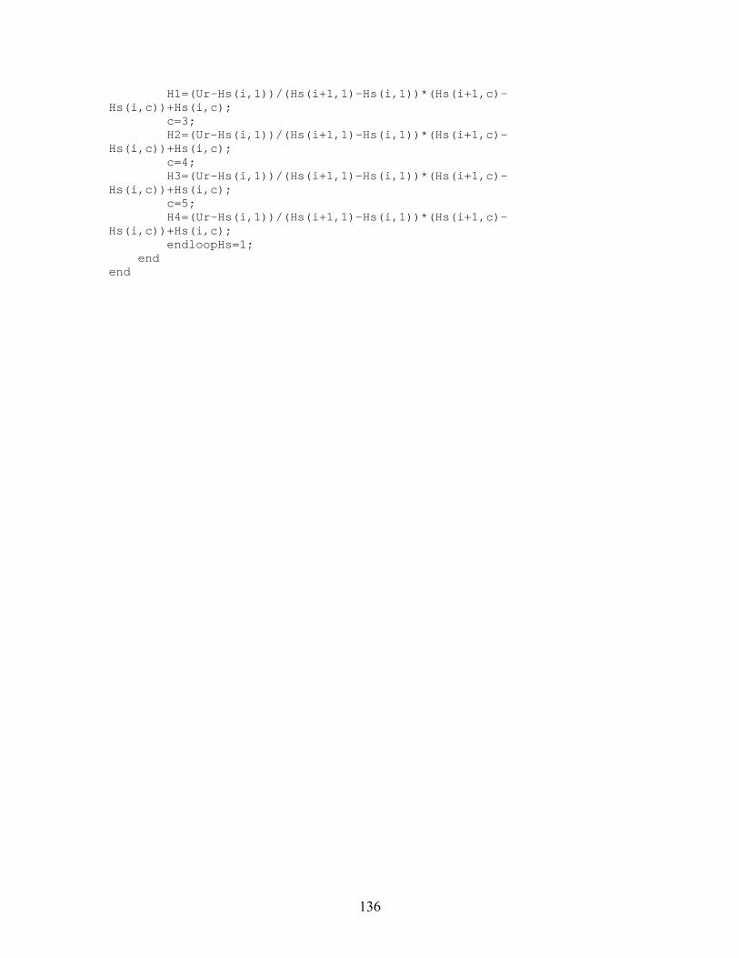
H1=(Ur-Hs(i,1))/(Hs(i+1,1)-Hs(i,1))*(Hs(i+1,c)-Hs(i,c))+Hs(i,c); c=3; H2=(Ur-Hs(i,1))/(Hs(i+1,1)-Hs(i,1))*(Hs(i+1,c)-Hs(i,c))+Hs(i,c); c=4; H3=(Ur-Hs(i,1))/(Hs(i+1,1)-Hs(i,1))*(Hs(i+1,c)-Hs(i,c))+Hs(i,c); c=5; H4=(Ur-Hs(i,1))/(Hs(i+1,1)-Hs(i,1))*(Hs(i+1,c)-Hs(i,c))+Hs(i,c); endloopHs=1; end end

136

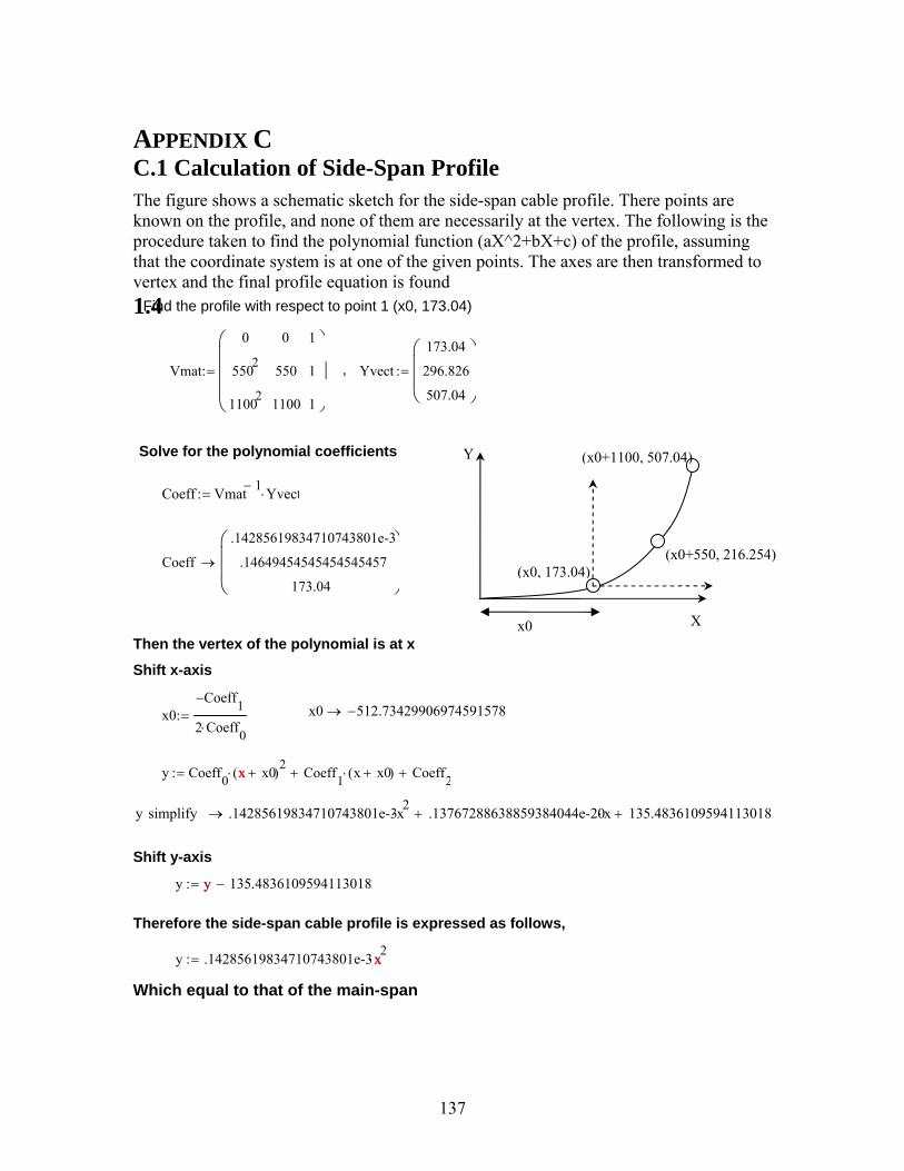
APPENDIX C C.1 Calculation of Side-Span Profile The figure shows a schematic sketch for the side-span cable profile. There points are known on the profile, and none of them are necessarily at the vertex. The following is the procedure taken to find the polynomial function (aX^2+bX+c) of the profile, assuming that the coordinate system is at one of the given points. The axes are then transformed to vertex and the final profile equation is found 1.4 Find the profile with respect to point 1 (x0, 173.04)

Vmat

0

5502

11002

0

550

1100

1

1

1

⎛⎜⎜⎜⎝

⎞

⎟

⎠

:= Yvect

173.04

296.826

507.04

⎛⎜⎜⎝

⎞

⎠:= ,

Solve for the polynomial coefficients Y

Coeff Vmat 1− Yvect⋅:=

Coeff

.14285619834710743801e-3

.14649454545454545457

173.04

⎛⎜⎜⎝

⎞

⎠→ (x0+550, 216.254)

(x0, 173.04)

(x0+1100, 507.04)

X x0Then the vertex of the polynomial is at x

Shift x-axis

x0Coeff1−

2 Coeff0⋅:= x0 512.73429906974591578−→

y Coeff0 x + x0( )2⋅ Coeff1 x x0+( )⋅+ Coeff2+:=

135.4836109594113018

x

y

y simplify .14285619834710743801e-3x2⋅ .13767288638859384044e-20x⋅+ 135.4836109594113018+→

Shift y-axis

y 8−:= y

x

Therefore the side-span cable profile is expressed as follows,

y .14285619834710743801e-3 2⋅:= x

Which equal to that of the main-span

137

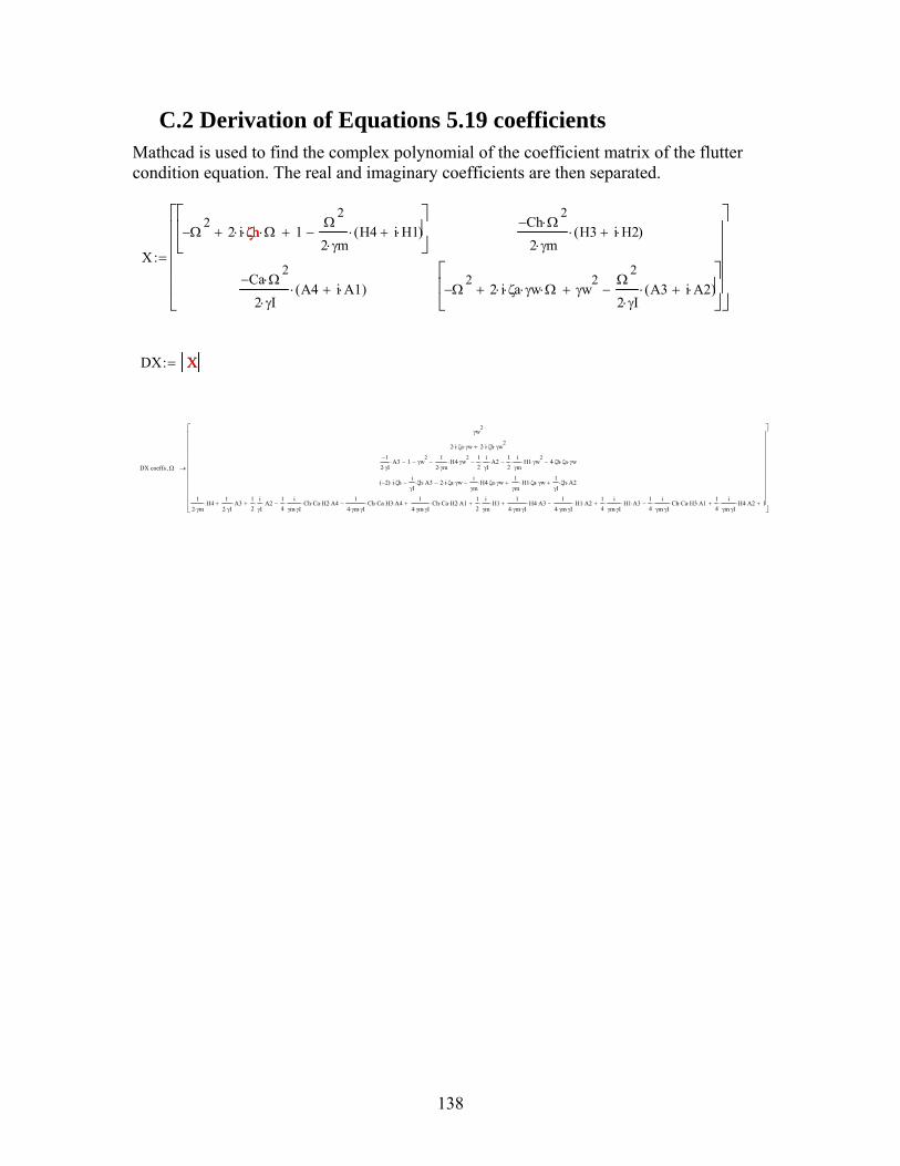
C.2 Derivation of Equations 5.19 coefficients Mathcad is used to find the complex polynomial of the coefficient matrix of the flutter condition equation. The real and imaginary coefficients are then separated.

X

Ω2

− 2 i⋅ ζh⋅ Ω⋅+ 1+Ω

2

2 γm⋅H4 i H1⋅+( )⋅−

⎡⎢⎣

⎤⎥⎦

Ca− Ω2

⋅

2 γI⋅A4 i A1⋅+( )⋅

Ch− Ω2

⋅

2 γm⋅H3 i H2⋅+( )⋅

Ω2

− 2 i⋅ ζa⋅ γw⋅ Ω⋅+ γw2

+Ω

2

2 γI⋅A3 i A2⋅+( )⋅−

⎡⎢⎣

⎤⎥⎦

⎡⎢⎢⎢⎢⎢⎣

⎤⎥⎥⎥⎥⎥⎦

:=

ζh

X

:=DX X

DX coeffs Ω,

γw2

2 i ζa γw⋅⋅⋅ 2 i ζh γw2

⋅⋅⋅+

1−2 γI⋅

A3⋅ 1− γw2

−1

2 γm⋅H4 γw

2⋅⋅−

12

iγI

A2⋅⋅−12

iγm

H1 γw2

⋅⋅⋅− 4 ζh ζa γw⋅⋅⋅−

2−( ) i ζh⋅⋅iγI

ζh A3⋅⋅− 2 i ζa γw⋅⋅⋅−iγm

H4 ζa γw⋅⋅⋅−1γm

H1 ζa γw⋅⋅⋅+1γI

ζh A2⋅⋅+

12 γm⋅

H4⋅1

2 γI⋅A3⋅+

12

iγI

A2⋅⋅14

iγm γI⋅

Ch Ca H2 A4⋅⋅⋅⋅⋅−1

4 γm γI⋅⋅Ch Ca H3 A4⋅⋅⋅⋅−+

14 γm γI⋅⋅

Ch Ca H2 A1⋅⋅⋅⋅+12

iγm

H1⋅⋅+1

4 γm γI⋅⋅H4 A3⋅⋅

14 γm γI⋅⋅

H1 A2⋅⋅−+14

iγm γI⋅

H1 A3⋅⋅⋅14

iγm γI⋅

Ch Ca H3 A1⋅⋅⋅⋅⋅−+14

iγm γI⋅

H4 A2⋅⋅⋅+ 1+

⎡⎢⎢⎢⎢⎢⎢⎢⎢⎢⎢⎣

⎤⎥⎥⎥⎥⎥⎥⎥⎥⎥⎥⎦

→

138

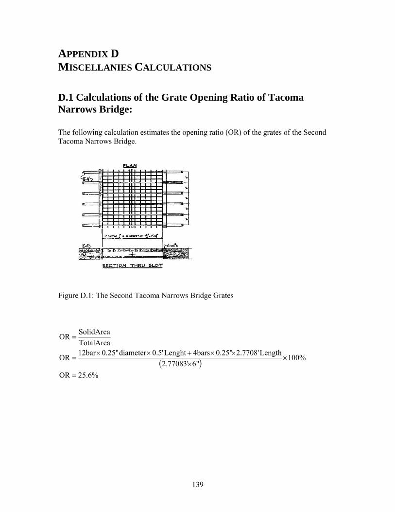
APPENDIX D MISCELLANIES CALCULATIONS

D.1 Calculations of the Grate Opening Ratio of Tacoma Narrows Bridge: The following calculation estimates the opening ratio (OR) of the grates of the Second Tacoma Narrows Bridge.

Figure D.1: The Second Tacoma Narrows Bridge Grates

( )25.6%OR

100%6"2.77083'

Length2.7708'0.25"4barsLenght0.5'diameter0.25"12barOR

TotalAreaSolidAreaOR

=

××

××+××=

=

139

APPENDIX E PARAMETERS FOR AEROELASTICITY E.1 Wind Characteristics

In aerodynamic analysis the wind parameters are calculated based on spatial

considerations. The environment surrounding the structure has considerable effects on the

atmospheric boundary layer. Wind flow becomes turbulent and nonlinear with space and

time. This is due to several factors, such as friction with the terrain, temperature

variations between the air at terrain level and that of higher altitudes, and the difference

in pressure from one zone to another.

Wind boundary layer is described by exponential profile of the mean wind speed and

a variable component of the turbulent speed. There is no clear formulation to simulate the

turbulent component of wind speed and stochastic method based on random functions

which are used to generate this component analytically.

For certain regions the average temperature, pressure and surface roughness are used

to generate the shape of the boundary layer. This is important for slender vertical

structures such as high-raised buildings and towers. In suspension bridges, however,

averaged values at the elevation of the superstructure are sufficiently acceptable to

calculated wind characteristics, unless wind effects on the main towers is required.

Averaged wind parameters are calculated in the following section. Most of these

parameters, such as viscosity and density of air, are required for the fluid-structure-

interaction finite element analysis. For the classical flutter analysis, density of air is the

140

only wind variable required, and the interaction between the structure and the laminar

wind flow is depicted by other coefficients determined experimentally, as described in

Chapter 6.

Another important wind parameter is the maximum averaged expected wind speed for

a given number year return period at the structure site. This value is extracted using

statistical methods, where the collected wind data is fitted to a cumulative density

function. The wind speed corresponding to a certain probability of occurrence is then can

be obtained.

The following is a brief discussion for the wind parameters and the methods used to

numerically evaluate them for a given the bridge.

E.1.1 Estimating Wind Parameters The number of air molecules in a micrometer is 2.5x1010 molecules, at sea level and

standard temperature. In other words, the mean free path between molecules is 6.6x10-8

meter. Therefore, wind within the atmospheric layer is considered continuum (Bertin,

2002). This allows the gross behavior of air motion to be described using macroscopic

properties, such as density, viscosity and temperature.

Generally speaking, fluid is described by the following variables, namely, density,

viscosity, specific heat at constant pressure, specific heat at constant volume, thermal

141

conductivity, rate of heat generated per unit volume, thermal expansion coefficient and

bulk modulus of elasticity. However, in incompressible flows, with inconsiderable heat

transfer, all the above mention parameters are ignored, except density and viscosity. Bulk

modulus of elasticity is assumed very large, and specific heat at constant volume is

assumed to be equal to the specific heat at constant pressure.

The mentioned variables could be constants, time-dependent, temperature-dependent,

deformation-dependent or a combination of these conditions. Although the constant

material model is the simplest, it is the most applicable in civil engineering problems.

Wind properties within few hundred feet above the ground could be considered constant.

According to the U.S. Standard Atmosphere, 1976, the change in air density, between the

ground surface and that at 2000 ft elevation above the ground level is less than 5% when

the change in viscosity is less than 3% and the change in pressure is less than 8%, see

Bertin J, 2002.

Air properties could be measured in several units based on the different unit systems.

However, in computational fluid dynamics standard units are used, due to its standard

definition. Temperature, in fluid mechanics, is usually measured in Kelvin (K), rather

than Celsius or Fahrenheit. Kelvin is more appropriate temperature unit than the others

since it is derived based on molecular motion. Air pressure is traditionally measured

using standard atmospheric pressure units, which is based on mercury column length.

However, in computational fluid dynamics it is more appropriate to use the force per unit

area unit. The standard atmospheric pressure at sea level is 1.101325x105 N/m2.

142

Density of air does not have a unique value. Air continuum changes with respect to

temperature and pressure. Therefore the mass per unit volume is a function of pressure

and temperature. The equation of state of thermally perfect gases could be used to

express the density of air as given by:

RTpρ =

E.1

Where p is the pressure (N/m2), R is the gas constant, which is equal to 287.05

N.m/kg.K in SI units, and T is the temperature in (K). Note that in fluid-structure-

interaction analysis, pressure around the solid body changes due the motion of the solid

body. However, the change in pressure between two points in the fluid flow is negligible

compared to the absolute pressure value. Bertin J., 2002, suggests that the assumption of

constant density is a valid approximation for velocities below 100 m/s (223 mph), which

is higher than the maximum possible wind speed on structures.

Viscosity is measured by coefficient of, µ, which is the ratio of the shear stress

developed by the flow to the transverse gradient of velocity. Viscosity represents the

transport of momentum in the direction of the velocity gradient. All fluids have viscosity,

but not all flows are viscous.

143

For temperatures less than 3000 K, the coefficient of viscosity of air is independent of

pressures (see Svehla 1962), and could be related to temperature only, using Sutherland’s

equation:

E.24.110

10458.15.1

6

+×= −

TTµ

where T is the temperature in Kelvin and µ is the coefficient of viscosity (kg/s.m).

The ratio of the viscosity to the density is defined as the kinematic viscosity, ν, which

is measured in square meter per second is given by:

E.3ρµν =

The thermal conductivity of air is frequently used in turbulent flow models. It could

be expressed in terms of temperature as flows:

E.4112

1076.45.1

4

+×= −

TTk

where k is in cal/m.s.K, and T is the temperature in Kelvin. The conductivity is also

computed in J/m.s.K, where1 cal is 4.187 J (Bertin, 2002).

Another property of air is the speed of sound, which reflects the disturbance of

infinitesimal proportions propagating through fluid at rest. Generally, the speed of sound,

a, is given:

144

E.5RTa γ=

where γ is the ratio of specific heats (Cp/Cv = 1.4 for perfect gas), R is the gas

constant and T is the temperature. Therefore for air the speed of sound (m/s) is

Ta 047.20= , where T is in Kelvin. For a standard temperature the speed of sound is

around (346.1 m/s). It is suggested that air flow could be considered incompressible if its

speed is less than 0.3 Mach (103 m/s or 230 mph), see Wanderley and Levi, 2002.

Wind properties, as shown in the above equations, are mainly a function of

temperature and pressure. These two variables are not deterministic and are considered

stochastic variables. However, ignoring the variability in wind properties is accepted in

this research, since the extreme values of wind speed are required and the critical flutter

condition is to be evaluated, rather then a reliability assessment. Moreover, the variation

in wind properties between 37 °F and 100 °F is around 20%. If the mean value of this

temperature interval is considered then the variation would be around ±10%. Therefore,

temperature and pressure will be assumed constants and air density and viscosity will be

estimated accordingly as deterministic value. The pressure and temperature are assumed

based on the average metrological measurements in the Tacoma area in months of

maximum wind speed.

The following table summarizes average values of air properties that will be used for

analysis in this research.

145

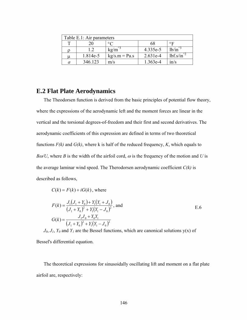
Table E.1: Air parameters

T 20 68 °C °F ρ 1.2 kg/m^3 4.335e-5 lb/in^3

lbf.s/in^2 1.814e-5 kg/s.m = Pa.s 2.631e-4 µ a 346.123 m/s 1.363e-4 in/s

E.2 Flat Plate Aerodynamics The Theodorsen function is derived from the basic principles of potential flow theory,

where the expressions of the aerodynamic left and the moment forces are linear in the

vertical and the torsional degrees-of-freedom and their first and second derivatives. The

aerodynamic coefficients of this expression are defined in terms of two theoretical

functions F(k) and G(k), where k is half of the reduced frequency, K, which equals to

Bω/U, where B is the width of the airfoil cord, ω is the frequency of the motion and U is

the average laminar wind speed. The Therodorsen aerodynamic coefficient C(k) is

described as follows,

)()()( kiGkFkC += , where

( ) (( ) (

))2011

201

011011)(JYYYJJYYYJJkF

−+++++

= , and E.6

( ) ( )20112

01

1001)(JYYYJ

YYJJkG−++

+=

J0, J1, Y0 and Y1 are the Bessel functions, which are canonical solutions y(x) of

Bessel's differential equation.

The theoretical expressions for sinusoidally oscillating lift and moment on a flat plate

airfoil are, respectively:

146

( ) ( )( )ααπραππαπρ &&&&&&& abhUkCbahUbLh −++−−+−= 212 )(2 E.7

( )( ) ( )( ) ( )( )ααπρ

παπαπρα

&&

&&&&&

abhUkCaUb

hbaabUbabM

−++++

−++−−=

21

212

2812

212

)(2 E.8

where, k and U are as defined above, ρ is the wind density, b is half of the length of

the airfoil cord (B), a is the distance from the mid-chord to the rotation point and h and α

are vertical and angular displacement, respectively. The dot and the double dots, appear

over α and h, are the first and second derivative with time, that is, velocity and

acceleration, respectively.

For bluff bodies, and suspension bridge decks, a different expression is suggested.

The expression is discussed in Chapter 6. In the expression of the aerodynamic forces of

bluff bodies, displacement and velocity terms of each degree-of-freedom are correlated to

separate aerodynamic coefficients. The above equations are equated to the aerodynamic

forces of suspension bridges, and an equivalent expression to the flat plate aerodynamic

forces, is obtained by evaluating the aerodynamic coefficients of the bluff body

correspondingly. These coefficients are expressed in Chapter 5.

147

REFERENCES

ADINA-F Manual (2006), ADINA R&D, Inc., Boston, USA

AGA and OPAC – Geospectra (1994), Tacoma Narrows Bridge Seismic

Vulnerability Study,

Ammann, O.H.; Karman, T. and Woodruff, G.B. (1941), The failure of the Tacoma

Narrows bridge, Report to the Federal Works Agency.

Barar, P. S.; Raul, R. and Scanlan, R. H. (1996), Numerical Calculation of Flutter

Derivatives Via Indicial Functions, Journal of Fluid and Structures, vol 10, pp. 337-

351

Barriga-Rivera, Alfredo Nicolas (1973), Aeroelastic Vibrations of Structural Shapes

in Highly Turbulent Flows, Master of Science thesis, Washington State University.

Bathe, K.J. and Zhang, H. (1999), Finite element analysis of fluid flows fully coupled

with structural interactions, Computers & Structures, Vol. 72, Issues 1-3, Pages 1-16

Bertin J. (2002), Aerodynamics for Engineering, Fourth Edition, Prentice Hall, New

Jersey,

Boussinesq, J. (1877), Théorie de l’écoulement Tourbillant, Mémoires Présentes par

Divers Savants de l’Académie des Science, Institut de France, Vol. 23, pp. 46-50

Brancaleoni, F. and Diana, G. (1993), The aerodynamic design of the Messina Straits

148

Bridge, Journal of Wind Engineering and Industrial Aerodynamics, Vol. 48 (2-3), p.

p 329-342

Brar, P. S.; Raul, R. and Scanlan, R. H. (1996), Numerical Calculation of Flutter

Derivative Via Indicial Function, Journal of Fluid and Structures, issue 10, p. 337 –

351

Cebeci, T. and Simth, A.M.O. (1974), Analysis of Turbulent Boundary Layers, Ser.

in Appl. Math and Mech., Vol. XV, Academic Press, Orlando, Florida

Cebeci, T. and Simth, A.M.O. (1974), Analysis of Turbulent Boundary Layers, Ser.

in Appl. Math and Mech., Vol. XV, Academic Press, Orlando, Florida

Chen W.F., Duan L. (1999), Bridge Engineering Handbook, CRC Press, Florida,

USA

Chopra, Anil (2001), Dynamics of Structures: Theory and Applications to

Earthquake Engineering, Third Edition, Pearson Education, Inc., New Jersey, USA.

Cigada, A.; Diana, G.; Falco, M.; Fossati, F. and Manenti, A. (1997), Vortex

shedding and wake-induced vibrations in single and bundle cables, Journal of Wind

Engineering and Industrial Aerodynamics, Vol. 72 , issue Nov.-Dec, Pages 253-263

Davenport, A. G. (1961), The Response of Slender, Line-like Structures to a Gusty

Wind, Proceedings of the Institute of Civil Engineering, 19, pp. 449-472

Diana, G.; Bruni, S.; Cigada, A. and Collina (1993), A., Turbulence Effect on Flutter

Velocity in Long Span Suspended Bridges, Journal of Wind Engineering and

149

Industrial Aerodynamics, Vol. 48 (2-3), p.p. 329-342

Dunn, L.G. (1941), The failure of the Tacoma Narrows bridge. Report to the Federal

Works Agency, Appendix VIII, Volume 28, issue March.

Dyrbye, C. and Hansen, S. (1997), Wind Loads on Structures, John Wiley and Sons,

England,

Farquharson, F. B. (1954), Aerodynamic Stability of Suspension Bridges: with special

reference to the Tacoma Narrows Bridge, The Structural Research Laboratory –

University of Washington, Seattle

Fiana, G.; Bruni, S.; Cigada, A. and Collina, A., Turbulence Effect on Flutter

Velocity in Long Span Suspended Bridges, Journal of Wind Engineering and

Industrial Aerodynamics, Vol. 48 (2-3) October 1993, p.p. 329-342

Frandsen J.B. (2004), Numerical bridge deck studies using finite elements. Part1:1

flutter, Journal of Fluid and Structures, 19, p. 171-191

Garrick, I.E. (1938), On some reciprocal relations in the theory of nonstationary

flows, NACA Tech. Report 629, Nat. Advisory Committee for Aeronautics, Langley,

VA.

Ge M.m Zhang R., Xiang H. (2000), Identification of flutter derivatives of bridge

decks, Journal of Engineering and Industrial Aerodynamics, volume 84, pp. 151-162

Ge Y.J. and Tanaka H. (2000), Aerodynamic flutter analysis of cable-supported

bridge by multi-mode and full-mode approaches, Journal of Wind Engineering and

150

Industrial Aerodynamics, vol. 86, p.: 123-153

Grant, I. and Barnes, F. H. (1981), The vortex shedding and drag associated with

structural elements, Journal of Wind Engineering and Industrial Aerodynamics,

Volume 8, Issues 1-2, Pages 115-122

Huston, D.; Bosch, H. and Scanlan, R. (1988), The Effects of Fairings and of

Turbulence on the Flutter Derivatives of a Notably Unstable Bridge Deck, Journal of

Wind Engineering and Industrial Aerodynamics, Vol. 29, p.p. 339-349.

Jones, N.P.; Scanlan, R.H.; Sarkar, P.P; Singh, L. (1995), The effect of Section Model

Details on Aeroelastic Parameters, Journal of Engineering and Industrial

Aerodynamics, Vol. 54/55, p.p. 45-53

Katsuchi H.; Jones N.P.; Scanlan R.H. (1998), Akiyama H., Multi-mode flutter and

buffeting analysis of the Akashi-Kaikyo bridge, Journal of Wind and Engineering and

Industrial Aerodynamics, vol. 77&78, p.: 431-441

Katsuchi, H.; Jones, N.P.; Scanlan, R.H.; Akiyama, H. (1998), Multi-mode flutter and

buffeting analysis of the Akashi-Kaikyo bridge, Journal of Wind Engineering and

Industrial Aerodynamics, Vol. 77&78, p.p. 431-441

Kussner, H.G. (1936), Zusammenfassender Bericht u ber den instation a ren Auftrieb

von Flugeln, Luftfahrt-Forschhung , 13, :410 - 424

Liepmann, H. W. (1952), On the Application of Statistical Concepts to the Buffeting

Problem, Journal of Aeronautical Science, 19, 12, pp. 793-822

151

Matsumoto, M.; Nakajima, N.; Taniwaki, Y.; Shijo, R. (2001), Grating effect on

flutter instability, Journal of Wind Engineering and Industrial Aerodynamics, Vol.

89, p.p. 1487-1497

O’Connor C (1971)., Design of Bridge Superstructures, Wiley-Interscience, New

York

OPAC Consulting Engineers (1993), Tacoma Narrows Bridge Seismic Vulnerability

Study: Calculations

Peterson, S. (2002), Experimental Response and Analysis of the Evergreen Point

Floating Bridge, A PhD dissertation, Washington State University

Prandtl, L. (1925), Uber die ausgebildete Turbulenz, ZAMM, Vol. 5, pp. 136-139

Prandtl, L. (1925), Uber die ausgebildete Turbulenz, ZAMM, Vol. 5, pp. 136-139

Prandtl, L. (1945), Uber ein neues Formelsystem fur die ausgebildete Turbulenz,

Nacr. Akad. Wiss. Gottingen, Math-Phys. Kl., pp. 6-19

Prandtl, L. (1945), Uber ein neues Formelsystem fur die ausgebildete Turbulenz,

Nacr. Akad. Wiss. Gottingen, Math-Phys. Kl. 1945, pp. 6-19

Pugsley, A., (1949), Some experimental work on model suspension bridges,

structural engineering, Volume 8, issue 27

Pugsley, Sr. Alfred (1968), The Theroy of Suspension Bridges, Second Edition,

Edward Arnold Publishers LTD, London, UK

152

Rotta, J. C. (1951), Statistische Theorie nichthomogener Turbulenz, Zeitschrift fur

Physik, Vol. 129, pp. 547-572

Rotta, J. C. (1951), Statistische Theorie nichthomogener Turbulenz, Zeitschrift fur

Physik, Vol. 129, pp. 547-572

Rowan Williams Davies & Irwin Inc (2003), Final Report – Volume 1 of 2, Wind

Engineering Studies: Tacoma Narrows Bridge, Ontario, Canada

Sarkar, P. (1992), New-identification methods applied to the response of flxiable

bridges to wind, PhD thesis, The John Hopkins University, Baltimore, Md.

Sarkar, P.P.; Jones, N.P. and Scanlan, R.H. (1994), Identification of aeroelastic

parameters of flexbale bridges, Journal of Engineering mechanics. ASCE 120,

p.p.1718-1742

Sarkar, Partha (1986), Effect of Wind Turbulence on The Stability of Long Span

Bridges, Master of Science Thesis, Washington State University, USA

Scanlan, R. (1988), On Flutter and Buffeting Mechanisms in Long-Span Bridges,

Journal of Probabilistic Engineering Mechanics, Vol. 3, No. 1, p.p. 22-27

Scanlan, R. H. (1983), On Linearized airfoil and bluff-body stability theory and the

scruton number, Journal of wind engineering and industrial aerodynamics, vol. 12,

pp. 373-378

Scanlan, R. H. and Tomko, J. J. (1971), Airfoil and bridge deck flutter derivatives,

Journal of the Engineering Mechanics Division, Proceedings pf the ASCE, Vol. 97,

153

No. EM 6, p.p. 1717-1737

Scanlan, R.H. and Budlong, K.S. (1972), Flutter and aerodynamic response

considerations for bluff objects in a smooth flow, Flow-induced structural vibrations,

Proc. Symp. IVTAM-IAHR, Karlsruhe, Springer, Berlin, Germany p.p339—354

Scanlan, R.H., and Sabzevari, A. (1967), Suspension bridge flutter revisited,

Proceedings of Structural Conference, ASCE, Paper No.468, New York

Scanlan, R.H.; and Rosenbaum, R. (1951), Aircraft Vibration and Flutter,

Macmillan, New York

Scanlan, R.H.; Jones, N.P.; Singh, L. (1997), Inter-relations among flutter

derivatives, Journal of Wind Engineering and Industrial Aerodynamics, Vol 69 – 71,

p.p. 829 – 837

Scnalan, R. and Lin, WH (1978), Effects of Turbulence on Bridge Flutter

Derivatives, Journal of the Engineering Mechanics Division, Proceedings of the

American Society of Civil Engineers, Vol. 104. No. 4

Sears, W.R. (1941), Some aspects of non-stationary airfoil theory and its practical

application, Journal of Aeronautical Science, Vol. 8, issue 3, p.p.104—108

Singh, L.; Jones, N.P.; Scanlan, R.H. and Lorendeaux, O. (1996), Identification of

lateral flutter derivatives of bridge decks, Journal of wind Engineering and Industrial

Aerodynamics, Vol. 60, p.p. 81-89

Svehla, R. A. (1962), Estimated Viscosities and Thermal conductivities of Gases at

154

High Temperatures, Technical Repot R-132 NASA

Svehla, R. A. (1962), Estimated Viscosities and Thermal conductivities of Gases at

High Temperatures, Technical Repot R-132 NASA

The ASCE 7-02 Committee (2003), Minimum Design Loads for Buildings and other

Structures: Revision of ASCE 7-98, ASCE Publication, Virginia, USA

Theodorsen T. (1935), General theory of aerodynamic instability and mechanism of

flutter, NACA Report 496, U.S. Nat. Advisory Committee for Aeronautics, Langley,

VA

Theodorsen, T. (1934), General theory of aerodynamic instability and the mechanism

of flutter, NACA a 496, National Aeronautics and space Administration

Ukeguchi, M.; Sakata, H. and Nishitani, H. (1966), An investigation of aeroelastic

instability of suspension bridges, Proceedings Symposium on Suspension Bridges,

Lisbon, Portugal

Wagner, H. (1925), U ber die Entstehung des dynamischen Auftriebs von

Tragflugein, Zeit. Angew. Math. U. Mech. 5(1) p.p.17—35

Wanderley, J.B. and Levi, C.A. (2002), Validation of a finite difference method for

the simulation of vortex-induced vibrations on a circular cylinder, Ocean

Engineering, 29, p.p. 445-460

Wanderley, J.B. and Levi, C.A. (2002), Validation of a finite difference method for

the simulation of vortex-induced vibrations on a circular cylinder, Ocean

155

Engineering, 29, p.p. 445-460

Wilcox D.C. (1993), Turbulence Modeling for CFD, DCW Industries, Inc.,

California

Wilcox, D.C. (1993), Turbulence Modeling for CFD, DCW Industries, Inc.,

California

Wilson E. (2002), Three Dimensional Static and Dynamic Analysis of Structures,

Computers and Structures Inc., Third Edition, Berkeley, CA, USA

Zhang H.; Zhang, Xiaoli; Ji, Shanhong; Guo, Yanhu; Ledezma, Gustavo; Elabbasi,

Nagi and deCougny, Hugues (2003), Recent development of fluid–structure

interaction capabilities in the ADINA system, Journal of Computers & Structures,

Volume 81, Issues 8-11, p.p. 1071-1085

Zhang, H. and Bathe, K.J. (2001), Direct and Iterative Computing of Fluid Flows

fully Coupled with Structures, Proceedings of the First MIT Conference on

Computational Fluid and Solid Mechanics, Boston, USA

156