Flutes vs. Cellos: Analyzing Mobility-TrafficCorrelations in Large WLAN Traces

Babak Alipour∗babak.ap@ufl.edu

Leonardo Tonetto†tonetto@in.tum.de

Aaron Yi Ding†ding@in.tum.de

Roozbeh Ketabi∗roozbeh@ufl.edu

Jörg Ott†ott@in.tum.de

Ahmed Helmy∗helmy@ufl.edu

∗Computer and Information Science and EngineeringUniversity of Florida, Gainesville, USA

†Department of InformaticsTechnical University of Munich, Munich, Germany

Abstract—Two major factors affecting mobile network per-formance are mobility and traffic patterns. Simulations andanalytical-based performance evaluations rely on models toapproximate factors affecting the network. Hence, the under-standing of mobility and traffic is imperative to the effec-tive evaluation and efficient design of future mobile networks.Current models target either mobility or traffic, but do notcapture their interplay. Many trace-based mobility models havelargely used pre-smartphone datasets (e.g., AP-logs), or muchcoarser granularity (e.g., cell-towers) traces. This raises questionsregarding the relevance of existing models, and motivates ourstudy to revisit this area. In this study, we conduct a multi-dimensional analysis, to quantitatively characterize mobility andtraffic spatio-temporal patterns, for laptops and smartphones,leading to a detailed integrated mobility-traffic analysis. Ourstudy is data-driven, as we collect and mine capacious datasets(with 30TB, 300k devices) that capture all of these dimensions.The investigation is performed using our systematic (FLAMeS)framework. Overall, dozens of mobility and traffic features havebeen analyzed. The insights and lessons learnt serve as guidelinesand a first step towards future integrated mobility-traffic models.In addition, our work acts as a stepping-stone towards a richer,more-realistic suite of mobile test scenarios and benchmarks.

I. INTRODUCTION

Human mobility has been studied extensively and manymodels have been derived. The spectrum ranges from simplesynthetic mobility models to complex trace-based models,capturing different properties with varying degrees of accuracy[1], [2]. Similarly, network traffic has been studied increas-ingly for wireless networks: for rather stationary users (as inWLANs) (e.g., [3], [4]) and potentially mobile users as forcellular networks (e.g., [5], [6]). Such analyses range frommetrics such as flow count, sizes, and traffic volume to serviceusage (e.g., visited web sites, backend services).

Both mobility and network usage, characterize differentaspects of human behavior. In this sense, we have a mobilityplane and a (network) traffic plane. In reality, these two planesare likely interdependent. Human mobility may be influencedby network activity; for example, a person slowing downto read incoming messages. Also, network activity may beinfluenced by mobility and location; stationary users mayproduce/consume more data than those walking, and peoplemay use different services in different places [7].

In earlier studies, this interdependence has not been widelyconsidered, and models for both mobility and network trafficplanes have been developed and evaluated largely in isolation.For example, when evaluating mobile systems’ performance,

traffic generation generally follows regular patterns, drawnfrom common simple distributions (e.g., exponential or uni-form), while assuming neither transmission nor reception ofdata impacts mobility. Simply observing people walking whilestaring at (or reacting to) their smartphones suggests, however,that such interdependencies need to be captured properly.Understanding the mobility-traffic interplay is imperative tothe effective evaluation and efficient design of future mobilealgorithms ranging from user behavior prediction and caching,to network load estimation and resource allocation.

In this paper, we take a stab at understanding the intercon-nection of the mobility and traffic planes. To do this properly,we need to consider the nature of mobile devices people use:one class of devices is merely intended for stationary use,typically while the user is seated—this primarily holds forlaptop computers, dubbed cellos. In contrast, another class—’on-the-go’ smartphones, which we refer to as flutes—lendthemselves to truly mobile use1. We focus our analysis onthese two classes because they have been around long enoughto have extensive datasets to build upon. We stipulate that theinterconnection of the mobility and traffic is modulated bythe device(s) a mobile user is carrying. Therefore, we followtwo main lines of investigation: we develop a framework todifferentiate between cellos and flutes, and study both themobility and traffic patterns for each of those types.

Specifically, the main goal of this paper is to quantitativelyinvestigate the following questions in-depth: (I) How differentare mobility and traffic characteristics across device types,time and space? (II) What are the relationships between thesecharacteristics? (III) Should new models be devised to capturethese differences? And, if so, how?

To answer these questions, a multi-dimensional (compara-tive) analysis approach is adopted to investigate mobility andtraffic spatio-temporal patterns for flutes and cellos. We driveour study with capacious datasets (30TB+) that capture all theabove dimensions in a campus society, including over 300kdevices (Sec. IV). A systematic Framework for Large-scaleAnalysis of Mobile Societies (FLAMeS) is devised for thisstudy, that can also be used to analyze other multi-sourceddata in future studies. Our main contributions include:

1) Integrated mobility-traffic analyses (Sec. VII): This studyis the first to quantify the correlations of numerous

1Throughout, we use flutes for smartphones, and cellos for laptops.

1

features of mobility and traffic simultaneously. This canidentify gaps in existing mobile networking models, andreopen the door for future impactful work in this area.

2) Flutes vs. Cellos analysis (Sec. V–VI): The device typeclassification presented here, is an important dimensionto understand. This is particularly relevant as new genera-tions of portable devices are introduced, that are differentthan laptops, traditionally considered in earlier studies.

3) Systematic multi-dimensional investigation framework(Sec. III): FLAMeS provides the scaffolding needed toprocess, in multiple dimensions, many features of largesets of measurements from wireless networks, includingAP-logs and NetFlow traces. This systematic method canapply to other datasets in future studies.

II. RELATED WORK

To characterize mobility and network usage, existing stud-ies have covered various aspects, including human mobility,device variation, and dataset analysis.

Human Mobility: Given its importance in various researchareas, human mobility has received significant attention. Werefer the reader to [1], [2] for surveys of mobility modelingand analysis. For spatial-temporal patterns, [8] and [9] revealthe regularity and bounds for predicting human mobility usingcellular logs. A recent study highlighted the importance ofcombining different datasets to study various features simul-taneously [10]. Our observations are similar to [8], [9], whichreaffirms the intrinsic properties of human mobility, despitedifferences in granularity and population across datasets. Toadvance the understanding of human mobility, we integrateddifferent datasets to correlate mobility and network traffic.

Device Variation: Usage and traffic patterns of differentdevice types have been studied from various perspectives([11], [12], [13], [14], [15], [16]). However, those findingsare based on classifications that rely on either MAC addressesor HTTP headers solely. The former is rather limited andthe latter may have serious privacy implications and areoften unavailable. In [17], authors use packet-level tracesfrom 10 phones and application-level monitoring from 33Android devices to analyze smartphone traffic. Although thisallowed fine-grained measurements, the approach is invasiveand limited in scalability, leading to small sample sizes andrestricted conclusions. They also do not compare the traffic ofsmartphones with that of “stop-to-use” wireless devices (i.e.cellos) nor do they measure spatial metrics. The study in [18]analyzes 32k users on campus, and focuses on multi-deviceusage. It notes differences between laptops and smartphones inpackets, content, and time of usage. That work targets deviceusage patterns and security, while we study mobility andwireless traffic correlations. In our method, the combination ofMAC and NetFlow allowed us to classify majority of observeddevices while preserving users’ privacy.

Dataset Analysis: A recent work on WLAN traces [19]revealed surprising patterns on increases of long-term mobilityentropy by age, and the impact of academic majors on stu-dents’ long-term mobility entropy. The authors of [7] investi-

gated correlations and characteristics of web domains accessedby users and their locations, based on NetFlow and DHCP logsfrom a university campus in 2004. They propose a simulationparadigm with data-driven parameters, producing realistic sce-narios for simulations. However, that study uses data frompre-smartphone era and does not distinguish between devicetypes. It also does not analyze the relation between mobilityand traffic. On both WiFi and cellular networks, the authorsof [20] performed an in-depth study on smartphone traffic,highlighting the benefits and limitations of using MPTCP.Distributions of flow inter-arrival time (IAT) and arrival rateat APs of “static” flows were analyzed (e.g., Exp, Weibull,Pareto, Lognormal) in [21]. Lognormal was found to best fitthe flow sizes, while at small time scales (i.e. hourly), IAT wasbest described by Weibull but parameters vary from hour tohour. We analyze flows on a much larger scale, newer datasetincluding smartphones, and identify Lognormal distribution asthe best fit for flow sizes, and beta as best for IAT, regardless ofdevice type. The study in [22] analyzed ISP traces with 9600cellular towers and 150K users in Shanghai, and mapped timedtraffic patterns to urban regions. It provided insight into mobiletraffic patterns across time, location and frequency. This workis complementary to ours, as we provide a much finer scopeanalyzing campus WLAN traces.

III. SYSTEMATIC MULTI-DIMENSIONAL ANALYSIS

To methodically analyze statistical characteristics and cor-relations in multiple dimensions, we introduce the FLAMeSframework (Fig. 1). The main components include: I. Datacollection and pre-processing, II. Flutes vs. cellos mobility andtraffic analysis, and III. Integrated mobility-traffic analysis.

I.a I.b

I.c

II

III

Integrated  Mobility-­‐Traffic    

Analysis  

Future  Mixture  Models  and  Synthesis  

Fig. 1: FLAMeS system overview.The two main purposes of this work are to understand and

quantify the gaps between flutes and cellos, and the inter-action between the mobility and traffic dimensions. Individualmobility and traffic analyses for flutes and cellos are conductedin Sections V and VI, respectively, with detailed reporting for

2

spatio-temporal features showing significant gaps. In Sec. VII,the most important mobility and traffic features are identifiedand their correlation quantified.

IV. EXPERIMENTAL SETUP AND DATASETS

We drive our framework with large-scale datasets frommultiple sources, capturing the mobility and traffic featuresin different dimensions. In this section, we introduce the twodata sets and their preprocessing, and present the device typeclassification into flutes and cellos.

The input datasets in this study are specifically chosen tocapture: 1. location, mobility and network traffic information,2. smartphone and laptop devices, 3. spatio-temporal features,and 4. scale in number of devices and records. The total sizeis >30TB, consisting of two main parts: WLAN Access Point(AP) logs, and Netflow records (details in Tables I, II). 2

A. WLAN AP logs

These logs are collected from 1760 APs in 138 buildingsover 479 days on a university campus, and contain associationand authentication events from 316k devices in 2011-2012. Itcontains over 555M records, with each record including thedevice’s MAC and assigned IP addresses, the associated APand a timestamp. Locations of the APs are approximated bythe building locations where they are installed, i.e., (longitude,latitude) of Google Maps API. To validate this, we fetched8000 mapped APs around the campus area from a crowd-sourced service, wigle.net. For the 130 matched APs in 42%of buildings (i.e., 58 bldgs), all were less than 200m from theirmapped location; an error of less than 1.5% of the campusarea. This is very reasonable for our study purposes.

B. NetFlow logs

Over 76 billion records of NetFlow traces were collectedfrom the same network, over 25 days in April 2012. A flowis defined as a consecutive sequence of packets with the sametransport protocol, source/destination IP and port number, asidentified by the collecting gateway router. An example ofmajor Netflow data fields is presented in Table II.

The NetFlow records are matched with the wireless associa-tions (from the AP logs) using the dynamic MAC-to-IP addressmapping from the DHCP logs. We refer to the result as COREdataset (Table I). They are also augmented with location andwebsite information using reverse DNS (rDNS)3.

TABLE I: Summary of datasets. B=billion.

# Records Traffic Vol. (TB) # MACDHCP CORE TCP UDP WLAN CORE

Flutes 412.0 M 2.13 B 56.18 4.50 186.0 K 50.3 KCellos 101.0 M 4.20 B 73.85 12.90 93.2 K 27.1 KTotal 557.5 M 6.53 B 134.39 17.61 316.0 K 80.0 K

2Data collected using proper procedures. It does not contain PII.3Dataset merging and system details in appendix I & II [23].

C. Device type classification

To classify devices into flutes and cellos, we utilize sev-eral observations and heuristics. To start, note that a devicemanufacturer (with OUI) can be identified based on the first3 octets of the MAC address4. Most manufacturers produceone type of device (either laptop or phone), but some produceboth (e.g., Apple). In the latter case, OUI used for one devicetype is not used for another. We conducted a survey to helpclassify 30 MAC prefixes accurately. Using OUI and surveyinformation, we identify and label 46% of the total devices(90k cellos and 56k flutes). Then, from the NetFlow logsof these labeled devices, we observe over 3k devices (92%of which are flutes) contacting admob.com; an ad platformserving mainly smartphones and tablets (i.e. flutes). Thisenables further classification of the remaining MAC addresses.Finally, we apply the following heuristic to the dataset: (1)obtain all OUIs (MAC prefix) that contacted admob.com; (2)if it is unlabeled, mark it as a flute. Overall, over 270k deviceswere labeled (180k as flutes), covering 86% of the devices inAP logs and 97% in NetFlow traces, a reasonable coveragefor our purposes. Out of ≈ 80k devices in the NetFlow logs,≈ 50K are flutes and ≈ 27K cellos.

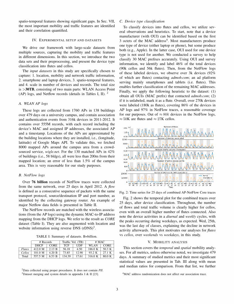
Fig. 2: Time series for 25 days of combined AP-NetFlow Core traces

Fig. 2 shows the temporal plot for the combined traces over25 days, after device classification. Throughout, the numberof flows and total traffic volume is clearly higher for cellos,even with an overall higher number of flutes connected. Alsonote the device activities in a diurnal and weekly cycles, withthe peaks occurring during weekdays, as expected. Wed, 25th,was the last day of classes, explaining the decline in networkactivity afterwards. This plot motivates our analyses for flutesvs cellos, over weekends vs weekdays, in this study.

V. MOBILITY ANALYSIS

This section covers the temporal and spatial mobility analy-ses. For all metrics, unless otherwise noted, we investigate 479days. A summary of studied metrics and their most significantstatistical values are presented in Tab. III along with meanand median ratios for comparison. From that list, we further

4MAC address randomization does not affect our association trace.

3

TABLE II: NetFlow (top) and AP logs/DHCP (bottom) sample data

Start time Finish time Duration Source IP Destination IP Protocol Source port Destination port Packet count Flow size1334332274.912 1334332276.576 1.664 173.194.37.7 10.15.225.126 TCP 80 60482 157 217708

User IP User MAC AP name AP MAC Lease begin time Lease end time10.130.90.3 00:11:22:33:44:55 b422r143-win-1 00:1d:e5:8f:1b:30 1333238737 1333238741

TABLE III: General results for mobility. Upper values are for week-days and lower ones for weekends (in red color). LJM: maximumjump [m]; DIA: diameter [m]; TJM: total trajectory length [m];GYR: radius of gyration [m]; BLD: no. uniq. buildings; APC: accesspoint count; PDT: time spent at preferred building [minutes]; DLT:total session time at each building.

Flutes (F) Cellos (C) Ratio (C/F)µ mdn σ µ mdn σ µ mdn

LJM 435 296 813 178 1 624 0.409 0.003350 168 683 97 1 312 0.277 0.006

DIA 549 411 874 195 1 642 0.355 0.002425 179 739 107 1 338 0.252 0.006

TJM 1582 707 2336 378 1 1444 0.239 0.0011036 279 1793 252 1 1766 0.243 0.004

GYR 396 290 2725 321 191 3265 1.102 1.019330 248 1368 178 65.1 1800 1.247 1.4

BLD 5.4 3 5.6 1.8 1 2.1 0.811 0.6592.8 2 4.1 1.5 1 1.8 0.539 0.262

APC 11.8 6 13.3 3.7 2 4.8 0.333 0.3337.2 4 8.8 3 2 3.8 0.536 0.5

PDT 225 161 219 248 164 254 0.314 0.333223 135 272 278 189 292 0.417 0.5

DTL 316 235 302 316 217 305 1 0.92326 247 308 316 221 309 0.97 0.89

investigate in this section those metrics that show the mostinteresting or non-trivial differences between flutes and cellos.

0 6 12 18 24T (Time of day) [h]

0.0000

0.0005

0.0010

0.0015

0.0020

P(T)

Academic

0 6 12 18 24T (Time of day) [h]

0.0000

0.0005

0.0010

0.0015

0.0020

P(T)

Social

0 6 12 18 24T (Time of day) [h]

0.0000

0.0005

0.0010

0.0015

0.0020

P(T)

Administrativelaptopsmartphone

0 6 12 18 24T (Time of day) [h]

0.0000

0.0005

0.0010

0.0015

0.0020

P(T)

Library

Fig. 3: PDF Session start over time of the day.

A. Session start probability

A session is defined as the period between WLAN associ-ations. The distributions of session start times across the dayfor four building categories are depicted in Fig. 3. The starttimes of the Sessions match the periodic beginning of classes,but mainly in Academic buildings, where users move mostlyat the start and end of classes. In these places, activity dropssharply for cellos at 5pm, with considerable flutes activity until8pm. For Social and Library buildings, the probability of new

sessions remains higher for a few more hours into the evening,and the times users tend to leave are more spread out. Wedo not make similar observation during weekends, which isexpected when the day is, unlike weekdays, not governed by aclass schedule. For most visitors, the session start distributionsshow a smooth shape and no significant differences betweendevice types (omitted for brevity).

B. Radius of gyration

This metric, GY R, captures the size of the geospatial dis-persion of a device’s movements, denoted by rg and computedas rg = 1

N

∑Nk=1 ( ~rk − ~rs)2, where ~r1, ..., ~rN are positional

vectors of a device and ~rs is its center of gravity.Grouping devices by their rg after six months of obser-

vation, we look at its evolution since the first time they areobserved. Unsurprisingly (cf. [8]), after an initial transientperiod of about one week, this value stabilizes even acrossdifferent semesters (not shown).

We split the traces into weekdays and weekends, presentingthe distributions in Fig. 4a. For cellos, we notice a substantialreduction in their overall mobility whereas, for flutes, thisdifference is not so pronounced. This might be due to studentshaving fewer activities on weekends, a tendency to study at asingle building like a library, or just not carry their cellos; wewill revisit this aspect in Sec. VII. Flutes, being “always-on”devices, are able to capture movements at pass-by locations,dining areas, and bus stops and thus are better suited to capturethe fine-granular mobility of their users than cellos.

Despite the 8.1km2 area of the campus (approximate radiusof 1.42km), buildings with related fields of study (e.g. FineArts) are fairly clustered. Computing the distance between thek-nearest neighboring buildings, for k = 22 and k = 9 (averagenumber of visited buildings for flutes and cellos) the mediandistances are 295m and 172m, respectively. Due to their focuson classes, attending students have limited area of activity onweekdays, which explains the observed radius of gyration.

We also evaluated: (1) diameter DIA, the longest distancebetween any pair of ~rk points; (2) max jump LJM , the longestdistance between a pair of consecutive ~rk points; and (3) totaltrajectory length TJM , the sum of all trips made by a device.The distributions of these metrics are similar to Radius ofGyration and therefore not shown. Table III summarizes themost significant statistical values for these metrics.

C. Visitation preferences and interests

We count the number of unique buildings visited by a user,BLD, and define a preferred building as the location where adevice has spent most of its time in a given day, measured inminutes and referred to as PDT . We approximate the latter bythe formula tb =

∑Nbk=1 Sk, where tb is the time spent, Nb the

total number of sessions and S1...SN the time duration of each

4

0 300 600 900 1200rg [meters]

0.0

0.2

0.4

0.6

0.8

1.0CD

F

weekday laptopweekday smartphoneweekend laptopweekend smartphone

(a)

100 101 102 103 104

t [hour]100

101

102

S(t)

t0.20

t0.54t0.33

t0.59

laptopssmartphones

(b)Fig. 4: (a) Radius of gyration (rg for the device types). (b) Visitedlocations S (t). Vertical lines at 7, 120 and 240 days.

session at a building b, here referred as DLT . Interestingly,cellos have slightly longer stays but both have medians around2:40 hours. The similarity of the distributions, combined witha lower number of visited locations indicate that cellos areused mostly when users remain longer periods at places.

Fig. 4b highlights the differences between flutes and celloson the required time t to visit S(t) locations. After an initialexploration period of one week the rates of new visits changesimilarly for both device types, and new exploration rates showup at 120 and 240 days. These could be explained by theweekly schedules of the university as well as the usual lengthof a lecture term (≈ 4 months).

Fig. 5: Zipf’s plot on L visited access points.

We also consider the number of unique APs a deviceassociates with, APC, which provides a finer spatial resolutionthan the building level. Furthermore, the probability of findinga device at its L-th most visited access point is shown in Fig. 5.When taking buildings as aggregating points for location, thevalues become L−1.36 for cellos and L−1.16 for flutes. Theseapproximations validate previous work on human mobility [8],yet highlight differences between device types.

D. Sessions per building

To study AP utilization over time, we look at the sessionduration distribution, or session duration dispersal kernel P(t),depicted in Fig. 6. The smaller inner plots represent the samemetric, limited to four types of buildings.

We noted that the five-minute spikes correspond to defaultidle-timeout for the used WiFi routers. On the other hand,the knees at 1 and 2 hours could be explained by the typicalduration of classes. They are only noticeable at Academicbuildings (shown inside inner plots) and during weekdays (not

shown). This leads us to conclude that despite the differencesin distributions of device types, flutes and cellos presentcertain similarities in their usage, such as during classes. Todifferentiate pass-by access points, we examine all sequencesof three unique APs where all session durations are lowerthan 5 minutes (typical idle-timeout). We observed these APsclustered at buildings that also had major bus stops nearby.

1s 10s 5min 1h2h 24ht

10−8

10−7

10−6

10−5

10−4

10−3

10−2

10−1

P(t)

Laptop

1s 10s 5min 1h2h 24ht

10−8

10−7

10−6

10−5

10−4

10−3

10−2

10−1

P(t)

Smartphone

Administrative

Academic

Library

Social

Administrative

Academic

Library

Social

Fig. 6: Probability P (t) of session duration t.

VI. TRAFFIC ANALYSIS

In this section, we compare different traffic characteristics,across device types, time and space. For this purpose, we startwith statistical characterization of individual flute and celloflows. Next, we measure how these flows, put together, affectthe network patterns across APs and buildings. Finally, userbehavior is analyzed by monitoring weekly cycles, data rates,and active durations. By quantifying temporal and spatialvariations of traffic across device types, we make a case fornew models to capture such variations based on the mostrelevant attributes. Table IV summarizes the results.

0 2 4 6 8 100.00.10.20.30.40.50.60.70.80.91.0

CDF

weekday laptops phones 2.31 1.43 Med. 0.88 0.56 3.28 2.05

weekend laptops phones 1.16 0.54 Med. 0.12 0.01 2.16 1.48

weekday laptopweekday smartphoneweekend laptopweekend smartphone

(a) Packet processing rate of APs(millions per day)

10 4 10 3 10 2 10 1 100 101 102 1030.00.10.20.30.40.50.60.70.80.91.0

CDF

weekday laptops phones 1665.80 1035.96 Med. 581.89 365.60 2421.45 1555.62

weekend laptops phones 848.73 417.29 Med. 75.88 3.11 1663.00 1201.35

weekday laptopweekday smartphoneweekend laptopweekend smartphone

(b) Traffic load of APs(MB per day, log-scale)

10 4 10 3 10 2 10 1 100 101 1020.00.10.20.30.40.50.60.70.80.91.0

CDF

weekday laptops phones 204.92 53.23 Med. 80.00 5.52 301.85 109.05

weekend laptops phones 295.50 54.37 Med. 105.24 0.39 439.05 138.60

weekday laptopweekday smartphoneweekend laptopweekend smartphone

(c) User data consumption(MB per day, log-scale)

0 50 100 150 200 250 3000.00.10.20.30.40.50.60.70.80.91.0

CDF

weekday laptops phones 81.32 20.72 Med. 52.42 6.94 84.83 30.90

weekend laptops phones 97.30 17.27 Med. 68.18 1.83 97.39 32.37

weekday laptopweekday smartphoneweekend laptopweekend smartphone

(d) User active time(minutes per day)

Fig. 7: Distribution plots

5

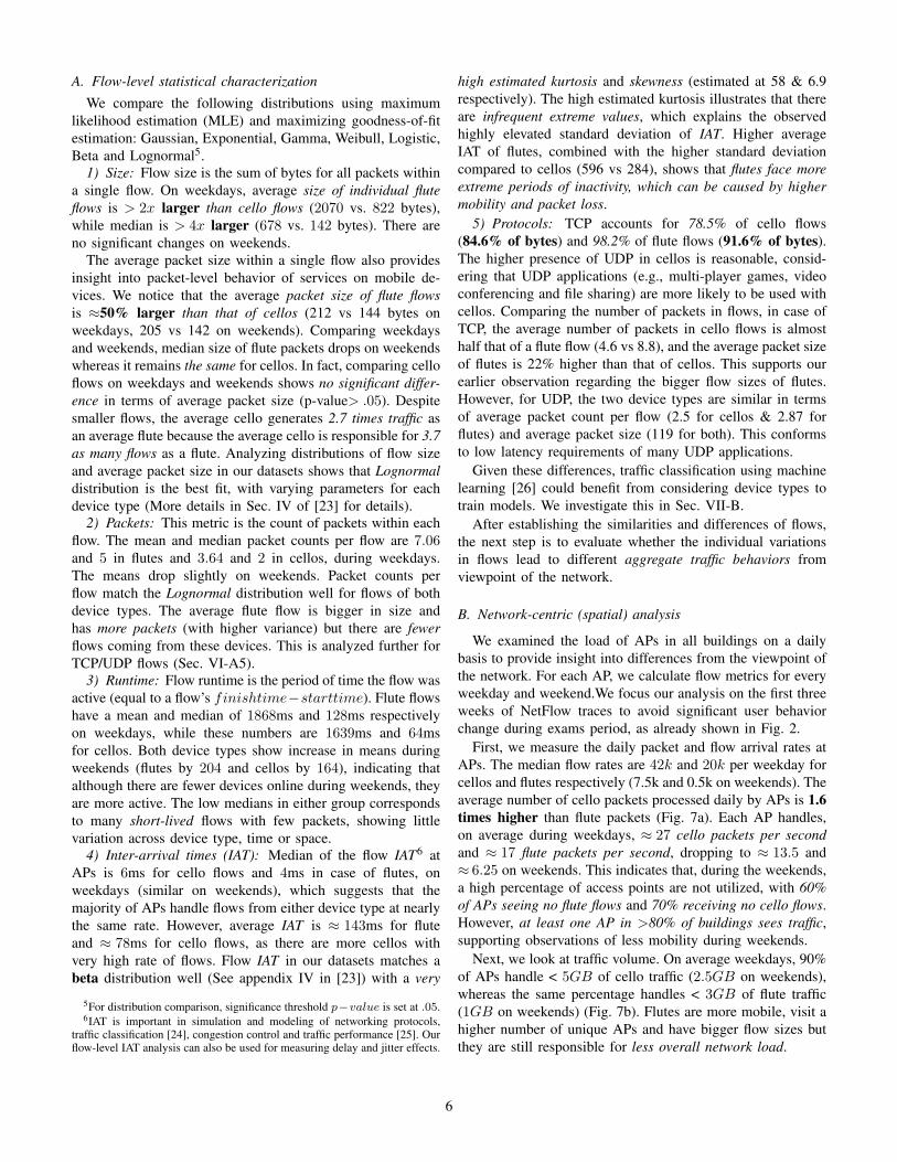
A. Flow-level statistical characterization

We compare the following distributions using maximumlikelihood estimation (MLE) and maximizing goodness-of-fitestimation: Gaussian, Exponential, Gamma, Weibull, Logistic,Beta and Lognormal5.

1) Size: Flow size is the sum of bytes for all packets withina single flow. On weekdays, average size of individual fluteflows is > 2x larger than cello flows (2070 vs. 822 bytes),while median is > 4x larger (678 vs. 142 bytes). There areno significant changes on weekends.

The average packet size within a single flow also providesinsight into packet-level behavior of services on mobile de-vices. We notice that the average packet size of flute flowsis ≈50% larger than that of cellos (212 vs 144 bytes onweekdays, 205 vs 142 on weekends). Comparing weekdaysand weekends, median size of flute packets drops on weekendswhereas it remains the same for cellos. In fact, comparing celloflows on weekdays and weekends shows no significant differ-ence in terms of average packet size (p-value> .05). Despitesmaller flows, the average cello generates 2.7 times traffic asan average flute because the average cello is responsible for 3.7as many flows as a flute. Analyzing distributions of flow sizeand average packet size in our datasets shows that Lognormaldistribution is the best fit, with varying parameters for eachdevice type (More details in Sec. IV of [23] for details).

2) Packets: This metric is the count of packets within eachflow. The mean and median packet counts per flow are 7.06and 5 in flutes and 3.64 and 2 in cellos, during weekdays.The means drop slightly on weekends. Packet counts perflow match the Lognormal distribution well for flows of bothdevice types. The average flute flow is bigger in size andhas more packets (with higher variance) but there are fewerflows coming from these devices. This is analyzed further forTCP/UDP flows (Sec. VI-A5).

3) Runtime: Flow runtime is the period of time the flow wasactive (equal to a flow’s finishtime−starttime). Flute flowshave a mean and median of 1868ms and 128ms respectivelyon weekdays, while these numbers are 1639ms and 64msfor cellos. Both device types show increase in means duringweekends (flutes by 204 and cellos by 164), indicating thatalthough there are fewer devices online during weekends, theyare more active. The low medians in either group correspondsto many short-lived flows with few packets, showing littlevariation across device type, time or space.

4) Inter-arrival times (IAT): Median of the flow IAT6 atAPs is 6ms for cello flows and 4ms in case of flutes, onweekdays (similar on weekends), which suggests that themajority of APs handle flows from either device type at nearlythe same rate. However, average IAT is ≈ 143ms for fluteand ≈ 78ms for cello flows, as there are more cellos withvery high rate of flows. Flow IAT in our datasets matches abeta distribution well (See appendix IV in [23]) with a very

5For distribution comparison, significance threshold p−value is set at .05.6IAT is important in simulation and modeling of networking protocols,

traffic classification [24], congestion control and traffic performance [25]. Ourflow-level IAT analysis can also be used for measuring delay and jitter effects.

high estimated kurtosis and skewness (estimated at 58 & 6.9respectively). The high estimated kurtosis illustrates that thereare infrequent extreme values, which explains the observedhighly elevated standard deviation of IAT. Higher averageIAT of flutes, combined with the higher standard deviationcompared to cellos (596 vs 284), shows that flutes face moreextreme periods of inactivity, which can be caused by highermobility and packet loss.

5) Protocols: TCP accounts for 78.5% of cello flows(84.6% of bytes) and 98.2% of flute flows (91.6% of bytes).The higher presence of UDP in cellos is reasonable, consid-ering that UDP applications (e.g., multi-player games, videoconferencing and file sharing) are more likely to be used withcellos. Comparing the number of packets in flows, in case ofTCP, the average number of packets in cello flows is almosthalf that of a flute flow (4.6 vs 8.8), and the average packet sizeof flutes is 22% higher than that of cellos. This supports ourearlier observation regarding the bigger flow sizes of flutes.However, for UDP, the two device types are similar in termsof average packet count per flow (2.5 for cellos & 2.87 forflutes) and average packet size (119 for both). This conformsto low latency requirements of many UDP applications.

Given these differences, traffic classification using machinelearning [26] could benefit from considering device types totrain models. We investigate this in Sec. VII-B.

After establishing the similarities and differences of flows,the next step is to evaluate whether the individual variationsin flows lead to different aggregate traffic behaviors fromviewpoint of the network.

B. Network-centric (spatial) analysis

We examined the load of APs in all buildings on a dailybasis to provide insight into differences from the viewpoint ofthe network. For each AP, we calculate flow metrics for everyweekday and weekend.We focus our analysis on the first threeweeks of NetFlow traces to avoid significant user behaviorchange during exams period, as already shown in Fig. 2.

First, we measure the daily packet and flow arrival rates atAPs. The median flow rates are 42k and 20k per weekday forcellos and flutes respectively (7.5k and 0.5k on weekends). Theaverage number of cello packets processed daily by APs is 1.6times higher than flute packets (Fig. 7a). Each AP handles,on average during weekdays, ≈ 27 cello packets per secondand ≈ 17 flute packets per second, dropping to ≈ 13.5 and≈ 6.25 on weekends. This indicates that, during the weekends,a high percentage of access points are not utilized, with 60%of APs seeing no flute flows and 70% receiving no cello flows.However, at least one AP in >80% of buildings sees traffic,supporting observations of less mobility during weekends.

Next, we look at traffic volume. On average weekdays, 90%of APs handle < 5GB of cello traffic (2.5GB on weekends),whereas the same percentage handles < 3GB of flute traffic(1GB on weekends) (Fig. 7b). Flutes are more mobile, visit ahigher number of unique APs and have bigger flow sizes butthey are still responsible for less overall network load.

6

Thus, the individual differences of flute and cello flowsresult in heterogeneous aggregate traffic patterns in time(different days) and space (APs at different buildings)7. Withthat established, in order to take steps towards modeling andsimulation, we also need to analyze the behavior of users.

C. User behavior (temporal) analysis

Here, we measure traffic patterns from a user-centric per-spective. We identified gaps in diurnal and weekly cycles (Fig.2) as well as traffic flow features of individual users includingdata consumption, packet rates, and network activity duration.

1) Data consumption: Fig. 7c shows daily data consump-tion, with 90% of cellos consuming < 700MB and 90% offlutes using < 200M on weekdays. Surprisingly, for cellos oncampus during weekends, average data consumption is evenhigher whereas data consumption of flutes drops sharply.

2) Packet rate: On weekdays, cellos on average generate≈318K packets, while flutes only average ≈84K packetsper day. On weekends, the few on-campus cellos see greatlyincreased number of packets, with an average daily packet rateof ≈ 495K. Weekend flutes also have a modestly increasedpacket count, with an average of ≈ 96K flows.

3) Active duration: Total active time of devices serves wellto demonstrate the differences between time spent online byusers of different device types. We rely on NetFlow to measure’active’ time instead of AP association time. This allows us todistinguish user’s idle presence in the network from its activityperiods. Cellos have 4x average active time compared to flutesin our traces (≈ 81 vs ≈ 21 min on weekdays, ≈ 97 vs ≈ 17min on weekends). Overall, 90% of cellos are active for <3.5hand 90% of flutes are active for <1h (Fig. 7d). As evident invarious metrics, the cellos appearing on weekends are moreactive than the average cello on weekdays.

Overall, the data consumption of flutes seems to be morebursty in nature, with bigger flows and lower active duration.This could be due to more intermittent usage of flutes andalso bundling of network requests to save battery on thesedevices. In addition, there are fewer devices on campus duringweekends, but those remaining devices are more active andconsume more data than average.

VII. INTEGRATED MOBILITY-TRAFFIC ANALYSIS

We study the relation between mobility and network trafficfeatures, examine whether their fusion provides a case for thenecessity of integrated mobility-traffic models, and introducesteps towards such models (Sec. VII-B).

A. Feature engineering

To simplify analysis and interpretation, and reduce di-mensionality, we identify the most important features. First,we study the relationships among variables from mobilityand traffic dimensions separately. Then, from this subset ofcombined features, we investigate whether clusters of userdevices appear in the dataset. For this, we use correlationfeature selection (CFS [27]), to obtain uncorrelated features,

7A more in-depth analysis is presented in appendix IV [23].

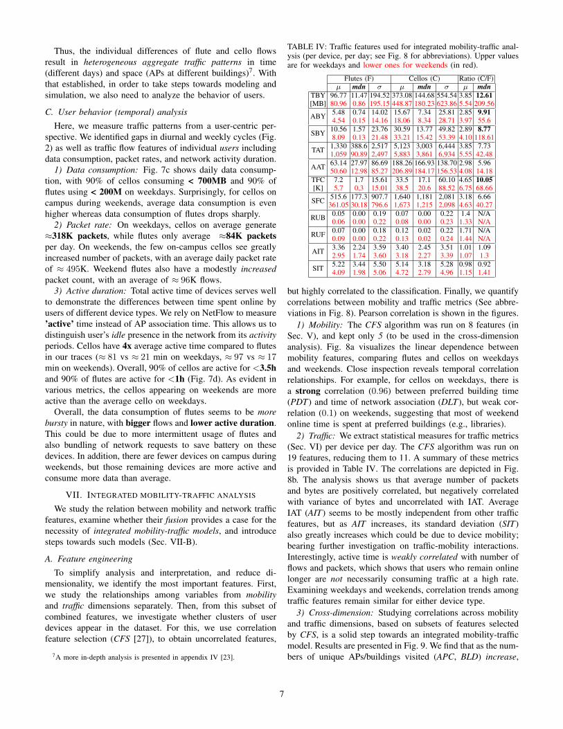
TABLE IV: Traffic features used for integrated mobility-traffic anal-ysis (per device, per day; see Fig. 8 for abbreviations). Upper valuesare for weekdays and lower ones for weekends (in red).

Flutes (F) Cellos (C) Ratio (C/F)µ mdn σ µ mdn σ µ mdn

TBY[MB]

96.77 11.47 194.52 373.08 144.68 554.54 3.85 12.6180.96 0.86 195.15 448.87 180.23 623.86 5.54 209.56

ABY 5.48 0.74 14.02 15.67 7.34 25.81 2.85 9.914.54 0.15 14.16 18.06 8.34 28.71 3.97 55.6

SBY 10.56 1.57 23.76 30.59 13.77 49.82 2.89 8.778.09 0.13 21.48 33.21 15.42 53.39 4.10 118.61

TAT 1,330 388.6 2,517 5,123 3,003 6,444 3.85 7.731,059 90.89 2,497 5,883 3,861 6,934 5.55 42.48

AAT 63.14 27.97 86.69 188.26 166.93 138.70 2.98 5.9650.60 12.98 85.27 206.89 184.17 156.53 4.08 14.18

TFC[K]

7.2 1.7 15.61 33.5 17.1 60.10 4.65 10.055.7 0.3 15.01 38.5 20.6 88.52 6.75 68.66

SFC 515.6 177.3 907.7 1,640 1,181 2,081 3.18 6.66361.05 30.18 796.6 1,673 1,215 2,098 4.63 40.27

RUB 0.05 0.00 0.19 0.07 0.00 0.22 1.4 N/A0.06 0.00 0.22 0.08 0.00 0.23 1.33 N/A

RUF 0.07 0.00 0.18 0.12 0.02 0.22 1.71 N/A0.09 0.00 0.22 0.13 0.02 0.24 1.44 N/A

AIT 3.36 2.24 3.59 3.40 2.45 3.51 1.01 1.092.95 1.74 3.60 3.18 2.27 3.39 1.07 1.3

SIT 5.22 3.44 5.50 5.14 3.18 5.28 0.98 0.924.09 1.98 5.06 4.72 2.79 4.96 1.15 1.41

but highly correlated to the classification. Finally, we quantifycorrelations between mobility and traffic metrics (See abbre-viations in Fig. 8). Pearson correlation is shown in the figures.

1) Mobility: The CFS algorithm was run on 8 features (inSec. V), and kept only 5 (to be used in the cross-dimensionanalysis). Fig. 8a visualizes the linear dependence betweenmobility features, comparing flutes and cellos on weekdaysand weekends. Close inspection reveals temporal correlationrelationships. For example, for cellos on weekdays, there isa strong correlation (0.96) between preferred building time(PDT) and time of network association (DLT), but weak cor-relation (0.1) on weekends, suggesting that most of weekendonline time is spent at preferred buildings (e.g., libraries).

2) Traffic: We extract statistical measures for traffic metrics(Sec. VI) per device per day. The CFS algorithm was run on19 features, reducing them to 11. A summary of these metricsis provided in Table IV. The correlations are depicted in Fig.8b. The analysis shows us that average number of packetsand bytes are positively correlated, but negatively correlatedwith variance of bytes and uncorrelated with IAT. AverageIAT (AIT) seems to be mostly independent from other trafficfeatures, but as AIT increases, its standard deviation (SIT)also greatly increases which could be due to device mobility;bearing further investigation on traffic-mobility interactions.Interestingly, active time is weakly correlated with number offlows and packets, which shows that users who remain onlinelonger are not necessarily consuming traffic at a high rate.Examining weekdays and weekends, correlation trends amongtraffic features remain similar for either device type.

3) Cross-dimension: Studying correlations across mobilityand traffic dimensions, based on subsets of features selectedby CFS, is a solid step towards an integrated mobility-trafficmodel. Results are presented in Fig. 9. We find that as the num-bers of unique APs/buildings visited (APC, BLD) increase,

7

weekend  

weekday  flutes   cellos   Abbr. Description

TBY Total flow bytesABY Avg. flow bytesSBY Std. flow bytesTAT Total active timeAAT Avg. active timeTFC Total flow countSFC Std. flow countsRUB UDP bytes / total

bytesRUF UDP flows / total

flowsAIT Avg. IATSIT Std. IAT

Abbr. DescriptionAPC AP Count (unique)PDT Preferred building

∆tTJM Total (sum) jumpsDIA Diameter of mobilityDLT Delta time (time of

network association)(a) Mobility (b) Traffic

Fig. 8: Correlation plots for (a) mobility and (b) traffic features. Each cell’s left half is for flutes and right half is for cellos, the upper righttriangle is for weekdays and the lower left for weekends.

Fig. 9: Correlation plots of mobility vs. traffic on weekdays (top) vs.weekends (bottom) for flutes (left) and cellos (right).

the average active time (AAT), and total and std. of flowcounts (TFC and SFC) decrease markedly (significant negativecorrelation). Surprisingly, there is no noticeable change in totaltraffic consumed with change in APC, suggesting bundlingof more packets in flute flows. (Similar correlation betweenmobility diameter and the above traffic features) Average IAT(AIT) of flutes also rises slightly as mobility metrics decrease;for cellos this correlation is almost nonexistent. This reinforcesour “stop-to-use” categorization; cellos are movable but arenot active in transit. To sum, flutes score high on mobilitymetrics, have an overall lower flow count and network trafficbut produce bigger flows on average. For cellos, on weekendsthe more time spent at preferred buildings the higher the totalactive time (TAT) and flow counts; this effect exists to a lesserdegree for flutes. On weekdays, such correlation does not exist.

B. Steps towards modeling

Here we present our steps towards an integrated mobility-traffic model, with various applications in simulation and pro-tocol design. We utilize daily mobility and traffic features ofusers during a week. First, we examine how different mobilityand traffic features are for flutes and cellos using machinelearning. Second, we investigate whether natural convex clus-ters of users appear in the dataset. These steps verify that the

differences of mobility and traffic characteristics across devicetypes are significant. We also find that combining mobilityand traffic makes this distinction even more clear. Finally,mixture models are used to model and synthesize simulateddata points of each device type, finding that the accuracy themixture model increases when trained on combined features.

1) Supervised classification: Having shown significant dif-ferences throughout this study, we used support vector ma-chines (SVM) on different subsets of features to examine thefeasibility of device type inference as well as the relationshipbetween mobility and traffic characteristics. These sets includemobility and traffic features separately, then combined, andthen combined with weekend/weekday labels. Using solely mo-bility features achieves ≈65% accuracy, while traffic featuresalone, obtains ≈79% accuracy. Using all mobility and trafficvariables combined, the trained model achieves ≈81% accu-racy. Then, as the combined feature set is extended to includeweekdays and weekends independently, accuracy increases to≈86%. This suggests that users’ behavior (both flutes andcellos) is more distinguishable when looking at combinedmobility and traffic features; especially when temporal featuressuch as weekdays are considered separately from weekends.We note that such behavior gaps are not the same for bothdevice types and a model should to take that into account.

2) Unsupervised clustering: To investigate natural convexclusters, we used K-means algorithm. Using mobility featuresonly, the best mean silhouette coefficient is achieved on k=2and 4. However, cluster sizes are highly skewed and at k=2, ≈60% of devices are correctly clustered. Traffic features alone,at k=2, results in ≈ 81.2% accuracy. Combining mobility andtraffic, increases the accuracy to ≈ 81.5%. While some flutesand cellos are similar in terms of mobility and traffic, theclusters of the combined features clearly illustrate two distinctmodes (especially in traffic) and the high homogeneity of theclusters hints at disjoint sets of behaviors in mobility andtraffic dimensions, governed by the device type.

8

3) Mixture model: To take a step towards synthesis of tracesbased on our datasets, we trained Gaussian mixture models(GMM) on combined mobility and traffic features. Fromthe combined model (CM ), we acquired simulated samples.We used Kolmogorov-Smirnov (KS) statistic to compare thesimulated samples with the real data and found that CM isable to capture the behaviors of each device type. (AverageKS statistic of features is ≈ 0.15 for flutes and ≈ 0.14for cellos. More details in appendix V [23].) Importantly,the combined model produces samples whose traffic featuresmatch the original data better, compared with training a GMMon traffic features alone (based on KS statistic), hinting ata key relationship between mobility and traffic. However,comparing mobility features of CM with a GMM trained onmobility features alone shows no improvement.

Overall, this suggests that there is significant potential for anintegrated mobility-traffic model that captures the differencesand relationships of features, across device types, time andspace. We leave detailed comparison of combined modelingwith separate modeling of mobility and traffic for future work.

VIII. CONCLUSION

In this study, we mine large-scale WLAN and NetFlow logsfrom a campus to answer: (I) How different are mobility andtraffic characteristics across device types, time and space? (II)What are the relationships between these characteristics? (III)Should new models be devised to capture these differences?And, if so, how? We build FLAMeS, a framework for sys-tematic processing and analysis of the datasets. Using MACaddress survey, OUI matching and web domain analysis, wecategorized devices: flutes (“on-the-go”) and cellos (“stop-to-use”). We then study a multitude of mobility and trafficmetrics, comparing flutes and cellos across time and space.On average, flutes visit twice as many APs as cellos, whilecellos generate ≈2x more flows. However, flute flows are2.5x larger in size, with ≈2x the number of packets. Thebest fit distribution for location preference is Zipfian, forflow/packet sizes is Lognormal, and for flow IAT at APsis beta. Furthermore, flute traffic drops sharply on weekendswhereas many cellos remain active. Across mobility and trafficdimensions, we spot a negative correlation for flutes betweenmobility and flow duration but negligible correlation withtraffic size; for cellos, this effect is less pronounced. Wefind a negative correlation with APs visited and active time,particularly for flutes. However, no correlation exists betweenAPs visited and traffic for cellos. We quantified correlationsacross both mobility and traffic. Finally, we applied machinelearning and trained a mixture model to synthesize data pointsand verified that the combined mobility-traffic features capturethe differences in metrics better than either mobility or trafficseparately. Many of our findings are not captured by today’smodels, and they provide insightful guidelines for the designof evaluation frameworks and simulations models. Hence, thisstudy answered the questions posed, introduced a strong casefor newer models, and provided our first step towards a futureintegrated mobility-traffic model.

Acknowledgments: We thank Alin Dobra for help in the com-puting cluster, and the anonymous reviewers for useful feedback.Mostafa Ammar suggested the term ’cello mobility’. Partial fundingwas provided by NSF 1320694 at Univ. of Florida, August-WilhelmSheer fellowship at Technical University-Munich, and Aalto Univ.

REFERENCES

[1] J. Treurniet, “A Taxonomy and Survey of Microscopic Mobility Modelsfrom the Mobile Networking Domain,” ACM CSUR, 2014.

[2] A. Hess, K. A. Hummel, W. N. Gansterer, and G. Haring, “Data-drivenHuman Mobility Modeling: A Survey and Engineering Guidance forMobile Networking,” ACM CSUR, 2016.

[3] D. Kotz and K. Essien, “Analysis of a Campus-Wide Wireless Network,”Springer Wireless Networks, vol. 11, no. 2, January 2005.

[4] T. Henderson, D. Kotz, and I. Abyzov, “The changing usage of a maturecampus-wide wireless network,” Elsevier Computer Networks, 2008.

[5] G. Maier, F. Schneider, and A. Feldmann, “A First Look at MobileHand-held Device Traffic,” in Proc. of IEEE PAM, 2010.

[6] Y. Zhand and A. Arvidsson, “Understanding the Characteristics ofCellular Data Traffic,” in ACM SIGCOMM CellNet workshop, 2012.

[7] S. Moghaddam and A. Helmy, “SPIRIT: A simulation paradigm forrealistic design of mature mobile societies,” in IWCMC ’11, 2011.

[8] M. C. Gonzalez, C. A. Hidalgo, and A.-L. Barabasi, “Understandingindividual human mobility patterns,” Nature, vol. 453, no. 7196, 2008.

[9] C. Song, T. Koren, P. Wang, and A.-L. Barabási, “Modelling the scalingproperties of human mobility,” Nature Physics, vol. 6, no. 10, 2010.

[10] D. Zhang, J. Huang, Y. Li, F. Zhang, C. Xu, and T. He, “Exploringhuman mobility with multi-source data at extremely large metropolitanscales,” MobiCom ’14.

[11] G. Maier, F. Schneider, and A. Feldmann, “A first look at mobile hand-held device traffic,” in PAM ’10. Springer, 2010.

[12] U. Kumar, J. Kim, and A. Helmy, “Changing patterns of mobile network(WLAN) usage: Smart-phones vs. laptops,” IWCMC ’13, 2013.

[13] X. Chen, R. Jin, K. Suh, B. Wang, and W. Wei, “Network performance ofsmart mobile handhelds in a university campus wifi network.” IMC’12.

[14] A. Gember, A. Anand, and A. Akella, “A comparative study of handheldand non-handheld traffic in campus wi-fi networks,” in PAM ’11.

[15] M. Afanasyev, T. Chen, G. M. Voelker, and A. C. Snoeren, “Analysis of amixed-use urban wifi network: when metropolitan becomes neapolitan,”in ACM SIGCOMM ’08.

[16] I. Papapanagiotou, E. M. Nahum, and V. Pappas, “Smartphones vs.laptops: comparing web browsing behavior and the implications forcaching,” SIGMETRICS’12.

[17] H. Falaki, D. Lymberopoulos, R. Mahajan, S. Kandula, and D. Estrin,“A first look at traffic on smartphones,” IMC ’10, 2010.

[18] A. K. Das, P. H. Pathak, C.-N. Chuah, and P. Mohapatra, “Characteri-zation of wireless multidevice users,” ACM TOIT, 2016.

[19] P. Cao, G. Li, A. Champion, D. Xuan, S. Romig, and W. Zhao, “Onhuman mobility predictability via wlan logs,” in INFOCOM ’17.

[20] A. Nikravesh, Y. Guo, F. Qian, Z. M. Mao, and S. Sen, “An in-depthunderstanding of multipath TCP on mobile devices,” in MobiCom ’16.

[21] X. G. Meng, S. H. Y. Wong, Y. Yuan, and S. Lu, “Characterizing flowsin large wireless data networks,” MobiCom ’04, 2004.

[22] F. Xu, Y. Li, H. Wang, P. Zhang, and D. Jin, “Understanding mobiletraffic patterns of large scale cellular towers in urban environment,”IEEE/ACM Transactions on Networking, April 2017.

[23] “Analyzing Mobility-Traffic Correlations in Large WLAN Traces:Flutes vs. Cellos.” [Online]. Available: https://arxiv.org/abs/1801.02705

[24] A. W. Moore and D. Zuev, “Internet traffic classification using bayesiananalysis techniques,” SIGMETRICS ’05, vol. 33, no. 1, 2005.

[25] V. Paxson and S. Floyd, “Wide area traffic: the failure of Poissonmodeling,” IEEE/ACM ToN, vol. 3, no. 3, jun 1995.

[26] T. Nguyen and G. Armitage, “A survey of techniques for internet trafficclassification using machine learning,” IEEE CST’08.

[27] M. A. Hall, “Correlation-based feature selection for machine learning,”Ph.D. dissertation, The University of Waikato, 1999.

[28] W.-J. Hsu, T. Spyropoulos, K. Psounis, and A. Helmy, “Modeling time-variant user mobility in wireless mobile networks.”

[29] P. Widhalm, Y. Yang, M. Ulm, S. Athavale, and M. C. González, “Dis-covering urban activity patterns in cell phone data,” Transportation’15.

[30] C. Boldrini and A. Passarella, “Hcmm: Modelling spatial and temporalproperties of human mobility driven by users’ social relationships,”Computer Communications, vol. 33, no. 9, 2010.

9