Health and Safety Executive

Fluid structure interaction effects on and dynamic response of pressure vessels and tanks subjected to dynamic loading

Prepared by The Steel Construction Institute for the Health and Safety Executive 2007

RR527 Research Report

Health and Safety Executive

Fluid structure interaction effects on and dynamic response of pressure vessels and tanks subjected to dynamic loading Part 1: State-of-the-art review

The Steel Construction Institute Silwood Park Ascot Berks SL5 7QN

As part of a suite of work looking at fluid interaction effects on (and the dynamic response of ) pressure vessels and tanks subjected to dynamic loading, this report details the findings of a state-of-the-art review of the available literature, to consider analysis methodologies, dynamic loads and simplified procedures for the determination of the response of tanks and pressure vessels subjected to strong vibration. Strong vibration is defined as the shaking of a structure resulting from earthquake, blast or ship impact. The response of a tank/vessel under strong vibration can be split into three hydrodynamic components and simplified procedures exist for determining the response of fixed-base, vertical, cylindrical tanks/vessels. For other tank/vessel types, linear/non-linear finite element dynamic analyses need to be used, as no simple solution for the various hydrodynamic components are available.

This report and the work it describes were funded by the Health and Safety Executive (HSE). Its contents, including any opinions and/or conclusions expressed, are those of the authors alone and do not necessarily reflect HSE policy.

HSE Books

© Crown copyright 2007

First published 2007

All rights reserved. No part of this publication may bereproduced, stored in a retrieval system, or transmitted inany form or by any means (electronic, mechanical,photocopying, recording or otherwise) without the priorwritten permission of the copyright owner.

Applications for reproduction should be made in writing to:Licensing Division, Her Majesty’s Stationery Office,St Clements House, 2-16 Colegate, Norwich NR3 1BQor by e-mail to hmsolicensing@cabinet-office.x.gsi.gov.uk

ii

CONTENTS

EXECUTIVE SUMMARY VI

1 INTRODUCTION 11.1 BACKGROUND 11.2 OBJECTIVES OF STUDY 11.3 SCOPE OF STUDY 2

2 STATE-OF-THE-ART REVIEW OF ANALYSIS METHODOLOGIES FORPRESSURE VESSELS AND TANKS ON TOPSIDES 32.1 INTRODUCTION 32.2 METHODOLOGIES FOR ANALYSIS OF PRESSURE VESSELS AND TANKS

ON TOPSIDES 42.3 SIMPLIFIED UNCOUPLED ANALYSIS 62.4 COUPLED ANALYSIS AND UNCOUPLED ANALYSIS USING DECK

RESPONSE SPECTRA 6

2.4.1 UNCOUPLED ANALYSIS USING DECK RESPONSE SPECTRA 9

2.4.2 COUPLED ANALYSIS 112.5 SUMMARY OF FINDINGS ON ANALYSIS METHODOLOGIES 11

3 REVIEW OF LOADING ON PRESSURE VESSELS AND TANKS ON TOPSIDESFROM LATERAL EXCITATION 123.1 INTRODUCTION 123.2 EARTHQUAKE LOADING 12

3.2.1 DESCRIPTION OF EARTHQUAKE LOADING 12

3.2.2 EARTHQUAKE RESPONSE SPECTRA FOR ANALYSIS OF OFFSHORE

PLATFORMS 13

3.2.3 SECONDARY EARTHQUAKE RESPONSE SPECTRA FOR ANALYSIS OFEQUIPMENT ON TOPSIDES 13

3.3 BLAST LOADING 14

3.3.1 DESCRIPTION OF BLAST LOADING 14

3.3.2 DECK RESPONSE SPECTRA FOR BLAST LOADING 143.4 LOADING ON PRESSURE VESSELS/TANKS FROM SHIP IMPACT 15

3.4.1 DESCRIPTION OF SHIP IMPACT LOADING 16

3.4.2 DECK RESPONSE SPECTRA FOR SHIP IMPACT LOADING 173.5 COMPARISON OF EARTHQUAKE, BLAST AND SHIP IMPACT

SECONDARY RESPONSE SPECTRA 183.6 SUMMARY OF FINDINGS ON LOADING ON TOPSIDES FROM

EARTHQUAKE, BLAST AND SHIP IMPACT 19

4 FLUID-STRUCTURE INTERACTION AND DYNAMIC RESPONSE OF PRESSUREVESSELS/TANKS UNDER LATERAL EXCITATION 204.1 INTRODUCTION 20

iii

4.2 DESCRIPTION OF RESPONSE OF PRESSURE VESSELS AND TANKS 204.3 VERTICAL CYLINDRICAL FIXED BASE TANKS/VESSELS 22

4.3.1 CONVECTIVE COMPONENT 22

4.3.2 RIGID IMPULSIVE COMPONENT 24

4.3.3 FLEXIBLE IMPULSIVE COMPONENT 264.4 RECTANGULAR FIXED BASE TANKS 29

4.4.1 CONVECTIVE COMPONENT 29

4.4.2 RIGID IMPULSIVE COMPONENT 31

4.4.3 FLEXIBLE IMPULSIVE COMPONENT 324.5 FIXED BASE HORIZONTAL CIRCULAR CYLINDRICAL TANKS/VESSELS 324.6 TANKS WITH INTERNAL BAFFLES 344.7 ROCKING RESPONSE OF VESSELS/TANKS 354.8 COMBINATION OF PRESSURES AND RESULTANT STRESSES 364.9 SUMMARY OF DYNAMIC RESPONSE OF VESSELS/TANKS UNDER

LATERAL EXCITATION 37

5 CONCLUSIONS 39

6 REFERENCES 40

iv

EXECUTIVE SUMMARY

A state-of-the-art review was carried out on the analysis methodologies, dynamic loads and simplified procedures for the determination of the response of tanks and pressure vessels under strong vibration.

Strong vibration is defined as the strong shaking of a structure as may occur under dynamic loadings such as earthquake, blast and ship impact. This review covered the relevant offshore and nuclear codes of practice in addition to recent technical papers.

The strong vibration phenomenon is explicitly addressed in ISO/CD 19901-3 [4] where it is recommended that depending on the exposure level of the platform, all new installations or reassessment of existing installations be designed for the effects of strong vibration. The recommended approach for determining the response of deck appurtenances and equipment to strong vibration is based on whether the component can be classified as rigid or flexible. For rigid equipment, simplified uncoupled procedures can be used. Flexible or compliant equipment require the use of coupled analyses or uncoupled analyses using deck (or secondary) response spectra.

The dynamic loading from strong vibration can result from earthquake, blast and ship impact. The frequency content of the loading from these excitations is different and it was found that the peak values from blast and ship impact loading generally occur at higher frequencies than that from earthquake loading. In addition, it was noted that compared to onshore spectra, sea-floor spectra exhibit lower peak vertical and comparable peak horizontal accelerations although at different frequencies.

The response of a tank/vessel under strong vibration can be split into 3 hydrodynamic components termed convective or sloshing component, rigid-impulsive component and flexible-impulsive component. The frequencies associated with sloshing are usually quite low and generally only the first sloshing frequency is considered for design purposes. The rigid-impulsive component is due to rigid body motion of the fluid and is subjected to the maximum ground acceleration. The flexible-impulsive component accounts for the flexibility of the tank/vessel and is subjected to the acceleration pertaining to the relevant modes of vibration of the tank/fluid system.

It was found that simplified procedures exist for determining the response of fixed base vertical cylindrical tanks/vessels. For other tank types (rectangular, horizontal cylindrical), resort must be mode to linear/non-linear finite element dynamic analyses as no simple solution for all the hydrodynamic components are available.

Part 2 of the report will describe the numerical studies and results for the dynamic response of a typical pressure vessel on topsides under earthquake, ship impact and blast loading.

v

vi

1 INTRODUCTION

1.1 BACKGROUND

The Piper Alpha disaster in 1988, which resulted in fatalities, led to a complete re-assessment of safety on offshore platform structures. Lord Cullen in his subsequent report [1] on the disaster identified ‘strong vibration’ as a major issue, which may have led to the failure of emergency systems. Strong vibration is defined as the strong shaking of the structure which can occur following blast loading, earthquakes, ship impacts or dropped objects that may result in breakdown or failure of appurtenances and equipment such as emergency shutdown systems, fire protection systems, pressure vessels and tanks. Such failures can lead to escalation effects and delay mitigation measures resulting in partial or total collapse of the structure.

The phenomenon of strong vibration has been the subject of several studies since the issue was raised in Lord Cullen’s report and has led to the extension of the Health and Safety at Work Act 1974 to include strong vibration hazards offshore. The Safety Case Regulations (SCR) 1992 [2] requires that all potential hazards that may lead to a major accident are identified and defines a major accident as ‘any event involving major damage to the structure of the installation or plant affixed thereto’. The risks associated with such major accidents must be reduced to as low as reasonably practicable (ALARP) through quantified risk assessment (QRA).

In the offshore industry, the main focus is usually directed at the design of the primary structure. A survey of suppliers of equipment to North Sea operators, carried out as part of an EATEC study [3], revealed that there were no specific vibration requirements set for the various equipments. However, the various items of equipment play a major role in ascertaining the overall safety of the structure and, as such, need to be designed for the loading scenarios expected during the lifetime of the structure.

The items of equipment considered in this study are pressure vessels and tanks on topsides. The various types of platform configurations that exist and the complexity of the fluid-structure interaction problem combined with the different fixity conditions of the equipments preclude the provision of standard simplified design guidelines. Instead, this study aims at providing an understanding of the loads that are associated with the strong vibration phenomenon and their subsequent treatment in the analysis of equipment on topsides. In addition, an assessment of the dynamic response of pressure vessels and tanks on topsides is carried out with particular regard to the quantification of the various hydrodynamic components governing the response under lateral excitation. Comparison against simplified codified procedures is also provided.

1.2 OBJECTIVES OF STUDY

This study is concerned with the loading and response of pressure vessels and storage tanks on topsides for both fixed jacket structures, jackups (mobile platforms) and floating platforms subjected to strong vibration. The main objectives of the study can be summarised as follows:

• Assess state-of-the-art practice with respect to design of pressure vessels and tanks on topsides against lateral excitation

• Provide guidance on modelling of tank-liquid and vessel-liquid systems

• Quantify the relative importance of the hydrodynamic components on the dynamic behaviour of pressure vessels and tanks

1

• Assess magnitude of linear sloshing response due to lateral excitation.

1.3 SCOPE OF STUDY

To achieve the above objectives, the study is split into several stages as follows:

(a) Conduct a review of current practice for design of pressure vessels and storage tanks on topsides. The review includes all relevant codes of practice and relevant technical papers from the offshore industry and also, where appropriate, reference is made to the nuclear codes of practice. The review will address both the loading (from earthquakes, blast and ship collisions) and the description and quantification of the dynamic response of pressure vessels and tanks.

(b) Carry out linear dynamic finite element analysis on typical pressure vessels and tanks on topsides to determine both structural and fluid response.

(c) Carry out linear dynamic finite element analyses to assess relative importance of various hydrodynamic components on response of pressure vessels and tanks. The contribution of the various components to the total response is expected to differ depending on the configuration and geometry of the vessel/tank, the frequency content of the loading and the fixity conditions.

Chapter 2 provides an overview of the state-of-the-art practices in the analysis methodologies for pressure vessels and tanks subject to lateral excitation. The various analysis methodologies for determining the response of the equipment are discussed in relation to their range of applicability. The loading on the equipment arising from earthquake, ship impact and blast is described in Chapter 3. The procedures for computing the response of various types of tanks and vessels are outlined in Chapter 4. Finally the findings from this study are described in Chapter 5.

2

2 STATE-OF-THE-ART REVIEW OF ANALYSISMETHODOLOGIES FOR PRESSURE VESSELS AND TANKS ON

TOPSIDES

2.1 INTRODUCTION

This chapter provides a review of the analysis methodologies for design of pressure vessels and storage tanks on topsides. Both relevant papers and codes are assessed and current design practice is reported. Due to the vast amount of work carried out in the nuclear industry regarding the design of equipment (alternatively referred to as secondary systems), reference is also made to relevant nuclear codes of practice. The design process encompasses the following:

• Modelling or analysis methodology for pressure vessels/tanks

• Loading definition and application on pressure vessels/tanks

• Dynamic response of the pressure vessels/tanks

The codes of practice reviewed as part of this study are as follows:

• ISO/CD 19901-3 – Petroleum and natural gas industries – Specific requirements for offshore structures – Part 3: Topsides structure [4]

• API RP 2A-WSD – Recommended Practice for Planning, Designing and Constructing Fixed Offshore Platforms – Working Stress Design [5]

• NORSOK Standard N-003 – Actions and Action Effects [6]

• NORSOK Standard N-004 – Design of Steel Structures [7]

• ISO/CD 19902 – Petroleum and Natural Gas Industries – Fixed Steel Offshore Structures [8]

• Guidelines for the Seismic Design of Oil and Gas Pipeline Systems – ASCE [9]

• Seismic Design of Storage Tanks, Recommendations of a New Zealand Study Group [10]

• Eurocode 8: Design Provisions for Earthquake Resistance of Structures – Silos, Tanks and Pipelines [11]

• Department of Energy (HMSO) – Offshore Installations: Guidance on design, construction and certification [12]

• ASCE 4-98 – Seismic Analysis of Safety-Related Nuclear Structures and Commentary [13]

• Committee on Nuclear Structures and Materials (ASCE) – Structural Analysis and Design of Nuclear Plant Facilities [14]

The subsequent sections in this chapter provide a review of the various procedures used in the analysis of pressure vessels and tanks subjected to lateral excitation. Description and quantification of the loading resulting from earthquake, blast and ship impacts are assessed in Chapter 3. Chapter 4 addresses the dynamic response of pressure vessels and tanks under lateral excitation and provides an overview of the various simplified procedures used to quantify the response for tanks/vessels of various configurations.

3

2.2 METHODOLOGIES FOR ANALYSIS OF PRESSURE VESSELS AND TANKS ON

TOPSIDES

The terminology used in this report follows that adopted in the offshore and nuclear industries. Primary and secondary structures (or systems) are used to designate the whole platform structure and the equipment (i.e. pressure vessels, storage tanks etc.) respectively. Deck response spectra (variation of acceleration with frequency at deck level of platform) are used interchangeably with secondary response spectra.

The strong vibration phenomenon is explicitly addressed in ISO/CD 19901-3 [4], which recommends that, depending on the exposure level of the platform, all new installations or reassessment of existing installations be designed for the effects of strong vibration. General guidelines are provided for the assessment of deck appurtenances and equipment and fall into two categories namely:

• Analytical methods – finite element analysis to determine magnitude and frequency of loading. The risk to the items of equipment is quantified by identifying their significant modes, amplitudes and frequencies of vibration and, if required, by detailed analysis. The code recognises the fact that the loading arising from strong vibration, particularly relating to ship impacts and blast loading, is difficult to estimate accurately. Only limited studies (EATEC study [3]) have been carried out to quantify the loading on topsides arising from strong vibration. This issue is addressed further in Chapter 3.

• Walkdown studies whereby safety-critical equipment are identified and a qualitative assessment of their adequacy to sustain strong vibration is carried out. The latter is not addressed in this report but details of walkdown assessments are provided in the Health and Safety Executive (HSE) report OTH 93 415 [15].

Although seismic events are part of the strong vibration phenomenon, recommendations relating to seismic resistance of deck equipment are dealt with separately in ISO/CD 19901-3 [4] and are similar to the guidelines provided in API RP 2A-WSD [5]. However, the analysis types defined for the seismic case can be equally applied to blast loading and ship impacts unless otherwise specified.

The approach to determining the response of deck appurtenances and equipment to seismic loads is based on whether the component can be classified as ‘rigid’ or ‘flexible’. Components are classified as rigid if they satisfy the following requirements

• Their horizontal natural frequencies of vibration fall in the high frequency tail region of the deck response spectra (earthquake loading only). For blast and ship impact, there is no clearly defined tail region as the spectral acceleration at high frequencies can be significantly higher than the maximum deck acceleration. In such cases, engineering judgement should be used to decide whether the equipment can be assumed to move in unison with deck motion.

• Their support is sufficiently stiff so as not to allow for any dynamic amplification

Such components can be treated through simplified uncoupled analysis i.e. with the equipment assumed to have negligible effect on the stiffness properties of the primary structure (mass usually accounted for by point mass representation). Components that do not meet the above requirements have to be designed either through coupled analyses or uncoupled (decoupled) analyses using secondary response spectra. Figure 1 provides a summary of the analysis methodologies, which are detailed in the following sub-sections.

4

Coupled Uncoupled

Uncoupled

Equipment

Classification of Equipment

Rigid Flexible

Analysis Analysis Using

Deck Response

Spectra or time

history Simplified

Analysis

Obtain

Forces/Moments

at Supports

Detailed FE

Model of

Primary

Structure and

Apply Loading Time

History or Response

Spectrum

Obtain

Forces/Moments,

Stresses at Nodal

Points in Equipment

and at Supports

Generate Deck

Response Spectra/time

history at Support Points

to Equipment

Apply loading to

Detailed FE Model

of Equipment

Obtain

Forces/Moments,

Stresses at Nodal

Points in Equipment

and at Supports

Figure 1 Analysis Methodologies For Equipment on Offshore Platforms

5

2.3 SIMPLIFIED UNCOUPLED ANALYSIS

For simplified uncoupled analysis, the equipment is generally modelled as a point mass at the appropriate centre of gravity. The supports are then designed for the resulting forces and moments from the dynamic loads. ISO/CD 19901-3 [4] recommends that the forces/moments be calculated from the following steps:

(d) Determine the significant modes of vibration of the primary structure and extract the acceleration at the equipment support for each mode

(e) Compute the equipment acceleration by multiplying the acceleration at the support from (a) by a dynamic magnification ratio and

(f) Multiply the equipment mass by equipment acceleration found in step (b) to obtain forces/moments

The code specifies that the above method cannot be applied to flexible equipment requiring multi-degree-of-freedom (MDOF) treatment. Usually, items of equipment with fundamental natural frequencies of vibrations exceeding 20 Hz (in the case of earthquake loads) can be designed using the simplified uncoupled approach. This is, however, not the case for pressure vessels and tanks where the fundamental frequencies of the hydrodynamic components generally lie in the lower frequency ranges.

2.4 COUPLED ANALYSIS AND UNCOUPLED ANALYSIS USING DECK RESPONSE

SPECTRA

Components that do not meet the above requirements have to be designed either through coupled or uncoupled analyses using deck response spectra. In a coupled analysis, the component is modelled together with the structure and the stresses in the item of equipment and forces at supports can be directly obtained. For an uncoupled analysis, deck response spectra have to be generated or time histories of displacements/accelerations obtained at the deck level. These are then applied as loads to a model of the component from which forces and stresses can be extracted.

The nuclear code ASCE 4-98 [13] provides clear guidelines as to the criteria for selection of coupled/uncoupled analyses for items of equipment. ASCE 4-98 [13] recommends that coupled analysis is not required if the equipment (or secondary system) satisfies the following requirements:

• Total mass of component is 1% or less of supporting primary structure. If components are identical and located together, their masses shall be lumped together.

• Stiffness of component supported at two or more points does not restrict movement of primary system and

• Static constraints do not cause significant redistribution of load in primary structure.

For tanks and vessels with single deck attachment (i.e. connected at one deck level only and with no significant separation between the support points so that the acceleration at the various points can be assumed to be the same), the selection of coupled analysis or uncoupled analysis is based on the frequency ratio and the modal mass ratio [13]. The frequency ratio is the ratio of the uncoupled modal frequency of the equipment to the uncoupled modal frequency of the primary structure. The modal mass ratio is defined numerically as [13]

6

M 2� � s , M pi = ( ) (1) 1 �cii M pi

where � ci is the mode vector value from the primary system’s modal displacement at the connection point to the equipment obtained from the ith mass (with respect to the primary structure mass matrix) normalised modal vector {� pi} and Ms is the total mass of the secondary system. From the numerical values of the frequency ratio and modal mass ratio, the selection of the type of analysis can be carried out based on Figure 2 [13].

Figure 2 Criteria for Selection of Analysis Type for Equipment Attached to Primary

System [13]

The definition of the models is as follows:

Model A: Uncoupled Analysis – In this model, the mass and stiffness of the equipment have negligible effect on the primary structure’s dynamic characteristics. The response (response spectrum or time history) of the primary structure at the attachment point to the equipment is obtained and subsequently applied to a model of the equipment to evaluate the forces/moments and stresses in the latter.

Model B: Uncoupled Analysis – This model is similar to Model A except for the fact that the inertial loads due to the equipment are significant enough to warrant inclusion in the modelling of the primary structure. This is generally achieved via representation as a point mass at the appropriate centre of gravity similar to the simplified uncoupled case. The response (response spectrum or time history) of the primary structure at the attachment point to the equipment is

7

obtained and subsequently applied to a model of the equipment to evaluate the forces/moments and stresses in the latter.

Model C: Coupled Analysis – In this model, both the mass and stiffness properties of the equipment have a significant influence on the dynamic characteristics of the primary structure. The equipment model is included in the analysis of the primary structure so that the forces/moments and stresses in the equipment can be obtained directly.

For frequency ratios close to 1.0 and modal mass ratios exceeding approximately 0.05, a coupled analysis is generally required. For frequency ratios greater than approximately 1.5 and higher modal mass ratios (usually exceeding 0.15), an uncoupled analysis (Model B) with the mass of the equipment accounted for is adequate. Model A usually applies for low frequency ratios (less than 0.5) and high modal mass ratios (exceeding approximately 0.15).

In the latter two cases, a coupled analysis is sometimes carried out particularly in cases where a more accurate and less conservative result is sought.

For tanks and vessels with multi-deck attachment (i.e. connected at two or more deck levels), the differential accelerations have to be accounted for in the analysis. ASCE 4-98 [13] provides guidelines for determining whether the interaction of the secondary system with the primary structure is significant enough to warrant a coupled analysis or whether a decoupled analysis is permissible.

The procedure requires the determination of the modal mass ratio (as for equipment with single attachment point), which provides a measure of the degree of interaction of the masses of the equipment and the supporting structure in various modes. Numerically, for a primary structure mode i and an equipment mode j, it is defined as

2 r ={� [ ]} (2) [ ]�ciij cj

where rij is the modal mass ratio, �ci is a subvector of the uncoupled primary structure’s ith

normalised modal vector comprising only of the connecting degrees of freedom (i.e. the degrees of freedom corresponding to the connection points between the equipment and the primary structure) and �cj is a matrix of secondary system participation factors consisting of one term for each of the connecting degree of freedom. The values of rij are computed for all combinations of the modes and Figure 2 can be used to determine the analysis type required based on the value of rij used for the x-axis. Models A and B in the figure pertain to uncoupled analyses and Model C requires coupled analysis as described for equipment with single point attachment.

In addition, multi-point attachments can result in static constraints resulting in redistribution of loads and causing an increase in the primary system’s modal frequencies. Generally, ASCE 4-98 recommends that if the ratio of the increased primary system’s natural frequency to the uncoupled frequency exceeds 1.1, a coupled analysis should be performed.

The procedure for carrying out uncoupled analysis for equipment with multi-point attachment differ from that for single point attachment as the effect of the differential accelerations mentioned earlier have to be accounted for. A method for the uncoupled analysis of equipment with multi-point attachments is described in reference [14]. The procedure requires the determination of secondary response spectra at the various support points between the primary structure and the equipment. The various spectra are subsequently enveloped to produce a set of upper-bound spectra that can be used in the analysis of the equipment. In addition, an analysis should be performed to determine the effect of differential boundary displacements on the

8

equipment. This can be achieved through a static analysis whereby the maximum relative support displacements are obtained from the prior response spectrum analysis and imposed on the supported equipment in the most unfavourable condition.

Alternatively, loading can obtained at the various support points and are subsequently applied to the equipment. The force/moments and stresses in the equipment can then be obtained directly from the analysis.

2.4.1 UNCOUPLED ANALYSIS USING DECK RESPONSE SPECTRA

Deck response spectra are required for uncoupled analyses in the frequency domain. The problems associated with the generation of deck response spectra on offshore structures have been summarised by Kost and Sharpe [16]:

• Uncertainties in the frequency content of the input loading

• Assumptions used in the modelling of the interaction between the component, structure, water and foundation stiffness

• Assumptions used in the modelling of the dynamic characteristics and energy absorption properties of the structure and

• Uncertainty in the representation of the non-linear stiffness and damping effects

Similar uncertainties and approximations exist in the analysis of equipment or secondary systems in nuclear structures. Detailed guidelines are provided for the generation of secondary response spectra (SRS) and time histories for uncoupled/decoupled analyses in ASCE 4-98 [13]. The secondary response spectra are generated from the linear time history accelerations at the deck or support equipment locations. The platform acts as a filter with peaks generally occuring at the frequencies corresponding to peaks on the ground motion and at the natural frequencies of the supporting structure as shown in Figure 3.

Figure 3 Structure Excitation and Response at Various Platform Levels

9

&& && x 2 and && In the figure, x g represents the ground acceleration and x1 , && x 3 are the resulting

accelerations at the first, second and upper levels respectively. The response spectra exhibit amplified response at a frequency corresponding to the natural frequency of the structure (period Ts). In general, other major peaks will be present and are associated with higher vibrational modes.

ASCE 4-98 [13] recommends that the secondary response spectra be broadened prior to use in the analysis of secondary systems. Broadening, i.e. widening of the peaks associated with structural frequencies is carried out to account for the effects of the various uncertainties as shown in Figure 4. Craig et. al. [17], in their discussion of the API RP 2A 20th Edition Update, discuss a similar approach with regard to the generation of deck response spectra for design of equipment on offshore structures. However, no guidance is provided as to the amount of peak broadening required. ASCE 4-98 [13] suggests that the peaks be broadened by ± 15% in the frequency domain. This concept is illustrated in Figure 4 [14] where fj is 15%.

In conjunction with the broadening, ASCE 4-98 [13] also allows for a 15% reduction in the peak amplitude provided that the secondary system damping does not exceed 10%. The reduction is associated with the probability of exceedance of the various uncertainties described above. Similar procedures, as adopted in the nuclear industry, can be used for generation of deck response spectra for equipment on offshore platforms. It is noted, however, that for offshore sites, the level of uncertainties, particularly in the spectra/time histories used for analysis of the structure, may be greater than for onshore sites.

Figure 4 Broadened Spectrum

A procedure for carrying out uncoupled analyses of equipment on offshore platforms has been proposed by Bea and Bowen [18] based on an approach developed by Biggs and Roesset [19]. The method uses a combination of empirical (based on analysis results of conventional platforms) and theoretical approaches to derive Acceleration Magnification Ratio (AMR) curves which provide the ratio of the maximum acceleration of the equipment mass to the acceleration

10

of the structure at the equipment support as a function of the equipment period to structure period. The AMR is dependent on the damping ratios of the equipment and the structure and is also based on the assumption that when the equipment period exceeds 1.25 the structure period, the acceleration experienced by the equipment is governed by the ground motion rather than the support acceleration. It is noted, however, that it does not account for any of the uncertainties mentioned previously with respect to peak broadening for secondary response spectra.

Generally, decoupled analysis using secondary response spectra usually results in higher forces/moments and stresses in the equipment and supports than an equivalent coupled analysis. This is because for a coupled case, exact resonance cannot occur as the resonant frequencies shift away from each other [14]. For the uncoupled case, it is possible for a natural frequency of vibration of the equipment to correspond exactly to a natural frequency of the structure thereby leading to a resonant behaviour.

2.4.2 COUPLED ANALYSIS

For coupled analysis, ASCE 4-98 [13] recommends that a refined model of the component and a simplified model (instead of a detailed model) of the supporting structure may be used. The simplified model of the structure should, however, capture the significant natural frequencies and modes of vibration at the equipment support locations. This is ascertained by comparing the secondary response spectra from the simplified model of the supporting structure to that of the detailed model of the supporting structure at the support locations.

2.5 SUMMARY OF FINDINGS ON ANALYSIS METHODOLOGIES

In summary, review of the relevant codes and papers related to design of equipment on topsides led to the following findings:

• Strong vibration is addressed in the ISO standard. Analytical methods and walkdown studies are described for the assessment of equipment on topsides.

• Offshore codes ISO 19901-3 [4] and API 2A WSD [5] provide guidelines for analysis of equipment under seismic loading. Similar procedures can, however, be used for blast loading and ship impacts.

• For rigid equipment, simplified uncoupled procedures can be used. Flexible or compliant equipment require the use of coupled analyses or uncoupled analyses using deck (or secondary) response spectra.

• In the nuclear industry, input and modelling uncertainties are accounted for by broadening the secondary response spectra at the peaks corresponding to the structural frequencies.

• For equipment with multi-point attachment, ASCE 4-98 [13] provides guidelines for the selection of the type of analysis. This requires the determination of the modal mass ratio and the frequency ratio.

11

3 REVIEW OF LOADING ON PRESSURE VESSELS AND TANKS ON TOPSIDES FROM LATERAL EXCITATION

3.1 INTRODUCTION

Strong vibration from earthquakes, blast and ship impact results in lateral excitation of the decks that support the pressure vessels and storage tanks. Dynamic amplification occurs as a result of the inherent flexibility of the platform structure and depends on the dynamic characteristics of the platform and on the frequency content of the applied loading. As a result, the equipment may be subjected to higher acceleration values than free-field accelerations depending on the ratio of the natural frequencies of the equipment to that of the supporting structure. This review will address the current practice for determining the loading on topsides due to earthquakes, blast and ship collision.

3.2 EARTHQUAKE LOADING

The loading on pressure vessels and tanks due to earthquake arises from the vibratory response of the supporting deck structure. It is not the aim of this review to investigate the derivation of earthquake spectra used in the analysis of offshore platforms but rather to assess their application in the loading of pressure vessels and tanks on topsides. However, owing to the obvious relationship between the base spectra and the loading at deck level, a brief description of earthquake spectra used in the offshore sector is provided.

3.2.1 DESCRIPTION OF EARTHQUAKE LOADING

The shape and intensity of the response spectrum or time history loading at a particular site are governed by several parameters as described in reference [20]. Guidelines for generation of earthquake spectra are provided in the following codes of practice:

• API RP 2A-WSD – Recommended Practice for Planning, Designing and Constructing Fixed Offshore Platforms – Working Stress Design [5]

• NORSOK Standard N-003 – Actions and Action Effects [6]

• ISO/CD 19902 – Petroleum and Natural Gas Industries – Fixed Steel Offshore Structures [8]

The codes recommend that the platform structure be assessed under two different level of earthquake intensity based on their probability of occurrence. ISO/CD 19902 [8] defines these two levels as the Strength Level Earthquake (SLE), associated with a ground motion which has a reasonable likelihood of not being exceeded at the site during the lifetime of the platform, under which the platform should sustain little or no damage and the Ductility Level Earthquake (DLE), associated with a rare intense earthquake – return period of usually 1 in 10000 years, where considerable damage is allowed without any loss of life and/or major environmental damage. Specific clauses are included regarding the effect of SLE and DLE on deck appurtenances and equipment. The code requires that all equipment shall be designed and supported such that SLE actions can be resisted and that under DLE, safety critical systems and equipment shall be designed to be functional during and after the DLE event.

12

3.2.2 EARTHQUAKE RESPONSE SPECTRA FOR ANALYSIS OF OFFSHORE

PLATFORMS

Typical spectra for use on offshore platforms are provided in the API [5] and NORSOK [6] codes. The API [5] code provides recommendations for the generation of offshore spectra, which involves seismotectonic and site characterisation, seismic exposure assessment, ground motion characterisation and design ground motion specification.

Generally offshore spectra are generated from earthquake forcing functions obtained or modified from onshore sites. However, Smith [21] reported that data gathered from the Seafloor Earthquake Measurement System (SEMS) Program showed that seafloor motions differed from ground motions from onshore sites. The study concluded that the peak vertical acceleration recorded on offshore sites was lower than that recorded from onshore sites but occur at equal frequencies while the horizontal accelerations exhibited comparable peaks with slight differences in frequencies. However, owing to the lack of sufficient data, a rigorous probabilistic analysis was not possible and the above conclusions can only be taken as indicative of a trend.

3.2.3 SECONDARY EARTHQUAKE RESPONSE SPECTRA FOR ANALYSIS OF

EQUIPMENT ON TOPSIDES

Deck response spectra can be generated from the acceleration response resulting from time-history analysis of the offshore platform structure. Only limited studies, e.g. EATEC [3], have been carried out to assess the acceleration response at deck levels of the structure. A typical deck response spectra, reproduced from the EATEC study, corresponding to a 1 in 10000 earthquake is shown in Figure 5.

The structure was representative of a fixed leg platform of the type commonly found in the North Sea and comprised of two deck levels in addition to a heliport. The acceleration spectrum exhibits amplification in regions where the structural frequencies are associated with high frequency content in the ground motion. Typically, for earthquake loading, this occurs in the lower frequency ranges (usually below 5 Hz).

13

Figure 5 Deck Response Spectra For a 1 in 10000 year Earthquake Loading [3]

3.3 BLAST LOADING

Blast loading on offshore structures results from the explosion of a mixture of hydrocarbon gas in air. The loading generated by the blast depends on several factors including the stochiometry of the hydrocarbon mixture, the ignition source location, the amount of congestion in the module and the amount of confinement. Blast generally results in two types of loading namely overpressure loading and drag loading. The latter is not addressed in this study as the focus is on lateral excitation of the platform, which is generally negligible in the case of drag loading.

3.3.1 DESCRIPTION OF BLAST LOADING

Explosion or blast loading as may arise from overpressure is caused by the increase in pressure that results from the expansion of combustion products. A typical idealised overpressure time history is shown in Figure 6 and is characterised by the rise time, peak overpressure and the area under the curve.

Figure 6 Idealised Overpressure Time History For Blast Loading [24]

Generation of the time history can be achieved through experimental modelling or from mathematical/numerical models. The complexity of the problem, however, implies that the loading generated can only be a best estimate of the actual loading. Renwick and Norman [22] reports on the differences found between experimental overpressure loading data from a full scale testing at the British Gas site at Spadeadam and theoretical overpressures derived by various explosion modelling agencies. They found that the theoretical models exhibited a wide scatter with significant underestimation of the peak overpressure (compared to the experimental data).

3.3.2 DECK RESPONSE SPECTRA FOR BLAST LOADING

Walker et. al. [23] studied blast-induced vibrations on topsides and suggested a response spectrum for the assessment of the ability of equipment to withstand severe vibration. The study considered the displacement and acceleration response at various locations on the deck structure from 3 overpressure time histories idealised to 1 bar with rise times of 0.1sec, 0.2sec and 0.3sec.

14

The results showed that the rise times did not have any significant impact on the peak response. In addition, the longer duration impulse resulted in maximum displacement at the remote locations whereas the shorter duration impulse led to larger maximum accelerations.

The authors noted that the acceleration response spectra generated at the remote locations could be used in the assessment of equipment to severe vibration. However, the above-mentioned authors did not address the issue of peak broadening and peak reduction as described in section 2.4.2. These issues still need to be addressed for offshore applications. A typical deck response spectrum from blast loading, reproduced from the EATEC study [3], is shown in Figure 7.

Figure 7 Deck Response Spectra For Blast Loading [3]

It is noted that the peak accelerations are higher and occur at higher frequencies than that corresponding to the earthquake secondary response spectrum. This implies that the various hydrodynamic components characterising the response of pressure vessels and tanks will have different relative contributions depending on the loading type.

3.4 LOADING ON PRESSURE VESSELS/TANKS FROM SHIP IMPACT

The problem of ship collisions with offshore platforms is generally addressed in terms of energy considerations. The dissipation of the impact energy in fixed platform structures may be achieved through the following processes [24]:

• Ship deformation and/or rotation

• Local deformation or denting of member

• Elastic/plastic bending of member

• Fendering device

• Local framing distortions of platforms

• Global sway of platform

The elastic vibrations of platforms arising from ship impacts are generally conservatively neglected in the energy dissipation formulation of a ship striking a platform structure. This

15

�

assumption leads to a conservative design for all the external platform members likely to be subjected to the impact forces. Petersen and Pedersen [25] argue that for the case of ships hitting small offshore structures, the elastic vibrations of the platform may be significant, particularly where the generalised masses of the ship and platform are of the same order of magnitude and the lowest period of vibration of the platform is comparable to the duration of the collision. In addition, offshore structures having small dynamic stiffness will also experience a significant level of platform vibrations.

3.4.1 DESCRIPTION OF SHIP IMPACT LOADING

The codes of practice generally adopt the energy approach for the determination of the impact forces acting on offshore structures. The relevant codes that address this particular issue are:

• API 2A WSD [5]

• ISO/CD 19902 [8]

• NORSOK N-003 [6]

The codes recommend that the kinetic energy of the vessel be calculated from

E = a 5 . 0 m v2 (3)

where m is the mass of the ship, v is the velocity of the ship at impact and a is the added mass coefficient which accounts for the hydrodynamic forces acting on the ship during the collision. A value of 1.1 is assumed for the added mass coefficient for bow/stern collision and 1.4 for broadside impacts. ISO/CD 19902 [5] specifies that the values pertain to large vessels (5000 tons displacement) and that for smaller vessels, the above values should be increased. Petersen and Pedersen [25] report that previous studies have shown that the value of the added mass coefficients also depends on the duration of the impact and the relation between the collision force and the deformation. The authors pointed out that for broadside collisions, the added mass of 40% of vessel mass is a reasonable approximation for very short duration impacts (approx. 0.5-1.0 sec). For longer durations, the value of the added mass coefficient for broadside collisions can approach 100% of the vessel mass.

NORSOK N-004 [7] specifies that equation (3) pertains to fixed offshore platforms and that for floating structures, the following equation should be taken as:

� vi � 21�

�-

v �2E = 0.5 (m + v ) a s s s

s (4) s m + a s1 + s

m + ai i

where ms and mi are the masses of the ship and installation respectively, as and ai are ship and installation added masses and vs and vi are the velocities of the ship and installation. The velocity of the installation is usually taken as zero. No values are, however, provided for the added masses to be used for the ship and the installation.

ISO/CD 19902 [8] also specifies that two energy levels should be used in the assessment of the platform structure namely a low energy level impact corresponding to a frequent occurrence and a high energy impact level corresponding to a rare event. Guidelines are provided for the selection of the vessel velocity at impact. For the low energy event, a value of 0.5m/s is

16

recommended while for the high energy impact level, a value of 2m/s is specified. However, no guidance is offered as to the amount of energy imparted to the offshore structure.

This issue is addressed in the Department of Energy document [12] where the total kinetic energy of the collision process is specified as 14MJ for broadside impacts and 11MJ for bow/stern impacts. The amount of energy imparted to the structure is taken to be equal to the total kinetic energy released or less depending on the relative stiffness of the vessel and structure. The guidance document recommends that for fixed steel structures, the amount of energy absorbed by the structure should not be less than 4MJ. No energy levels are specified for floating platform structures. In addition, no clear specifications are provided for determining the duration of the collision. Previous studies by EATEC [3] and Walker et. al. [24] have used values ranging from 0.097sec to 0.5sec. These values were based on the assumption of elastic displacement of the structure with a peak impact force of approximately of 30MN.

Detailed studies on the collision mechanics of vessels with offshore structures have been carried out by various researchers [25, 26, 27]. Collision models requiring numerical solutions have been proposed where the impacting ship is represented by non-linear springs and the variation of the added mass is accounted for. It is, however, beyond the scope of this study to assess the applicability of these models for loading on offshore platforms. Instead, the energy approach adopted by the codes of practice will be used in defining the loading time history from ship impacts. In this approach, the loading is specified in terms of a force time history based on the amount of energy imparted to the platform. The force time history is usually determined as a rectangular impulse with an assumed duration based on the magnitude of the energy.

3.4.2 DECK RESPONSE SPECTRA FOR SHIP IMPACT LOADING

Similar procedures to those described for the seismic and blast loading can be used for the case of vessel impact. Time histories of accelerations/displacements or secondary response spectra are generated at the supports to the equipment and depending on the magnitude and frequency content of the loading, the appropriate analysis type (i.e. quasi-static, coupled/decoupled) for design of the component and its supports can be selected.

A typical deck response spectrum from ship impact, reproduced from the EATEC study, is shown in Figure 8. Two impact scenarios were considered:

• SHIP 1 – Load applied steadily over 0.097sec then removed

• SHIP 2 – Load applied steadily over 0.4 sec then removed

The deck acceleration response spectra corresponding to these two impact scenarios exhibit comparable peak responses at nearly equal frequencies. The structural peaks occur at different frequencies and have different magnitudes compared to that from blast and earthquake loading. However, the displacement of the structure was higher for the second case owing to the longer duration of loading (more comparable to the bending frequency of vibration of the structure) which resulted in greater energy absorption in the structure. Due consideration should therefore be given to the relative displacement between the equipment and the primary structure as this may affect the required amount of clearance between the equipment and any adjacent part of the structure (similar effect may arise from blast and earthquake loading).

17

Figure 8 Deck Response Spectra For Ship Impact [3]

3.5 COMPARISON OF EARTHQUAKE, BLAST AND SHIP IMPACT SECONDARY RESPONSE SPECTRA

The secondary response spectra reproduced from the EATEC study were derived from a series of finite element analyses carried out on a typical fixed jacket structure. The structure comprised of two main decks and a helicopter deck supported on a fixed leg jacket. Earthquake, blast and ship impact time histories were applied at the appropriate levels and the acceleration response at various points on the platform was obtained.

A comparison of the secondary response spectra, as reproduced from the EATEC study [3], from the various loading types is shown in Figure 9. It is observed that:

• The secondary response spectra from blast loading and ship impact generally results in higher peak acceleration values than the corresponding spectra from earthquake loading

• The significant peaks in the earthquake secondary response spectra generally occur at frequencies below 5Hz whereas for blast and ship impacts, structural peaks can occur at much higher frequencies (up to 15Hz).

18

Figure 9 Comparison Between Deck Response Spectra For Earthquake, Blast and Ship Impact Loading [3]

3.6 SUMMARY OF FINDINGS ON LOADING ON TOPSIDES FROM EARTHQUAKE,

BLAST AND SHIP IMPACT

• Earthquake spectra used in analysis of offshore platforms are generally generated using onshore data [21]. Sea-floor spectra exhibit lower peak vertical accelerations and comparable peak horizontal accelerations although at different frequencies. Peaks in deck response spectra occur at low frequencies (usually below 5Hz)

• Input spectra from blast loading are based on overpressure loading. Studies have shown that CFD and/or mathematical models can result in significant underestimation of the peak overpressure. Peak accelerations in deck response spectra from blast loading are usually higher than those from earthquake loading. Also, the peak values tend to occur at higher frequencies

• Derivation of input loading on offshore platforms from ship impacts is based on energy considerations. It is recommended that the energy to be absorbed by the structure should not be less than 4MJ. Deck response spectra from ship impacts exhibit similar characteristics to those from blast loading. Peaks are higher than the earthquake values and occur at higher frequencies.

• Only limited amount of data that relate to deck response spectra are available. Loading on topsides used in subsequent analysis (section 4.0) is mainly derived from the EATEC study [3].

19

4 FLUID-STRUCTURE INTERACTION AND DYNAMIC RESPONSE OF PRESSURE VESSELS/TANKS UNDER

LATERAL EXCITATION

4.1 INTRODUCTION

This section provides an overview of the state-of-the-art practice for design of pressure vessels and tanks against lateral excitation as may arise from the phenomenon of strong vibration. The lateral excitation can result from earthquake loading, blast loading or ship impacts as described in the previous sections. The following sub-sections address the current practice for determining response of pressure vessels and tanks based on both simplified procedures from relevant codes of practice and technical papers.

Existing guidelines for the design of pressure vessels and tanks mainly address seismic loading and, in most cases, are applicable to onshore structures. However, the response of vessels and tanks on topsides under any lateral excitation is characterised by the same hydrodynamic components and the loading type will only influence the relative contribution of the components to the overall response so that similar procedures used in the determination of seismic response can be used for blast and ship impacts.

4.2 DESCRIPTION OF RESPONSE OF PRESSURE VESSELS AND TANKS

The dynamic behaviour and response of the pressure vessels and tanks under lateral excitation is generally non-linear in nature and has been the subject of extensive research. The problem was first addressed by Housner [28] for the case of a fixed base rigid upright cylindrical tank under seismic excitation. The motion of the liquid inside the tank results in hydrodynamic pressure loading on the tank walls and Housner assumed that the response of the rigid tank could be split into 2 hydrodynamic components namely:

• ‘Impulsive’ component due to rigid-body motion of the liquid. Under dynamic loading, part of the liquid moves synchronously with the tank as an added mass and is subject to the same acceleration levels as the tank. This is hereafter called the ‘rigid-impulsive’ component.

• ‘Convective’ component due to sloshing of the liquid at the free surface. Under lateral excitation, oscillations of the fluid occur and this results in the generation of pressures on the walls, base and roof of the tank.

In addition to causing forces and moments in the tank wall, the hydrodynamic pressures on the walls in conjunction with the pressures on the base result in a net overturning moment on the tank. Based on the assumptions that

• The liquid is incompressible and inviscid

• Motion of liquid is irrotational and satisfies Laplace’s equation and

• Structural and liquid motions remain linearly elastic

in conjunction with the boundary conditions

• Vertical velocity of liquid along tank base must equal corresponding ground velocity and

• Radial velocities of liquid and tank wall must be the same for rigid tank

20

Housner derived solutions for the rigid-impulsive and convective pressure components. The rigid-impulsive component of the solution satisfies the actual boundary conditions on the tank walls and base and the condition of zero hydrodynamic pressure at z = H where z is the vertical coordinate (datum is at base of tank) and H is the height of the liquid. The convective component of the solution corrects for the difference between the actual boundary condition at z = H (accounting for the effects of sloshing of the liquid) and the one used in the development of the rigid-impulsive solution.

Following from the solutions, Housner proposed a mechanical (spring-mass) model, as shown in Figure 10 below, for representing the response of the rigid tank-liquid system. The rigid-impulsive mass is assumed to be rigidly attached to the container walls while the convective

thmass is split into a series of sub-masses m1, m2, …, mn associated with the 1st, 2nd, …, nsloshing masses respectively. These latter masses are attached to the container wall via springs

thof stiffness k1, k2, …, kn representing the 1st, 2nd, …, n antisymmetric sloshing frequencies respectively.

kn/2 kn/2

m

m

m0

m1

mn

h0

h1

k1/2 k1/2

0 = impulsive mass

1 = 1st mode convective mass

h

mn = nth mode convective mass

n h0 = height at which impulsive mass attached to tank

h1 = height at which first mode convective mass attached to tank

hn = height at which nth mode convective mass attached to tank

Figure 10 Housner’s Mechanical Spring-Mass Model for Rigid Tanks

This simple model allows for the computation of the convective and rigid-impulsive pressures and associated base shears, overturning moments and stresses in tank wall. Housner’s procedure was included in the US Atomic Energy Commission in the TID-7024 regulations [29] and was developed into a practical design by Epstein [30]. However, since the 1964 Alaskan earthquake, where damage occurred to several tanks, several studies [31, 32, 33] were carried out to address the issue of tank flexibility and it was shown that the impulsive forces in a flexible tank are considerably higher than those computed from a rigid assumption.

This fluid-structure interaction effect whereby the flexibility of the tank results in the dynamic characteristics of the tank-fluid system to be significantly different from that of a rigid tank, has led to the inclusion of a third hydrodynamic component to quantify the dynamic response of flexible vessels and tanks namely the ‘flexible-impulsive’ component. Methods for determining the contribution of the flexible-impulsive component to the total response (base shear, overturning moments, wall stresses) of vessel/tanks under seismic excitations have been proposed by various researchers [33, 34, 35, 36]. These methods pertain mainly to vertical cylindrical tanks supported on a fixed base and have been adopted by several codes of practice namely

• Guidelines for the Seismic Design of Oil and Gas Pipeline Systems – ASCE [1984] – [9]

21

• Seismic Design of Storage Tanks, Recommendations of a New Zealand Study Group [1986] – [10]

• Eurocode 8: Design Provisions for Earthquake Resistance of Structures – Silos, Tanks and Pipelines [1998] – [11]

• Seismic Analysis of Safety-Related Nuclear Structures and Commentary – ASCE 4-98 – [13]

The latter guideline is mainly based on the rigid tank approach with general recommendations for flexible tanks. Reference is made to the works of Haroun and Housner [34] and Veletsos and Yang [33] but is not explicitly used in the expressions provided. Eurocode 8 [11] uses the ASCE (1984) [9] and Recommendations from New Zealand Study Group [10], as well as results from more recent papers e.g. Fisher et. al. [36, 37], as sources and provides the most comprehensive simplified design procedures for fixed based cylindrical pressure vessels. The following sub-sections provide a review of the procedures developed to date for the computation of the response of various tank types to dynamic lateral excitation. The tanks types considered are:

(g) fixed base vertical cylindrical

(h) fixed base rectangular,

(i) fixed base horizontal cylindrical

(j) fixed base tanks (any type) with internal baffles

4.3 VERTICAL CYLINDRICAL FIXED BASE TANKS/VESSELS

Most of the studies carried out on the response of pressure vessels and tanks under lateral excitation pertain to the vertical cylindrical fixed base configuration. The pressure resultant on the tanks walls, base and roof can be divided into the 3 hydrodynamic components, convective, ‘rigid-impulsive’ and ‘flexible-impulsive’ as described above. The computation of these various components are discussed in turn in the following sub-sections for the case of vertical cylindrical fixed base tanks and pressure vessels.

4.3.1 Convective Component

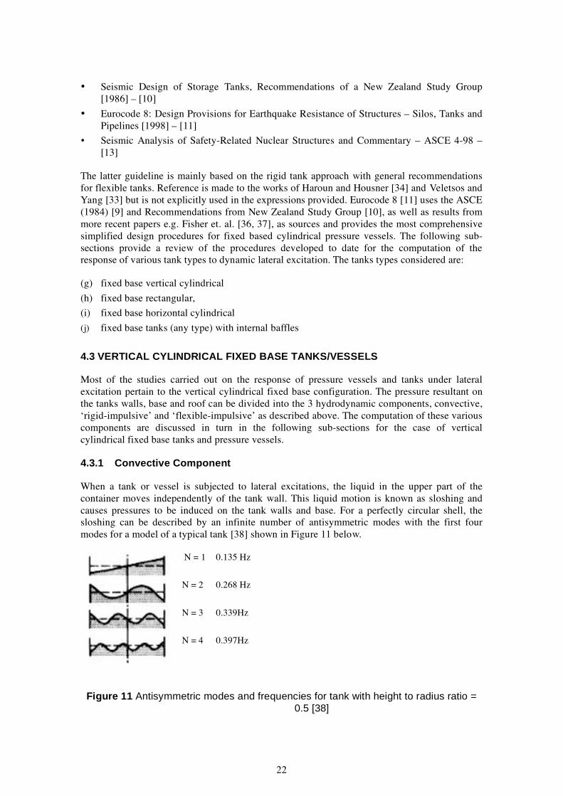
When a tank or vessel is subjected to lateral excitations, the liquid in the upper part of the container moves independently of the tank wall. This liquid motion is known as sloshing and causes pressures to be induced on the tank walls and base. For a perfectly circular shell, the sloshing can be described by an infinite number of antisymmetric modes with the first four modes for a model of a typical tank [38] shown in Figure 11 below.

N = 1 0.135 Hz

N = 2 0.268 Hz

N = 3 0.339Hz

N = 4 0.397Hz

Figure 11 Antisymmetric modes and frequencies for tank with height to radius ratio =

0.5 [38]

22

Symmetrical modes of vibration about the vertical axis are also possible although in general, such modes are not excited by earthquake motions. The frequencies associated with the sloshing modes are usually low (fundamental frequencies usually in the range 0.1 - 0.2 Hz) and for a given mode vary with the tank dimensions and are generally independent of liquid height except for very shallow depths. The jth sloshing frequency in Hertz is given by

1 g � H � f = � tanh � j � (5) j j

2� R � R �

where g is the acceleration due to gravity, R is the tank/vessel radius, H is height of fluid in tank and j are the zeros of the first derivative of the Bessel function of the first kind and first order and values of j for the first four modes are given by

1 = 1.841 2 = 5.331 3 = 8.536 4 = 11.706 (6)

The hydrodynamic pressure induced by the sloshing modes is given by [11]

� r � � z � J1 �� � cosh �� n �

2R � R � R � n

pc = � l � ( ) J ( ) � H � cos � S (7)

2 nn =1 � n -1 1 � n cosh �� n �

� R

where l is the density of the fluid, r, � and z are the radial, circumferential and vertical coordinates respectively, J1 is Bessel function of first order and Sn is the acceleration corresponding to the nth sloshing frequency. The convective pressure varies as a cosine function in the circumferential direction. Generally, only the fundamental sloshing mode is accounted for in the computation of convective pressures as the higher sloshing modes have low mass participations and consequently low associated pressures as shown in Figure 12 (reproduced from reference 11).

Figure 12 Variation of first two modes sloshing pressures along height and for various

height to radius ratios

23

Figure 13 Variation of first two sloshing frequencies with H/R ratio

The convective pressure is a maximum at the top of the tank and decreases to negligible values for tall, slender tanks (H/R � 3) but maintain quite high values for squat tanks. The contribution of the second mode is observed to be negligible. Figure 13 shows that the sloshing frequencies ( is frequency in rad/sec) are nearly independent of the height to radius ratio for values of H/R greater than 1.0.

The maximum convective pressure, accounting for the fundamental sloshing mode only, occurs at z = H (datum at base of tank) and r = R and can be expressed as

p = 0.837 � l S R 1 cos � (8) c max

where S1 is the maximum spectral acceleration value determined from a response spectrum of the particular ground motion at the fundamental sloshing frequency and damping value. Usually, the damping in the sloshing modes is very low (around 0.5%) and is generally assumed to be zero (for light viscosity liquids and tanks with no internal baffles [37]) for design purposes as this leads to a conservative estimate of the pressures.

The convective component is, in general, assumed to be decoupled from the effects of tank wall flexibility [33, 34] so that the same expressions can be used for both rigid and flexible tanks for computing the pressure contributions from sloshing. In ASCE-1984 [9], based primarily on the work of Veletsos [31] and Veletsos and Yang [33], it is argued that

• Convective effects arise from sloshing motion of liquid whereas impulsive effects are caused by the lateral motion of the tank and participating liquid. Consequently, those two effects exhibit only a weak coupling. The tank flexibility alters the lateral motion of the tank wall so that only the impulsive component is significantly affected.

• There exists a wide frequency gap between motions associated with convective and impulsive effects. This further weakens the coupling between the two components and further reduces the sensitivity of one component to changes in the other.

These arguments were basically used to justify the assumption that the wall flexibility does not affect the convective component. This was confirmed by further studies by Haroun and Housner [34].

4.3.2 Rigid Impulsive Component

For a tank or vessel under lateral excitations, the liquid in the lower part of the container tend to move in unison with the tank/vessel and is subject to the maximum ground acceleration. The rigid impulsive pressure component is given in Eurocode 8 [11] as

x (t) (9) p = Ci � H cos � && i l m

where Ci is dependent on the dimensionless parameter z/H and the height to radius ratio and x (t) is the maximum ground acceleration. The variation of Ci (normalised with respect to the &&

m

value at z = 0) along the height of the tank is shown in Figure 14. It is observed that the rigid impulsive pressure decreases from the base of the tank to the top. For tall and slender tanks, the coefficient assumes high values up to significant tank heights.

24

Explicit expressions for the coefficient Ci is provided in Eurocode 8 [11] and result from solution of the momentum equations subject to the assumptions and boundary conditions described in section 4.2. The solution is given in terms of a series expansion as follows:

� (-1)n � �

( C � � ) = i , � ( cos � � I ) 1 �� n �� (10)

I� (� / � � 2 n � �

�)n = 0 1 n n

2n + 1 H r z ,where � = � � = , � = a nd � = . I1and I� denote the modified Bessel function of the n 1

2 R R H

first kind and its derivative. A simplified approximation more amenable to design calculations is

reported by Tedesco et. al. [35] and was first proposed by Housner [28] and used in TID-7024

[29]. The impulsive pressure component in this particular case is given by

Ci (z)/Ci (0)

Figure 14 Variation of Coefficient Ci (z) Along Tank Height For Various Tank Height to

Radius Ratios [9]

2� � 3 �� z 1 � z �&& p = � x H ��1 - � - �1- � tanh 3 �� cos � (11) i l m � �� H 2 � H � R H �

� ��

25

where the symbols have been previously defined. In the above expression, the impulsive pressure is given at the wall of the container so that the radial variation is not contained. The circumferential variation of the rigid impulsive pressure component is a cosine function similar to the convective pressure variation. In the radial direction, the variation is generally non linear

for tanks with low height to radius ratios but tend to a linear distribution for slender tanks as shown in Figure 15 [9].

Figure 15 Radial Variation of Rigid Impulsive Pressure Component For Tanks of Various Height to Radius Ratios [11]

4.3.3 Flexible Impulsive Component

The flexibility of the tank/vessel wall leads to an interaction between the fluid motion and the deformation of the wall. The impulsive pressure due to the coupled tank-fluid vibration usually lies in the high frequency range and results from the contribution of an infinite number of tank-liquid modes. Expressions for the flexible impulsive pressure component have been proposed by various researchers (Haroun & Housner [34]; Veletsos & Yang [33]; Tedesco et. al [35]; Fischer et. al [36]) and are reported in the various codes of practice (Eurocode 8 [11]; ASCE-1984 (9); NZSEE [10]).

The derivation of the expression is, in general, based on the assumption that only the first circumferential m = 1 mode contributes significantly to the pressure. Fischer et. al. [36] reports that this assumption is valid since

26

� �

� �

� �

� �

• Modes with m � 1 do not contribute to the overturning moment which leads to the most common failure mode for tanks and

• Higher order m = 1 modes have low participating mode factors.

The tank-fluid system is considered as a single degree of freedom system vibrating in an assumed configuration. Fischer et. al. [36] proposed the following expression for computing the flexible-impulsive component:

( ) 1 µ � I � j�� � j�� 1 ( )cos� (12) ( )jµ

��

��

R 2 f d= � � �p fin g cos�l µj I�1 2 2

j � 0

where � = x/H0, µj = (j�)/(2�), � = H0/R, I�1 = (j = 1, 3, 5,….). The symbols used in the dI d / �1 j

expression are defined as follows:

pfin flexible-impulsive pressure component normalised to an excitation of 1g

H0 tank height

x axial coordinate

) ( f �f(�) amplitude of vibration mode with max =1

A similar expression is used in Eurocode 8 [11]. The determination of the flexible-impulsive component requires an iterative procedure. It starts with an assumed mode shape from which an updated effective mass of the tank can be calculated. The next iterative step involves computing the new mode shape based on the updated value of the tank mass. This procedure is repeated until convergence is achieved.

An expression for the flexible impulsive component more amenable to design was proposed by Tedesco et. al. [35] is given by

2� �� z � z ( && S x - )H 1 cos � (13) � �� �p fi = �- � �l a m� H � H � �� � 0 �

where H0 is the height of the tank, (z/H0) is an assumed deflection configuration and Sa is the spectral acceleration corresponding to the natural frequency of the flexible tank-liquid system vibrating in the assumed configuration. Based on a statistical analysis of the mode shapes associated with free vibration of tank-liquid systems, Tedesco et. al. [35] have proposed simplified approximations to the deflection configuration parameter for tanks filled and half-filled with fluid.

The approach adopted by Veletsos and Yang [33] was to use a single expression to compute the total impulsive (both rigid and impulsive) pressure and is given by

pit =C� � l A H ( )cos � (14) ti 0

where pit is the total impulsive pressure, is the counterpart of Ci in the expression for rigid C�i impulsive pressure component and A0 (t) is the pseudo-acceleration evaluated for the natural frequency and damping ratio of the flexible tank-fluid system. In addition to the height to radius

27

ratio and z/H, the coefficient also depends on the assumed deflection configuration and the C�i ratio of the mass of the tank to the mass of the fluid.

The deflection configuration of the tank-liquid system depends on the geometry of the container, the material properties of the tank/vessel, the depth of the liquid and the boundary conditions at the top and bottom of the tank/vessel. Veletsos and Yang [33] summarised the deflection characteristics of an empty tank based on the H/R ratio as follows:

• For large values of H/R, the tank deflects in a cantilever flexural beam mode with practically no distortion of the cross-section

• For smaller values of H/R, the deflection shape is as a cantilever shear beam with no distortion of the cross-section

• For yet smaller values of H/R, the deflection configuration of the tank can be represented as a series of ovalling modes and

• For extremely small values of H/R, the tank/vessel wall behaves as a series of independent cantilever flexural strips.

The vibrational characteristics of the tank-liquid system are similar to those of the empty tank. Kana [38] reports that flexural modes are more important in tanks with H/R > 1 while more than one ovalling mode may be important in tanks of all sizes.

Expressions for the fundamental natural frequency of the flexible impulsive mode of vibration have been proposed by various researchers based on different approaches including finite element methods and the Rayleigh-Ritz procedure. Rammerstorfer et. al. [39] provide a comparison between the various expressions and conclude that, in general, they exhibit good agreement. The approximation provided in Eurocode 8 [11] is as follows:

1 s E 3 1 2f = g ( )= 0.01675 � - 0.15 � + 0.46 (15) � s g R 2 ( ) � H�

where E is the Young’s Modulus of the material of the tank/vessel, s is the thickness at 1/3 height and is the density of the liquid.

In the various procedures developed for computing the flexible impulsive response, an important assumption is that the cross section of the tank is truly circular. The effect of out-of-roundness and other imperfections would be to excite modes involving more than a single sine wave in the circumferential direction, which may significantly affect the response of the system [39].

In summary, the main difference between the response of a rigid and flexible tank pertains to the nature of the acceleration component. For a rigid tank, the response is proportional to the maximum ground acceleration whereas for a flexible tank, the response is governed by the spectral acceleration corresponding to the fundamental frequency of the tank-liquid vibration and associated damping ratio. The flexible impulsive frequencies usually lie in the range 2 – 20 Hz. Within this region, the spectral acceleration, for a given damping ratio, is typically greater than the maximum ground acceleration. In general, the damping in the flexible impulsive mode is assumed to be approximately 2% (Rammerstorfer et. al. [39]).

28

4.4 RECTANGULAR FIXED BASE TANKS

Results for rectangular tanks have originally been proposed by Housner [28] based on the same structure and fluid assumptions as for a rigid vertical cylindrical fixed base tank. The response of the rigid tank is again considered to be made up of a convective part and a rigid impulsive part.

4.4.1 Convective Component

The convective pressure component results from the contribution of an infinite number of sloshing modes. However, as for the case of a cylindrical tank, the dominant contribution arises from the first sloshing mode. The fundamental sloshing frequency for rectangular tanks can be expressed as [11]:

� � � H � tanh � �

1 2 � 2 L �f1 = (16)

2 � g L

where g is the acceleration due to gravity and L is the half-width of the tank in the direction of the excitation. Plots of the first two sloshing frequencies (dimensionless period in this case) for

both cylindrical and rectangular tanks are shown in Figure 16.

29

Figure 16 Variation of First and Second Mode Sloshing Periods For Cylindrical and

Rectangular Tanks With Height to Radius Ratio (Cylindrical) or Height to

Half Width Ratio (Rectangular)

The slosh frequencies pertaining to the rectangular tanks are lower than for the cylindrical case. In both cases, the frequencies tend to become independent of the height to half-width (rectangular tanks) or height to radius (cylindrical tanks) ratios.

The convective pressure on the tank/vessel wall, perpendicular to the direction of motion, from the fundamental sloshing mode is given by [11]:

p = q � S L 1 (17) c 1

where q1 is a dimensionless convective pressure corresponding to the first sloshing mode (Figure 17) and S1 is the spectral acceleration corresponding to a response spectrum for the ground motion under consideration at the fundamental sloshing frequency and damping ratio.

Figure 17 Dimensionless Convective Pressure For First Sloshing Mode on

Rectangular Tank Walls

The variation of the dimensionless convective pressure on the rectangular tank walls is similar to that of the convective pressure distribution for cylindrical tanks (Figure 12). The same

30

variation is observed with H/R whereby the convective effects become more pronounced at the base of the tank as H/R decreases i.e. for squat tanks.

Again, as for the cylindrical tank, the damping ratio in the sloshing modes of vibration is usually negligible and is assumed to be zero for conservative results. Also, the wall flexibility does not affect the convective component so that the same expressions can be used for both rigid and flexible tanks.

4.4.2 Rigid Impulsive Component

The approach for determining the rigid impulsive component is similar to that for cylindrical tanks and the pressure component in this case is given by [11]:

0 z && pi = q ( )� x L (18) m

where the function q0 (z) is shown in Figure 18. All other symbols have been previously defined. The variation is similar to that of the rigid impulsive pressure coefficient for cylindrical tanks.

Figure 18 Dimensionless Impulsive Pressures on Rectangular Tank Wall Perpendicular to Direction of Excitation

31

4.4.3 Flexible Impulsive Component

The wall tank flexibility results in an interaction between the deformation of the wall and the motion of the liquid. In the case of rectangular tanks, however, no closed form expression for determining the magnitude of the flexible impulsive component is available. Solutions can, however, be obtained through linear finite element dynamic analysis.

An approximation reported in Eurocode 8 [11] is to use the same expression as for the rigid rectangular tank with the spectral acceleration Sfi replacing the maximum ground acceleration. The spectral acceleration is evaluated at the fundamental frequency and damping ratio of the tank-liquid mode based on the response spectrum of the excitation under consideration.

The fundamental frequency of the tank-liquid mode can be approximated as [11]:

1 gf = (19)

2 � d f

where g is the acceleration due to gravity, df is the deflection of the wall on the vertical centreline and at the height of the impulsive mass, when the wall is loaded by a uniform load in the direction of ground motion and of magnitude mi g / 4 B H, mi is the impulsive mass and 2B is the tank width perpendicular to the direction of loading.

4.5 FIXED BASE HORIZONTAL CIRCULAR CYLINDRICAL TANKS/VESSELS

For the case of horizontal circular cylindrical tanks, the response is further complicated by

• Cross sectional curvature and

• Possible significant length differences longitudinally compared to laterally.

The slosh configurations would differ along the tank axes so that both the longitudinal and lateral components of the excitation must be taken into account.

Few studies have been carried out to investigate the response of horizontal circular cylindrical tanks. Experimental studies on the slosh response are reported by Kana [38] and compared to predictions based on expressions for rectangular tanks. These studies showed that non-linearities have a significant effect on the response of horizontal circular cylindrical tanks.

For the impulsive component, Eurocode 8 [11] recommends that the pressures in both the longitudinal and lateral directions be computed from rectangular tank solutions by assuming an equal dimension at the liquid level and in the direction of excitation and at a depth required to give equal liquid volume. The approximation is considered valid for the range 0.5 � H/R � 1.6. For values greater than 1.6, the tank should be assumed to be full.

An approximate expression for determining the rigid-impulsive response is provided in Eurocode 8 [11] for partially filled tanks and for a seismic excitation perpendicular to the length of the tank and is given by

p ( )= q ( )� A R ( ) (20)ö ö ti 0 g

where R is the radius of the tank, Ag (t) is the input acceleration at time t, and the pressure function q0 (�) is given by

32

n�1 -1H � ( )

q0 (� ) = 2

2nö sin (21)� � n =1 ( ) -12n

The function is plotted in Figure 19. No closed form expressions have been proposed for determining the convective component of response. However, the sloshing frequency in the first mode can be obtained from Figure 20.

Figure 19 Rigid-Impulsive Pressure Variation on Horizontal Cylinder (H = R) Subjected

To Transverse Excitation [11]

33

Figure 20 Dimensionless First Convective Mode Frequency for Rigid Tanks of Various

Shapes [11] 4.6 TANKS WITH INTERNAL BAFFLES

The design of tanks of various types with internal baffles is addressed in the aerospace monographs [40, 41] and is mainly concerned with slosh suppression. Baffles increase the effective fluid damping thereby reducing the duration of free oscillations and magnitude of forced oscillations. The variation of the effective damping ratio with baffle location for rigid ring baffles in a circular cylindrical tank is shown in Figure 21.

�1 is the maximum sloshing wave height measured from the quiescent liquid surface at tank wall. The results are based on the assumption that the baffle remains in the fluid during sloshing. It is observed that

• For a fixed baffle location, the effective damping ratio increases with increasing baffle size i.e. as a0/a decreases and

• For a fixed baffle size, the effective damping ratio increases as the baffle location moves up along the tank height.

34

Figure 21 Variation of Effective Damping Ratio With Baffle Location

The latter observation can be readily explained by the fact that the sloshing effects are more prominent near the top of the liquid surface so that the effectiveness of the baffles in suppressing the sloshing motion would be more evident nearer the top of the fluid surface. For a series of ring baffles, reference 41 suggests that the combined damping ratio can be obtained by adding the contribution of each ring. This approximation has, however, not been thoroughly verified. It is noted that the baffles in this particular case are rigid and that flexible baffles may provide more damping than rigid ones.

In addition to increasing the effective damping ratio, the effect of the baffles is also to reduce the masses associated with sloshing and increase the sloshing frequencies. Similar effect is achieved by compartmentalising the tank i.e. subdividing it into smaller regions and also by internal components within the tank. Ma et. al. [42] carried out a finite element analysis on a reactor tank with internal components and found that the presence of internals (e.g. pumps) can significantly alter the dynamic characteristics of the sloshing motion. Notably, the fundamental frequency is considerably increased with the sloshing wave height reduced. The hydrodynamic pressure was also found to increase.

This can be explained as follows. In the low frequency region (usually <5Hz) of the spectrum (earthquake, blast, ship impact), the acceleration increases sharply as the frequency increases. The presence of baffles increases the natural sloshing frequencies so that the associated accelerations are higher. However, the sloshing masses are reduced so that the increase in pressure due to the higher accelerations is counterbalanced by the reduction in mass. In the above case, the effect of higher acceleration is more dominant than the decrease in sloshing masses.

4.7 ROCKING RESPONSE OF VESSELS/TANKS

Vessels and tanks on topsides will also be subject to rocking motions because of the flexibility of the supporting deck even under purely translational free-field ground excitation of the platform or lateral excitation from ship impact and blast. The rocking response of cylindrical vertical tanks has been investigated by Haroun and Housner [43] and Haroun and Ellaithy [44]. Based on the same assumptions as for purely lateral motion, the latter proposed a spring-mass

35

model for determining the rocking response. Explicit values are provided for the various parameters characterising the system based on the additional assumption that the deformed shape of the tank (for flexible tanks) is taken as sin (�z/2H) where z is the vertical coordinate and H is the height of the liquid in the tank.

Veletsos and Tang [45] considered the same problem and proposed approximate expressions similar to that for tanks under purely lateral excitation. By decomposing the rocking motion of the tank into a rotation of wall with no base rotation and rotation of base with no wall rotation, it was shown that the impulsive component of wall pressure for tall tanks is dominated by rocking action of the wall and for broad tanks, it is dominated by the rocking action of the base. A similar conclusion was postulated for the pressures acting on the base.

The above studies pertained to upright cylindrical tanks only and results for tanks of other configurations are not available.

4.8 COMBINATION OF PRESSURES AND RESULTANT STRESSES

Two different procedures are widely used in the literature for combination of the impulsive and convective components namely a direct numerical addition of the absolute maxima and the SRSS rule. The direct summation of the absolute maxima clearly results in a conservative result as it is based on the assumptions that

• The maximum values of the convective acceleration and the flexible impulsive pseudo-acceleration occur simultaneously with the maximum ground acceleration and

• Maximum positive and maximum negative values of the convective acceleration and the flexible impulsive pseudo-acceleration are equally likely

In general, the convective fluid pressure does not occur simultaneously with the 2 impulsive fluid parts. An alternative superposition rule is based on the square-root-of-sum-of-squares (SRSS) method. Fischer et. al. [36] proposed three sets of different SRSS superposition rules based on the natural frequency of the flexible impulsive mode of vibration. A more general SRSS rule proposed by Fischer et. al. [36] and is given by

2 2 p = ( ) (p + pfi ) (22) pmax c + ri

where pc is the convective pressure and pri, pfi are the rigid impulsive and flexible impulsive pressure components respectively.

The total pressure on the tank wall should include both the hydrodynamic pressure and the hydrostatic pressure. The tank forces and stresses can then be calculated based on an appropriate shell theory. In general, only the maximum values of the circumferential, shearing and axial stresses in the tank walls are required. Following the Veletsos and Yang [33] procedure, as reported in ASCE-1984 [9], the maximum values of the stresses can be determined from:

P R maxMaximum Hoop or Circumferential Stress: ( ) = (23) � � max H

Maximum Shear Stress: � = 2 Q max =

1 Q max (24) max A � H R s

36

( ) = M max R 1 M maxMaximum Axial Stress: � = (25) z max

I � R 2 H

where Qmax is the maximum base shear, Mmax is the maximum overturning moment and I is the moment of inertia of the tank wall about a horizontal centroidal axis. The maximum base shear and overturning moment can be evaluated from expressions proposed by Veletsos and Yang [33] amongst others. Simplified approximations have been proposed by Malhotra et. al. [46] whereby the base shear and overturning moment are calculated from:

fM =m i h i S ( )+m h S ( ) (26) e f imp c c e con

where mi, mc are the impulsive and convective masses respectively, hi, hc are the heights of the centroids of the impulsive and convective masses respectively, Se (fimp) is the spectral acceleration from a response spectrum of appropriate damping ratio at the tank-liquid frequency and Se (fcon) is the spectral acceleration from a response spectrum at the sloshing frequency. The masses and heights can be determined from figures presented in the paper.

Balendra et. al. [47] provides a good discussion of the stress resultants in flexible cylindrical tanks and reports that for broad and shallow tanks, the circumferential stress is the largest among all the membrane stress resultants. As the height-to-radius (H/R) ratio increases, the membrane shear stress becomes dominant and for tall and slender tanks (large H/R ratios), the axial stress predominates. It is pointed out, however, that the design criterion may not be set by the value of the maximum stress. This is because the hoop stress is tensile while the axial stress may be compressive which can result in buckling at lower stresses.

4.9 SUMMARY OF DYNAMIC RESPONSE OF VESSELS/TANKS UNDER LATERAL

EXCITATION

• The response of a tank/vessel under lateral excitation can be split into three hydrodynamic components termed convective or sloshing component, rigid-impulsive component and flexible-impulsive component.

• The frequencies associated with the sloshing are usually quite low (fundamental frequency between 0.1 – 0.2 Hz). Generally, only the first sloshing mode is considered for design purposes. However, while this assumption is accurate for determination of pressures, it may lead to unconservative results for the displacement of the fluid where higher mode effects can be important.

• The rigid-impulsive component is due to the rigid body motion of the fluid and is subjected to the maximum ground acceleration. The flexible-impulsive component accounts for the flexibility of the tank/vessel and is subjected to the acceleration pertaining to the relevant modes of vibration of the tank-fluid system.

• The damping associated with the sloshing modes is usually quite low (approximately 0.5%). However, it should be noted that for higher viscosity fluids and tanks/vessels with internal baffles, the damping value is higher. For the impulsive components, the damping ratio is generally assumed to be approximately 2%.

• S implif ied procedures have been developed in the literature f or computing the response of

f ixed base vertical cylindrical tanks/vessels. For other tanks types (rectangular, horizontal

cylindrical), resort must be made to linear/non-linear f inite element dynamic analyses as no

simple solutions f or all the hydrodynamic components are available.

37

38

5 CONCLUSIONS

A state-of-the-art review was carried out to assess existing analytical methodologies and simplified models with respect to the modelling of tanks/vessels on offshore platforms. The findings of the review can be summarised as follows:

• 3 different methods exist for analysis of such systems namely simplified uncoupled analysis, uncoupled analysis using deck response spectra or time histories and coupled analysis. The applicability of the methods depends on whether the tank/vessel can be classified as rigid or flexible.

• For rigid vessels/tanks, a simplified uncoupled analysis is recommended. In the case of flexible vessels/tanks where the mass of the tank/vessel is not significant compared to that of the supporting structure and where static constraints do not lead to redistribution of stresses, an uncoupled analysis using deck response spectra of time histories can be used. For tanks/vessels where there is significant interaction (close frequencies of vibration) between the tank/vessel and the supporting structure, a coupled analysis should be used.

• The input loading is important not only in terms of the magnitude of the excitation but also with regard to its frequency content. Different excitations such as blast, earthquake and ship impact have different frequency contents. In general, the earthquake excitation is a low frequency excitation whereas the blast and ship impact loadings can be described as high frequency excitations.

• Simplified models (spring-mass systems) and expressions exist for the representation of vertical cylindrical tanks. The response of such tanks/vessels to dynamic excitation is governed by 3 hydrodynamic components namely the rigid-impulsive component (part of fluid moving synchronously with tank), the flexible-impulsive component (coupled tank-fluid motion) and the sloshing component. The relative contribution of these components to the total response depends on the aspect ratio of the tank/vessel, level of fluid and the magnitude and frequency content of the input excitation.

• Similar simplified models also exist for rectangular tanks, which are fully supported along the bottom. Expressions exist in the literature for computing the contributions from the rigid-impulsive and sloshing components. However, no such expressions exist for the flexible-impulsive component. In the latter case, the response is approximated by assuming that the pressure contribution varies similarly to the rigid-impulsive component except that the ground acceleration is replaced by the spectral acceleration at the flexible-impulsive frequency.

• No simplified models or expressions exist for horizontal cylindrical tanks with flat or dished ends (approximate method is provided in Eurocode 8 [11] based on the rectangular tank case). Review of tanks/vessels on offshore platforms has shown that the latter configuration (i.e. horizontal cylindrical tanks with semi-ellipsoidal heads) is the most common type of production vessels. Generally, these vessels are supported on saddle supports, which are bolted to the deck structure.

39

6 REFERENCES

1. Cullen, The Honourable Lord, ‘Public Enquiry into the Piper Alpha Disaster’, HMSO, 1990

2. Health and Safety Executive, ‘A guide to the Offshore Installations (Safety Case) Regulations’, HMSO, 1992

3. Eatec Ltd, ‘Blast and Shock Induced Vibrations in Offshore Jacket Installations’, Health and Safety Executive Report OTH 94 430, 1994

4. ISO/CD 19901-3, ‘Petroleum and natural gas industries – Specific requirements for offshore structures – Part 3: Topsides structure’, 2001

5. API Recommended Practice 2A-WSD, ‘Recommended Practice for Planning, Designing and Constructing Fixed Offshore Platforms – Working Stress Design’, 2000

6. NORSOK Standard N-003, ‘Action and Action Effects’, 1998

7. NORSOK Standard N-004, ‘Design of Steel Structures’, 1998, Rev 1

8. ISO/CD 19902, ‘ Petroleum and Natural Gas Industries – Fixed Steel Offshore Structures’, 2001

9. American Society of Civil Engineers (ASCE), ‘Guidelines for the Seismic Design of Oil and Gas Pipeline Systems’, 1984

10. Priestley, M.J.N (Ed.), ‘Seismic Design of Storage Tanks’, Recommendations of a study group of the New Zealand National Society for Earthquake Engineering, 1986

11. European Committee for Standardisation, ‘Eurocode 8: Design provisions for earthquake resistance of structures – Part 4: Silos, tanks and pipelines’, 1998

12. Department of Energy, ‘Offshore Installations: Guidance on design, construction and certification’, 4th Edition, HMSO, 1990

13. ASCE, ‘Seismic Analysis of Safety-Related Nuclear Structures and Commentary’, 1998

14. Committee on Nuclear Structures and Materials of Structural Division of ASCE, ‘Structural Analysis and Design of Nuclear Plant Facilities’, 1980

15. EQE International Ltd, ‘Development of walkdown procedures and pilot study for the assessment of topsides equipment subject to blast induced vibrations’, Health and Safety Executive Report OTH 93 415, 1995

16. Kost, G., Sharpe, R.L., ‘Seismic Resistant of Piping, Equipment and Appurtenances for Offshore Structures’, Offshore Technology Conference, OTC 2750, 1977

17. Craig, M.J.K., Dolan, D.K., Turner, J.W., ‘API RP-2A 20th Edition Update: Seismic Topsides Design and Assessment Guidelines’, OTC 7156, 1993

18. Bea, R., Bowen, C., ‘Simplified Earthquake Floor Response Spectra for Equipment on Offshore Platforms’,

19. Biggs, J.M., Roesset, J.M., ‘Seismic Analysis of Equipment Mounted on a Massive Structure’, Siemic Design of Nuclear Power Plants, R J Hansen (Ed.), 1970

20. Clough and Penzien, ‘Dynamics of Structures’

21. Smith, C.E., ‘Response of a steel-jacket Platform subject to Measured Seafloor Seismic Ground Motions’, OTC 8110, 1996

40

22. Renwick, P., Norman, T., ‘Fire and Blast Engineering in the Offshore Oil and Gas Industry – Developments since Piper Alpha’, ERA

23. Walker, D.G., Ramsden, M., Bruce, R.L., ‘Blast Induced Vibrations on Topsides’, ERA

24. Donegan, E.N., Brown-Earl, J., Wright, ‘Appraisal of Accidental Impact loadings on steel piled North Sea’, OTC 4193, 1982

25. Petersen, M.J., Pedersen, P.J., ‘Collisions between ships and offshore platforms’, OTC 4134, 1981

26. Blok, J.J., Brozius, L.H., Dekker, J.N., ‘The Impact Loads of Ships Colliding with Fixed Structures’, OTC 4469, 1983

27. Litton, R.W., Puskar, F.J., ‘Ship Collision Analysis for the Kawasaki Island Steel Platforms’, OTC 7141, Vol 2, 1993

28. Housner, G.W., ‘Dynamic Pressures on Accelerated Fluid Containers’, Bulletin of the Seismological Society of America, Vol 47, Jan 1957

29. US Atomic Energy Commission, Nuclear Reactors and Earthquakes, TID-7024, Office of Technical Service, Washington DC, 1963

30. Epstein, H.I., ‘Seismic Design of Liquid Storage Tanks’, Journal of the Structural Division, ASCE, Vol. 102, No. ST9, 1976

31. Veletsos, A.S, ‘Seismic Effects in Flexible liquid storage tanks’, Proceedings of International Association for Earthquake Engineering, 1974

32. Kana, D.D., Dodge, F.T., ‘Design support modelling of liquid slosh in storage tanks subject to seismic excitation’, Proceedings ASCE conference on Structural Design of Nuclear Plant Facilities, 1975

33. Veletsos, A.S., Yang, J.Y., ‘Earthquake Response of Liquid storage Tanks’, Advances in Civil Engineering through Engineering Mechanics, ASCE, 1977

34. Haroun, M.A., Housner, G.W., ‘Seismic Design of Liquid Storage Tanks’, ASCE, Vol 107, 1981

35. Tedesco, J.W., Landis, D.W., Kostem, C.N., ‘Seismic Analysis of cylindrical liquid storage tanks’, Computers and Structures, Vol. 32, No 5, 1989

36. Fischer, F.D., Rammerstorfer, F.G., Scharf, K., ‘Earthquake Resistant Design of Anchored and Unanchored Liquid Storage Tanks under 3D Earthquake Excitation’, Structural Dynamics Recent Advances, Schneller G.L. (Ed.), Springer Verlag, 1991

37. Fischer, F.D., Rammerstorfer, F.G., ‘The Stability of Liquid-Filled Cylindrical Shells Under Dynamic Loading’, Buckling of Shells, Proceedings of the State-of-the-Art Colloquium, Springer, Berlin, 1982

38. Kana, D.D., ‘Status and Research Needs for Prediction of Seismic Response in Liquid Containers’, Nuclear Engineering and Design, Vol 69, 1982

39. Rammerstorfer, F.G., Scharf, K., ‘Storage Tanks Under Earthquake Loading’, Applied Mechanics Review, 1990

40. NASA SP-8009, ‘Propellant Slosh Loads’, 1968

41. NASA SP-8031, ‘Slosh Suppression’, 1969

42. Ma, D.C., Gvildys, J., Chang, Y. W., ‘Sloshing Response of Reactor Tank With Internals’, Engineering Mechanics

41

43. Haroun, M.A., Housner, G.W., ‘Dynamic Interaction of Liquid Storage Tanks andFoundation Soil’, Proceedings of Second ASCE/EMD Speciality Conference on DynamicResponse of Structures, Atlanta, Georgia, 1981

44. Haroun, M.A., Ellaithy, H.M., ‘Model for Flexible Tanks Undergoing Rocking’, Journal ofEngineering Mechanics, ASCE, Vol 111, No. 2, 1985

45. Veletsos, A.S., Tang, Y., ‘ Rocking Response of Liquid Storage Tanks’, Journal ofEngineering Mechanics, ASCE, Vol 113, No. 11, 1987

46. Malholtra, P.K., ‘Seismic Analysis of Liquid Storage Steel Tanks’, Structural EngineeringInternational, 1997

47. Balendra, T., Ang, K.K, Paramasivam, P., Lee, S.L., ‘Seismic Design of FlexibleCylindrical Liquid Storage Tanks’, Earthquake Engineering and Structural Dynamics, Vol10, 1982.

42

Health and Safety Executive

Fluid structure interaction effects on and dynamic response of pressure vessels and tanks subjected to dynamic loading Part 2: Determination of sloshing frequencies

The Steel Construction Institute Silwood Park Ascot Berks SL5 7QN

As part of a suite of work looking at fluid interaction effects on (and the dynamic response of ) pressure vessels and tanks subjected to dynamic loading, this report details the findings of work to determine the sloshing frequencies of liquid within a horizontal, cylindrical vessel - the most commonly encountered type of vessel on offshore platforms. Due to the complexity of fluid-structure interaction, it was assumed that the vessel was rigid with flat ends. A series of explicit finite element dynamic analyses were undertaken. A Fourier decomposition of the output force was carried out to provide an insight into the frequency content. The results show good agreement with the codified equation for a rigid rectangular tank.

This report and the work it describes were funded by the Health and Safety Executive (HSE). Its contents, including any opinions and/or conclusions expressed, are those of the authors alone and do not necessarily reflect HSE policy.

HSE Books

© Crown copyright 2007

First published 2007

All rights reserved. No part of this publication may bereproduced, stored in a retrieval system, or transmitted inany form or by any means (electronic, mechanical,photocopying, recording or otherwise) without the priorwritten permission of the copyright owner.

Applications for reproduction should be made in writing to:Licensing Division, Her Majesty’s Stationery Office,St Clements House, 2-16 Colegate, Norwich NR3 1BQor by e-mail to hmsolicensing@cabinet-office.x.gsi.gov.uk

ii

CONTENTS

EXECUTIVE SUMMARY V

1 INTRODUCTION 1 1 .1 BACKGROUND 1 1 .2 OBJECTIVES OF STUDY 2 1 .3 SCOPE OF STUDY 2

2 ASSUMPTIONS AND FE MODELLING 3 2 .1 INTRODUCTION 3 2 .2 VESSEL CONFIGURATION AND ASSUMPTIONS 3 2 .3 FINITE ELEMENT MODELLING 3 2 .4 LOADING 5 2 .5 ESTIMATION OF FIRST SLOSHING FREQUENCY 5

3 RESULTS FOR UN-BAFFLED VESSEL 7 3 .1 INTRODUCTION 7 3 .2 EXCITATION FREQUENCY RANGE AND ANALYSES 7 3 .3 RESULTS AND DISCUSSION 7

4 RESULTS FOR PERFORATED B AFFLED VESSEL 1 7 4 .1 INTRODUCTION 1 7 4 .2 ANALYSIS 1 7 4 .3 RESULTS AND DISCUSSION 1 7

5 CONCLUSIONS 2 1

6 REFERENCES 2 3

iii

iv

EXECUTIVE SUMMARY

This report addresses the determination of sloshing frequencies for a horizontal, cylindrical vessel which is the most commonly encountered type of vessel on offshore platforms. Part 1 of this study reported that there is a lack of guidance for the determination of sloshing frequencies and sloshing masses for vessels of this configuration.

In this study, a series of explicit finite element dynamic analyses were carried out to determine the sloshing frequency for such vessels. Due to the complexity of the fluid-structure interaction, it was assumed that the vessel was rigid with flat ends instead of flexible with semi-ellipsoidal ends. This implies that the fluid response comprises only of the rigid impulsive and sloshing components.

Both an un-baffled vessel and a perforated baffled vessel were considered in this study. The FE models were excited using known cosinusoidal velocity functions and the excitation frequency was varied to cover the typical sloshing frequency range.

A Fourier decomposition of the output force on the vessel was carried out to provide insight into the frequency content of the output force. The results show good agreement with the codified equation for a rigid rectangular tank.

A similar procedure was adopted to determine the sloshing frequencies for a baffled vessel with 3 different fluid fill ratios. It was found that the first sloshing frequency remained unchanged with increasing fluid fill ratio. For the baffled case, there is a significant difference between the analytical sloshing frequency and that from the codified equation. This is attributed to the perforation in the baffles which allow movement of fluid between the compartments.

v

vi

1 INTRODUCTION

1.1 BACKGROUND

The first part of this study provided a state-of-the-art review of the dynamic loading and fluid-structure interaction effects in pressure vessels and tanks on offshore platforms. The most commonly encountered type of vessel is horizontal, cylindrical with semi-ellipsoidal heads. As reported earlier [1], there is, however, a lack of simplified design methods for such vessels.

The response of such vessels under lateral excitation depends not only on the magnitude and frequency content of the loading but also on:

• Aspect ratio of the vessel

• Separation distance between the saddle supports

• Presence of baffles and internal components

• Diameter to thickness ratio of the vessel and

• Ratio of fluid fill height to vessel length i.e. the fluid fill ratio

Determining simplified procedures for the effects of fluid-structure interaction on the vessel under lateral excitation is further complicated by:

• Ellipsoidal ends that provide a stiffening effect,

• Support mechanism that leads to large tank deflections along circumference of vessel particularly at the centre and

• Geometrical asymmetry of vessel which results in different frequencies in the lateral and longitudinal directions.

Currently, the design codes recommend that fluid-structure interaction effects in pressure vessels be accounted for using the approximate expression derived for rectangular tanks. It is recognised that due to the complexity of the problem, simplified procedures for horizontal, cylindrical vessels with semi-ellipsoidal heads cannot be easily derived.

However, it is possible to gain more information by carrying out a limited number of analyses on a simplified tank model namely a rigid vessel with flat ends. In particular, this limited set of analyses will allow the derivation of sloshing frequencies for both un-baffled and baffled configurations. This will provide the structural designer with a starting point to determine whether fluid-structure interaction effects may be important and, if so, whether there is a need for detailed analyses.

1

1.2 OBJECTIVES OF STUDY

This part of the study is concerned with the derivation of sloshing frequencies for a rigid, horizontal, cylindrical tank with flat ends. The main objectives of the study can be summarised as follows:

• Derivation of sloshing frequency for an un-baffled vessel for 1 fluid fill ratio

• Comparison of numerical sloshing frequency for un-baffled vessel against codified equation

• Derivation of sloshing frequencies for baffled vessel for 3 fluid ratios

1.3 SCOPE OF STUDY

To achieve the above objectives, the study is split into several stages as follows:

(a) Carry out a set of linear explicit finite element dynamic analysis of an un-baffled vessel with a fluid fill ratio of 0.2. The excitation will be a cosinusoidal function with a range of frequencies.

(b) Estimate the sloshing frequency for the un-baffled vessel based on the previous analyses.

(c) Compare the sloshing frequency for the un-baffled vessel with codified equation

(d) Carry out 3 sets of linear explicit finite element dynamic analysis of a baffled vessel with fluid fill ratios of 0.15, 0.2 and 0.25. These ratios correspond to commonly encountered fluid fill levels. Again, the excitation will be a cosinusoidal function with a range of frequencies.

(e) Estimate the sloshing frequencies for the 3 fluid fill ratios based on the dynamic analyses.

Chapter 2 provides an overview of the problem and the modelling assumptions for both the un-baffled and baffled vessel. The determination of the sloshing frequency for the un-baffled vessel is described in Chapter 3. Chapter 4 details the analyses and results for the baffled vessel. Finally the findings from this study are described in Chapter 5.

2

2 ASSUMPTIONS AND FE MODELLING

2.1 INTRODUCTION

This chapter provides a description of the assumptions used for this study for the determination of sloshing frequencies for horizontal, cylindrical vessels with flat ends. The finite element models and the dynamic excitation applied to the various models are also described. Finally, the procedure adopted for determining the sloshing frequency is provided.

2.2 VESSEL CONFIGURATION AND ASSUMPTIONS

As mentioned earlier, the vessel considered in this study is horizontal, cylindrical with flat ends. The geometry of the vessel (with baffles – un-baffled vessel has similar geometry) is illustrated in Figure 2.1:

2 m

2.5 m

Perforated Baffles

2 m 2 m 2 m

6 m

Figure 2.1: Geometry of vessel used in sloshing analyses

The chosen geometry for the vessel is based on typical dimensions of vessels found on offshore modules. The following assumptions are made to simplify the model:

• The vessel is assumed to be rigid so that it can be modelled using rigid elements

• The fluid motion is assumed to be linear

The following further simplifications are made for the baffled vessel:

• The perforated baffles are rigid

• The perforated baffles divide the vessel into 3 equal parts

• The perforated area is approximately 20% of the total baffle area

2.3 FINITE ELEMENT MODELLING

The dynamic finite element analyses were carried out using the explicit dynamics software MSC Dytran [2]. The software is well suited to dealing with fluid-structure interaction problems either via a general coupling algorithm or an arbitrary Lagrangian-Eulerian formulation.

3

A description of the latter formulation and of the numerical considerations for explicit dynamics analysis is given in part 3 [3] of this study. The following sections provide a brief description of the finite element models for both the un-baffled and the baffled vessels.

2.3.1 Modelling of Un-baffled Vessel

As reported in the state-of-the-art review in the first part of this study [1], it is well known that the sloshing frequencies generally lie in the range of 0.1 to 0.2 Hz. In order to limit the number of full 3D analyses that need to be carried out to determine the sloshing frequency, a simplified 3D model was used to narrow the sloshing frequency range.

For both the simplified 3D and the full 3D models, a rigid element was used to model the rigid vessel. It is noted that no matter how many elements and properties are used to make up the rigid body, in the solution it is treated as a single element.

The material properties for the vessel structure were as follows:

• Material: Steel

• Density: 7850 kg/m3

• Young’s Modulus: 2.05e11 N/m2

• Poisson’s Ratio: 0.3

• Thickness: 30 mm

MSC Dytran automatically calculates the geometric properties of the rigid body such as themass, the centre of gravity and the moments of inertia.

The fluid fill ratio for the un-baffled case was 0.2 i.e. a water level of 1.2 m. The fluidproperties were as follows:

• Density: 1000 kg/m3

• Bulk Modulus: 2.2e06 N/m2

• Cavitation Pressure: -1.0e05 N/m2

The fluid was modelled using Eulerian solid elements based on an isotropic, non-viscous model.

Simplified 3D Model

In order to narrow the frequency range to be considered for the full 3D analyses, a simplified 3D model was developed. The simplified 3D model was essentially a longitudinal slice along the vessel with 3 elements in the lateral direction.

The model was restrained translationally in the y and z direction and in all 3 directions rotationally. The excitation was applied as a cosinusoidal velocity function in the x-direction (longitudinal) and is described further in section 2.4.

Full 3D Model

The mesh density and boundary conditions for the full 3D model were similar to that for the simplified 3D model. The excitation was, again, applied as a cosinusoidal velocity function in the longitudinal direction as described in section 2.4.

4

2.3.2 Modelling of Baffled Vessel

The baffled vessel configuration is shown in Figure 2.1. As mentioned earlier, the baffles are assumed to be rigid. Due to the perforations in the baffles, it was not possible to use a simplified model as in the un-baffled case. The perforated area was assumed to be 20% of the total baffle area.

The perforations were modelled by numerically removing elements from the baffles. The boundary conditions were the same as that used for the un-baffled case. The loading applied to the model is described in the following section.

2.4 LOADING

The excitations applied to the models were cosinusoidal velocity functions of the form:

(t) v = 2 cos V �f t n

where V is the amplitude of the velocity and fn is the frequency of excitation.

The velocity function was applied to both the rigid element (used to model the vessel structure) and the Eulerian mesh to ensure compatibility at the Lagrangian/Eulerian boundary as per the Arbitrary Lagrangian Eulerian (ALE) formulation.

2.5 ESTIMATION OF FIRST SLOSHING FREQUENCY

The procedure for determining the sloshing frequency is illustrated in the flow-chart shown in Figure 2.2. Essentially, the procedure consists in getting the maximum amplitude of the output force on the rigid element at various excitation frequencies.

A plot of the maximum amplitude against excitation frequency will subsequently allow for an estimation of the first sloshing frequency.

5

VESSEL

FINITE ELEMENT MODEL OF

APPLY LOADING AT

EXCITATION FREQUENCY Fn

RUN ANALYSIS

OUTPUT TIME HISTORY OF

FORCE ON RIGID ELEMENT

FOURIER DECOMPOSITION OF

OUTPUT FORCE

GET PEAK AMPLITUDE OF

FOR CE FOR EXCITATION

FREQUENCY Fn

END OF EXCITATION

FREQUENCY RANGE ?

PLOT PEAK AMPLITUDE

AGAINST EXCITATION

FREQUENCY

NEXT n

ESTIMATE FIRST SLOSHING

FREQUENCY

Figure 2.2: Procedure for estimation of first sloshing frequency

6

3 RESULTS FOR UN-BAFFLED VESSEL

3.1 INTRODUCTION

A set of explicit FE analyses were carried out on the simplified 3D model of the un-baffled vessel within the frequency range 0.025 Hz to 0.30 Hz. The results from these analyses were subsequently used to estimate the first sloshing frequency. Full 3D analyses were also carried out in the region of the estimated sloshing frequency in order to confirm the findings from the simplified 3D analyses.

3.2 EXCITATION FREQUENCY RANGE AND ANALYSES

A total of 18 runs were carried out on the simplified 3D model of the un-baffled vessel covering the frequency range 0.025 Hz to 0.30 Hz. The analyses were run for 3 full cycles of excitation followed by the transient response of the fluid. As mentioned earlier, the excitation was applied in the longitudinal direction and the fluid fill ratio was 0.2.

The time history variation of the force on the rigid element in the longitudinal direction was output at steps of 0.05 seconds. A Fourier decomposition of the time history of the force was subsequently carried out using the software MATHCAD.

3.3 RESULTS AND DISCUSSION

The Fourier decomposition provides a breakdown of the force on the rigid element against frequency. The various Fourier plots for the runs carried out at all the excitation frequencies within the frequency range 0.025 Hz to 0.30 Hz are shown in Appendix 1. The Fourier results for the runs at excitation frequencies 0.025 Hz, 0.05 Hz, 0.10 Hz and 0.25 Hz are reproduced below as Figure 3.1, Figure 3.2, Figure 3.3 and Figure 3.4 respectively.

It is observed that at the lower frequencies (Figures 3.1 to 3.3), two distinct peaks are clearly visible within the frequency range 0 to 1.0 Hz. The first peak occurs at the frequency of the forcing excitation as expected. The second peak occurs at approximately 0.27 Hz and pertains to the first sloshing frequency of the fluid.

Figure 3.1: Fourier decomposition of force on rigid element for simplified 3D model of un-baffled vessel (Excitation Frequency = 0.025 Hz)

7

Figure 3.2: Fourier decomposition of force on rigid element for simplified 3D model of un-baffled vessel (Excitation Frequency = 0.050 Hz)

Figure 3.3: Fourier decomposition of force on rigid element for simplified 3D model of un-baffled vessel (Excitation Frequency = 0.100 Hz)

Figure 3.4: Fourier decomposition of force on rigid element for simplified 3D model of un-baffled vessel (Excitation Frequency = 0.250 Hz)

8

This is clearly observed in the results for the Fourier transform of the force at 0.25 Hz where only a single peak is visible and has a significantly higher magnitude than at the other excitation frequencies.

3 analyses were subsequently carried out on the full 3D model of the un-baffled vessel in order to confirm the above finding. The analyses were performed for excitation frequencies at 0.125 Hz, 0.275 Hz and 0.400 Hz. The results are shown in Figure 3.5, Figure 3.6 and Figure 3.7 respectively.

4 1.5 .10

4 1.297�10

4 1 .10

fForce

5000

52.469 0 0 0.5 1 1.5 2

0 freq 2

Figure 3.5: Fourier decomposition of force on rigid element for full 3D model of un-baffled vessel (Excitation Frequency = 0.125 Hz)

5 1.5 .10

5 1.13�10

5 1 .10

fForce

45 .10

44.798 0 0 0.5 1 1.5 2

0 freq 2

Figure 3.6: Fourier decomposition of force on rigid element for full 3D model of un-baffled vessel (Excitation Frequency = 0.275Hz)

9

4 1.5 .10

4 1.242�10

4 1 .10

fForce

5000

30.612 0 0 0.5 1 1.5 2

0 freq 2

Figure 3.7: Fourier decomposition of force on rigid element for full 3D model of un-baffled vessel (Excitation Frequency = 0.400 Hz)

It is clearly observed that the magnitude of the force is significantly higher at 0.275 Hz than at the other excitation frequencies. Also, only a single peak is observed at 0.275 Hz unlike at the other excitation frequencies where secondary peaks can be noted.

It is also noteworthy to observe that for both Fourier results at 0.125 Hz and 0.400 Hz, a peak can be seen at approximately 0.27 Hz. The full 3D results essentially confirm the finding from the simplified 3D model that the first sloshing frequency for the un-baffled vessel for a fluid fill ratio of 0.2 is approximately 0.27 Hz.

3.3.1 Time History Plots

The time history variation of the output force on the rigid element is shown in Figures 3.8(a) to (d) and Figures 3.9(a) to (d) for excitation frequencies corresponding to 0.125 Hz and 0.275 Hz respectively.

In both cases, the loading was applied for 3 cycles of excitation i.e. for 24 sec in the case of f = 0.125 Hz and for 11 sec in the case of f = 0.275 Hz. The free vibration response was subsequently monitored up to 90 seconds.

The results show that in the case of the vessel under the initial excitation at 0.125Hz, there is a rapid decay in the transient output force. In addition, there is no discernible dominant frequency within the free vibration segments. This is probably due to the fact that the initial forcing function did not excite any of the sloshing frequencies so that the resulting transient motion has low amplitude with no dominant frequency.

In the case of he vessel under the initial excitation of 0.275 Hz, a dominant frequency, corresponding to the first sloshing frequency of the un-baffled vessel, is observed in the transient motion.

These time history plots further confirm the findings in the previous section that the first sloshing frequency of the un-baffled vessel is approximately 0.27 Hz.

10

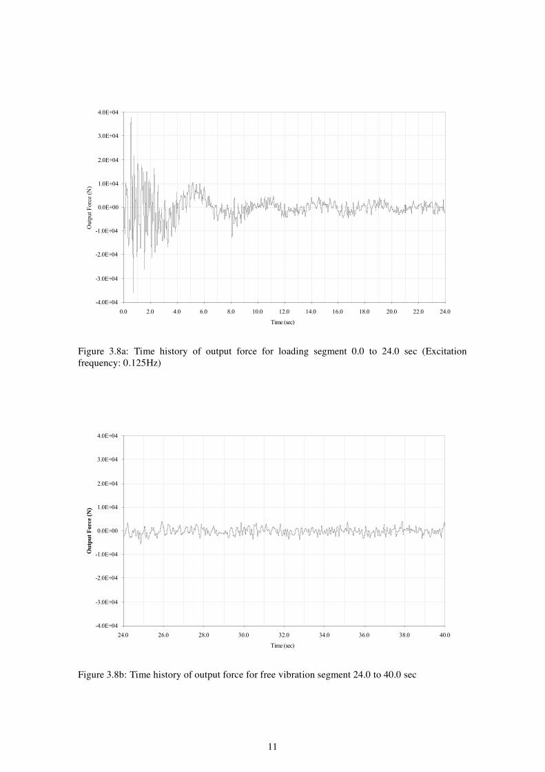
11

-4.0E+04

-3.0E+04

-2.0E+04

-1.0E+04

0.0E+00

1.0E+04

2.0E+04

3.0E+04

4.0E+04

0.0 2.0 4.0 6.0 8.0 10.0 12.0 14.0 16.0 18.0 20.0 22.0 24.0

Time (sec)

Outp

ut

Forc

e(N

)

Figure 3.8a: Time history of output force for loading segment 0.0 to 24.0 sec (Excitationfrequency: 0.125Hz)

-4.0E+04

-3.0E+04

-2.0E+04

-1.0E+04

0.0E+00

1.0E+04

2.0E+04

3.0E+04

4.0E+04

24.0 26.0 28.0 30.0 32.0 34.0 36.0 38.0 40.0

Time (sec)

Outp

ut

Forc

e(N

)

Figure 3.8b: Time history of output force for free vibration segment 24.0 to 40.0 sec

12

-4.0E+04

-3.0E+04

-2.0E+04

-1.0E+04

0.0E+00

1.0E+04

2.0E+04

3.0E+04

4.0E+04

40.0 42.0 44.0 46.0 48.0 50.0 52.0 54.0 56.0 58.0 60.0

Time (sec)

Forc

e(N

)

Figure 3.8c: Time history of output force for free vibration segment 40.0 to 60.0 sec

-4.0E+04

-3.0E+04

-2.0E+04

-1.0E+04

0.0E+00

1.0E+04

2.0E+04

3.0E+04

4.0E+04

60.0 62.5 65.0 67.5 70.0 72.5 75.0 77.5 80.0 82.5 85.0 87.5 90.0

Time (sec)

Outp

ut

Forc

e(N

)

Figure 3.8d: Time history of output force for free vibration segment 60.0 to 90.0 sec

13

-5.0E+04

-4.0E+04

-3.0E+04

-2.0E+04

-1.0E+04

0.0E+00

1.0E+04

2.0E+04

3.0E+04

4.0E+04

5.0E+04

0.0 1.0 2.0 3.0 4.0 5.0 6.0 7.0 8.0 9.0 10.0 11.0

Time (sec)

Outp

ut

Forc

e(N

)

Figure 3.9a: Time history of output force for loading segment 0.0 to 11.0 sec (Excitationfrequency: 0.275Hz)

-5.0E+04

-4.0E+04

-3.0E+04

-2.0E+04

-1.0E+04

0.0E+00

1.0E+04

2.0E+04

3.0E+04

4.0E+04

5.0E+04

11.0 13.0 15.0 17.0 19.0 21.0 23.0 25.0 27.0 29.0

Time (sec)

Outp

ut

Forc

e(N

)

Figure 3.9b: Time history of output force for free vibration segment 11.0 to 30.0 sec

14

-5.0E+04

-4.0E+04

-3.0E+04

-2.0E+04

-1.0E+04

0.0E+00

1.0E+04

2.0E+04

3.0E+04

4.0E+04

5.0E+04

30.0 32.0 34.0 36.0 38.0 40.0 42.0 44.0 46.0 48.0 50.0 52.0 54.0 56.0 58.0 60.0

Time (sec)

Outp

ut

Forc

e(N

)

Figure 3.9c: Time history of output force for free vibration segment 30.0 to 60.0 sec

-5.0E+04

-4.0E+04

-3.0E+04

-2.0E+04

-1.0E+04

0.0E+00

1.0E+04

2.0E+04

3.0E+04

4.0E+04

5.0E+04

60.0 62.0 64.0 66.0 68.0 70.0 72.0 74.0 76.0 78.0 80.0 82.0 84.0 86.0 88.0 90.0

Time (sec)

Outp

ut

Forc

e(N

)

Figure 3.9d: Time history of output force for free vibration segment 60.0 to 90.0 sec

3.3.2 Code comparison

A check was subsequently carried out to compare the above result against that for the codified equation for a rigid rectangular tank. The period of vibration for the first sloshing mode for a rigid rectangular tank [4] is given by:

2� g L T1 =

�1 tanh (� L H )1

�= 2 .where L is the half length of the tank , H is the height of the fluid and �1

� 1st frequency sloshing = Hz 0.27

The correlation between the results of the FE models and the code shows that the methodology adopted to determine the sloshing frequency does provide realistic estimates. It is therefore proposed to use the same approach to determine the first sloshing frequency for vessels with perforated baffles for 3 fluid fill ratios. This is addressed in the next chapter.

15

16

4 RESULTS FOR PERFORATED BAFFLED VESSEL

4.1 INTRODUCTION

As mentioned earlier, the analyses for the perforated baffled vessel were carried out on a full 3D model. No simplifications were possible in this case due to the perforations in the baffles. The perforations were modelled by numerically removing elements from the baffle mesh. The model was, again, based on the Arbitrary Lagrangian Eulerian (ALE) formulation.

4.2 ANALYSIS

3 different fluid fill ratios were considered for the perforated baffled vessel namely 0.15, 0.20 and 0.25 corresponding to a fluid height of 0.9m, 1.2m and 1.5m respectively. 9 analyses were run for each fill ratio within the frequency range 0.125 Hz to 0.90 Hz.

The same methodology, as for the un-baffled case, was adopted to determine the first sloshing frequency namely via Fourier decomposition of the time history of the output force on the rigid element.

4.3 RESULTS AND DISCUSSION

4.3.1 Fluid fill ratio 0.15

The Fourier transforms are shown in Appendix 2. In contrast to the results for the un-baffled case, only a single peak is observed for all the excitation frequencies. This peak occurs at the excitation frequency of the loading applied to the models. The first sloshing frequency can, however, be estimated by the amplitude of the output force at the various excitation frequencies. It is well known that at or close to the sloshing frequency, the output force on the rigid element will be a maximum.

A plot of the peak amplitude (from the Fourier plots) of the output force against excitation frequency is shown in Figure 4.1. It is clearly seen from the result that the first sloshing frequency occurs at 0.60 Hz.

17

0.0E+00

5.0E+04

1.0E+05

1.5E+05

2.0E+05

2.5E+05

3.0E+05

3.5E+05

4.0E+05

4.5E+05 Peak

Amplitu

de

(N)

0.10 0.20 0.30 0.40 0.50 0.60 0.70 0.80 0.90

Frequency (Hz)

Figure 4.1: Variation of Peak Amplitude of Fourier Transform of Force on Rigid Element with Frequency of Excitation (Fluid fill ratio - 0.15)

4.3.2 Fluid fill level 0.20

The Fourier results for the fluid fill ratio of 0.20 are shown in Appendix 3. As in the previous case, only a single peak is observed and this occurs at the excitation frequency. The plot of peak amplitude against excitation frequency is shown in Figure 4.2 and, again, it is seen that the first sloshing frequency occurs at 0.60 Hz.

0.0E+00

1.0E+05

2.0E+05

3.0E+05

4.0E+05

5.0E+05

6.0E+05

7.0E+05

Peak

Amplitu

de

(N)

0.10 0.20 0.30 0.40 0.50 0.60 0.70 0.80 0.90

Frequency (Hz)

Figure 4.2: Variation of Peak Amplitude of Fourier Transform of Force on Rigid Element with Frequency of Excitation (Fluid fill ratio - 0.20)

18

4.3.3 Fluid fill ratio 0.25 Peak

Amplitu

de

(N)

The Fourier results for fluid fill ratio of 0.25 are shown in Appendix 4. The trend is similar to the results for fill ratios of 0.15 and 0.20 with only a single peak at the excitation frequency. The plot of peak amplitude against excitation frequency is shown in Figure 4.3 and it is observed that the first sloshing frequency is 0.60 Hz.

9.0E+05

8.0E+05

7.0E+05

6.0E+05

5.0E+05

4.0E+05

3.0E+05

2.0E+05

1.0E+05

0.0E+00

0.10 0.20 0.30 0.40 0.50 0.60 0.70 0.80 0.90

Frequency (Hz)

Figure 4.3: Variation of Peak Amplitude of Fourier Transform of Force on Rigid Element with Frequency of Excitation (Fluid fill ratio - 0.25)

4.3.4 Comparison of results for fluid fill ratios

Figure 4.4 shows the comparison of the results for the 3 fluid fill ratios. It is observed that:

a) the sloshing frequency for the perforated baffled vessel remains unchanged with increasing fill ratio. This seems to differ somewhat from the results for un-baffled vessels where for fluid fill ratios less than 0.3, the sloshing frequency decreases with decreasing fill ratio.

However, it must be noted that the fill ratios for the baffled and un-baffled vessels are not directly comparable as the baffles compartmentalise the flow to the extent that the fill ratio is actually higher than that for an un-baffled vessel.

It is difficult to assign an accurate value to the fill ratio for the baffled vessel due to the perforations in the baffles which allow fluid to move between the different compartments. However, a simple estimate can be obtained by dividing the fluid height by the length between the baffles. As such, the fluid fill ratios for the baffled vessel correspond to 0.45, 0.60 and 0.75 for the un-baffled vessel.

b) The peak amplitude of the output force increases with increasing fill ratio. For a rigid vessel, the output force on the vessel comprises of the sloshing component and the

19

rigid-impulsive component. The rigid-impulsive component will increase due to the Peak

Amplitu

de

(N)

increased mass of fluid with increasing fill ratios.

c) The peak amplitude for the perforated baffled vessel is higher that that for the un-baffled vessel. This relates to the fact that the increased mass (due to the baffles) leads to higher forces on the vessel.

d) Applying the formula for the rigid rectangular vessel gives a first sloshing frequency of 0.38 for the baffled vessel with fluid height of 1.2m i.e. approximately 0.60 fluid fill ratio. The significant difference between the sloshing frequencies may be due to the perforations in the baffles which allow movement of fluid between the compartments.

9.0E+05

8.0E+05

7.0E+05

6.0E+05

5.0E+05

4.0E+05

3.0E+05

2.0E+05

1.0E+05

0.0E+00

Fluid Fill Ratio 0.15

Fluid Fill Ratio 0.20

Fluid Fill Ratio 0.25

0.10 0.20 0.30 0.40 0.50 0.60 0.70 0.80 0.90

Frequency (Hz)

Figure 4.4: Comparison of results for 3 fluid fill ratios

20

5 CONCLUSIONS

This study has described a procedure for determining the first sloshing frequency for both un-baffled and baffled horizontal, cylindrical, rigid vessels with flat ends. The procedure can be summarised as follows:

a) apply known forcing excitations to a finite element model of the rigid vessel

b) output the force on the rigid element

c) carry out a Fourier transformation of the force

d) plot the peak amplitude from the Fourier transforms against excitation frequency and

e) estimate the sloshing frequency

From the limited set of analyses carried out, it can be concluded that:

• The Arbitrary Lagrangian Eulerian (ALE) formulation can be used to model both the un-baffled and the vessel with perforated baffles. The perforations can be modelled numerically by removing elements from the baffle mesh.

• The result for the un-baffled vessel showed good correlation with the codified equation for a rigid rectangular tank. This provides justification for the procedure adopted in this study. In addition, it also shows that the expression for the rigid rectangular tank can be applied to un-baffled, horizontal, cylindrical rigid vessels with flat ends.

• The results for the baffled vessel show that the sloshing frequency remain unchanged at approximately 0.60 Hz for the 3 fluid fill ratios considered.

• The first sloshing frequency for the baffled vessel is higher than that predicted from the codified equations for the rigid rectangular tank for a similar fill ratio. This has been attributed to the perforations in the baffles which lead to a more complex response. However, it is not possible to provide definite guidance due to the limited scope of this study.

21

22

6 REFERENCES

1. The Steel Construction Institute, ‘Fluid Structure Interaction Effects on and Dynamic Response of Pressure Vessels and Tanks Subjected to Dynamic Loading – Part 1: State-of-the-art review’, HSE Report, 2005

2. MSC Dytran 2002 r2 Theory Manual, MSC Software Ltd, 2002

3. The Steel Construction Institute, ‘Fluid Structure Interaction Effects on and Dynamic Response of Pressure Vessels and Tanks Subjected to Dynamic Loading – Part 3: Dynamic Analysis of Pressure Vessel under Earthquake, Ship Impact and Blast Loading’, HSE Report, 2005

4. Priestley, M.J.N (Ed.), ‘Seismic Design of Storage Tanks’, Recommendations of a study group of the New Zealand National Society for Earthquake Engineering, 1986

23

24

APPENDIX 1

Figure A1.1: Fourier decomposition of output force on rigid element for simplified 3D model of un-baffled vessel (Excitation Frequency = 0.025 Hz)

Figure A1.2: Fourier decomposition of output force on rigid element for simplified 3D model of un-baffled vessel (Excitation Frequency = 0.040 Hz)

25

Figure A1.3: Fourier decomposition of output force on rigid element for simplified 3D model of un-baffled vessel (Excitation Frequency = 0.050 Hz)

Figure A1.4: Fourier decomposition of output force on rigid element for simplified 3D model of un-baffled vessel (Excitation Frequency = 0.065 Hz)

26

Figure A1.5: Fourier decomposition of output force on rigid element for simplified 3D model of un-baffled vessel (Excitation Frequency = 0.075 Hz)

Figure A1.6: Fourier decomposition of output force on rigid element for simplified 3D model of un-baffled vessel (Excitation Frequency = 0.080 Hz)

27

Figure A1.7: Fourier decomposition of output force on rigid element for simplified 3D model of un-baffled vessel (Excitation Frequency = 0.085 Hz)

Figure A1.8: Fourier decomposition of output force on rigid element for simplified 3D model of un-baffled vessel (Excitation Frequency = 0.090 Hz)

28

Figure A1.9: Fourier decomposition of output force on rigid element for simplified 3D model of un-baffled vessel (Excitation Frequency = 0.095 Hz)

Figure A1.10: Fourier decomposition of output force on rigid element for simplified 3D model of un-baffled vessel (Excitation Frequency = 0.100 Hz)

29

Figure A1.11: Fourier decomposition of output force on rigid element for simplified 3D model of un-baffled vessel (Excitation Frequency = 0.110 Hz)

Figure A1.12: Fourier decomposition of output force on rigid element for simplified 3D model of un-baffled vessel (Excitation Frequency = 0.125 Hz)

30

Figure A1.13: Fourier decomposition of output force on rigid element for simplified 3D model of un-baffled vessel (Excitation Frequency = 0.150 Hz)

Figure A1.14: Fourier decomposition of output force on rigid element for simplified 3D model of un-baffled vessel (Excitation Frequency = 0.175 Hz)

31

Figure A1.15: Fourier decomposition of output force on rigid element for simplified 3D model of un-baffled vessel (Excitation Frequency = 0.200 Hz)

Figure A1.16: Fourier decomposition of output force on rigid element for simplified 3D model of un-baffled vessel (Excitation Frequency = 0.250 Hz)

32

Figure A1.17: Fourier decomposition of output force on rigid element for simplified 3D model of un-baffled vessel (Excitation Frequency = 0.280 Hz)

Figure A1.18: Fourier decomposition of output force on rigid element for simplified 3D model of un-baffled vessel (Excitation Frequency = 0.300 Hz)

33

34

APPENDIX 2

Fourier results for Baffled Vessel – Fluid Fill Ratio 0.15

5 1 .10

4 7.177�10

4 fForce5 .10

23.953 0 0 0.5 1 1.5 2

0 freq 2

Figure A2.1: Fourier decomposition of output force on rigid element for full 3D model of baffled vessel (Excitation Frequency = 0.125 Hz)

5 1.5 .10

5 1.302�10

5 1 .10

fForce

45 .10

13.363 0 0 0.5 1 1.5 2

0 freq 2

Figure A2.2: Fourier decomposition of output force on rigid element for full 3D model of baffled vessel (Excitation Frequency = 0.275 Hz)

35

5 3 .10

5 2.668�10

52 .10

fForce

51 .10

41.362 0 0 0.5 1 1.5 2

0 freq 2

Figure A2.3: Fourier decomposition of output force on rigid element for full 3D model of baffled vessel (Excitation Frequency = 0.400 Hz)

5 3 .10

5 2.631�10

52 .10

fForce

51 .10

7.94 0 0 0.5 1 1.5 2

0 freq 2

Figure A2.4: Fourier decomposition of output force on rigid element for full 3D model of baffled vessel (Excitation Frequency = 0.500 Hz)

36

5 6 .10

5 4.081�10

54 .10

fForce

52 .10

25.977 0 0 0.5 1 1.5 2

0 freq 2

Figure A2.5: Fourier decomposition of output force on rigid element for full 3D model of baffled vessel (Excitation Frequency = 0.600 Hz)

5 3 .10

5 2.981�10

52 .10

fForce

51 .10

43.861 0 0 0.5 1 1.5 2

0 freq 2

Figure A2.6: Fourier decomposition of output force on rigid element for full 3D model of baffled vessel (Excitation Frequency = 0.650 Hz)

37

5 2 .10

5 1.561�10

5 fForce1 .10

19.524 0 0 0.5 1 1.5 2

0 freq 2

Figure A2.7: Fourier decomposition of output force on rigid element for full 3D model of baffled vessel (Excitation Frequency = 0.700 Hz)

5 1 .10

4 8.499�10

4 fForce5 .10

13.815 0 0 0.5 1 1.5 2

0 freq 2

Figure A2.8: Fourier decomposition of output force on rigid element for full 3D model of baffled vessel (Excitation Frequency = 0.800 Hz)

38

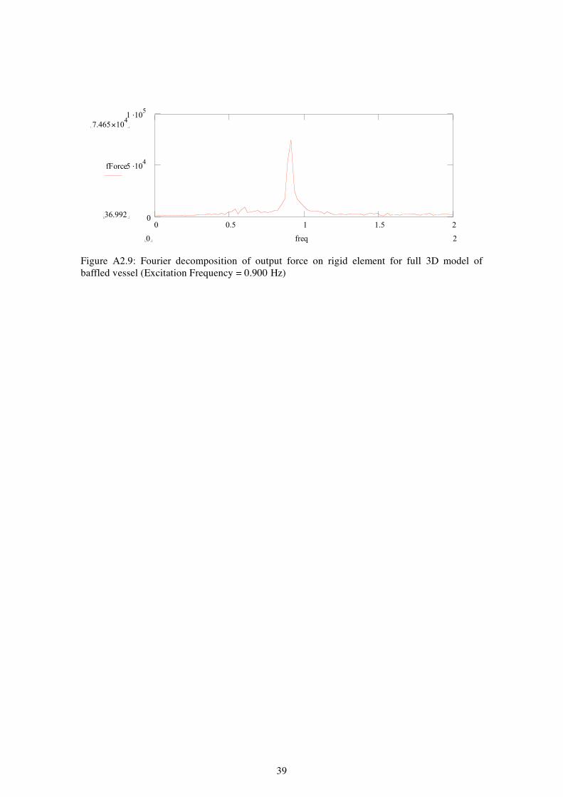
51 .10

47.465�10

4fForce5 .10

36.992 0 0 0.5 1 1.5 2

0 freq 2

Figure A2.9: Fourier decomposition of output force on rigid element for full 3D model of baffled vessel (Excitation Frequency = 0.900 Hz)

39

40

APPENDIX 3

Fourier results for Baffled Vessel – Fluid Fill Ratio 0.20

5 1.5 .10

5 1.061�10

5 1 .10

fForce

45 .10

35.9 0 0 0.5 1 1.5 2

0 freq 2

Figure A3.1: Fourier decomposition of output force on rigid element for full 3D model of baffled vessel (Excitation Frequency = 0.125 Hz)

5 2 .10

5 1.653�10

5 fForce1 .10

12.994 0 0 0.5 1 1.5 2

0 freq 2

Figure A3.2: Fourier decomposition of output force on rigid element for full 3D model of baffled vessel (Excitation Frequency = 0.275 Hz)

41

5 4 .10

5 3.289 10 �

5 fForce2 .10

18.72 0 0 0.5 1 1.5 2

0 freq 2

Figure A3.3: Fourier decomposition of output force on rigid element for full 3D model of baffled vessel (Excitation Frequency = 0.400 Hz)

5 4 .10

5 3.169 10 �

5 fForce2 .10

21.81 0 0 0.5 1 1.5 2

0 freq 2

Figure A3.4: Fourier decomposition of output force on rigid element for full 3D model of baffled vessel (Excitation Frequency = 0.500 Hz)

42

5 6 .10

5 5.827 10 �

5 4 .10

fForce

52 .10

38.546 0 0 0.5 1 1.5 2

0 freq 2

Figure A3.5: Fourier decomposition of output force on rigid element for full 3D model of baffled vessel (Excitation Frequency = 0.600 Hz)

5 6 .10

5 4.271 10 �

5 4 .10

fForce

52 .10

30.657 0 0 0.5 1 1.5 2

0 freq 2

Figure A3.6: Fourier decomposition of output force on rigid element for full 3D model of baffled vessel (Excitation Frequency = 0.650 Hz)

43

5 3 .10

5 2.216 10 �

5 2 .10

fForce

51 .10

24.708 0 0 0.5 1 1.5 2

0 freq 2

Figure A3.7: Fourier decomposition of output force on rigid element for full 3D model of baffled vessel (Excitation Frequency = 0.700 Hz)

5 1.5 .10

5 1.199 10 �

5 1 .10

fForce

45 .10

21.514 0 0 0.5 1 1.5 2

0 freq 2

Figure A3.8: Fourier decomposition of output force on rigid element for full 3D model of baffled vessel (Excitation Frequency = 0.800 Hz)

44

5 1.5 .10

5 1.2 10�

5 1 .10

fForce

45 .10

40.319 0 0 0.5 1 1.5 2

0 freq 2

Figure A3.9: Fourier decomposition of output force on rigid element for full 3D model of baffled vessel (Excitation Frequency = 0.900 Hz)

45

46

APPENDIX 4

Fourier results for Baffled Vessel – Fluid Fill Ratio 0.25

5 2 .10

5 1.554 10 �

5 fForce1 .10

74.117 0 0 0.5 1 1.5 2

0 freq 2

Figure A4.1: Fourier decomposition of output force on rigid element for full 3D model of baffled vessel (Excitation Frequency = 0.125 Hz)

5 3 .10

5 2.511 10 �

5 2 .10

fForce

51 .10

18.826 0 0 0.5 1 1.5 2

0 freq 2

Figure A4.2: Fourier decomposition of output force on rigid element for full 3D model of baffled vessel (Excitation Frequency = 0.275 Hz)

47

5 4 .10

5 3.93 10�

5 fForce2 .10

34.16 0 0 0.5 1 1.5 2

0 freq 2

Figure A4.3: Fourier decomposition of output force on rigid element for full 3D model of baffled vessel (Excitation Frequency = 0.400 Hz)

5 4 .10

5 3.516 10 �

5 fForce2 .10

43.111 0 0 0.5 1 1.5 2

0 freq 2

Figure A4.4: Fourier decomposition of output force on rigid element for full 3D model of baffled vessel (Excitation Frequency = 0.500 Hz)

48

6 1 .10

5 7.925 10 �

5 fForce5 .10

23.166 0 0 0.5 1 1.5 2

0 freq 2

Figure A4.5: Fourier decomposition of output force on rigid element for full 3D model of baffled vessel (Excitation Frequency = 0.600 Hz)

6 1 .10

5 6.111 10 �

5 fForce5 .10

10.871 0 0 0.5 1 1.5 2

0 freq 2

Figure A4.6: Fourier decomposition of output force on rigid element for full 3D model of baffled vessel (Excitation Frequency = 0.650 Hz)

49

5 4 .10

5 3.074 10 �

5 fForce2 .10

40.547 0 0 0.5 1 1.5 2

0 freq 2

Figure A4.7: Fourier decomposition of output force on rigid element for full 3D model of baffled vessel (Excitation Frequency = 0.700 Hz)

5 3 .10

5 2.078 10 �

5 2 .10

fForce

51 .10

64.325 0 0 0.5 1 1.5 2

0 freq 2

Figure A4.8: Fourier decomposition of output force on rigid element for full 3D model of baffled vessel (Excitation Frequency = 0.800 Hz)

50

53 .10

52.437 10�

52 .10

fForce

51 .10

39.79 0 0 0.5 1 1.5 2

0 freq 2

Figure A4.9: Fourier decomposition of output force on rigid element for full 3D model of baffled vessel (Excitation Frequency = 0.900 Hz)

51

Health and Safety Executive

Fluid structure interaction effects on and dynamic response of pressure vessels and tanks subjected to dynamic loading Part 3: Dynamic analysis of pressure vessel under earthquake, ship impact and blast loading

The Steel Construction Institute Silwood Park Ascot Berks SL5 7QN

As part of a suite of work looking at fluid interaction effects on (and the dynamic response of ) pressure vessels and tanks subjected to dynamic loading, this report details the findings of a series of explicit dynamic analyses on a computer modelled horizontal, cylindrical pressure vessel with semi-ellipsoidal heads, mounted on saddle supports. Using MSC Dytran software, the vessel was subjected to time history earthquake, blast and ship impact loadings. The results show that in the longitudinal direction, the tank-fluid system behaves essentially as a rigid body with small sloshing amplitude. Significant cross-sectional distortion is seen in the lateral direction with the maximum effects occurring in the centre of the tank. High stresses (90% of yield) occur in the extreme fibres of the tank shell structure at the supports. These, together with stresses from the operating internal pressure could lead to yielding.

This report and the work it describes were funded by the Health and Safety Executive (HSE). Its contents, including any opinions and/or conclusions expressed, are those of the authors alone and do not necessarily reflect HSE policy.

HSE Books

© Crown copyright 2007

First published 2007

All rights reserved. No part of this publication may bereproduced, stored in a retrieval system, or transmitted inany form or by any means (electronic, mechanical,photocopying, recording or otherwise) without the priorwritten permission of the copyright owner.

Applications for reproduction should be made in writing to:Licensing Division, Her Majesty’s Stationery Office,St Clements House, 2-16 Colegate, Norwich NR3 1BQor by e-mail to hmsolicensing@cabinet-office.x.gsi.gov.uk

ii

ACKNOWLEDGEMENTS

The authors would like to express their thanks to Mr Edwin Devries for his advice and technical support in using the software MSC Dytran. Our thanks also go to Mr Nigel Atkinson of MSC Software in providing a discounted cost for the software.

iii

iv

CONTENTS

EXECUTIVE SUMMARY VII

1 INTRODUCTION 11.1 VESSEL CONFIGURATION ON OFFSHORE PLATFORMS 11.2 MODELLING OF FLUID-STRUCTURE INTERACTION PROBLEM 61.3 ARBITRARY LAGRANGIAN EULERIAN FORMULATION 61.4 NUMERICAL CONSIDERATIONS 6

1.4.1 TIME STEP SIZE 6

1.4.2 ENERGY BALANCE 7

1.4.3 MASS SCALING AND SUBCYCLING 71.5 MODELLING OF TANK, SADDLE SUPPORTS AND FLUID 7

1.5.1 MESHING DETAILS AND ASSUMPTIONS 81.6 LATERAL EXCITATIONS 10

2 FLUID-STRUCTURE INTERACTION ANALYSIS AND RESULTS 162.1 INTRODUCTION 162.2 DESCRIPTION OF STRESSES IN TANK STRUCTURE 17

2.2.1 TIME HISTORY VARIATION OF STRESSES 17

2.2.2 LONGITUDINAL VARIATION OF EFFECTIVE STRESS IN TANK 35

2.2.3 CIRCUMFERENTIAL VARIATION OF EFFECTIVE STRESSES IN TANK 46

2.2.4 VARIATION OF SHELL LAYER STRESSES 46

2.2.5 COMPARISON WITH EARTHQUAKE AND BLAST EXCITATIONRESPONSES 53

2.2.6 BAFFLED VESSEL RESPONSE 532.3 DESCRIPTION OF FLUID PRESSURES 61

2.3.1 TIME HISTORY VARIATION OF FLUID PRESSURES 61

2.3.2 LONGITUDINAL VARIATION OF FLUID PRESSURE 62

2.3.3 CIRCUMFERENTIAL VARIATION OF FLUID PRESSURE 69

2.3.4 RADIAL VARIATION OF FLUID PRESSURE 69

2.3.5 VARIATION OF FLUID PRESSURE IN BAFFLED VESSEL 76

2.3.6 FLUID PRESSURE VARIATION IN VESSEL UNDER EARTHQUAKE AND

BLAST EXCITATIONS 762.4 COMPARISON BETWEEN ANALYTICAL RESULTS AND SIMPLIFIED

MODEL 882.5 CONCLUDING REMARKS 90

v

3 CONCLUSIONS 92 3.1 FURTHER WORK 93

4 REFERENCES 94

vi

EXECUTIVE SUMMARY

A series of explicit dynamic analyses were carried out on a horizontal, cylindrical pressure vessel with semi-ellipsoidal heads on saddle supports. The vessel was subjected to time history earthquake, blast and ship impact loadings.

The analyses were performed using the software MSC Dytran which is well suited to deal with fluid-structure problems. The Arbitrary Lagrangian Eulerian (ALE) method was used whereby the structure is modelled using Lagrangian elements while Eulerian elements are used for the fluid model. The structural and Eulerian regions are subsequently coupled by ALE surfaces where the structure serves as a boundary condition for the Eulerian region at the interfaces.

The results have shown that in the longitudinal direction (i.e. along the length of the tank), the tank-fluid system behaves essentially as a rigid body with small sloshing amplitude. In the lateral direction, the tank exhibits significant cross-sectional distortion with the maximum occurring at the centre of the tank. This arises mainly due to the significant flexibility of the tank away from the stiff ends.

It was also noted that high stresses (90% of yield) occur in the extreme fibres of the tank shell structure at the supports. Superposition of these stresses with the stresses from the operating internal pressure may lead to yielding.

A baffled vessel was also analysed and the results showed that the presence of the baffles significantly reduces the stresses in the tank structure.

A comparison of the numerical results with code predictions was carried out. The latter was based on the approximate procedure for rectangular tanks. As expected, the comparison showed significant differences. It is recommended that further studies be carried out to derive design guidance for horizontal cylindrical tanks with semi-0ellipsoidal heads.

vii

viii

1 INTRODUCTION

1.1 VESSEL CONFIGURATION ON OFFSHORE PLATFORMS

Tanks and pressure vessels are prominent on offshore production platforms where they perform various functions, which include diesel storage, separators, scrubbers, surge vessels and drums, coalescers, filters and heat exchangers. A typical layout is shown in Figure 1.The geometry and configuration of these tanks and pressure vessels differ according to the functional requirements. Rectangular tanks on elevated braced supports (Figure 2) are predominantly used for diesel storage while pressure vessels constitute a large proportion of production vessels where the configuration are either vertical or horizontal cylinders each with dished ends. Typical examples of the latter configurations are shown in Figures 3-4.

The vertical pressure vessels are usually welded to a continuous skirt, which is bolted to the deck structure (Figure 3). These vessels have high aspect ratios (H/R between 10 to 12) and small diameters (typically 600mm). The convective or sloshing pressures due to the fluid will not be significant for such vessels and the fluid mass can be assumed to move in unison with the tank under lateral excitation. The design complexity for such vessels lies in the number of attachment points, which results in differential accelerations being experienced by the vessel at the various support levels.

Horizontal cylindrical pressure vessels are fixed to two saddle supports (Figure 4), which are bolted to the deck structure. These vessels are the most common production vessels and the internal layout varies according to the functional requirements. Typically, such vessels will have internal baffles and various internal components such as vane packs, vortex breakers and splash plates, which will affect the fluid flow dynamics. The lateral excitation will result in both longitudinal (along length of tank) and lateral sloshing modes being excited with the sloshing magnitude governed by the dimensions of the tank, the fluid level and the magnitude and frequency content of the excitation.

Due to the prevalence of horizontal cylindrical pressure vessels with semi-ellipsoidal heads and the dearth of simplified design methods for such vessels under lateral excitation, the subsequent dynamic finite element analyses are geared towards understanding the behaviour of such vessels under various dynamic loadings and assessing the contribution of hydrodynamic pressure components to the effective wall and saddle support stresses.

1

Figure 1 Typical Layout of Equipment on Offshore Module

2

Figure 2 Typical Rectangular Tank for Diesel Storage on Offshore Module

3

Figure 3 Typical Vertical Cylindrical Tank on Offshore Module

4

Figure 4 Typical Horizontal Cylindrical Tank on Offshore Module

5

1.2 MODELLING OF FLUID-STRUCTURE INTERACTION PROBLEM

The dynamic finite element analyses for the horizontal cylindrical vessels with semi-ellipsoidal heads were carried out using the MSC Dytran software, which is based on explicit time domain methods. The software, developed by MSC Software Ltd, is well suited to dealing with fluid-structure interaction problems via a general coupling algorithm or an arbitrary Lagrangian Eulerian formulation. The general coupling algorithm is usually used for complex shapes undergoing arbitrary motions. For the vessel under consideration, the arbitrary Lagrangian Eulerian (ALE) formulation provides a faster solution without compromising the accuracy of the solution.

1.3 ARBITRARY LAGRANGIAN EULERIAN FORMULATION

Lagrangian meshes are particularly suited for the modelling of the structural elements as the elements deform with the material. Since the boundary nodes remain on the boundary throughout the evolution of the problem, the imposition of boundary conditions in Lagrangian meshes is straightforward. However, when the material undergoes severe deformation, the Lagrangian elements become similarly distorted and the accuracy of the elements deteriorates rapidly.

In the Eulerian method, the mesh is fixed in space while material flows through it. Eulerian meshes are, therefore, unchanged by the deformation of the material so that there is no degradation in accuracy of the elements due to material deformation. However, in Eulerian meshes, boundary nodes do not remain coincident with the boundary which requires the imposition of boundary conditions at points which are not nodes leading to severe complications.

The Arbitrary Lagrangian Eulerian formulation is a hybrid technique that combines the advantages of both the Eulerian and Lagrangian meshes. ALE descriptions are arbitrary combinations of the Eulerian and Lagrangian descriptions where arbitrary refers to the fact that the combination is specified by the user through selection of a mesh motion. The structure is modelled using Lagrangian elements while Eulerian elements are used for the fluid model. The structure and Eulerian regions are subsequently coupled by ALE surfaces where the structure serves as a boundary condition for the Eulerian region at the interfaces. The Eulerian material exerts a pressure on the structure at the interface causing deformation of the structure which results in a modification of the fluid flow field and hence in fluid-structure interaction.

1.4 NUMERICAL CONSIDERATIONS

In explicit time domain finite element analysis, several factors govern the accuracy, stability and cost of the solution. A good description of these factors is provided in the MSC Dytran Reference Manual [1] and by Belytschko et. al. [2]. A brief overview of these salient parameters is presented below.

1.4.1 Time Step Size

The time step size is usually set by the requirements to maintain stability of the integration scheme (usually central difference scheme). Explicit time integration is robust (i.e. procedure seldom aborts due to failure of numerical algorithm) but conditionally stable which implies that if the time step size exceeds a critical value � tcrit, the solution grows unboundedly. The critical time step is given by the Courant condition, which states that the critical time step must be smaller than the smallest natural period in the mesh for stability. This implies that the critical time step decreases with mesh refinement and increasing stiffness of the material. The cost of an

6

explicit analysis is therefore dependent only on the size of the model and the number of time steps.

1.4.2 Energy Balance

For non-linear problems, it is possible for instabilities to develop even when the Courant condition is observed. Such instabilities are not readily discernible by examining the results and can lead to large overprediction of displacements. Such instabilities are known as arrested instabilities and can be detected by an energy balance check due to the fact that they generate spurious energies, which lead to violation of the law of conservation of energy. Hence, in non-linear problems, energy balance can be used to check whether stability is maintained during the computational cycles.

1.4.3 Mass Scaling and Subcycling

The Courant condition imposes severe restrictions on the size of the time step to be used in an explicit analysis. The problem is particularly acute when the FE model contains only a few very small or stiff elements as the time step is set by these elements. Methods to circumvent this problem include:

• Mass Scaling: Masses of the stiffer elements are increased so that the time step size is not unduly reduced by these elements. Mass scaling is however not recommended in problems where high frequency effects are important.

• Subcycling: A smaller time step is used for the very small or stiff elements. In this case, the model is divided into subdomains with each subdomain integrated with its own stable time step.

1.5 MODELLING OF TANK, SADDLE SUPPORTS AND FLUID

The configuration and geometry of the tank selected for the dynamic finite element analyses is shown in Figure 5. The tank is fixed on saddle supports, which are bolted to the deck structure. Typically, the tank has several internal components and nozzle attachments, which affect the fluid flow and the distribution of stresses in the tank wall respectively.

4.5m

9.2 m

2:1 Ellipsoidal Head

Baffles 3.7 m

1.125 m

1.2 m 11.6 m 1.2 m

Figure 5 Horizontal Cylindrical Pressure Vessel with Semi-Ellipsoidal Heads (Liquid

Level = 3m)

7

However, given the variability in the layout of the internal components and nozzle attachments and the added modelling complexity, the subsequent finite element analyses were carried out for a tank without any internal components (apart from the baffles) and nozzle attachments. The effect of these components/nozzle attachments on the flow characteristics and the distribution of stresses in the tank structure need to be assessed in a separate study.

The dimensions for the selected tank were obtained from an actual knockout free water vessel. The thickness of the tank structure and support plates were:

Tank Shell Thickness: 33mm

Support Bottom Plate: 30mm

Support Stiffener Plate: 20mm

Support Web Plate: 25mm

Support Top Plate: 33mm

Baffle Thickness: 6mm

The operating pressure of the vessel is 8.0 bars with a design pressure of 27 bars. A summary of the element types and material types and properties is given in Table 1.

Element Type Material Density (kg/m3) Yield Stress (N/mm2)

Tank 4 noded Shell Steel 7850 385

Saddle 4 noded Shell Steel 7850 385

Fluid 8 noded Solid Water 1000 -

Table 1 Element Types and Material Properties

The 4 noded shell element is based on the Key-Hoff formulation, which is an improved version of the Belytschko-Tsay formulation as it can deal with warped element geometries. The shell element uses a 3-point Gauss integration and a transverse shear correction factor of 0.83333. The material properties for the shell element are assumed to be isotropic, elastoplastic with a Von Mises failure criterion. The 8 noded solid element uses one point Gauss integration and the material in the element has a stress tensor that consists only of the hydrodynamic pressure thereby being cheap to use.

1.5.1 Meshing Details and Assumptions

The mesh for the tank shell, saddle supports and the Eulerian region is shown in Figures 6 and 7 respectively. The mesh is refined at the support locations to accommodate the width of the support plates. To enable ALE coupling, the Eulerian mesh has the same degree of refinement as the Lagrangian mesh for the tank shell structure. This results in coinciding nodes at the interface between the Eulerian and Lagrangian meshes which are subsequently coupled via an ALE formulation. The Eulerian region is divided into 2 sub-regions, which comprise of a fluid region and a void region. As no material model is used to describe the void, the minimum pressure for the fluid is set to –1.0 bar. The equation of state for the fluid is polynomial in nature

8

where the pressure is related to the relative volume and specific internal energy via a cubic

equation.

Figure 6 Meshing Details for Tank and Saddle Supports (4-noded shell elements)

9

Figure 7 Meshing Details for Eulerian Region (8-noded solid elements) 1.6 LATERAL EXCITATIONS

The velocity time histories for the earthquake, ship impact and blast excitations were obtained from the Eatec study [3]. The time histories and corresponding acceleration response spectra are shown in Figures 8-13. The blast loading time history is of very short duration compared to the earthquake and ship impact loading and has the slightly higher peak velocity. Comparison of the secondary response spectra shows that:

• the blast loading (Y-direction), as defined in Figure 11, has higher acceleration values (peak value of 1.35g at 8 Hz) at all frequencies. There is also no well-defined tail region with peaks occurring at frequencies of 19 Hz (1.3g) and 40 Hz (0.85g)

• most of the energy in the earthquake loading is concentrated at low frequencies (0.05 – 4.0 Hz). The acceleration tails off to the zero period ground acceleration (ZPA) at higher frequencies and is relatively low (0.15g – X direction, 0.055g – Y direction) compared to the blast loading accelerations at similar frequencies

• the X direction ship impact response spectrum is similar to the earthquake spectra with high energy content at low frequencies and tailing off to an acceleration of approximately 0.095g at higher frequencies. In the Y direction, there is quite high energy content at the higher frequencies (similar to the blast loading) characterised by secondary peaks. The acceleration values (0.25 – 0.3g) at these peaks are, however, substantially lower than the corresponding blast loading accelerations at similar frequencies.

10

Vel

oci

ty (

m/s

)

0.40

0.30

0.20

0.10

0.00

-0.10

-0.20

-0.30

X-Direction

Y-Direction

0.00 0.25 0.50 0.75 1.00 1.25 1.50

Time (sec)

c i t srFigure 8 Ve lo y Time Hi to Fo Bla st Exci a ti oy r t n

11

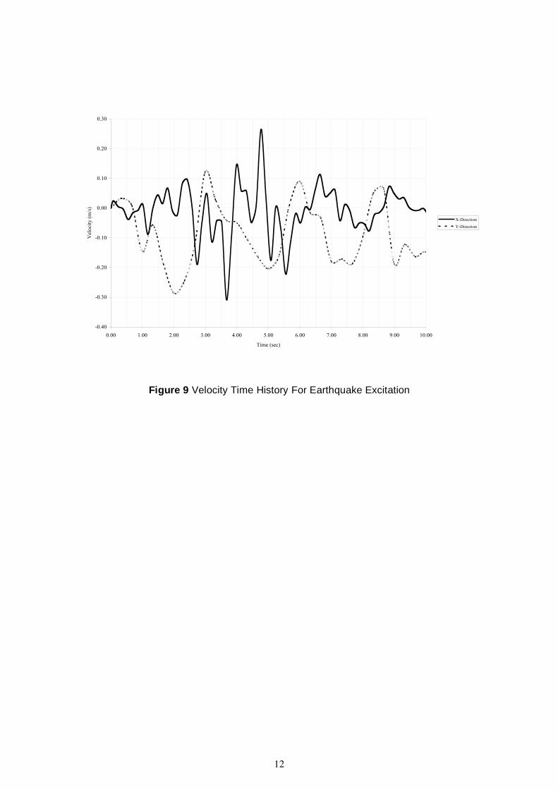
12

Figure 9 Velocity Time History For Earthquake Excitation

-0.40

-0.30

-0.20

-0.10

0.00

0.10

0.20

0.30

0.00 1.00 2.00 3.00 4.00 5.00 6.00 7.00 8.00 9.00 10.00

Time (sec)

Vel

oci

ty(m

/s)

X-Direction

Y-Direction

13

Figure 10 Velocity Time History For Ship Impact Loading

Figure 11 Secondary Response Spectra For Blast Excitation

-0.40

-0.30

-0.20

-0.10

0.00

0.10

0.20

0.30

0.40

0.00 1.00 2.00 3.00 4.00 5.00 6.00 7.00 8.00 9.00 10.00

Time (sec)

Vel

oci

ty(m

/s)

X-Direction

Y-Direction

0.00

0.20

0.40

0.60

0.80

1.00

1.20

1.40

1.60

0.0 5.0 10.0 15.0 20.0 25.0 30.0 35.0 40.0

Frequency (Hz)

Acc

eler

atio

n(g

)

Blast X-Dir

Blast Y-Dir

14

Figure 12 Secondary Response Spectra For Earthquake Excitation

Figure 13 Secondary Response Spectra For Ship Impact Excitation

0.00

0.05

0.10

0.15

0.20

0.25

0.30

0.35

0.40

0.45

0.0 5.0 10.0 15.0 20.0 25.0 30.0 35.0 40.0

Freauency (Hz)

Acc

eler

atio

n(g

)

Earthquake X-Dir

Earthquake Y-Dir

0.00

0.10

0.20

0.30

0.40

0.50

0.60

0.70

0.0 5.0 10.0 15.0 20.0 25.0 30.0 35.0 40.0

Frequency (Hz)

Acc

eler

atio

n(g

)

Ship Impact - X-Dir

Ship Impact Y-Dir

2 Fluid-Structure Interaction Analysis and Results

2.1 INTRODUCTION

A series of dynamic finite element analyses have been carried out to assess the structural response of the tank and the fluid response under different lateral excitations. The analyses and results pertain mainly to the un-baffled vessel. However, the effect of baffles on the stresses in the vessel wall and on the fluid pressures was also examined. Unless otherwise specified, the subsequent description of the analyses and results pertain to the un-baffled vessel. The analyses included

• Blast Excitation – X (longitudinal) and Y (lateral) directions simultaneously

• Earthquake Excitation – X and Y directions simultaneously

• Ship Impact Excitation – X direction only

• Ship Impact Excitation – Y direction only

• Ship Impact – X and Y directions simultaneously

The time history, longitudinal and circumferential variation of stresses in the tank shell and the fluid pressures were obtained at various locations. The variation of stresses and fluid pressures along the length of the tank (i.e. between the right-cylinder-ellipsoid junction and left-cylinder-ellipsoid junction) is shown at the following heights:

• Bottom of tank

• Horn of Saddle i.e. level at junction between outer saddle plate stiffener and tank structure

• Free Surface – level of quiescent fluid (3m above bottom of tank)

• Top of tank

The circumferential variation of stresses/fluid pressures are shown at the following locations:

• Right-cylinder-ellipsoid-junction

• Right support location

• Right baffle location – for comparison between baffled/un-baffled vessels

• Centre of tank

The time history variation of the stresses and fluid pressures is also shown at the same locations albeit for 3 elements only (corresponding to heights at bottom of tank, horn of saddle and free surface) at each location. Only results to the right of the centre of the tank are shown as the distribution of stresses/fluid pressures can be assumed to be symmetrical (section 2.2.2 and section 2.3.2).

Further insight into the effect of the hydrodynamic components is provided by comparison against static results for the fluid-filled vessel and against results from dynamic analyses of the empty tank under the same lateral excitations.

The state of stress is described in terms of an effective (Von Mises) stress at the mid-layer of the shell. The stresses in the inner and outer layers of the shell can be higher (although the trend in behaviour is the same) than the mid-layer stress depending on the direction of the stress component due to bending. However, for purposes of comparison and assessment of the

15

behaviour of the tank structure, only the mid-layer stress values are quoted unless otherwise indicated.

For the ship impact excitation (X and Y directions simultaneously), the effective stress is broken down into its components (i.e. longitudinal stress, circumferential stress and tangential shear stress) to provide a thorough description of the distribution of stresses in the tank structure and saddle supports.

2.2 DESCRIPTION OF STRESSES IN TANK STRUCTURE

The first part of the results examines the distribution of stresses in the vessel structure under the different lateral excitations. The main focus of the results in on the ship impact excitation, as the input accelerations in this case are significantly higher than the corresponding earthquake excitations. Although the magnitude of the accelerations for the blast excitation is higher than that for the ship impact excitation, the duration is much shorter (1.5 sec). However, a comparison of the time history response for the various excitations is provided and the differences in response are highlighted.

The resultant stresses in the vessel wall are also highlighted by comparison against static and empty tank results. Finally, the fluid pressure contribution is addressed to provide further insight into the contribution of the various hydrodynamic components to the overall response of the vessel.

2.2.1 Time History Variation of Stresses

The variation of effective stresses at different levels and locations under different ship impact excitation scenarios is shown in Figures 14-17 for the X-direction excitation, Figures 18-21 for the Y-direction excitation and Figures 22-25 for the combined X and Y direction excitations. Comparison of the results leads to the following observations:

• The main contribution to the effective stresses results from the Y-direction excitation. The peak stress in the tank structure due to the X-direction excitation only occurs at approximately 0.1 sec and is significantly lower than the maximum peak stress due to the Y-direction excitation only.

• Highest peak stresses occur at the level of the horn of the saddle at the support locations. The peak stresses at the various heights decay rapidly after 1.3 sec tailing off to nearly constant values beyond 5.0 sec. The latter values correspond approximately to the stress level under static conditions (Figures 26-27) where it is noted that the maximum stress occurs in the region of the horn of the saddle.

• The stress at the free surface level increases towards the centre of the tank in the case of the Y-direction and XY-direction excitations. This results primarily from the increased flexibility of the tank away from the stiff ends and supports, which leads to increased lateral deformations.

• For the Y direction excitation only and the combined X and Y direction excitation, the variation of effective stresses is of the damped periodic type with a predominant period of approximately 0.5 sec. The stress amplitude at time t = 1.3 sec is approximately halved in about 2 to 3 cycles which suggests a damping ratio between 4 to 5% of critical in the tank-fluid modes of vibration.

The low stresses in the tank structure due to the X-direction excitation only was further investigated by applying the Y excitation values in the X-direction. The results are shown in Figures 28-31 and it is observed that the magnitude on the peak stresses has undergone no

16

significant change. The difference in the level of stresses in the two excitation directions lies in the fact that the X-direction motion results in a rigid-body displacement of the structure as shown in Figures 32-33. The X displacements along the length of the tank and in the circumferential direction are approximately the same for all nodal points at the various time instants shown.

17

18

Figure 14 Variation of Effective Stress with Time at Right-Cylinder-Ellipsoid-Junction

(Ship Impact – X Direction)

Figure 15 Variation of Effective Stress with Time at Right Support Location (Ship Impact

– X Direction)

0.0

2.0

4.0

6.0

8.0

10.0

12.0

14.0

0.0 0.5 1.0 1.5 2.0 2.5 3.0 3.5 4.0 4.5 5.0

Time (sec)

Eff

ecti

ve

Str

ess

(N/m

m^2)

Bottom of Tank

Horn of Saddle

Free Surface

0.0

5.0

10.0

15.0

20.0

25.0

30.0

0.0 0.5 1.0 1.5 2.0 2.5 3.0 3.5 4.0 4.5 5.0

Time (sec)

Eff

ecti

ve

Str

ess

(N/m

m^2)

Bottom of Tank

Horn of Saddle

Free Surface

19

Figure 16 Variation of Effective Stress with Time at Right Baffle Location (Ship Impact –X Direction)

Figure 17 Variation of Effective Stress with Time at Centre of Tank (Ship Impact – X

Direction)

0.0

2.0

4.0

6.0

8.0

10.0

12.0

14.0

16.0

0.0 0.5 1.0 1.5 2.0 2.5 3.0 3.5 4.0 4.5 5.0

Time (sec)

Eff

ecti

ve

Str

ess

(N/m

m^2)

Bottom of Tank

Horn of Saddle

Free Surface

0.0

1.0

2.0

3.0

4.0

5.0

6.0

7.0

0.0 0.5 1.0 1.5 2.0 2.5 3.0 3.5 4.0 4.5 5.0

Time (sec)

Eff

ecti

ve

Str

ess

(N/m

m^2)

Bottom of Tank

Horn of Saddle

Free Surface

20

Figure 18 Variation of Effective Stress with Time at Right-Cylinder-Ellipsoid-Junction

(Ship Impact – Y Direction)

Figure 19 Variation of Effective Stress with Time at Right Support Location (Ship Impact

– Y Direction)

0.0

10.0

20.0

30.0

40.0

50.0

60.0

70.0

80.0

90.0

100.0

0.0 0.5 1.0 1.5 2.0 2.5 3.0 3.5 4.0 4.5 5.0

Time (sec)

Eff

ecti

ve

Str

ess

(N/m

m^2)

Bottom of Tank

Horn of Saddle

Free Surface

0.0

20.0

40.0

60.0

80.0

100.0

120.0

140.0

160.0

0.0 0.5 1.0 1.5 2.0 2.5 3.0 3.5 4.0 4.5 5.0

Time (sec)

Eff

ecti

ve

Str

ess

(N/m

m^2)

Bottom of Tank

Horn of Saddle

Free Surface

21

Figure 20 Variation of Effective Stress with Time at Right Baffle Location (Ship Impact –

Y Direction)

Figure 21 Variation of Effective Stresses with Time at Centre of Tank (Ship Impact – YDirection)

0.0

5.0

10.0

15.0

20.0

25.0

30.0

35.0

40.0

0.0 0.5 1.0 1.5 2.0 2.5 3.0 3.5 4.0 4.5 5.0

Time (sec)

Eff

ecti

ve

Str

ess

(N/m

m^2)

Bottom of Tank

Horn of Saddle

Free Surface

0.0

5.0

10.0

15.0

20.0

25.0

30.0

35.0

40.0

0.0 0.5 1.0 1.5 2.0 2.5 3.0 3.5 4.0 4.5 5.0

Time (sec)

Eff

ecti

ve

Str

ess

(N/m

m^2)

Bottom of Tank

Horn of Saddle

Free Surface

22

Figure 22 Variation of Effective Stress with Time at Right-Cylinder-Ellipsoid-Junction

(Ship Impact – XY Direction)

Figure 23 Variation of Effective Stress with Time at Right Support Location (Ship Impact

– XY Direction)

0.0

10.0

20.0

30.0

40.0

50.0

60.0

70.0

80.0

90.0

100.0

0.0 1.0 2.0 3.0 4.0 5.0 6.0 7.0 8.0 9.0 10.0

Time (sec)

Eff

ecti

ve

Str

ess

(N/m

m^2)

Bottom of Tank

Horn of Saddle

Free Surface

0.0

20.0

40.0

60.0

80.0

100.0

120.0

140.0

160.0

0.0 1.0 2.0 3.0 4.0 5.0 6.0 7.0 8.0 9.0 10.0

Time (sec)

Eff

ecti

ve

Str

ess

(N/m

m^2)

Bottom of Tank

Horn of Saddle

Free Surface

23

Figure 24 Variation of Effective Stress with Time at Right Baffle Location (Ship Impact

– XY Direction)

Figure 25 Variation of Effective Stress with Time at Centre of Tank (Ship Impact – XY

Direction)

0.0

5.0

10.0

15.0

20.0

25.0

30.0

35.0

40.0

0.0 1.0 2.0 3.0 4.0 5.0 6.0 7.0 8.0 9.0 10.0

Time (sec)

Eff

ecti

ve

Str

ess

(N/m

m^2)

Bottom of Tank

Horn of Saddle

Free Surface

0.0

5.0

10.0

15.0

20.0

25.0

30.0

35.0

40.0

0.0 1.0 2.0 3.0 4.0 5.0 6.0 7.0 8.0 9.0 10.0

Time (sec)

Eff

ecti

ve

Str

ess

(N/m

m^2)

Bottom of Tank

Horn of Saddle

Free Surface

24

Figure 26 Variation of Effective Stress at Various Heights along Length of Tank (Static)

Figure 27 Circumferential Variation of Effective Stress at Various Locations (Static)

0.0

2.0

4.0

6.0

8.0

10.0

12.0

14.0

16.0

-7.0 -6.0 -5.0 -4.0 -3.0 -2.0 -1.0 0.0 1.0 2.0 3.0 4.0 5.0 6.0 7.0

Distance Along Tank (m)

Eff

ecti

ve

Str

ess

(N/m

m^2)

Bottom of Tank

Horn of Saddle

Free Surface

Top of Tank

0.0

2.0

4.0

6.0

8.0

10.0

12.0

14.0

16.0

-2.25 -1.75 -1.25 -0.75 -0.25 0.25 0.75 1.25 1.75 2.25

Circumferential Height (m)

Eff

ecti

ve

Str

ess

(N/m

m^2)

Right Cylinder to Ellipsoid Junction

Right Support location

Right Baffle Location

Centre of Tank

25

Figure 28 Variation of Effective Stress with Time at Right-Cylinder-Ellipsoid-Junction

(Ship Impact – X Direction – Y Excitation Values)

Figure 29 Variation of Effective Stress with Time at Right Support Location (Ship Impact– X Direction – Y Excitation values)

0.0

2.0

4.0

6.0

8.0

10.0

12.0

14.0

0.0 0.5 1.0 1.5 2.0 2.5 3.0 3.5 4.0 4.5 5.0

Time (sec)

Eff

ecti

ve

Str

ess

(N/m

m^2)

Bottom of Tank

Horn of Saddle

Free Surface

0.0

5.0

10.0

15.0

20.0

25.0

30.0

0.0 0.5 1.0 1.5 2.0 2.5 3.0 3.5 4.0 4.5 5.0

Time (sec)

Eff

ecti

ve

Str

ess

(N/m

m^2)

Bottom of Tank

Horn of Saddle

Free Surface

26

Figure 30 Variation of Effective Stress with Time at Right Baffle Location (Ship Impact –

X Direction – Y Excitation Values)

0.0

2.0

4.0

6.0

8.0

10.0

12.0

14.0

0.0 0.5 1.0 1.5 2.0 2.5 3.0 3.5 4.0 4.5 5.0

Time (sec)

Eff

ecti

ve

Str

ess

(N/m

m^2)

Bottom of Tank

Horn of Saddle

Free Surface

27

Figure 31 Variation of Effective Stress with Time at Centre of Tank (Ship Impact – X

Direction – Y Excitation Values)

Figure 32 Circumferential Variation of Longitudinal (X) Displacement at Right-Cylinder-

Ellipsoid-Junction (Ship Impact – X Direction – Y Excitation Values)

0.0

1.0

2.0

3.0

4.0

5.0

6.0

7.0

0.0 0.5 1.0 1.5 2.0 2.5 3.0 3.5 4.0 4.5 5.0

Time (sec)

Eff

ecti

ve

Str

ess

(N/m

m^2)

Bottom of Tank

Horn of Saddle

Free Surface

30.0

35.0

40.0

45.0

50.0

55.0

60.0

65.0

-2.25 -1.75 -1.25 -0.75 -0.25 0.25 0.75 1.25 1.75 2.25

Circumferential Height (m)

Dis

pla

cem

ent

(mm

)

t = 0.4 sec

t = 1.1 sec

t = 1.5 sec

t = 2.1 sec

t = 2.8 sec

65.0

60.0

55.0

50.0

45.0

40.0

35.0

30.0

Dis

pla

cem

ent

(mm

)

t = 0.4 sec

t = 1.1 sec

t = 1.5 sec

t = 2.1 sec

t = 2.8 sec

-7.00 -6.00 -5.00 -4.00 -3.00 -2.00 -1.00 0.00 1.00 2.00 3.00 4.00 5.00 6.00 7.00

Distance Along Tank (m)

Figure 33 Variation of Longitudinal (X) Displacement along Centre of Tank (Ship Impact

– X Direction – Y Excitation Values)

It is therefore possible to assume that the forces/moments, generated by the longitudinal (along the length of the tank) motion of the tank, consists of contributions from the rigid-impulsive and sloshing components.

Examination of the lateral (Y) displacement pattern (Figures 34-37) under the Y direction excitation shows that the maximum displacement occurs at the centre of the tank with a maximum relative displacement of approximately 14mm between the cylinder to ellipsoid junction and the centre of the tank. Circumferentially, the maximum displacement occurs just above the centre line of the tank with a maximum relative displacement of approximately 45mm between the latter nodal position and the bottom of the tank (Figure 37).

This is consistent with the increase in stress level in the region of the free surface towards the centre of the tank observed earlier. The fluid motion in the lateral direction causes a bulging out and ovalling of the tank and the circumferential distortion increases from the cylinder-ellipsoid-junction towards the centre of the tank. In this particular case, both sloshing and flexible-impulsive (i.e. coupled fluid-tank) modes of vibration are excited.

The effect of the flexible-impulsive and sloshing modes is better illustrated by comparison against results from an empty tank under the same lateral excitation. This is shown in Figures 38-41 and it is noted that

• The rapid decay in the peak effective stresses for the fluid-filled tank under the simultaneous application of the X and Y excitations contrasts with the steady decrease in peak stresses in the case of the empty tank under similar excitation. This suggests a high level of damping in the fluid-filled tank. As mentioned earlier, the damping level in the flexible-impulsive modes is found to be approximately 4 to 5% of critical. In the case of

28

the empty tank, there is no significant inherent energy dissipation mechanism, which explains the higher peak stresses beyond 4.0 sec.

• Although the stress level is significantly higher in the tank-fluid system, the variation in stress at the different locations with time, in the empty tank case, is similar with the maximum peak stress again occurring at the level of the horn of the saddle at the support locations. The peak stresses at the level of the free surface, at the centre of the tank, in the case of the empty tank are, however, approximately the same as those at the level of the horn of the saddle and at the bottom of the tank (cf. Figures 25 and 41). This is due to the fact that there is less cross-sectional distortion of the tank shell (no sloshing and coupled fluid-tank motion) in this case compared to the fluid-filled tank.

65.0

60.0

55.0

50.0

45.0

40.0

35.0

30.0

Dis

pla

cem

ent

(mm

)

t = 1.1 sec

t = 1.3 sec

t = 1.6 sec

t = 2.3 sec

t = 2.8 sec

-7.0 -6.0 -5.0 -4.0 -3.0 -2.0 -1.0 0.0 1.0 2.0 3.0 4.0 5.0 6.0 7.0

Distance Along Tank (m)

Figure 34 Variation of Lateral (Y) Displacement along Bottom of Tank (Ship Impact – Y

Direction)

29

30

Figure 35 Variation of Lateral (Y) Displacement along Centre of Tank (Ship Impact – Y

Direction)

Figure 36 Circumferential Variation of Lateral (Y) Displacement at Right-Cylinder-

Ellipsoid-Junction (Ship Impact – Y Direction)

45.0

50.0

55.0

60.0

65.0

70.0

75.0

80.0

85.0

90.0

-7.0 -6.0 -5.0 -4.0 -3.0 -2.0 -1.0 0.0 1.0 2.0 3.0 4.0 5.0 6.0 7.0

Distance Along Tank (m)

Dis

pla

cem

ent

(mm

)

t = 1.1 sec

t = 1.3 sec

t = 1.6 sec

t = 2.3 sec

t = 2.8 sec

35.0

40.0

45.0

50.0

55.0

60.0

65.0

70.0

75.0

80.0

-2.25 -1.75 -1.25 -0.75 -0.25 0.25 0.75 1.25 1.75 2.25

Circumferential Height (m)

Dis

pla

cem

ent

(mm

)

t = 1.1 sec

t = 1.3 sec

t = 1.6 sec

t = 2.3 sec

t = 2.8 sec

90.0

80.0

70.0

60.0

50.0

40.0

30.0

Dis

pla

cem

ent

(mm

)

t = 1.1 sec

t = 1.3 sec

t = 1.6 sec

t = 2.3 sec

t = 2.8 sec

-2.25 -1.75 -1.25 -0.75 -0.25 0.25 0.75 1.25 1.75 2.25

Circumferential Height (m)

Figure 37 Circumferential Variation of Lateral (Y) Displacement at Centre of Tank (Ship

Impact – Y Direction)

31

32

Figure 38 Variation of Effective Stress with Time at Right-Cylinder-Ellipsoid-Junction(Ship Impact – XY Direction – Empty Tank)

Figure 39 Variation of Effective Stress with Time at Right Support Location (Ship Impact

– XY Direction – Empty Tank)

0.0

5.0

10.0

15.0

20.0

25.0

30.0

0.0 1.0 2.0 3.0 4.0 5.0 6.0 7.0 8.0 9.0 10.0

Time (sec)

Eff

ecti

ve

Str

ess

(N/m

m^2)

Bottom of Tank

Horn of Saddle

Free Surface

0.0

5.0

10.0

15.0

20.0

25.0

30.0

35.0

40.0

45.0

0.0 1.0 2.0 3.0 4.0 5.0 6.0 7.0 8.0 9.0 10.0

Time (sec)

Eff

ecti

ve

Str

ess

(N/m

m^2)

Bottom of Tank

Horn of Saddle

Free Surface

33

Figure 40 Variation of Effective Stress with Time at Right Baffle Location (Ship Impact –XY Direction – Empty Tank)

Figure 41 Variation of Effective Stress with Time at Centre of Tank (Ship Impact – XYDirection – Empty Tank)

0.0

2.0

4.0

6.0

8.0

10.0

12.0

14.0

0.0 1.0 2.0 3.0 4.0 5.0 6.0 7.0 8.0 9.0 10.0

Time (sec)

Eff

ecti

ve

Str

ess

(N/m

m^2)

Bottom of Tank

Horn of Saddle

Free Surface

0.0

2.0

4.0

6.0

8.0

10.0

12.0

14.0

16.0

18.0

20.0

0.0 1.0 2.0 3.0 4.0 5.0 6.0 7.0 8.0 9.0 10.0

Time (sec)

Eff

ecti

ve

Str

ess

(N/m

m^2)

Bottom of Tank

Horn of Saddle

Free Surface

2.2.2 Longitudinal Variation of Effective Stress in Tank

The variation of stress along the length of the tank at various locations is shown in Figures 42-45 for the empty tank and in Figures 46-49 for the fluid-filled tank. Both sets of results pertain to the simultaneous application of the X and Y excitations with the results quoted at the respective peak effective stresses in the time histories. It is observed that the trend is similar in both cases and it is noted that

• The maximum stress occurs at the level of the horn of the saddle at the support locations as noted earlier. High stresses are also generated at the junction between the cylinder and ellipsoidal head at the level of the bottom of the tank.

• Stresses along the top of the tank for the fluid-filled vessel are higher than for the empty vessel due to the increased cross-sectional distortion and sloshing of the fluid.

• At the level of the free surface, the maximum stress for the fluid-filled tank exceeds that for the empty tank by a factor of approximately 2.8. This can be attributed to a combination of fluid sloshing and coupled fluid-tank motion.

Comparison against static stress distribution for both the empty tank and fluid-filled tank is shown in Figures 50-57 via a normalised effective stress. The latter is obtained by dividing the stress in the element (for the fluid-filled and empty vessels under simultaneous X and Y excitations) by the corresponding static stress value for a fluid-filled tank. The results show that the dynamic excitation induces large differences at the cylinder to ellipsoid junctions and at the support locations. The substantially higher normalised stresses at the centre of the tank along the free surface reflect the fact that the static stress value at the location is very low (0.1 N/mm2) compared to the dynamic stresses (approximately 16 N/mm2 for empty tank and approximately 40 N/mm2 for the fluid-filled tank). The latter arises primarily from the lateral deformation of the tank due to the combination of sloshing, rigid-impulsive and flexible-impulsive modes of vibration mentioned earlier.

The breakdown of the effective stress into its various components for the fluid-filled tank under lateral excitation is shown in Figures 58-61 at a time instant of 1.3 sec (where the peak stress occurs). It is observed that

• The maximum longitudinal stress component at the bottom of the tank is consistent with overall longitudinal bending with maximum longitudinal stresses occurring at the supports and at mid-span.

• The high tangential shear stresses at the cylinder to ellipsoid junctions are consistent with the fact the head stiffens the shell in the region of the saddle supports. This causes most of the tangential shear stresses to be carried across the saddle to the head and then the load is transferred back to the head side of the saddle.

• The high circumferential stresses at the support locations at the level of the horn of the saddle are due to the fact that the load must be transferred from the shell to the supports.

34

35

Figure 42 Variation of Effective Stress along Level of Bottom of Tank (Ship Impact –XY Direction – Empty Tank)

Figure 43 Variation of Effective Stress along Level of Horn of Saddle (Ship Impact –XY Direction – Empty Tank)

0.0

5.0

10.0

15.0

20.0

25.0

-7.0 -6.0 -5.0 -4.0 -3.0 -2.0 -1.0 0.0 1.0 2.0 3.0 4.0 5.0 6.0 7.0

Distance Along Tank (m)

Eff

ecti

ve

Str

ess

(N/m

m^2)

t = 1.15 sec

t = 1.90 sec

t = 2.85 sec

t = 4.65 sec

t = 5.50 sec

0.0

5.0

10.0

15.0

20.0

25.0

30.0

35.0

40.0

45.0

-7.0 -6.0 -5.0 -4.0 -3.0 -2.0 -1.0 0.0 1.0 2.0 3.0 4.0 5.0 6.0 7.0

Distance Along Tank (m)

Eff

ecti

ve

Str

ess

(N/m

m^2)

t = 1.15 sec

t = 1.90 sec

t = 2.85 sec

t = 4.65 sec

t = 5.50 sec

36

Figure 44 Variation of Effective Stress along Level of Free Surface of Tank (Ship Impact– XY Direction – Empty Tank)

Figure 45 Variation of Effective Stress along Level of Top of Tank (Ship Impact – XYDirection – Empty Tank)

0.0

2.0

4.0

6.0

8.0

10.0

12.0

14.0

16.0

18.0

-7.0 -6.0 -5.0 -4.0 -3.0 -2.0 -1.0 0.0 1.0 2.0 3.0 4.0 5.0 6.0 7.0

Distance Along Tank (m)

Eff

ecti

ve

Str

ess

(N/m

m^2)

t = 1.15 sec

t = 1.90 sec

t = 2.85 sec

t = 4.65 sec

t = 5.50 sec

0.0

1.0

2.0

3.0

4.0

5.0

6.0

7.0

-7.0 -6.0 -5.0 -4.0 -3.0 -2.0 -1.0 0.0 1.0 2.0 3.0 4.0 5.0 6.0 7.0

Distance Along tank (m)

Eff

ecti

ve

Str

ess

(N/m

m^2)

t = 1.15 sec

t = 1.90 sec

t = 2.85 sec

t = 4.65 sec

t = 5.50 sec

37

Figure 46 Variation of Effective Stress along Level of Bottom of Tank (Ship Impact – XYDirection)

Figure 47 Variation of Effective Stress along Level of Horn of Saddle (Ship Impact – XY

Direction)

0.0

10.0

20.0

30.0

40.0

50.0

60.0

70.0

80.0

-7.0 -6.0 -5.0 -4.0 -3.0 -2.0 -1.0 0.0 1.0 2.0 3.0 4.0 5.0 6.0 7.0

Distance Along Tank (m)

Eff

ecti

ve

Str

ess

(N/m

m^2)

t = 1.3 sec

t = 1.7 sec

t = 2.2 sec

t = 2.7 sec

t = 3.2 sec

t = 5.0 sec

0.0

20.0

40.0

60.0

80.0

100.0

120.0

140.0

-7.0 -6.0 -5.0 -4.0 -3.0 -2.0 -1.0 0.0 1.0 2.0 3.0 4.0 5.0 6.0 7.0

Distance Along Tank (m)

Eff

ecti

ve

Str

ess

(N/m

m^2)

t = 1.3 sec

t = 1.7 sec

t = 2.2 sec

t = 2.7 sec

t = 3.2 sec

t = 5.0 sec

38

Figure 48 Variation of Effective Stress along Level of Free Surface of Tank (Ship Impact– XY Direction)

Figure 49 Variation of Effective Stress along Level of Top of Tank (Ship Impact – XY

Direction)

0.0

5.0

10.0

15.0

20.0

25.0

30.0

35.0

40.0

45.0

50.0

-7.0 -6.0 -5.0 -4.0 -3.0 -2.0 -1.0 0.0 1.0 2.0 3.0 4.0 5.0 6.0 7.0

Distance Along Tank (m)

Eff

ecti

ve

Str

ess

(N/m

m^2)

t = 1.3 sec

t = 1.7 sec

t = 2.2 sec

t = 2.7 sec

t = 3.2 sec

t = 5.0 sec

0.0

2.0

4.0

6.0

8.0

10.0

12.0

-7.0 -6.0 -5.0 -4.0 -3.0 -2.0 -1.0 0.0 1.0 2.0 3.0 4.0 5.0 6.0 7.0

Distance Along Tank (m)

Eff

ecti

ve

Str

ess

(N/m

m^2)

t = 1.3 sec

t = 1.7 sec

t = 2.2 sec

t = 2.7 sec

t = 3.2 sec

t = 5.0 sec

39

Figure 50 Variation of Normalised Effective Stress along Level of Bottom of Tank (ShipImpact – XY Direction – Empty Tank)

Figure 51 Variation of Normalised Effective Stress along Level of Horn of Saddle (shipImpact – XY Direction – Empty Tank)

0.0

2.0

4.0

6.0

8.0

10.0

12.0

-7.0 -6.0 -5.0 -4.0 -3.0 -2.0 -1.0 0.0 1.0 2.0 3.0 4.0 5.0 6.0 7.0

Distance Along Tank (m)

Norm

alis

edE

ffec

tive

Str

ess

t = 1.15 sec

t = 1.90 sec

t = 2.85 sec

t = 4.65 sec

t = 5.50 sec

0.0

0.5

1.0

1.5

2.0

2.5

3.0

3.5

-7.0 -6.0 -5.0 -4.0 -3.0 -2.0 -1.0 0.0 1.0 2.0 3.0 4.0 5.0 6.0 7.0

Distance Along Tank (m)

Norm

alis

edE

ffec

tive

Str

ess

t = 1.15 sec

t = 1.90 sec

t = 2.85 sec

t = 4.65 sec

t = 5.5 sec

40

Figure 52 Variation of Normalised Effective Stress along Level of Free Surface of Tank(Ship Impact – XY Direction – Empty tank)

Figure 53 Variation of Normalised Effective Stress along Level of Top of Tank (ShipImpact – XY Direction – Empty Tank)

0.0

20.0

40.0

60.0

80.0

100.0

120.0

140.0

160.0

180.0

-7.0 -6.0 -5.0 -4.0 -3.0 -2.0 -1.0 0.0 1.0 2.0 3.0 4.0 5.0 6.0 7.0

Distance Along tank (m)

Norm

alis

edE

ffec

tive

Str

ess

t = 1.15 sec

t = 1.90 sec

t = 2.85 sec

t = 4.65 sec

t = 5.50 sec

0.0

2.0

4.0

6.0

8.0

10.0

12.0

-7.0 -6.0 -5.0 -4.0 -3.0 -2.0 -1.0 0.0 1.0 2.0 3.0 4.0 5.0 6.0 7.0

Distance Along Tank (m)

Norm

alis

edE

ffec

tive

Str

ess

t = 1.15 sec

t = 1.90 sec

t = 2.85 sec

t = 4.65 sec

t = 5.50 sec

41

Figure 54 Variation of Normalised Effective Stress along Level of Bottom of Tank (ShipImpact – XY Direction)

Figure 55 Variation of Normalised Effective Stress along Level of Horn of Saddle (Ship

Impact – XY Direction)

0.0

2.5

5.0

7.5

10.0

12.5

15.0

17.5

20.0

22.5

25.0

-7.0 -6.0 -5.0 -4.0 -3.0 -2.0 -1.0 0.0 1.0 2.0 3.0 4.0 5.0 6.0 7.0

Distance Along Tank (m)

Norm

alis

edE

ffec

tive

Str

ess

t = 1.3 sec

t = 1.7 sec

t = 2.2 sec

t = 2.7 sec

t = 3.2 sec

t = 5.0 sec

0.0

2.0

4.0

6.0

8.0

10.0

12.0

-7.0 -6.0 -5.0 -4.0 -3.0 -2.0 -1.0 0.0 1.0 2.0 3.0 4.0 5.0 6.0 7.0

Distance Along Tank (m)

Norm

alis

edE

ffec

tive

Str

ess

t = 1.3 sec

t = 1.7 sec

t = 2.2 sec

t = 2.7 sec

t = 3.2 sec

t = 5.0 sec

42

Figure 56 Variation of Normalised Effective Stress along Level of Free Surface of Tank(Ship Impact – XY Direction)

Figure 57 Variation of Normalised Effective Stress along Level of Top of Tank (ShipImpact – XY Direction)

0

50

100

150

200

250

300

350

400

-7 -6 -5 -4 -3 -2 -1 0 1 2 3 4 5 6 7

Distance Along Tank (m)

Norm

alis

edE

ffec

tive

Str

ess

t = 1.3 sec

t = 1.7 sec

t = 2.2 sec

t = 2.7 sec

t = 3.2 sec

t = 5.0 sec

0.0

2.0

4.0

6.0

8.0

10.0

12.0

14.0

16.0

-7.0 -6.0 -5.0 -4.0 -3.0 -2.0 -1.0 0.0 1.0 2.0 3.0 4.0 5.0 6.0 7.0

Distance Along Tank (m)

Norm

alis

edE

ffec

tive

Str

ess

t = 1.3 sec

t = 1.7 sec

t = 2.2 sec

t = 2.7 sec

t = 3.2 sec

t = 5.0 sec

43

Figure 58 Variation of Stress Components along Level of Bottom of Tank (Ship Impact –XY Direction – t = 1.3 sec)

Figure 59 Variation of Stress Components along Level of Horn of Saddle (Ship Impact –XY Direction – t = 1.3 sec)

-50.0

-40.0

-30.0

-20.0

-10.0

0.0

10.0

20.0

30.0

40.0

50.0

-7.0 -6.0 -5.0 -4.0 -3.0 -2.0 -1.0 0.0 1.0 2.0 3.0 4.0 5.0 6.0 7.0

Distance Along Tank (m)

Str

ess

(N/m

m^2)

Longitudinal Stress

Tangential Shear Stress

Circumferential Stress

-150.0

-100.0

-50.0

0.0

50.0

100.0

150.0

-7.0 -6.0 -5.0 -4.0 -3.0 -2.0 -1.0 0.0 1.0 2.0 3.0 4.0 5.0 6.0 7.0

Distance Along Tank (m)

Str

ess

(N/m

m^2)

Longitudinal Stress

Tangential Shear Stress

Circumferential Stress

44

Figure 60 Variation of Stress Components along Level of Free Surface (Ship Impact –XY Direction – t = 1.3 sec)

Figure 61 Variation of Stress Components along Level of Top of Tank (Ship Impact –XY Direction – t = 1.3 sec)

-50.0

-40.0

-30.0

-20.0

-10.0

0.0

10.0

-7.0 -6.0 -5.0 -4.0 -3.0 -2.0 -1.0 0.0 1.0 2.0 3.0 4.0 5.0 6.0 7.0

Distance Along Tank (m)

Str

ess

(N/m

m^2)

Longitudinal Stress

Tangential Shear Stress

Circumferential Stress

-8.0

-6.0

-4.0

-2.0

0.0

2.0

4.0

6.0

8.0

-7.0 -6.0 -5.0 -4.0 -3.0 -2.0 -1.0 0.0 1.0 2.0 3.0 4.0 5.0 6.0 7.0

Distance Along Tank (m)

Str

ess

(N/m

m^2)

Longitudinal Stress

Tangential Shear Stress

Circumferential Stress

2.2.3 Circumferential Variation of Effective Stresses in Tank

The variation of the effective stresses in the circumferential direction for both the empty and the fluid-filled tanks is shown in Figure 62-69. Again, the trend is similar in both cases with the maximum stress occurring in the region of the horn of the saddle and decreasing towards the top of the tank (circumferential height = 2.25m). The circumferential stress is due to circumferential bending and is a maximum at the support locations where the load is transferred from the shell to the saddle and decreases towards the centre of the tank. It is also noted that:

• The effective stress at the level of the free surface (circumferential height of approximately 0.77m) at the centre of the tank is higher for the fluid-filled tank (maximum of approx. 17 N/mm2 compared to approx. 5.0 N/mm2 for the empty tank). This is due to the increased lateral deformation and sloshing from the effects of the fluid motion.

• In the region of the free surface, the effective stress is much higher for the fluid-filled tank towards the centre of the tank. This is due to the increased flexibility of the tank away from the supports resulting in the motion of the fluid having a greater effect.

• The highest effective stress between the level of the centreline of the tank and the top of the tank at the centre location (Figure 69) for the fluid-filled tank occurs below the level of the free surface (approximately 0.3m below). In the empty tank case, the highest stress occurs at a circumferential height of approximately 1.25m at the centre of the tank (about 0.5m above level of free surface). This shift arises from the combination of the fluid motion (sloshing and rigid-impulsive modes) and the coupled vessel-fluid modes.

2.2.4 Variation of Shell Layer Stresses

The effective stresses shown in the previous figures pertain to the mid-layer of the shell. Although the membrane stresses are accounted for, higher stresses will occur in the extreme fibres of the shell element depending on the direction of the stresses induced by bending.

The stress variation in the shell at the level of the horn of the saddle at the various locations is shown in Figures 70-73. The trend, as expected, is the same for the various layers. It is observed, however, that the extreme fibre stresses can be significantly higher than the mid-layer stresses and at the support location is close to the yield stress of the material (approximately 90% of yield stress). This highlights the fact that the maximum effective stress at the saddle support junction to the tank structure can exceed the yield stress when the stresses resulting from the design operating pressure is superposed to those from the lateral excitation.

45

46

Figure 62 Circumferential Variation of Effective Stress at Right-Cylinder-Ellipsoid-Junction (Ship Impact – XY Direction – Empty Tank)

Figure 63 Circumferential Variation of Effective Stress at Right Support Location (ShipImpact – XY Direction – Empty Tank)

0.0

5.0

10.0

15.0

20.0

25.0

30.0

-2.25 -1.75 -1.25 -0.75 -0.25 0.25 0.75 1.25 1.75 2.25

Circumferential Height (m)

Eff

ecti

ve

Str

ess

(N/m

m^2)

t = 1.15 sec

t = 1.90 sec

t = 2.85 sec

t = 4.65 sec

t = 5.50 sec

0.0

5.0

10.0

15.0

20.0

25.0

30.0

35.0

40.0

45.0

50.0

-2.25 -1.75 -1.25 -0.75 -0.25 0.25 0.75 1.25 1.75 2.25

Circumferential Height (m)

Eff

ecti

ve

Str

ess

(N/m

m^2)

t = 1.15 sec

t = 1.90 sec

t = 2.85 sec

t = 4.65 sec

t = 5.50 sec

47

Figure 64 Circumferential Variation of Effective Stress at Right Baffle Location (ShipImpact – XY Direction – Empty tank)

Figure 65 Circumferential Variation of Effective Stress at Centre of Tank (Ship Impact –

XY Direction – Empty Tank)

0.0

5.0

10.0

15.0

20.0

25.0

-2.25 -1.75 -1.25 -0.75 -0.25 0.25 0.75 1.25 1.75 2.25

Distance Along tank (m)

Eff

ecti

ve

Str

ess

(N/m

m^2)

t = 1.15 sec

t = 1.90 sec

t = 2.85 sec

t = 4.65 sec

t = 5.50 sec

0.0

2.0

4.0

6.0

8.0

10.0

12.0

14.0

16.0

18.0

20.0

-2.25 -1.75 -1.25 -0.75 -0.25 0.25 0.75 1.25 1.75 2.25

Circumferential Height (m)

Eff

ecti

ve

Str

ess

(N/m

m^2)

t = 1.15 sec

t = 1.90 sec

t = 2.85 sec

t = 4.65 sec

t = 5.50 sec

48

Figure 66 Circumferential Variation of Effective Stress at Right-Cylinder-Ellipsoid-

Junction (Ship Impact – XY Direction)

Figure 67 Circumferential Variation of Effective Stress at Right Support Location (Ship

Impact – XY Direction)

0.0

10.0

20.0

30.0

40.0

50.0

60.0

70.0

80.0

90.0

-2.25 -1.75 -1.25 -0.75 -0.25 0.25 0.75 1.25 1.75 2.25

Circumferential Height (m)

Eff

ecti

ve

Str

ess

(N/m

m^2)

t = 1.3 sec

t = 1.7 sec

t = 2.2 sec

t = 2.7 sec

t = 3.2 sec

t = 5.0 sec

0.0

20.0

40.0

60.0

80.0

100.0

120.0

140.0

-2.25 -1.75 -1.25 -0.75 -0.25 0.25 0.75 1.25 1.75 2.25

Circumferential Height (m)

Eff

ecti

ve

Str

ess

(N/m

m^2)

t = 1.3 sec

t = 1.7 sec

t = 2.2 sec

t = 2.7 sec

t = 3.2 sec

t = 5.0 sec

49

Figure 68 ircumferential Variation of Effective Stress at Right Baffle Location (ShipImpact – XY Direction)

Figure 69 Circumferential Variation of Effective Stress at Centre of Tank (Ship Impact –

XY Direction)

0.0

10.0

20.0

30.0

40.0

50.0

60.0

70.0

80.0

90.0

-2.25 -1.75 -1.25 -0.75 -0.25 0.25 0.75 1.25 1.75 2.25

Circumferential Height (m)

Eff

ecti

ve

Str

ess

(N/m

m^2)

t = 1.3 sec

t = 1.7 sec

t = 2.2 sec

t = 2.7 sec

t = 3.2 sec

t = 5.0 sec

0.0

10.0

20.0

30.0

40.0

50.0

60.0

-2.25 -1.75 -1.25 -0.75 -0.25 0.25 0.75 1.25 1.75 2.25

Circumferential Height (m)

Eff

ecti

ve

Str

ess

(N/m

m^2)

t = 1.3 sec

t = 1.7 sec

t = 2.2 sec

t = 2.7 sec

t = 3.2 sec

t = 5.0 sec

50

Figure 70 Variation of Effective Layer Stress with Time at Right-Cylinder-Ellipsoid-

Junction (Ship Impact – XY Direction)

Figure 71 Variation of Effective Layer Stress with Time at Right Support Location (ShipImpact – XY Direction)

0.0

20.0

40.0

60.0

80.0

100.0

120.0

140.0

160.0

0.0 1.0 2.0 3.0 4.0 5.0 6.0 7.0 8.0 9.0 10.0

Time (sec)

Eff

ecti

ve

Lay

erS

tres

s(N

?mm

^2)

Inner Layer

Mid Layer

Outer layer

0.0

50.0

100.0

150.0

200.0

250.0

300.0

350.0

0.0 1.0 2.0 3.0 4.0 5.0 6.0 7.0 8.0 9.0 10.0

Time (sec)

Eff

ecti

ve

Lay

erS

tres

s(N

/mm

^2)

Inner Layer

Mid Layer

Outer Layer

51

Figure 72 Variation of Effective Layer Stress at Right Baffle Location (Ship impact – XY

Direction)

Figure 73 Variation of Effective Layer Stress at Centre of Tank (Ship Impact – XY

Direction)

0.0

10.0

20.0

30.0

40.0

50.0

60.0

70.0

0.0 1.0 2.0 3.0 4.0 5.0 6.0 7.0 8.0 9.0 10.0

Time (sec)

Eff

ecti

ve

Lay

erS

tres

s(N

/mm

^2)

Inner Layer

Mid Layer

Outer Layer

0.0

5.0

10.0

15.0

20.0

25.0

0.0 1.0 2.0 3.0 4.0 5.0 6.0 7.0 8.0 9.0 10.0

Time (sec)

Eff

ecti

ve

Lay

erS

tres

s(N

/mm

^2)

Inner Layer

Mid Layer

Outer Layer

2.2.5 Comparison With Earthquake and Blast Excitation Responses

The time history variation of the effective stresses for the earthquake and blast excitations (simultaneous application of the X and Y direction excitations) is shown in Figures 74-81. It is observed that:

• The effective stresses at the various locations for the earthquake excitation are significantly lower than the corresponding values for the ship impact excitation. This is due to the fact the excitation level is significantly lower in the case of the earthquake excitation. Additionally, the energy in the Y direction excitation is concentrated at very low frequencies compared to the equivalent ship impact excitation so that the flexible-impulsive modes of vibration are not significantly excited.

• The low peak stresses at the level of the free surface, in the case of the earthquake excitation, also indicates that there is no significant sloshing although most of the energy in the Y-direction excitation lies at low frequencies. This is probably due to the fact that the accelerations at these frequencies are not high enough to excite the sloshing modes significantly. From the response at the cylinder to ellipsoid junction and support location, it is possible, however, to discern a low frequency motion of approximately 0.7 Hz.

• In the case of the blast excitation, the variation of effective stresses with time exhibits a more periodic motion. The predominant period is approximately 0.1 sec (10 Hz). This is consistent with the fact that the blast excitation is a high-frequency excitation and will excite the higher frequency modes to a greater extent.

• The variation at the various locations for the blast excitation is similar to the ship impact excitation with the maximum peak stress occurring at the level of the horn of the saddle at the support location. Also, it is noted that the stress level at the free surface, at the centre of the tank, is higher than that at the bottom of the tank and at the horn of the saddle, which is consistent with the ship impact results. As before, this is due to the lateral deformation arising mainly from the coupled fluid-tank motion.

2.2.6 Baffled Vessel Response

An assessment of the effect of baffles on the stresses in the tank structure was carried out by comparing the time history variation of the effective stresses at the various locations for the baffled/un-baffled configurations. The baffles are 6mm thick with a height of 3.7 m and are assumed to be rigidly fixed to the tank structure. Comparisons of the results (Figures 82-85) show that:

• There is a significant reduction in the effective stresses at the various locations. The maximum peak effective stress at the support location is nearly halved (150 N/mm2 for un-baffled vessel to approximately 70 N/mm2 for baffled vessel).

• The maximum peak effective stresses for the baffled vessel occurs at earlier time instant than for the un-baffled vessel (c.f 0.5 sec to 1.3 sec). There is also a more rapid decay in the peak stresses for the baffled vessel.

• The frequency content of the response is approximately the same for both the baffled and un-baffled vessel at the cylinder to ellipsoid junction and the support location.

The presence of the baffles effectively compartmentalises the flow thereby restricting the fluid motion. The sloshing displacements and hence pressures are reduced. Also, the lateral deformation of the tank structure is reduced resulting in a reduction of the stresses. As mentioned earlier, the baffles were rigidly fixed to the tank structure in the analysis. This implies that the baffles will have a stiffening effect which, for other vessels, will differ

52

according to the position of the baffles. In addition, for baffles, which are spot-welded, the stiffening effect will be lesser and consequently, the reduction in stresses will be lower.

53

54

Figure 74 Variation of Effective Stress with Time at Right-Cylinder-Ellipsoid-Junction(Earthquake – XY Direction)

Figure 75 Variation of Effective Stress with Time at Right Support Location

(Earthquake – XY Direction)

0.0

2.0

4.0

6.0

8.0

10.0

12.0

14.0

0.0 0.5 1.0 1.5 2.0 2.5 3.0 3.5 4.0 4.5 5.0

Time (sec)

Eff

ecti

ve

Str

ess

(N/m

m^2)

Bottom of Tank

Horn of Saddle

Free Surface

0.0

2.0

4.0

6.0

8.0

10.0

12.0

14.0

16.0

0.0 0.5 1.0 1.5 2.0 2.5 3.0 3.5 4.0 4.5 5.0

Time (sec)

Eff

ecti

ve

Str

ess

(N/m

m^2)

Bottom of Tank

Horn of Saddle

Free Surface

55

Figure 76 Variation of Effective Stress with Time at Right Baffle Location (Earthquake –XY Direction)

Figure 77 Variation of Effective Stress with Time at Centre of Tank (Earthquake – XY

Direction)

0.0

2.0

4.0

6.0

8.0

10.0

12.0

14.0

16.0

0.0 0.5 1.0 1.5 2.0 2.5 3.0 3.5 4.0 4.5 5.0

Time (sec)

Eff

ecti

ve

Str

ess

(N/m

m^2)

Bottom of Tank

Horn of Saddle

Free Surface

0.0

1.0

2.0

3.0

4.0

5.0

6.0

7.0

0.0 0.5 1.0 1.5 2.0 2.5 3.0 3.5 4.0 4.5 5.0

Time (sec)

Eff

ecti

ve

Str

ess

(N/m

m^2)

Bottom of Tank

Horn of Saddle

Free Surface

56

Figure 78 Variation of Effective Stress at Right-Cylinder-Ellipsoid-Junction (BlastExcitation – XY Direction)

Figure 79 Variation of Effective Stress with Time at Right Support Location (BlastExcitation – XY Direction)

0.0

10.0

20.0

30.0

40.0

50.0

60.0

70.0

0.0 0.1 0.2 0.3 0.4 0.5 0.6 0.7 0.8 0.9 1.0 1.1 1.2 1.3 1.4 1.5

Time (sec)

Eff

ecti

ve

Str

ess

(N/m

m^2)

Bottom of Tank

Horn of Saddle

Free Surface

0.0

20.0

40.0

60.0

80.0

100.0

120.0

0.0 0.1 0.2 0.3 0.4 0.5 0.6 0.7 0.8 0.9 1.0 1.1 1.2 1.3 1.4 1.5

Time (sec)

Eff

ecti

ve

Str

ess

(N/m

m^2)

Bottom of Tank

Horn of Saddle

Free Surface

57

Figure 80 Variation of Effective Stress with Time at Right Baffle Location (BlastExcitation – XY Direction)

Figure 81 Variation of Effective Stress with Time at Centre of Tank (Blast Excitation –XY Direction)

0.0

5.0

10.0

15.0

20.0

25.0

30.0

0.0 0.1 0.2 0.3 0.4 0.5 0.6 0.7 0.8 0.9 1.0 1.1 1.2 1.3 1.4 1.5

Time (sec)

Eff

ecti

ve

Str

ess

(N/m

m^2)

Bottom of Tank

Horn of Saddle

Free Surface

0.0

5.0

10.0

15.0

20.0

25.0

30.0

0.0 0.1 0.2 0.3 0.4 0.5 0.6 0.7 0.8 0.9 1.0 1.1 1.2 1.3 1.4 1.5

Time (sec)

Eff

ecti

ve

Str

ess

(N/m

m^2)

Bottom of Tank

Horn of Saddle

Free Surface

58

Figure 82 Variation of Effective Stress with Time at Right-Cylinder-Ellipsoid-Junction ForBaffled Vessel (Ship Impact – XY Direction)

Figure 83 Variation of Effective Stress with Time at Right Support Location For BaffledVessel (Ship Impact – XY Direction)

0.0

5.0

10.0

15.0

20.0

25.0

30.0

35.0

40.0

0.0 1.0 2.0 3.0 4.0 5.0 6.0 7.0 8.0 9.0 10.0

Time (sec)

Eff

ecti

ve

Str

ess

(N/m

m^2)

Bottom of Tank

Horn of Saddle

Free Surface

0.0

10.0

20.0

30.0

40.0

50.0

60.0

70.0

80.0

0.0 1.0 2.0 3.0 4.0 5.0 6.0 7.0 8.0 9.0 10.0

Time (sec)

Eff

ecti

ve

Str

ess

(N/m

m^2)

Bottom of Tank

Horn of Saddle

Free Surface

59

Figure 84 Variation of Effective Stress with Time at Right Baffle Location For BaffledVessel (Ship Impact – XY Direction)

Figure 85 Variation of Effective Stress with Time at Centre of Tank For Baffled Vessel(Ship Impact – XY direction)

0.0

5.0

10.0

15.0

20.0

25.0

30.0

0.0 1.0 2.0 3.0 4.0 5.0 6.0 7.0 8.0 9.0 10.0

Time (sec)

Eff

ecti

ve

Str

ess

(N/m

m^2)

Bottom of Tank

Horn of Saddle

Free Surface

0

2

4

6

8

10

12

0 2 4 6 8 10 12

Time (sec)

Eff

ecti

ve

Str

ess

(N/m

m^2)

Bottom of Tank

Horn of Saddle

Free Surface

2.3 DESCRIPTION OF FLUID PRESSURES

The variation of fluid pressures under the various lateral excitations is examined in the following sections. The layout essentially follows that of the variation of stresses reported earlier with the results described for the simultaneous application of the X and Y direction ship impact excitations. Comparison against the stress results for the blast and earthquake excitations is provided.

2.3.1 Time History Variation of Fluid Pressures

The variation of the fluid pressures with time under the X only direction excitation and the simultaneous application of the X and Y direction ship impact excitation at various locations is shown in Figures 86-93. The fluid pressure values quoted are relative to 1 bar. It is observed that:

• The fluid pressures at the level of the horn of the saddle and at the level of the free surface, in the case of the X-direction excitation, are much lower than the corresponding pressures under the combined X and Y excitations. This is due to the fact that the flexible-impulsive do not contribute significantly to the total fluid pressure in the former case. The sloshing contribution is also less as seen from the fluid pressures at the level of the free surface.

• At the bottom of the tank, the fluid pressures are approximately the same in both cases. This can be attributed to the fact that the variation of fluid pressure at the bottom of the tank is mainly due to the rigid-impulsive component.

For the case of the simultaneous application of the X and Y direction excitations, the following observations can be made:

• The peak fluid pressure values are approximately the same at all the various locations with the maximum occurring at the horn of the saddle. The fluid pressures at the various levels oscillate approximately about the hydrostatic pressure value at that particular level. This explains the higher pressure values at the bottom of the tank at the later time instants.

• The peak fluid pressures at the bottom of the tank and at the level of the horn of the saddle at the earlier time instants are higher than the pressure at the later time instants. Assuming that the hydrostatic fluid pressure at the bottom of the tank is 0.294 bars, it can be deduced that the combination of the rigid-impulsive component and flexible-impulsive components at the bottom of the tank is approximately 33% of the total pressure. At the level of the horn of the saddle, these components as well as the sloshing components result in a 70% contribution to the total fluid pressure.

• The fluid pressure values at the free surface can be mainly attributed to the sloshing components and the peak fluid pressure at that level is approximately 1.8 bars.

• The variation of fluid pressures exhibit a high frequency content and decay rapidly after approximately 5.0 sec similar to the effective stress variation.

The higher fluid pressures at the horn of the saddle results from the superposition of all the various hydrodynamic components namely the rigid-impulsive modes, the flexible-impulsive modes and the sloshing modes.

60

2.3.2 Longitudinal Variation of Fluid Pressure

The variation of the fluid pressure along the length of the tank is shown in Figures 94-96. The pressures along the top surface are not shown as the fluid pressures reduce to zero below that level. It is noted that:

• For the levels shown, the maximum occurs at the height of the horn of the saddle. The variation in fluid pressure indicates that there is lateral deformation of the tank as discussed previously.

• The fluid pressure at the bottom of the tank is lower than that at the horn of the saddle. This is consistent with the fact that the lateral deformation increases circumferentially from the bottom and decreases in the region of the free surface of the fluid.

• The peak fluid pressures at the level of the free surface are lower than the corresponding pressures at the level of the bottom of the tank and the horn of the saddle. This results from the fact that the contribution of the rigid-impulsive and flexible-impulsive modes decreases towards the level of the free surface where the main contribution is from the sloshing modes of vibration.

61

62

Figure 86 Variation of Fluid Pressure with Time at Right-Cylinder-Ellipsoid-Junction

(Ship Impact – X Direction)

Figure 87 Variation of Fluid Pressure with Time at Right Support Location (Ship Impact

– X Direction)

-0.10

0.00

0.10

0.20

0.30

0.40

0.50

0.00 0.50 1.00 1.50 2.00 2.50 3.00 3.50 4.00 4.50 5.00

Time (sec)

Flu

idP

ress

ure

(Bar

)

Bottom of Tank

Horn of Saddle

Free Surface

-0.10

0.00

0.10

0.20

0.30

0.40

0.50

0.00 0.50 1.00 1.50 2.00 2.50 3.00 3.50 4.00 4.50 5.00

Time (sec)

Flu

idP

ress

ure

(Bar

)

Bottom of Tank

Horn of Saddle

Free Surface

63

Figure 88 Variation of Fluid Pressure with Time at Right Baffle Location (Ship Impact – X

Direction)

Figure 89 Variation of Fluid Pressure with Time at Centre of Tank (Ship Impact – X

Direction)

-0.10

0.00

0.10

0.20

0.30

0.40

0.50

0.00 0.50 1.00 1.50 2.00 2.50 3.00 3.50 4.00 4.50 5.00

Time (sec)

Flu

idP

ress

ure

(Bar

)

Bottom of Tank

Horn of Saddle

Free Surface

0.00

0.05

0.10

0.15

0.20

0.25

0.30

0.35

0.40

0.45

0.50

0.00 0.50 1.00 1.50 2.00 2.50 3.00 3.50 4.00 4.50 5.00

Time (sec)

Flu

idP

ress

ure

(Bar

)

Bottom of Tank

Horn of Saddle

Free Surface

64

Figure 90 Variation of Fluid Pressures with Time at Right-Cylinder-Ellipsoid-Junction

(Ship Impact – XY Direction)

Figure 91 Variation of Fluid Pressures with Time at Right Support Location (Ship Impact

– XY Direction)

-0.6

-0.4

-0.2

0

0.2

0.4

0.6

0.8

0.0 1.0 2.0 3.0 4.0 5.0 6.0 7.0 8.0 9.0 10.0

Time (sec)

Flu

idP

ress

ure

(Bar

)

Bottom of Tank

Horn of Saddle

Free Surface

-0.6

-0.4

-0.2

0.0

0.2

0.4

0.6

0.8

0.0 1.0 2.0 3.0 4.0 5.0 6.0 7.0 8.0 9.0 10.0

Time (sec)

Flu

idP

ress

ure

(Bar

)

Bottom of Tank

Horn of Saddle

Free Surface

65

Figure 92 Variation of Fluid Pressures with Time at Right Baffle Location (Ship Impact –

XY Direction)

Figure 93 Variation of Fluid Pressures with Time at Centre of Tank (Ship Impact – XYDirection)

-0.4

-0.3

-0.2

-0.1

0.0

0.1

0.2

0.3

0.4

0.5

0.6

0.0 1.0 2.0 3.0 4.0 5.0 6.0 7.0 8.0 9.0 10.0

Time (sec)

Flu

idP

ress

ure

(Bar

)

Bottom of Tank

Horn of Saddle

Free Surface

-0.4

-0.3

-0.2

-0.1

0.0

0.1

0.2

0.3

0.4

0.5

0.6

0.0 1.0 2.0 3.0 4.0 5.0 6.0 7.0 8.0 9.0 10.0

Time (sec)

Flu

idP

ress

ure

(Bar

)

Bottom of Tank

Horn of Saddle

Free Surface

66

Figure 94 Variation of Fluid Pressures along Bottom of Tank (Ship Impact – XY

Direction)

Figure 95 Variation of Fluid Pressures along Horn of Saddle (Ship Impact – XY

Direction)

0.24

0.26

0.28

0.30

0.32

0.34

0.36

0.38

0.40

-7.0 -6.0 -5.0 -4.0 -3.0 -2.0 -1.0 0.0 1.0 2.0 3.0 4.0 5.0 6.0 7.0

Time (sec)

Flu

idP

ress

ure

(Bar

)

t = 1.2 sec

t = 1.4 sec

t = 1.7 sec

t = 2.2 sec

t = 2.7 sec

0.30

0.35

0.40

0.45

0.50

0.55

0.60

0.65

-7.0 -6.0 -5.0 -4.0 -3.0 -2.0 -1.0 0.0 1.0 2.0 3.0 4.0 5.0 6.0 7.0

Distance Along Tank (m)

Flu

idP

ress

ure

(Bar

)

t = 1.2 sec

t = 1.4 sec

t = 1.7 sec

t = 2.2 sec

t = 2.7 sec

67

Figure 96 Variation of Fluid Pressures at Free Surface of Tank (Ship Impact – XY

Direction)

-0.05

0.00

0.05

0.10

0.15

0.20

0.25

0.30

0.35

0.40

0.45

-7.0 -6.0 -5.0 -4.0 -3.0 -2.0 -1.0 0.0 1.0 2.0 3.0 4.0 5.0 6.0 7.0

Distance Along Tank (m)

Flu

idP

ress

ure

(Bar

)

t = 1.2 sec

t = 1.4 sec

t = 1.7 sec

t = 2.2 sec

t = 2.7 sec

2.3.3 Circumferential Variation of Fluid Pressure

The effect of the flexible impulsive modes can be seen more clearly in the circumferential variation of fluid pressure, which is shown in Figures 97 - 100 for the X only excitation and in Figures 101 – 104 for the combined X and Y excitations. Comparison of the results for the two cases shows that

• The pressures at the bottom of the tank are approximately the same in both cases. This is due to the fact that the pressure at that level can be attributed mainly to a combination of the hydrostatic pressure and the rigid-impulsive pressure.

• The variation of fluid pressures along circumferential height in the case of the X only excitation suggests that there is no significant contribution from the flexible-impulsive modes. This is due to the fact that in the longitudinal direction, the tank moves essentially as a rigid body.

For the case of the combined X and Y excitations, it is further observed that:

• The maximum fluid pressure occurs in the region of the centreline of the tank and decreases to zero at a circumferential height just above the level of the free surface. This is consistent with the fact that the contribution of the flexible impulsive and rigid impulsive modes increases from the bottom of the tank reaching a maximum near the centreline of the tank and decreases to zero at the level of the free surface.

• At the bottom of the tank, the main contribution to the fluid pressure is from the rigid-impulsive modes and the hydrostatic pressure. The latter pressure decreases linearly from the bottom of the tank to zero at the free surface.

• The maximum fluid pressures occur at the centre of the tank (Figure 104) and are closely correlated to the lateral deformation (Figure 37) of the tank structure. The maximum values at the centre of the tank are consistent with the fact that the tank structure is more flexible away from the supports.

2.3.4 Radial variation of Fluid Pressure

Figures 105-108 show that radial variation of the fluid pressures across the free surface of the fluid for the combined X and Y direction excitations. The sloshing motion of the fluid at the free surface is clearly seen with maximum and minimum fluid pressures occurring at the ends. The magnitude of the sloshing pressure is approximately the same at all the locations (along the length) shown. At the centre of the tank, the magnitude of the sloshing components is approximately 30 % of the total peak fluid pressure (approx. 0.7 bars).

It should however be pointed out that these results pertain to this particular tank and lateral excitation only. For a similar tank but with a different aspect ratio and/or higher input accelerations at low frequencies, the sloshing component may result in a higher contribution to the total fluid pressure and hence stresses in the tank structure.

68

69

Figure 97 Circumferential Variation of Fluid Pressure at Right-Cylinder-Ellipsoid-

Junction (Ship Impact – X Direction)

Figure 98 Circumferential Variation of Fluid Pressure at Right Support Location (ShipImpact – X Direction)

0.00

0.05

0.10

0.15

0.20

0.25

0.30

0.35

0.40

0.45

0.50

-2.25 -1.75 -1.25 -0.75 -0.25 0.25 0.75 1.25 1.75 2.25

Circumferential Height (m)

Flu

idP

ress

ure

(Bar

)

t = 0.1 sec

t = 0.3 sec

t = 0.8 sec

t = 1.7 sec

t = 3.4 sec

0.00

0.05

0.10

0.15

0.20

0.25

0.30

0.35

0.40

0.45

0.50

-2.25 -1.75 -1.25 -0.75 -0.25 0.25 0.75 1.25 1.75 2.25

Circumferential Height (m)

Flu

idP

ress

ure

(Bar

)

t = 0.1 sec

t = 0.3 sec

t = 0.8 sec

t = 1.7 sec

t = 3.4 sec

70

Figure 99 Circumferential Variation of Fluid Pressure at Right Baffle Location (Ship

Impact – X Direction)

Figure 100 Circumferential Variation of Fluid Pressure at Centre of Tank (Ship Impact –X Direction)

0.00

0.05

0.10

0.15

0.20

0.25

0.30

0.35

0.40

0.45

0.50

-2.25 -1.75 -1.25 -0.75 -0.25 0.25 0.75 1.25 1.75 2.25

Circumferential Height (m)

Flu

idP

ress

ure

(Bar

)

t = 0.1 sec

t = 0.3 sec

t = 0.8 sec

t = 1.7 sec

t = 3.4 sec

0.00

0.05

0.10

0.15

0.20

0.25

0.30

0.35

0.40

0.45

0.50

-2.25 -1.75 -1.25 -0.75 -0.25 0.25 0.75 1.25 1.75 2.25

Circumferential Height (m)

Flu

idP

ress

ure

(Bar

)

t = 0.1 sec

t = 0.3 sec

t = 0.8 sec

t = 1.7 sec

t = 3.4 sec

71

Figure 101 Circumferential Variation of Fluid Pressures at Right-Cylinder-Ellipsoid-

Junction (Ship Impact – XY Direction)

Figure 102 Circumferential Variation of Fluid Pressures at Right Support Location(Ship Impact – XY Direction)

0.0

0.1

0.2

0.3

0.4

0.5

0.6

0.7

-2.25 -1.75 -1.25 -0.75 -0.25 0.25 0.75 1.25 1.75 2.25

Circumferential Height (m)

Flu

idP

ress

ure

(Bar

)

t = 1.2 sec

t = 1.4 sec

t = 1.7 sec

t = 2.2 sec

t = 2.7 sec

0.0

0.1

0.2

0.3

0.4

0.5

0.6

0.7

-2.25 -1.75 -1.25 -0.75 -0.25 0.25 0.75 1.25 1.75 2.25

Circumferential Height (m)

Fl

uid

Pre

ssure

(B

ar)

t = 1.2 sec

t = 1.4 sec

t = 1.7 sec

t = 2.2 sec

t = 2.7 sec

72

Figure 103 Circumferential Variation of Fluid Pressures at Right Baffle Location (Ship

Impact – XY Direction)

Figure 104 Circumferential Variation of Fluid Pressures at Centre of Tank (Ship Impact– XY Direction)

0.0

0.1

0.2

0.3

0.4

0.5

0.6

0.7

-2.25 -1.75 -1.25 -0.75 -0.25 0.25 0.75 1.25 1.75 2.25

Circumferential Height (m)

Flu

idP

ress

ure

(Bar

)

t = 1.2 sec

t = 1.4 sec

t = 1.7 sec

t = 2.2 sec

t = 2.7 sec

0.0

0.1

0.2

0.3

0.4

0.5

0.6

0.7

0.8

-2.25 -1.75 -1.25 -0.75 -0.25 0.25 0.75 1.25 1.75 2.25

Circumferential Height (m)

Flu

idP

ress

ure

(Bar

)

t = 1.2 sec

t = 1.4 sec

t = 1.7 sec

t = 2.2 sec

t = 2.7 sec

73

Figure 105 Radial Variation of Fluid Pressures at Right-Cylinder-Ellipsoid-Junction (Ship

Impact – XY Direction)

Figure 106 Radial Variation of Fluid Pressures at Right Support Location (Ship Impact –

XY Direction)

-0.15

-0.10

-0.05

0.00

0.05

0.10

0.15

0.20

-2.25 -1.75 -1.25 -0.75 -0.25 0.25 0.75 1.25 1.75 2.25

Radial Distance (m)

Flu

idP

ress

ure

(Bar

)

t = 1.2 sec

t = 1.4 sec

t = 1.7 sec

t = 2.2 sec

t = 2.7 sec

-0.20

-0.15

-0.10

-0.05

0.00

0.05

0.10

0.15

0.20

-2.25 -1.75 -1.25 -0.75 -0.25 0.25 0.75 1.25 1.75 2.25

Radial Distance (m)

Flu

idP

ress

ure

(Bar

)

t = 1.2 sec

t = 1.4 sec

t = 1.7 sec

t = 2.2 sec

t = 2.7 sec

74

Figure 107 Radial Variation of Fluid Pressures at Right Baffle Location (Ship Impact –

XY Direction)

Figure 108 Radial Variation of Fluid Pressures at Centre of Tank (Ship Impact – XY

Direction)

-0.20

-0.15

-0.10

-0.05

0.00

0.05

0.10

0.15

0.20

-2.25 -1.75 -1.25 -0.75 -0.25 0.25 0.75 1.25 1.75 2.25

Radial Distance (m)

Flu

idP

ress

ure

(Bar

)

t = 1.2 sec

t = 1.4 sec

t = 1.7 sec

t = 2.2 sec

t = 2.7 sec

-0.25

-0.20

-0.15

-0.10

-0.05

0.00

0.05

0.10

0.15

0.20

0.25

-2.25 -1.75 -1.25 -0.75 -0.25 0.25 0.75 1.25 1.75 2.25

Radial Distance (m)

Flu

idP

ress

ure

(Bar

)

t = 1.2 sec

t = 1.4 sec

t = 1.7 sec

t = 2.2 sec

t = 2.7 sec

2.3.5 Variation of Fluid Pressure in Baffled Vessel

The time history, circumferential and radial variations of fluid pressures for the baffled vessel are shown in Figures 109-120. The following observations can be made:

• The magnitude of the fluid pressures, at all locations, is lower than that for the un-baffled vessel. The peak pressures decay rapidly after approximately 1.5 sec compared to 5.0 sec for the un-baffled vessel. This implies that the baffles dampen out the motion of the fluid as expected.

• Circumferentially, the position of the maximum fluid pressure has shifted from the region near the centreline of the tank (for un-baffled vessel) to the region near the bottom of the tank and, as observed earlier, is lower than the corresponding fluid pressures for the un-baffled vessel. This is due to the fact that the presence of the baffles stiffens the tank resulting in less lateral deformation.

• From the radial variation of fluid pressure, it is noted that both the sloshing motion of the fluid and the flexibility of the tank has been significantly reduced (approx. 64% reduction at centre of tank) indicating, again, that the presence of the baffles reduces the sloshing displacements and stiffens the tank.

2.3.6 Fluid Pressure Variation in Vessel under Earthquake and Blast Excitations

The variation of the fluid pressures in the vessel was also examined under lateral earthquake and blast excitations. The time history variation of the fluid pressures for the earthquake excitation is shown in Figures 121-124 and Figures 125-128 for the blast excitation.

As expected, the magnitude of the fluid pressure variation with time for the earthquake excitation is small compared to the ship impact excitation. As mentioned previously, this is mainly due to the fact that the applied input earthquake excitation has smaller accelerations than the corresponding ship impact excitations. It was also noted that most of the energy in the earthquake excitation is contained at low frequencies and would not therefore result in significant excitation of the higher modes i.e. in the region of the flexible-impulsive modes.

The pressure variation in the case of the blast excitation exhibits high frequency content similar to the corresponding stress variation. The magnitude of the pressures in this case is approximately the same as for the ship impact excitation.

Examination of the circumferential variation of fluid pressures (Figures 129-130) shows that the blast excitation results in a similar variation to the ship impact excitation. In the blast excitation case, however, the maximum fluid pressure occurs just below the centreline of the tank. This is probably due to the difference in frequency content of the input excitation resulting in different flexible impulsive modes being excited.

For the earthquake excitation, the circumferential variation of the fluid pressures indicates that there is no significant flexible-impulsive mode contribution to the total pressure. It is noted that the fluid pressure at the bottom of the tank is higher than for both the ship impact and blast excitations. For the earthquake excitation, the total fluid pressure at the bottom is mainly due to the rigid-impulsive component and the hydrostatic component. Small amplitude sloshing motion can be seen at the level of the free surface.

75

76

Figure 109 Variation of Fluid Pressures with Time at Right-Cylinder-Ellipsoid-Junction

(Ship Impact – XY Direction)

Figure 110 Variation of Fluid Pressures with Time at Right Support Location (ShipImpact – XY Direction)

-0.20

-0.10

0.00

0.10

0.20

0.30

0.40

0.50

0.0 1.0 2.0 3.0 4.0 5.0 6.0 7.0 8.0 9.0 10.0

Time (sec)

Flu

idP

ress

ure

(Bar

)

Bottom of Tank

Horn of Saddle

Free Surface

-0.3

-0.2

-0.1

0.0

0.1

0.2

0.3

0.4

0.5

0.0 1.0 2.0 3.0 4.0 5.0 6.0 7.0 8.0 9.0 10.0

Time (sec)

Flu

idP

ress

ure

(Bar

)

Bottom of Tank

Horn of Saddle

Free Surface

77

Figure 111 Variation of Fluid Pressures with Time at Right Baffle Location (Ship Impact

– XY Direction)

Figure 112 Variation of Fluid Pressures with Time at Centre of Tank (Ship Impact – XY

Direction)

-0.2

-0.1

0

0.1

0.2

0.3

0.4

0.5

0.0 1.0 2.0 3.0 4.0 5.0 6.0 7.0 8.0 9.0 10.0

Time (sec)

Flu

idP

ress

ure

(Bar

)

Bottom of Tank

Horn of Saddle

Free Surface

-0.2

-0.1

0.0

0.1

0.2

0.3

0.4

0.5

0.0 1.0 2.0 3.0 4.0 5.0 6.0 7.0 8.0 9.0 10.0

Time (sec)

Flu

idP

ress

ure

(Bar

)

Bottom of Tank

Horn of Saddle

Free Surface

78

Figure 113 Circumferential Variation of Fluid Pressures at Right-Cylinder-Ellipsoid-

Junction (Ship Impact – XY Direction)

Figure 114 Circumferential Variation of Fluid Pressures at Right Support Location (Ship

Impact – XY Direction)

0.00

0.05

0.10

0.15

0.20

0.25

0.30

0.35

0.40

0.45

0.50

-2.25 -1.75 -1.25 -0.75 -0.25 0.25 0.75 1.25 1.75 2.25

Circumferential Height (m)

Flu

idP

ress

ure

(Bar

)

t = 0.2 sec

t = 0.5 sec

t = 0.8 sec

t = 1.2 sec

0.00

0.10

0.20

0.30

0.40

0.50

0.60

-2.25 -1.75 -1.25 -0.75 -0.25 0.25 0.75 1.25 1.75 2.25

Circumferential Height (m)

Flu

idP

ress

ure

(Bar

)

t = 0.2 sec

t = 0.5 sec

t = 0.8 sec

t = 1.2 sec

79

Figure 115 Circumferential Variation of Fluid Pressures at Right Baffle Location (Ship

Impact – XY Direction)

Figure 116 Circumferential Variation of Fluid Pressures at Centre of Tank (Ship Impact

- XY Direction)

0.00

0.10

0.20

0.30

0.40

0.50

0.60

-2.25 -1.75 -1.25 -0.75 -0.25 0.25 0.75 1.25 1.75 2.25

Circumferential Height (m)

Flu

idP

ress

ure

(Bar

)

t = 0.2 sec

t = 0.5 sec

t = 0.8 sec

t = 1.2 sec

0.00

0.10

0.20

0.30

0.40

0.50

0.60

-2.25 -1.75 -1.25 -0.75 -0.25 0.25 0.75 1.25 1.75 2.25

Circumferential Height (m)

Flu

idP

ress

ure

(Bar

)

t = 0.2 sec

t = 0.5 sec

t = 0.8 sec

t = 1.2 sec

0.00

0.02

0.04

0.06

0.08

-0.06

-0.04

-0.02

Flu

id P

ress

ure

(B

ar)

t = 0.2 sec

t = 0.5 sec

t = 0.8 sec

t = 1.2 sec

-2.25 -1.75 -1.25 -0.75 -0.25 0.25 0.75 1.25 1.75 2.25

Radial Distance (m)

Figure 117 Radial Variation of Fluid Pressures at Right-Cylinder-Ellipsoid-Junction

(Ship Impact – XY Direction)

0.00

0.02

0.04

0.06

0.08

-0.08

-0.06

-0.04

-0.02

Flu

id P

ress

ure

(B

ar)

t = 0.2 sec

t = 0.5 sec

t = 0.8 sec

t = 1.2 sec

-2.25 -1.75 -1.25 -0.75 -0.25 0.25 0.75 1.25 1.75 2.25

Radial Distance (m)

Figure 118 Radial Variation of Fluid Pressures at Right Support Location (Ship Impact

– XY Direction)

80

0.00

0.02

0.04

0.06

0.08

-0.08

-0.06

-0.04

-0.02

Flu

id P

ress

ure

(B

ar)

t = 0.2 sec

t = 0.5 sec

t = 0.8 sec

t = 1.2 sec

-2.25 -1.75 -1.25 -0.75 -0.25 0.25 0.75 1.25 1.75 2.25

Radial Distance (m)

Figure 119 Radial Variation of Fluid Pressures at Right Baffle Location (Ship Impact –

XY Direction)

0.00

0.02

0.04

0.06

0.08

-0.08

-0.06

-0.04

-0.02

Flu

id P

ress

ure

(B

ar)

t = 0.2 sec

t = 0.5 sec

t = 0.8 sec

t = 1.2 sec

-2.25 -1.75 -1.25 -0.75 -0.25 0.25 0.75 1.25 1.75 2.25

Radial Distance (m)

Figure 120 Radial Variation of Fluid Pressures at Centre of Tank (Ship Impact – XY

Direction)

81

82

Figure 121 Variation of Fluid Pressures with Time at Right-Cylinder-Ellipsoid-Junction

(Earthquake Excitation – XY Direction)

Figure 122 Variation of Fluid Pressures with Time at Right Support Location

(Earthquake Excitation – XY Direction)

-0.01

0.00

0.01

0.02

0.03

0.04

0.05

0.0 1.0 2.0 3.0 4.0 5.0 6.0 7.0 8.0 9.0 10.0

Time (sec)

Flu

idP

ress

ure

(Bar

)

Bottom of Tank

Horn of Saddle

Free Surface

-0.01

0

0.01

0.02

0.03

0.04

0.05

0.0 1.0 2.0 3.0 4.0 5.0 6.0 7.0 8.0 9.0 10.0

Time (sec)

Flu

idP

ress

ure

(Bar

)

Bottom of Tank

Horn of Saddle

Free Surface

83

Figure 123 Variation of Fluid Pressures with Time at Right Baffle Location (Earthquake

Excitation – XY Direction)

Figure 124 Variation of Fluid Pressures with Time at Centre of Tank (Earthquake

Excitation – XY Direction)

-0.01

0.00

0.01

0.02

0.03

0.04

0.05

0.0 1.0 2.0 3.0 4.0 5.0 6.0 7.0 8.0 9.0 10.0

Time (sec)

Flu

idP

ress

ure

(Bar

)

Bottom of Tank

Horn of Saddle

Free Surface

-0.01

0.00

0.01

0.02

0.03

0.04

0.05

0.0 1.0 2.0 3.0 4.0 5.0 6.0 7.0 8.0 9.0 10.0

Time (sec)

Flu

idP

ress

ure

(Bar

)

Bottom of Tank

Horn of Saddle

Free Surface

84

Figure 125 Variation of Fluid Pressures with Time at Right-Cylinder-Ellipsoid-Junction

(Blast Excitation – XY Direction)

Figure 126 Variation of Fluid Pressures with Time at Right Support Location (Blast

Excitation – XY Direction)

-0.30

-0.20

-0.10

0.00

0.10

0.20

0.30

0.40

0.50

0.60

0.00 0.10 0.20 0.30 0.40 0.50 0.60 0.70 0.80 0.90 1.00 1.10 1.20 1.30 1.40 1.50

Time (sec)

Flu

idP

ress

ure

(Bar

)

Bottom of Tank

Horn of Saddle

Free Surface

-0.30

-0.20

-0.10

0.00

0.10

0.20

0.30

0.40

0.50

0.60

0.00 0.10 0.20 0.30 0.40 0.50 0.60 0.70 0.80 0.90 1.00 1.10 1.20 1.30 1.40 1.50

Time (sec)

Flu

idP

ress

ure

(Bar

)

Bottom of Tank

Horn of Saddle

Free Surface

85

Figure 127 Variation of Fluid Pressures with Time at Right Baffle Location (Blast

Excitation – XY Direction)

Figure 128 Variation of Fluid Pressures with Time at Centre of Tank (Blast Excitation –

XY Direction)

-0.30

-0.20

-0.10

0.00

0.10

0.20

0.30

0.40

0.50

0.60

0.00 0.10 0.20 0.30 0.40 0.50 0.60 0.70 0.80 0.90 1.00 1.10 1.20 1.30 1.40 1.50

Time (sec)

Flu

idP

ress

ure

(Bar

)

Bottom of Tank

Horn of Saddle

Free Surface

-0.20

-0.10

0.00

0.10

0.20

0.30

0.40

0.50

0.00 0.10 0.20 0.30 0.40 0.50 0.60 0.70 0.80 0.90 1.00 1.10 1.20 1.30 1.40 1.50

Time (sec)

Flu

idP

ress

ure

(Bar

)

Bottom of Tank

Horn of Saddle

Free Surface

86

Figure 129 Circumferential Variation of Fluid Pressures at Various Locations for Blast

Excitation (XY Direction – Time = 0.84 sec)

Figure 130 Circumferential Variation of Fluid Pressures at Various Locations for

Earthquake Excitation (XY Direction – Time = 0.1 sec)

0.00

0.10

0.20

0.30

0.40

0.50

0.60

-2.25 -1.75 -1.25 -0.75 -0.25 0.25 0.75 1.25 1.75 2.25

Circumferential Height (m)

Flu

idP

ress

ure

(Bar

)

Right Cylinder to Ellipsoid Junction

Right Support Location

Right Baffle Location

Centre of Tank

0.00

0.05

0.10

0.15

0.20

0.25

0.30

0.35

0.40

0.45

0.50

-2.25 -1.75 -1.25 -0.75 -0.25 0.25 0.75 1.25 1.75 2.25

Circumferential Height (m)

Flu

idP

ress

ure

(Bar

)

Right Cylinder to Ellipsoid Junction

Right Support Location

Right Baffle Location

Centre of Tank

2.4 COMPARISON BETWEEN ANALYTICAL RESULTS AND SIMPLIFIED MODEL

A comparison was carried out between the results for the ship impact analyses and that from a simplified model. The latter model was based on the recommendations from reference [4] where it is assumed that the response of the horizontal cylindrical tank can be obtained from solutions for the rectangular tank of equal dimension at the liquid level and in the direction of motion and of a depth to give equal liquid volume. It is noted that the simplifications do not account for the effect of the flexible-impulsive modes.

Based on this approximation, the equations for the rigid-impulsive and convective (or sloshing) pressures are based on the following H/L ratio (H is the height of the fluid and L is the half-length of the tank in the direction of the excitation):

Longitudinal Direction (Longitudinal Excitation): H/L = 0.3

Lateral Direction (Lateral Excitation): H/L = 4.3

The values for the rigid impulsive and sloshing pressures due to the longitudinal and lateral excitations were based on the equations from sections 4.4.1 and 4.4.2 of Part 1 of this report. The comparison between the results (in the case of the analysis results, the hydrostatic pressure component has been subtracted from the total fluid pressure) is shown in Figures 131-132. The normalised height values along the X-axis are the vertical heights along the circumference divided by the height of the fluid in the vessel (3m). It is observed that there is a significant difference between the results for both directions.

It was argued in the previous sections that the fluid pressures in the longitudinal case is primarily due to the rigid-impulsive component (excluding the hydrostatic pressure) so that it is expected that the results from the simplified method would show good agreement against the analytical results. However, significant differences can be observed particularly at the bottom of the tank. At the level of the free surface, the results exhibit good agreement, which implies that the sloshing component can be computed using the simplified equations. The differences for the rigid-impulsive pressures may be attributed to the crude approximation used in the simplified model i.e. in using the expressions for a rectangular tank. Also, the approximation relates to horizontal cylindrical tanks with flat ends instead of semi-ellipsoidal heads.

In the lateral direction, the simplified model overestimates the fluid pressures except in the region of the free surface where a reasonable agreement with the analytical results is observed. Again, this implies that the sloshing component in the lateral direction can be obtained from the simplified equations. The reasons for the discrepancies between the results are the same as those in the longitudinal case. In addition, the tank investigated is supported on two saddle supports at a large separation whereas the simplified model assumes fixity along the whole base of the tank.

For the lateral direction, the circumferential variation of fluid pressures for the case of the baffled vessel under combined X and Y excitation is also shown. This shows that the internal layout of components within the vessel significantly affects the fluid pressures as discussed previously. It is to be noted, however, that the simplified method does not provide any guidance as to the effect of baffles (and other internal components) on the fluid pressures.

87

0.00

0.02

0.04

0.06

0.08

0.10

0.12

0.14

0.16

0.18

Flu

id P

ress

ure

(B

ar)

Analysis Result

Simplified Method

0.00 0.10 0.20 0.30 0.40 0.50 0.60 0.70 0.80 0.90 1.00

Circumferential Height (m)

Figure 131 Comparison of Circumferential Variation of Fluid Pressure Between Analysis

and Simplified Model in Longitudinal Direction

88

0.70

0.60

0.50

0.40

0.30

0.20

0.10

0.00

Flu

id P

ress

ure

(B

ar)

Analysis

Simplified Method

Analysis (Baffled Vessel)

0.00 0.10 0.20 0.30 0.40 0.50 0.60 0.70 0.80 0.90 1.00

Circumferential Height (m)

Figure 132 Comparison of Circumferential Variation of Fluid Pressure Between Analysis

and Simplified Model in Lateral Direction

2.5 CONCLUDING REMARKS

• The results have shown that high stresses are generated in the extreme layers of the shell elements at the junction between the saddle supports and the tank structure from the lateral excitations. Yielding can occur when these stresses are combined with the stresses from the design operating pressure. It is noted that the above results pertain to one particular set of excitations. It is possible that the input accelerations (for blast, earthquake and ship impact) can exceed those used for the above analyses so that the effect of lateral excitations should be included in the design of the vessel.

• The motion in the longitudinal (along the length of the tank) is predominantly a rigid-body motion with small amplitude sloshing at the free surface, which results in minimal stresses in the tank structure.

• The behaviour of the tank-fluid system under the higher input accelerations (ship impact and blast) in the lateral (Y) direction is governed by contributions from the rigid-impulsive modes, the flexible-impulsive modes and the sloshing modes of vibration. The tank investigated has a high aspect ratio (length to diameter of approximately 3.8) and is therefore susceptible to large lateral deformations (combination of flexural and ovalling modes) owing to its flexibility.

• The linear response in the previous analyses implies that the motion in the longitudinal (X) and lateral (Y) directions can be computed separately and subsequently superposed via a square-root-sum-of-squares rule. The hydrostatic and operating internal pressure can be similarly superposed to the dynamic pressures.

• The presence of baffles reduces the sloshing displacements and associated fluid pressures as expected. Additionally, the lateral deformation and stresses in the tank shell were reduced. This is mainly due to the fact that the baffles (which are rigidly fixed) provide a

89

stiffening effect thus reducing the flexibility of the tank and hence the lateral deformation of the tank. Consequently, the contribution of the flexible impulsive modes is lessened. This stiffening effect of the baffles clearly depends on their relative locations in the tank and also on the fixity between the baffle and the tank structure. Spot-welding of the baffles to the tank will lower the stiffening effect.

• Comparison between a simplified method and the analytical results (for the ship impact case) has shown that, for this particular vessel, the sloshing component of pressure exhibits reasonable agreement. However, significant differences were observed for the rigid-impulsive component in the case of longitudinal excitation.

• Significant differences also exist in the case of the lateral excitation where the flexible-impulsive modes are also expected to contribute to the response.

90

3 CONCLUSIONS

This report was commissioned by the Health and Safety Executive to address the dynamic behaviour and modelling issues for tanks/vessels on offshore platforms under lateral excitations. The primary objectives were to

• Assess the state-of-the-art practice and the dynamic behaviour of tanks/vessels on offshore platforms under different lateral excitations through dynamic FE analyses and

• Quantification of the contribution of the various hydrodynamic components to the total response and provide guidance on modelling of the tank/fluid system.

Based on the state-of-the-art review, a series of explicit dynamic finite element analyses were carried out on a typical horizontal, cylindrical tank with semi-ellipsoidal head on saddle supports. MSC Dytran software was used for the modelling and analysis as it is well suited to deal with fluid-structure interaction problems through the Arbitrary Lagrangian Eulerian formulation. The vessel was subjected to various lateral excitations including simultaneous excitations in the longitudinal and lateral directions from blast, earthquake and ship impact loadings. The results have shown that

• Response of the vessel is linear so that superposition methods (e.g. SRSS rule) can be used to combine the directional (from dynamic excitation) and static responses.

• In the longitudinal (along the length of the tank) direction, the tank-fluid system essentially behaves as a rigid-body with the fluid moving in unison with the tank and also small amplitude sloshing thereby inducing only low stresses in the tank structure.

• In the lateral direction, the tank exhibits significant cross-sectional distortion with the maximum occurring at the centre of the tank. The distortion is a combination of flexural and ovalling modes from the flexible-impulsive and rigid-impulsive components of fluid pressures and also from the sloshing modes. The reason for the significant cross-sectional distortion at the centre of the tank is because of the large separation (11.6m) between the saddle supports which leads to significant flexibility of the tank away from the stiff ends and supports.

• The flexibility of the tank in the lateral direction leads to complications in deriving a simplified model. The simplified approximation proposed in the code for horizontal cylindrical tanks did not yield a good agreement albeit a reasonable agreement was achieved in the case of the sloshing component. Further analytical work is necessary to derive a simplified model.

• High stresses (90% of yield stress) can occur in the extreme fibres of the tank shell structure at the supports. Superposition of these stresses with the stresses from operating internal pressure can lead to yielding. This implies that the design of such vessels should account for the loadings from lateral excitations.

• The response of the vessel from earthquake excitation exhibited a lower frequency content than that from the ship impact and blast excitations. This is expected, as the earthquake is essentially a low frequency loading. Also, there was no significant deformation of the tank in the case of the earthquake loading. This was due to the significantly lower accelerations in the earthquake excitation at higher frequencies, which would correspond to flexible-impulsive modes. The blast and ship impact responses exhibited similar characteristics.

• Results for a baffled vessel showed that the presence of the baffles significantly reduces the stresses in the tank structure. This can be attributed to the fact the baffles provide a stiffening effect thereby reducing the lateral deformation of the tank. This stiffening effect

91

would depend on the location of the baffles within the tank and also on the fixity between the baffles and the tank wall. For baffles, which are spot-welded, the stiffening effect would be reduced. The various codes do not provide any recommendations for baffled vessels.

3.1 FURTHER WORK

The recommendations for simplified modelling of horizontal cylindrical vessels with semi-ellipsoidal heads on offshore platforms described in the previous chapter can only be applied to tank configurations and dimensions which are approximately the same as the one considered in the analysis. This is because the response of the vessel is influenced by several parameters namely the aspect ratio of the tank, the level of the fluid in the tank, the internal layout of components and baffles and the presence of nozzle attachments. This study has highlighted several key features in the dynamic response of such tanks under lateral excitations and it was shown that existing simplified models do not yield good approximations. Further analytical and experimental work need to be carried out so that simplifications in modelling such systems can be achieved. The work should address the following issues:

a) Effect of Aspect Ratio on Response of Vessel/Tank

The tank considered in this study has a high aspect ratio. It is expected that as the aspect ratio is reduced, the contribution of the flexible-impulsive mode would become less significant as the tank becomes less flexible. The contribution of the rigid-impulsive and sloshing components will vary with the aspect ratio.

b) Effect of Saddle Supports Separation

The distance between the saddle supports affects the flexibility of the tank. Moving the supports further away from the ellipsoidal heads would reduce the flexibility of the tank in the central region. However, different deformational modes may be excited from the increased flexibility between the heads and the supports.

c) Effect of Baffle Location and Nozzle Attachments

The position and fixity of the baffles play a predominant role in the amount of stiffening they provide to the tank structure. Similar influence is exerted by the nozzle attachments, which are generally quite substantial connections and can have high local stiffening effects.

92

4 REFERENCES

1. MSC Dytran 2002 r2 Theory Manual, MSC Software Ltd, 2002

2. Belytschko, T., Liu, W.K., Moran, B., ‘Nonlinear Finite Elements for Continua andStructures’, John Wiley and Sons, 2000

3. Eatec Ltd, ‘Blast and Shock Induced Vibrations in Offshore Jacket Installations’, Healthand Safety Executive Report OTH 94 430, 1994

4. ISO/CD 19901-3, ‘Petroleum and natural gas industries – Specific requirements foroffshore structures – Part 3: Topsides structure’, 2001

93

Published by the Health and Safety Executive 02/07

Health and Safety Executive

Fluid structure interaction effects on and dynamic response of pressure vessels and tanks subjected to dynamic loading

As part of a suite of work looking at fluid interaction effects on (and the dynamic response of ) pressure vessels and tanks subjected to dynamic loading, this report details the findings of a state-of-the-art review of the available literature, to consider analysis methodologies, dynamic loads and simplified procedures for the determination of the response of tanks and pressure vessels subjected to strong vibration. Strong vibration is defined as the shaking of a structure resulting from earthquake, blast or ship impact. The response of a tank/vessel under strong vibration can be split into three hydrodynamic components and simplified procedures exist for determining the response of fixed-base, vertical, cylindrical tanks/vessels. For other tank/vessel types, linear/non-linear finite element dynamic analyses need to be used, as no simple solution for the various hydrodynamic components are available.

This report and the work it describes were funded by the Health and Safety Executive (HSE). Its contents, including any opinions and/or conclusions expressed, are those of the authors alone and do not necessarily reflect HSE policy.

RR527

www.hse.gov.uk