Fluctuations in Nonlinear Systems

N. G. van Kampen∗

Contents

1 Introductory Section 1

1.1 Introduction . . . . . . . . . . . . . . . 1

1.2 Linear Fluctuation Theory . . . . . . . 2

1.3 Early History . . . . . . . . . . . . . . 3

1.4 Formulation of the Problem . . . . . . 6

2 Diode Model 7

2.1 The Model . . . . . . . . . . . . . . . 7

2.2 Conclusions from the model . . . . . . 8

2.3 Validity of the Fokker-Planck Equation 9

3 General Theory 10

3.1 Statistical Foundations . . . . . . . . . 10

3.2 General Properties of the Master Equa-tion . . . . . . . . . . . . . . . . . . . 11

3.3 The Equilibrium Distribution . . . . . 13

3.4 Power Series Expansion of the MasterEquation . . . . . . . . . . . . . . . . 13

3.5 Siegel’s Expansion . . . . . . . . . . . 14

3.6 The Connection between Fluctuationsand Dissipation . . . . . . . . . . . . . 15

4 Microscopic Theories 16

4.1 Classical Theory . . . . . . . . . . . . 16

4.2 The Quantum Mechanical Theory ofBernard and Callen . . . . . . . . . . . 17

4.3 An Alternative Quantum MechanicalTreatment; Discussion . . . . . . . . . 19

∗University of Utrecht, Utrecht, HollandRe-printed from: Chapter 5 of Fluctuation Phenomena inSolids. Edited by R. E. Burgess. Academic Press, 1965. pp.139–177.

1 Introductory Section

1.1 Introduction

Thermodynamics deals with macroscopic quantities(such as density, energy, pressure) and ascribes well-defined values to them. This is only an approxima-tion, since matter is not really continuous, but con-sists of discrete particles. The approximate natureis exhibited by the existence of fluctuations. Classi-cal statistical mechanics enables one to compute themean square of the deviations from the thermodynam-ical values in the equilibrium state. However, we areinterested in time-dependent fluctuations (also callednoise, or Brownian movement in a generalized sense);that is, we want to know how the deviations at differ-ent times are correlated with each other. Since the di-mension time enters, this problem is outside the scopeof equilibrium statistical mechanics, and belongs tothe statistical mechanics of nonequilibrium processes.Yet the earlier treatments, like Langevin’s treatmentof Brownian movement, were able to short-cut thegeneral theory of nonequilibrium processes, by meansof an inspired guess. This short cut has turned out tobe only possible for systems with a linear response; inSection 1.3 it will be shown how the attempts to dothe same for nonlinear systems have failed. To finda reliable starting point for the theory of nonlinearfluctuations we shall therefore have to go back to thegeneral theory (Section 3).

In order to define what is meant by nonlinear fluctu-ations, consider the simple electric circuit of Fig. 1,consisting of a condenser C, and a dissipative elementR, which is in thermal equilibrium with a heat bathat temperature T . If the resistance R is constant, i.e.,independent of the current, the I − V characteristicis given by Ohm’s law, so that the response of the re-sistor to an impressed potential difference V is linear.To put it differently, the charge Q on the condenserobeys a linear differential equation

dQ

dt= −V

R= − Q

RC. (1)

In this case, the fluctuations in the current, or inthe charge, are called linear fluctuations, and maybe treated by the standard linear noise theory.

T

R

C

Figure 1: MacDonald’s circuit.

Of course, in Eq. 1 the fluctuations have been ne-glected: this equation is valid only on a macroscopic,thermodynamic level. For definiteness we shall callsuch equations “phenomenological laws”(without im-plying that no other phenomena can be observed).

If, on the other hand, the dissipative element consistsof a semiconductor, the I −V characteristic may wellbe nonlinear. This can be described by allowing Rto depend on V . It is more convenient to use theconductivity G(V ) = 1/R(V ), so that Q now obeysthe nonlinear phenomenological law

dQ

dt= −Q

CG

(Q

C

). (2)

Yet, even in this case the linear noise theory is a verygood approximation because the fluctuations are nor-mally so small that V ·G(V ) may be regarded as lin-ear in the range of V that is covered by them (Fig. 2).However, the theory of nonlinear fluctuations goes be-yond this approximation, and studies the effect of thecurvature of the characteristic on the fluctuations.

( )V G V⋅

V

dQ

dt−

Figure 2: Nonlinear response and its effect onfluctuations.

It should be emphasized that this problem is differ-ent from the purely mathematical one of noise withknown statistical properties passing through a non-linear device (Middleton, 1951; Deutsch, 1962). It isalso different from Brownian movement in an external,nonlinear field of force (Kramers, 1940; Rytov, 1955;Brinkman, 1957, 1958). In our case the dissipativeelement, which produces the noise, is itself nonlinear,and one has to find the statistical properties of thenoise it produces. This is essentially a physical prob-lem belonging to nonequilibrium statistical mechan-ics. We shall only study the case of one variable. Ac-cordingly, we do not discuss the closely related prob-lem of Onsager relations for nonlinear systems (vanKampen, 1957; Uhlhorn, 1960; Stratonovich, 1960).

1.2 Linear Fluctuation Theory

This section briefly reviews the linear theory, insofaras it is needed for later work.

Let Q be a physical quantity obeying a linear phenol-menological law

Q = −γ0Q, (3)

γ0 being a constant. For example, Q may be thecharge on a condenser in Fig. 1, with γ0 = 1/RC. OrQ may be one velocity component of a heavy parti-cle suspended in a gas or liquid. In order to describealso the fluctuations, one write for the precise, mi-croscopic value q of the same physical quantity theLangevin equation

q = −γ0q + κ(t). (4)

This equation is only meaningful if some informationabout the “random force” κ(t) is added. Since κ(t)is pictured as a very rapidly and irregularly varyingfunction of time, it can only be described by its sto-chastic properties. Specifically one assumes

〈κ(t)〉 = 0, (5)

where 〈 〉 denotes the average over a time inter-val long compared to the rapid variations in κ(t),but short compared to the phenomenological damp-ing time 1/γ0. It is often convenient ot visualize it asan ensemble average. In addition one assumes

〈κ(t)κ(t′)〉 = Γδ(t− t′), (6)

where Γ is a constant independent of t and q. Thedelta-function is actually a sharply peaked but finitefunction, whose width is the autocorrelation time ofκ(t). These assumptions about κ(t) constitute the

2

short cut replacing the general theory of nonequilib-rium processes.

From Eqs. 4 and 5 it follows immediately that 〈q〉 sat-isfies the phenomenological law (3), and may thereforebe identified with the macroscopic Q. This identifi-cation being made, it may be concluded that Eq. 4correctly describes the phenomenology of the systemin or outside equilibrium.

In equilibrium, one has Q = 0 according to Eq. 3.Hence also 〈q〉 = 0, but q will be a fluctuating functionof t. Its principal stochastic properties are describedby the autocorrelation function

〈q(0)q(t)〉eq ≡ 〈q(0)〈q(t)〉q(0)〉eq. (7)

This notation is meant to indicate the following defin-ition: Take a certain value q(0) at t = 0, calculate theaverage 〈q(t)〉q(0) conditional on the given value q(0),multiply this conditional average by q(0), and finallyaverage this product over all values q(0) as they oc-cur in the equilibrium distribution. One readily findsfrom Eq. 4 using Eq. 5

〈q(t)〉q(0) = q(0)e−γ0t, (8)

so that the autocorrelation function is found to be

〈q(0)q(t)〉eq = 〈q2〉eqe−γ0t. (9)

〈q2〉eq is determined by equilibrium statistical me-chanics (law of equipartition) and will therefore beregarded as a known quantity. Thus we have foundthe autocorrelation function, even without using as-sumption (6).

The spectral density of fluctuations, or briefly fluctu-ation spectrum, Sq(ω), is, according to the theorem ofWiener-Khintchine, equal to the Fourier transform ofthe autocorrelation function1

Sq (ω) =2π

∫ ∞

0

〈q (0) q (t)〉eq cos ωt dt. (10)

This fluctuation spectrum is the quantity usually mea-sured. For the present linear case one finds using Eq. 9

Sq(ω) =2π〈q2〉eq γ0

γ20 + ω2

. (11)

In the case of an electric circuit, like in Fig. 1, oneis more interested in the fluctuation spectrum for the

1Note that we write the spectrum in terms of the circularfrequency ω; expressed in the conventional frequency scale it isSq(f) = 2πSq(ω).

current q, which differs from Sq(ω) only by a factorω2,

Sq(ω) =2π

kTCγ0(ω/γ0)2

1 + (ω/γ0)2. (12)

In the limit of high frequencies

Sq(ω) = ω2Sq(ω) → (2/π)(kT/R),(ω 1/RC). (13)

It will be shown in Section 3.2 that this high-frequencylimit remains valid in the nonlinear case, provided onetakes for R the resistance at V = 0.

An alternative approach in linear noise theory con-sists in describing the stochastic properties of q(t) bymeans of the probability distribution P (q, t) ratherthan by the moments. It is then asserted that P (q, t)obeys the “linear Fokker-Planck equation” (Fokker,1913, 1914; Planck, 1917)

∂P

∂t= γ0

∂

∂qqP +

Γ2

∂2P

∂q2. (14)

It is readily verified that this leads to the same equa-tions for 〈q(t)〉 and 〈q2(t)〉 as the Langevin equa-tion.2 In addition the F-P equation (14) has onetime-independent solution, which is a Gaussian andmay therefore be identified with the equilibrium dis-tribution of q. Yet we shall see that in the nonlinearcase the F-P equation is only a first approximation.

1.3 Early History

In this section a number of earlier papers are reviewed,which serves the purpose of pointing out the difficul-ties and formulating the problems that are summa-rized in Section 1.4. The reader who is only inter-ested in the present state of the theory may skip thissection.

After a casual remark by Kramers (Kramers, 1940),MacDonald (MacDonald, 1954) was the first to clearlystate the problem of fluctuations produced by a dis-sipative element with nonlinear response. He studiedas a special example the electric circuit of Fig. 1, Rbeing an element obeying the phenomenological law(2). He then introduced as a “general hypothesis”:the average of the microscopic variable q obeys thephenomenological law,

d

dt〈q〉 = −〈q〉

CG

(〈q〉C

). (15)

2See also the discussion in Section 3.6, particularly footnote13.

3

In particluar he took as a simple example of a nonlin-ear (but symmetrical) conductance function3 G

(1/C) G(Q/C) = γ0 + γ2Q2. (16)

Then, by applying Eq. 15 to an ensemble with speci-fied q(0), one obtains 〈q(t)〉q(0); this leads to the au-tocorrelation function and thence to the fluctuationspectrum for the current. The result is, to first orderin γ2, putting γ′′ = kTCγ2/γ0,

Sq (ω) =2π

kTCγ0× (17)[(1− 3

2γ′′

)(ω/γ0)

2

1 + (ω/γ0)2 +

12

γ′′(ω/γ0)

2

1 + (ω/3γ0)2

].

For γ2 = 0 this reduces of course to Eq. 12. Thenonlinearity in the phenomenological law gives riseto an extra term in the spectrum corresponding to arelaxation time 1/3γ0. Note that the high frequencylimit differs from the linear one, Eq. 13.

In addition to the case (16), MacDonald studied, asan example of an asymmetrical phenomenological law,the idealized rectifier:

G (Q/C) =

Cβ1, Q > 0Cβ2, Q < 0 . (18)

This yields the fluctuation spectrum

Sq (ω) =2π

kTC

[β1

2(ω/β1)

2

1 + (ω/β1)2 +

β2

2(ω/β2)

2

1 + (ω/β2)2

].

Polder (Polder, 1954) criticized MacDonald’s “generalhypothesis” (15). Consider an ensemble of N idealizedrectifiers obeying Eq. 18, all having the same chargeq(0) at t = 0. Let q(0) be positive; then by Eq. 15 forall t > 0

〈q(t)〉 = q(0)e−β1t. (19)

On the other hand, select an arbitrary t1 > 0. Theindividual values of q(t1) are spread around 〈q(t1)〉,and some of them will be negative. Decompose theensemble into subensemble I, consisting of all NI rec-tifiers with q(t1) > 0; and subensemble II consistingof all NII rectifiers with q(t1) < 0. One then finds fort > t1,

〈q(t)〉 = (NI/N)〈q(t1)〉Ie−β1(t−t1)+

(NII/N)〈q(t1)〉IIe−β2(t−t1),

3MacDonald writes α/C, γ/C, where we have set γ0, γ2.For consistency we shall sometimes alter the notation of theoriginal authors, without explicitly mentioning it.

which is incompatible with Eq. 19. Thus Poldershowed that Eq. 15 is inconsistent with the conceptof q(t) as a random function.

As an alternative, Polder suggested an equation forthe probability distribution P (q, t), viz.

∂P

∂t=

∂

∂q

[G

( q

C

) q

CP + kT

∂P

∂q

]. (20)

This is a nonlinear generalization of the linear Fokker-Planck equation (14). Moreover Eq. 20 yields the cor-rect Gaussian equilibrium distribution, but it givesinstead of Eq. 15,

d

dt= −

⟨ q

CG (q)

⟩+ kT

⟨d

dqG (q)

⟩. (21)

Only for the linear case, G = constant, does this co-incide with (15). We shall presently develop the con-sequences of Eq. 20.

In a second paper, MacDonald (1957) defines a func-tion G(q) by taking a subensemble with specified valueq = q0 and setting

〈q〉q0 = −q0G(q0)/C. (22)

There is of course no inconsistency in this, and G(q0)coincides with the phenomenological G(q0/C) whenfluctuations are neglected. On the other hand, Eq. 22does not provide a means for finding 〈q〉 as a functionof t. It is then argued that the probability distributionP (q, t) must obey

∂P

∂t=

∂

∂q

[q

CG (q) P + kT

∂

∂qF (q) P

]. (23)

This is again a nonlinear generalization of the F-Pequation (14), more general than Polder’s generaliza-tion (20) because of the as yet unknown function F (q).F (q) could be determined if P eq(q) were known, butMacDonald questions the validity of the Gaussian dis-tribution

P eq(q) = (2πkTC)−12 exp

[− q2

kTC

](24)

in the presence of nonlinearity. He does not doubt thevalidity of 〈q2〉eq = kTC, since this can be derivedfrom the second law of thermodynamics by the sameargument that Nyquist (1928) used. This leads to acondition on F ,

〈F (q)〉eq = 〈q2G(q)〉eq/〈q2〉eq. (25)

4

This relation is sufficient information about F to ob-tain the fluctuation spectrum in the particular case

(1/C)G(q) = γ0 + γ2 q2. (26)

One finds to first order in γ2, putting γ′′ = kTCγ2/γ0,

Sq (ω) =2π

kTCγ0 (1 + 3γ′′)(ω/γ0)

2

(1 + 3γ′′) + (ω/γ0)2 .

(27)

In contrast to Eq. 17, one does not now find an extraterm with one-third of the relaxation time, but insteadthe original relaxation is slightly shifted. We shallshow in Section 2.2 that in the correct formula botheffects are present. The high-frequency limit is againdifferent from Eq. 13.

It should be remarked, however, that one cannot iden-tify γ0, γ2 with the coefficients γ0, γ2 of the phenom-enological response. This is demonstrated by notingthat Eq. 22 yields for an arbitrary ensemble

〈q〉 = −〈qG(q)〉/C (28)

= −〈q〉C

G(〈q〉)− 〈(q − 〈q〉)2〉2C

d2

d〈q〉2〈q〉G(〈q〉)− . . .

Obviously this cannot be identified with the phenom-enological equation (2), because there are additionalterms depending on the fluctuations.

As a second example, MacDonald studies a model forthe metal-oxide rectifying contact discussed by Mottand Gurney (1940). The phenomenological law is

dQ

dt= −Q

CG

(Q

C

)= I0(1− eeQ/kTC), (29)

where I0 is a constant and −e the electron charge.Identifying G with G he writes

1C

G(q) =I0e

kTC+

I0

2

( e

kTC

)2

q +I0

6

( e

kTC

)3

q2

= γ0 + γ1q + γ2q2. (30)

A consequence from this is that, since 〈q〉eq must van-ish,

〈q〉eq = −(γ1/γ0)〈q2〉eq = −12

e. (31)

This anomalous result was also obtained by Alkemade(1958) and Lax (1960). Marek (1959) showed that it isincompatible with the second law of thermodynamics(see, however, Section 2.2). The same problem hadbeen studied by Brillouin (1950); he added a small

constant emf to the right-hand side of Eq. 29 such asto cancel the − 1

2 e in Eq. 31. It is shown in Section 2.2that such a constant emf does indeed exist, but onlyin the microscopic equation (22); it does not show upin the phenomenological law (29).

No further results can be obtained unless more isknown about F (q). MacDonald makes the “plausibleassumption” F (q) = constant = F , where F is deter-mined by Eq. 25. It is then possible to find the fluc-tuation spectrum from Eq. 23. Putting ε = e2/kTCone finds

Sq (ω) =2π

kTCγ0× (32)[(1− 7

4ε

)(ω/γ0)

2

(1 + ε)2 + (ω/γ0)2 +

ε

4(ω/γ0)

2

1 + (ω/2γ0)2

].

Van Kampen (1958) developed the consequences ofthe nonlinear F-P equation

∂P (q, t)∂t

= kT∂

∂q

G

( q

C

)P eq (q)

∂

∂q

P (q, t)P eq (q)

,

(33)

in which P eq was supposed to be Gaussian, Eq. 24, sothat Eq. 33 is identical with Polder’s equation (20). Asystematic perturbation expansion yields, in the casedefined by Eq. 16, for the fluctuation spectrum to sec-ond order in γ′′ ≡ kTCγ2/γ0

Sq (ω) =2π

kTCγ0× (34)[1 + γ′′ − 9

2γ′′2

(ω/γ0)

2

(1 + γ′′ − 3γ′′2)2 + (ω/γ0)2 +

+γ′′2

2(ω/γ0)

2

1 + (ω/3γ0)2

];

and for the case (1/C)G(Q/C) = γ0 + γ1Q, to secondorder in γ′ ≡

√kTCγ1/γ0,

Sq (ω) =2π

kTCγ0×[ (1− 2γ′2

)2 (ω/γ0)2

(1− 2γ′2)2 + (ω/γ0)2 + γ′2

(ω/γ0)2

1 + (ω/2γ0)2

].

Davies (1958), using the same expansion method, de-veloped the consequences of Eq. 23 of MacDonald, buthe also assumed P eq to be Gaussian, Eq. 24, so thatF and G are connected by

G(q) = F (q)− kTC

q

dF (q)dq

.

5

He then found for the fluctuation spectrum in the casedefined by Eq. 26 the same result (27) that MacDon-ald found.

The fact that this calculation, although practicallyidentical with that of van Kampen, yields a differentresult pinpoints the reason for the discrepancy be-tween Eqs. 27 and 34: the two nonlinear F-P equtions(23) and (33) do not become identical on identifyingG(q) with G(q). This is exhibited by the differencebetween Eqs. 28 and 21.4 As both treatments areequally legal and plausible generalizations of the lin-ear case, it cannot be decided at this point whetherG or G is to be identified with the nonlinear phe-nomenological damping law. In fact, it will be shownthat neither is correct, because one cannot describethe nonlinear case by a F-P equation or any othersecond order differential equation for P (q, t).

Lax (1960) noticed the difference of MacDonald-Davies v. Polder-van Kampen, but regarded the for-mer standpoint as self-evident. However, he went be-yond the F-P approximation, using the full expansion

∂P

∂t=

∞∑n=1

(− ∂

∂q

)n

Dn(q)P (35)

(“Kramers-Moyal expansion”; Kramers, 1940; Moyal,1949). The functions Dn(q) are unknown, exceptD1(q) which is identified with the phenomenologicalfunction −(Q/C)G(Q/C). These functions are ex-panded

D1(q) = −Λq −Bq2 − Γq3

Dn(q) = Dn + Enq + Fnq2 (n = 2, 3, . . .), (36)

and it is assumed that Λ and Dn are of zeroth order,B and En are of first order, Γ and Fn of second or-der, higher orders being neglected.5 In principle, ofcourse, Eq. 35 together with Eq. 36 determines boththe equilibrium distributions and the fluctuation spec-trum in terms of all the coefficients. Rather than solv-ing Eq. 35 directly, Lax uses the set of equations for

4In fact, one finds by substituting P (q) = δ(q−q0) in Eq. 33and computing (d/dt)〈q〉 from it, that G(q/C) is identical withF (q).

5Apparently this refers to some “order of nonlinearity,” sinceit is not an expansion in a parameter. We shall show in Sec-tion 3.4 that a systematic expansion in a suitable parameterleads to the result that actually Λ and D2 are of zeroth or-der, B, E2, D3 of first order, Γ, F2, E3, D4 of second order, etc.Moreover, a constant term should be included in D1(q), whichis of second order and ensures that 〈q〉eq = 0.

the sucessive moments of q,

(d/dt)〈qk〉 = −k(Λ〈qk〉+ B〈qk+1〉+ Γ〈qk+2〉

)+

k∑n=2

k!(k − n)!

(Dn〈qk−n〉+ En〈qk−n+1〉+ Fn〈qk−n+2〉

),

which follow immediately from Eq. 35. In order tofind the fluctuation spectrum to second order one mayomit all moments with k > 3. The resulting expres-sion is too long to be reproduced here [Eqs. (14.48)with (14.49), (14.50), (14.59), (14.60) in Lax’s paper].An essential remark is that the fluctuations spectrumis not uniquely determined by the phenomenologicalcoefficients Λ, B,Γ alone, because it also involves thehigher coefficients D2, E2, F2, D3, D4.

Additional relations between these coefficients may beobtained, if one stipulates that P eq must be Gaussian.However, to show that P eq cannot be Gaussian, Laxmentions the following counterexample based on thework of J. Hopfield (unpublished). Consider an idealrectifier [even more ideal than the one defined byEq. 18!], with infinite impedance for V > 0, andzero impedance for V < 0. It is then argued that“the voltage fluctuations (and hence the charge fluc-tuations) on the condenser cannot be a Gaussian be-cause voltage fluctuations above the threshold in the“easy” direction cannot occur.” This argument, how-ever, is incorrect, because, although it may be pos-sible to construct a rectifier whose phenomenologicallaw approaches this ideal case, this phenomenologi-cal law cannot be valid in the realm of fluctuations.For such a device would be a Maxwell demon; if itis combined with an ordinary ohmic resistor to forma circuit, the voltage fluctuations produced in the re-sistor give rise to a nonzero average current. It willbe shown in Section 3.3 that actually the Gaussianequilibrium distribution is valid under very generalconditions.

1.4 Formulation of the Problem

The work reported in the previous section led to theformulation of the following questions.

i. Is it possible to describe the nonlinear case bymeans of a nonlinear F-P equation for P (q, t), ordoes one have to add higher derivatives?

ii. In the latter case, how does one measure the mag-nitude of the several terms?

iii. Is the equilibrium distribution Gaussian, and is ittrue that the equilibrium average is shifted whenthe response is not symmetrical?

6

T

CN

1 2

Figure 3: Alkemade’s diode circuit.

1

2

CV

2W1W

Figure 4: Graph of the potential in Alkemade’sdiode.

iv. Is it possible to use P eq(q) for obtaining rela-tions between the coefficients of the equation forP (q, t)?

v. How is the phenomenological law related to thequantities occurring in the equation for P (q, t)?

vi. What is the fluctuation spectrum?

As the theory in Section 1.3 was unable to answerthese questions, it is natural to turn to a model onwhich these questions can be investigated.

2 Diode Model

This section deals with a model that has led to thedevelopment of the theory in Section 3 and in factcontains all the essential features. Yet it is not indis-pensable for the understanding of the general theoryin Section 3.

2.1 The Model

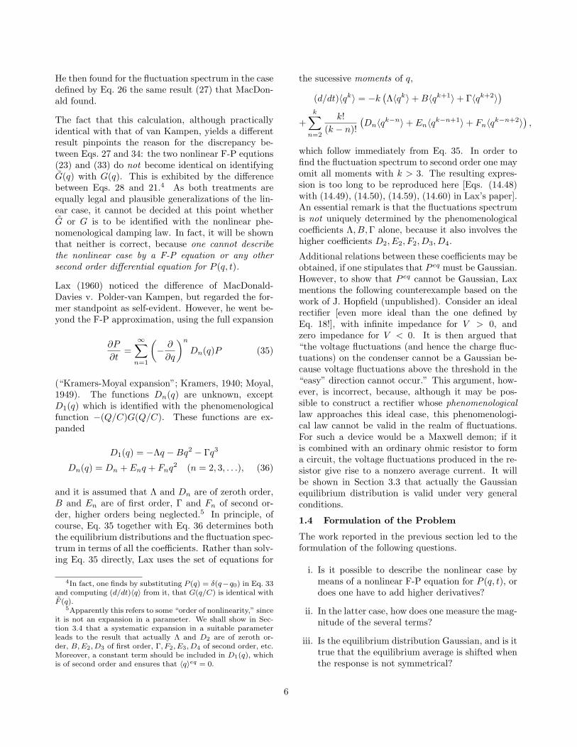
Alkemade (1958) introduced the model of a circuitand a vacuum diode valve consisting of two planeparallel electrodes of different metals (Fig. 3). Thediode is idealized by assuming that the electrons inthe diode vacuum space do not interfere with eachother (no space charge) and that the transit time ofthe electrons is zero. The whole system is in equilib-rium with a temperature bath. The work functionsof both electrodes are supposed to be different, suchthat electrode 1 operates under saturation conditions,i.e., it emits electrons at a constant rate independentof the potential difference (Fig. 4). Then the chargeQ on the condenser obeys the same phenomenologicallaw as the metal-oxide rectifier, Eq. 29.

The two terms in Eq. 29 are interpreted respectivelyas the probabilities per unit time for an electron tojump from electrode 1 to 2, and for a jump from 2to 1. (This interpretation of the phenomenologicallaw as determining directly the microscopic transitionprobabilities again amounts to identifying G with G.)By a kinetic calculation Alkemade then determinesthe high frequency limit

Sq(ω) ' 2π

kTCγ0 =2π

I0e. (37)

[The value γ0 is taken from Eq. 30.] The same resultwas found by Lax (1960). It disagrees with the for-mula obtained by using the approach of MacDonald(1957), see Eq. 32,

Sq(ω) ' 2π

kTCγ0

(1− 3

4e2

kTC

),

and with the result that is obtained with van Kam-pen’s method,

Sq(ω) ' 2π

kTCγ0

(1 +

16

e2

kTC

).

It will be shown in Section 3.2 that Eq. 37 is rigorouslycorrect.

The theory of Alkemade’s diode has been further de-veloped by van Kampen (1960). Let N be the num-ber of excess electrons on the condenser plate con-nected with electrode 1, so that the voltage differenceis −eN/C. The probability per unit time for each ofthese electrons to jump to electrode 2 is some constantA. The probability for an electron on electrode 2 toleave it is A exp[(W1 −W2)/kT ], but the probabilitythat it leaves with sufficient kinetic energy to reach

7

electrode 1 is6

A exp[(

W1 −e2

2C(N + 1)2

)−

(W2 −

e2

2CN2

)1

kT

]= Aeξ−εN ,

where

ξ =W1 −W2

kT− e2

2kTC, ε =

e2

kTC. (38)

Consequently the probability distribution PN (t)obeys the equation

1A

dPN

dt= PN+1 − PN + eξe−ε(N−1)PN−1 − e−εNPN.

(39)

This equation completely governs the behavior of thesystem under consideration and it is called the masterequation (ME).

2.2 Conclusions from the model

First the equilibrium distribution can be found bysolving Eq. 39 with dPN/dt = 0. It is easily seenthat the following solution holds:

P eqN = const. exp

[−1

2εN2 +

W1 −W2

kTN

].

This is indeed Gaussian. The center is neither at〈N〉eq = 0, nor at 〈N〉eq = − 1

2 , but at 〈N〉 = NC ,where NC corresponds to the contact potential:

eNC/C = (W1 −W2)/e.

This answers question (iii). Marek (1959) has arguedthat the average voltage in equilibrium must vanish,because of the second law of thermodynamics. Forhis argument it is essential, however, that the twoelectrodes of the rectifier are made of the same metal,with another material in between, so that there areno contact potentials in the remaining circuit. Such adevice is not described by our master equation (39).

Next we shall find the relation between the phenom-enological law and the ME. One derives directly from39, putting q = e(N −NC),

d

dt〈q〉 = eA

[1−

⟨eeq/kTC

⟩eε/2

]. (40)

This differs from the phenomenological law (29) in tworespects. First there is the factor eε/2. This factor isvery near to 1 and unobservable in any actual exper-iment. Yet it is essential in a microscopic treatment

6This argument is due to Alkemade.

because it cancels the − 12 e in 〈q〉eq [Eq. 31]. Note

that the function G, defined in Eq. 22, is, accordingto Eq. 40, given by

(q/C)G(q) = eA[1− eeq/kTCeε/2

], (41)

so that it is incorrect to identify it with the phenom-enological G. In fact, Eq. 41 could not serve as aresponse function for the diode, as it is not a functionof V alone, but depends on C as well (through ε).

The second difference is that the right-handside of Eq. 40 contains 〈exp[eq/kTC]〉 instead ofexp[e 〈q〉 /kTC]. The latter would be in accordancewith MacDonald’s general hypothesis, Eq. 15. Thefact that the former appears has profound conse-quences. It is easily seen, on expanding in the sameway as in Eq. 28, that the right-hand side does notdepend on 〈q〉 alone, but also on the higher moments〈(q − 〈q〉)2〉, etc. Hence, Eq. 40 is not at all a dif-ferential equation from which 〈q〉 can be solved as afunction of time. In fact, one should not expect thatthe infinite set of differential equations (39) reducesto just a single equation for the average.

Nevertheless, it is possible to extract an equation for〈q〉 by a suitable limiting process. Indeed, let C →∞,keeping the voltage V = q/C fixed. Then eε/2 → 1and moreover, since the fluctuations in V are of orderC− 1

2 and hence tend to zero⟨eeq/kTC

⟩=

⟨eeV/kT

⟩→ ee〈V 〉/kT .

Thus one obtains the phenomenological law from theequation for 〈q〉 by going to the limit of infinite con-denser, keeping the voltage fixed.

In order to compute the fluctuation spectrum fromEq. 39 it is necessary to expand.7 The only availableparameter is again ε, that is, 1/C. However, as we arenow dealing with the equilibrium state, the voltage Vwill now be itself of order C− 1

2 , and q = −e(N −NC)of order C

12 . It is therefore convenient to introduce

the normalized variable x,

x = ε1/2(N −NC), PN (t) + ε1/2P (x, t).

Then the Kramers-Moyal expansion of the ME (39)reads

1A

∂P

∂t= ε1/2 ∂P

∂x+

ε

2∂2P

∂x2+

ε3/2

3!∂3P

∂x3+ . . . (42)

+e−ε/2

−ε1/2 ∂

∂x+

ε

2∂2

∂x2

e−ε1/2xP.

7It happens that for the diode the fluctuation spectrum canbe found exactly without expanding (van Kampen, 1961b), butthat will not be true for most other cases.

8

The terms of order ε1/2 cancel, so ∂P/∂t is of orderε, in agreement with the increase of relaxation timeas C increases. It is therefore convenient to introducethe normalized time variable τ = εAt. The equationsfor the moments are then found to be

(d/dτ) 〈x〉 = −〈x〉+ε1/2

2(⟨

x2⟩− 1

)+

ε

2

(〈x〉 − 1

3⟨x3

⟩)+ O

(ε3/2

)(d/dτ)

⟨x2

⟩= 2− 2

⟨x2

⟩+ ε1/2

(⟨x3

⟩− 2 〈x〉

)+ O (ε)

(d/dτ)⟨x3

⟩= −3

⟨x3

⟩+ 6 〈x〉+ O

(ε1/2

). (43)

It is again true that the equation for 〈x〉 involvesall higher moments, but they occur with successivelyhigher powers of ε. Consequently, it is possible toobtain a closed set of equations if one only wants toknow 〈x〉 to a certain order. Thus Eqs. 43 permit oneto compute the conditional average 〈x〉x0 to first or-der in ε. This leads to the autocorrelation functionand hence to the fluctuation spectrum

Sx(ω) = (44)

2π

[(1− ε)

ω2

(1− 12ε)2 + ω2

+ε

4ω2

1 + (ω/2)2

]+ O(ε2).

This answers question (vi). Compare the result withEq. 32, noting that in the present units kTC = γ0 = 1.The high-frequency limit agrees with Eq. 37, as itshould.

Clearly, question(iv) cannot be settled by studying aspecial model for which all coefficients in the equa-tion for P are known; it will be further discussed inSection 3.6.

2.3 Validity of the Fokker-Planck Equation

In order to assess the validity of the F-P equation, wewrite the expansion of Eq. 42 explicitly

∂P

∂τ=

∂

∂x

x− ε1/2

2(x2 − 1

)+

ε

6(x3 − 3x

)P

+∂2

∂x2

1− ε1/2

2x +

ε

4(x2 − 1

)P

+∂3

∂x3

ε

6x

P +ε

12∂4P

∂x4. (45)

The zero-order term constitutes the linear F-P equa-tion (14). To order ε1/2 the equation is a nonlinearF-P equation: the linear coefficient has been supple-mented with a quadratic term, and the constant co-efficient of the second derivative has become a lin-ear function. Note that in the former also a constant

M

V

m v

Figure 5: The Rayleigh particle.

term 12 ε1/2 has appeared, which was not present in

the phenomenological law (29) and which cancels theanomalous result of Eq. 31. To this order ε1/2, how-ever, there are no corrections yet to the fluctuationspectrum.

The first order in ε adds higher corrections to thesame coefficients, but at the same time it brings inhigher derivatives. This shows that it is inconsistentto use the F-P equation for the nonlinear case, as wasdone by MacDonald, van Kampen and Davies. It isalso inconsistent to write all higher derivatives, whileincluding the nonlinearity only to a certain order, aswas done by Lax. There is just one single parameterε, which determines both the amount of nonlinearityand the validity of the Fokker-Planck equation. Thisanswers questions (i) and (ii).

The mathematical proof of the Fokker-Planck equa-tion (Khintchine, 1933; Middleton, 1960) suggests itsvalidity for practically all Markov processes, apartfrom some rather unrestrictive additional assump-tions. Actually these assumptions are crucial: theyamount to postulating that the individual transitionsare infinitely small. In the case of the diode this canonly be achieved by taking C large, which at the sametime has the effect of destroying the influence of thenonlinearity on the fluctuations.

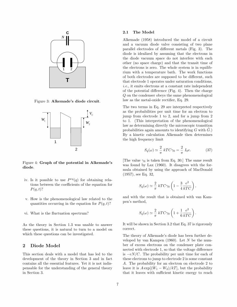
A similar situation prevails in the case of a Rayleighparticle. Rayleigh (1891; Zernike, 1929) studied theprobability distribution P (V, t) of one velocity com-ponent V of a heavy particle, mass M , immersed in agas of molecules of mass m (Fig. 5). It is convenientto picture the particle as a flat disc or piston. Theindividual transitions are due to collisions of the gasmolecules and are of order

∆V ∼ mv/M ∼ (m/M)(kT/m)1/2.

In equilibrium, V is of order V ∼ (kT/M)1/2, so thatthe F-P equation is a valid approximation if

1 ∆V/V ∼ (m/M)1/2. (46)

9

On the other hand, the damping law will be linearas long as V v; hence the equilibrium fluctuationsare not influenced b y the nonlinearity if V v, orM−1/2 m−1/2. Again this is the same condition asEq. 46. The purpose of the next chapter is to showthat this state of affairs is general, but two qualifyingremarks must be made.

First, for the purpose of finding the phenomenolog-ical law, the nonlinear F-P equation may be used,provided that the fluctuations are neglected. Indeed,the nonlinear F-P equation is obtained by erasing thethird and higher derivatives in the Kramers-Moyal ex-pansion (42). Obviously these terms do not contributeto (d/dt)〈x〉. Hence the nonlinear F-P equation leadsto the exact result (40), which reduces to the phenom-enological law in the limit in which the fluctuationsare neglected. This remark justifies the use of the non-linear F-P equation for deriving nonlinear generaliza-tions of Onsager’s reciprocal relations (van Kampen,1957; Uhlhorn, 1960).

Secondly, for the purpose of computing the fluctua-tion spectrum the nonlinear F-P equation is slightlybetter than would appear from the above criticism.The spectrum to order ε only requires 〈x〉 to orderε, and therefore 〈x2〉 to order ε1/2 and 〈x3〉 to orderε0. The third and higher derivatives in Eq. 42 do notaffect the first two moments, and contribute to 〈x3〉only in order ε1/2. Thus the nonlinear F-P equationstill gives the correct fluctuation spectrum to order ε;but for the terms of order ε2, the higher derivativesare indispensable.

3 General Theory

3.1 Statistical Foundations

We are concerned with systems that consist of a verylarge number N of particles. In classical theory, theprecise microscopic state of the system is describedby 6N variables x1, . . . , x3N , p1, . . . , p 3N . They obeythe 6N microscopic equations of motion. The gross,macroscopic aspect of the state is described by a muchsmaller number of variables Q1, . . . , Qn, which arefunctions of x1, . . . , p 3N . For convenience we supposethat apart from the energy there is just one other Q,and drop the label. Experience tells us the remarkablefact that this macroscopic variable Q (x1, . . . , p 3N )obeys again a differential equation

Q = F (Q), (47)

which permits to uniquely determine its future val-ues from its value at some initial instant. The phe-nomenological law (47) is not a purely mathematical

consequence of the microscopic equations of motion.The reason why it exists can be roughly understoodas follows. Using the equations of motion one has

Q =3N∑k=1

(∂Q

∂xkxk +

∂Q

∂pkpk

)≡ g (x1, . . . , p 3N ) .

The variables in g may be expressed in Q and theenergy (which we do not write explicitly), and 6N −2remaining variables, ϑλ (x1, . . . , p 3N ) say. Hence

Q = f (Q;ϑ1, . . . , ϑ 6N−2) .

This may also be written

Q(t + ∆t)−Q(t) =∫ t+∆t

t

f [Q(t′);ϑ(t′)] dt′.

Now suppose that Q(t) varies much more slowly thanthe ϑλ (which is the reason it is microscopic). It isthen possible to pick ∆t such that Q(t) does not varymuch during ∆t, while the ϑλ practically run throughall their possible values (ergodic theorem with fixedvalue for Q). Hence one may substitute in the inte-gral Q(t) for Q(t′) and replace the time integrationby an average over that part of the phase space thatcorresponds to given values of the energy and Q:

Q(t + ∆t)−Q(t) = ∆t · 〈f [Q(t);ϑ]〉Q(t) = ∆t · F [Q(t)].

It should be emphasized that this implies that at eachtime t the ϑλ vary in a sufficiently random way tojustify the use of a phase space average (“repeatedrandomness assumption”).

Fluctuations arise form the fact that, in the relevantpart of phase space, f is not exactly equal to its av-erage F , but has a probability distribution around it.Hence Q(t + ∆t) is no longer uniquely determined byQ(t), but instead there exists a transition probabilityW (q′|q). More precisely, ∆t W (q′|q) dq′ is the proba-bility that, if Q has the value q at time t, the value ofQ(t + ∆t) will lie between q′ and q′ + dq′. The prob-ability distribution P (q, t) of Q at any time t thenobeys the rate equation

∂P (q, t)∂t

=∫W (q|q′)P (q′, t)−W (q′|q)P (q, t)dq′.

(48)

This is the general form of the master equation, ofwhich Eq. 39 is a special case. It can also be derivedin quantum mechanics by an essentially similar argu-ment (van Kampen, 1954, 1956, 1962; van Hove, 1955,1962; Prigogine, 1962). Again a repeated randomness

10

T

ρ, NΩ

Figure 6: Density fluctuations in the volume Ω.

assumption is involved, namely that at each time theϑλ are sufficiently random to justify the identificationof probability with measure in phase space.

A formally equivalent way of writing the ME is ob-tained by expanding in powers of q′ − q,

∂P (q, t)∂t

=∞∑

n=1

1n!

(− ∂

∂q

)n

αn(q)P (q, t), (49)

where αn(q) are the successive moments of the tran-sition probability, or “derivate moments,”

αn(q) =∫

(q′ − q)nW (q′|q)dq′.

They are identical with the Dn(q) in Eq. 35 apartfrom a factor n!.

EXAMPLE 1. Alkemade’s diode (cf. Section 2.1 andFigs. 3 and 4). The macroscopic variable Q is thecharge on the condenser, or the number N of excesselectrons on one condenser plate. The remaining vari-ables ϑλ are all other quantities needed to specify themicroscopic state of the electrons and the heat bath.The transition probability is, according to Eq. 39,

W (N ′|N) = AδN ′,N−1 + Aeξ−εNδN ′,N+1. (50)

EXAMPLE 2. Density fluctuations. A box of vol-ume Ω communicates through a small hole with a verylarge volume, filled with a dilute gas with density ρ(Fig 6). For Q we take the number N of moleculesin Ω, while the remaining set of variables ϑ consistsof all momenta of the molecules and practically allof their coordinates, restricted only by the conditionthat exactly N of them must be in Ω. It is easily seenthat the procedure described above leads to the ME(with suitably chosen time unit)

∂P (N)∂t

=N + 1

ΩP (N + 1)− N

ΩP (N)

+ρP (N − 1)− P (N). (51)

EXAMPLE 3. Rayleigh’s piston (cf. Section 2.3 andFig. 5). There are two macroscopic variables, namelythe coordinate and the velocity of the heavy parti-cle; the coordinates and momenta of the gas particlesare the variables ϑλ. Of the two phenomenologicalequations, the one connecting the coordinate with thevelocity is trivial. The other one is the phenomenolog-ical damping law for the velocity and does not involvethe coordinates. In order to describe the fluctuationsit is replaced by a ME, the transition probability be-ing

W (V ′|V ) = nA

(M + m

2m

)2

|V ′ − V |×

f

(M + m

2mV ′ − M −m

2mV

). (52)

Here n is the number of molecules per cm3, f is theirvelocity distribution, A the surface area of the piston.

EXAMPLE 4. Brownian particle. The same particlestudied on a longer time scale, so that the instanta-neous velocity is not observed. The macroscopic vari-able is the coordinate, while the ϑλ now also includethe velocity of the heavy particle. The right-hand sideof Eq. 47 is now zero, the displacement of the parti-cle is wholly due to fluctuations. Kramers (1940) hasgiven a general treatment, which comprises both theRayleigh and Brownian aspect.

EXAMPLE 5. n-type semiconductor. The macro-scopic variable is the number N of electrons in theconduction band, the ϑλ are all other variables. Thetransition probability has the form (Burgess, 1955a,b,1956; van der Ziel, 1959)

W (N ′|N) = r(N)δN ′,N−1 + g(N)δN ′,N+1, (53)

where r(N) and g(N) are linear or quadratic func-tions of N , depending on the kind of semiconductorconsidered. In particular, for the strongly extrinsicsemiconductor

r(N) = r0ω

(N

Ω

)2

, g(N) = g0ω

(nd −

N

Ω

)(54)

where r0 and g0 are constants, Ω the volume, nd thenumber of donors per unit volume.

3.2 General Properties of the Master Equa-tion

The master equation (48) is of the form

P = WP, (55)

11

where W is a linear operator acting on functions of q.Equations of this form occur in many parts of physics:diffusion, heat conduction, Schrodinger equation, Li-ouville equation, etc. For the familiar mathematicaltechniques of eigenvalues and eigenfunctions, however,it is essential that W be a symmetrical or self-adjointoperator.Fortunately, the transition probabilities havethe property of reciprocity, which is almost as good.

To formulate reciprocity, one must distinguish be-tween even and odd macroscopic variables. Q is aidto be even when it is an even function of all velocities,so that its value remains the same if the microscopicmotion of all particles is reversed. It is an odd vari-able when it changes sign on reversing motion. Inthe third example above, V is an odd variable, in theother examples the macroscopic variables are even.

Both when Q is even and when Q is odd on hasP eq(q) = P eq(−q). When Q is even, reciprocity states

W (q′|q)P eq(q) = W (q|q′)P eq(q′), (56)

which is also called “microscopic reversibility” or “de-tailed balance,” and can be proved generally (Wigner,1954; van Kampen, 1954). It is convenient to define a“scalar product” of any two functions P1(q) and P2(q)by

(P1, P2) =∫

P1(q)P2(q)dq

P eq(q), (57)

so that Eq. 56 can be expressed by

(P1,WP2) = (P2,WP1) = (WP1, P2), (58)

which states that W is self-adjoint. In addition,one may deduce from Eq. 56 and the fact thatW (q|q′) ≥ 0,

(P,WP ) ≤ 0. (59)

More generally, let f(x) be an concave function [i.e.,f ′′(x) ≥ 0]; then it can be shown in the same way that

H =∫

P eqf(P/P eq)dq

never increases. Particular choices are

H =∫

P log(P/P eq)dq and

H =∫

(P 2/P eq)dq; (60)

the former is minus the Gibbs entropy and the latterwill used in Section 3.5.

By setting P (q, t) = eλtPλ(q), Eq. 55 is reduced tothe eigenvalue problem

WPλ = −λPλ. (61)

The eigenfunctions Pλ are mutually orthogonal interms of the scalar product (57). Because of Eq. 59one has λ ≥ 0. There is an eigenvalue λ = 0with eigenfunction P0(q) ≡ P eq(q). It may be as-sumed that this eigenvalue is not degenerate becauseit can be shown that otherwise W is reducible, sothat the ME decomposes into a number of separatemaster equations. For convenience, we also assumethat the eigenvalues are discrete; in some cases (dif-fusion, Brownian movement), the spectrum is contin-uous, which requires only minor modifications.

If one has a complete set of eigenfunctions Pλ, nor-malized to (Pλ, Pλ) = 1, the completeness relation∑

λ

Pλ(q)Pλ(q′) = P eq(q) · δ(q − q′)

holds. Consequently, the solution of the ME that re-duces to δ(q − q0) for t = 0 is

Pt(q|q0) =∑

λ

e−λtPλ(q)Pλ(q0)/P eq(q0). (62)

This is the transition probability from q0 to q in timet. Hence the autocorrelation function is

〈q0〈q(t)〉q0〉eq =∫

P eq(q0)q0 dq0

∫Pt(q0|q)q dq

=∑

λ

e−λt

[∫Pλ(q)q dq

]2

. (63)

The fluctuation spectrum of q is therefore

Sq(ω) =2π

∑λ

λ

λ2 + ω2

[∫Pλ(q)q dq

]2

. (64)

An asymptotic expression for high frequencies is ob-tained by expanding each term in 1/ω2:

Sq(ω) ' 2π

∞∑n=0

(− 1

ω2

)n+1

〈qW2n+1q〉eq,

where W is the transposed operator of W, defined by∫f(q)Wg(q)dq =

∫g(q)Wf(q)dq,

for any f and g. In particular, one has

limω→∞

Sq(ω) = − 2π〈qWq〉eq.

12

Inserting W from Eq. 50, one obtains Alkemade’s re-sult (37).

When Q is an odd variable, reciprocity consists of twoequations

W (q′|q)P eq(q) = W (−q| − q′)P eq(q′),∫W (q′|q) dq′ =

∫W (−q′| − q) dq′.

Whether the previous work can be extended to thiscase has not been fully investigated. However, in somesimple cases, like the Rayleigh particle, W also obeysEqs. 58 and 59, even though the variable is odd, sothat the previous work applies.

3.3 The Equilibrium Distribution

When derivingEq. 56, the function P eq(q) enters as avolume of phase space; it is then found a posteriorifrom Eq. 56 that P eq(q) is indeed a time-independentsolution of the ME (48). The explicit form of P eq(q) isa matter of equilibrium statistical mechanics. In thelinear theory, P eq(q) is always taken to be a Gaussian.As mentioned in Section 1.3, MacDonald (1957) raisedthe question whether this is still correct in the pres-ence of nonlinearity. Indeed, that this cannot alwaysbe correct is obvious from the example of the densityfluctuations, for the equilibrium distribution must bea Poisson function, as is easily verified from Eq. 51.On the other hand, the examples of the diode andthe Rayleigh particle demonstrate that a nonlinearphenomenological law is not necessarily incompatiblewith a Gaussian equilibrium distribution. The follow-ing theorem seems to cover most cases.

The equilibrium distribution is a Gaussian function ofthe microscopic variable q if

i. the energy of the total system is quadratic in q;and

ii. the interaction (i.e., that part of the total Hamil-tonian of the system that is responsible for transi-tions between different values of q) has a strengthparameter which enters W (q|q′) as a factor thatpermits one to scale down the magnitude ofW (q|q′) without affecting its functional depen-dence on q and q′.

Condition (i) ensures that, according to equilibriumstatistical mechanics

P eq(q) ∝ exp(−cq2). (65)

This condition rules out the case of the density fluc-tuations. The second condition is necessary as Eq. 65

is only exact for infinitely small interaction. Thestrength parameter permits one to go to this limit,without altering the form of P eq. Hence, Eq. 65 mustbe exact for all values of the strength parameter be-cause P eq(q) does not depend on the magnitude ofW (q|q′), but only on its functional dependence on qand q′.

Both conditions are fulfilled for the diode model, thestrength parameter being the surface area of the elec-trodes; and for the Rayleigh piston, the strength pa-rameter being the area A of the piston.

3.4 Power Series Expansion of the MasterEquation

The ME can be solved exactly for the example of den-sity fluctuations, Eq. 51, and for the example of thediode, Eq. 39 (van Kampen, 1961b). In most othercases an approximation method has to be used.In or-der to avoid the ambiguities reported in Section 1.3,it is essential to use a systematic expansion, like inSection 2.2. To find a suitable expansion parameter,analogous to ε = e2/kTC in Section 2.2, we note: (i)the magnitude of the fluctuations is usually given interms of an extensive quantity, like charge or num-ber of particles; (ii) the dependence of the transitionprobability is properly expressed through an intensivequantity, like voltage or particle density. Supposingq to denote an extensive quantity, we introduce thecorresponding intensive quantity X = q/Ω, where Ωis some measure for the size of the system. It is thennatural to write for the transition probability

W (q′|q) = Φ( q

Ω; q′ − q

)= Φ(X; q′ − q). (66)

We expect that Φ, in contrast to W , no longer de-pends implicitly on Ω. This is indeed for density fluc-tuations, Eq. 51; and for the Rayleigh particle, Eq. 52,on putting

X = V, q =M + m

mV, Ω =

M + m

m. (67)

It is also true for the strongly extrinsic semiconductordescribed by Eqs. 53 and 54, except for a factor Ω in Φ,which can easily be removed by a change in time scale.It is clear from Eq. 66 that Ω measures the relativemagnitude of the fluctuations: as Ω →∞, the fluctu-ations in X tend to zero, so that they can be madesmall compared to the range over which the phenom-enological function G(X) varies materially. Therefore,we shall expand in reciprocal powers of Ω.

For this purpose we make all powers of Ω explicit by

13

the following transformation of variables,

t = Ωτ (68)

q = Ωϕ(τ) + Ω1/2x, q′ = q + ∆q, (69)

P (q, t) = P (Ωϕ(τ) + Ω1/2x,Ωτ) ≡ Π(x, τ). (70)

Equation (68) takes account of the increasing relax-ation time.8 Equation (69) expresses that q consistsof two parts: the macroscopic part Ωϕ(τ), whose de-pendence on time is described by ϕ(τ) and will bedetermined presently; and a fluctuating part, whichwill be of order Ω1/2. When this is substituted inEq. 49, the expansion in Ω is straightforward. Wewrite α

(p)n (X) for the pth derivative with respect to

X of the derivate moment αn. One finds after somemanipulations (van Kampen, 1961a)

∂Π∂τ

− Ω1/2ϕ′(τ)∂Π∂x

= −Ω1/2α1ϕ(τ)∂Π∂x

(71)

+∞∑

m=2

Ω−12 (m−2)

m!

m∑n=1

(m

n

)α(m−n)

n ϕ(τ)(−∂

∂x

)n

xm−nΠ.

First, equating the terms of order Ω1/2, one finds thephenomenological law

dϕ

dτ= α1(ϕ), or

dq

dt= α1(X). (72)

This determines ϕ(τ) for any given initial value ϕ(0).Inserting this result in (71), one obtains an equationfor the probability distribution Π(x, τ) of the fluctu-ations around the macroscopic value. The two lowestorders are

∂Π∂τ

= − ∂

∂x

[α

(1)1 x +

12Ω−1/2α

(2)1 x2 + . . .

]Π

+12

∂2

∂x2

[α

(0)2 + Ω−1/2α

(1)2 x + . . .

]Π

− 13!

∂3

∂x3

[Ω−1/2α

(0)3 + . . .

]Π. (73)

All α(p)n are to be taken at ϕ(τ), or, if one is inter-

ested in equilibrium fluctuations, at ϕ(∞). The twozero order terms constitute the linear Fokker-Planckequation (14). The next order corrects the coefficientsof both terms, and adds a third derivative. Similarly,each higher order of Ω−1/2 adds one higher derivative.Hence the result found in Section 2.2 for the diode isgeneral: It is inconsistent to use the F-P equation

8This transformation is not required when the fluctuationsare a bulk property, as for chemical reactions or for carrierfluctuations in semiconductors [cf. Eq. 54]

for the nonlinear case, but it is equally inconsistentto add higher derivatives without at the same timecorrecting the coefficients of the lower derivatives.

Additional remark. In the case of the Rayleigh par-ticle it is customary to expand in m/M rather thanin m/(M + m). This amounts to putting, instead ofEq. 67,

X = V, q = MV/m, Ω = M/m.

In that case, Φ is not independent of Ω, see Eqs. 52and 66. In more elaborate examples, this is evenunavoidable, for instance if the Rayleigh particle isimersed in a mixture of gases (Alkemade et al., 1963).However, that does not invalidate the above expan-sion method because it is still true that Φ is a powerseries in 1/Ω. The only consequence is that the αn

are also power series in 1/Ω,

αn(X) = αn,0(X) + Ω−1αn,1(X) + . . . . (74)

It is then consistent to identify the phenomenologicallaw not with Eq. 72, but with its lowest order,

dq/dt = α1,0(X).

The terms with α1,1(X), etc., are to be included inthe equation (73) for Π.9 Moreover, the α

(p)n in (73)

involve higher powers of 1/Ω, which should only beincluded as far as necessary.

3.5 Siegel’s Expansion

The ME (55) has the essential property that W is“negative semi-definite” in the sense that it has oneeigenvalue λ = 0 with eigenfunction P eq, all othereigenvalues being negative. This property guaranteesthat every solution tends to P eq for t → ∞. Thesuccessive approximations in the expansion of Sec-tion 3.4, however, do not all have this property. Siegel(1960) has shown that this can be remedied by the fol-lowing procedure.

As −W is positive semidefinite, it has a square rootU, in the sense that

−W = UU = U2,

where U is another self-adjoint operator.10 In factone readily verifies

U(q|q′) =∑

q

√λPλ(q)Pλ(q′)/P eq(q′). (75)

9This also occurs in the diode; for instance the terms 12ε1/2

and − 12εx on the first line of Eq. 45 are of this nature.

10Actually Siegel writes W = −UU†, so that U need not beself-adjoint.

14

Now suppose W has been expanded in Ω−1/2, to sec-ond order, say. One may then also write for U aquadratic expression in Ω−1/2 and determine the co-efficients U0,U1,U2, successively, from the require-ment

−(U0 + Ω−1/2U1 + Ω−1U2)2 = W + O(Ω−3/2).

the left-hand side is then a correct approximation tosecond order, and self-adjoint and negative semidefi-nite by construction, thanks to the addition of someterms of higher order.

In the second part of his paper, Siegel gives the fol-lowing expansion for the operator W.11 It is assumedthat P eq(q) is Gaussian and is given by Eq. 65 withc = 1

2 . We start from the ME in the form (49) andexpand the αn(q) in Hermite polynomials

αn(q) =∞∑

k=0

αnkHk(q), Hk(q) = e12 q2

(− d

dq

)n

e−12 q2

.

One then has

∂P

∂t= e−

12 q2 ∑

n,k

αnk

n!

(q

2− ∂

∂q

)n

Hk(q)e12 q2

P.

We substitute the mathematical identity

Hk(q) =k∑

l=0

(k

l

) (q

2− d

dq

)k−l (q

2+

d

dq

)l

,

and obtain after some rearrangements Siegel’s expan-sion

∂P

∂t= (76)

e−12 q2

∞∑m=0

m∑l=0

Alm

(q

2− ∂

∂q

)k−l (q

2+

∂

∂q

)l

e12 q2

P,

where

Alm =1√2π

1l!

m∑k=l

∫∞−∞ αm−k+1(q)Hk(q)e−

12 q2

dq

(k − l)!(m− k + 1)!.

From the fact that e−q2/2 must obey Eq. 76, it followsthat all A0m must vanish. The first non-vanishingterm, with m = 1, l = 1, is just the linear F-P equa-tion. For self-adjointness, one must have Al,m =Am−l+1,m, which implies a property of the αn,k, butthis has not been investigated.

11The present derivation is somewhat different from the orig-inal one.

Equation (76) is not a power series expansion in a pa-rameter. Siegel suggests that the magnitude of thesuccessive terms with m = 1, 2, . . . should be esti-mated from their contributions to dH/dt, where His taken from the second expression in Eq. 60. Inthe spirit of Section 3.4, however, it can also be veri-fied that Alm is of order Ω−m/2, although it includeshigher orders, too. In addition, when breaking off ata certain m, the operator must still be made negativesemidefinite by applying the above-mentioned proce-dure.

After constructing in this way an approximate W,which is self-adjoint, negative semidefinite, and cor-rect to some order Ω−m/2, one may compute fromit the fluctuation spectrum to that same order, forinstance, by means of Eq. 64. The result is identi-cal with the one obtained in a less laborious way bymean of the expansion (73). However, in the lattercase Eq. 64 is unsuitable because some of the eigenval-ues λ may turn out positive or complex, since Eq. 73is not self-adjoint and negative definite in each or-der. Instead, one must treat the higher order terms inEq. 73 as perturbations of the linear F-P equation.12

3.6 The Connection between Fluctuationsand Dissipation

In the linear theory of Section 1.2, the fluctuationspectrum of q was calculated from Eqs. 4 and 5, with-out using Eq. 6. The fluctuation spectrum of κ is thenalso known:

Sκ(ω) = (γ20 + ω2)Sq(ω)

= (2/π)γ0〈q2〉eq = (2/π)kTCγ0.

This agrees with the autocorrelation function (6), pro-vided that

Γ = 2kTCγ0 = 2kT/R. (77)

This is called the Nyquist relation (Nyquist, 1928),and is closely related to Einstein’s relation for Brown-ian movement (Einstein, 1905, 1906). It connectsa stochastic property of the electromotive force pro-duced in the resistor with its dissipative property. Thesame relation is found in the Fokker-Planck approachby adjusting Γ in Eq. 14, so as to obtain the correctequilibrium distribution.

12An analogous situation prevails in the quantum mechani-cal calculation of the Stark effect. The exact Hamiltonian of anatom in an electric field has no discrete eigenvalues. Yet pertur-bation theory gives the correct shifts of the discrete eigenvaluesof the unperturbed Hamiltonian.

15

One has to know Γ for calculating 〈q2(t)〉 from a giveninitial 〈q(0)〉. In fact, Eq. 77 is usually derived by do-ing just this and then using the fact that q2(t) shouldtend to 〈q2〉eq = kTC as t →∞ (Uhlenbeck and Orn-stein, 1930). Thus the Nyquist theorem implies that,for linear systems, the mean square of the fluctuationscan be found as a function of time from the macro-scopic damping constant alone, without knowing any-thing about the detailed mechanism that causes thefluctuations. The higher moments, like 〈q4(t)〉, how-ever, involve higher moments of κ(t), like

〈κ(t)κ(t′)κ(t′′)κ(t′′′)〉,

and cannot therefore be found without knowing moreabout this fluctuating force.13

The question of how to extend the Nyquist relationto nonlinear systems may be formulated as follows.The equilibrium fluctuations are described by Eq. 73,the coefficients α

(p)n all being taken at the equilibrium

value ϕ(∞), so that they are constant. The macro-scopic dissipation is, according to Eq. 72, describedby the phenomenological law α1(X), which involvesthe constants α

(p)1 . Which relations, independent of

the detailed mechanism, exist that relate the α(p)n for

n > 1 to α(p)1 ? [This formulation only applies if the

αn(X) are independent of Ω. If they contain alsohigher powers of Ω−1 (see Eq. 74), the question is:Which relations exist relating the α

(p)n,ν for n > 1 and

the α(p)1,ν for ν > 0 to the phenomenological coefficients

α(p)1,0?]

Since this question has not been fully solved we shallonly make some remarks. First, one knows thatΠeq(x) = const. exp

(− 1

2x2)

must be a solution toeach order of Ω. By substituting this solution inEq. 73, one obtains a relation between the coefficientsof each separate order of Ω. In particular, the orderΩ0 yields α

(0)2 = −2α

(1)1 , which is the familiar Nyquist

relation (77). Secondly, it is possible to obtain addi-tional relations by using the reciprocity relation (56).It has been shown for a generalized Rayleigh model(a piston between two different arbitrary mixtures of

13It may seem that the F-P equation (14) is superior in thisrespect to the Langevin equation, because it does not permitone to compute higher moments. The fact is, however, thatsome specific assumptions have been incorporated in Eq. 14 byomitting the higher derivatives. These assumptions correspondto a set of specific assumptions concerning the stochastic behav-ior of κ(t); they may be written in condensed form as follows:

exp

Z t

0κ(t′)dt′

= exp

1

2Γt

.

gases) that in this way all coefficients up to orderΩ−1/2 are uniquely determined in terms of the co-efficients α′1,0 and α′′1,0 of the phenomenological law(Alkemade et al., 1963). This is no longer true for thecoefficients of the terms of order Ω−1.

4 Microscopic Theories

Section 3 was based on the master equation (48),which can be derived from the microscopic equationsof motion (either classical or quantum-mechanical) atthe expense of a repeated randomness assumption (cf.Section 3.1). In the present Section 4 we discuss theattempts that have been made to derive the propertiesof nonlinear fluctuations directly from the microscopicequations. The author believes that this easily leadsto an erroneous identification of microscopic expres-sions with phenomenologically observed quantities, aswill be pointed out in connection with the Nyquist re-lation for nonlinear systems.

4.1 Classical Theory

Let X denote a point in 6N -dimensional phase space,H(X) the Hamiltonian function of the isolated sys-tem, and ρ(X) a probability density describing thestate of an ensemble at t = 0. The probability forsome physical quantity Q(X) to lie between q andq + dq is

P (q, 0)dq = dq

∫δQ(X)− qρ(X)dX.

After a time t, the motion in phase space has carriedX to a new point Xt, so that

P (q, t) =∫

δQ(Xt)− qρ(X)dX.

Equilibrium is described by

ρeq(X) = Z−1e−βH(X), Z =∫

e−βH(X)dX.

The autocorrelation function of equilibrium fluctua-tions is∫

Q(X)Q(Xt)ρeq(X)dX − ∫

Q(X)ρeq(X)dX2.

(78)

A state in which the quantity Q is known to have thevalue q0 is described by

ρq0(X) = Z−1q0

e−βH(X)δQ(X)− q0, (79)

16

where the normalizing factor is easily seen to be Zq0 =ZP eq(q0). The transition probability in time t is

Pt(q|q0) =∫

δQ(Xt)− qρq0(X)dX. (80)

In a series of papaers, Magalinskii and Terletskii(1958, 1959, 1960; Terletskii, 1958; Magalinskii, 1959)have developed this formalism. On substitutingEq. 79 in Eq. 80 and replacing the δ-functions withtheir Fourier integrals, they obtain

Pt(q|q0)P eq(q0) =

(2π)−2Z−1

∫ ∫exp[iξq + iξ0q0]Mt(ξ|ξ0)dξdξ0,

Mt(ξ|xi0) =∫

exp[−iξQ(Xt)− iξ0Q(X)]e−βH(X)dX.

This function Mt(ξ|ξ0) contains all information con-cerning the quantity Q; e.g., the autocorrelation func-tion (78) is

〈QQ(t)〉eq − 〈Q〉eq = −[∂2 log Mt(ξ|ξ0)

∂ξ∂ξ0

]ξ=ξ0=0

.

(81)

One may also verify

〈Q(t)〉q0 =∫

Q(Xt)ρq0(X)dX (82)

=[i

∂

∂ξlog

∫exp[iξ0q0]Mt(ξ|ξ0)dξ0

]ξ0=0

.

Equation (80) describes an ensemble for which Q hasthe precise value q0 with no fluctuations around it. Ifit is only known that the average value 〈Q〉 equals q0,other choices are possible. In the spirit of Gibbs, it isnatural to choose

ρα0(X) = Z(α0)−1 exp[−βH(X)− α0Q(X)],

Z(α0) =∫

exp[−βH(X)− α0Q(X)]dX, (83)

where α0 is an auxiliary parameter, to be determinedfrom

q0 =∫

Q(X)ρα0(X)dX = −∂ log Z(α0)∂α0

.

Alternatively, one may regard ρα0(X) as theequilibrium distribution for a new HamiltonianH ′ = H + (α0/β)Q. This amy be interpreted as theaddition of an external force F = α/β acting on the

coordinate Q. Hence, if the system has reached equi-librium under the influence of this constant force, andif this force is suddenly switched off at t = 0,

〈Q(t > 0)〉α0 =∫

Q(Xt)ρα0(X)dX

=[i∂ log Mt(ξ| − iα0)

∂ξ

]ξ=0

. (84)

The fact that this differs from Eq. 4.1 clearly showsthat the value of 〈Q〉t not only depends on the initialaverage 〈Q〉0, but is also influenced by the fluctuationsin the initial state.

If one disregards this influence, and (arbitrarily) iden-tifies Eq. 84 with the phenomenological behavior, onearrives at an expression for ∂ log Mt/∂ξ as a functionof α0 and hence of ξ0, but only at ξ = 0. In orderto extend this to other values of ξ, Magalinskii andTerletskii introduce

Mt(ξ − iα|ξ0 − iα0) =∫

exp[−iξQ(Xt)− iξ0Q(X)]×

× exp[−βH(X)− α0Q(X)− α0Q(Xt)]dX,

and assert that this describes the behavior of a systemthat at t = 0 has reached equilibrium under the influ-ence of the external force (α0+α)/β, which at t = 0 issuddenly reduced to α/β. This is incorrect, however,because the external force α/β should also affect theconnection between Xt and X. Indeed, the knowledgeof Mt(ξ|ξ0) is equivalent to a complete solution of themicroscopic equations of motion; one cannot hope tofind it from phenomenological data alone.

A correct relation has been obtained by Vladimirskii(1942). By differentiating Eq. 84, and comparing theresult with Eq. 81, one has

−[

∂

∂α0〈Q(t)〉α0

]α0=0

= −[∂2 log Mt(ξ|ξ0)

∂ξ∂ξ0

]ξ=ξ0=0

〈QQ(t)〉eq − (〈Q〉eq)2. (85)

This constitutes an exact relationship between dissi-pation and equilibrium fluctuations. The dissipativeterm on the left, however, should be carefully inter-preted. It is the difference between 〈Q(t)〉 measuredfor two differently prepared systems: one being inequilibrium at all times, the other having been uptill t = 0 in equilibrium subject to an infinitesimalexternal force F = α0/β, which is then switched off.

4.2 The Quantum Mechanical Theory ofBernard and Callen

Let H be the Hamiltonian of a closed, isolatedsystem, Z = Tre−βH its partition function, and

17

ρeq = Z−1e−βH the density matrix describing equi-librium. If Q is the operator associated with a certainphysical quantity in the Schrodinger representation,then variation of this quantity in time is described bythe Heisenberg operator

Q(t) = eitHQe−itH (~ = 1). (86)

It is natural to take as a quantum mechanical versionof the autocorrelation function (7)

12〈QQ(t) + Q(t)Q〉eq =

12TrρeqQQ(t) + Q(t)Q.

(87)

If the subscripts k, l, . . . denote the various eigenstatesof the exact Hamiltonian H, and Ek its eigenvalues,the expression (87) may be written

12Z−1

∑k,l

e−βEkQklQlkeit(El−Ek) + e−it(El−Ek).

The spectral density of the fluctuations is, accordingto the Wiener-Khintchine theorem (10),

SQ(ω) = Z−1∑k,l

e−βEk |Qkl|2×

×δ(Ek − El + ω) + δ(Ek − El − ω).

By interchanging the subscripts k and l in the secondterm, one obtains

SQ(ω) = Z−1(1 + e−βω)∑k,l

e−βEk |Qkl|2δ(Ek − El + ω).

(88)

It is less clear how the phenomenological law is con-nected with the microscopic quantum mechanical for-malism. We shall here describe the method of Bernardand Callen (1959). Let F be an external force actingon Q, such that the Hamiltonian is H + FQ. It isargued that F may be regarded as a known complexnumber depending on time. The density matrix ρ(t)obeys the equation

iρ = [H, ρ] + F (t)[Q, ρ]. (89)

One splits off the unperturbed part of ρ, putting

ρ = ρeq + e−itHσeitH ,

so that

iσ = F (t)[Q(t), ρeq] + O(F 2).

Supposing that at t = −∞ the system is in the un-perturbed equilibrium state described by ρeq, one hasto first order in F ,

σ(t) = −i

t∫−∞

F (t′)[Q(t′), ρeq]dt′. (90)

Hence, the expectation value of Q at time t is

〈Q〉t = 〈Q〉eq + i

t∫−∞

F (t′)dt′Trρeq[Q(t′), Q(t)]. (91)

Let the “aftereffect function” Φ(t2− t1) be defined fort2 ≥ t1 as the response 〈Q〉 at t2, provoked by a pulseF (t) = δ(t− t1). According to Eq. 91

Φ(t2 − t1) = iTrρeq[Q(t1)Q(t2)] = i〈[Q, Q(t2 − t1)]〉eq.

The response to the periodic force F (t) = eiωt is〈Q〉t − 〈Q〉eq = L(ω)e−ωt, where the “response func-tion” is

L(ω) =

∞∫0

Φ(t)eiωtdt. (92)

A similar calculation as used above yields

ImL(ω) = −πZ−1(1 + e−βω)×

×∑k,l

e−βEk |Qkl|2δ(Ek − El + ω).

Comparison with Eq. 88 leads to a relation betweenthis response function and the fluctuation spectrum:

SQ(ω) = − 1π

1 + e−βω

1− e−βωImL(ω). (93)

This is the “fluctuation-dissipation theorem” (Callenand Welton, 1951). As an example: when this rela-tion is applied to the electric circuit of Fig. 1 (withconstant resistance R), one has F = V/R, L(ω) =−R−1(−iω +1/RC)−1 so that one finds Eq. 11 as theclassical limit (βω 1).

Subsequently, Bernard and Callen proceed to the nextorder, which involves three effects.

i. The response (90) is supplemented by a term oforder F 2:

−t∫

−∞

F (t′)dt′t′∫

−∞

F (t′′)dt′′TrρeqQ(t′′), [Q(t′), Q(t)].

(94)

18

ii. In a stationary state with constant driving forceF , the fluctuation spectrum is no longer equal toEq. 88. The correction is now taken into accountto first order in F . It clearly involves productsof three factors Q and is therefore related to thedouble commutator in Eq. 94.

iii. Even in equilibrium, the autocorrelation function(88) is not an exhaustive description of the sto-chastic properties of the fluctuations; more infor-mation is contained in the higher moments. Thethird moment 〈QQ(t)Q(t′)symmetrized〉

eq be-longs to the same approximation as the aboveeffects (i) and (ii).

We shall not discuss these higher order terms, how-ever, because a serious difficulty appears already inEq. 93. This equation asserts that the fluctuationspectrum in equilibrium is completely determined bythe linear response alone, regardless of the existenceof nonlinear terms in the phenomenological response.This contradicts our previous results, in particularEq. 44, for the diode model. The point will be dis-cussed presently.

We stress the fundamental difference between the ap-proaches in this section and in the previous one. Theprevious section is based on the master equation (48),which describes the stochastic behavior of a macro-scopic variable. The stochastic character, togetherwith irreversibility, is due to the repeated averagingover all other microscopic variables, see Section 3.1.The present section is directly based on the micro-scopic equation of motion, without averaging over mi-croscopic variables.14 As a consequence, Eq. 91 ex-presses 〈Q〉t as an integral over the entire past of F (t).The system never forgets, because no irreversibilityhas entered the picture. This is clearly exhibited bythe fact that , in addition to Eq. 91, one has the an-ticausal equation

〈Q〉t = 〈Q〉eq − i

∞∫t

F (t′)dt′Trρeq[Q(t′), Q(t)],

if it supposed that the system is in equilibrium att = +∞. Accordingly Eq. 91 is of entirely differentnature than Eqs. 1 and 2, which express the rate ofchange of Q in terms of the instantaneous value of theforce.

14The density matrix implies an averaging over initial states,but that is a more elementary process, which does not sufficeto derive the ME.

In a second paper, Bernard and Callen (1960) sup-port their conclusion that the fluctuation spectrum isnot affected by nonlinear terms, without invoking themicroscopic equations. However, they here start fromEq. 15, which was shown by Polder to be untenable.This is related to the fact that the expression theyuse for the autocorrelation function is incorrect (vanKampen, 1960).

4.3 An Alternative Quantum MechanicalTreatment; Discussion

Stratonovich (1960) has quantized the theory of Ma-galinskii and Terletskii (Section 4.1); we merely re-produce the main results. A state given by 〈Q〉 isdescribed by the density matrix

ρα0Z(α0)−1 exp(−βH − α0Q),Z(α0) = Tr exp(−βH − α0Q), (95)

which is the quantum analog of Eq. 83. Let us intro-duce again the auxiliary function

Mt(ξ|ξ0) = Tr exp(−βH − iξ0Q)e−iξQ(t),

where Q(t) is the same as in Eq. 86. Then one has

〈Q(t)〉α0 = Trρα0Q(t) =[i∂ log Mt(ξ| − iα0)

∂ξ

]ξ=0

,

in complete analogy with Eq. 84.

In order to find the analog of Eq. 81, one needs theidentity

∂

∂ξ0exp(−βH − iξ0Q) =

−i

βe−βH

β∫0

eβ′HQe−β′Hdβ′ + O(ξ0).

It is then easy to compute

[∂2Mt(ξ|ξ0)

∂ξ∂ξ0

]ξ=ξ0=0

= − 1β

β∫0

dβ′Tre−βHQQ(t + iβ′).

Hence one finds, instead of the classical Eq. 81,

−[∂2 log Mt(ξ|ξ0)

∂ξ∂ξ0

]ξ=ξ0=0

=

=1β

β∫0

dβ′〈QQ(t + iβ′)〉eq − (〈Q〉eq)2

=(

iβd

dt

)−1 exp

[iβ

d

dt

]− 1

〈QQ(t)〉eq − (〈Q〉eq)2.

19

eqP0

Pα

q

Figure 7: The equilibrium distribution P eq, theshifted distribution Pα0 , and a distribution thatappears to a macroscopic observer as a non-equilibrium state.

Thus, the second derivative of Mt is no longer identi-cal with the autocorrelation function, but an operatorintervenes acting on the time dependency. Accord-ingly, one now obtains instead of Eq. 85

〈QQ(t)〉eq − (〈Q〉eq)2 =

=(

iβd

dt

) exp

[iβ

d

dt

]− 1

−1 [∂

∂α0〈Q(t)〉α0

].

The real part of this equation is (take 〈Q〉eq = 0 forbrevity)

12〈QQ(t) + Q(t)Q〉eq = (96)

= −(

β

2d

dt

)cot

(β

2d

dt

) [∂〈Q(t)〉α0

∂α0

]α0=0

.

To show that this result is identical with Eq. 93, wefirst note that 〈Q(t)〉α0 is the afetreffect of a constantforce F = α0/β, acting from t = −∞ till t = 0,

〈Q(t)〉α0 =

0∫−∞

Φ(t− t′)α0

βdt′ + O(α2

0).

Hence, [∂

∂α0〈Q(t)〉α0

]α0=0

=1β

∞∫t

Φ(t′)dt′.

Substitute this in Eq. 96, multiply with (2/π) cos ωt,integrate from −∞ to 0: the result is Eq. 93.

Equation (85), its quantum mechanical version (96),and the Fourier transform thereof, Eq. 93, are equiv-alent expressions of the relation between equilibriumfluctuations and the relaxation of 〈Q〉 after a weakforce has been applied. We shall argue that this re-laxation is not identical with macroscopic dissipation,except perhaps in the linear case. The quantities

Φ(t), L(ω), and [(∂/∂α0)〈Q(t)〉α0 ]α0=0 all refer to therange in which the microscopic motion depends lin-early on F . A rough estimate shows that this re-quires F to be incredibly weak, in particular when itacts during a long time period. It is not true thatthe first-order solution of the microscopic equations,such as Eq. 90, is a valid approximation in the samerange in which the phenomenological law is linear,as is often taken for granted (Weber, 1956). Hencethe nonequilibrium distribution ρα0 [Eqs. 83 or 95]must be a probability distribution that is only veryslightly shifted away from equilibrium (Fig 7). Thequantities calculated in the present chapter refer tothe relaxation of such a slightly shifted distribution,to first order in the shift α0. The phenomenologicallaw, however, refers to relaxation of a quite differentdistribution which is much further removed from equi-librium, so far that it does not overlap at all and thatthe first order in α0 is meaningless.

In order to exhibit more explicitly the difference be-tween these two aspects, we derive the equivalent ofEq. 85 using the approach of Section 3. On the onehand, the autocorrelation function is given by Eq. 7,and we suppose again 〈q〉eq = 0. On the other hand,take an ensemble whose initial state is the shifted dis-tribution

P (q, 0) = Pα0(q) = (2π)−1/2 exp(−12

α20) exp(−1

2q2 − α0q).

If this is expanded in α0

Pα0(q) = P eq(q)[1− α0q + . . .] (97)

one has

〈q(t)〉 =∫ ∫

qdqPt(q|q0)P (q0, 0)dq0

= −α0〈q(0)q(t)〉eq + O(α20), (98)

which is identical with Vladimirskii’s equation (85).

This derivation shows clearly that the result does ap-ply to nonlinear systems, since no specific form forPt(q|q0) has been used. It also shows that the linear-ity in α0 is obtained through Eq. 97, which impliesthat the external force must be so weak that the shiftin q is much smaller than the fluctuations. This con-dition is certainly not fulfilled by a state that differsmacroscopically from the equilibrium state. One isnot justified, therefore, in identifying the coefficientof α0 in Eq. 98 with the first coefficient of the non-linear phenomenological law. A further investigationof this point seems to me essential for the correct un-derstanding of nonlinear systems.

20

ReferencesAlkemade, C. T. J. (1958) Physica 24, 1029.

Alkemade, C. T. J., van Kampen, N. G., and MacDonald,D. K. C. (1963) Proc. Roy. Soc. A271, 449.

Bernard, W., and Callen, H. B. (1959) Rev. Mod. Phys. 31, 1017.

Bernard, W., and Callen, H. B. (1960) Phys. Rev. 118, 1466.

Brillouin, L. (1950) Phys. Rev. 78, 627.

Brinkman, H. C. (1957) Physica 23, 82.

Brinkman, H. C. (1958) Physica 24, 409.

Burgess, R. E. (1955a) Proc. Phys. Soc. (London) B68, 661.

Burgess, R. E. (1955b) Brit. J. Appl. Phys. 6, 185.

Burgess, R. E. (1956) Proc. Phys. Soc. (London) B69, 1020.

Callen, H. B., and Welton, T. A. (1951) Phys. Rev. 83, 34.

Davies, R. O. (1958) Physica 24, 1055.

Deutsch, R. (1952) “Nonlinear Transformations of RandomProcesses.” Prentice Hall, Englewood Cliffs, New Jersey.

Einstein, A. (1905) Ann. Physik 17, 549.

Einstein, A. (1906) Ann. Physik 19, 371.

Fokker, A. D. (1913) Thesis, Leiden.

Fokker, A. D. (1914) Ann. Physik 43, 810.

Khintchine, A. (1933) Ergeb. Math. 2 (4).

Kramers, H. A. (1940) Physica 7, 284.

Lax, M. (1960) Rev. Mod. Phys. 32, 25.

MacDonald, D. K. C. (1954) Phil. Mag. 45, 63, 345.

MacDonald, D. K. C. (1957) Phys. Rev. 108, 541.

Magalinskii, V. B. (1959) Zh. Eksperim. i Teor. Fiz. 36, 1423;Soviet Phys. JETP (English Transl.) 9, 1011.

Magalinskii, V. B., and Terletskii, I. P. (1958) Zh. Eksperim. iTeor. Fiz. 34, 729; Soviet Phys. JETP 7, 501.

Magalinskii, V. B., and Terletskii, I. P. (1959) Zh. Eksperim. iTeor. Fiz. 36, 1731; Soviet Phys. JETP 9, 1234.

Magalinskii, V. B., and Terletskii, I. P. (1960) Ann. Physik 5,296.

Marek, A. (1959) Physica 25, 1358.

Middleton, D. M. (1951) J. Appl. Phys. 22, 1143, 1153.

Middleton, D. M. (1960). “An Introduction to Statistical Com-munication Theory,” McGraw-Hill, New York.

Mott, N. F., and Gurney, R. W. (1940). “Electronic Processes inIonic Crystals,” p. 181. Clarendon, Oxford.

Moyal, J. E. (1949) J. Roy. Statis. Soc. B11, 150.

Nyquist, H. (1928) Phys. Rev. 32, 110.

Planck, M. (1917) Sitzber. Preuss. Akad. Wiss. p. 324.(1958) “Physikalische Abhandlungen und Vortrage,” F. Vieweg& Sohn, Braunschweig, Vol. II, p. 435.

Polder, D. (1954) Phil. Mag. 45, 69.

Prigogine, I. (1962) “Non-equilibrium Statistical Mechanics.” In-terscience, New York.

Rayleigh, Lord (1891) Phil. Mag. 32, 424; (1902) “ScientificPapers,” University Press, Cambridge, Vol. III, p. 473.

Rytov, S. M. (1955) Zh. Eksperim. i Teor. Fiz. 29, 304; SovietPhys. JETP 2, 217.

Siegel, A. (1960) J. Math. Phys. 1, 378.

Stratonovich, R. L. (1960) Zh. Eksperim. i Teor. Fiz. 39, 1647;Soviet Phys. JETP 12, 1150.

Terletskii, I. P. (1958) Nuovo Cimento 7, 308.

Uhlenbeck, G. E., and Ornstein, L. S. (1930) Phys. Rev. 36, 823.

Uhlhorn, U. (1960) Arkiv Fysik 17, 361.

van der Ziel, A. (1959) “Fluctuation Phenomena in Semi-conductors.” Butterworths, London.

Van Hove, L. (1955) Physica 21, 517.

Van Hove, L. (1962) In “Fundamental Problems in Statistical Me-chanics: Proceedings of the NUFFIC International SummerCourse, Netherlands, 1961” (E. G. D. Cohen ed.) pp. 156–167. North-Holland, Amsterdam.

van Kampen, N. G. (1954) Physica 20, 603.

van Kampen, N. G. (1956) Fortschr. Physik 4, 405.

van Kampen, N. G. (1957) Physica 23, 707 and 816.

van Kampen, N. G. (1958) Phys. Rev. 110, 319.

van Kampen, N. G. (1960) Physica 26, 585.

van Kampen, N. G. (1961a) Can. J. Phys. 39, 551.

van Kampen, N. G. (1961b) J. Math. Phys. 2, 592.

van Kampen, N. G. (1962) In “Fundamental Problems in Sta-tistical Mechanics: Proceedings of the NUFFIC InternationalSummer Course, Netherlands, 1961” (E. G. D. Cohen ed.) pp.173–202. North-Holland, Amsterdam.

Vladimirskii, V. V. (1942) J. Exptl. Theoret. Phys. (U. S. S. R.)12, 199; quoted by Stratonovich (1960).

Weber, J. (1956) Phys. Rev. 101, 1620.

Wigner, E. P. (1954) J. Chem. Phys. 22, 1912.

Zernike, F. (1929) Handbuch der Physik 3, 419.

21