FLOYD All CFD Fire Simulations Using Mixture Fraction Combust Journal of Fire Protect Engineering 13-11-26 2003

CFD Fire Simulation Using MixtureFraction Combustion and Finite Volume

Radiative Heat Transfer

J. E. FLOYD1,*, K. B. MCGRATTAN

2, S. HOSTIKKA3

AND H. R. BAUM2

1Hughes Associates, Inc., 3610 Commerce Dr.,Suite 817, Baltimore, MD 21227-1652, USA

2Building and Fire Research Laboratory,National Institute of Standards and Technology,

100 Bureau Drive Stop 8640,Gaithersburg, MD 20899-8640, USA

3VTT Building and Transport, Espoo, Finland

ABSTRACT: A computational fluid dynamics (CFD) model of fire and smoketransport is described. Combustion is represented by means of a single conservedscalar known as the mixture fraction. Radiation transport is approximated in thegray gas limit. The algorithms have been incorporated in the Fire DynamicsSimulator (FDS), a computer program maintained by the National Institute ofStandards and Technology. Sample calculations are presented demonstrating theperformance of the new algorithms, especially as compared to earlier versions of themodel.

KEY WORDS: mixture fraction, computational fluid dynamics, fire simulation,radiation heat transfer.

INTRODUCTION

THE SIMULATION OF fires using computational fluid dynamics (CFD) ischallenging due to the need to resolve length scales ranging from those

characteristic of the combustion processes to those characteristic of the massand energy transport throughout an entire building. The width of adiffusion flame is on the order of a millimeter; the eddies associated with the

*Author to whom correspondence should be addressed. E-mail: [email protected]

Journal of FIRE PROTECTION ENGINEERING, Vol. 13—February 2003 11

1042-3915/03/01 0011–26 $10.00/0 DOI: 10.1177/104239103031494� 2003 Society of Fire Protection Engineers

entrainment of air into a fire are of the order of centimeters; and the flowfields generated by a fire span an entire building. While it is possible tocreate a combustion model that tracks the significant species required tocalculate the heat release rate, it is too expensive to construct a grid fineenough to resolve individual flame sheets except in cases where the domainis very small. For example, consider a small compartment 1m on a side. Ifthe combustion length scale is assumed to be 1mm and the hydrodynamicscale 1 cm, this compartment would require one billion computational cellsat the combustion length scale and one million cells at the hydrodynamicscale. Few computers exist that can do a calculation with a billion cells.Even if current desktop computers could handle the calculation, it wouldtake 10,000 times as long to perform a billion node transient calculation ascompared to a million node calculation. A method, therefore, is needed tomodel the combustion chemistry in a manner that can be used at the lengthscales of the resolvable flow field.

The Fire Dynamics Simulator (FDS) [1,2], developed at the NationalInstitute of Standards and Technology (NIST), originally used Lagrangianparticles to represent burning fuel gases, hereafter referred to as the‘‘particle method’’. Each particle was assigned a user-prescribed energycontent and release rate. While this method was computationally simple andinexpensive, it lacked the necessary physics to describe underventilated firescenarios. The severest restriction of the model was that each particlerequired a user-prescribed fuel burn-out time, which has been characterizedfor well-ventilated fires but not for under-ventilated fires. A secondrestriction was that the fuel transport was purely convective, neglectingthe small-scale diffusive processes near the flame. A third restriction wasthat the model did not account for the effect of oxygen depletion on theburning rate, a very important consideration for underventilated firescenarios.

To better model realistic fire scenarios, a better combustion model wasneeded; but one that was consistent with the relatively large length and timescales afforded by typical computing platforms. The fast chemistryassumption inherent in the particle method could be maintained, butbetter transport phenomena were needed. A natural candidate for the jobwas the mixture fraction approach. The transport equations for the majorgas species can be combined into a single equation for a conserved scalarknown as the mixture fraction [3]. This quantity is defined as the fraction ofthe fluid mass that originates as fuel and, from it, mass fractions for all otherspecies can be derived based on semiempirical state relationships. Typically,a mixture fraction-based combustion model assumes that the reaction istaking place on an infinitely thin flame sheet where both the fuel and oxygenconcentrations go to zero. However, since we wish to avoid the expense of

12 J.E. FLOYD ET AL.

ada

Highlight

ada

Highlight

ada

Highlight

resolving the flow field at length scales fine enough to capture the actualflame sheet location, the traditional mixture fraction-based model is modifiedto allow for a reaction zone of finite thickness. These modifications preservethe original chemical equation for the combustion process as well as providea framework for the inclusion of minor combustion species.

In addition to an improved treatment of the combustion processes, itwas necessary to improve the radiation transport algorithm to handlephenomena such as flashover. Solution of the radiation transport equationrequires determining emission, transport, and absorption properties over awide range of infrared frequencies. Plus, the instantaneous nature ofradiation transport requires that every computational cell have knowledgeof the conditions in every other cell. As with the combustion model, it ispossible to create a radiation transport model that tracks the emission,transport, and absorption of many frequencies of infrared light. However,such an approach is very time consuming and memory intensive. Onetypical simplification is to assume a gray gas and solve for only onefrequency. This method still requires some form of coupling of every gridcell to every other grid cell to properly solve for attenuation. In the originalversion of FDS, a simple Monte-Carlo ray tracing method was used. Thismodel was easy to implement and worked well for small fires. However, aswith the particle method, this radiation model did not function well forunderventilated scenarios. Thus, a finite volume radiation model [4] wasadded to FDS.

In the present paper, the mixture fraction-based combustion model andthe finite volume radiation heat transfer model are described. Comparisonsbetween the new and old algorithms will be performed for a variety of testcases, demonstrating the improvements added by the new routines. Thesetest cases include a simple fire plume, a small compartment fire, and a full-scale multi-compartment fire.

IMPROVEMENTS TO FDS

Mixture Fraction Combustion Model

The Fire Dynamics Simulator solves the ‘‘low Mach number’’ form of theNavier–Stokes equations [5] for a multiple species fluid. These equations areobtained by filtering out pressure waves from the Navier–Stokes equations,resulting in a set of conservation equations valid for low-speed, buoyancydriven flow. These equations allow for large variations in density but notpressure. These equations are discretized in space using second order centraldifferences and in time using an explicit, second order, predictor–correctorscheme.

Computational Fluid Dynamics 13

ada

Highlight

For very small-scale fires, such as a small diffusion flame burner, it isfeasible to create a simulation capable of being run on a modestly poweredcomputing platform that is detailed enough in both length scales and timescales to directly capture the combustion processes. However, for the large-scale problems of interest to the fire safety community, this is not feasible.A typical compartment fire involves length scales of meters and time scalesof minutes. To create a simulation of a typical compartment fire at theresolution of a Bunsen burner could be done with an extremely powerfulsupercomputer; however, this would be of little practical use. Instead wemust approximate the combustion process in both space and time.

One simple method of coupling the combustion process with the flow fieldis to track three species: fuel, oxygen, and nitrogen. Since the time scales ofthe convective processes are much longer than the time scales of thecombustion processes, infinite reaction rate chemistry can be assumed.Note, however, that this method requires solving for three species and thatmore species would be required to handle combustion products.

The observation can be made, however, that to track both fuel andoxygen when assuming an infinite reaction rate is redundant if the localtemperature is not considered. Since neither fuel nor oxygen can coexistunder those assumptions, if fuel is present there can be no oxygen and vice-versa. Thus, the above method could be simplified further by replacing allthe species with a single conserved scalar that represents the amount of fuelor oxygen present in any given location.

One scalar parameter that can be used to represent the local concentrationof fuel or oxygen is the mixture fraction. If Y1

O2is defined as the ambient

oxygen mass fraction and YIF the fuel mass fraction in the fuel stream, then

the mixture fraction, Z, is defined as [6]:

Z ¼sYF � ðYO2

� Y1O2Þ

sYIF þ Y1

O2

; s ¼�O2

wO2

�FwFð1Þ

What the mixture fraction represents in Equation (1) can be seen inEquations (2) and (3). Equation (2) below gives the chemical reaction for thecombustion of a generic hydrocarbon fuel.

CxHy þ x þy

4

� �ðO2 þ 3:76N2Þ ! xCO2 þ

y

2H2O þ x þ

y

4

� �3:76N2 ð2Þ

In a simulation of the combustion of such a fuel, at any point in thecomputational domain, the ideal stoichiometric conditions shown inEquation (2) will not be present as either fuel or oxygen will be in excess.The reaction for this is shown in Equation (3) below where � is a multiplier


of the oxygen term to account for the relative amounts of fuel and oxygenand it varies from 0 to 1.

CxHy þ � x þy

4

� �ðO2 þ 3:76N2Þ ! Max½0, 1 � �CxHy þ Min½1, �xCO2

þ Min½1, �y

2H2O þ Max½0, � � 1 x þ

y

4

� �O2 þ � x þ

y

4

� �3:76N2 ð3Þ

The two terms on the left hand side will yield the mixture fraction if thedefinition in Equation (1) is applied. However, since the mixture fractionassumes infinitely fast chemistry, what is present in the computationaldomain is the right hand side of Equation (3). Thus the mixture fraction atall points in the computational domain, in essence represents a ‘post-combustion’ value, i.e., only products are present at any location in thecomputational domain.

Using Equation (1), the mass fractions of the products in Equation (3) canbe plotted as a function of Z. As � varies from 1 to 0, Z will vary from 0 to1, and a series of state relationships for the species can be expressed in termsof the mixture fraction. In this manner, the mixture fraction can be used torepresent many species in the simulation. It is important to note that minorspecies such as carbon monoxide or soot (smoke) can be included in themixture fraction state relationships if their production can be defined interms of the mixture fraction. For example, if the molar production of soot,which can be assumed to be carbon, and CO is assumed to be proportionalto the molar production of CO2 where �S and �CO are the respective molarproduction ratios, then Equation (4) results; this is the manner in whichFDS v2 accounts for CO and soot formation. If the fuel is assumed to bepropane and �S and �CO are defined respectively as 0.15 and 0.1, chosenpurely for purposes of illustration, the corresponding state relations areshown in Figure 1. However, FDS is not truly predicting CO or sootformation as in fact CO and soot production is a much more complexphenomena that can be modeled by the mixture fraction as implemented.

CxHyþ�xð1þ1

2�COÞ

1þ�Sþ�COþ

y

4

� �ðO2þ3:76N2Þ!Max½0,1��CxHy

þMin½1,�x

1þ�Sþ�CO

� �CO2þMin½1,�

y

2H2OþMin½1,�

x�CO

1þ�Sþ�CO

� �CO

þMin½1,�x�S

1þ�Sþ�CO

� �CþMax½0,��1 xþ

y

4

� �O2þ� xþ

y

4

� �3:76N2 ð4Þ


With this representation, the flame sheet is defined to exist at the pointwhere both fuel and oxygen disappear as products. The mixture fractioncorresponding to this point is designated ZF and this point is equivalent tothe reaction shown in Equation (2). This region is a two-dimensional surfaceand, for larger-scale simulations, is difficult to resolve. To implement themixture fraction, an expression for the local heat release rate as a function ofthe mixture fraction must be developed.

This is done rather simply. Combustion of fuel consumes oxygen. Sincethe mixture fraction yields information about the local oxygen concentra-tion, we need only determine an expression for the oxygen consumption ratebased on the mixture fraction. Then, using the heat of combustion yields thelocal heat release rate. Consider the following two transport equations forthe conserved scalar Z and for oxygen:

�DZ

Dt¼ r � �DrZ ð5Þ

�DO2

Dt¼ r � �DrYO2

þ _mm000O2

ð6Þ

The derivatives for oxygen in Equation (6) are expressed in terms ofmixture fraction using the chain rule, diffusion is assumed constant with

Figure 1. Mixture fraction state relationships for propane assuming constant production ofsoot and CO at 0.15 mol Soot/mol CO2 and 0.10 mol CO/mol CO2.


respect to species, and Equation (5) is multiplied by dYO2=dZ.

�dYO2

dZ

DZ

Dt¼

dYO2

dZr � �DrZ ð7Þ

�dYO2

dZ

DZ

Dt¼ r � �D

dYO2

dZrZ þ _mm000

O2ð8Þ

Equation (7) is subtracted from Equation (8).

� _mm000O2

¼ r � �DdYO2

dZrZ �

dYO2

dZr � �DrZ ð9Þ

At first glance, Equation (9) appears to be rather complex. However, itsmeaning can be understood simply. It can be seen in Figure 1 that dYO2/dZat any point in the computational domain is either zero or a constantdepending on which side of ZF one is located. If the computational domainis divided into the two regions of Z ZF and Z > ZF, then Equation (9) canbe integrated over these two regions while applying the divergence theorem.Since the dYO2/dZ term will be zero in the region Z > ZF, this region can beignored. The end result is the mass loss rate of oxygen as a function of themixture fraction diffusion across the flame surface as shown below:

_mm00O2

¼ �dYO2

dZ�DrZ � njZ¼ZF

ð10Þ

Since oxygen is a function of only the mixture fraction, this is equivalentto saying that the global heat release rate is a function of the oxygengradient across the flame sheet. In fact, due to the diffusion constant in theexpression and the assumption of infinite reaction rates, Equation (10) statesthat the heat release rate is due solely to the diffusion of oxygen across theflame, which is given by the hydrodynamic solver. Since we do not know apriori the location and orientation of the flame sheet, only Equation (9) isuseful for a numerical scheme. However, to save computational time,Equation (9) needs only be evaluated at the cell interfaces where one cell isgreater than ZF and one cell is less than ZF.

Finite Volume Radiation Model

FDS v1 computes radiative fluxes with a Monte-Carlo style ray-tracingfrom the burning particles to the walls. The model neglects gas-to-gasinteractions and wall-to-wall interactions, and, thus, performs poorly forcompartment scenarios with very hot gas layers or surfaces as would occur


in a compartment approaching flashover. The original ray-tracing radiationmodel was changed to a Finite Volume Method [4]. This method is derivedfrom the radiative transport equation (RTE) for a nonscattering gray gas[7].

ss � rIðx, ssÞ ¼ �ðxÞ½Ibðx, ssÞ � Iðx, ssÞ ð11Þ

I(x,ss) is the radiation intensity, Ib(x,ss) is the blackbody radiation intensity,�(x) is the absorption coefficient, and ss is the unit normal direction vector.Implementing this equation in a large eddy simulation requires determininghow to specify the absorption coefficient, �, and how to create the sourceterm, Ib(x,ss). For the length scales of interest to the fire research community,the specification of both terms in a computationally simple manner isnontrivial.

The source term is typically given by the Stefan–Boltzman law [7]:

Ib x, ssð Þ ¼T xð Þ

4

ð12Þ

Where T(x) is the local temperature and is the Stefan–Boltzman constant.Since the cell temperature represents the average temperature over the entirevolume of the cell, in the case of a computational cell without combustion,the cell temperature is a reliable indicator of the radiative emission.However, in the case of a cell with combustion occurring, where the averagetemperature is not necessarily the flame temperature, this may not hold true.For most computations, the volume of a grid cell is much larger than thevolume within the cell where combustion would actually be taking place.With the fourth power dependence on temperature, this will result in greatlyunder predicting the source term in cells with combustion. Thus, the sourceterm will need to be corrected in these cells. One manner of correcting thesource term is to simply add a fraction of the cell’s heat release, for examplea typical value of 35% [8] for a coarse grid, to the source term. FDS v2 usesa simple rule to adjust the source term. If the calculated emission from acombusting cell is less than a user specified fraction of the local heat releaserate, with a default of 35%, that calculated term is replaced with the userspecified fraction.

�(x) is a function of the local concentrations of absorbing species (CO2,CO, H2O, Soot, and fuel), the local temperature, and a pathlength overwhich the radiation travels [9]. The species concentrations can be obtainedfrom the mixture fraction and the temperature can be obtained fromthe hydrodynamics solver. There is no simple way, however, to evaluate thepathlength. In reality, this would involve determining, for each grid cell, the


potential travel distance through the computational domain for all possibledirections of travel, a computationally expensive process. Instead apathlength is assumed at the onset of a simulation based on the overallsize of the computational domain. Then an array of values of � is created asa function of temperature and mixture fraction by using RADCAL with theassumed pathlength [10]. �(x) is then found by table lookup.

To solve the RTE, the finite volume method first divides all possibledirection vectors, ss, into a number of spherical angles, typically around 100,which results in one RTE for each angle grouping. The RTE is thenintegrated over each cell, with cell indices of i, j, and k, resulting in thefollowing equation:

X6

m¼1

AmILm

Z�L

ss � nnm d� ¼ �ijk

�Ib, ijk � IL

ijk

�Vijk d�L ð13Þ

This RTE is solved for each grid cell and for each angle. For each angle,L, the upwind direction is determined and the appropriate boundarycondition used to determine the upwind flux. For example, if the currentangle were a vector pointing downward to the right and to the back of thedomain, the upwind direction would be the upper, front, left corner. Theflux into the domain from the three cells bounding that corner would beused for the boundary condition. The downwind fluxes are then determinedby marching through the domain in the downwind direction. The netradiant intensity is found by summing over all angle groupings. To savecomputational time, only a subset of the angle groupings is updated at eachtime step, typically about every fifth angle.

COMPARISONS OF FDS V1 TO FDS V2

The new version of FDS with the mixture fraction combustion and finitevolume radiation model has been tested with a variety of fire scenarios. Afew are shown here and compared with version 1 with its Lagrangianparticle model and ray-tracing model.

Pool Fire

Simulations of a 0.2 m diameter pool fire were performed for threedifferent fire sizes: 15, 30, and 60 kW. The cell size over the burner was0.024 m, the burner was defined in FDS as a square, and the default FDSfuel chemistry for propane was used. This grid size was chosen to meet therequirements of the flow solver, which requires that the grid be of the order


of 10% of the plume length scale [5]. The 60 kW plume was also simulatedusing a denser grid with a grid size of 0.013 m. Once a steady-state wasreached, time averages were taken of the centerline temperatures andvertical velocities. These were compared with temperatures and velocitiescalculated using McCaffrey’s correlation [8].

Figure 2 illustrates the major advantage that arises from the use of themixture fraction as opposed to the Lagrangian particle model. Since theLagrangian particles are transported solely by the velocity field, and sincethe normal velocity at a surface is essentially zero, it takes the particles timeto move away from the burner. As a result, a large fraction of the particle’sheat is emitted incorrectly near the burner surface. The requirement thatcombustion occurs on the ZF surface results in the heat being releasedtowards the edge of the plume where the oxygen is located. In contrast, theLagrangian particles, which move towards the center of the plume due to theradial entrainment velocity, release their heat towards the plume center.

Figures 3 and 4 display respectively the centerline temperature andvelocity predictions of the 30 kW simulation versus McCaffrey’s correlation.FDS results are shown time-averaged over a period of approximately 30 s.The results of the other simulations were similar and are omitted for brevity.Far-field temperature predictions for both methods are the same and agree

Figure 2. Comparison of heat release rate contours for FDS v1 (Left) and FDS v2 (Right) for a0.2 m square burner, 60 kW pool fire.


Figure 3. Centerline temperature profile for a 30 kW pool fire: FDS v1, FDS v2, andMcCaffrey’s correlations.

Figure 4. Centerline velocity profile for a 30 kW pool fire: FDS v1, FDS v2, and McCaffrey’scorrelations.


with McCaffrey’s correlation. This is to be expected since buoyancy forcesdrive the far field calculation, which depends more upon the total heatrelease rate rather than its spatial distribution. Temperatures for the mixturefraction method are significantly better in the near field. The temperatureplots clearly show the improvement in the geometric distribution of theheat release. Velocity predictions show a small improvement relativeto McCaffrey’s correlation for the mixture fraction model. The mixturefraction method better captures the near-field velocity profile as the heatrelease is occurring in a more realistic distribution. Thus, the near-fieldbuoyancy forces are being better simulated with the mixture fraction modelthan with the Lagrangian particle method. The far field velocities areslightly worse with the mixture fraction, the reason for which is not clear.However, since the particle method does not show a smoothly decreasingcenterline velocity, the mixture fraction version while not matching the endmagnitude as close as the particle method, is matching the trend correctly.

NIST-BFRL 40% Reduced Scale Enclosure (RSE)

A recent investigation at NIST attempted to determine the measurementuncertainties in the use of bare-bead and aspirated thermocouples forcompartment fires [12]. As part of this investigation, natural gas and hexanefires were set inside of a 40% scale compartment based on a standardcompartment in ISO-9705. A 400 kW natural gas fire was selected from thisinvestigation for simulation with FDS. The compartment and themeasurement locations chosen for simulation are shown in Figure 5. Thegas burner was located in the center of the compartment with its top 0.15 mabove the floor. For the simulations, the grid size was 0.04 m and thecomputational domain was extended beyond the doorway by one third ofthe compartment’s length. The simulation results are compared with datacollected during the 400 kW test.

Figures 6 and 7 show predicted versus measured temperatures for the twoaspirated thermocouples (TC) located at 0.24 m and 0.80 m inside the frontof the compartment. These were the only aspirated TCs located inside thecompartment. A few observations are made from these figures:

1. At the start of the fire, both models show much faster temperatureincreases than measured during the test. This is probably due in part tonumerical diffusion of heat, since a relatively coarse grid was used.

2. For the upper TC, the particle method over predicts the temperatureincrease by 60% at this location whereas the new model over predicts themeasured value by 20%. The over prediction by the particle method isprimarily a result of the radiation model, which does not calculate


Figure 5. NIST 40% reduced scale enclosure showing dimensions and locations ofinstrumentation.

Figure 6. FDS v1 and FDS v2 predictions for NIST 40% RSE lower layer temperature (frontcorner at 0.24 m above the floor) for a 400 kW fire. Plotted as temperature change fromambient.


radiative transfer from the ceiling layer to the floor. The over predictionof the new model has two possible contributions. One, is that too muchheat is being released inside the compartment. This could result from anunderprediction of the flame lengths due to the grid resolution enhancingmixing, and it also results from the assumption of complete combustionwhich is not the case for a 400 kW fire in a compartment of that size.During the actual test, a significant portion of the heat release wasoutside the compartment, whereas FDS did not predict as large a flamesurface. Two, the new models may be under predicting the wall andradiative losses from the hot gas.

3. For the lower TC, after 40 s, the particle method predictions lie wellbelow the measured data whereas FDS v2 predictions agree well with themeasurements over this time period. These results are primarily due tothe different radiation models.

Figures 8 and 9 plot the predicted and measured velocities in the doorway.The measurements were made by bi-directional probes. In the lower layer,the particle method under predicts the velocity by 15% whereas the mixturefraction model over predicts the measured data by 40%. In the upper layer,it is observed that both FDS versions under predict the velocity at this

Figure 7. FDS v1 and FDS v2 predictions for NIST 40% RSE upper layer temperature (frontcorner at 0.80 m above the floor) for a 400 kW fire. Plotted as temperature change fromambient.


Figure 8. FDS v1 and FDS v2 predictions for NIST 40% RSE lower layer doorway centerlinevelocity (0.1 m above the floor) for a 400 kW fire.

Figure 9. FDS v1 and FDS v2 predictions for NIST 40% RSE upper layer doorway centerlinevelocity (0.07 m below the top of the doorway) for a 400 kW fire.


location by 31% for the particle method and by 35% for the mixturefraction. Again, it is observed that both versions of FDS show a faster initialtransient. This discrepancy has two possible contributions. The first may bethat the nodding results in smearing the doorway massflow profile resultingin lower velocities at the measurement location. The second is that FDS maybe predicting a slightly different shape for the velocity profile which wouldresult in a difference between the experiment and the simulation. Withoutfurther resolution in the data, the exact cause of the discrepancy cannot beidentified.

The final graphical comparisons for this scenario are Figures 10 and 11,which depict the temperature and velocity profiles in the doorway at 120 s.The temperature profile results clearly show that the mixture fractionpredictions are closer to the observed temperature profile than the particlemethod. Both versions predict a somewhat larger upper layer than indicatedby the data which could be due to the grid resolution. The velocity profilesshow both versions predicting similar profiles, though the mixture fractionmethod predicts a slightly smaller lower layer. The pointwise predictionerrors look more reasonable when the entire profile is considered.

Lastly, species predictions made by the mixture fraction method arecompared to values measured in the top center of the door in the vicinity ofthe uppermost thermocouple. CO2 and O2 concentrations measured during

Figure 10. FDS v1 and FDS v2 predictions for NIST 40% RSE doorway centerlinetemperature profile for a 400 kW fire at 120 s. Plotted as temperature change from ambient.


the test were 8.7 and 0.2%, respectively. FDS predicted respectively 9.0 and0.0%. These values indicate that FDS with mixture fraction is capable ofmaking good predictions of major species concentrations. However, theyalso indicate a weakness of the current mixture fraction implementation.There were flames out the doorway during this test, indicating the presenceof yet unreacted fuel and oxygen. The mixture fraction model as imple-mented assumes infinitely fast chemistry and precludes the simultaneouspresence of fuel and oxygen. Thus, combustion inefficiencies that occurduring underventilated fires are not completely captured. See commentdiscussion of Figures 6 and 7.

HDR Propane Fire Test

The HDR test facility was the containment building from a decommis-sioned nuclear reactor in Germany. The facility was a cylinder 20 m indiameter and 50 m in height and was topped by a 10 m radius hemisphericaldome. The facility had eight levels and over 60 compartments. Multiplevertical flowpaths were present in the form of two axially located sets ofequipment hatches, two staircases, and an elevator shaft. The total free airvolume in the facility was 11,000 m3 of which the dome contained 4800 m3

[13]. The facility was used for a number of studies of different types of

Figure 11. FDS v1 and FDS v2 predictions for NIST 40% RSE doorway centerline velocityprofile for a 400 kW fire at 120 s.


containment building threats including earthquakes, blowdowns, planecrashes, and fires. The fire study consisted of seven test groups usingdifferent fuels in different locations [14].

The test simulated in this paper is test T51.23, a 1MW propane fire testperformed in 1986 on the 4th level of the facility in a series of speciallyconstructed compartments [14,15], see Figure 12, which were lined with firebrick to prevent damage to the facility. Hatches on the 4th level were opento the levels above to provide an exhaust path to the dome for combustionproducts. For this test, five propane gas burners located near the outer wallof the facility were fed propane premixed with 10% excess air. The facilitywas instrumented with numerous velocity sensors (Pitot tubes) andthermocouples. The thermocouples were not aspirated, thus, significanterrors can be expected in the temperature measurements made in the lowerportion of the fire room.

The FDS simulation of this fire included the fire room and the curvedhallway leading to the open hatch to the 5th level. The resulting geometryyielded a computational domain 11.2 m x 9.6 m� 4.6 m in dimension. Thisregion was mapped to a finite differenced volume of 108 cells� 96 cells� 54cells for a total of 560,000 nodes. The resulting geometry is shown inFigure 13. Since the mixture fraction model precludes a true premixed fuel–air mixture, two sets of five burners were defined for the simulation. One setof burners, located at the actual burner locations for the test, fed fuel, andthe other set, located just above the actual burners, fed air. The FDS

Figure 12. HDR propane fire test layout.


simulations were run for 10 min of real time. An extensive description of theinput model for this simulation can be found in Reference [15].

The first two comparisons of FDS results to HDR data, Figures 14 and15, show the temperature rise in the fire room near the doorway atelevations 0.15 m above the floor and 0.2 m below the ceiling. Combined,these figures show the tremendous improvement in predictive capabilitiesfor large compartment fires. The particle method, with its simple radiationmodel, precludes the hot upper layer from radiating heat to the floor. Thisresults in over predicting the upper layer temperature by a factor of two andnot predicting any noticeable change in the lower layer temperature. Themixture fraction version of FDS, with its improved radiation model, doesmuch better at predicting the upper layer to lower layer heat transfer. It nowunder predicts the upper layer temperatures by less than 5% and predicts atemperature rise in the lower layer indicating that the floor is heating up andconvecting heat to the incoming gas in the lower layer. As thethermocouples in the fire room have a direct line of site to the gas burners,they indicate a measured temperature higher than the actual gastemperature. For the upper layer, this is not likely to be a large errorpercentage, but it will be for the lower layer. Thus, with the mixture fractionand finite volume radiation, FDS is likely performing better than indicatedby these plots. Both versions of FDS show a much faster initial transient,

Figure 13. FDS grid for the HDR propane fire test.


Figure 14. FDS v1 and FDS v2 predictions for HDR fire room temperature rise 0.15 m abovethe floor near the doorway. Plotted as temperature change from ambient.

Figure 15. FDS v1 and FDS v2 predictions for HDR fire room temperature rise 0.2 m belowthe ceiling near the doorway. Plotted as temperature change from ambient.


however, the particle method quickly reaches steady state, whereas after200 s, the mixture fraction method matches the rate of temperature rise seenin the data.

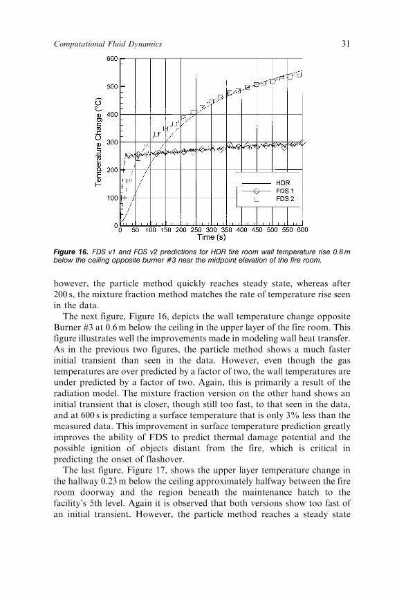
The next figure, Figure 16, depicts the wall temperature change oppositeBurner #3 at 0.6 m below the ceiling in the upper layer of the fire room. Thisfigure illustrates well the improvements made in modeling wall heat transfer.As in the previous two figures, the particle method shows a much fasterinitial transient than seen in the data. However, even though the gastemperatures are over predicted by a factor of two, the wall temperatures areunder predicted by a factor of two. Again, this is primarily a result of theradiation model. The mixture fraction version on the other hand shows aninitial transient that is closer, though still too fast, to that seen in the data,and at 600 s is predicting a surface temperature that is only 3% less than themeasured data. This improvement in surface temperature prediction greatlyimproves the ability of FDS to predict thermal damage potential and thepossible ignition of objects distant from the fire, which is critical inpredicting the onset of flashover.

The last figure, Figure 17, shows the upper layer temperature change inthe hallway 0.23 m below the ceiling approximately halfway between the fireroom doorway and the region beneath the maintenance hatch to thefacility’s 5th level. Again it is observed that both versions show too fast ofan initial transient. However, the particle method reaches a steady state

Figure 16. FDS v1 and FDS v2 predictions for HDR fire room wall temperature rise 0.6 mbelow the ceiling opposite burner #3 near the midpoint elevation of the fire room.


temperature change approximately 15% lower than the mixture fractionversion. This is surprising since the initial temperature change of the upperlayer in the fire room was a factor of two higher. This would suggest thatthe heat transfer to the hallway ceiling is being greatly over predicted by theparticle method. The mixture fraction version, which over predictsthe hallway temperature rise by 12%, is slightly under predicting the heattransfer to the ceiling, a result which is similar to that seen in the fire roomwall temperature. Since radiation heat transfer plays a much smaller role inthe hallway due to the lower temperatures, the improvements seen in thislocation are likely the result of modifications to the convective heat transfermodel in FDS [1].

The final HDR comparisons are for a set of gas sensors located in thecenterline of the doorway, 0.16 m below the doorway soffit. Four sensorswere placed here, CO2, CO, unburned hydrocarbons, and O2. Only the CO2

and O2 sensors generated useable data for this test. At 10min, the sensorsindicated respective concentrations of 8.0 and 11.5% whereas mixturefraction predictions were 7.2 and 7.7%. For this simulation, the mixturefraction is still predicting well the CO2 concentration at this point, but isover predicting the oxygen consumption at this point. It is not clear why thisis the case, though it may result from the actual test using premixed air andfuel which cannot be directly simulated with the mixture fraction concept asimplemented.

Figure 17. FDS v1 and FDS v2 predictions for HDR hallway upper layer temperature rise0.23 m below the ceiling midway between fire room and hatch to 5th level.


CONCLUSIONS

A new combustion model and a new radiation model have been added toFDS v1 as part of a series of enhancements to create a new version of FDS,which has been released as v2. The new combustion model is a mixturefraction model modified to work on the coarse grids usually used insimulating compartment fires. This model adds the ability to track majorcombustion species with only a small added computational cost. Themixture fraction model may also be extended to include minor species onceappropriate data concerning state relationships for compartment fires canbe developed. The new radiation model allows FDS to model gas–gas andgas–surface radiation heat transfer, which was not possible in the originalmodel.

To test the new version of FDS and to compare it with the previousrelease, two sets of simulations were done. The first set was a simulation ofthree different pool fires. Since this set involved nonventilation controlledfires that do not form hot gas layers, the results are a good comparison ofpredictive changes caused solely by the combustion model. The second setinvolved two compartment fires including a 400 kW fire in the NIST 40%Reduced Scale Enclosure, which was ventilation controlled and a 1MW firein the HDR test facility, which was not ventilation controlled.

The plume tests clearly indicate two things. First, since both versionspredict nearly the same results in the far-field, it is clear that the changesmade to add the mixture fraction and finite volume radiation models, did notadversely affect the hydrodynamics solution. Second, the results illustratewell a major advantage of the mixture fraction model. Since the mixturefraction model preserves the single step chemical reaction and has the fuel asa gas rather than solid particles, the volume where combustion takes place ismore realistic. With the Lagrangian particle method, combustion occurs tooclose to burner surface and the burner’s centerline. This is not realistic,as that region in reality will contain little oxygen to support combustion.The mixture fraction model, however, has the combustion occurring near theedge of the burner. It still has numerical artifacts, which can be seen inthe region of intense combustion at the burner’s edge where the coarseness ofthe grid results in overly high mixture fraction gradients at that location.

The compartment fire simulations also show that the new version of FDSis an improvement over the particle method. Temperature predictions,especially the lower layer temperatures, are greatly improved with the newversion. This is mostly a result of the new radiation model. However, thereare also some minor benefits from the mixture fraction model which doesaccount for the small changes in total moles of gas that result fromcombusting a hydrocarbon, which has a slight impact on the mass flow


predictions, which in turn impacts the temperature predictions. The mixturefraction also managed to reasonably predict major species concentrationsexiting the compartment. This represents a major improvement over FDSv1, which did not have this capability.

The compartment simulations indicate that further improvements couldbe made to the mixture fraction model. The comparison of gas concentra-tions in the doorway, notably the complete lack of oxygen, and thecomparison of the FDS results with visual observations indicate that thecombusting surface in the mixture fraction model is too small. That is, toomuch combustion is taking place inside the compartment. An extension ofthe mixture fraction model to account for combustion inefficiencies duringunderventilated fires might improve the prediction of the flame surface,which in turn should lead to lower upper layer temperatures. The inclusionof a reaction progress parameter would also allow for a better simulation ofpremixed fuels.

In conclusion, the mixture fraction combustion model and finite volumemethod radiation solver were successfully implemented in FDS. Theseimprovements result in markedly improved predictive capabilities for thecases tested. However, these are not the only benefits. The mixture fraction,as a single species, through its state relationships, see Figure 1, containsinformation about combustion products. It is hoped that the currentidealized combustion can be expanded to more realistically include minorspecies such as soot and CO, e.g., by creating a two-parameter mixturefraction that includes a reaction progress variable as opposed to merelyspecifying a fixed CO/CO2 production ratio. The new radiation model,which includes gas-to-surface and surface-to-surface radiation heat transferenables FDS to begin making plausible predictions of object ignition timesfor flashover prediction. While further development could improve bothmodels, the mixture fraction combustion model and the finite volumeradiation transport model are a significant improvement over theLagrangian particle model and the ray-tracing model.

NOMENCLATURE

D�=Dt substantial or material derivative of �ijk cell indicesI radiation intensity (W/m2)Ib radiation source term (W/m2)_mm000

i production rate of change of species i per unit volume (kg/s m3)_mm00

i production rate of change of species i per unit area (kg/s m2)n normal vector


s oxygen mass to fuel mass ratio for stoichiometry (kg O2/kg fuel)ss path vectort time (s)T temperature (K)x position vector (m)V volume (m3)Z mixture fractionZF stoichiometric value of the mixture fractionYi mass fraction (kg species i/kg gas)wi molecular weight of species i (g/mol)�i yield of species i (moles species i/moles fuel burned)� absorptivity (1/m)�i stoichiometric coefficient of species i (moles)� density (kg/m3) Stefan–Boltzman constant (W/m2 K4)� ratio of supplied air to stoichiometrically required air (moles air

supplied/moles required)

REFERENCES

1. McGrattan, K. et al., Fire Dynamics Simulator (Version 2) – Technical Reference Guide,NISTIR 6783, National Institute of Standards and Technology, Gaithersburg, MD, 2001.

2. McGrattan, K. and Forney, G., Fire Dynamics Simulator (Version 2) – User’s Manual,NISTIR 6784, National Institute of Standards and Technology, Gaithersburg, MD, 2001.

3. Kuo, K., Principles of Combustion, New York, NY, John Wiley and Sons, 1986.

4. Raithby, G. and Chui, E., ‘‘A Finite-Volume Method for Predicting Radiant Heat Transferin Enclosures with Participating Media’’, Journal of Heat Transfer, Vol. 112, 1990, pp. 415–423.

5. Rehm, R. and Baum, H., ‘‘The Equations of Motion for Thermally Driven, BuoyantFlows’’, Journal of Research of the NBS, Vol. 83, 1978, pp. 297–308.

6. Mahalingam, S. et al., ‘‘Analysis and Numerical Simulation of a Nonpremixed Flame in aCorner’’, Combustion and Flame, Vol. 118, 1999, pp. 221–232.

7. Siegel, R. and Howell, J.R. Thermal Radiation Heat Transfer, 3rd Edn., Philadelphia, PA,Hemisphere Publishing Corp., 1992.

8. Karlsson, B. and Quintiere, J., Enclosure Fire Dynamics, Boca Raton, FL, CRC Press, 2000.

9. Mulholland, G. and Choi, M. Measurement of the Mass Specific Extinction Coefficient forAcetylene and Ethene Smoke Using the Large Agglomerate Optics Facility, 27thSymposium on Combustion, The Combustion Institute, 1998, pp. 1515–1522.

10. Grosshandler, W., RADCAL: A Narrow-Band Mode for Radiation Calculations in aCombustion Environment, NIST Technical Note 1402, National Institute of Standards andTechnology, Gaithersburg, MD, 1993.

11. Baum, H. et al., ‘‘Three Dimensional Simulations of Fire Plume Dynamics’’, In: Pro-ceedings of the 5th International IAFSS Symposium, Fire Safety Science, 1997, pp. 511–522.

12. Blevins, L., ‘‘Behavior of Bare and Aspirated Thermocouples in Compartment Fires,HTD99–280’’, In: Proceedings of the ASME National Heat Transfer Conference,Albuquerque, NM, 1999.


13. Schall, M. and Valencia, L., Data Compilation of the HDR Containment for Input DataProcessing for Pre-Test Calculations, PHDR Working Report 3.143/79, Project HDRNuclear Center, Karlsruhe, Germany, 1982.

14. Floyd, J., Evaluation of the Predictive Capabilities of Current Computational Methods forFire Simulation in Enclosures Using the HDR T51 and T52 Tests with a Focus onPerformance-Based Fire Codes, Ph.D. Dissertation, University of Maryland, College Park,MD, 2000.

15. Floyd, J., Comparison of CFAST and FDS for Fire Simulation with the HDR T51 and T52Tests, NISTIR-6866, National Institute of Standards and Technology, Gaithersburg, MD,2002.


Documents

FLOYD All CFD Fire Simulations Using Mixture Fraction Combust Journal of Fire Protect Engineering 13-11-26 2003