1

Flow Measurement in Pipes and Ducts

Dr. Harlan H. Bengtson, P.E.

COURSE CONTENT

1. Introduction

This course is about measurement of the flow rate of a fluid flowing under

pressure in a closed conduit. The closed conduit is often circular, but also may be

square or rectangular (such as a heating duct) or any other shape. The other

major category of flow is open channel flow, which is the flow of a liquid with a

free surface open to atmospheric pressure. Measurement of the flow rate of a

fluid flowing under pressure, is carried out for a variety of purposes, such as

billing for water supply to homes or businesses or, for monitoring or process

control of a wide variety of industrial processes that involve flowing fluids.

Several categories of pipe flow measurement devices will be described and

discussed, including some associated calculations.

2

2. Learning Objectives

At the conclusion of this course, the student will

• Be able to calculate liquid flow rate from measured pressure difference,

fluid properties, and meter parameters, using the provided equations for

venturi, orifice, and flow nozzle meters.

• Be able to calculate gas flow rate from measured pressure difference, fluid

properties, and meter parameters, using the provided equations for venturi,

orifice, and flow nozzle meters.

• Be able to determine which type of ISO standard pressure tap locations are

being used for a given orifice meter.

• Be able to calculate the orifice coefficient, Co, for specified orifice and pipe

diameters, pressure tap locations and fluid properties.

• Be able to estimate the density of a specified gas at specified temperature

and pressure using the Ideal Gas Equation.

• Be able to calculate the velocity of a fluid for given pitot tube reading and

fluid density.

• Know the general configuration and principle of operation of rotameters

and positive displacement, electromagnetic, target, turbine, vortex,

ultrasonic, coriolis mass, and thermal mass meters.

• Know recommended applications for each of the type of flow meter

discussed in this course.

3

• Be familiar with the general characteristics of the types of flow meters

discussed in this course, as summarized in Table 2 near the end of this

document.

3. Types of Pipe Flow Measurement Devices

The types of pipe flow measuring devices to be discussed in this course are as

follows:

i) Differential pressure flow meters

a) Venturi meter

b) Orifice meter

c) Flow nozzle meter

ii) Velocity flow meters – pitot / pitot-static tubes

iii) Variable area flow meters - rotameters

iv) Positive displacement flow meters

v) Miscellaneous

a) Electromagnetic flow meters

b) Target flow meters

d) Turbine flow meters

e) Vortex flow meters

4

f) Ultrasonic flow meters

g) Coriolis mass flow meters

h) Thermal mass flow meters

4. Differential Pressure Flow meters

Three types of commonly used differential pressure flow meters are the orifice

meter, the venturi meter, and the flow nozzle meter. These three all function

by introducing a reduced area through which the fluid must flow. The decrease in

area causes an increase in velocity, which in turn results in a decrease in pressure.

With these flow meters, the pressure difference between the point of maximum

velocity (minimum pressure) and the undisturbed upstream flow is measured and

can be correlated with flow rate.

Using the principles of conservation of mass (the continuity equation) and the

conservation of energy (the energy equation without friction or Bernoulli

equation), the following equation can be derived for ideal flow between the

upstream, undisturbed flow (subscript 1) and the downstream conditions where

the flow area is constricted (subscript 2):

Where: Qideal = ideal flow rate (neglecting viscosity and other friction

effects), cfs

A2 = constricted cross-sectional area normal to flow, ft2

5

P1 = upstream (undisturbed) pressure in pipe, lb/ft2

P2 = pressure in pipe where flow area is constricted to A2, lb/ft2

= D2/D1 = (diam. at A2)/(pipe diam.)

= fluid density, slugs/ft3

A discharge coefficient, C, is typically put into equation (1) to account for friction

and any other non-ideal factors, giving the following general equation for

differential pressure meters:

Where: Q = flow rate through the pipe and meter, cfs

C = discharge coefficient, dimensionless

All other parameters are as defined above

Measurement of Gas Flows: Equations (1) and (2) apply for either liquid flow

or gas flow through differential pressure flow meters. For measurement of liquid

flow, the density can typically be assumed to be constant throughout the meter,

however, for measurement of gas flow, with a reasonable pressure change across

the meter, the density will change enough so that it can’t be taken as constant in

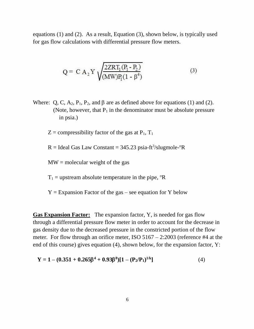
6

equations (1) and (2). As a result, Equation (3), shown below, is typically used

for gas flow calculations with differential pressure flow meters.

Where: Q, C, A2, P1, P2, and are as defined above for equations (1) and (2).

(Note, however, that P1 in the denominator must be absolute pressure

in psia.)

Z = compressibility factor of the gas at P1, T1

R = Ideal Gas Law Constant = 345.23 psia-ft3/slugmole-oR

MW = molecular weight of the gas

T1 = upstream absolute temperature in the pipe, oR

Y = Expansion Factor of the gas – see equation for Y below

Gas Expansion Factor: The expansion factor, Y, is needed for gas flow

through a differential pressure flow meter in order to account for the decrease in

gas density due to the decreased pressure in the constricted portion of the flow

meter. For flow through an orifice meter, ISO 5167 – 2:2003 (reference #4 at the

end of this course) gives equation (4), shown below, for the expansion factor, Y:

Y = 1 – (0.351 + 0.2654 + 0.938)[1 – (P2/P1)1/k] (4)

7

(for P2/P1 > 0.75)

Where , P1 and P2 are the diameter ratio, inlet pressure and pressure at

constriction, as defined above, and k is the specific heat ratio (Cp/Cv) for the gas.

For flow through a venturi meter, ISO 5167 – 4:2003 (reference #5 at the end of

this course) gives equation (5), shown below, for the expansion factor, Y. This

expression for Y is often used for flow nozzle meter calculations also.

Where and k are the diameter ratio and specific heat ratio as defined above, and

is the pressure ratio, P2/P1.

Each of the three types of differential pressure flow meters will now be

considered separately.

Venturi Meter: Fluid enters a venturi meter through a converging cone of angle

15o to 20o. It then passes through the throat, which has the minimum cross-

sectional area, maximum velocity, and minimum pressure in the meter. The fluid

then slows down through a diverging cone of angle 5o to 7o, for the transition

back to the full pipe diameter. Figure 1 shows the shape of a typical venturi

meter and the parameters defined above as applied to this type of meter. D2 is the

8

diameter of the throat and P2 is the pressure at the throat. D1 and P1 are in the

pipe before entering the converging portion of the meter.

Figure 1. Venturi Meter Parameters

Due to the smooth transition to the throat and gradual transition back to full pipe

diameter, the head loss through a venturi meter is quite low and the discharge

coefficient is quite high. For a venturi meter the discharge coefficient is typically

called the venturi coefficient, Cv, giving the following equation for liquid flow

through a venturi meter:

The value of the venturi coefficient, Cv, will typically range from 0.95 to nearly

one. In ISO 5167 ( ISO 5167-4:2003 – see reference #5 for this course), Cv is given

9

as 0.995 for cast iron or machined venturi meters and 0.985 for welded sheet

metal venturi meters meeting ISO specifications, all for Reynold’s Number

between 2 x 105 and 106. Information on the venturi coefficient will typically be

provided by venturi meter manufacturers or vendors.

Example #1: Water at 50o F is flowing through a venturi meter with a 2 inch

throat diameter, in a 4 inch diameter pipe. Per manufacturer’s information, Cv =

0.984 for this meter under these flow conditions. What is the flow rate through

the meter if the pressure difference, P1 – P2, is measured as 8 inches of Hg?

Solution: The density of water in the temperature range from 32o to 70oF is 1.94

slugs/ft3, to three significant figures, so that value will be used here. A2 =

D22/4 = ft2. = 2/4 = 0.5. Converting the pressure

difference to lb/ft2: P1 – P2 = (8 in Hg)(70.73 lb/ft2/in Hg) = 565.8 lb/ft2.

Substituting all of these values into equation (6):

There is a bit more to the calculation for flow of a gas through a venturi meter, as

illustrated with Example #2, which considers the flow of air through the same

meter used for water flow calculation in Example #1, with the same measured

pressure difference.

10

Example #2: Air at 50o F is flowing through a venturi meter with a 2 inch throat

diameter, in a 4 inch diameter pipe. Per manufacturer’s information, Cv = 0.984

for this meter under these flow conditions. What is the flow rate through the

meter if the pressure difference, P1 – P2, is measured as 8 inches of Hg and the

pressure in the pipe upstream of the meter is 20 psia?

Solution: As in Example #1: A2 = D22/4 = ft2. = 2/4

= 0.5, and the pressure difference of 8 in Hg is equal to 565.8 lb/ft2 for P1 – P2.

In order to use Equation (3) to calculate the flow rate of air through the venturi

meter, values are needed for the following parameters in addition to the values

identified above for A2, , and P1 – P2, the given value of 20 psia for P1 and the

value given above for the ideal gas law constant, R (345.23 psia-ft3/slugmole-oR).

• the compressibility factor of the air, Z

• the molecular weight of the air, MW

• the approach temperature of the air in oR, T1

• the expansion factor, Y

For a temperature of 50oF and pressure of 20 psia, the compressibility factor for

air can be taken to be one. The molecular weight of air is often rounded off to 29.

The absolute temperature T1 = 50 + 460 oR = 510 oR.

In order to use Equation (5) to calculate the expansion factor, Y, the parameter

can be calculated as:

= P2/P1 = P1 – (P2 – P1)/P1 = [(20*144) – 565.8]/(20*144) = 0.8035.

Using k = 1.4 for air and substituting values for k, , and into Equation (5) gives

Y = 0.881. Now, substituting all of the calculated parameter values into Equation

(3) gives:

11

This type of calculation can be facilitated by the use of an Excel spreadsheet set

up to make the calculations. An example with the solution to Example #2 is

shown below.

12

Orifice Meter: The orifice meter is the simplest of the three differential pressure

flow meters. It consists of a circular plate with a hole in the middle, typically

held in place between pipe flanges, as shown in figure 2.

Figure 2. Orifice Meter Parameters

For an orifice meter, the diameter of the orifice, d, will be used for D2, A2 is

typically called Ao, and the discharge coefficient is typically called an orifice

coefficient, Co, giving the following equation for liquid flow through an orifice

meter:

13

The preferred locations of the pressure taps for an orifice meter have undergone

change over time. Previously the downstream pressure tap was preferentially

located at the vena-contracta, the minimum jet area, which occurs downstream of

the orifice plate, as shown in Figure 2. For a vena-contracta tap, the tap location

depends on the orifice hole size. This link between the tap location and the

orifice size made it difficult to change orifice plates with different hole sizes in a

given meter in order to alter the range of measurement. In 1991, the ISO-5167

international standard came out, in which three types of standardized differential

measuring pressure taps were identified for orifice meters, as illustrated in Figure

3 below. In ISO-5167, the distance of the pressure taps from the orifice plate is

specified as a fixed distance or as a function of the pipe diameter, rather than the

orifice diameter as shown in Figure 3.

In ISO-5167, an equation for the orifice coefficient, Co, is given as a function of

, Reynolds Number, and L1 & L2, the distances of the pressure taps from the

orifice plate, as shown in Figures 2 and 3. This equation, given in the next

paragraph can be used for an orifice meter with any of the three standard pressure

tap configurations.

Figure 3. ISO standard orifice meter pressure tap locations

14

The ISO-5167 equation for Co is shown below as Equation (8): (The earlier

2001 version of this equation is given in reference #5 for this course, U.S. Dept.

of the Interior, Bureau of Reclamation, Water Measurement Manual).

Co = 0.5961 + 0.02612 + 0.000521 (106/Re)0.7

+ (0.0188 + 0.0063A)3.5(106/Re)0.3

+ (0.043 + 0.080e-10L1/D1 - 0.123 e-7L1/D1)(1 - 0.11A)[4/(1 - 4)]

- 0.031(M’2 = 0.8M’21.1)1.3 (8)

A = (19,000/Re)0.8 M’2 = 2(L2/D1)/(1 - )

If D1 < 2.8 in, then add the following term to Co: 0.011(0.75 - )(2.8 - D1)

Where: Co = orifice coefficient, as defined in equation (7), dimensionless

L1 = pressure tap distance from upstream face of the plate, inches

L2 = pressure tap distance from downstream face of the plate, inches

D = pipe diameter, inches

= ratio of orifice diameter to pipe diameter = d/D, dimensionless

Re = Reynolds number = DV/ = DV/, dimensionless (D in ft)

V = average velocity of fluid in pipe = Q/(D2/4), ft/sec (D in ft)

= kinematic viscosity of the flowing fluid, ft2/sec

= density of the flowing fluid, slugs/ft3

= dynamic viscosity of the flowing fluid, lb-sec/ft2

15

As shown in Figure 3: L1 = L2 = 0 for corner taps; L1 = L2 = 1 inch for flange

taps; and L1 = D & L2 = D/2 for D – D/2 taps. Equation (8) is not intended for

use with any other arbitrary values for L1 and L2.

The ISO 5167 standard includes several conditions required for use of equation

(8) as follows.

• For all three pressure tap configurations:

- d > 0.5 in

- 2 in < D1 < 40 in

- 0.1 < < 0.75

• For corner taps or (D – D/2) taps:

- Re > 5000 for 0.1 < < 0.56

- Re > 16,000 2 for > 0.56

• For flange taps:

- Re > 5000

- Re > 170 2(25.4 D1) (D1 in inches)

Fluid properties ( or & ) are needed in order to use equation (8). Tables or

graphs with values of , , and for water and other fluids over a range of

temperatures are available in many handbooks and fluid mechanics or

thermodynamics textbooks, as for example, in reference #1 for this course.

Table 1 shows density and viscosity for water at temperatures from 32o F to 70o F.

16

Table 1. Density and Viscosity of Water

Example #3: What is the Reynolds number for water at 50oF, flowing at 0.35 cfs

through a 4 inch diameter pipe?

Solution: Calculate V from V = Q/A = Q/(D2/4) = 0.35/[(4/12)2/4] = 4.01 ft/s.

From Table 1: = 1.407 x 10-5 ft2/s. From the problem statement: D = 4/12 ft.

Substituting into the expression for Re: Re = (4/12)(4.01)/(1.407 x 10-5)

Re = 9.50 x 104

17

Example #4: Use equation (8) to calculate Co for orifice diameters of 0.8, 1.6,

2.0, 2.4, & 2.8 inches, each in a 4 inch diameter pipe, with Re = 105, for each of

the standard pressure tap configurations: i) D – D/2 taps, ii) flange taps, and

iii) corner taps.

Solution: Making all of these calculations by hand using equation (8) would be

rather tedious, but once the equation is set up in an Excel spreadsheet, the

repetitive calculations are easily done. Following is a copy of the results from an

Excel spreadsheet solution to this problem.

18

Note that Co is between 0.597 and 0.617 for all three pressure tap configurations

for Re = 105 and between 0.2 and 0.7. For larger values of Reynolds number Co

will stay within this range. For smaller values of Reynolds number, Co will get

somewhat larger, especially for higher values of .

Example #5: Water at 50o F is flowing through an orifice meter with flange taps

and a 2 inch throat diameter, in a 4 inch diameter pipe. What is the flow rate

through the meter if the pressure difference, P1 – P2, is measured as 3.93 psi?

19

Solution: Assume Re is approximately 105, in order to get started. Then from

the solution to Example #4, with = 0.5: Co = 0.606.

From Table 1, the density of water at 50oF is 1.94 slugs/ft3 and its viscosity is

2.73 x 10-5 lb-sec/ft2. A2 = D22/4 = ft2. = 2/4 = 0.5.

Converting the pressure difference to lb/ft2: P1 – P2 = (8 in Hg)(70.73 lb/ft2/in

Hg) = 565.8 lb/ft2. Substituting all of these values into equation (7):

Check on Reynolds number value:

V = Q/A = 0.330/[ft/sec

Re = DV/ = (4/12)(3.78)/(1.407 x 10-5) = 8.9 x 104

This value is close enough to 105, so that the value used for Co is probably ok.

Alternate Solution to Example #5: The flow rate can be calculated directly

without using information from Example #4, by using an iterative calculation to

get the value for Co, as illustrated in the Excel spreadsheet screenshot shown on

the next page. Note that instructions are included for using Excel's Goal Seek

tool to carry out the iterative calculation of Co. Note that the value calculated for

Co here is also 0.606 to 3 significant digits and the value calculated for the flow

rate Q is 0.330 cfs, the same as that calculated above.

20

21

Note that the calculation is already pretty extensive to calculate the flow rate of a

liquid through an orifice meter, because of the complication of obtaining a value

for the orifice coefficient, Co. Additional steps are added for calculation of the

flow rate of a gas through an orifice meter, as illustrated in Example #2 for gas

flow through a venturi meter and in the next example for calculating the flow rate

of air through an orifice meter with the same pipe and orifice diameters and same

measured pressure difference as for water flow in Example #5.

Example #6: Air at 50o F is flowing through an orifice meter with flange taps

and a 2 inch throat diameter, in a 4 inch diameter pipe. What is the flow rate

through the meter if the pressure difference, P1 – P2, is measured as 3.93 psi and

the upstream pressure in the pipe, P1, is 20 psia?

Solution: The calculations will be similar to those used for Example #5, but

using Equation (3) for gas flow rather than Equation (7) for liquid flow through

an orifice meter. As in Example #5: A2 = D22/4 = ft2.

= 2/4 = 0.5, and the pressure difference, P1 – P2, is 3.93 psi.

In order to use Equation (3) to calculate the flow rate of air through the venturi

meter, values are needed for the following parameters in addition to the values

identified above for A2, , and P1 – P2, the given value of 20 psia for P1 and the

value given above for the ideal gas law constant, R (345.23 psia-ft3/slugmole-oR).

• the compressibility factor of the air, Z

• the molecular weight of the air, MW

• the approach temperature of the air in oR, T1

• the expansion factor, Y

• the viscosity of air at 50oF (4 x 10-7 lb-sec/ft2)

For a temperature of 50oF and pressure of 20 psia, the compressibility factor for

air can be taken to be one. The molecular weight of air is often rounded off to 29.

The absolute temperature T1 = 50 + 460 oR = 510 oR.

22

In order to use Equation (4) to calculate the expansion factor, Y, the ratio, P2/P1,

can be calculated as:

P2/P1 = P1 – (P2 – P1)/P1 = [(20*144) – 565.8]/(20*144) = 0.8035

Using k = 1.4 for air and substituting values for k, P2/P1, and into Equation (4)

gives:

Y = 1 – (0.351 + 0.265(0.54) + 0.93(0.58))[1 – (0.8035)1/1.4] = 0.946

Now an iterative calculation like that used in Example #5 is needed to get values

for Co and Q. Again, use of an Excel spreadsheet is a convenient way to carry out

this calculation including the required iteration. The following figure is a

screenshot showing the Excel spreadsheet solution to Example #6, showing the

solution as: Q = 7.55 cfs.

23

24

Flow Nozzle Meter: The flow nozzle meter is simpler and less expensive than a

venturi meter, but not quite as simple as an orifice meter. It consists of a

relatively short nozzle, typically held in place between pipe flanges, as shown in

Figure 4.

Figure 4. Flow Nozzle Meter Parameters

For a flow nozzle meter, the exit diameter of the nozzle, d, is used for D2 (giving

A2 = An), and the discharge coefficient is typically called a nozzle coefficient, Cn,

giving the following equation for a flow nozzle meter:

Due to the smoother contraction of the flow, flow nozzle coefficients are

significantly higher than orifice coefficients. They are not, however as high as

venturi coefficients. Flow nozzle coefficients are typically in the range from 0.94

to 0.99. There are several different standard flow nozzle designs. Information on

25

pressure tap placement and calibration should be provided by the meter

manufacturer.

5. Velocity Flow Meters – Pitot / Pitot-Static Tubes

Pitot tubes (also called pitot-static tubes) are an inexpensive, convenient way to

measure velocity at a point in a fluid. They are used widely in airflow

measurements in ventilation and HVAC applications. Definitions for three types

of pressure and how to measure those three different kinds of pressure are given

below, because understanding them helps to understand the pitot tube equation.

Static pressure, dynamic pressure and total pressure are defined below and

illustrated in figure 5.

Static pressure is the fluid pressure relative to surrounding atmospheric pressure,

measured through a flat opening, which is in parallel with the fluid flow, as

shown with the first U-tube manometer in Figure 5.

Stagnation pressure is the fluid pressure relative to the surrounding atmospheric

pressure, measured through a flat opening, which is perpendicular to and facing

into the direction of fluid flow, as shown with the second U-tube manometer in

Figure 5. This is also sometimes called the total pressure.

Dynamic pressure is the fluid pressure relative to the static pressure, measured

through a flat opening, which is perpendicular to and facing into the direction of

fluid flow, as shown with the third U-tube manometer in Figure 5. This is also

sometimes called the velocity pressure.

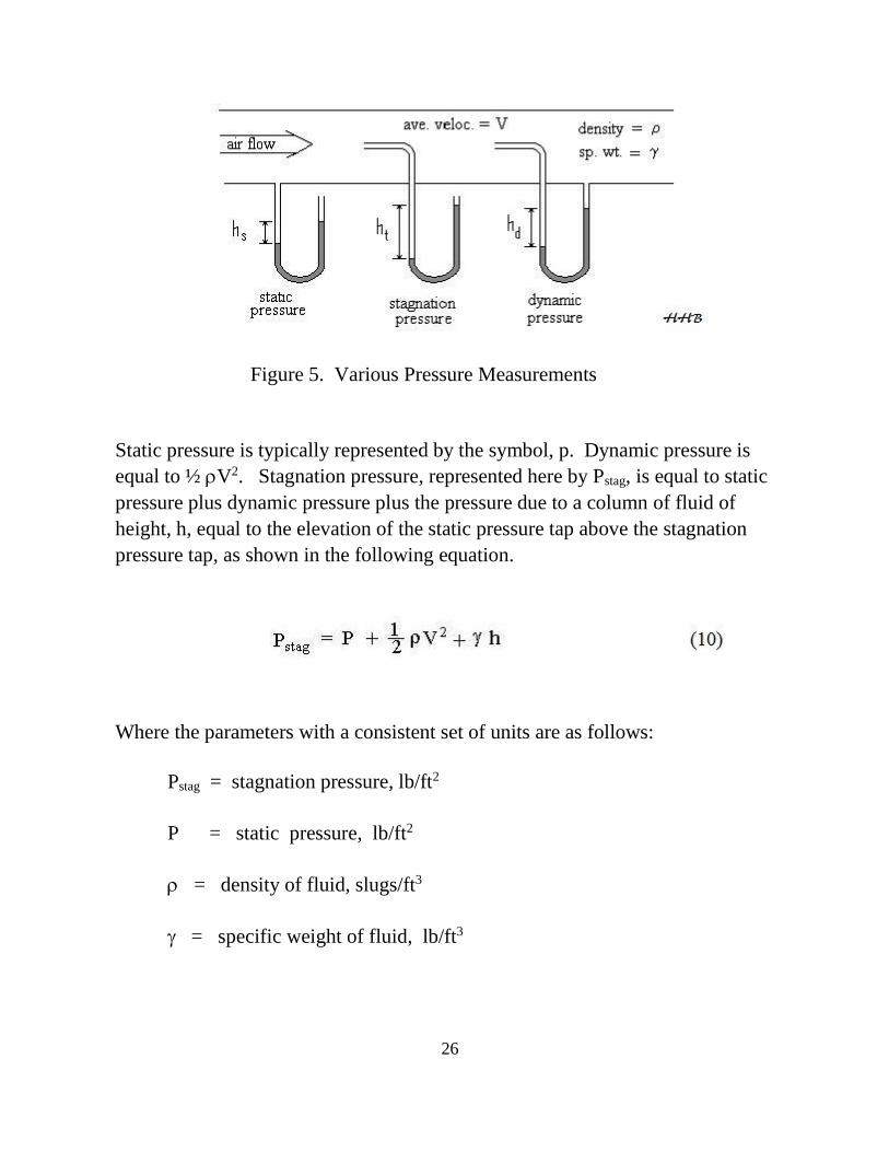
26

Figure 5. Various Pressure Measurements

Static pressure is typically represented by the symbol, p. Dynamic pressure is

equal to ½ V2. Stagnation pressure, represented here by Pstag, is equal to static

pressure plus dynamic pressure plus the pressure due to a column of fluid of

height, h, equal to the elevation of the static pressure tap above the stagnation

pressure tap, as shown in the following equation.

Where the parameters with a consistent set of units are as follows:

Pstag = stagnation pressure, lb/ft2

P = static pressure, lb/ft2

= density of fluid, slugs/ft3

= specific weight of fluid, lb/ft3

27

h = elevation of static pressure tap above stagnation pressure tap, ft

V = average velocity of fluid, ft/sec

(V = Q/A = volumetric flow rate/cross-sectional area normal to flow)

For pitot tube measurements, the static pressure tap and stagnation pressure tap

are at the same elevation, so that h =0. Then stagnation pressure minus static

pressure is equal to dynamic pressure, or:

The pressure difference, Pstag - P, can be measured directly with a pitot tube such

as the third U-tube in Figure 5, or more simply with a pitot tube like the one

shown in Figure 6, which has two concentric tubes. The inner tube has a

stagnation pressure opening and the outer tube has a static pressure opening

parallel to the fluid flow direction. The pressure difference is equal to the

dynamic pressure ( ½ V2 ) and can be used to calculate the fluid velocity for

known fluid density, . A consistent set of units is: pressure in lb/ft2, density in

slugs/ft3, and velocity in ft/sec.

28

Figure 6. Pitot Tube

For use with a pitot tube, equation (11) will typically be used to calculate the

velocity of the fluid. Setting (Pstag – P) = P, and solving for V, gives the

following equation:

In order to use Equation (12) to calculate fluid velocity from pitot tube

measurements, it is necessary to be able to obtain a value of density for the

flowing fluid at its temperature and pressure. For a liquid, a value for density can

typically be obtained from a table similar to Table 1 in this course. Such tables

are available in handbooks and fluid mechanics or thermodynamics textbooks.

Pitot tubes are used more commonly, however, to measure gas flow, as for

example, air flow in HVAC ducts, and density of a gas varies considerably with

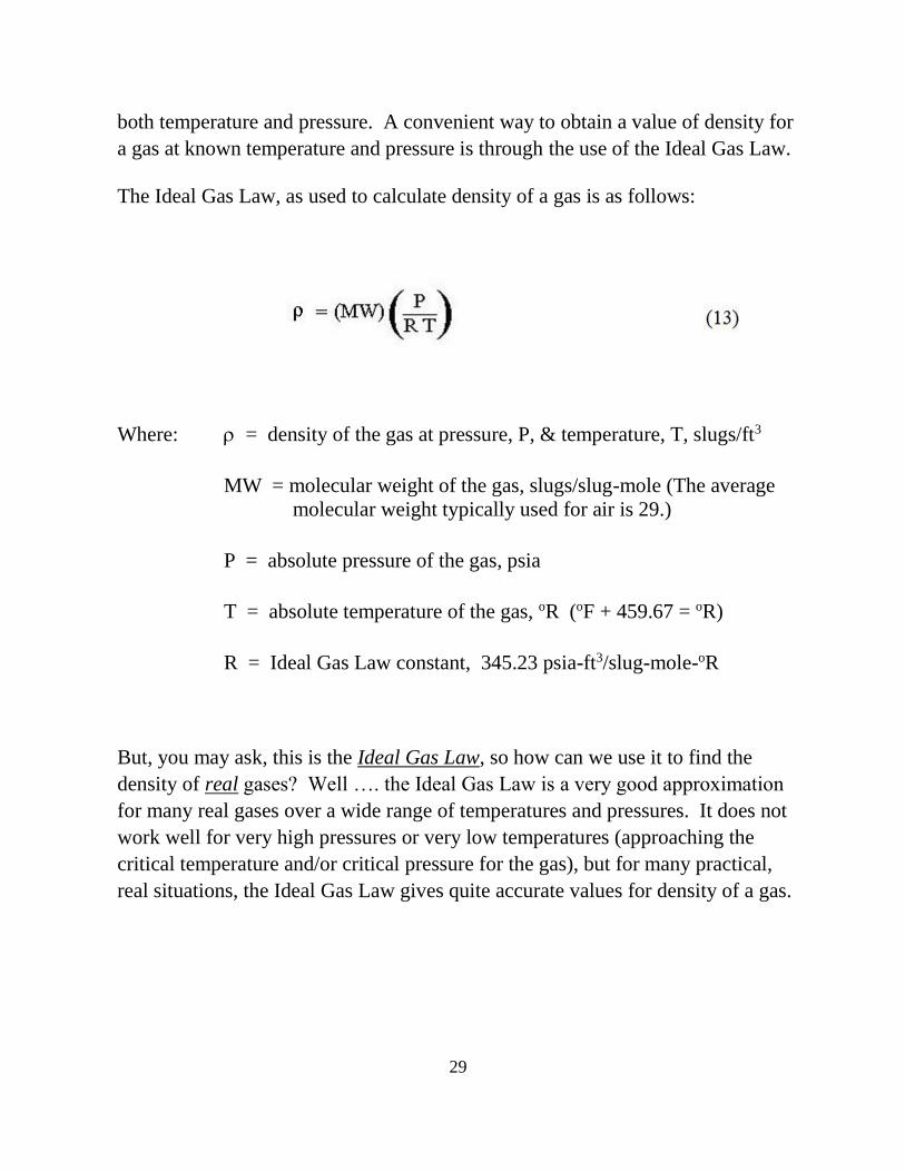
29

both temperature and pressure. A convenient way to obtain a value of density for

a gas at known temperature and pressure is through the use of the Ideal Gas Law.

The Ideal Gas Law, as used to calculate density of a gas is as follows:

Where: = density of the gas at pressure, P, & temperature, T, slugs/ft3

MW = molecular weight of the gas, slugs/slug-mole (The average

molecular weight typically used for air is 29.)

P = absolute pressure of the gas, psia

T = absolute temperature of the gas, oR (oF + 459.67 = oR)

R = Ideal Gas Law constant, 345.23 psia-ft3/slug-mole-oR

But, you may ask, this is the Ideal Gas Law, so how can we use it to find the

density of real gases? Well …. the Ideal Gas Law is a very good approximation

for many real gases over a wide range of temperatures and pressures. It does not

work well for very high pressures or very low temperatures (approaching the

critical temperature and/or critical pressure for the gas), but for many practical,

real situations, the Ideal Gas Law gives quite accurate values for density of a gas.

30

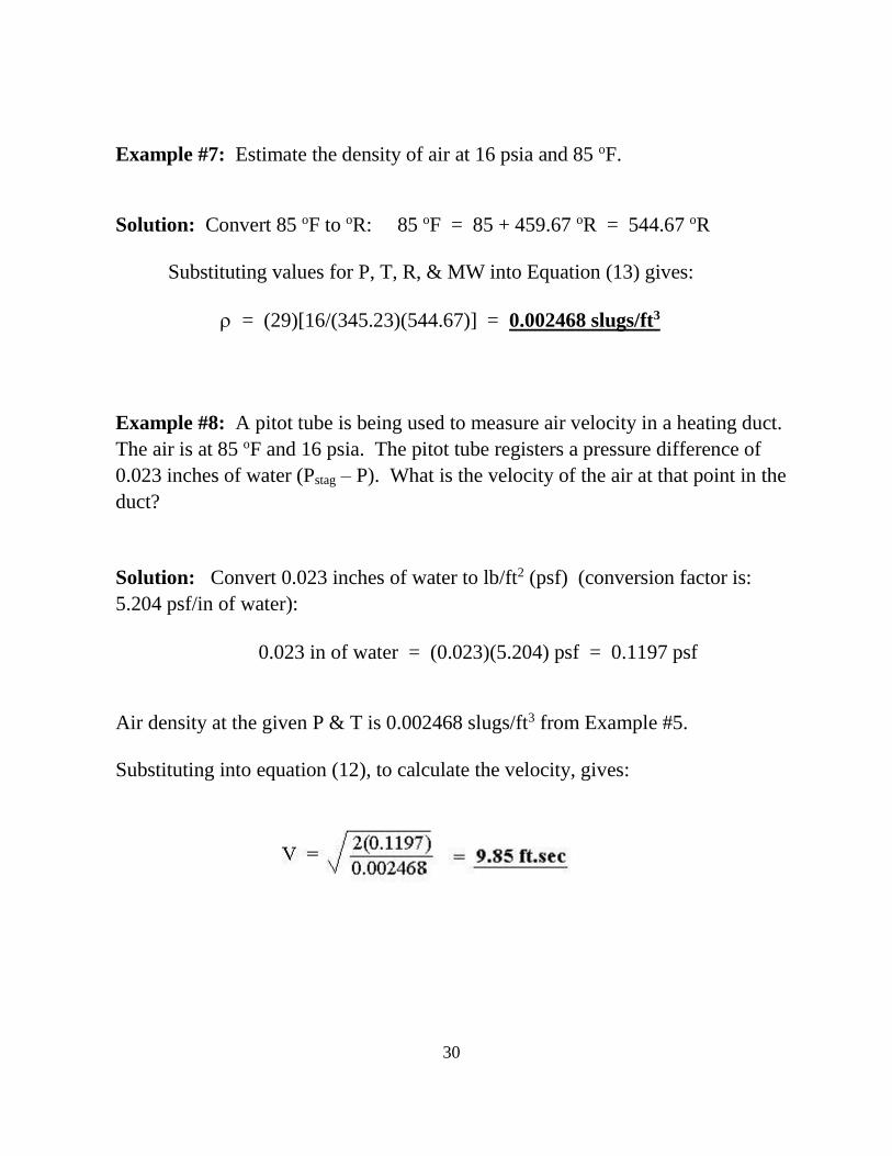
Example #7: Estimate the density of air at 16 psia and 85 oF.

Solution: Convert 85 oF to oR: 85 oF = 85 + 459.67 oR = 544.67 oR

Substituting values for P, T, R, & MW into Equation (13) gives:

= (29)[16/(345.23)(544.67)] = 0.002468 slugs/ft3

Example #8: A pitot tube is being used to measure air velocity in a heating duct.

The air is at 85 oF and 16 psia. The pitot tube registers a pressure difference of

0.023 inches of water (Pstag – P). What is the velocity of the air at that point in the

duct?

Solution: Convert 0.023 inches of water to lb/ft2 (psf) (conversion factor is:

5.204 psf/in of water):

0.023 in of water = (0.023)(5.204) psf = 0.1197 psf

Air density at the given P & T is 0.002468 slugs/ft3 from Example #5.

Substituting into equation (12), to calculate the velocity, gives:

31

6. Variable Area Flow Meter - Rotameters

A rotameter is a ‘variable area’ flow meter. It consists of a tapered glass or

plastic tube with a float that moves upward to an equilibrium position determined

by the flow rate of fluid going through the meter. For greater flow rate, a larger

cross-sectional area is needed for the flow, so the float is moved upward until the

upward force on it by the fluid is equal to the force of gravity pulling it down.

Note that the ‘float’ must have a density greater than the fluid, or it would simply

float to the top of the fluid. Given below, in figure 7, is a schematic diagram of a

rotameter, showing the principle of its operation.

The height of the float as measured by a graduated scale on the side of the

rotameter can be calibrated for flow rate of the fluid being measured in

appropriate flow units. A few points regarding rotameters follow:

➢ Because of the key role of gravity, rotameters must be installed vertically

➢ Typical turndown ratio is 10:1, that is flow rates as low as 1/10 of the

maximum reading can be accurately measured.

➢ Accuracy as good as 1% of full scale reading can be expected.

➢ Rotameters do not require power, so they are safer to use with flammable

fluids, than an instrument using power, which would need to be explosion

proof.

➢ A rotameter causes little pressure drop.

➢ It is difficult to apply machine reading and continuous recording with a

rotameter.

32

Figure 7. Rotameter Schematic diagram

7. Positive Displacement Flow Meters

Positive displacement flow meters are often used in residential and small

commercial applications. They are very accurate at low to moderate flow rates,

which are typical of these applications. There are several types of positive

displacement meters, such as reciprocating piston, nutating disk, oval gear, and

rotary vane. In all of them, the water passing through the meter, physically

displaces a known volume of fluid for each rotation of the moving measuring

element. The number of rotations is counted electronically or magnetically and

converted to the volume that has passed through the meter and/or flow rate.

Positive displacement meters can be used for any relatively nonabrasive fluid,

such as heating oils, Freon, printing ink, or polymer additives. The accuracy is

very good, approximately 0.1% of full flow rate with a turndown of 70:1 or more.

33

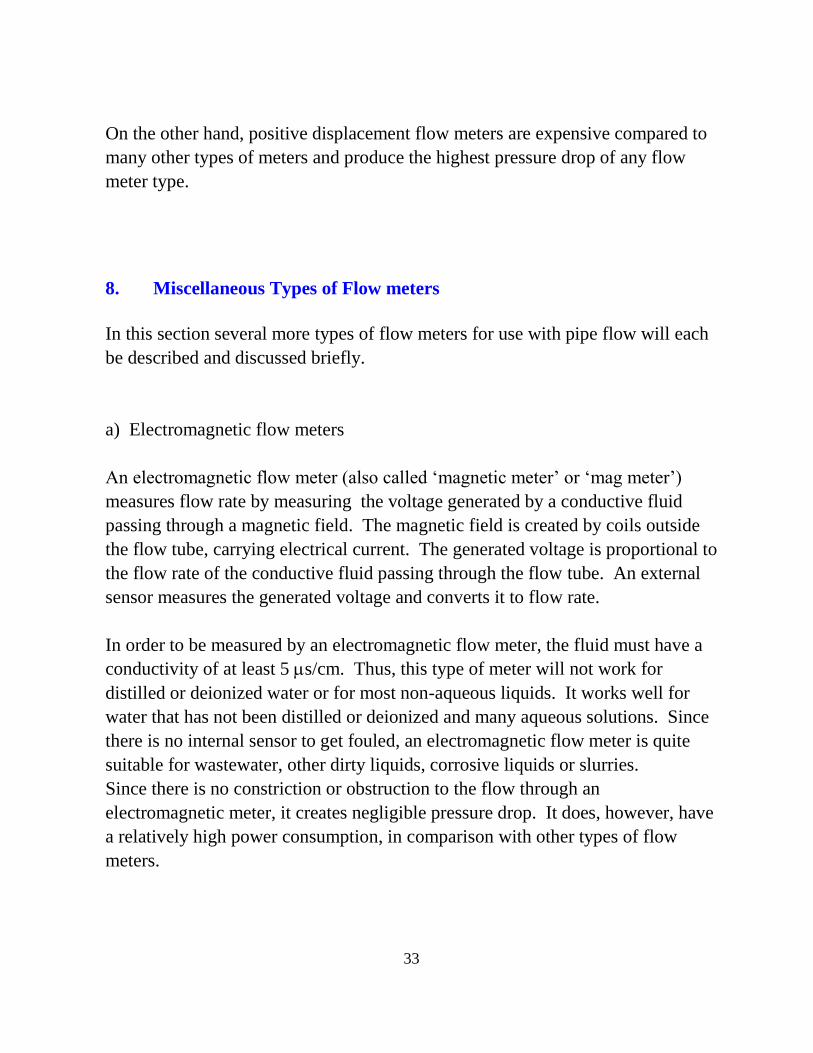
On the other hand, positive displacement flow meters are expensive compared to

many other types of meters and produce the highest pressure drop of any flow

meter type.

8. Miscellaneous Types of Flow meters

In this section several more types of flow meters for use with pipe flow will each

be described and discussed briefly.

a) Electromagnetic flow meters

An electromagnetic flow meter (also called ‘magnetic meter’ or ‘mag meter’)

measures flow rate by measuring the voltage generated by a conductive fluid

passing through a magnetic field. The magnetic field is created by coils outside

the flow tube, carrying electrical current. The generated voltage is proportional to

the flow rate of the conductive fluid passing through the flow tube. An external

sensor measures the generated voltage and converts it to flow rate.

In order to be measured by an electromagnetic flow meter, the fluid must have a

conductivity of at least 5 s/cm. Thus, this type of meter will not work for

distilled or deionized water or for most non-aqueous liquids. It works well for

water that has not been distilled or deionized and many aqueous solutions. Since

there is no internal sensor to get fouled, an electromagnetic flow meter is quite

suitable for wastewater, other dirty liquids, corrosive liquids or slurries.

Since there is no constriction or obstruction to the flow through an

electromagnetic meter, it creates negligible pressure drop. It does, however, have

a relatively high power consumption, in comparison with other types of flow

meters.

34

b) Target flow meters

With a target flow meter, a physical target (disk) is placed directly in the path of

the fluid flow. The target will be deflected due to the force of the fluid striking it,

and the greater the fluid flow rate, the greater the deflection will be. The

deflection is measured by a sensor mounted on the pipe and calibrated to flow

rate for a given fluid. Figure 8 shows a diagram of a target flow meter.

Figure 8. Target Flow Meter

A target flow meter can be used for a wide variety of liquids or gases and there

are no moving parts to wear out. They typically have a turndown of 10:1 to 15:1.

35

c) Turbine flow meters

A turbine flow meter operates on the principle that a fluid flowing past the blades

of a turbine will cause it to rotate. Increasing flow rate will cause increasing rate

of rotation for the turbine. The meter thus consists of a turbine placed in the path

of flow and means of measuring the rate of rotation of the turbine. The turbine’s

rotational rate can then be calibrated to flow rate. The turbine meter has one of

the higher turndown ratios, typically 20:1 or more. Its accuracy is also among the

highest at about + 0.25%.

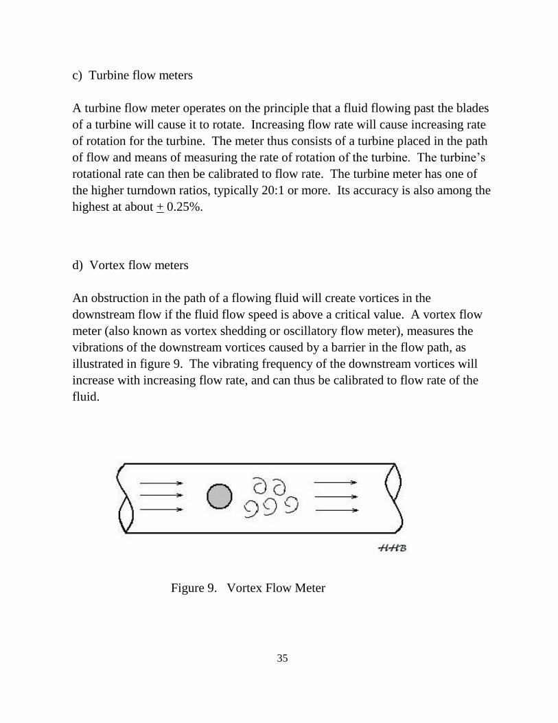
d) Vortex flow meters

An obstruction in the path of a flowing fluid will create vortices in the

downstream flow if the fluid flow speed is above a critical value. A vortex flow

meter (also known as vortex shedding or oscillatory flow meter), measures the

vibrations of the downstream vortices caused by a barrier in the flow path, as

illustrated in figure 9. The vibrating frequency of the downstream vortices will

increase with increasing flow rate, and can thus be calibrated to flow rate of the

fluid.

Figure 9. Vortex Flow Meter

36

e) Ultrasonic flow meters

The two major types of ultrasonic flow meters are ‘Doppler’ and ‘transit-time’

ultrasonic meters. Both use ultrasonic waves (frequency > 20 kHz). Both types

also use two transducers that transmit and/or receive the ultrasonic waves.

For the Doppler ultrasonic meter, one transducer transmits the ultrasonic waves

and the other receives the waves. The fluid must have material in it that will

reflect sonic waves, such as particles or entrained air. The frequency of the

transmitted beam of ultrasonic waves will be altered, by being reflected from the

particles or air bubbles. The resulting frequency shift is measured by the

receiving transducer, and is proportional to the flow rate through the meter. A

signal can thus be generated from the receiving transducer, which is proportional

to flow rate.

37

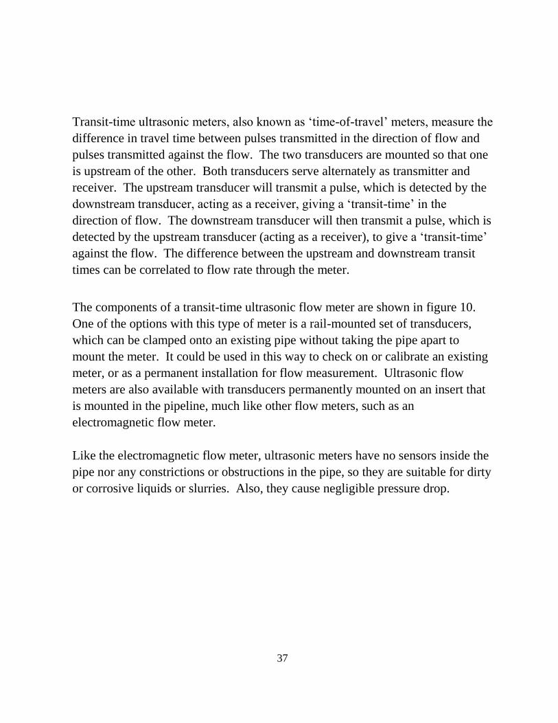
Transit-time ultrasonic meters, also known as ‘time-of-travel’ meters, measure the

difference in travel time between pulses transmitted in the direction of flow and

pulses transmitted against the flow. The two transducers are mounted so that one

is upstream of the other. Both transducers serve alternately as transmitter and

receiver. The upstream transducer will transmit a pulse, which is detected by the

downstream transducer, acting as a receiver, giving a ‘transit-time’ in the

direction of flow. The downstream transducer will then transmit a pulse, which is

detected by the upstream transducer (acting as a receiver), to give a ‘transit-time’

against the flow. The difference between the upstream and downstream transit

times can be correlated to flow rate through the meter.

The components of a transit-time ultrasonic flow meter are shown in figure 10.

One of the options with this type of meter is a rail-mounted set of transducers,

which can be clamped onto an existing pipe without taking the pipe apart to

mount the meter. It could be used in this way to check on or calibrate an existing

meter, or as a permanent installation for flow measurement. Ultrasonic flow

meters are also available with transducers permanently mounted on an insert that

is mounted in the pipeline, much like other flow meters, such as an

electromagnetic flow meter.

Like the electromagnetic flow meter, ultrasonic meters have no sensors inside the

pipe nor any constrictions or obstructions in the pipe, so they are suitable for dirty

or corrosive liquids or slurries. Also, they cause negligible pressure drop.

38

Figure 11. Transit-time Ultrasonic Flow Meter

f) Mass flow meters

The two types of mass flow meters will be described and discussed here. They

are the coriolis mass flow meter and thermal mass flow meter. Both of these

types of flow meters measure mass flow rate rather than volumetric flow rate.

Coriolis flow meters make use of the coriolis effect (a coriolis force that acts on

objects that are in motion relative to a rotating frame of reference. A coriolis

flow meter typically functions by generating a vibration of the tube or tubes that

the fluid is flowing through. Often the part of the tube that is vibrated is curved.

The amount of twist caused by the coriolis force is measured and is proportional

to the mass flow rate passing through the tube(s). Quite a variety of different

designs are used for coriolis mass flow meters.

Coriolis flow meters are among the most accurate of the types of flow meters

and have a very high turndown ratio (range from minimum to maximum readable

flow rate for a given meter.

39

A thermal mass flow meter typically includes a means of heat input to the

flowing fluid and for temperature measurement at two or more points. The

amount of temperature increase and rate of heat input to the fluid are measured

and can be correlated with the flow rate of the fluid through the thermal

properties of the fluid.

Thermal mass flow meters are among the most accurate of the types of flow

meters, have a very high turndown ratio (range from minimum to maximum

readable flow rate for a given meter) and have a medium cost. On the other hand,

they are only useable for the flow of clean gases and do not work well for gas

mixtures if the gas composition varies with time

9. Comparison of Flow Meter Alternatives

Table 2 shows a summary of several useful characteristics of the different types

of pipe flow meters described and discussed in this course. The information in

Table 2 was extracted from similar tables at the Omega Engineering and ICENTA

web sites at: http://www.omega.com/techref/table1.html and

http://www.icenta.co.uk/knowledge-base/flow-selection-guide/

The flow meter characteristics summarized in Table 2 are: recommended

applications, typical turndown ratio (also called rangeability), pressure drop,

typical accuracy, upstream pipe diameters (required upstream straight pipe

length), effect of viscosity, and relative cost.

40

41

10. Summary

There are a wide variety of meter types for measuring flow rate in closed

conduits. Fourteen of those types were described and discussed in this course.

This included a considerable amount of detail about pressure differential flow

meters (venturi, orifice and flow nozzle meters), such as equations and example

calculations for liquid flow and for gas flow through differential flow meters.

Table 2 in section 9, summarizes a comparison among those fourteen types of

42

flow meters. The fourteen types of flow meters discussed in this course and

compared in Table 2, are: Orifice meter, Venturi meter, Flow nozzle meter, Pitot

tube, Rotameter, Electromagnetic flow meter, Target meter, Turbine meter,

Vortex flow meter, Ultrasonic (Doppler) flow meter, Ultrasonic (time of travel)

flow meter, Coriolis mass flow meter, and Thermal mass flow meter. For each of

these types of flow meter, Table 2 provides information about i) recommended

applications, ii) typical turndown ratio, iii) whether its pressure drop is high,

medium, low, or none, iv) typical accuracy in %, v) required upstream pipe

diameters of straight pipe, vi) effect of viscosity, and vii) relative cost.

11. References

1. Bengtson, H.H., “Excel Spreadsheets for Orifice and Venturi Flow Meters,” an

online informational article at www.engineeringexcelspreadsheets.com

2. Bengtson, H.H., "Spreadsheets for ISO 5167 Orifice Plate Flow Meter

Calculations," an online informational article at

www.engineeringexcelspreadsheets.com

3. Munson, B. R., Young, D. F., & Okiishi, T. H., Fundamentals of Fluid

Mechanics, 4th Ed., New York: John Wiley and Sons, Inc, 2002.

4. International Organization of Standards - ISO 5167-2:2003 Measurement of

fluid flow by means of pressure differential devices inserted in circular cross-

section conduits flowing full, Part 2: Orifice plates. Reference number: ISO 5167-

2:2003.

43

5. International Organization of Standards - ISO 5167-4:2003 Measurement of

fluid flow by means of pressure differential devices inserted in circular cross-

section conduits flowing full, Part 4: Venturi Tubes. Reference number: ISO

5167-4:2003.

6. U.S. Dept. of the Interior, Bureau of Reclamation, 2001 revised, 1997 third

edition, Water Measurement Manual, available for on-line use or download at:

http://www.usbr.gov/pmts/hydraulics_lab/pubs/wmm/index.htm

7. LMNO Engineering, Research and Software, Ltd website. Contains equations

and graphs for flow measurement with venturi, orifice and flow nozzle

flowmeters. http://www.lmnoeng.com/venturi.htm

8. Engineering Toolbox website. Contains information on flow measurement

with a variety of meter types. http://www.engineeringtoolbox.com/fluid-flow-meters-

t_49.html