FAQ – Flow correlations © KAPPA 1988-2010 Emeraude - 1/12

Recommendations on flow correlations

This document aims at helping the Emeraude user in selecting a flow correlation when interpreting a Production Logging job. The following correlations are available in Emeraude:

Liquid-Gas Liquid-Liquid 3-Phase

Duns and Ross Nicolas 3-phase stratified Zhang

Aziz and Govier Choquette Stanford Drift Flux

Beggs and Brill ABB-Deviated

Artep Hasan & Kabir

Dukler Brauner

Hagedorn-Brown Stanford Drift Flux LL

Petalas & Aziz Constant slippage

Kaya et al.

Stanford Drift Flux LG

Constant slippage

You’ll find a short description of each correlation in the following sections, as well as some

recommendations on their usage.

FAQ – Flow correlations © KAPPA 1988-2010 Emeraude - 2/12

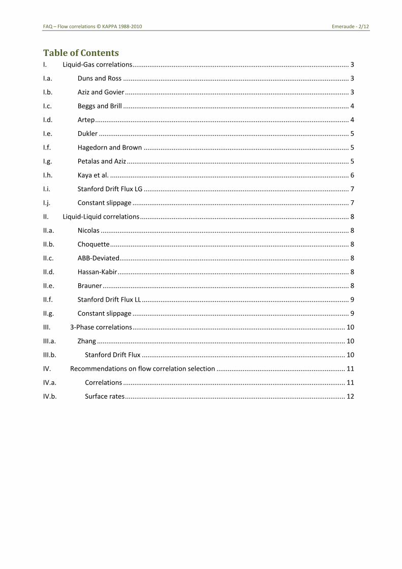
Table of Contents I. Liquid-Gas correlations .................................................................................................................... 3

I.a. Duns and Ross ......................................................................................................................... 3

I.b. Aziz and Govier ........................................................................................................................ 3

I.c. Beggs and Brill ......................................................................................................................... 4

I.d. Artep ........................................................................................................................................ 4

I.e. Dukler ...................................................................................................................................... 5

I.f. Hagedorn and Brown .............................................................................................................. 5

I.g. Petalas and Aziz ....................................................................................................................... 5

I.h. Kaya et al. ................................................................................................................................ 6

I.i. Stanford Drift Flux LG .............................................................................................................. 7

I.j. Constant slippage .................................................................................................................... 7

II. Liquid-Liquid correlations ................................................................................................................ 8

II.a. Nicolas ..................................................................................................................................... 8

II.b. Choquette ................................................................................................................................ 8

II.c. ABB-Deviated ........................................................................................................................... 8

II.d. Hassan-Kabir ............................................................................................................................ 8

II.e. Brauner .................................................................................................................................... 8

II.f. Stanford Drift Flux LL ............................................................................................................... 9

II.g. Constant slippage .................................................................................................................... 9

III. 3-Phase correlations .................................................................................................................. 10

III.a. Zhang ..................................................................................................................................... 10

III.b. Stanford Drift Flux ............................................................................................................. 10

IV. Recommendations on flow correlation selection ..................................................................... 11

IV.a. Correlations ....................................................................................................................... 11

IV.b. Surface rates ...................................................................................................................... 12

FAQ – Flow correlations © KAPPA 1988-2010 Emeraude - 3/12

I. Liquid-Gas correlations

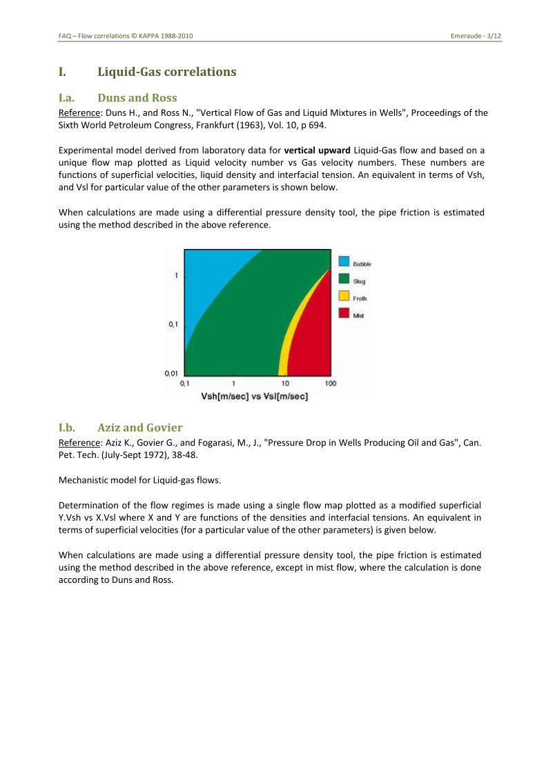
I.a. Duns and Ross Reference: Duns H., and Ross N., "Vertical Flow of Gas and Liquid Mixtures in Wells", Proceedings of the Sixth World Petroleum Congress, Frankfurt (1963), Vol. 10, p 694.

Experimental model derived from laboratory data for vertical upward Liquid-Gas flow and based on a unique flow map plotted as Liquid velocity number vs Gas velocity numbers. These numbers are functions of superficial velocities, liquid density and interfacial tension. An equivalent in terms of Vsh, and Vsl for particular value of the other parameters is shown below.

When calculations are made using a differential pressure density tool, the pipe friction is estimated using the method described in the above reference.

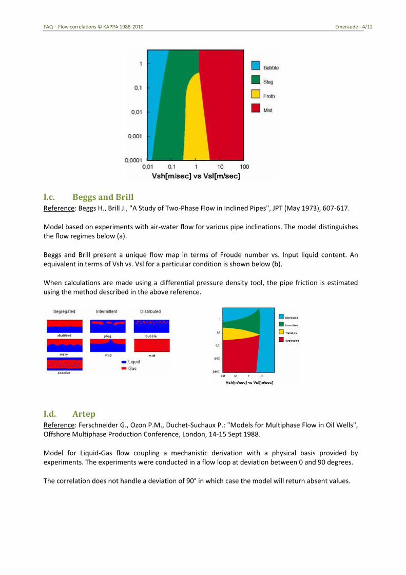
I.b. Aziz and Govier Reference: Aziz K., Govier G., and Fogarasi, M., J., "Pressure Drop in Wells Producing Oil and Gas", Can. Pet. Tech. (July-Sept 1972), 38-48.

Mechanistic model for Liquid-gas flows.

Determination of the flow regimes is made using a single flow map plotted as a modified superficial Y.Vsh vs X.Vsl where X and Y are functions of the densities and interfacial tensions. An equivalent in terms of superficial velocities (for a particular value of the other parameters) is given below.

When calculations are made using a differential pressure density tool, the pipe friction is estimated using the method described in the above reference, except in mist flow, where the calculation is done according to Duns and Ross.

FAQ – Flow correlations © KAPPA 1988-2010 Emeraude - 4/12

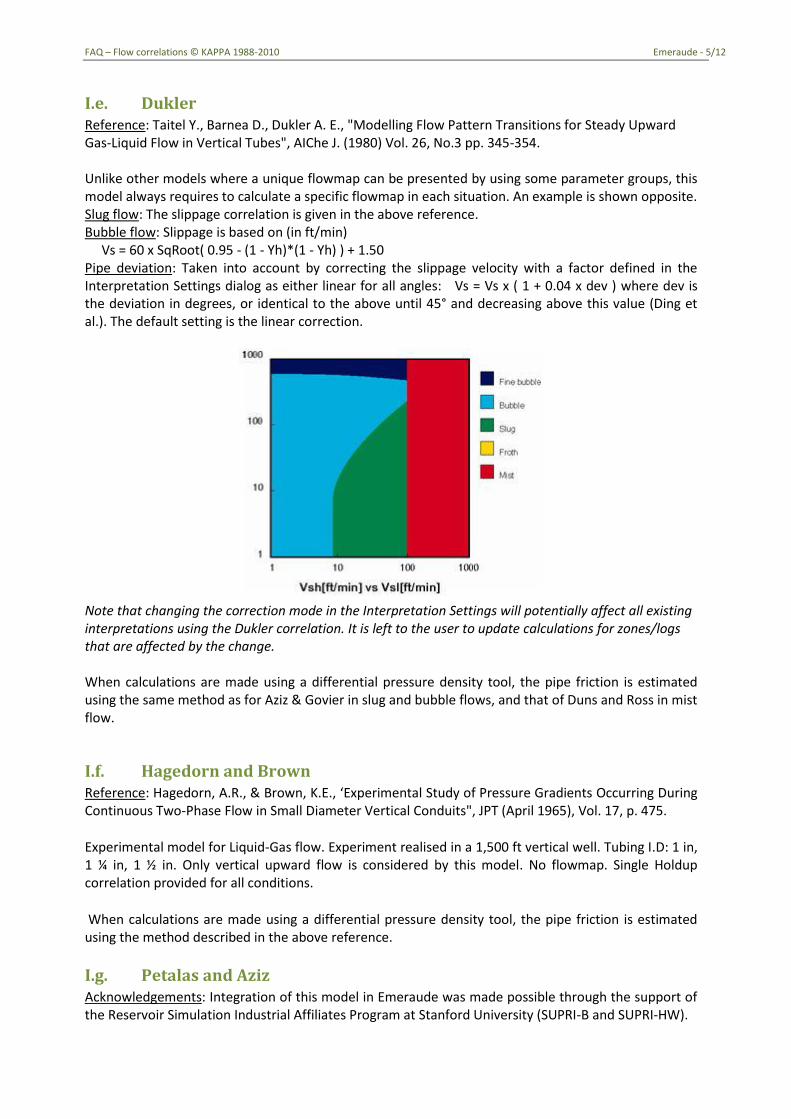
I.c. Beggs and Brill Reference: Beggs H., Brill J., "A Study of Two-Phase Flow in Inclined Pipes", JPT (May 1973), 607-617.

Model based on experiments with air-water flow for various pipe inclinations. The model distinguishes the flow regimes below (a).

Beggs and Brill present a unique flow map in terms of Froude number vs. Input liquid content. An equivalent in terms of Vsh vs. Vsl for a particular condition is shown below (b).

When calculations are made using a differential pressure density tool, the pipe friction is estimated using the method described in the above reference.

I.d. Artep Reference: Ferschneider G., Ozon P.M., Duchet-Suchaux P.: "Models for Multiphase Flow in Oil Wells", Offshore Multiphase Production Conference, London, 14-15 Sept 1988.

Model for Liquid-Gas flow coupling a mechanistic derivation with a physical basis provided by experiments. The experiments were conducted in a flow loop at deviation between 0 and 90 degrees.

The correlation does not handle a deviation of 90° in which case the model will return absent values.

FAQ – Flow correlations © KAPPA 1988-2010 Emeraude - 5/12

I.e. Dukler Reference: Taitel Y., Barnea D., Dukler A. E., "Modelling Flow Pattern Transitions for Steady Upward Gas-Liquid Flow in Vertical Tubes", AIChe J. (1980) Vol. 26, No.3 pp. 345-354. Unlike other models where a unique flowmap can be presented by using some parameter groups, this model always requires to calculate a specific flowmap in each situation. An example is shown opposite. Slug flow: The slippage correlation is given in the above reference. Bubble flow: Slippage is based on (in ft/min) Vs = 60 x SqRoot( 0.95 - (1 - Yh)*(1 - Yh) ) + 1.50 Pipe deviation: Taken into account by correcting the slippage velocity with a factor defined in the Interpretation Settings dialog as either linear for all angles: Vs = Vs x ( 1 + 0.04 x dev ) where dev is the deviation in degrees, or identical to the above until 45° and decreasing above this value (Ding et al.). The default setting is the linear correction.

Note that changing the correction mode in the Interpretation Settings will potentially affect all existing interpretations using the Dukler correlation. It is left to the user to update calculations for zones/logs that are affected by the change. When calculations are made using a differential pressure density tool, the pipe friction is estimated using the same method as for Aziz & Govier in slug and bubble flows, and that of Duns and Ross in mist flow.

I.f. Hagedorn and Brown Reference: Hagedorn, A.R., & Brown, K.E., ‘Experimental Study of Pressure Gradients Occurring During Continuous Two-Phase Flow in Small Diameter Vertical Conduits", JPT (April 1965), Vol. 17, p. 475.

Experimental model for Liquid-Gas flow. Experiment realised in a 1,500 ft vertical well. Tubing I.D: 1 in, 1 ¼ in, 1 ½ in. Only vertical upward flow is considered by this model. No flowmap. Single Holdup correlation provided for all conditions.

When calculations are made using a differential pressure density tool, the pipe friction is estimated using the method described in the above reference.

I.g. Petalas and Aziz Acknowledgements: Integration of this model in Emeraude was made possible through the support of the Reservoir Simulation Industrial Affiliates Program at Stanford University (SUPRI-B and SUPRI-HW).

FAQ – Flow correlations © KAPPA 1988-2010 Emeraude - 6/12

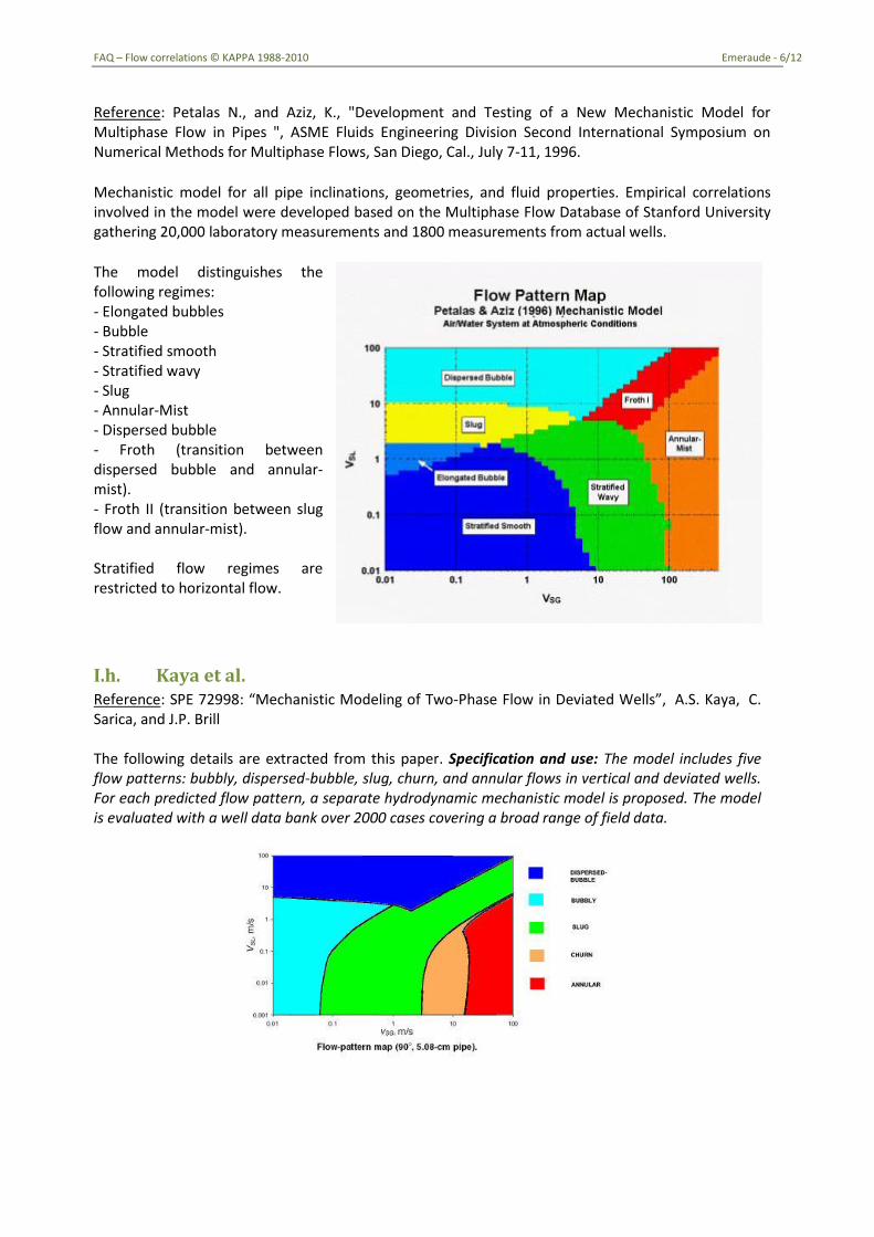
Reference: Petalas N., and Aziz, K., "Development and Testing of a New Mechanistic Model for Multiphase Flow in Pipes ", ASME Fluids Engineering Division Second International Symposium on Numerical Methods for Multiphase Flows, San Diego, Cal., July 7-11, 1996.

Mechanistic model for all pipe inclinations, geometries, and fluid properties. Empirical correlations involved in the model were developed based on the Multiphase Flow Database of Stanford University gathering 20,000 laboratory measurements and 1800 measurements from actual wells.

The model distinguishes the following regimes: - Elongated bubbles - Bubble - Stratified smooth - Stratified wavy - Slug - Annular-Mist - Dispersed bubble - Froth (transition between dispersed bubble and annular-mist). - Froth II (transition between slug flow and annular-mist). Stratified flow regimes are restricted to horizontal flow.

I.h. Kaya et al. Reference: SPE 72998: “Mechanistic Modeling of Two-Phase Flow in Deviated Wells”, A.S. Kaya, C. Sarica, and J.P. Brill The following details are extracted from this paper. Specification and use: The model includes five flow patterns: bubbly, dispersed-bubble, slug, churn, and annular flows in vertical and deviated wells. For each predicted flow pattern, a separate hydrodynamic mechanistic model is proposed. The model is evaluated with a well data bank over 2000 cases covering a broad range of field data.

FAQ – Flow correlations © KAPPA 1988-2010 Emeraude - 7/12

I.i. Stanford Drift Flux LG Reference: SPE 89836: “Drift-Flux Parameters for Three-Phase Steady-State Flow in Wellbores”; H. Shi, J.A. Holmes, L.R. Diaz, L.J. Durlofsky, K. Aziz The Drift-flux models represent multiphase flow in wellbores or pipes in terms of a number of empirically determined parameters. The great advantage of this model is that there is continuity between the various flow regimes. Two-phase model and parameter determination: The drift-flux model for two-phase gas-liquid flow is given by:

Vg = Co.Vm + Vd Where: Vg is the average gas in situ velocity,

Co is the profile parameter, Vm is the mixture velocity Vd is the drift velocity.

The parameters determining Co, Vm, and Vd are experimentally determined. Recommendations: Data used for the calibration were coming from cases with deviations from 0° to 88°. The model should not be used outside this range.

I.j. Constant slippage The slippage value is entered manually on each zone. When calculations are made using a differential pressure density tool, the pipe friction for all the above models is estimated using a Moody friction factor based for an Reynolds number representative of the mixture.

FAQ – Flow correlations © KAPPA 1988-2010 Emeraude - 8/12

II. Liquid-Liquid correlations

II.a. Nicolas Reference: Nicolas, Y., and Witterholt E.J.: "Measurements of Multiphase Fluid Flow", paper SPE 4023, 47th Annual SPE Fall Meeting, San Antonio, Texas, October 1972.

Experimental correlations for Liquid-Liquid bubble flow, relating the slippage velocity to the bubble rise velocity in a static column.

II.b. Choquette Reference: Choquette, Stanford University M.S. Thesis.

Experimental correlations for Liquid-Liquid bubble flow, relating the slippage velocity to the bubble rise velocity in a static column. This is a conventional slip velocity model in Water-Oil flow, represented as a chart giving the slippage versus the density difference for several values of water holdup.

II.c. ABB-Deviated Experimental correlations for Liquid-Liquid bubble flow, relating the slippage velocity to the bubble rise velocity in a static column. Variation of the Choquette correlation specifically derived from deviated wells data, recommended for Liquid-Liquid calculations in deviated wells.

II.d. Hassan-Kabir Reference: SPE 49163: "A Simplified Model for Oil-Water Flow in Vertical and Deviated Wellbores", A. R. Hasan, SPE, U. of North Dakota, and C. S. Kabir, SPE, Chevron Overseas Petroleum Technology Company. The study focuses on water-dominated flow regimes, close to bubbly flow, pseudo-slug flow, and chum flow. A drift-flux approach is taken to analyze the flow behavior of oil-water systems. Although simplistic, the proposed model appears to be quite robust in that it has reproduced a wide range of laboratory data from various sources. The model was validated versus different pipe sizes(1 to 8 in.), oil viscosity(1 to 150 cp) and production values(500 to 10,000 bpd).

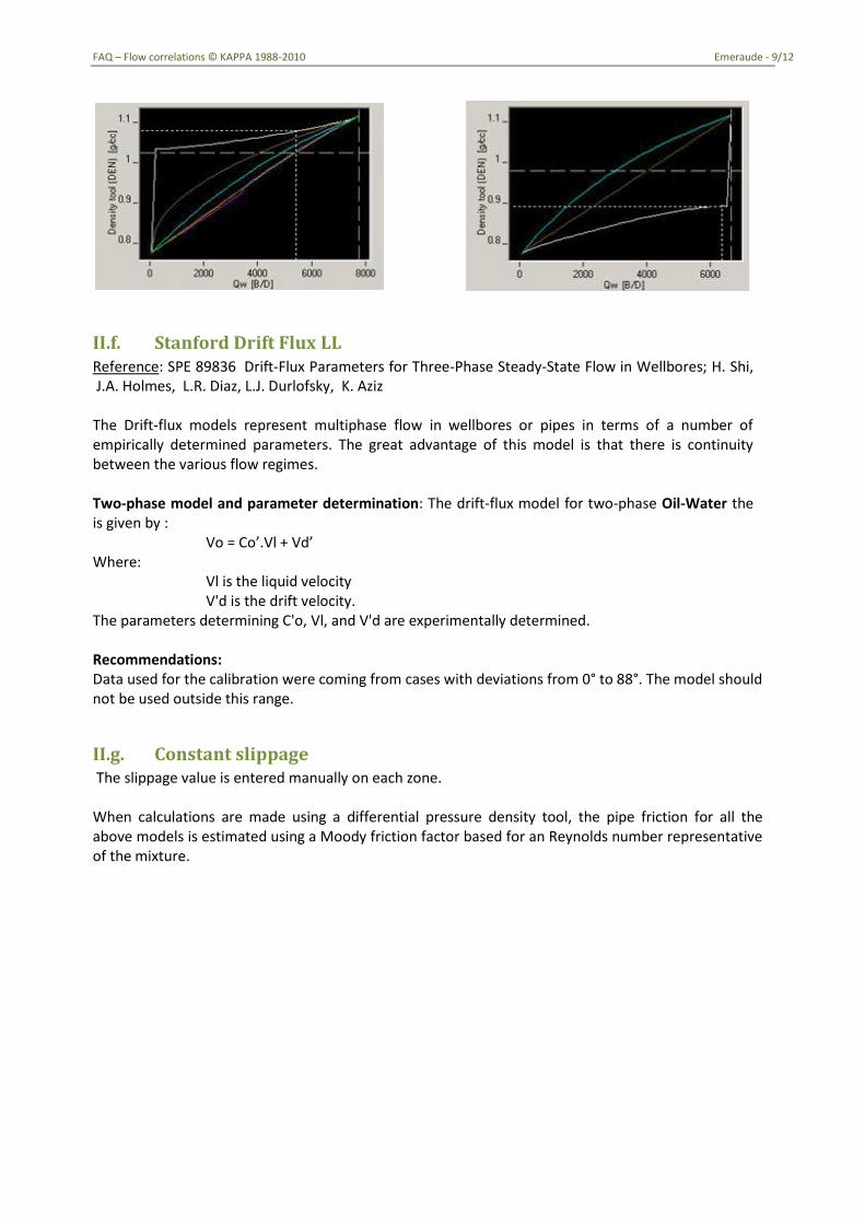
II.e. Brauner Reference: “Modeling and Control of Two-Phase Flow Phenomena" Neima Brauner Ed. V Bertola, CISM Center, Udine, Italy, 2004. Brauner is a combination of the Brauner stratified water-oil model, with the mechanistic model of Hasan & Kabir. The option is given to force stratified flow (in the Edit dialog). It is possible to force “on All” zones at once. Below are examples of the stratified flow predictions for upward and downward flows.

FAQ – Flow correlations © KAPPA 1988-2010 Emeraude - 9/12

II.f. Stanford Drift Flux LL Reference: SPE 89836 Drift-Flux Parameters for Three-Phase Steady-State Flow in Wellbores; H. Shi, J.A. Holmes, L.R. Diaz, L.J. Durlofsky, K. Aziz The Drift-flux models represent multiphase flow in wellbores or pipes in terms of a number of empirically determined parameters. The great advantage of this model is that there is continuity between the various flow regimes. Two-phase model and parameter determination: The drift-flux model for two-phase Oil-Water the is given by : Vo = Co’.Vl + Vd’ Where:

Vl is the liquid velocity V'd is the drift velocity.

The parameters determining C'o, Vl, and V'd are experimentally determined. Recommendations: Data used for the calibration were coming from cases with deviations from 0° to 88°. The model should not be used outside this range.

II.g. Constant slippage The slippage value is entered manually on each zone. When calculations are made using a differential pressure density tool, the pipe friction for all the above models is estimated using a Moody friction factor based for an Reynolds number representative of the mixture.

FAQ – Flow correlations © KAPPA 1988-2010 Emeraude - 10/12

III. 3-Phase correlations

III.a. Zhang Reference: SPE 95749, “Unified Modeling of Gas/Oil/Water pipe flow - Basic approach and preliminary validation.” H.-Q. Zhang, SPE and C.Sarica SPE, U. of Tulsa A three phase stratified flow model is extracted from this paper. It represents an evolution from the previous model presented by Zhang in ASME J.Energy Res. Tech. where the liquid phase was a fully mixed Oil + Water. This model should be used only in the case of proven stratified flow, since it does not include predictions for any other regime. In fact, when it is used outside its applicable range this model may exhibit a rather chaotic response (visible in the Zone Rates Plot). Furthermore, the model can only be applied in 3-phase. When one phase is absent, Emeraude internally switches to another model, with the logic: - Gas missing => Brauner; - Oil or Water missing => Petalas and Aziz.

III.b. Stanford Drift Flux Reference: SPE 89836 Drift-Flux Parameters for Three-Phase Steady-State Flow in Wellbores; H. Shi, J.A. Holmes, L.R. Diaz, L.J. Durlofsky, K. Aziz The Drift-flux models represent multiphase flow in wellbores or pipes in terms of a number of empirically determined parameters. The great advantage of this model is that there is continuity between the various flow regimes. Three-phase parameter determination To model three-phase flow, a two-stage approach is first applied based purely on the two-phase flow models. The system is first treated as a gas-liquid flow to determine the gas hold up and then model the liquid as an oil-water system to determine the liquid hold ups. Recommendations: Data used for the calibration were coming from cases with deviations from 0° to 88°. The model should not be used outside this range.

FAQ – Flow correlations © KAPPA 1988-2010 Emeraude - 11/12

IV. Recommendations on flow correlation selection

The choice of a particular correlation is especially critical in Liquid-Gas situations where the spread between the various models, and the number of models, are the largest. For Liquid-Liquid flow the consequences are less dramatic even though the guidelines below still apply. Two factors will govern the selection:

A – Knowledge of the correlations: mechanistic or fully empirical? If empirical, conditions of the experimental work? If mechanistic, limiting assumptions of the derivation if any? Extension of an earlier model?

B – Surface rates?

IV.a. Correlations

When selecting a correlation among several (that fairly well match your surface rates), the preference would go to:

1- A correlation used in pipe lift calculations (e.g. Amethyste)

2- On local empirical experience, or a company recommended correlation.

3- A correlation that meets the well orientation;

4- A mechanistic model rather than an empirical one;

5- An extension of a correlation rather than the original one (e.g. select ‘Petalas and Aziz’ rather than ‘Aziz and Govier’, ‘ABB deviated’ rather than ‘Choquette’);

6- A faster and more continuous correlation will help in the global regression (‘Stanford Drift Flux’ rather than ‘Petalas and Aziz’).

7- And, last but not least, the correlation to which goes your faith!

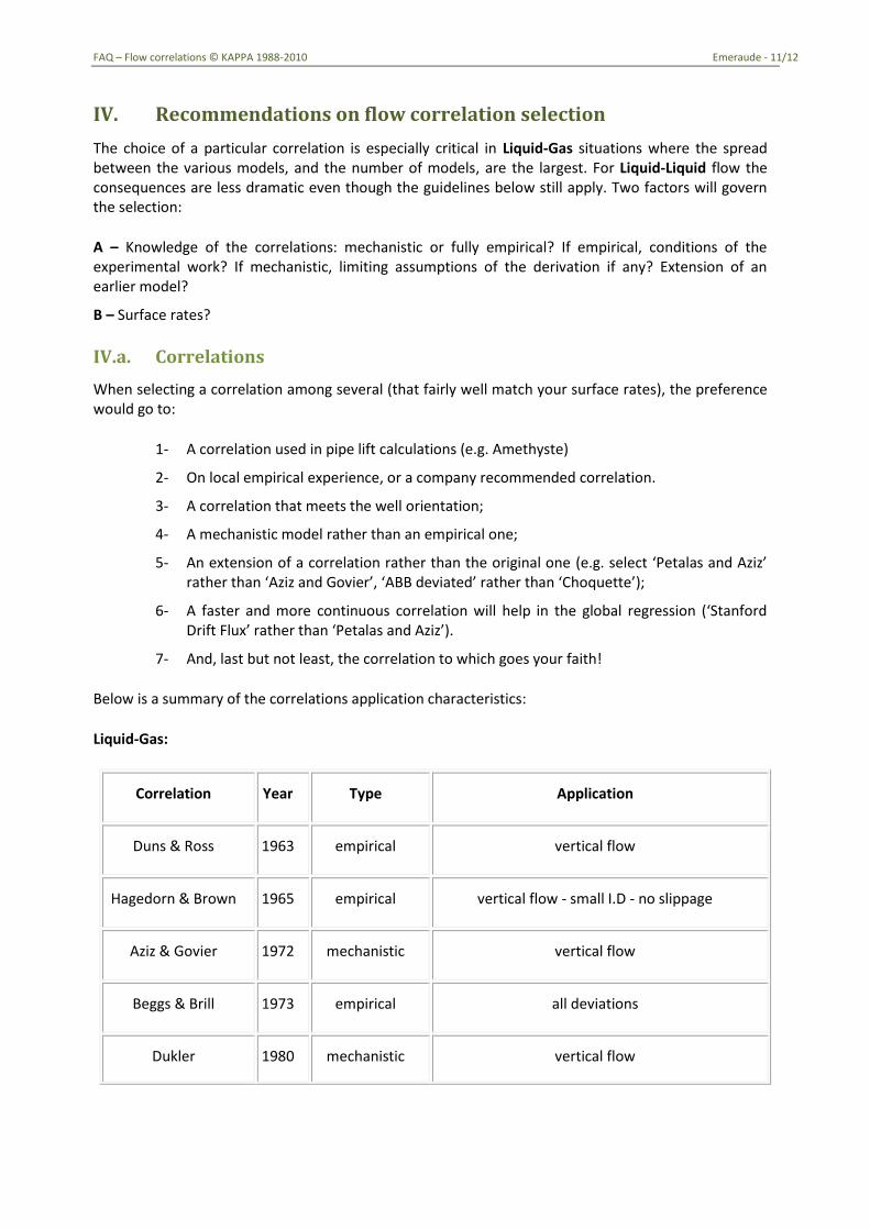
Below is a summary of the correlations application characteristics:

Liquid-Gas:

Correlation Year Type Application

Duns & Ross 1963 empirical vertical flow

Hagedorn & Brown 1965 empirical vertical flow - small I.D - no slippage

Aziz & Govier 1972 mechanistic vertical flow

Beggs & Brill 1973 empirical all deviations

Dukler 1980 mechanistic vertical flow

FAQ – Flow correlations © KAPPA 1988-2010 Emeraude - 12/12

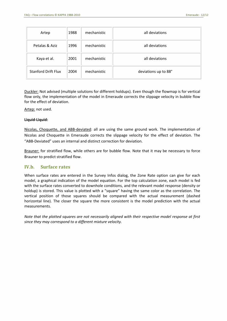
Artep 1988 mechanistic all deviations

Petalas & Aziz 1996 mechanistic all deviations

Kaya et al. 2001 mechanistic all deviations

Stanford Drift Flux 2004 mechanistic deviations up to 88°

Duckler: Not advised (multiple solutions for different holdups). Even though the flowmap is for vertical flow only, the implementation of the model in Emeraude corrects the slippage velocity in bubble flow for the effect of deviation.

Artep: not used.

Liquid-Liquid:

Nicolas, Choquette, and ABB-deviated: all are using the same ground work. The implementation of

Nicolas and Choquette in Emeraude corrects the slippage velocity for the effect of deviation. The

“ABB-Deviated” uses an internal and distinct correction for deviation.

Brauner: for stratified flow, while others are for bubble flow. Note that it may be necessary to force

Brauner to predict stratified flow.

IV.b. Surface rates

When surface rates are entered in the Survey Infos dialog, the Zone Rate option can give for each model, a graphical indication of the model equation. For the top calculation zone, each model is fed with the surface rates converted to downhole conditions, and the relevant model response (density or holdup) is stored. This value is plotted with a “square” having the same color as the correlation. The vertical position of those squares should be compared with the actual measurement (dashed horizontal line). The closer the square the more consistent is the model prediction with the actual measurements.

Note that the plotted squares are not necessarily aligned with their respective model response at first since they may correspond to a different mixture velocity.