Embed Size (px)
Citation preview

Journal of VLSI Signal Processing - Systems for Signal, Image, and Video Technology, X, 1?? (2000)c 2000 Kluwer Academic Publishers, Boston. Manufactured in The Netherlands.
Flexible Independent Component Analysis
SEUNGJIN CHOI
Department of Electrical Engineering
Chungbuk National University, KOREA
Email: [email protected]
ANDRZEJ CICHOCKI
Brain-Style Information Systems Research Group
Brain Science Institute, RIKEN, JAPAN
Email: [email protected]
Warsaw University of Technology, POLAND
SHUN-ICHI AMARI
Brain-Style Information Systems Research Group
Brain Science Institute, RIKEN, JAPAN
Email: [email protected]
;
Editors: M. Van Hulle, M. Niranjan, and T. Adali
Abstract. This paper addresses an independent component analysis (ICA) learning algorithm with exible nonlinearity, so named as exible ICA, that is able to separate instantaneous mixtures of sub-and super-Gaussian source signals. In the framework of natural Riemannian gradient, we employ theparameterized generalized Gaussian density model for hypothesized source distributions. The nonlinearfunction in the exible ICA algorithm is controlled by the Gaussian exponent according to the estimatedkurtosis of demixing �lter output. Computer simulation results and performance comparison with existingmethods are presented.
.1. Introduction
Independent component analysis is a statistical method that plays an important role in lots of applicationssuch as telecommunications [13, 14], feature extraction [8, 9, 17], biomedical signal analysis [37, 32],and data analysis [27] where multiple sensors are involved. The task of ICA is to extract statisticallyindependent components from their linear mixtures without resorting to any prior knowledge. It is knownthat ICA performs blind source separation under mild conditions [24, 3]. In other words, we can recoversources blindly from their linear instantaneous mixtures by a linear transformation that transforms sensorsignals to the output signals that are statistically independent. The demixing system can be viewed as arecognition model in the context of machine learning.

2 S. Choi et al.
Let us assume that the m-dimensional vector of sensor signals, x(t) = [x1(t); : : : ; xm(t)]T is generated
by an unknown linear generative model,
x(t) = As(t); (1)
where s(t) = [s1(t); : : : ; sn(t)]T is the n-dimensional vector whose elements are called sources. The matrix
A 2 IRm�n is called a mixing matrix. It is assumed that source signals fsi(t)g are mutually independentnon-Gaussian signals. The number of sensors, m is greater than or equal to the number of sources, n.The goal of ICA is to recover source signal vector s(t) from the observation vector x(t) without the
knowledge of A nor s(t). To perform this task, we �nd a linear mapping W which forces statisticaldependence among the output signals fyi(t)g to be minimized. It is well known that due to the lackof prior information, there are two indeterminacies in ICA [24]: (1) scaling ambiguity; (2) permutationambiguity. That is, the recovered signal vector y(t) has the form y(t) = P�s(t), whereP is a permutationmatrix and � is some nonsingular diagonal scaling matrix. In many applications, waveforms of sourcesare important factors.Since Jutten and Herault's [33] �rst solution to ICA, several methods have been proposed. They
include robust neural networks approach [23, 22], information maximization [7], natural gradient learning[6, 5], maximum likelihood estimation [41, 36, 40, 11], equivariant algorithms [12], nonlinear principalcomponent analysis (PCA) [34, 39, 31], blind signal extraction [25, 21], cross-cumulants method [18, 38,15]. Mutual information minimization, information maximization, maximum likelihood estimation resultin an identical optimization function (loss function) [11].Typical ICA learning algorithms rely on the choice of nonlinear functions, the optimal form of which
depends on probability distributions of sources. Since probability distributions of sources are not known inadvance in ICA task, we count on the hypothesized density models for sources. Especially for the mixturesof sub- and super-Gaussian sources, the smart choice of nonlinearity is essential. To this end, severalalgorithms have been developed [29, 26, 20, 28, 35]. In the present paper, we employ the generalizedGaussian density model that can approximate both super- and sub-Gaussian sources by the appropriatechoice of Gaussian exponent. Preliminary result was reported in [16]. This is an extended version of ourwork [16] with some new results.This paper is organized as follows. Next section is devoted to give a brief review of natural gradient
based ICA algorithms. In Section .3, the generalized Gaussian density model is introduced. We alsodiscuss the relation between the Gaussian exponent and the kurtosis in the generalized Gaussian distri-bution. In the framework of natural gradient based ICA algorithms, a smart way to select a nonlinearfunction is introduced in Section .4. Practical implementation of the exible ICA algorithms are alsopresented in Section .4. Stability with several di�erent nonlinear functions is studied in Section .5. Com-puter simulation results with arti�cial data and real world data are presented in Section .6. Conclusionswith some discussions are drawn in Section .7
.2. Natural Riemannian Gradient Based ICA Algorithms
Gradient descent learning is a popular method for the purpose of minimizing a given loss function. Whena parameter space (on which a loss function is de�ned) is a Euclidean space with an orthogonal coordinatesystem, the conventional gradient gives the steepest descent direction. However, if a parameter space isa curved manifold (Riemannian space), an orthonormal linear coordinate system does not exist and theconventional gradient does not give the steepest descent direction [1]. Recently the natural gradient wasproposed by Amari [1] and was shown to be eÆcient in on-line learning. See [1] for more details of thenatural gradient. Note that the relative gradient developed independently by Cardoso and Laheld [12]is identical to the natural gradient in the context of ICA. In this section, we brie y review two naturalgradient based ICA algorithms.
Flexible Independent Component Analysis 3
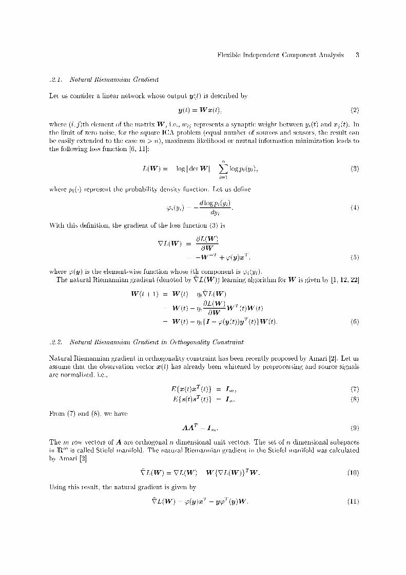
.2.1. Natural Riemannian Gradient
Let us consider a linear network whose output y(t) is described by
y(t) =Wx(t); (2)
where (i; j)th element of the matrixW , i.e., wij represents a synaptic weight between yi(t) and xj(t). Inthe limit of zero noise, for the square ICA problem (equal number of sources and sensors, the result canbe easily extended to the case m > n), maximum likelihood or mutual information minimization leads tothe following loss function [6, 11]:
L(W ) = � log j detW j �
nXi=1
log pi(yi); (3)
where pi(�) represent the probability density function. Let us de�ne
'i(yi) = �d log pi(yi)
dyi: (4)
With this de�nition, the gradient of the loss function (3) is
rL(W ) =@L(W )
@W
= �W�T + '(y)xT ; (5)
where '(y) is the element-wise function whose ith component is 'i(yi).The natural Riemannian gradient (denoted by ~rL(W )) learning algorithm forW is given by [1, 12, 22]
W (t+ 1) = W (t)� �t ~rL(W )
= W (t)� �t@L(W )
@WW T (t)W (t)
= W (t) + �tfI � '(y(t))yT (t)gW (t): (6)
.2.2. Natural Riemannian Gradient in Orthogonality Constraint
Natural Riemannian gradient in orthogonality constraint has been recently proposed by Amari [2]. Let usassume that the observation vector x(t) has already been whitened by preprocessing and source signalsare normalized, i.e.,
Efx(t)xT (t)g = Im; (7)
Efs(t)sT (t)g = In: (8)
From (7) and (8), we have
AAT = Im: (9)
The m row vectors of A are orthogonal n dimensional unit vectors. The set of n dimensional subspacesin IRm is called Stiefel manifold. The natural Riemannian gradient in the Stiefel manifold was calculatedby Amari [2]
~rL(W ) = rL(W )�W frL(W )gTW : (10)
Using this result, the natural gradient is given by
~rL(W ) = '(y)xT � y'T (y)W : (11)

4 S. Choi et al.
Then the learning algorithm for W is given by
W (t+ 1) = W (t)� �t ~rL(W )
= W (t)� �t�'(y(t))xT (t)� y(t)'T (y(t))W (t)
: (12)
It should be noted that when m = n, the matrix W is orthogonal in each iteration step, so this reducesto the following form
W (t+ 1) =W (t)� �t�'(y(t))yT (t)� y(t)'T (y(t))
W (t): (13)
In practice, due to the skew-symmetry of the term '(y(t))yT (t)�y(t)'T (y(t)), decorrelation (or whiten-ing) processing can be performed simultaneously together with separation. With taking this into account,the algorithm becomes Cardoso and Laheld's EASI algorithm [12]
�W (t) = �t�I � y(t)yT (t)� '(y(t))yT (t) + y(t)'T (y(t))
W (t): (14)
The algorithms aforementioned belong to a class of on-line learning algorithms which is based onstochastic approximation. We can also consider the batch versions of the algorithms by estimating timeaverage instead of instantaneous realization. For example, the batch version of the algorithm (14) is givenby
�W (t) = �t�I �
y(t)yT (t)
��'(y(t))yT (t)
�+y(t)'T (y(t))
�W (t); (15)
where < � > denotes the time average operation.
.3. Generalized Gaussian Density Model for Sources
Optimal nonlinear function 'i(yi) is given by (4). However, it requires the knowledge of the probabilitydistributions of sources which are not available to us. A variety of hypothesized density model has beenused. For example, for super-Gaussian source signals, unimodal or hyperbolic-Cauchy distribution model[36] leads to the nonlinear function given by
'i(yi) = tanh(�yi): (16)
Such sigmoid function was also used in [7]. For sub-Gaussian source signals, cubic nonlinear function'i(yi) = y3i has been a favorite choice. For mixtures of sub- and super-Gaussian source signals, accordingto the estimated kurtosis of the extracted signals, nonlinear function can be selected from two di�erentchoices [26]. Several approaches [29, 20, 28, 35] are already available.This paper present a exible nonlinear function derived using generalized Gaussian density model
[20, 19, 16]. It will be shown that the nonlinear function is self-adaptive and controlled by the Gaussianexponent.
.3.1. The Generalized Gaussian Distribution
The generalized Gaussian probability distribution is a set of distributions parameterized by a positivereal number �, which is usually referred to as the Gaussian exponent of the distribution. The Gaussianexponent � controls the \peakiness" of the distribution. The probability density function (PDF) for ageneralized Gaussian is described by
p(y;�) =�
2���1�
�e�j y� j� ; (17)
where �(x) is Gamma function given by
�(x) =
Z 1
0
tx�1e�tdt: (18)

Flexible Independent Component Analysis 5
Note that if � = 1, the distribution becomes the standard \Laplacian" distribution. If � = 2, thedistribution is standard normal distribution (see Figure 1).
−4 −3 −2 −1 0 1 2 3 40
0.1
0.2
0.3
0.4
0.5
0.6
0.7
0.8
0.9
1
y
p(y)
alpha=2alpha=4alpha=1alpha=.8
Fig. 1. The generalized Gaussian distribution is plotted for several di�erent values of Gaussian exponent, � = 0:8; 1; ; 2; 4.
.3.2. The Moments of the Generalized Gaussian Distribution
In order to fully understand the generalized Gaussian distribution, it is useful to look at its moments(specially 2nd and 4th moments which give the kurtosis). The nth moment of the generalized Gaussiandistribution is given by
Mn =
Z 1
�1
ynp(y;�)dy: (19)
If n is odd, the integrand is the product of an even function and an odd function over the whole real line,which integrates to zero. In particular, this implies that the mean of the distribution given in (17) is zeroand it is symmetric about its mean (which means its skewness is zero).The even moments, on the other hand, completely characterize the distribution. In computing these
moments, we use the following integral formula (see pp. 386 in [30])Z 1
0
y��1e��ya
dy =1
a��
1
� ���a
�: (20)
The 2nd moment of the generalized Gaussian distribution is determined by
M2 =
Z 1
�1
y2p(y;�)dy
= 2
Z 1
0
y2�
2���1�
�e�j y� j�dy: (21)
We are integrating only over the positive values of y, we can remove the absolute value in the exponent.Thus
M2 =�
���1�
� Z 1
0
y2e�(y
�)�dy: (22)
Making the substitution z = y�(dy = �dz), we �nd
M2 =��2
��1�
� Z 1
0
z2e�z�
dz: (23)

6 S. Choi et al.
Invoking the integral formula (20), we have
M2 = �2��3�
���1�
� : (24)
In similar way, we can �nd the 4th moment given by
M4 = �4��5�
���1�
� : (25)
In general, the (2k)th moment is given by
M2k = �2k��2k+1�
���1�
� : (26)
.3.3. Kurtosis and Gaussian Exponent
The kurtosis is a nondimensional quantity. It measures the relative peakedness or atness of a distribution.A distribution with positive kurtosis is termed leptokurtic (super-Gaussian). A distribution with negativekurtosis is termed platykurtic (sub-Gaussian). The kurtosis of the distribution is de�ned in terms of the2nd- and 4th-order moments as
�(y) =M4
M22
� 3; (27)
where the constant term �3 makes the value zero for standard normal distribution.For a generalized Gaussian distribution, the kurtosis can be expressed in terms of the Gaussian expo-
nent, given by
�� =��5�
���1�
��2�3�
� � 3: (28)
The plot of kurtosis �� versus the Gaussian exponent � for leptokurtic and platykurtic signals are shownin Figure 2.
0.2 0.4 0.6 0.8 1 1.2 1.4 1.6 1.8 210
−2
10−1
100
101
102
103
104
Gaussian exponent
kurt
osis
Leptokurtic distribution
2 3 4 5 6 7 8 9 1010
−2
10−1
100
101
102
103
104
Gaussian exponent
−ku
rtos
is
Platykurtic distribution
(a) (b)
Fig. 2. The plot of kurtosis �� versus Gaussian exponent �: (a) for leptokurtic signal; (b) for platykurtic signal.

Flexible Independent Component Analysis 7
.4. The Flexible ICA Algorithm
From the parameterized generalized Gaussian density model, the nonlinear function in the algorithm (14)is given by
'i(yi) =d log pi(yi)
dyi
= jyij�i�1sgn(yi); (29)
where sgn(yi) is the signum function of yi.Note that for �i = 1, 'i(yi) in (29) becomes a signum function (which can also be derived from the
Laplacian density model for sources). The signum nonlinear function is favorable for the separation ofspeech signals since natural speeches is often modeled as Laplacian distribution. Note also that for �i = 4,'i(yi) in (29) becomes a cubic function, which is known to be a good choice for sub-Gaussian sources.In order to select a proper value of the Gaussian exponent �i, we estimate the kurtosis of the output
signal yi and select the corresponding �i from the relationship in Figure 2. The kurtosis of yi, �i can beestimated via the following iterative algorithm:
�i(t+ 1) =M4i(t+ 1)
M22i(t+ 1)
� 3; (30)
where
M4i(t+ 1) = (1� Æ)M4i(t) + Æjyi(t)j4; (31)
M2i(t+ 1) = (1� Æ)M2i(t) + Æjyi(t)j2; (32)
where Æ is a small constant, say, 0.01.In general, the estimated kurtosis of demixing �lter output does not exactly match the kurtosis of
original source. However, it provides an idea whether the estimated source is sub-Gassian signal orsuper-Gaussian signal. Moreover, it was shown [11, 3] that the performance of source separation is notdegraded even if the hypothesized density does not match the true density. From these reasons, wesuggest a pratical method where only several di�erent forms of nonlinear functions are used.The kurtosis of platykurtic source does not change much as the Gaussian exponent varies (see Figure 2
(b)), so we use �i = 4 if the estimated kurtosis of yi is negative. The cubic nonlinearity for sub-Gaussiansource is also involved with the kurtosis minimization method [12]. For leptokurtic source, one can seethe kurtosis varies much according to the Gaussian exponent (see Figure 2 (a)). Thus we suggest severaldi�erent values of �i, in contrast to the case of sub-Gaussian source. From our experience, two or threedi�erent values of the Gaussian exponent are enough to handle various super-Gaussian sources. Typicalexamples of nonlinear functions with di�erent values of �i are shown in Figure 3.
.5. Local Stability Analysis
The stability conditions for the algorithm (6) and the algorithm (14) were given by Amari et al. [4]and by Cardoso and Laheld [12], respectively. We �rst brie y review some important results obtained in[4, 12, 10]. Then we investigate the stability e�ect of several nonlinear functions that we have derivedfrom the generalized Gaussian density model. To this end, we focus on the algorithm (14) which employsthe natural gradient in Stiefel manifold.Since the algorithm (14) was derived from the gradient dL = 'T (y)dWx, we need to calculate its
Hessian d2L to check the stability of stationary points. Amari et al. has shown that the calculation ofHessian d2L is relatively easier if the modi�ed di�erential coeÆcient matrix dZ = dWW�1 is employed.Note that the modi�ed di�erential coeÆcient matrix dZ is skew-symmetric in the orthogonality constraint,

8 S. Choi et al.
−6 −4 −2 0 2 4 6
−250
−200
−150
−100
−50
0
50
100
150
200
250
−6 −4 −2 0 2 4 6
−1
−0.5
0
0.5
1
−6 −4 −2 0 2 4 6
−3
−2
−1
0
1
2
3
(a) (b) (c)
Fig. 3. The exemplary shape of nonlinear function 'i(yi): (a) for �i = 4; (b) for �i = 1; (c) for �i = 0:8.
we calculate the Hessian d2L. Using the fact that dZ is skew-symmetric, dL can be written as
dL = 'T (y)dy
= 'T (y)dZy
=Xi;j
'i(yi)dzijyj
=Xi>j
f'i(yi)yj � 'j(yj)yig dzij : (33)
Then the Hessian d2L is calculated as
d2L =Xi>j
Xk
f _'i(yi)dzikykyj � _'j(yj)dzjkykyi
+'i(yi)dzjkyk � 'j(yj)dzikyk g dzij : (34)
Taking into account the normalization constraint (Efy2i g = Efy2j g = 1) and the skew-symmetry, dzij =
�dzji, the expected Hessian at W = A�1 (at desirable solution) is given by
E�d2L
=Xi>j
[E f _'i(yi)g+E f _'j(yj)g
� E f'i(yi)yig �E f'j(yj)yjg] dz2ij ; (35)
where _'i(yi) denotes the derivative of 'i(yi) with respect to yi. From (34), the stability condition isgiven by
�i + �j > 0; (36)
where
�i = E f _'i(yi)g �E f'i(yi)yig : (37)
The stability condition given in (36) coincides with that in [10] but we arrived at this result in theframework of the natural gradient in Stiefel manifold. For each yi, the condition
�i > 0 (38)
is a suÆcient condition for stability.Several di�erent nonlinear functions were suggested in the exible ICA algorithm. Here we investigate
the stability of stationary points of the algorithm (14) for three di�erent cases: (1) �i = 4 for �i < 0; (2)�i = 1; (3) �i = :8 for �i > 0.

Flexible Independent Component Analysis 9
.5.1. Case 1: �i = 4
The choice of �i = 4 was suggested for sub-Gaussian source (�i < 0). The choice of �i = 4 results in thecubic nonlinear function, i.e., 'i(yi) = jyij
2yi. With this selection, one can easily see that the lefthandside of (38) is the kurtosis of yi multiplied by -1. Since yi is sub-Gaussian, the condition (38) is satis�ed.
.5.2. Case 2: �i = 1
With the choice of �i = 1, the generalized Gaussian density (17) becomes Laplacian density, i.e.,
pi(yi) =1
2�ie�j
yi�ij: (39)
The choice of �i = 1 leads to the signum function (hard limiter), i.e.,
'i(yi) = sgn(yi)
=yi
jyij: (40)
In order to calculate the derivative of the signum function, we model it as the sum of two unit stepfunctions, i.e.,
sgn(yi) = u(yi)� u(�yi); (41)
where u(yi) is the unit step function. Then we can calculate the derivative, _'i(yi)
_'i(yi) = 2Æ(yi): (42)
We compute Ef _'i(yi)g
Ef _'i(yi)g =
Z 1
�1
2Æ(yi)1
2�ie�j
yi�ijdyi
=1
�i: (43)
We also compute Ef'i(yi)yig
Ef'i(yi)yig = Efjyijg
= �i: (44)
The normalized constraint, Efy2i g = 1 gives
Efy2i g = 2�2i = 1: (45)
Then, we have �i =q
12 . Note that �i is given by
�i =1� �2i�i
: (46)
Since �i =q
12 , �i is positive for �i > 0.
.5.3. Case 3: �i < 1
For highly peaky sources �i >> 1), it might be desirable to choose the value of �i less than 1. This gives anon-increasing nonlinear function. With this choice, the nonlinear function is singular around the origin.

10 S. Choi et al.
Thus in practical application, for yi 2 [��; �] where � is very small positive number, the correspondingnonlinear function is restricted to have constant values.The variance of yi for the generalized Gaussian distribution is given by
Efy2i g = �2i
��
3�i
���
1�i
� : (47)
From the normalization constraint, Efy2i g = 1, �i has the following value,
�i =
vuuut��
1�i
���
3�i
� : (48)
Besides the region for yi 2 [��; �], we can compute Ef _'i(yi)g and Ef'i(yi)yig given by
Ef _'i(yi)g =
Z 1
�1
(�i � 2)jyij(�i�2)
�i
2�i��
1�i
�e� jyij�i
��ii dyi
=(�i � 2)��i�2i
��
1�i
� �
��i � 1
�i
�;
Ef'i(yi)yig =
Z 1
�1
yijyij(�i�1)sgn(yi)
�i
2�i��
1�i
�e� jyij�i
��ii dyi
=�i�
�i+1i
��
1�i
� 1
�i�
��i + 1
�i
�: (49)
Note that the gamma function �(x) has many singular points especially for x < 0. Thus special care isrequired with the choice of �i < 1. For instance, the choice of �i = 0:5 does not satisfy the condition(38) since �(�1) = 1. For the case of �i = 0:8, one can easily see that the stability condition (38) issatis�ed.
.6. Experimental Results
.6.1. Arti�cial Data
We have performed an experiment with two super-Gaussian sources and two sub-Gaussian sources (seeFigure 4). The kurtoses of sources are -1.2, -1.5, 3.3, 3.6. They were arti�cially mixed using the mixingmatrix A given by
A =
26640:155 0:204 0:431 0:7390:526 0:511 0:404 0:6140:205 0:392 0:306 0:9410:141 0:937 0:656 0:182
3775 : (50)
The Gaussian exponent � can be learned from the estimated kurtosis of the demixing �lter output,through the relation as shown in 2. However, the estimated kurtosis does not exactly match the true one,but its sign does. In practice, only several di�erent values of � can be employed in learning process. Inthis experiment, three di�erent values of Gaussian exponent � were used: (1) � = :8 when the estimatedkurtosis of recovered signal yi(t) is greater than 20; (2) � = 1 when the estimated kurtosis of recoveredsignal is between 0 and 20; (3) � = 4 when the estimated kurtosis of recovered signal is negative.

Flexible Independent Component Analysis 11
As a performance measure, we have used the performance index de�ned by
PI =
nXi=1
( nX
k=1
jgikj2
maxj jgij j2� 1
!+
nX
k=1
jgkij2
maxj jgjij2� 1
!); (51)
where gij is the (i; j)th element of the global system matrix G = WA and maxj gij represents themaximum value among the elements in the ith row vector of G, maxj gji does the maximum value amongthe elements in the ith column vector ofG. When perfect signal separation is carried out, the performanceindex PI is zero. In practice, it is very small number.The synaptic weight matrix W was initialized as the identity matrix. The learning rate �t = 0:0005
was used. Performance comparison was made with extended infomax ICA algorithm [35, 28] where thenonlinear function is switched between �xed � tanh(�) and tanh(�) according to the sign of estimatedkurtosis.Mixtures and recovered signals by the exible ICA algorithm (14) and the extended infomax are
shown in Figures 5, 6, 7. Performance comparison between the exible ICA algorithm and the extendedinfomax algorithm is shown in Figure 8. In Figure 8, the batch versions of both algorithms were usedand prewhitening of data was not performed for both algorithms for fair comparison. One can observethat the exible ICA algorithm gives faster convergence and better performance. Faster convergencemight be due to the natural gradient in Stiefel manifold, i.e., the decorrelation is performed togetherwith separation. Better performance might result from the exible nonlinear function controlled by theGaussian exponent in the exible ICA algorithm in contrast to the �xed nonlinear function employed bythe extended infomax.
0 1000 2000 3000−2
−1
0
1
2
s 1
0 1000 2000 3000−1.5
−1
−0.5
0
0.5
1
1.5
s 2
0 1000 2000 3000−3
−2
−1
0
1
2
3
s 3
0 1000 2000 3000−4
−2
0
2
4
6
s 4
Fig. 4. Original source signals.

12 S. Choi et al.
0 1000 2000 3000−4
−2
0
2
4x 1
0 1000 2000 3000−4
−2
0
2
4
6
x 2
0 1000 2000 3000−5
0
5
x 3
0 1000 2000 3000−4
−2
0
2
4
x 4
Fig. 5. Mixture signals.
0 1000 2000 3000−1
−0.5
0
0.5
1
y 1
0 1000 2000 3000−1.5
−1
−0.5
0
0.5
1
1.5
y 2
0 1000 2000 3000−1.5
−1
−0.5
0
0.5
1
1.5
y 3
0 1000 2000 3000−3
−2
−1
0
1
2
3
y 4
Fig. 6. Recovered signals by the exible ICA algorithm.

Flexible Independent Component Analysis 13
0 1000 2000 3000−4
−2
0
2
4
y 1
0 1000 2000 3000−3
−2
−1
0
1
2
3
y 2
0 1000 2000 3000−4
−2
0
2
4
6
y 3
0 1000 2000 3000−3
−2
−1
0
1
2
3
y 4
Fig. 7. Recovered signals by the extended infomax algorithm.
0 50 100 150 200 250 300 350 400 450 50010
−4
10−3
10−2
10−1
100
101
number of iterations
perf
orm
ance
inde
x
Flexible ICA
Extended Infomax
Fig. 8. The evolution of performance index: solid line is for the exible ICA algorithm and dotted line is for the extendedinfomax algorithm.

14 S. Choi et al.
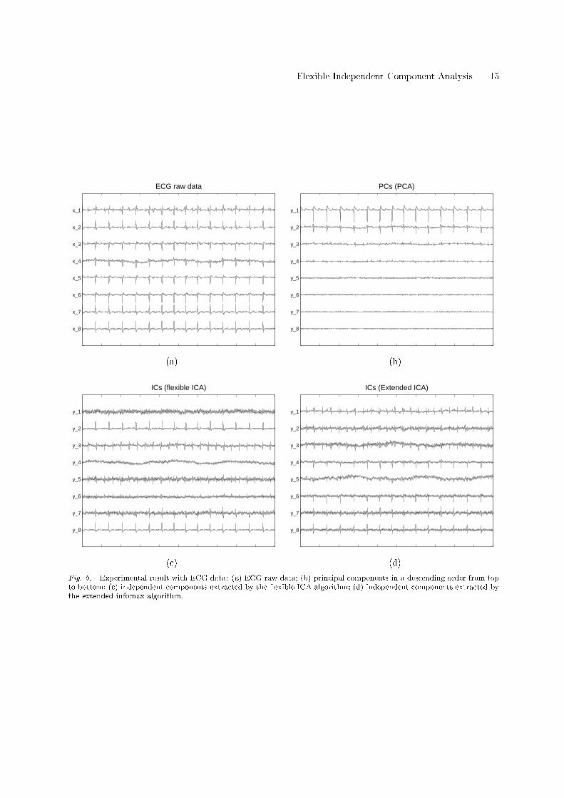
.6.2. Extraction of Fetal ECG source
The ECG data as shown in Figure 9 are the potential recordings during an 8-channel experiment. Only5 seconds of recordings (resampled at 500 Hz) are displayed. In this experiment, the electrodes wereplaced on the abdomen and the cervix of the mother. Abdominal signals measured near fetus are shownin channel 1 to 5. The weak fetal contributions are contained in x1 to x5, although they are not clearlyvisible. The ECG raw data measured through 8 channels are dominated by mother's ECG (MECG).In order to enhance or separate FECG, principal component analysis (PCA) was applied and the result
are shown in Figure 9. The PCA aims at �nding a orthogonal transformation which best models thecovariance structure of the data. First two principal components are MECG, and the third principalcomponent might be FECG, but it is not clear. Since only second-order statistics is used in PCA, it isnot possible to separate MECG and FECG from raw data.The exible ICA algorithm was applied to process the ECG raw data, and the result in shown in Figure
9. The 3rd node output signal y3 corresponds to the FECG signal. Breathing artifact is well extracted atthe 4th output node, y4. The 2nd and 8th node contain the MECG. The rest of extracted signals mightcontain noise contributions. The weak FECG signal was well extracted by the exible ICA algorithm,whereas the PCA had a diÆculty to extract it. We also applied the extended infomax algorithm to thisdata set and the result is shown in Figure 9. It can be observed that the extracted FECG signal was notas clear as the one by the exible ICA algorithm.
.7. Conclusions
We have presented the exible ICA algorithm (in the framework of the natural Riemannian gradient)where self-adaptive nonlinear function is used. For the hypothesized density model, we have employedthe generalized Gaussian distribution that is able to model most uni-modal probability distribution. Thenonlinear function in the algorithm was derived from the generalized Gaussian density. In contrast mostexisting methods, the nonlinear function in our algorithm is controlled by a single parameter (Gaussianexponent). As a practical and simple method, we have suggested several di�erent nonlinear functionsthat resulted from di�erent values of the Gaussian exponent and con�rmed the validity of our approachthrough computer simulations. In addition, rigorous stability analysis for several nonlinear functions wascarried out.
.8. Acknowledgment
This work was supported in part by the Braintech 21, Ministry of Science and Technology, KOREA andin part by BSI, RIKEN, JAPAN.
References
1. S. Amari. Natural gradient works eÆciently in learning. Neural Computation, 10(2):251{276, Feb. 1998.2. S. Amari. Natural gradient for over- and under-complete bases in ICA. Neural Computation, 11(8):1875{1883, Nov.
1999.3. S. Amari and J. F. Cardoso. Blind source separation: Semiparametric statistical approach. IEEE Trans. Signal
Processing, 45:2692{2700, 1997.4. S. Amari, T. P. Chen, and A. Cichocki. Stability analysis of learning algorithms for blind source separation. Neural
Networks, 10(8):1345{1351, 1997.5. S. Amari and A. Cichocki. Adaptive blind signal processing - neural network approaches. Proc. of IEEE, Special Issue
on Blind Identi�cation and Estimation, 86(10):2026{2048, October 1998.6. S. Amari, A. Cichocki, and H. H. Yang. A new learning algorithm for blind signal separation. In D. S. Touretzky, M. C.
Mozer, and M. E. Hasselmo, editors, Advances in Neural Information Processing Systems, volume 8, pages 757{763.MIT press, 1996.
Flexible Independent Component Analysis 15
x_8
x_7
x_6
x_5
x_4
x_3
x_2
x_1
ECG raw data
y_8
y_7
y_6
y_5
y_4
y_3
y_2
y_1
PCs (PCA)
(a) (b)
y_8
y_7
y_6
y_5
y_4
y_3
y_2
y_1
ICs (flexible ICA)
y_8
y_7
y_6
y_5
y_4
y_3
y_2
y_1
ICs (Extended ICA)
(c) (d)
Fig. 9. Experimental result with ECG data: (a) ECG raw data; (b) principal components in a descending order from topto bottom; (c) independent components extracted by the exible ICA algorithm; (d) independent components extracted bythe extended infomax algorithm.
16 S. Choi et al.
7. A. Bell and T. Sejnowski. An information maximisation approach to blind separation and blind deconvolution. NeuralComputation, 7:1129{1159, 1995.
8. A. Bell and T. Sejnowski. Learning the higher-order structure of a natural sound. Network: Computation in NeuralSystems, 7:261{266, 1996.
9. A. Bell and T. Sejnowski. The independent components of natural scenes are edge �lters. Vision Research, 37(23):3327{3338, 1997.
10. J. -F. Cardoso. On the stability of source separation algorithms. In T. Constantinides, S. Y. Kung, M. Niranjan, andE. Wilson, editors, Neural Networks for Signal Processing VIII, pages 13{22, 1998.
11. J. -F. Cardoso. Infomax and maximum likelihood for source separation. IEEE Signal Processing Letters, 4(4):112{114,Apr. 1997.
12. J. -F. Cardoso and B. H. Laheld. Equivariant adaptive source separation. IEEE Trans. Signal Processing, 44(12):3017{3030, Dec. 1996.
13. J. -F. Cardoso and A. Souloumiac. Blind beamforming for non Gaussian signals. IEE Proceedings-F, 140(6):362{370,1993.
14. S. Choi. Adaptive blind signal separation for multiuser communications: An information-theoretic approach. Journalof Electrical Engineering and Information Science, 4(2):249{256, April 1999.
15. S. Choi and A. Cichocki. A linear feedforward neural network with lateral feedback connections for blind sourceseparation. In IEEE Signal Processing Workshop on Higher-order Statistics, pages 349{353, Ban�, Canada, 1997.
16. S. Choi, A. Cichocki, and S. Amari. Flexible independent component analysis. In T. Constantinides, S. Y. Kung,M. Niranjan, and E. Wilson, editors, Neural Networks for Signal Processing VIII, pages 83{92, 1998.
17. S. Choi, A. Cichocki, and S. Amari. Fetal electrocardiogram data analysis using exible independent componentanalysis. In The 4th Asia-Paci�c Conference on Medical and Biological Engineering (APCMBE'99), Seoul, Korea,1999.
18. S. Choi, R. Liu, and A. Cichocki. A spurious equlibria-free learning algorithm for the blind separation of non-zeroskewness signals. Neural Processing Letters, 7:61{68, 1998.
19. A. Cichocki, I. Sabala, and S. Amari. Intelligent neural networks for blind signal separation with unknown number ofsources. In Int. Symp. Engineering of Intelligent Systems, pages 148{154, Tenerife, Spain, 1998.
20. A. Cichocki, I. Sabala, S. Choi, B. Orsier, and R. Szupiluk. Self-adaptive independent component analysis for sub-Gaussian and super-Gaussian mixtures with unknown number of source signals. In International Symposium onNonlinear Theory and Applications, pages 731{734, 1997.
21. A. Cichocki, R. Thawonmas, and S. Amari. Sequential blind signal extraction in order specifed by stochastic properties.Electronics Letters, 33(1):64{65, 1997.
22. A. Cichocki and R. Unbehauen. Robust neural networks with on-line learning for blind identi�cation and blindseparation of sources. IEEE Trans. Circuits and Systems - I: Fundamental Theory and Applications, 43:894{906,1996.
23. A. Cichocki, R. Unbehauen, and E. Rummert. Robust learning algorithm for blind separation of signals. ElectronicsLetters, 43(17):1386{1387, 1994.
24. P. Comon. Independent component analysis, a new concept? Signal Processing, 36(3):287{314, 1994.25. N. Delfosse and P. Loubaton. Adaptive blind separation of independent sources: A de ation approach. Signal Pro-
cessing, 45:59{83, 1995.26. S. C. Douglas, A. Cichocki, and S. Amari. Multichannel blind separation and deconvolution of sources with arbitrary
distributions. In J. Principe, L. Gile, N. Morgan, and E. Wilson, editors, Neural Networks for Signal Processing VII,pages 436{445, 1997.
27. M. Girolami. Hierarchic dichotomizing of polychotomous data - an ICA based data mining tool. In First InternationalWorkshop on Independent Component Analysis and Signal Separation, pages 197{201, 1999.
28. M. Girolami. An alternative perspective on adaptive independent component analysis algorithms. Neural Computation,10(8):2103{2114, Nov. 1998.
29. M. Girolami and C. Fyfe. Generalized independent component analysis through unsupervised learning with emergentBussgang properties. In Proc. ICNN, pages 1788{1791, 1997.
30. I. S. Gradshteyn, I. M. Ryzhik, and A. Je�rey. Table of Integrals, Series, and Products. Academic Press, 1994.31. A. Hyv�arinen and E. Oja. A fast �xed-point algorithm for independent component analysis. Neural Computation,
9:1483{1492, 1997.32. T. P. Jung, C. Humphries, T. Lee, S. Makeig, M. McKeown, V. Iragui, and T. Sejnowski. Extended ICA removes
artifacts from electroencephalographic recordings. In Advances in Neural Information Processing Systems, volume 10,pages 894{900, 1998.
33. C. Jutten and J. Herault. Blind separation of sources, part i: An adaptive algorithm based on neuromimetic architec-ture. Signal Processing, 24:1{10, 1991.
34. J. Karhunen. Neural approaches to independent component analysis. In European Symposium on Arti�cial NeuralNetworks, pages 249{266, 1996.
35. T. W. Lee, M. Girolami, and T. Sejnowski. Independent component analysis using an extended infomax algorithm formixed sub-Gaussian and super-Gaussian sources. Neural Computation, 11(2):609{633, 1999.
36. D. J. C. MacKay. Maximum likelihood and covariant algorithms for independent component analysis. Technical ReportDraft 3.7, University of Cambridge, Cavendish Laboratory, 1996.

Flexible Independent Component Analysis 17
37. S. Makeig, A. Bell, T. P. Jung, and T. Sejnowski. Blind separation of auditory event-related brain responses intoindependent components. Proc. of National Academy of Sciences, 94:10979{10984, 1997.
38. J. P. Nadal and N. Parga. Redundancy reduction and independent component analysis: Conditions on cumulants andadaptive approaches. Neural Computation, 9:1421{1456, 1997.
39. E. Oja. The nonlinear PCA learning rule and signal separation - mathematical analysis. Technical Report A26, HelsinkiUniversity of Technology, Laboratory of Computer and Information Science, 1995.
40. B. Pearlmutter and L. Parra. Maximum likelihood blind source separation: A context-sensitive generalization of ICA.In M. C. Mozer, M. I. Jordan, and T. Petsche, editors, Advances in Neural Information Processing Systems, volume 9,pages 613{619, 1997.
41. D. T. Pham. Blind separation of instantaneous mixtures of sources via an independent component analysis. IEEETrans. Signal Processing, 44(11):2768{2779, 1996.
Seungjin CHOI was born in Seoul, Korea, on October 26, 1964. He received the B.S. and M.S. degrees inelectrical engineering from Seoul National University, Korea, in 1987 and 1989, respectively and the Ph.D degreein electrical engineering from the University of Notre Dame, Indiana, in 1996.After spending the fall of 1996 as a Visiting Assistant Professor in the Department of Electrical Engineering at
University of Notre Dame, Indiana, he was as Frontier Researcher with the Laboratory for Arti�cial Brain Systems,RIEKN in Japan. In August 1997, he joined the School of Electrical and Electronics Engineering at ChungbukNational University where he is currently an Assistant Professor. He has also been an Invited Senior ResearchFellow at Laboratory for Open Information Systems, Brain-style Information Systems Research Group in BrainScience Institute, RIKEN in Japan. His current research interests include brain information processing, statistical(blind) signal processing, independent component analysis, unsupervised learning, and multiuser communications.
Andrzej CICHOCKI was born in Poland on August 1947. He received the M.Sc.(with honors), Ph.D., andHabilitate Doctorate (Dr.Sc.) degrees, all in electrical engineering and computer science, from Warsaw Universityof Technology (Poland) in 1972, 1975, and 1982, respectively.Since 1972, he has been with the Institute of Theory of Electrical Engineering and Electrical Measurements at
the Warsaw University of Technology, where he became a full Professor in 1995.He is the co-author of two international books: MOS Switched-Capacitor and Continuous-Time Integrated
Circuits and Systems (Springer-Verlag, 1989) and Neural Networks for Optimization and Signal Processing (JWiley and Teubner Verlag,1993/94) and author or co-author of more than hundred �fty (150) scienti�c papers.He spent at University Erlangen-Nuernberg (GERMANY) a few years as Alexander Humboldt Research Fellow
and Guest Professor. In 1995-96 he has been working as a Team Leader of the Laboratory for Arti�cial BrainSystems, at the Frontier Research Program RIKEN (JAPAN), in the Brain Information Processing Group directedby professor Shun-ichi Amari. Currently he is head of the laboratory for Open Information Systems in the BrainScience Institute, Riken, Wako-schi, JAPAN.He is reviewer of several international Journals, e.g. IEEE Trans. on Neural Networks, Signal Processing,
Circuits and Systems, Biological Cybernetics, Electronics Letters, Neurocomputing, Neural Computation. Heis also member of several international Scienti�c Committees and the associated Editor of IEEE Transactionon Neural Networks (since January 1998). His current research interests include signal and image processing(especially blind signal/image processing), neural networks and their electronic implementations, learning theoryand algorithms, independent and principal component analysis, optimization problems, circuits and systems theoryand their applications, arti�cial intelligence.

18 S. Choi et al.
Shun-ichi AMARI (Fellow, IEEE) was born in Tokyo, Japan, on January 3, 1936. He graduated from theUniversity of Tokyo in 1958, having majored in mathematical engineering, and he received the Dr.Eng. degreefrom the University of Tokyo in 1963.He was an Associate Professor at Kyushu University, an Associate and then Full Professor at the Department
of Mathematical Engineering and Information Physics, University of Tokyo, and is now Professor-Emeritus at theUniversity of Tokyo. He is the Director of the Brain-Style Information Systems Group, RIKEN Brain ScienceInstitute, Saitama Japan. He has been engaged in research in wide areas of mathematical engineering andapplied mathematics, such as topological network theory, di�erential geometry of continuum mechanics, patternrecognition, mathematical foundations of neural networks, and information geometry.Dr. Amari served as President of the International Neural Network Society, Council member of Bernoulli
Society for Mathematical Statistics and Probability Theory, and Vice President of the Institute of Electrical,Information and Communication Engineers. He was founding Coeditor-in-Chief of Neural Networks. He has beenawarded the Japan Academy Award, the IEEE Neural Networks Pioneer Award, and the IEEE Emanuel R. PioreAward.