FLBEIA a R package to conduct Bio-Economic

Impact assessments using FLR

Dorleta Garcıa, Raul Prellezo, Sonia Sanchez & Marga Andres

April 18, 2013

Abstract

FLBEIA (FL Bio-Economic Impact Assessment) is an R package buildon top of FLR libraries. The purpose of the package is to provide a flex-ible and generic simulation model to conduct Bio-Economic Impact As-sessments of harvest control rule based management strategies under aManagement Strategy Evaluation (MSE) framework. As such, the modelis divided into two main blocks, the operating model (OM) and the man-agement procedure model (MPM). In turn, these two blocks are dividedin 3 components. The OM is formed by the biological, the fleet and thecovariables components and the MPM by the observation, the assessmentand the management advice components.

The model is multistock, multifleet and seasonal and uncertainty isintroduced by means of montecarlo simulation. The algorithm has beencoded in a modular way to ease its checking and to make it flexible. Thepackage provides functions that describe the dynamics of the differentmodel components, under certain assumptions. In each specific modelimplementation the user chooses which of the functions are used. Further-more, if in a specific case study or scenario, for some of the components,the functions provided within FLBEIA do not fulfill the requirements, theuser can code the functions that adequately describe the dynamics of thosecomponents and use existing ones for the rest of the components. As theuser can construct its own model, selecting existing submodels and con-structing new ones, we can define it as a framework more than as a model.The package is still under development but most of its functionalities arealready available. At the moment there are no functions to model trophicinteractions but it is something planed in the short term. Main limitationsof the model are that the stocks must be age structured or aggregated inbiomass (length structure is not allowed) and that spatial dimension is notconsidered explicitly. Spatial characteristics could be modeled assigningstocks and/or fleets/metiers to specific areas.

1

Contents

1 Introduction 4

2 The Concept of BEIA 72.1 Operating Model . . . . . . . . . . . . . . . . . . . . . . . . 7

Biological component: . . . . . . . . . . . . . . . . . 7Fleet component: . . . . . . . . . . . . . . . . . . . . 7Covariates: . . . . . . . . . . . . . . . . . . . . . . . 7Links among and within components: . . . . . . . . 8

2.2 The management procedure model . . . . . . . . . . . . . . 8Observation component: . . . . . . . . . . . . . . . . 8Assessment component: . . . . . . . . . . . . . . . . 8Management advice component: . . . . . . . . . . . 9

3 Running BEIA 93.1 First level function: BEIA . . . . . . . . . . . . . . . . . . . 93.2 Second level functions . . . . . . . . . . . . . . . . . . . . . 10

3.2.1 Biological Component: biols.om . . . . . . . . . . . 103.2.2 Fleets Component: fleets.om . . . . . . . . . . . . 113.2.3 Covariables Component: covars.om . . . . . . . . . 143.2.4 Observation Component: observation.mp . . . . . . 153.2.5 Assessment Component: assessment.mp . . . . . . . 163.2.6 Management Advice Component: advice.mp . . . . 17

3.3 Third level functions . . . . . . . . . . . . . . . . . . . . . . 183.3.1 Population growth functions . . . . . . . . . . . . . . 18

fixedPopulation: Fixed Population function. . . . . 18ASPG: Age Structured Population Growth function. . 18BDPG: Biomass Dynamic Population Growth function. 19

3.3.2 Effort models . . . . . . . . . . . . . . . . . . . . . . 19fixedEffort: Fixed Effort model. . . . . . . . . . . 19SMFB: Simple Mixed Fisheries Behavior. . . . . . . . 19SSFB: Simple Sequential Fisheries Behavior. . . . . . 22MaxProfit.stkCnst: Maximization of profit under

a TAC constraint. . . . . . . . . . . . . . . 233.3.3 Price Models . . . . . . . . . . . . . . . . . . . . . . 24

fixedPrice. . . . . . . . . . . . . . . . . . . . . . . . 24elasticPrice. . . . . . . . . . . . . . . . . . . . . . 24

3.3.4 Capital Models . . . . . . . . . . . . . . . . . . . . . 25fixedCapital. . . . . . . . . . . . . . . . . . . . . . 25SCD: Simple capital Dynamics. . . . . . . . . . . . . 25

3.3.5 Covariables Models . . . . . . . . . . . . . . . . . . . 26fixedCovar. . . . . . . . . . . . . . . . . . . . . . . . 26ssb.get. . . . . . . . . . . . . . . . . . . . . . . . . . 26

3.3.6 Observation Models: Catch and biological parameters 26age2ageDat. . . . . . . . . . . . . . . . . . . . . . . . 26bio2bioDat. . . . . . . . . . . . . . . . . . . . . . . . 28age2bioDat. . . . . . . . . . . . . . . . . . . . . . . . 28

3.3.7 Observation Models: Population . . . . . . . . . . . 28NoObsStock. . . . . . . . . . . . . . . . . . . . . . . . 28

2

perfectObs. . . . . . . . . . . . . . . . . . . . . . . . 28age2agePop. . . . . . . . . . . . . . . . . . . . . . . . 29bio2bioPop. . . . . . . . . . . . . . . . . . . . . . . . 29age2bioPop. . . . . . . . . . . . . . . . . . . . . . . . 29

3.3.8 Observation Models: Abundance Indices . . . . . . . 29ageInd. . . . . . . . . . . . . . . . . . . . . . . . . . 30bioInd. . . . . . . . . . . . . . . . . . . . . . . . . . 30NoObsInd. . . . . . . . . . . . . . . . . . . . . . . . . 30

3.3.9 Observation Model: Fleets . . . . . . . . . . . . . . . 303.3.10 Management Advice Models . . . . . . . . . . . . . . 30

fixedAdvice. . . . . . . . . . . . . . . . . . . . . . . 30annualTAC. . . . . . . . . . . . . . . . . . . . . . . . 30IcesHCR. . . . . . . . . . . . . . . . . . . . . . . . . . 32FroeseHCR. . . . . . . . . . . . . . . . . . . . . . . . 32annexIVHCR. . . . . . . . . . . . . . . . . . . . . . . . 32ghlHCR. . . . . . . . . . . . . . . . . . . . . . . . . . 32aneHCRE. . . . . . . . . . . . . . . . . . . . . . . . . . 32neaMAC_ltmp. . . . . . . . . . . . . . . . . . . . . . . 32

3.4 Fourth level functions . . . . . . . . . . . . . . . . . . . . . 323.4.1 Stock-Recruitment relationships . . . . . . . . . . . 323.4.2 Catch production functions . . . . . . . . . . . . . . 34

CobbDouglasBio. . . . . . . . . . . . . . . . . . . . . 34CobbDouglasAge. . . . . . . . . . . . . . . . . . . . . 35

3.4.3 Costs functions . . . . . . . . . . . . . . . . . . . . . 36TotalCostsPower. . . . . . . . . . . . . . . . . . . . 36

A New FLR - S4 classes 37A.1 FLBDsim class . . . . . . . . . . . . . . . . . . . . . . . . . . 37A.2 FLSRSim class . . . . . . . . . . . . . . . . . . . . . . . . . . 38

B Graphical representation of FLR Objects 39

3

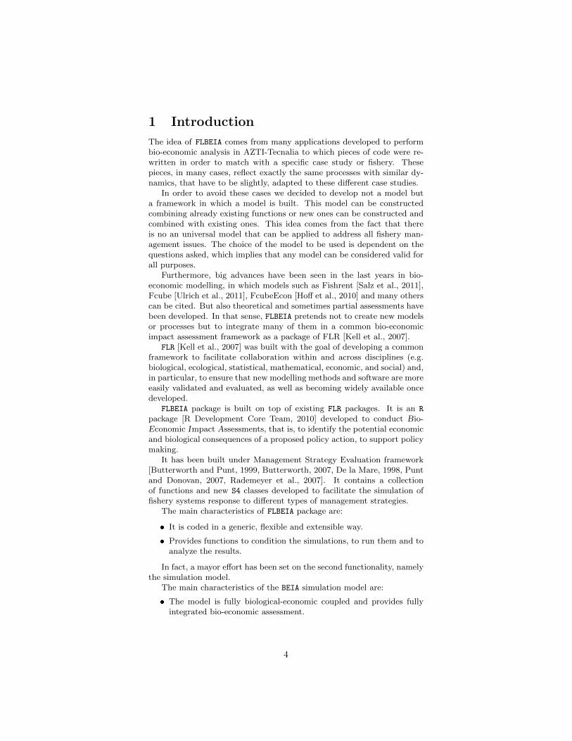
1 Introduction

The idea of FLBEIA comes from many applications developed to performbio-economic analysis in AZTI-Tecnalia to which pieces of code were re-written in order to match with a specific case study or fishery. Thesepieces, in many cases, reflect exactly the same processes with similar dy-namics, that have to be slightly, adapted to these different case studies.

In order to avoid these cases we decided to develop not a model buta framework in which a model is built. This model can be constructedcombining already existing functions or new ones can be constructed andcombined with existing ones. This idea comes from the fact that thereis no an universal model that can be applied to address all fishery man-agement issues. The choice of the model to be used is dependent on thequestions asked, which implies that any model can be considered valid forall purposes.

Furthermore, big advances have been seen in the last years in bio-economic modelling, in which models such as Fishrent [Salz et al., 2011],Fcube [Ulrich et al., 2011], FcubeEcon [Hoff et al., 2010] and many otherscan be cited. But also theoretical and sometimes partial assessments havebeen developed. In that sense, FLBEIA pretends not to create new modelsor processes but to integrate many of them in a common bio-economicimpact assessment framework as a package of FLR [Kell et al., 2007].

FLR [Kell et al., 2007] was built with the goal of developing a commonframework to facilitate collaboration within and across disciplines (e.g.biological, ecological, statistical, mathematical, economic, and social) and,in particular, to ensure that new modelling methods and software are moreeasily validated and evaluated, as well as becoming widely available oncedeveloped.

FLBEIA package is built on top of existing FLR packages. It is an R

package [R Development Core Team, 2010] developed to conduct Bio-Economic Impact Assessments, that is, to identify the potential economicand biological consequences of a proposed policy action, to support policymaking.

It has been built under Management Strategy Evaluation framework[Butterworth and Punt, 1999, Butterworth, 2007, De la Mare, 1998, Puntand Donovan, 2007, Rademeyer et al., 2007]. It contains a collectionof functions and new S4 classes developed to facilitate the simulation offishery systems response to different types of management strategies.

The main characteristics of FLBEIA package are:

It is coded in a generic, flexible and extensible way.

Provides functions to condition the simulations, to run them and toanalyze the results.

In fact, a mayor effort has been set on the second functionality, namelythe simulation model.

The main characteristics of the BEIA simulation model are:

The model is fully biological-economic coupled and provides fullyintegrated bio-economic assessment.

4

The model deals with multi-species, multi-fleet and multi-metier sit-uations.

The model can be run using seasonal steps (smaller or equal to oneyear).

It is generic, flexible and extensible.

Uncertainty can be introduced in almost any of the parameters used.

A conceptual diagram of the model is shown in figure 1. The simula-tion is divided in two main blocks: the Operating Model (OM) and theManagement Procedure Model (MPM). The OM is the part of the modelthat simulates the real dynamics of the fishery system and the MPM isthe part of the model that simulates the whole management process.

Figure 1: Conceptual diagram of BEIA

The OM has three components that can interact among themselves:

1. The biological populations or stocks.

2. The fleets.

3. The covariables. They can be of any nature; environmental, eco-nomical or technical.

The MPM has also three components:

1. The data collected from the OM.

2. The observed population obtained through the application of a setof assessment models to the observed data.

5

3. The management advice obtained from the application of harvestcontrol rules (HCR) to the observed populations.

The model is built modularly with a top-down structure that has, atleast, four levels:

1. In the first level (top level), there is only one function, BEIA function.It calls the functions on the second level in a determined order and itlinks the main components (stocks, fleets, covariates, data, observedpopulation and management advice) of the OM and MPM.

2. The functions in the second level correspond with the componentsin the figure 1. The OM components project the objects one sea-son forward: biols.om projects the stocks, fleets.om projects thefleets and covars.om projects the covariables. The MPM compo-nents generate the objects necessary to produce the managementadvice, they generate the objects based on OM objects and theyoperate at most once a year: observation.mp generates the data,assessment.mp generates the observed population and advice.mp

generates the management advice. They take the input objects andreturns only those related to the component they belong to.

3. The functions in the third level define the specific dynamics of eachcomponent and they are chosen by the user in each simulation. Theyare always called by a second level function and in some cases theycall fourth level functions, for example a function that describes thedynamics of an age structured population can call a stock recruit-ment function. In this way, a function used to describe age struc-tured populations can be combined with different stock recruitmentrelationships.

4. The functions in the fourth level are called by functions in the thirdlevel and are used to model the most basic processes in the simula-tion. They are coded as a function and selected by the user becauseit could be interesting to use the same third level function togetherwith different fourth level functions, as in the case of age structuredpopulation and stock recruitment functions.

This top down structure allows us to avoid the classical structure ofseparated biological and economic (and social) modules (that could beintegrated or not). When designing the model, we can think out onlyat what level do we want to include a particular characteristic, and thisdecision is independent of being a biological or an economic characteristic.

FLBEIA is prepared to incorporate new third and lower level com-ponents or to modify them, while first and second level ones are fixed.Changing first or second level functions would imply a different approach,but existing third and lower level functions would be usable.

In the next two sections, BEIA’s conceptual model and its specifica-tions will be explained. The conceptual model will characterize the maincomponents as well as the feedbacks and loops among them. The modelspecification, will describe the components, the functions by level, the cur-rently available third and four level functions and how to use them withinthe FLBEIA package.

6

2 The Concept of BEIA

As commented above the simulation model has been divided in two mainblocks, the Operating Model (OM) and the Management Procedure Model(MPM). This division is part of the requirements of the MSE approach,that is, mathematical representations of the real world (OM), the observedworld (MPM) and the interactions between them.

2.1 Operating Model

The OM is the part of the model that simulates the real dynamics of thefishery system. It is divided in three components or operating models, thebiological operating model, the fleets operating model, and the covariablesoperating model.

It runs in seasonal steps, projecting the components in each step.Firstly, the biological component is updated, secondly the fleet compo-nent and finally the covariable component.

Biological component: The biological component simulates the pop-ulation dynamics of the biological populations, the stocks. The numberof populations is, in principle, unlimited. The limitation could come frommemory problems with R and/or the operating system. The stocks canbe described as age structured populations or as biomass dynamic pop-ulations, length structured populations models are not supported by thesimulation algorithm. Each stock can follow a different population dy-namics model and is projected independently. It does not mean thatthere cannot interdepend between them but the order in which these bi-ological components are updated has to be decided and it will affect theresults obtained.

Fleet component: The fleet component simulates the behaviour anddynamics of the individual fleets. As the number of the stocks, the numberof fleets is in principle unlimited. The limitation could come from memoryproblems with R and/or the operating system used. The activity of thefleets is divided into metiers. The metiers are formed by trips that sharethe same catchability for all the stocks caught. Fishing effort of the fleetsand their effort share among metiers are independently updated for eachfleet in each season.

There is also defined a capital dynamics that annually updates thecapacity and/or catchability of the fleets according to their economic per-formance, independently for each fleet.

Covariates: This part of the model is intended to incorporate all thevariables that are not part of the biological or fleet components and thataffect any of the operating model components or the management process.The number of covariates is, in principle, unlimited. The limitation couldcome from memory problems with R and/or the operating system used.

7

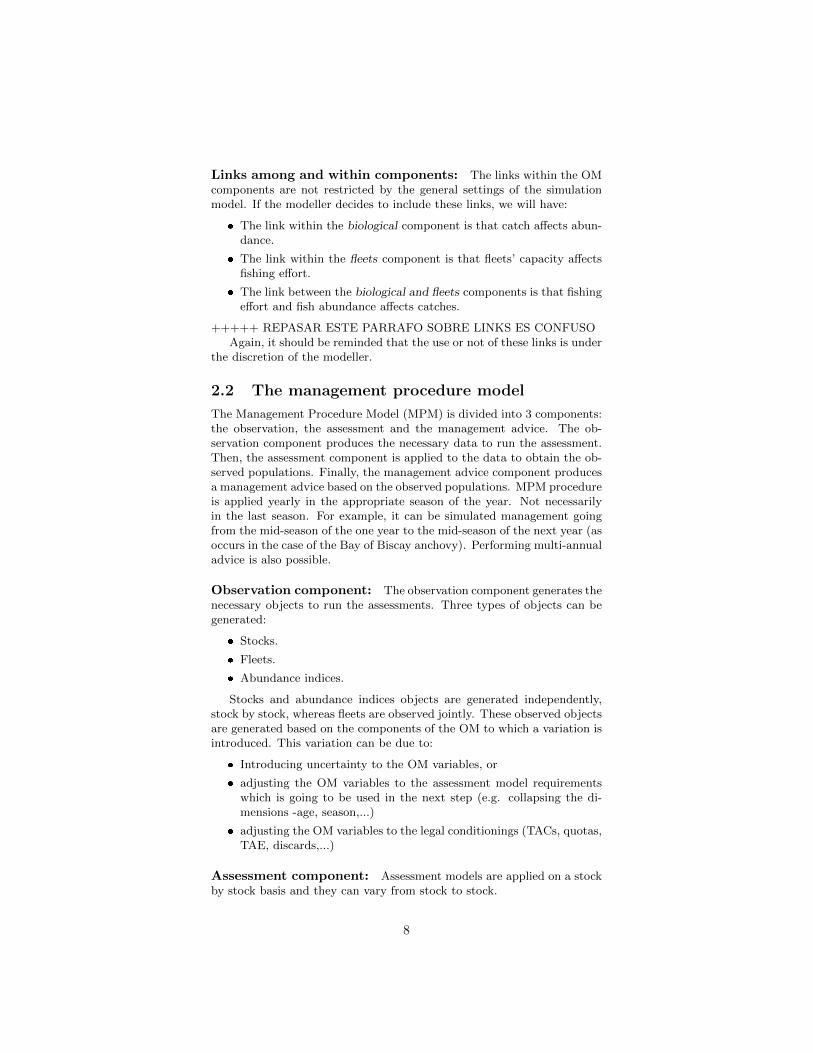
Links among and within components: The links within the OMcomponents are not restricted by the general settings of the simulationmodel. If the modeller decides to include these links, we will have:

The link within the biological component is that catch affects abun-dance.

The link within the fleets component is that fleets’ capacity affectsfishing effort.

The link between the biological and fleets components is that fishingeffort and fish abundance affects catches.

+++++ REPASAR ESTE PARRAFO SOBRE LINKS ES CONFUSOAgain, it should be reminded that the use or not of these links is under

the discretion of the modeller.

2.2 The management procedure model

The Management Procedure Model (MPM) is divided into 3 components:the observation, the assessment and the management advice. The ob-servation component produces the necessary data to run the assessment.Then, the assessment component is applied to the data to obtain the ob-served populations. Finally, the management advice component producesa management advice based on the observed populations. MPM procedureis applied yearly in the appropriate season of the year. Not necessarilyin the last season. For example, it can be simulated management goingfrom the mid-season of the one year to the mid-season of the next year (asoccurs in the case of the Bay of Biscay anchovy). Performing multi-annualadvice is also possible.

Observation component: The observation component generates thenecessary objects to run the assessments. Three types of objects can begenerated:

Stocks.

Fleets.

Abundance indices.

Stocks and abundance indices objects are generated independently,stock by stock, whereas fleets are observed jointly. These observed objectsare generated based on the components of the OM to which a variation isintroduced. This variation can be due to:

Introducing uncertainty to the OM variables, or

adjusting the OM variables to the assessment model requirementswhich is going to be used in the next step (e.g. collapsing the di-mensions -age, season,...)

adjusting the OM variables to the legal conditionings (TACs, quotas,TAE, discards,...)

Assessment component: Assessment models are applied on a stockby stock basis and they can vary from stock to stock.

8

Management advice component: The management advice com-ponent produces a set of indicators (determined by the user) useful forpolicy making. The management advice is produced based on the outputobtained from the observation and assessment components. The advice isfirst applied at single stock level and then (after that) it can be appliedat fleet level.

3 Running BEIA

3.1 First level function: BEIA

The simulations are run using BEIA function. This function is a multistock,multifleet and seasonal simulation algorithm coded in a generic, flexibleand extensible way. It is generic in the sense that can be applied to anycase study that fit into the model restrictions. The algorithm is madeup by third and fourth level functions specified by the user. Apart fromexisting functions new ones can be defined and used if necessary. This isthe reason to define it as flexible and extensible.

To determine the simulation the third- and fourth-level functions mustbe specified. For this end, in the main function call, there is a control ar-gument associated to each second level function. These control argumentsare lists which include, apart from the name of the functions to be used inthe simulations, any extra argument needed by those functions that arenot contained in the main arguments.BEIA function is called as follows:

BEIA(biols, SRs, BDs, fleets, covars, indices, advice,

main.ctrl, biols.ctrl, fleets.ctrl, covars.ctrl,

obs.ctrl, assess.ctrl, advice.ctrl)

Main arguments:

biols : An FLBiols object. The object must be named and the namesmust coincide with those used in SRs object, BDs object and catches

slots within FLFleetExts object.

SRs : A list of FLSRsim objects. This object is a simulation version ofthe original FLSR object. The object must be named and the namesmust coincide with those used in FLBiols object. For details on thisobject see the figure in the annex.

BDs : A list of FLBDsim objects. This object is similar to FLSRs object butoriented to simulate population growth in biomass dynamic popu-lations. The object must be named and the names must coincidewith those used in FLBiols object. For details on this object see thefigure in the annex.

fleets : An FLFleetExts object. This object is almost equal to the orig-inal FLFleet object but the FLCatch object in catch slot has beenreplaced by FLCatchExt object. The difference between FLCatch andFLCatchExt objects is that FLCatchExt has two extra slots alpha andbeta used to store Cobb-Douglas production function parameters, αand β, [Cobb and Douglas, 1928, Clark, 1990]. α corresponds with

9

effort’s exponent and β with that of biomass. The FLFleetExts ob-ject must be named and the names used must be consistently usedin the rest of the arguments. For details on this object see the figurein the annex.

covars : An FLQuants object. This object is not used in the most basicconfiguration of the algorithm. Its content is totally dependent onthe third or lower level functions that make use of it.

indices : A list of FLIndices objects. Each element in the list corre-sponds with one stock. The list must be named and the names mustcoincide with those used in FLBiols object.

advice : A list. The class and content of its elements depends on func-tions used in fleet.om to simulate fleets’ effort and the functionsused to produce advice in advice.mp.

Control arguments:

main.ctrl : Controls the behavior of the main function, BEIA.

biols.ctrl : Controls the behavior of the second level function biols.om.

fleets.ctrl : Controls the behavior of the second level function fleets.om.

covars.ctrl : Controls the behavior of the second level function co-

vars.om.

obs.ctrl : Controls the behavior of the second level function observa-

tion.mp.

assess.ctrl : Controls the behavior of the second level function assess-

ment.mp.

advice.ctrl : Controls the behavior of the second level function ad-

vice.mp.

3.2 Second level functions

3.2.1 Biological Component: biols.om

The call to the function within BEIA is done as:

biol.om(biols, fleets, SRs, BDs, covars, biols.ctrl, year,

season)

This function projects the stocks one season forward. The projectionis done independently stock by stock by the third level function specifiedfor each stock in biols.ctrl object. Currently, there are three popula-tion dynamics functions implemented, one corresponding to age structuredpopulations, ASPG, the second one to biomass dynamic populations, BDPGand another one to fixed populations given as input, fixedPopulation.These functions do not include predation among stocks, but this kind ofmodels could be implemented and used in the algorithm if necessary.Control arguments:

biols.control : This argument is a list which contains the necessaryinformation to run the third level functions that are called by bi-

ols.om. The elements depend on the third and lower level functions

10

used to describe the dynamics of the stocks. The list must containat least one element per stock and the name of the element mustcoincide exactly with the name used in biols argument so it can beused to link the population with its dynamics model. At the sametime, each of these elements must be a list with at least one element,dyn.model, which specifies the name of the function used to describepopulation dynamics.

When only ASPG and/or BDPG functions are used the biols.ctrl

object is just a list with one element per stock. And these elementsare lists with just one element, dyn.model, specifying the name ofthe function used to describe population dynamics, ASPG, BDPG orfixedPopulation. For example:

> biols.ctrl

$NHKE

$NHKE$dyn.model

[1] "ASPG"

$CMON

$CMON$dyn.model

[1] "BDPG"

$FAKE

$FAKE$dyn.model

[1] "ASPG"

3.2.2 Fleets Component: fleets.om

The call to fleets.om function within BEIA is done as:

fleets.om(fleets, biols, covars, advice,

fleets.ctrl, year, season)

This function projects the fleets one season forward. The main ar-gument, fleets, is an object of class FLFleetsExt (for more detail seesection 3.1)

The function is divided in three processes related to fleet dynamics:the effort model, the price model and the capital model. Effort and capitalmodels are fleet specific, whereas price model is fleet and stock specific.First, fleets.om calls the effort model and it updates the slots relatedto effort and catch. The effort models are called independently fleet byfleet. Then, fleets.om calls the price model in fleet by fleet and stock bystock basis. The price model updates the price slot in the fleets object.Finally, the function calls the capital model, but the call is done in thelast season of the year. Thus, investment and disinvestment is only doneannually. The capital model is called independently fleet by fleet.

Effort model: This part of the model simulates the tactical behaviourof the fleet every season and iteration. In each time step and itera-tion, the effort exerted by each individual fleet and its effort-share

11

among metiers is calculated depending on the stock abundance, man-agement restrictions or others. After that, the catch produced bythe combination of effort and effort-share is calculated and dis-

cards, discards.n, landings, landings.n slots are filled. Othervariables stored in fleets.ctrl could also be updated here, for ex-ample quota.share, as a result of the exerted effort.

The effort model is specified at fleet level, so each fleet can followa different effort model. At the moment there are 4 functions avail-able, fixedEffort, SMFB, SSFB and MaxProf.StkCnst. To writenew functions for effort, it must be taken into account that the in-put arguments must be found among fleets.om function argumentsand that the output must be a list with updated FLFleetsExt andfleet.ctrl objects, i.e.:

list(fleets = my_fleets_obj, fleet.ctrl = my_fleet.ctrl_obj)

Price Model: The price model updates the price-at-age at stock, metierand fleet level in each time step and iteration.

At the moment, there are 2 functions available, fixedPrice andelasticPrice. To write new functions for price it must be taken intoaccount that the input arguments must be found among fleets.om

function arguments and that the output must be a list with an up-dated FLFleetsExt object.

Capital Model: This module is intended to simulate the strategic be-haviour of the fleets, namely, the investment and disinvestment dy-namics. The model is applied at fleet level and in an annual basisand can affect fleets’ capacity and catchability. Catchability couldbe modified through investment in technological improvement andcapacity as a result of an increase (investment) or decrease (disinvest-ment) in the number of vessels. Changes in fleets’ capacities couldproduce a variation in quota share among fleets, for example. Thus,the corresponding change would have to be done in fleets.ctrl

object.

At the moment, there are 2 functions available, fixedCapital andSCD. To write new functions for capital dynamics, as for effort andprice, it must be taken into account that the input arguments mustbe found among fleets.om function arguments and that the outputmust be a list with updated FLFleetsExt and fleets.ctrl objects.

Control arguments:

fleets.ctrl : The most simple example of fleet dynamics model andhence the most simple fleets.ctrl object correspond with the modelwhere all the parameters in fleets object are given as input andmaintained fixed within the simulation. This is obtained using thethird level functions, fixedEffort, fixedPrice and fixedCapital

which do not need any extra arguments. In the case of two fleets,FL1 and FL2, where FL1 catches 3 stocks, ST1, ST2 and ST3 and FL2

catches ST1 and ST3 stocks, the fleets.ctrl could be created usingthe following code:

12

>fleets.ctrl <- list()

# The fleets

>fleets.ctrl[['FL1']] <- list()

>fleets.ctrl[['FL2']] <- list()

# Effort model per fleet.

>fleets.ctrl[['FL1']]$effort.dyn <- 'fixedEffort'

>fleets.ctrl[['FL2']]$effort.dyn <- 'fixedEffort'

# Price model per fleet and stock.

>fleets.ctrl[['FL1']][['ST1']]$price.dyn <- 'fixedPrice'

>fleets.ctrl[['FL1']][['ST2']]$price.dyn <- 'fixedPrice'

>fleets.ctrl[['FL1']][['ST3']]$price.dyn <- 'fixedPrice'

>fleets.ctrl[['FL2']][['ST1']]$price.dyn <- 'fixedPrice'

>fleets.ctrl[['FL2']][['ST3']]$price.dyn <- 'fixedPrice'

# Capital model by fleet.

>fleets.ctrl[['FL1']]$capital.dyn <- 'fixedCapital'

>fleets.ctrl[['FL2']]$capital.dyn <- 'fixedCapital'

> fleets.ctrl

$FL1

$FL1$effort.dyn

[1] "fixedEffort"

$FL1$ST1

$FL1$ST1$price.dyn

[1] "fixedPrice"

$FL1$ST2

$FL1$ST2$price.dyn

[1] "fixedPrice"

$FL1$ST3

$FL1$ST3$price.dyn

[1] "fixedPrice"

$FL1$capital.dyn

[1] "fixedCapital"

$FL2

$FL2$effort.dyn

[1] "fixedEffort"

13

$FL2$ST1

$FL2$ST1$price.dyn

[1] "fixedPrice"

$FL2$ST3

$FL2$ST3$price.dyn

[1] "fixedPrice"

$FL2$capital.dyn

[1] "fixedCapital

3.2.3 Covariables Component: covars.om

covars.om projects covars object one season forward. covars object isa named list and the class and dimension of each element will depend onthe function used to project it into the simulation.

The call to covars.om function within BEIA is done as:

covars.om(biols, fleets, covars, advice,

covars.ctrl, year, season)

Internally, for each element in the covars list, it calls to the third levelfunctions specified in the covars.ctrl object. At the moment, there exist2 third level functions: fixedCovar, which is used to work with variablesthat are input parameters not updated within the simulation and ssb.get,which is used to get the real abundance of one of the simulated stocks.

This way of working could be useful, for example, for environmentalvariables such as sea surface temperature that could affect catchability orrecruitment in the fleet and biological operating models respectively andthat are external to fishery system.

A covariable with a non-trivial dynamics could be the abundance ofcertain animal which is not commercially exploited by the fleet, but whichabundance affects the natural mortality of any of the exploited stocks.In this case, 2 extra functions will be needed, the function that definesthe dynamics of the covariable and the function that models the naturalmortality of the stock as a function of the abundance of the animal. Thefirst function should be declared in covars.ctrl argument and the formerone in biols.ctrl argument as a stock dynamics model.Control arguments:

covars.ctrl : This argument is a named list with one element per co-variable and the names of the list must match those used to namethe covars object. Each of the elements is, at the same time, a listwith, at least, one element, dyn.model, which defines the dynamicsof the covariable in question.

14

3.2.4 Observation Component: observation.mp

The observation component generates the necessary data to run the as-sessment models. The main function is observation.mp and it calls thirdlevel functions which generate 3 possible objects, a FLStock, a FLIndices

or a FLFleetsExt object. The FLStock and FLIndices objects are gener-ated independently for each stock and the FLFleetsExt object jointly forall the fleets.

The call to observation.mp function within BEIA is done as:

observation.mp(biols, fleets, covars, indices, advice,

obs.ctrl, year)

The output of observation.mp is a list with 3 elements. The firstelement, stocks, is a named list with one element per stock and its namescorrespond with those used in the biols object. The elements of thestocks list are of class FLStock or NULL, if a FLStock is not needed torun the assessment. The second element, indices, is a named list withone element per stock and its names correspond with those used in biols

object. The elements of the indices list are of class FLIndices or NULL,if a FLIndices is not needed to run the assessment. The third element,fleets.obs, is an observed version of the original fleets object. Thesegmentation of the fleet in the observed version would be different to thereal one (in this moment there is no third level function implemented togenerate observed fleets). +++++ LO VAMOS A IMPLEMENTAR ACORTO PLAZO O CAMBIAMOS LA REDACCION DEL TEXTO?

As the management process is currently run in a yearly basis, theunit and season dimensions are collapsed in all the observed objects.Moreover, if the management process is being conducted at the end ofyear y the observed objects extend up to year y-1, whereas they extendup to year y in the cases when management process is conducted in anyother season as it happens in reality.Control arguments:

obs.ctrl : This argument is a list with one element per stock. If fleetswere observed the object should have also one element per fleet butas at the moment there are no functions that provide observed ver-sion of FLFleetsExt object this option is not described here. Theobs.ctrl object must be a named list where the names used corre-spond with those used in the FLBiols object. Each stock elementis, at the same time, a list with two elements (stockObs and in-

dicesObs) and this two elements are once again lists. A schemeof obs.ctrl object is presented in Figure 2. +++++ REVISARFIGURA (notacion incorrecta)

The stockObs element is a list with the arguments necessary to runthe third level function used two generate the FLStock object. Inthe list there must be at least one element, stockObsModel, with thename of the third level function that will be used two generate theFLStock object. If it is not required to generate a FLStock objectNoObject should be assigned to stockObsModel argument and thisfunction will return the NULL object.

15

Figure 2: obs.ctrl object scheme

The indicesObs element is a list with one element per index in theFLIndices object. Each element of the list is, at the same time,a list with the arguments necessary to run the third level functionused to generate the FLIndex object. In the list there must be atleast one element, indexObsModel, with the name of the third levelfunction that will be used two generate the FLIndex object. If itis not required to generate a FLIndices object indicesObs elementwill be set equal to NoObject instead of a list and this will returnthe NULL object instead of a FLIndices for the corresponding stock.

3.2.5 Assessment Component: assessment.mp

The assessment component applies an existing assessment model to thestock data objects generated by the observation model (FLStock andFLIndices). The assessment models are applied stock by stock, inde-pendently.

The call to assessment.mp function within BEIA is done as follows:

16

assessment.mp(stocks, fleets.obs, indices, assess.ctrl,

datayr)

The output of the function is a list of FLStocks with harvest, stock.nand stock slots updated. Within FLBEIA no new assessment models areprovided, but the models already available in FLR can be used.Control arguments:

assess.ctrl : This argument is a named list with one element per stock,where the names must coincide with those used in biols object.The elements must have at least one element, assess.model, whichdefines the name of the assessment model to be used for each stock.Furthermore, if the assessment model to be used is non-trivial (notNoAssessment), the list must contain a second argument control

with the adequate control object to run the assessment model.

3.2.6 Management Advice Component: advice.mp

The Management Advice component generates an advice based on theoutput of assessment and/or observation components.

The call to advice.mp function within BEIA is done as follows:

advice.mp(stocks, fleets.obs, indices, covars, advice,

advice.ctrl, year, season

First, the advice is generated stock by stock, independently. Later afunction that generates advice based on the single stock advices, observedfleets and others could be applied, FCube like approaches [Ulrich et al.,2011]. The output of the function is an updated advice object.

Depending on the structure of the third level functions used to generateadvice and to simulate fleet dynamics, the advice could be an input advice(effort, temporal closures, spatial closures -implicitly through changes incatchability-...) or an output advice (catch).

advice object : The structure of this object is open and it is completelydependent on the third level functions used to describe fleet dynam-ics and to generate the advice. For example, if SMFB and annualTAC

are used to describe fleet dynamics and generate the advice respec-tively, advice is a list with two elements, TAC and quota.share. TACis an annual FLQuant with the quant dimension used to store stockspecific TACs and, quota.share is a named list with one elementper stock being the elements FLQuant-s with quant dimension usedto store fleet specific annual quota share.

Control arguments:

advice.ctrl : This argument is a named list with one element per stockand one more element for the whole fleet. The names must coincidewith those used to name biols object and the name of the extraargument must be fleets. The elements of the list are, at the sametime, lists with at least one element, HCR, with the name of the modelused to generate the single stock and fleet advice depending on thecase.

17

3.3 Third level functions

3.3.1 Population growth functions

fixedPopulation: Fixed Population function. In this functionall the parameters are given as input, because there is not any populationdynamics simulated.

ASPG: Age Structured Population Growth function. The func-tion ASPG describes the evolution of an age structured population usingan exponential survival equation for existing age classes and a stock-recruitment relationship to generate the recruitment. The recruitmentcan occur in one or more seasons. However, the age is measured in inte-ger years and the seasonal cohorts are tracked separately. The seasonalcohorts and their corresponding parameters are stored in the ’unit (u)’dimension of the FLQuant-s. And all the individuals move from one agegroup to the following one in the 1st of January. Thus, being φ the recruit-ment function, RI the reproductive index, N the number of individuals,M the natural mortality, C the catch, a0 the age at recruitment, s0 theseason when the recruitment was spawn, and a, y, u, s the subscripts forage, year, unit and season respectively, the population dynamics can bewritten mathematically as:

If s = 1,

Na,y,u,1 =

φ (RIy=y−a0,s=s−s0) a = a0

(Nia · e−Mia

2 − Cia) · e−Mia

2 a0 < a < A

(NiA−1 · e−

MiA−12 − CiA−1) · e−

MiA−12 +

(NiA · e−

MiA2 − CiA) · e−

MiA2 a = A,

(1)where ia = (a − 1, y − 1, u, ns), iA−1 = (A − 1, y − 1, u, ns) and iA =

(A, y − 1, u, ns).If s > 1,

Na,y,u,s =

φ (RIy=y−a0,s=s−s0) a = a0

(Nia · e−Mia

2 − Cia) · e−Mia

2 a0 < a < A(2)

where ia = (a, y, u, s− 1)And the reproductive index RI is given by:

RIy−a0,s =∑a

∑u

(N · wt · fec · spwn)a,y−a0,u,s (3)

where wt is the mean weight, fec +++++ and spwn +++++.+++++ DORLETA: por favor revisa la formula anterior (e.g. SSB =∑a

∑u(N ·wt · fec · exp− (M ·Mspwn +F ·Fspwn))), otros ejemplos?????

Depending on what is stored in the fec slot, RI can be SSB or any otherreproductive index of the population. The stock-recruitment relationshipφ is specified in the model slot of corresponding FLSRsim object. FLSRsim

object enables modeling a great variety of stock-recruitment relationshipsdepending on its functional form and seasonal dynamics.

18

BDPG: Biomass Dynamic Population Growth function. Thefunction BDPG describes the evolution of a biomass dynamic population,i.e. a population with no age, stage or length structure. The population isaggregated in biomass, B, and the growth of the population, g is a functionof the current biomass and the catch C. The model is mathematicallydescribed in equation 4:

Bs,y =

Bs−1,y + g(Bs−1,y)− Cs−1,y s 6= 1,Bns,y−1 + g(Bns,y−1)− Cns,y−1 s = 1.

(4)

NOTATION!!! Because BEIA is seasonal the equation depends on sea-son. The growth model g and its parameters are specified, respectively, inthe model and params slot of corresponding FLBDsim class. Currently onlyPella and Tomlinson model [Pella and Tomlinson, 1969] is implementedto model growth, but new models can be defined if needed. The followingparameterization of the growth model has been implemented:

g(B) = B · rp·[1−

(B

K

)p](5)

3.3.2 Effort models

fixedEffort: Fixed Effort model. In this function all the param-eters are given as input except discards and landings (total and at age).The only task of this function is to update the discards and landings (to-tal and at age) according to the catch production function specified infleets.ctrl argument.

Two arguments need to be declared as elements of fleets.ctrl ifthis function is used, effort.dyn = ’fixedEffort’ and catch.equation.The last argument is used to specify the catch production function thatwill be used to generate the catch. Note that both arguments must bedeclared at fleet level (i.e fleets.ctrl[[fleet.name]]$effort.dyn andfleets.ctrl[[fleet.name]]$catch.model) and that catch productionmodel corresponds with a fourth level function.

SMFB: Simple Mixed Fisheries Behavior. This model is a sim-plified version of the behavior of fleets that work in a mixed fisheriesframework. The function is seasonal and assumes that effort share amongmetiers is given as input parameter.

In each season, the effort of each fleet, f , is restricted by the seasonallanding quotas or catch quotas of the stocks that are caught by the fleet.The following steps are followed in the calculation of effort:

1. Compare the overall seasonal quota,∑f Qf,s,st · TAC, with the

abundances of the stocks. If the ratio between overall quota andabundance exceeds the seasonal catch threshold, γs,st, reduce thequota share in the same degree. Mathematically:

Q′f,s,st =

Qf,s,st if∑

f Qf,s,st·TACBs,st

≤ γs,st,Qf,s,st · Bs,st·γs,st∑

f Qf,s,st·TACotherwise.

(6)

19

2. According to the catch production function calculate the efforts cor-responding to the landing or catch quotas, Q′f,s,st · TAC, of theindividual stocks, Ef,s,st1 , . . . , Ef,s,stn.

3. Based on the efforts calculated in the previous step, calculate anunique effort, Ef,s. To calculate this effort there are the followingoptions:

max: The maximum among possible efforts, Ef,s = maxj=1,...,n Ef,s,stj

min: The minimum among possible efforts, Ef,s = minj=1,...,n Ef,s,stj

mean: The mean of possible efforts, Ef,s = meanj=1,...,nEf,s,stjprevious: The effort selected is the effort most similar to previous

year effort on that season,

Ef,s =

Ef,s,st :

∣∣∣∣1− Ef,s,stEf,y−1,s

∣∣∣∣ = minj=1,...,n

∣∣∣∣1− Ef,s,stjEf,y−1,s

∣∣∣∣stock.name: The effort corresponding to stock.name is selected:

Ef,s = Ef,s,stock.name

4. Compare the effort, Ef,s, with the capacity of the fleet, κf (capacitymust be measured in the same units as effort and it must be storedin the capacity slot of the FLFLeetsExt object). If the capacityis bigger, then the final effort is unchanged and if the capacity issmaller, the effort is set qual to the capacity, i.e.:

Ef,s =

κf if κ < Ef,s,

Ef,s if κ ≥ Ef,s.(7)

5. The catch corresponding to the effort selected is calculated for eachstock and compared with the corresponding quota. If the catch isnot equal to the quota and the season is not the last one, the sea-sonal quota shares of the rest of the seasons are reduced or increasedproportionally to their weight in the total share. The shares arechanged in such a way that the resultant annual quota share is equalto the original one. In case the difference between actual catch andthat corresponding to the quota exceeds the quota left over in therest of the seasons, the quota in the rest of the seasons is canceled.Mathematically for season i where s ≤ i ≤ ns′:

Q′′f,i,st = max

(0, Q′f,i,st + (Q′f,s,st −Q′′f,s,st) ·

Q′f,i,st∑j>sQ

′f,j,st

)(8)

where Q′ denotes the quota share obtained in the first step and Q′′

the new quota share.

The fleets.ctrl argument in SMFB function

SMFB function requires several arguments at global and fleet level thatare described below.

Global arguments:

20

catch.threshold : This element is used to store γs,st parameter de-scribed in the first step of SMFB function algorithm. The elementsmust be a FLQuant object with dimension [stock = nstk, year =

ny, unit = 1, season = ns, area = 1, iter = nit], where thenames in the first dimension must match with those used to nameFLBiols object. Thus, the thresholds may vary between stocks, sea-sons, years and iterations. The elements of the object are proportionsbetween 0 and 1 that indicate the maximum percentage of the stockthat can be caught in each season. The reason to use this argumentis that it is reasonable to think that it is impossible to fish all the fishin the sea. Thus, although the TAC is very large the actual catchwill be restricted to γs,st ·Bs,st.

seasonal.share : A named FLQuants object, one per stock, with the pro-portion of the fleets’ TAC share that ’belongs’ to each season, so thesum along seasons for each fleet, year and iteration is equal 1. The el-ements must be FLQuant objects with dimension [fleet = nf, year

= ny, unit = 1, season = ns, area = 1, iter = nit], where thenames in the first dimension must match with those used to nameFLFleetsExt object. The names of the FLQuants must match stocknames.

Fleet level arguments:

effort.dyn : ’SMFB’.

effort.restr :’max’, ’min’, ’mean’,’previous’ or ’stock.name’ (thename of one of the stocks caught by the fleet).

max : The fleet will continue fishing until the catch quotas of all thestocks are exhausted.

min : The fleet will stop fishing when the catch quota of any of thestocks is exhausted.

previous : Among the efforts obtained under each stock restric-tion the effort most similar to the previous year effort will beselected.

stock : The fleet will continue fishing until the catch quota of’stock’ is exhausted. (This could correspond, for example, witha situation where the catch of one stock is highly controlled.)

These options are explained mathematically above when the SMFB

function is described step by step.

restriction : ’catch’ or ’landings’. Are the efforts calculated ac-cording to catch or landings restriction? (for the moment only catchrestriction is available).

Fleet/Stock level arguments:

catch.model : The name of the fourth level function which gives thecatch production given effort and biomass (aggregated or at age).The function must be coherent with SMFB and the function used tosimulate the population growth. At the moment, two functions areavailable CobbDouglasAge and CobbDouglasBio.

21

SSFB: Simple Sequential Fisheries Behavior. Simple sequen-tial fisheries behaviour is related to those fleets whose the fishing profilechanges with the season of the year. SSFB function models the behaviourof fleets that work in a sequential fisheries framework. It is assumded that,in each season, the fleet, f , has only one target species or stock, st, thusthe metier, m, is defined on the basis of the season and target species,resulting only in one target species per each metier.

In each season s, the effort allocated to each species st or metier mfollows the historical trend (in order to capture the seasonality of eachspecies fishing season), but is restricted to the remaining catch quota ofthe fleet.

Therefore, production function is applied at metier level, but the pro-duction has some restrictions, in both catches C and effort E, that aredescribed through following steps:

1. Calculate the total quota that corresponds to each fleet, CQ, fromthe historical data and estimate remaining quota for the fleet, RQs,f,st,deducting the catches from previous seasons.

RQs,f,st = CQf,st −∑ss<s

Css,f,st = TAC ·QSf,st −∑ss<s

Css,f,st

Where QS is the quota share and C are the catches.

2. Compare the total remaining quotas with the abundances of thestocks. If the ration between remaining quotas and abundance ex-ceeds the seasonal catch thershold, γs,st, reduce the remaining quotain the same degree.

RQ′s,f,st =

RQs,f,st , if

∑f Qs,f,st

Bs,st≤ γs,st;

RQs,f,st · Bst,s·γs,st∑f RQs,f,st

, otherwise.

3. Initially expected effort, Es,f , is shared between different metiers(i.e. species) month by month on the basis of historical seasonaleffort pattern.

Es,m,st = Es,f · Es,m = κf · PEDs,f · Es,m

Where Es,m is the effort share by metier, PEDs,f is the percentageof effective days and κf is the fleet’s capacity.

4. Expected catches ,Cs,m,st, corresponding to that initial effor, arecalculated through tha catch production function at metier and stocklevel, seasonally. The production function is the well-known CobbDouglas.

5. If the expected catches resulting from the previous step is higherthan the remaining quota corresponding to each metier (step 2),there is extra effort which has to be reallocated between the otherspecies.

If Cs,f,st > RQs,f,st ⇒ Cs,f,st = RQs,f,st ⇒ Es,m,st < Cs,m,st;

else Cs,f,st ≤ RQs,f,st ⇒ Cs,f,st = Cs,f,st ⇒ Es,m,st = Cs,m,st.

22

6. The reallocation of remaining effort, Es,m,st − Es,m,st, can be per-formed in differnt ways:

Proportionally to the price and availability of the species in agiven season

Proportionally to the effort allocated to the remaining metiers

7. This is repeated stock by stock until no effort remains to be allocatedor all the TACs are exhausted

+++++ SONIA: comprobar si descripcion del objeto ADVICE por siredundancia The advice argument in SSFB function

quota.share: A named FLQuants object, one per stock, with the totalproportion of TAC that ’belongs’ to each fleet each year. The ’fleet’dimension names must match fleets’ names. And the FLQuants mustmatch stock names. For each and iteration the sum of the propor-tions must be equal to 1. (FLQuant (fleet = nf, year = ny, unit

= 1, season = 1, area =1, iter =1)).

+++++The fleets.ctrl argument in SSFB function:Global arguments:

catch.threshold : A FLQuant object with dimension [stock=nst, year

= ny, unit = 1, season = ns, area =1, iter =nit], which con-tains the proportion of biomass that total catch of stock cannot ex-ceed, i.e. the previously mentioned γs,st parameter.

Fleet level arguments:

fleet.dyn : ’SSFB’

restriction : ’catch’. Relate to quota threshold.

effectiveDay.perc : A FLQuant object with dimension [quant=1, year

= ny, unit = 1, season = ns, area =1, iter =nit], which con-tains the proportion of days expected to be effective in a season (i.e.in which the fleet will go out fishing), the previously mentioned PEDparameter.

effort.realoc : NULL or ’curr.eff’. Element used to describe how doesthe remaining effort have to be reallocated between the rest of themetiers which already have remaining quota for the target stock.

NULL : The same proportion to each metier.

month.price : Proportionally to the expected effort share.

MaxProfit.stkCnst: Maximization of profit under a TACconstraint. Calculates the total effort and the effort share along metiersthat maximizes the profits of the fleet. The maximization is done undertwo constrainst (the capacity of the fleet and the quota-share of one ofthe stocks caught by the fleet):

The total effort can be higher than the fleet capacity (measured inthe same units as the effort).

23

The catch of one of the stocks can exceed the quota share of thatstock.

Objective function:

maxE,γ1,...,γnmt

∑m

∑st

∑a

(qm,st,a ·Bβm,st,a

st,a · (E · γm)αm,st,a

)·prm,st,a−E·γm·V Cm−FC

(9)+++++ DORLETA: describir los parametros de la ecuacion

With the constraints:

0 ≤ γi ≤ 1,

E ≤ κ,Cst ≤ QSst

3.3.3 Price Models

fixedPrice. The prices are given as input data and are unchangedwithin the simulation. Only the function name, FixedPrice, must bespecified in price.dyn element in fleets.ctrl object.

fleets.ctrl[[fleet.name]][[stock.name]][['price.dyn']] <-

'FixedPrice'

elasticPrice. This function implements the price function used inKraak et al. [2004]:

Pa,y,s,f = Pa,0,s,f ·(La,0,s,fLa,y,s,f

)ea,s,f

(10)

This function uses base price, Pa,0,s,f , and base landings, La,0,s,f tocalculate the new price Pa,y,s,f using a elasticity parameter ea,s,f , (e ≥0). If the base landings are bigger than current landings the price isincreased and decreased if the contrary occurs. a, y, s, f correspond to thesubscripts for age, year, season and fleet respectively. For simplicity, theiteration subscripts has been obviated, but all the elements in the equationare iteration dependent. As prices could depend on total landings insteadof on fleet’s landings, there is an option to use La,0,s instead of La,0,s,f inthe formula above.

Although price is stored at metier and stock level in FLFleetsExt, thisfunction assumes that price is common to all metiers within a fleet and itis calculated at fleet level.

The fleets.ctrl argument in fixedPrice function

When elasticPrice is used, the following arguments must be speci-fied, at fleet and stock level (i.e. fleets.ctrl[[fleet.name]][[stock.name]]):

price.dyn : ’fixedPrice’.

24

pd.Pa0 : An array with dimension [age = na, season = ns, iter =

it] to store base price, Pa0sf .

pd.La0 : An array with dimension [age = na, season = ns, iter =

it] to store base landings, La0sf .

pd.els : An array with dimension [age = na, season = ns, iter =

it] to store price elasticity, easf .

pd.total : Logical. If TRUE the price is calculated using total landingsand if FALSE the landings of the fleet in question are used to estimatethe price.

3.3.4 Capital Models

fixedCapital. The capacity and catchability are given as input dataand are unchanged within the simulation. Only the function name, Fixed-Capital, must be specified in capital.dyn element of fleets.ctrl ob-ject.

fleets.ctrl[[fl.name]][[stk.name]][['capital.dyn']] <-

'FixedCapital'

SCD: Simple capital Dynamics. In this simple function catchabil-ity is not updated, it is an input parameter, and only capacity is updateddepending on some economic indicators. The following variables and in-dicators are defined at fleet and year level (fleet and year subscripts areomitted for simplicity):

FuC : Fuel Cost.

CrC : Crew Cost.

V aC : Variable Costs.

FxC : Fixed Costs (repair, maintenance and other).

CaC : Capital Costs (depreciation and interest payment).

Rev : Revenue:Revf =

∑m

∑s

∑a

Lm,s,a · Pa,s

where L is the total landings, P the price and m, s, a the subscriptsfor metier, season and age respectively.

BER : Break Even Revenue, the revenues that make profit equal to 0.

BER =FxC + CaC

1− FuCRev− CrC

Rev−FuC + FuC·CrCRev·(Rev−FuC)

− V aCRev

In principle the investment, Inv, is determined by:

Inv0 =Rev −BER

RevBut not all the profits are dedicated to increase the fleet, thus:

Inv = η · Rev −BERRev

25

where η is the proportion of the profits that is used to buy new vessels.Furthermore, investment in new vessels will only occur if the operationaldays of existing vessels is equal to maximum days. If this occurs, theinvestment/disinvestment decision, Ω, will follow the rule below:

Ωy =

Inv if Inv0 < 0 and η · |Inv0| < ω1,

−ω1 ∗ κy−1 if Inv0 < 0 and η · |Inv0| > ω1,

Inv if Inv0 > 0 and η · |Inv0| < ω2,

ω2 ∗ κy−1 if Inv0 > 0 and η · |Inv0| > ω2.

(11)

where ω2 stands for the limit on the increase of the fleet relative to theprevious year, and ω1 for the limit on the decrease of the fleet relative tothe previous year.

3.3.5 Covariables Models

fixedCovar. The covariables that follow this model are given as inputdata and are unchanged within the simulation. Only the function name,FixedCovar, must be specified in covar.dyn element of covars.ctrl ob-ject.

covars.ctrl[[covar.name]]<- ’FixedCovar’

ssb.get. +++++ SONIA: completar

3.3.6 Observation Models: Catch and biological parame-ters

The functions in this section are used to generate a FLStock from FLBiol

and FLFleetsExt objects. The former is used to fill the slots relative tobiology, (***.wt, mat and m slots), and the last to fill the slots relativeto catch, landings and discards. harvest, stock and stock.n slots areleave empty and harvest.spwn and m.spwn are set equal to 0.

age2ageDat. This function creates an age structured FLStock from agestructured FLBiol and FLFleetsExt objects. The slots catch, catch.n,catch.wt, discards, discards.n, discards.wt, landings, landings.n,landings.wt, m, mat, harvest.spwn and ’m.spwn’ of the FLStock objectare filled in the following way:

m : m slot in FLBiol object multiplied by varia.mort where varia.mort

is an FLQuant with dimension [age = na, year = ny, unit = 1,

season = 1, area = 1, iter = it]. varia.mort is used to intro-duce multiplicative uncertainty in the observation of natural mortal-ity.

mat : fec slot in FLBiol object multiplied by varia.fec where varia.fecis an FLQuant with dimension [age = na, year = ny, unit = 1,

season = 1, area = 1, iter = it]. varia.fec is used to intro-duce multiplicative uncertainty in the observation of fecundity.

26

landings.n : Landings at age are obtained from fleets object, sum-ming them up along seasons, units, metiers and fleets. After sum-ming up, two sources of uncertainty are introduced, one relatedto aging error and the second one related to misreporting. Agingerror is specified through error.ages argument, an array with di-mension [age = na, age = na, year = ny, iter = it]. For eachyear and iteration, each element (i,j) in the first 2 dimensionsindicates the proportion of individuals of age i that are wronglyassigned to age j, thus the sum of the elements along the first di-mension must be equal to 1. For each year and iteration, the reallandings at age are multiplied matricially with the correspondingsub-matrix of error.ages object. Afterwards, the second sourceof uncertainty is introduced multiplying the obtained landings atage by varia.ltot, an FLQuant with dimension [age = na, year =

ny,unit = 1, season = 1, area = 1, iter = it]. Once uncer-tainty is introduced in landings at age and weight at age, the to-tal landings are computed an compared with the TAC. If landingsare lower than ′TAC · TAC.ovrsht′ the observed landings at age areunchanged, but if they were higher, the landings at age would bereduced by 1

TAC.ovrshtwhere TAC.ovrsht is a positive real number.

landings.wt : Landings weight at age is derived from fleets object,averaging it along seasons, units, metiers and fleets. After averaging,2 sources of uncertainty are introduced, one related to aging errorand the second one related to misreporting. Aging error is the sameas the one used in the landings at age. For each year and iteration,the real weight at age is weighted by the proportion of landings ineach age group and multiplied matricially with the correspondingsub-matrix of error.ages object. Afterwards, the second sourceof uncertainty is introduced multiplying the obtained weight at ageby varia.dwgt an FLQuant with dimension [age = na, year = ny,

unit = 1, season = 1, area = 1, iter = it].

discards.n : Observed discards at age are obtained in the same wayas the landings but summing up the discards instead of landingsand using, in the second source of error, the object varia.dtot, anFLQuant with dimension [age = na, year = ny,unit = 1, season

= 1, area = 1, iter = it]. The object error.ages is the sameas the one used in the derivation of landings at age.

discards.wt : Observed weight at age is obtained in the same way asthe landings but averaging along discards weight instead of land-ings weight and using, in the second source of error, the objectvaria.dwgt, an FLQuant with dimension [age = na, year = ny,unit

= 1, season = 1, area = 1, iter = it]. The object error.agesis the same as the one used in the derivation of landings at age.

discards, landings : Observed discards and landings are derived fromobserved landings and discards at age and their corresponding weight.

catch, catch.n, catch.wt : These slots are derived from the observedlandings and discards at age and their corresponding weight.

27

bio2bioDat. This function creates a FLStock aggregated in biomassfrom FLBiol and FLFleetsExt objects aggregated in biomass.

m, mat, landings.n, landings.wt, discards.n, discards.wt , catch.n,catch.wt: NA

discards : The discards are summed up along fleets and metiers and thenuncertainty (observation error) is introduced using a multiplicativeerror. This multiplicative error is specified through varia.tdisc

argument an FLQuant with dimension [quant = 1, year = ny,unit

= 1, season = 1, area = 1, iter = it].

landings : Observed landings are derived in the same way as discards butthe argument used to introduce uncertainty is called varia.tland

in this case. Once uncertainty is introduced in landings, they arecompared with the TAC. If the landings are lower than ′TAC ·TAC.ovrsht′ the observed landings are unchanged but if there werehigher the landings would be reduced by 1

TAC.ovrsht, where TAC.ovrsht

is a positive real number.

catch : This slot is equal to the sum of landings and discards.

age2bioDat. This function creates a FLStock aggregated in biomassfrom age structured FLBiol and FLFleetsExt objects. The function worksexactly in the same way as bio2bioDat function.

3.3.7 Observation Models: Population

This type of models are useful when no assessment model is used in thenext step of the MPM and management advice is just based on the pop-ulation ’observed’ in this step. age2agePop, bio2bioPop and age2bioPop

are equal to their relatives in the previous section but in this case stocknumbers, stock biomass and harvest are observed, with or without error,depending on the arguments given.

NoObsStock. This function is used when the advice is given indepen-dently to stock status. Therefore, we do not need to observ the population.

perfectObs. This function creates a FLStock from FLBiol and FLFleet-

sExt objects. The FLBiol and FLFleetsExt objects can be either aggre-gated in biomass or age structured and the returned FLStock object willhave the same structure, but with unit and season dimensions collapsed.This function does not introduce any observation uncertainty in the ob-servation of the different quantities stored in the FLStock or FLFLeetsExtobjects. Slots relative to biological parameters are calculated averagingacross units and seasons, those relative to catch summing up across unitsand seasons and numbers at age or biomass are taken from the start ofthe first season, except recruitment that is obtained summing up the re-cruitment produced along seasons. Finally, fishing mortality is calculatednumerically from numbers at age and natural mortality.

28

age2agePop. This function operates exactly in the same way as itscounterpart in the previous section, age2ageDat, but it also fills stock.n,stock.wt, stock and harvest slots:

stock.n : First, the numbers at age are calculated as in perfectObs

function and then 2 sources of uncertainty are introduced, as it isdone in landings and discards at age. The error attributed to agingerror is given by the same argument as in landings and discards atage, error.ages. The second uncertainty is introduced in the sameway but by different argument, varia.ntot.

stock.wt : First, the weight at age is calculated as in perfectObs func-tion and then 2 sources of uncertainty are introduced, as it is donein weight at age of landings but replacing landings by stock numbersat age. The error attributed to aging error is given by the samearguments as in landings, error.ages. The second uncertainty isintroduced in the same way but by different argument, varia.ntot.

stock : This is equal to the sum of the product of stock.n and stock.wt.

harvest : Harvest is numerically calculated from stock numbers at ageand natural mortality.

bio2bioPop. This function operates exactly in the same way as itscounterpart in the previous section bio2bioDat but it also fills stock andharvest slots:

stock : Stock biomass is calculated multiplying n andt wt slots in theFLBiol object and summing up along seasons (note that unit di-mension is always equal to 1 in populations aggregated in biomass).After, that uncertainty in the observation is introduced multiply-ing the obtained biomass by the argument varia.btot, which is anFLQuant with dimension [quant = 1, year = ny, unit = 1, sea-

son = 1, area = 1, iter = it]

harvest : Harvest is calculated as the ratio between catch and stockbiomass.

age2bioPop. This function operates exactly in the same way as itscounterpart in the previous section age2bioDat, but it also fills stock andharvest slots. These two slots are calculated as in bio2bioPop functionbut summing up along ages in the case of stock slot.

3.3.8 Observation Models: Abundance Indices

Currently, there are 2 functions that simulate abundance indices, one thatgenerates age structured abundance indices ageInd and a second one thatgenerates abundance indices in biomass bioInd. The last one can beapplied to both age structured and biomass dynamic populations. Inboth cases a linear relationship between the index and the abundance isassumed being the catchability q the slope, i.e:

I = q ·N or I = q ·B

29

ageInd. Age structured abundance indices are obtained multiplying theslot n of FLBiol with the catchability of the index (catch.q in FLIndex

object). The FLIndex is an input object and the index slot is yearlyupdated. Two sources of uncertainty are introduced, one related to agingerror and a second one related to random variation. Aging error is thesame as in the observation of landings at age and the argument is the sameerror.ages. Afterwards the second source of uncertainty is introducedmultiplying the index by the slot index.var of the FLIndex object. Theindices do not need to cover the full age or year ranges.

bioInd. Biomass abundance indices are generated in the same way asage structured indices but without the error associated to age.

NoObsInd. This function is used when abundance indices are not re-quired.

3.3.9 Observation Model: Fleets

At this point there are no functions to observe the fleets, their catch orcatch at age is just observed in an aggregated way in the functions definedin previous section. In the short term it is not planned to write such afunction. This function would be useful to be able to test Fcube [Ulrichet al., 2011] like approaches in management advice module.

3.3.10 Management Advice Models

Different management advice models have been implemented. Some ofthem are methods generally applicable (e.g. fixedAdvice, annualTAC,IcesHCR and annexIVHCR), whereas others are designed specifically forspecific case studies (e.g. FroeseHCR, ghlHCR, aneHCRE and neaMAC_ltmp)

fixedAdvice. This function is used when the advice is fixed and inde-pendent to the stock status. TAC or TAE values should be given as inputin the advice object.

annualTAC. This function mimics the typical harvest control rule (HCR)used in recovery and management plans implemented in Europe. Thefunction is a wrapper of the fwd function in FLash library. As fwd isonly defined for age structured populations within FLBEIA a new functionfwdBD has been coded. fwdBD is a tracing of fwd but adapted to work withpopulations aggregated in biomass. The advice is produced in terms ofcatch, i.e TAC. The call to annualTAC function within BEIA is done as:

annualTAC(stocks, advice, advice.ctrl, year, stknm, ...)

If the management is being running in year y, the function works asfollows:

1. Project the observed stock one year forward from 1st of January ofyear y up to 1st of January of year y+1 (intermediate year).

30

2. Apply the HCR and get the TAC for year y+1. Depending on thedefinition of the HCR the stock could be projected several yearsforward.

advice.ctrl for annualTAC

HCR : ’annualTAC’.

nyears : Number of years to project the observed stock from year y-1.

wts.nyears : Number of historic years to be used in the average of biolog-ical parameters. The average is used in the projection of biologicalparameters.

fbar.nyears : Number of historic years to be used in the average ofselection pattern. The average is used in the projection of selectionpattern.

f.rescale : Logical. If TRUE rescale to status quo fishing mortality.

disc.nyears : Number of years over which to calculate mean for dis-

cards.n and landings.n slots.

fwd.ctrl : Element of class fwdControl. For details on this look at thehelp page in FLash object. The only difference is the way the yearsare introduced. As this object is defined before simulation and it isapplied year by year, the definition of the year should be dynamic.Thus the following convention has been taken:

year = 0 indicates the year when management is taking place,(intermediate year).

year = -1 corresponds with one year before the year when man-agement is taking place. In this case, whithin annualTAC func-tion, coincides with the year up to which data is available, (datayear). Then, -2 would indicate 2 years before,-3 would indicate3 years before and so on.

year = 1 corresponds with one year after the year when man-agement is taking place. In this case, whithin annualTAC func-tion, coincides with the year for which management advice isgoing to be produced, (TAC year). Then, 2 would indicate 2years after the year when management is taken place, 3 wouldindicate 3 years after and so on.

In this way, within the simulation, each year, the intermediate yearis summed up to the year in the original control argument and thecorrect year names are obtained.

advice : catch or landings. Is the TAC given in terms of catch orlandings?

sr : The stock recruitment relationship used to project the observed stockforward, not needed in the case of population aggregated in biomass.sr is a list with 3 elements, model, params and years. model ismandatory and the other 2 are complementary, if params is givenyears is not necessary. model can be any stock-recruitment modeldefined for FLSR class. params is a FLPar model an if specified itis used to parameterized the stock-recruitment model. years is a

31

numeric named vector with 2 elements ’y.rm’ and ’num.years’, forexample c(y.rm = 2, num.years = 10). This element is used todetermine the observeds years to be used to estimate the parametersof the stock recruitment relationship. In the example the last 2observations will be removed and starting from the year before tothe last 2 observed years 10 years will be used to estimate the stock-recruitment parameters.

growth.years : This argument is used only for stocks aggregated inbiomass and it indicates the years to be used in the estimation ofannual population growth. This growth is used to project the pop-ulation forward.growth.years is a numeric named vector with 2 elements ’y.rm’

and ’num.years’ which play the same role played in sr[[’years’]]

argument defined in the previous point.

IcesHCR. +++++

FroeseHCR. +++++

annexIVHCR. +++++

ghlHCR. +++++

aneHCRE. ++++

neaMAC_ltmp. +++++

3.4 Fourth level functions

These functions are called by the third level functions and, for the timebeing, are the functions in the lowest level within FLBEIA.

3.4.1 Stock-Recruitment relationships

Stock-recruitment relationships are used, for example, within ASPG andannualTAC functions. The stock-recruitment relationship used in ASPG isdefined in the slot model of FLSRsim and it defines the true recruitmentdynamics of the stocks. Within annualTAC, the stock-recruitment rela-tionship used is defined in:

advice.ctrl[[’stknm’]][[’sr’]][[’model’]]

element and it describes the ’observed’ stock-recruitment dynamics (used)in the management process.

In FLCore package there are several stock-recruitment relationshipsalready defined and all can be used within FLBEIA. Some of the functionsavailable are:

32

bevholt : Beverton and Holt model with the following parameterization:

R =α · S

(β + S)

where α is the maximum recruitment (asymptotically) and β is thestock level needed to produce the half of maximum recruitment α/2.(α, β > 0).

bevholt.ar1, ricker.ar1, shepherd.ar1 : Beverton and Holt, Rickerand Shepherd stock-recruitment models with autoregressive normallog residuals of first order. In the model fit the corresponding stock-recruitment model is combined with an autoregressive normal loglikelihood of first order for the residuals. If Rt is the observed re-cruitment and Rt is the predicted recruitment, an autoregressivemodel of first order is fitted to the log-residuals, xt = log(Rt/Rt).

xt = ρ · xt−1 + ε

where ε ∼ N(0, σ2ar).

geomean : Recruitment is independent of the stock and equal to the geo-metric mean of historical period.

R = α = n√R1 · . . . ·Rn

ricker : Ricker stock-recruitment model fit with the following parame-terization:

R = α · S · e−β·S

where α is related to productivity and β to density dependence. αis the recruit per stock unit at small stock levels. (α, β > 0).

segreg : Segmented regression stock-recruitment model fit:

R =

α · S if S < β,

α · β if S ≥ β.

α is the slope of the recruitment for stock levels below β, and α · βis the mean recruitment for stock levels above β. (α, β > 0).

shepherd : Shepherd stock-recruitment model fit:

R = α · S

(1 + (S/β)γ)

This model generalizes Beverton and Holt and Ricker models, (γ = 1corresponds with Beverton and Holt model, γ > 1 takes a ricker-likeshape and with γ < 1 the curve rises indefinitely).

There could be more stock-recruitment relationships defined in FLCore,thus, if you are interested in using a model not defined here take a lookat SRModels help page in FLCore package. New stock-recruitment modelsto be used in FLSRsim class can be defined in two ways:

33

1. Using a formula in slot model:

rec ∼ Φ(X)

where Φ is a function of ssb and parameters and covariables storedin params and covar slots respectively.

2. Defining a function in R, foo <- function(X), and using the nameof the function, foo, in slot model. The function arguments mustbe among ssb and parameters and covariables stored in params andcovar slots respectively.

+++++ Tenemos definidas varias relaciones SR para nuestros casosde estudio (e.g. hockstick, redfishRecModel, aneRec_pil, pilRec_ane,ctRec_alb). Las metemos tambien en el manual??? +++++

3.4.2 Catch production functions

The catch production functions can be different for the same third level ef-fort model. Currently, there are two catch production functions available,both correspond with Cobb-Douglas production functions [Clark, 1990,Cobb and Douglas, 1928] but in one case the model operates at stocklevel and in the second one at age class level.

CobbDouglasBio: Cobb-Douglas production function at stocklevel. The total catch of the fleet is calculated according to the Cobb-Douglas production function:

C = q · Eα ·Bβ (12)

where C denotes total catch and B total biomass, both in weight, q thecatchability and E the effort. α and β are the elasticity parameters as-sociated to labor and capital (biomass in this case), respectively. Theseparameters are associated to the existing technology.

As α and β parameters depend on the stock and the technology, Cobb-Douglas function is applied at metier level. Thus, the catch of a certainfleet f is given by:

Cf =∑m∈Mf

qf,m ·Bβf,m · (Ef · δf,m)αf,m (13)

where Mf represents the set of metiers of fleet f and δ the effort shareamong metiers.

Derivation of Catch-at-age. Once the total catch is calculated,it is divided into catch at age using selectivity at age, sa,f,m, and biomassat age in the population, Ba:

Ca,f,m =Cf,m∑

a sa,f,m ·Ba· sa,f,m ·Ba (14)

Derivation of equation 14:

34

If the whole population were accessible to the gear, the catch of agea would be:

sa,f,m ·Ba

Thus, if the whole population were accessible to the gear, the totalcatch we could obtain would be:∑

a

sa,f,m ·Ba

But, the actual total catch is Cf , so theoretically the proportion ofthe population that have been accessible is 1:

Ca,f,m =Cf,m∑

a sa,f,m ·Ba

Then, if we assume the population is homogeneously distributed wearrive to equation 14.

The catch at age is then further disaggregated in landings- and discards-at-age using landings’ and discards’ specific selectivity:

La,f,m =sla,f,msa,f,m

· Ca,f,m and Da,f,m =sda,f,msa,f,m

· Ca,f,m (15)

CobbDouglasAge: Cobb-Douglass production function at age-class level. The catch of the fleets is calculated according to the Cobb-Douglas production function applied at age-class level, i.e.:

C =∑a

Ca = qa · Eαa ·Bβaa (16)

where C denotes catch and B biomass, both in weight, q the catcha-bility, E the effort and a the subscript for age. α and β are the elasticityparameters associated to labor and capital (biomass in this case) respec-tively. These parameters are associated to the existing technology.

As α and β parameters dependent on age classes and technology, Cobb-Douglas function is applied at metier level. Thus, the catch of a certainfleet f is given by:

Cf =∑a

Ca,f =∑m∈Mf

∑a

qa,f,m ·Bβa,f,ma · (Ef · δf,m)αa,f,m (17)

where Mf represents the set of metiers of fleet f , δ the effort share amongmetiers and m is the subscript that indicates the metier.

1If all the age classes were not accessible or completely accessible we would replace sa,f,mby ´sa,f,m = γa,f,m · sa,f,m where γa,f,m is the proportion of individuals of age a accessibleto metier m in fleet f .

35

3.4.3 Costs functions

Cost functions have been developed in order to be used within fleets.om.As cost structure could differ among fleets it has been defined as fourthlevel function and it works at fleet level. In principle, it could be usefulin both tactic and strategic dynamics of fleets.

TotalCostsPower. This function sums up the fixed costs (FxC) andthe power functions of cost per unit of effort (CostPUE), crew share perunit of landings (CSPUL) and capital cost per unit capital (CapCostPUC),mathematically:

Costf =FxCf + CostPUEf,m ·∑m

(Ef · τf,m)γ1f,m+∑st

∑m

CSPULf,m,st · Lγ2f,m,st

f,m,st + CapCostPUCf · Capγ3ff

(18)

The fixed cost are given at fleet level, f , cost per unit of effort at metierlevel, m, and crew share at fleet, metier and stock, st, level. γ1f,m is theexponent of effort at fleet and metier level in cost of effort addend, γ2f,m,stthe exponent of landing at fleet, metier and stock level in crew share costaddend and γ3f is the exponent of capital at fleet level in capital costaddend.

References

D. S. Butterworth and A. E. Punt. Experiences in the evaluation andimplementation of management procedures. ICES Journal of MarineScience, 56(6):985–998, 1999. TY - JOUR.

Doug S. Butterworth. Why a management procedure approach? somepositives and negatives 10.1093/icesjms/fsm003. ICES J. Mar. Sci., 64(4):613–617, 2007.

Colin W. Clark. Mathematical Bioeconomics: The Optimal Managementof Renewable Resources. John Wiley & Sons, 1990.

C.W. Cobb and P.H. Douglas. A theory of production. American Eco-nomic Reviews, 18:139–165, 1928.

William K. De la Mare. Tidier fisheries management requires a new mop(management-oriented paradigm). Reviews in Fish Biology and Fish-eries, 8:349–356, 1998.

Ayoe Hoff, Hans Frost, Clara Ulrich, Dimitrios Damalas, Christos D.Maravelias, Leyre Goti, and Marina SanturtAzn. Economic ef-fort management in multispecies fisheries: the fcubecon model10.1093/icesjms/fsq076. ICES Journal of Marine Science: Journal duConseil, 2010.

36

L. T. Kell, I. Mosqueira, P. Grosjean, J-M. Fromentin, D. Garcia,R. Hillary, E. Jardim, S. Mardle, M. A. Pastoors, J. J. Poos, F. Scott,and R. D. Scott. Flr: an open-source framework for the evaluation anddevelopment of management strategies 10.1093/icesjms/fsm012. ICESJ. Mar. Sci., 64(4):640–646, 2007.

S.B.M. Kraak, F.C. Buisman, M Dickey-Collas, Poos J.J., M.A. Pastoors,J.G.P. Smit, and N. Daan. How can we manage mixed fisheries? a sim-ulation study of the effect of management choices on the sustainabilityand economic performance of a mixed fishery. . Technical report, 2004.

J.J Pella and P.K. Tomlinson. A generalized stock-production model.Bulletin of the Inter-American Tropical Tuna Comission, 13:421–458,1969.

Andre E. Punt and Greg P. Donovan. Developing management proceduresthat are robust to uncertainty: lessons from the international whalingcommission 10.1093/icesjms/fsm035. ICES J. Mar. Sci., 64(4):603–612,2007.

R Development Core Team. R: A Language and Environment for Sta-tistical Computing. R Foundation for Statistical Computing, Vienna,Austria, 2010. URL http://www.R-project.org. ISBN 3-900051-07-0.

Rebecca A. Rademeyer, Eva E. Plaganyi, and Doug S. Butter-worth. Tips and tricks in designing management procedures10.1093/icesjms/fsm050. ICES J. Mar. Sci., 64(4):618–625, 2007.

Pavel Salz, Erik Buisman, Katrine Soma, Hans Frost, Paolo Accacia, andRaul Prellezo. Fishrent: Bio-economic simulation and optimizationmodel for fisheries. Technical report, 2011.

Clara Ulrich, Stuart A. Reeves, S. Holmes, and W. Vanhee. Reconcilingsingle-species tacs in the north sea demersal fisheries using the fcubemixed-fisheries advice framework. ICES J. Mar. Sci., In press, 2011.

A New FLR - S4 classes

A.1 FLBDsim class

FLBDsim class has been created in order to facilitate the simulation of pop-ulation growth in populations aggregated in biomass, i.e. g(.) in equation4. The population dynamics are simulated as follows:

By,s = By0,s0 + g(By0,s0) · εy,s − Cy0,s0 (19)

where B is the biomass, C the catch, y0 and s0 are the subscripts ofprevious season’s year and season and ε is the uncertainty value in year yand season s. It is a S4 class and has 10 slots:

name, desc, range : Slots common to all FLR objects.

37

model : character or formula. If character, it must coincide with analready existing growth model. If formula, the parameters must beslots in the object or elements of covar slot. Currently, there isonly one growth model available, ’PellaTom’ that corresponds withPella-Tomlinson growth model ( ?).

biomass : FLQuant to store biomass in weight. The dimension in quant,

unit and area must be equal to 1 and in the rest of the dimensionsit must be congruent with general simulation settings.

catch : FLQuant to store total catch in weight. The dimension in quant,

unit and area must be equal to 1 and in the rest of the dimensionsit must be congruent with general simulation settings.

uncertainty : FLQuant to store the error that is multiplied to the pointestimate of growth . The dimension in quant, unit and area mustbe equal to 1 and in the rest of the dimensions it must be congruentwith general simulation settings. Thus, a different error can be usedfor each year, season and iteration.

params : An array to store the parameters of the model. The dimensionsof the array are params, year, season, iter. The dimension inyear, season and iter must be congruent with general simulationsettings. Thus, a different set of parameters can be used for eachyear, season and iteration.

covar : An FLQuants object. The elements of the list are used to storecovariables’ values and it is used to apply growth models with co-variables. Its functionality is the same as in FLSR object.

A.2 FLSRSim class

FLSRsim class has been created in order to facilitate the simulation ofrecruitment in age structured populations. The recruitment dynamics aresimulated as follows:

Ry,s = Φ(Sy−tl0,s−tl1 , covarsy−tl0,s−tl1) · εy,s · ρy,s (20)

where Ry,s is the recruitment in year y and season s, Φ is the stock-recruitment model, tl0 and tl1 are the year and season lag between spawn-ing and recruitment, respectively, Sy−tl0,tl1 and covarsy−tl0,s−tl1 are thestock index and covariables in year y − tl0 and season tl1, εy,s is theuncertainty value in year y and season s and ρy,s is the proportion ofrecruitment that recruits in year y and season s and is produced by stockindex S in year y − tl0 and season tl1 .

rec: An FLQuant with dimension [1, ny, 1, ns, 1, it] used to store recruit-ment.

ssb: An FLQuant with dimension [1, ny, 1, ns, 1, it] used to store SSB orthe stock index used in the stock-recruitment relationship.

covar: An FLQuants to store the covariables used in the stock-recruitmentrelationship. For details on the use of this slot look at the descriptionof FLSR class.

38

uncertainty: An FLQuant with dimension [1, ny, 1, ns, 1, it] used to storethe uncertainty related to stock-recruitment process. The contentof this slot is multiplied to the point estimate of recruitment. Asits effect is multiplicative, then set it equal to 1 for all year, seasonand iteration if uncertainty is not going to be considered aroundstock-recruitment curve.

proportion: An FLQuant with dimension [1, ny, 1, ns, 1, it] used to storethe proportion of the recruitment produced by stock index in yeary−timelag[1, s] and season timelag[2, s] that recruits in year y andseason s. The content of this slot is multiplied to the point estimateof recruitment. As its effect is multiplicative, then set it equal to 1if all the recruitment produced by certain stock index is recruitedat the same time and set it equal to 0 if none of the recruitmentproduced by certain stock index is recruited in that season.

model: Character string or formula. If character it specifies the name ofthe function used to simulate the recruitment. If formula the lefthand side of ∼ must be equal to rec and the elements in right handside must be among ssb, covars and params.

params: An array with dimension [nparams, ny, ns, it], thus, the pa-rameters may be year, season and iteration dependent. Year dimen-sion in parameters may be useful to model regime shifts.

timelag: A matrix with dimension [2,ns]. This object indicates thetime lag between spawning and recruitment in each season. For eachseason, the element in the first row indicates the age at recruitmentand the element in the second row indicates the season at which therecruitment was spawn.

B Graphical representation of FLR Ob-jects

39

Figure 3: FLBiol object

Figure 4: FLFleetExt object

40

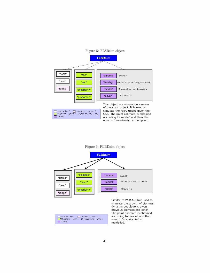
Figure 5: FLSRsim object

Figure 6: FLBDsim object

41

Figure 7: FLIndex object

Figure 8: FLStock object

42