Embed Size (px)
Citation preview

ww.sciencedirect.com
i n t e rn a t i o n a l j o u r n a l o f h y d r o g e n en e r g y 4 1 ( 2 0 1 6 ) 1 7 5 2 6e1 7 5 3 8
Available online at w
ScienceDirect
journal homepage: www.elsevier .com/locate/he
Flatness-based feedforward control of polymerelectrolyte membrane fuel cell gas conditioningsystem
J�anos Kancs�ar*, Martin Kozek, Stefan Jakubek
Institute of Mechanics and Mechatronics, Division of Control and Process Automation, Vienna University of
Technology, Austria
a r t i c l e i n f o
Article history:
Received 17 March 2016
Received in revised form
27 May 2016
Accepted 7 June 2016
Available online 25 July 2016
Keywords:
PEM fuel cell testbed
Nonlinear control
Exact linearisation
Differential flatness
* Corresponding author. Tel.: þ43 1 58801 32E-mail address: [email protected]
http://dx.doi.org/10.1016/j.ijhydene.2016.06.00360-3199/© 2016 Published by Elsevier Ltd o
a b s t r a c t
Manufacturers of automotive applications rely on high-performance testing environments
for the development of polymer electrolyte membrane fuel cell (PEMFC) technologies. The
main component of a PEMFC testbed is the gas conditioning system, which controls the
inlet gas temperature, stack pressure, relative humidity and mass flow of the gas at the
inlet of the PEMFC stack. This paper presents a control concept for a highly dynamic PEMFC
gas conditioning system. The main control challenge lies in the decoupling of the gov-
erning thermodynamic quantities. Therefore, the nonlinear control concept of exact input
eoutput linearisation with an extended PID control structure is applied. Constraints on the
actuators are incorporated by formulating the resulting control law as an optimisation
problem. The robustness with respect to parameter uncertainties for the model is shown
by investigating the trajectory tracking error of the disturbed system. Simulation results
show an overall good performance for the trajectory tracking and demonstrate the
robustness of the model against parameter uncertainties.
© 2016 Published by Elsevier Ltd on behalf of Hydrogen Energy Publications LLC.
Introduction
Due to increasing emission standards [1], automotive manu-
facturers are looking for ways to reduce pollution or even
replace internal combustion engines by alternative propulsion
systems. One of the most promising technologies are polymer
electrolyte membrane fuel cell (PEMFC) powered vehicles.
Compared to other fuel cell technologies, PEMFCs have the
advantages of operating at low temperature, fast response,
high power density and zero emission.
By utilising the electrochemical reaction of hydrogen and
oxygen to create energy, the emission of air pollutants is
decreased to zero. In order to develop and increase the effi-
ciency of PEMFC systems, manufacturers rely on a high
5518..at (J. Kancs�ar).86n behalf of Hydrogen En
performance testing environment on component level. A
schematic view of a fuel cell system is given in Fig. 1. The gas
conditioning system in a PEMFC system is one of the main
components, and it is responsible for conditioning the inlet
gas for the PEMFC stack.
There are four main control tasks for a PEMFC gas condi-
tioning system. These deduce from the main challenges to
reduce the rate of degradation of the PEMFCmembrane under
load changes [2].
First, the control of the inlet gas mass flow rate. This pro-
vides the gas supply for the fuel cell and prevents the system
from lack of reactants and, therefore, prevents the stack from
so called starvation, which would otherwise increase the
degradation of the stack [3,4].
ergy Publications LLC.
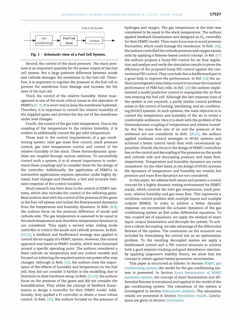
Gasconditioning
Fuel CellStack
Exhaust
Fuel Cell System
Fig. 1 e Schematic view of a Fuel Cell System.
i n t e r n a t i o n a l j o u r n a l o f h y d r o g e n en e r g y 4 1 ( 2 0 1 6 ) 1 7 5 2 6e1 7 5 3 8 17527
Second, the control of the stack pressure. The stack pres-
sure is an important quantity for the power output of the fuel
cell system. But a large pressure difference between anode
and cathode damages the membrane in the fuel cell. There-
fore, it is important to regulate the pressure in the fuel cell to
prevent the membrane from damage and increase the life
time of the fuel cell.
Third, the control of the relative humidity. Water man-
agement is one of the most critical issues in the operation of
PEMFCs [5e7]. It is most vital to keep themembrane hydrated.
Therefore, it is important to control the relative humidity of
the supplied gases and prevent the dry out of the membrane
under load changes.
Fourth, the control of the gas inlet temperature. Due to the
coupling of the temperature to the relative humidity, it is
evident to additionally control the gas inlet temperature.
These lead to the control requirements of a gas condi-
tioning system: inlet gas mass flow control, stack pressure
control, gas inlet temperature control and control of the
relative humidity of the stack. These thermodynamic quan-
tities are coupled through various relations. To successfully
control such a system, it is of utmost importance to under-
stand these couplings and to consider them for the design of
the controller. Additionally, the application of PEMFCs in
automotive applications requires operation under highly dy-
namic load changes and therefore, a fast and accurate tran-
sient response of the control variables.
Much research has been done in the control of PEMFC sys-
tems, which also includes the control of the inflowing gases.
Most authors deal with the control of the pressure of the gases
in the fuel cell system and isolate the flow/pressure dynamics
from the temperature and humidity dynamics. In Refs. [8,9],
the authors focus on the pressure difference of anode and
cathode side. The gas temperature is assumed to be equal to
thestack temperatureand, therefore, temperaturedynamics is
not considered. They apply a second order sliding mode
controller to control the anode and cathode pressure. In Refs.
[10,11], a feedback and feedforward strategy was applied to
control the air supply of a PEMFC system.However, the control
approach was based on PEMFCmodels, which were linearised
around a specific operating point. The authors considered a
fixed cathode air temperature and one control variable and
focused on achieving the required systemnet power after step
changes. Although in Refs. [12], the authors state the impor-
tance of the effects of humidity and temperature on the fuel
cell, they did not consider it further in the modelling, due to
limitation in their hardware setup. In Refs. [13,14], the authors
focus on the pressure of the gases and did not consider the
humidification. They utilise the concept of feedback linear-
isation to design a controller for their PEMFC model. Addi-
tionally, they applied a PI controller to obtain a more robust
control. In Refs. [15], the authors focused on the pressure of
hydrogen and oxygen. The gas temperature at the inlet was
considered to be equal to the stack temperature. The authors
applied feedback linearisation and designed an H∞ controller
for their PEMFCmodel. Theirmain focuswas to avoid pressure
fluctuation, which could damage the membrane. In Refs. [16],
theauthors controlled thecathodepressureandoxygenexcess
ratio by applying a flatness-based control concept. In Ref. [17]
the authors propose a fuzzy-PID control for air flow regula-
tion and analyse and verify the simulation results to prove the
efficiency of the proposed fuzzy-PID control against the con-
ventional PID control. They conclude that a feedforward part is
a great help to improve the performance. In Ref. [18] the au-
thors investigateda timedelaycontrol to increase the transient
performance of PEM fuel cells. In Ref. [19] the authors imple-
mented a model predictive control to manipulate the air flow
rate entering the fuel cell. Although the fast response time of
the system is not required, a partly similar control problem
arises in the control of heating, ventilating, and air condition-
ing (HVAC) systems. In such systems, the main objective is to
control the temperature and humidity of the air to create a
comfortable ambience. Here it is dealt with the problem of the
thermodynamic coupling of temperature and relative humid-
ity. But the mass flow rate of air and the pressure of the
ambience are not considered. In Refs. [20,21], the authors
applied nonlinear control strategies to HVAC systems and
achieved a better control result than with conventional ap-
proaches. Overall, the focus in the design of PEMFC controllers
lies on the control and decoupling of the pressure on the anode
and cathode side and decoupling pressure and mass flow,
respectively. Temperature and humidity dynamics are rarely
considered. On the other hand, in the design of HVAC systems
the dynamics of temperature and humidity are treated, but
pressure andmass flow dynamics are not considered.
In this paper, we address both issues and present a control
concept for a highly dynamic testing environment for PEMFC
stacks, which controls the inlet gas temperature, stack pres-
sure, relative humidity and gas mass flow. This represents a
nonlinear control problem with multiple inputs and multiple
outputs (MIMO). In order to achieve a better dynamic
response, we incorporate the actuator dynamics of the gas
conditioning system as first order differential equations. To
this coupled set of equations, we apply the method of exact
inputeoutput linearisation and decouple the system. To ach-
ieve a robust decoupling, we take advantage of the differential
flatness of the system. The constraints on the actuators are
included by formulating the control law as an optimisation
problem. To the resulting decoupled system we apply a
feedforward control and a PID control structure to achieve
both a good setpoint tracking and good disturbance rejection.
By applying Lyapunov's stability theory, we show that the
concept is robust against tested parameter uncertainties.
This paper is structured as follows: In Section PEMFC gas
conditioning system, the model for the gas conditioning sys-
tem is presented. In Section Exact linearisation of MIMO
nonlinear system, the concept of exact linearisation and dif-
ferential flatness is introduced and applied to themodel of the
gas conditioning system. The robustness of the system is
investigated in Section Robustness analysis. The simulation
results are presented in Section Simulation results. Conclu-
sions are given in Section Conclusion.

Table 1 e Operating ranges of actuators and outputvariables.
Actuator Range Output Range
uG 4�40 kgh�1 T 20�100 �C_Q 0�9 kW p 1.1�3 bar
uS 0�30 kgh�1 4 0�100%
uNozzle 0�2 cm2 _mout 0�70 kgh�1
i n t e rn a t i o n a l j o u r n a l o f h y d r o g e n en e r g y 4 1 ( 2 0 1 6 ) 1 7 5 2 6e1 7 5 3 817528
PEMFC gas conditioning system
In the following, we present the hardware concept for a gas
conditioning system for a PEMFC testbed and derive the
mathematical model, which describes the system. For the
reason of readability, first, we introduce the subscripts G for
gas and S for steam and second, we use the operator ddt to
indicate a time derivative and the dot operator to indicate a
mass flow. In the following sections we only use the dot
operator because the mass flow is part of the state vector and
we do not need to distinguish between time derivatives and
mass flows.
Hardware setup for the gas conditioning system
As depicted in Fig. 1, the gas conditioning system for the
PEMFC stack takes in gas and provides a controlled environ-
ment for the fuel cell stack. It accomplishes this by controlling
the inlet gas temperature, stack pressure, relative humidity
and gas mass flow to the stack.
In Fig. 2, a schematic of a gas conditioning system for the
cathode channel of a PEMFC is shown. Pressurised gas and
steam are provided at the testbench. The mass flow of both
paths is controlled with a mass flow controller (MFC). The air
path has an additional heater, while the steam path has a
fixed temperature. Both gases are fed into a mixing chamber,
which provides the gas mixture at the outlet. The fuel cell (FC)
stack cathode is depicted after the mixing chamber. At the
outlet of the fuel cell stack cathode, a backpressure valve is
located. The control variables for this setup are the two gas
mass flows controlled by the mass flow controllers, the power
of the heater and the opening area of the backpressure valve.
The outputs to be controlled are located behind the mixing
chamber. These are the inlet gas temperature, stack pressure,
relative humidity and gas mass flow into the fuel cell stack
cathode inlet. A summery and the corresponding operating
ranges are given in Table 1. The operating ranges are calcu-
lated based on a 10 kW PEMFC stack.
Gas dynamics of gas conditioning system model
The mass balance equations in the mixing chamber are given
by Eq. (1). The first equation represents the mass balance for
air. The second equation represents the mass balance for the
steam in the system. The first terms in the equations are the
Fig. 2 e Block diagram of testb
mass flows into the mixing chamber, and the second terms
are the outflowing gases.
ddtmG ¼ _mG; in � _mG; out
ddtmS ¼ _mS; in � _mS; out
(1)
The outflowing mass streams in Eq. (1) are given by
_mG; out ¼ mG
m_mout; _mS; out ¼ mS
m_mout (2)
with
m ¼ mG þmS: (3)
The outflowingmass streams of gas and steamare given by
the mass fractions of the total mass m in the system.
The energy balance of the system is given by Eq. (4).
dUdt
¼ _mG;inhG;in þ _mS;inhS;in � _mouthout; (4a)
dUdt
¼ ddt
mGuG þmSuSð Þ (4b)
where hG,in, hS,in and hout are the specific enthalpies of the
gases and are given by Eq. (6) and uG and uS represent the
specific internal energy of the gases.
With Eq. (2) the last term in Eq. (4a) can be written as
_mouthout ¼ 1m
_moutðmGhG; out þmShS; outÞ: (5)
The specific enthalpies of the gases are defined as
hG; in ¼ cp;GTG;in ; hS; in ¼ cp;STS;in þ r0; (6a)
hG; out ¼ cp;GT ; hS; out ¼ cp;STþ r0 (6b)
where T represents the temperature in the mixing chamber,
TG, in and TS, in are the temperatures of the inflowing gases, cp,Gand cp,S are the specific heat capacities, which are assumed to
ench for cathode channel.

i n t e r n a t i o n a l j o u r n a l o f h y d r o g e n en e r g y 4 1 ( 2 0 1 6 ) 1 7 5 2 6e1 7 5 3 8 17529
be constant over the whole operating range, and r0 is the
latent heat of steam.
To obtain an expression for the specific internal energy, we
insert Eq. (7) into Eq. (6) and obtain the equations given by Eq.
(8).
R ¼ cp � cv; h ¼ uþ pv; RT ¼ pv (7)
where R represents the gas constant, cv the specific heat ca-
pacity and v the specific volume.
uG ¼ cv;GT; uS ¼ cv;STþ r0 (8)
By inserting Eq. (6) and Eq. (8) into Eq. (4) and applying the
time derivative we obtain the equation
ddt
T ¼ 1mGcv;G þmScv;S
$
�_mG; incp;GTG; in þ _mS; in
�cp;STS; in þ r0
�� 1m
_mout
�mGcp;GTþmS
�cp;STþ r0
��� ddtmGcv;GT
� ddtmS
�cv;STþ r0
��; (9)
which describes the temperature dynamics of our system.
The pressure p at the inlet of the fuel cell stack is calculated
by using the ideal gas law given in Eq. (10), with RG and RS
being the gas constants of gas and steam. The volume V of the
system enters through this equation. It has an effect on the
pressure dynamics of the system and is treated as a param-
eter. The volumenot only represents the volume of themixing
chamber but also the volume of the other piping, which have
an effect on the dynamics.
pV ¼ ðmGRG þmSRSÞ T (10)
These equations describe the thermodynamics of the sys-
tem. One important quantity in these equations is the out-
flowing mass stream _mout, which is highly dependent on the
backpressure valve. The relative humidity 4 is given by Eq.
(11).
4 ¼ XRGRS
þ X$
p
psW
�T�; X ¼ mS
mG(11)
where X represents the vapour content in the gas, and psWðTÞ is
the saturation partial pressure given by Magnus' formula in
Eq. (12).
psW
�T� ¼ pm$e
C1$T
C2þT (12)
The parameters pm, C1 and C2 for Eq. (12) are taken fromRef.
[22].
Pressure valve
To model the mass flow through the backpressure valve, the
nonlinear flow equation [23] given in Eq. (13) has been used.
_mout ¼ Ap
ffiffiffiffiffiffi2
RT
r$j
j ¼ffiffiffiffiffiffiffiffiffiffiffiffiffiffiffiffiffiffiffiffiffiffiffiffiffiffiffiffiffiffiffiffiffiffiffiffiffiffiffiffiffiffiffiffiffiffiffiffiffiffiffiffiffik
k� 1
"�p0
p
�2k
��p0
p
�kþ1k
#vuut ; k ¼ cpcv
(13)
The critical pressure is given by
p0
p¼�
2kþ 1
� kk�1
(14)
and the critical flow is given by
jmax ¼�
2kþ 1
� 1k�1
ffiffiffiffiffiffiffiffiffiffiffik
kþ 1
r: (15)
In this equation, A represents the opening area of the
aperture, R the gas constant and p0 the ambient pressure. For
this equation, we have to take into account that the content of
water vapour in the gas mixture changes over the operation
range. Therefore, the gas constant R and the specific heat
capacities cp and cv of the current gas mixture have to be used.
Actuator dynamics of gas conditioning system model
In order to account for the dynamics, which is introduced by
the actuators, we incorporate these into the model. There are
different approaches how this can be achieved. In our
approach, we model the dynamics as first order lag elements
with time constants t1�4. This leads to additional four differ-
ential equations given by Eq. (16).
ddt
_mG; in ¼ 1t1
�uG � _mG; in
�(16a)
ddtTG; in ¼ 1
t2
1cp;G _mG; in
_Q
_mG; in� cp;G
�TG; in � TG; 0
�!(16b)
ddt
_mS; in ¼ 1t3
�uS � _mS; in
�(16c)
d
dt_ANozzle ¼ 1
t4ðuNozzle � ðANozzle � A0ÞÞ (16d)
Eq. (16a) represents the first order lag element for the gas
supply. Eq. (16b) derives from a first order lag element for the
energy balance of the heater depicted in Fig. 2 and the
assumption that ddt
_mG; in ¼ 0 during the heat transfer in the
heater.This implies thatall theenergyprovidedby theheater is
absorbed by increasing the temperature of the current mass
flow, but the mass flow itself is not affected by the process.
Additionally, a temperature offset TG, 0 has been included. This
accounts for the fact that the gas flow can not be cooled below
the initial gas temperature provided at the testbed. Eq. (16c)
represents the first order lag element for steam supply. Eq.
(16d) represents thefirstorder lagelement for thebackpressure
valve with an offset value A0 for the opening area of the valve.
Coupling of the system
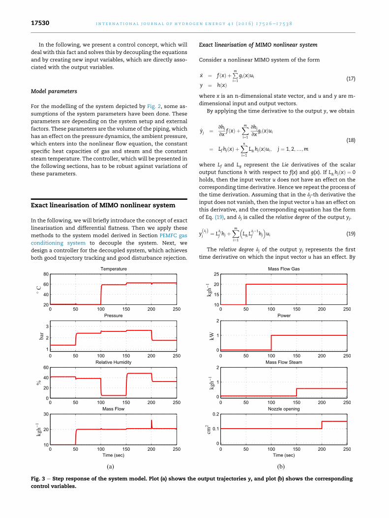
The equations presented in this section are coupled through
various relations. This leads to the fact that the input variables
can not be associated with the output variables. By changing
one input variable, all the output variables are affected in one
or another way. This is illustrated in Fig. 3. The figure shows
the system response for step changes of the input variables.
All the system outputs are affected by each change of the
input variables.
i n t e rn a t i o n a l j o u r n a l o f h y d r o g e n en e r g y 4 1 ( 2 0 1 6 ) 1 7 5 2 6e1 7 5 3 817530
In the following, we present a control concept, which will
deal with this fact and solves this by decoupling the equations
and by creating new input variables, which are directly asso-
ciated with the output variables.
Model parameters
For the modelling of the system depicted by Fig. 2, some as-
sumptions of the system parameters have been done. These
parameters are depending on the system setup and external
factors. These parameters are the volume of the piping, which
has an effect on the pressure dynamics, the ambient pressure,
which enters into the nonlinear flow equation, the constant
specific heat capacities of gas and steam and the constant
steam temperature. The controller, which will be presented in
the following sections, has to be robust against variations of
these parameters.
Exact linearisation of MIMO nonlinear system
In the following, we will briefly introduce the concept of exact
linearisation and differential flatness. Then we apply these
methods to the system model derived in Section PEMFC gas
conditioning system to decouple the system. Next, we
design a controller for the decoupled system, which achieves
both good trajectory tracking and good disturbance rejection.
Fig. 3 e Step response of the system model. Plot (a) shows the
control variables.
Exact linearisation of MIMO nonlinear system
Consider a nonlinear MIMO system of the form
_x ¼ f xð Þ þPmi¼1
gi xð Þui
y ¼ h xð Þ(17)
where x is an n-dimensional state vector, and u and y are m-
dimensional input and output vectors.
By applying the time derivative to the output y, we obtain
_yj ¼ vhj
vxf xð Þ þ
Xmi¼1
vhj
vxgi xð Þui
¼ Lfhj xð Þ þXni¼1
Lgi hj xð Þui; j ¼ 1; 2;…;m
(18)
where Lf and Lg represent the Lie derivatives of the scalar
output functions h with respect to f(x) and g(x). If Lgi hjðxÞ ¼ 0
holds, then the input vector u does not have an effect on the
corresponding time derivative. Hencewe repeat the process of
the time derivation. Assuming that in the dj-th derivative the
input does not vanish, then the input vector u has an effect on
this derivative, and the corresponding equation has the form
of Eq. (19), and dj is called the relative degree of the output yj.
yðdjÞj ¼ L
dj
f hj þXmi¼1
�Lgi L
dj�1
f hj
�ui (19)
The relative degree dj of the output yj represents the first
time derivative on which the input vector u has an effect. By
output trajectories y, and plot (b) shows the corresponding

i n t e r n a t i o n a l j o u r n a l o f h y d r o g e n en e r g y 4 1 ( 2 0 1 6 ) 1 7 5 2 6e1 7 5 3 8 17531
applying this to each output yj, we obtain m equations, which
can be written as
2664yðd1Þ1
yðd2Þ2
«yðdmÞm
3775 ¼
26664Ld1f h1ðxÞLd2f h2ðxÞ
«Ldmf hmðxÞ
37775|fflfflfflfflfflfflfflfflfflffl{zfflfflfflfflfflfflfflfflfflffl}
lðxÞ
þJðxÞ
2664u1
u2
«um
3775 (20)
where the (m � m) matrix J(x) is called the decoupling matrix
and is defined as
JðxÞ ¼
26664Lg1L
d1�1f h1ðxÞ … LgmL
d1�1f h1ðxÞ
Lg1Ld2�1f h2ðxÞ … LgmL
d2�1f h2ðxÞ
« «Lg1L
dm�1f hmðxÞ … LgmL
dm�1f hmðxÞ
37775: (21)
By choosing the control law of the form
u ¼ aðxÞ þ bðxÞ n (22)
with
a xð Þ ¼ �J�1 xð Þ l xð Þ;b xð Þ ¼ J�1 xð Þ (23)
one obtains the new synthetic input vector n
v ¼24 v1
«vm
35 ¼24 yðd1Þ
1
«yðdmÞm
35: (24)
From Eq. (24) it is evident that the inputeoutput relation of
this system is decoupled and can be represented as a chain of
integrators.
IfPm
j¼1dj ¼ dimðxÞ ¼ n, the system has so called full relative
degree and can be transformed into the nonlinear controllable
canonical form [24]. The transformation is given by Eq. (25). It
utilises the Lie derivatives introduced in Eq. (19). The variable z
represents the new state of the transformed system.
z ¼
26666664z1z2«zd1«zn
37777775 ¼ TðxÞ ¼
26666664
h1ðxÞLfh1ðxÞ
«Ld1�1f h1ðxÞ
«Ldm�1f hmðxÞ
37777775 (25)
For systems, which do not have full relative degree, one has
to account for the internal dynamics of the system. More on
how to deal with internal dynamics can be found in Refs. [25]
and [26].
The transformation given by Eq. (25) results in the new
state space representation, given in Eq. (26), where v repre-
sents the new input vector. For this system, linear control
methods can be applied.
_z ¼ Ac zþ Bc v (26)
The matrices Ac and Bc are given by Eq. (27).
Ac ¼
2664Ac;1 0 … 00 Ac;2 … 0« « «0 0 … Ac;m
3775; (27a)
Bc ¼
2664Bc;1 0 … 00 Bc;2 … 0« « «0 0 … Bc;m
3775 (27b)
where the matrix Ac,j is a (dj � dj) matrix, and Bc,j is a (dj � 1)
vector given by Eq. (28).
Ac;j ¼
2666640 1 0 … 00 0 1 … 0« « « «0 0 0 … 10 0 0 … 0
377775; Bc;j ¼
26666400«01
377775 (28)
Differential flatness
Differential flatness is a property of a class of multivariable
nonlinear systems and has first been introduced in Refs. [27]
and [28]. A nonlinear system of the form
_x ¼ fðx;uÞ; xð0Þ ¼ x0 (29)
is said to be differentially flat, if there exists a set of differ-
entially independent variables y ¼ (y1,…,ym) such that the
state variables x and input variables u are functions of these
flat outputs and a finite number of their derivatives.
y ¼ FðxÞ (30a)
x ¼ F�y; _y;…yn�1
�(30b)
u ¼ Jðy; _y;…ynÞ (30c)
In that case, y represents the flat outputs of the system, and
the system is called differential flat or flat system. The Equation
(30) yield that for every given trajectory y, the evolution of the
state variables x and input variables u can be calculated
without the need to integrate the differential equations.
Exact linearisation of gas conditioning system model
From the equations derived in Section PEMFC gas conditioning
system, we formulate the state vector x, the input vector u and
output vector y as follows
x ¼
2666666664
mG
mS
T_mG; in
TG; in
_mS; in
ANozzle
3777777775; u ¼
2664uG_Q
uS
uNozzle
3775; y ¼
2664Tp4_mout
3775 (31)
With this representation, we obtain an equation of the
form of Eq. (17). We apply the Lie derivatives to the output y
and obtain that the first three outputs y1�3 have a relative de-
gree of two (d1 ¼ d2 ¼ d3 ¼ 2), and the last output y4 has a relative
degree of one (d4 ¼ 1). Due to the complex couplings in the
output functions, the relative degree of two of these outputs
and the dimension of the state vector x, the calculations get

i n t e rn a t i o n a l j o u r n a l o f h y d r o g e n en e r g y 4 1 ( 2 0 1 6 ) 1 7 5 2 6e1 7 5 3 817532
large and are not insightful. For the reason of readability, we
do not give the detailed calculations of the Lie derivatives.
Since the systemhas full relative degree, we can transform it
using the nonlinear transformation introduced in Eq. (25). For
our system the transformation takes the form of Eq. (32).
z ¼ TðxÞ ¼
2666666664
h1ðxÞLfh1ðxÞh2ðxÞLfh2ðxÞh3ðxÞLfh3ðxÞh4ðxÞ
3777777775¼
2666666664
y1
_y1
y2
_y2
y3
_y3
y4
3777777775(32)
where, in accordance to Eq. (19), the Lie derivatives for the
outputs (i ¼ 1,2,3), which have relative degree of two (di ¼ 2),
yield LfhiðxÞ ¼ _yi. From this transformationwe obtain a system
of the form
_z ¼ Ac zþ Bc b xð Þ�1 u� a xð Þð Þu ¼ a xð Þ þ b xð Þ n (33)
where Ac and Bc are the matrices in controllable canonical
form, and n is the new input variable.
InFig. 4, thenonlinear transformationof the coupled system
given by Eq. (17) into the decoupled system given by Eq. (33) is
depicted. Fig. 4b represents a schematic view of the decoupled
systemasachainof integrators for eachchannel. The inputs for
the decoupled system are the new input variables n, which are
integrated to obtain the output y. The length of the chain of
integrators is equal to the relative degree dj of the output yj.
For the decoupling of the system, the knowledge of the
state vector x is required, which corresponds to the current
operation point of the system. If the states can bemeasured or
observed, they can be fed back into the decoupling matrix. In
that case one has to take care of possible feedback distur-
bances from the system.
Flatness based calculation of the state vector
The system outputs y1�4 are flat outputs of the system. This
can be utilised to minimise the feedback disturbance on the
decoupling of the system. Therefore, we apply a flatness-
based feedforward calculation of the states x. Instead of
Fig. 4 e Schematic view of the transformation of the coupled syst
is represented as chain of integrators with the new input varia
relative degree dj of the output yj.
using a state vector feedback for the decoupling, we apply the
so calculated states xFF in Eq. (33).
The states xFF are calculated offline by solving the set of
equations given by Eq. (32). This leads to the functional de-
pendency given in Eq. (30). The so obtained states are then fed
into the system.
Trajectory tracking and error dynamics
To achieve both, a good trajectory tracking and good distur-
bance rejection, we design a Two-Degree-of-Freedom (2DoF)
controller for the decoupled system.
We want the output y(t) to track a reference signal ydmd(t).
For the decoupled system, the new input variable nj represents
the input to dj chain of integrators. Therefore, the feedforward
signal has to be the dj-th derivative of the trajectory to be
followed by the output yj. This can be directly seen in Fig. 4b.
As controller we choose a PID(d�1) control structure, whichwas
introduced in Refs. [29,30]. To design the PID(d�1) control
structure, we define the tracking error ej
ejðtÞ ¼ yjðtÞ � ydmd;jðtÞ; j ¼ 1;…; 4 (34)
and further the tracking error vector ej,k with k ¼ 0,…,dj
ej;0 ¼Z t
0
ejðtÞ dt; ej;1 ¼ ej; ej;2 ¼ _ej (35)
Combining these, we canwrite the new input as sum of the
feedforward part and the PID(d�1) control structure
nj ¼ €ydmd;j � KI;j ej;0 � KP;j ej;1 tð Þ � KD;j ej;2 tð Þ; j ¼ 1; 2;3n4 ¼ _ydmd;4 � KI;j e4;0 � KP;4 e4;1 tð Þ (36)
The error dynamics for the first three outputs (j ¼ 1,2,3),
which have a relative degree of dj ¼ 2, are given by
24 _ej;0_ej;1_ej;2
35 ¼
0BBBBBBB@24 0 1 00 0 10 0 0
35|fflfflfflfflfflfflfflfflffl{zfflfflfflfflfflfflfflfflffl}
Ac;j
�24001
35|fflffl{zfflffl}
Bc;j
KI;j; KP;j; KD;j
�|fflfflfflfflfflfflfflfflfflfflfflfflfflfflfflffl{zfflfflfflfflfflfflfflfflfflfflfflfflfflfflfflffl}
Kj
1CCCCCCCA$
24 ej;0ej;1ej;2
35 (37)
em (a) into the decoupled system (b). The decoupled system
ble n. The length of the chain of integrators is equal to the

i n t e r n a t i o n a l j o u r n a l o f h y d r o g e n en e r g y 4 1 ( 2 0 1 6 ) 1 7 5 2 6e1 7 5 3 8 17533
and the error dynamics for the fourth output, which has a
relative degree of d4 ¼ 1, is given by
�_e4;0_e4;1
¼
0BBBBB@�0 10 0
|fflfflfflfflffl{zfflfflfflfflffl}
Ac;4
��01
|ffl{zffl}Bc;4
½KI;4; KP;4 �|fflfflfflfflfflfflfflfflffl{zfflfflfflfflfflfflfflfflffl}K4
1CCCCCA$
�e4;0e4;1
(38)
Combining these equations we can rewrite it as
_e ¼ ðAc � BcKÞ e (39)
where e is a (11� 1) vector combining Eq. (37), and Eq. (38),Ac is
a (11 � 11) matrix, Bc is a (11 � 4) matrix, and K is a (4 � 11)
matrix. The vectors and matrices are given in Eq. (40). The
asymptotic tracking is achieved by placing the desired poles of
(Ac � BcK) in the left-half plane.
Ac ¼
2664Ac;1 0 0 00 Ac;2 0 00 0 Ac;3 00 0 0 Ac;4
3775; (40a)
Bc ¼
2664Bc;1 0 0 00 Bc;2 0 00 0 Bc;3 00 0 0 Bc;4
3775; (40b)
K ¼
2664K1 0 0 00 K2 0 00 0 K3 00 0 0 K4
3775 (40c)
Fig. 5 shows the structure of the system. S represents the
gas conditioning system,whichwasmodelled by Eq. (1), Eq. (9)
and Eq. (16). The decoupling is done by the S�1 block, which
represents Eq. (22). It uses the flatness-based feedforward
states xFF to accomplish the decoupling. The channels of the
so obtained system are decoupled, and a new input vector n is
introduced. On each channel of this decoupled system, a 2DoF
controller is designed to achieve both good trajectory tracking
and good disturbance rejection.
For the purpose of clarity we decompose Eq. (39) and write
it as
_e ¼ Ac eþ Bc
hbðxÞ�1ðu� aðxÞÞ � yðdÞ
dmd
i(41a)
u ¼ aðxÞ þ bðxÞ n (41b)
Fig. 5 e Block diagram of Two-Degree-of-Freedom (2DoF)
Controller.
n ¼ yðdÞdmd � K e (41c)
In this formulation, the decoupling terms a(x) and b(x)
appear in the control law. To this representation of the error
dynamics we will later refer to discuss the robustness of the
system.
Including constraints on the input variables
During operation the following two problems arise in calcu-
lating the input vector.
First, the decoupling matrix J(x) is not invertible for all
states x. Although this is not the case if the system is in the
operating range described in Table 1, for the startup the sys-
tem has to cross a region, where J(x) does not have full rank. A
physical interpretation of the startup is the following: At
startup the system pressure p is equal to the ambient pressure
p0, and therefore, the backpressure valve has no effect on the
outflowing mass flow _mout. Hence, the decoupling matrix J(x)
does not have full rank. Therefore, we need an additional
condition to invert the decoupling matrix. So we can steer the
system into the operating range, where the decoupling matrix
J(x) has full rank and the additional condition can be dropped.
Second, constraints on the actuators lead to deviations of
the output trajectory. In order to achieve a better trajectory
tracking, we want to minimise these deviations.
Both problems can be solved by introducing the following
Lagrange function
L ¼ a12uTR uþ 1
2
�yðdÞ � yðdÞ
dmd
�TQ�yðdÞ � yðdÞ
dmd
�þ lTðMu� gÞ (42)
where R and Q are (4 � 4) symmetric and positive definite
matrices, which are used as weighting matrices, M is a (4 � 4)
identity matrix, and g is a (4 � 1) vector of the actuator con-
straints listed in Table 1.
The first term is active (a¼ 1) if the decouplingmatrix is not
invertible, otherwise a ¼ 0. This minimises additionally the
input vector u. This additional condition is responsible for the
invertibility of the decouplingmatrix J(x) if it does not have full
rank.
The second term minimises the deviation of the trajectory
curvature. Whereas ðyðdÞ � yðdÞdmdÞ is the equivalent formulation
of Eq. (22) for optimisation.
The third term represents the Lagrange Multiplier l for the
active constraints. If the constraints are reached by one or
more input variables, the constraints are added using the
active-set-method.
By reformulating Eq. (42) into
L ¼ 12uTE uþ 1
2uTFþ lTðMu� gÞ (43)
with
E ¼ Rþ J xð ÞTQ J xð Þ;F ¼ J xð ÞTQ l xð Þ � y dð Þ
dmd
� � (44)
we can write the solution as
lact ¼ � Mact E�1MT
act
� ��1gact þMact E
�1F� �
;
u ¼ �E�1 MTactlact þ F
� �;
(45)

Fig. 6 e System in which the decoupling block S¡1 has a
different parameter set Q than S.
Table 2 e Model parameters used for the simulation.
Parameter Value
Volume 14 137 cm3
cp,G 1.04 kJ kg�1 K�1
cp,S 1.89 kJ kg�1 K�1
TS 141 �Cp0 1 bar
Fig. 7 e Plot (a) shows the achieved output trajectories y (green ful
(b) shows the corresponding control variables. (For interpretatio
is referred to the web version of this article.)
i n t e rn a t i o n a l j o u r n a l o f h y d r o g e n en e r g y 4 1 ( 2 0 1 6 ) 1 7 5 2 6e1 7 5 3 817534
where Mact and lact represent the active constraints. The so
obtained Eq. (45) replaces Eq. (22) in S�1 in Fig. 5.
Robustness analysis
In the following, we present a robustness analysis with
respect to parameter uncertainties for the derived system.We
discuss the robustness of the decoupling of the system in case
of deviations of the system parameters and the parameters
assumed for the calculation of the decoupling.
System parameters
The method of inputeoutput exact linearisation, which has
been applied in Section Exact linearisation of MIMO nonlinear
system, relies on the exact cancelation of a and b in Eq. (41a)
and the control law Eq. (41b). If this is not the case, a
coupling of the output vector y will remain.
To analyse the robustness of the system, we introduce the
parameter vector Q
Q ¼
266664Volume
cp;Gcp;STS
p0
377775 (46)
l line) and the desired trajectories ydmd (blue dashed line). Plot
n of the references to colour in this figure legend, the reader

Fig. 8 e Ratio plots of achieved to desired output
trajectories for parameter variations.
i n t e r n a t i o n a l j o u r n a l o f h y d r o g e n en e r g y 4 1 ( 2 0 1 6 ) 1 7 5 2 6e1 7 5 3 8 17535
which contains the parameters discussed in Section PEMFC
gas conditioning system. These are the volume of the mix-
ing chamber and the piping, the specific heat capacities,
which are assumed to be constant, the steam temperature
and the ambient pressure during operation. These parameters
have an effect on the dynamics of the system equations
derived in Section PEMFC gas conditioning system and enter
as well in the calculation of the decoupling derived in Section
Fig. 9 e Calculated trajectory jjd(e)jj¡kjjejj in accordance to
Lemma 13.3. For the trajectories one finds an e, which
fulfils the Lemma.
Exact linearisation of MIMO nonlinear system. Fig. 6 shows
the case, where the decoupling block S�1Q and the system SQ0
have a different set of parameters. In that case the system is
not fully decoupled.
Disturbed system
To consider the parameter deviations of the system, we
introduce the error of the nominal system Eq. (47a) and the
error of the disturbed system Eq. (47b).
ejðtÞ ¼ yjðt;Q0Þ � ydmd;jðtÞ (47a)
bejðtÞ ¼ yjðt;QÞ � ydmd;jðtÞ (47b)
where Q0 is the unperturbed parameter vector and Q the
perturbed vector. Similar to Eq. (41), the error dynamics of the
disturbed system can be written as
_e ¼ Ac eþ Bc b xð Þ�1 u� a xð Þð Þ � y dð Þdmd
h iu ¼ ba xð Þ þ bb xð Þ nn ¼ y dð Þ
dmd � K e
(48)
where ba and bb arise from the disturbed system S�1Q , and a and
b arise from the undisturbed system SQ0. Combining these
equations, we obtain
_e ¼ ðAc � Bc KÞ eþ Bc dðeÞ (49)
where d(e) represents the perturbation of the nominal system,
and is given by
Fig. 10 e Initialisation with different initial conditions. The
Plot shows the achieved output trajectories y (green full line)
and the desired trajectories ydmd (blue dashed line). (For
interpretation of the references to colour in this figure
legend, the reader is referred to the web version of this
article.)

Table 3 e Mean squared error for different magnitudes of measurement noise. The magnitude is given as standarddeviation of the normal distribution.
Measurement noise Case 1 Case 2 Case 3
s1 0.1 �C 0.5 �C 1 �Cs2 0.002 bar 0.01 bar 0.1 bar
s3 0.2% 1% 5%
s4 0.07 kgh�1 0.1 kgh�1 1 kgh�1
MSE Temperature 1.6$10�3 �C 4$10�3 �C 4.6$10�2 �CMSE Pressure 2.8$10�6 bar 3.8$10�6 bar 6.4$10�5 bar
MSE Relative Humidity 6.4$10�4% 9.5$10�3% 0.3%
MSE Mass Flow 1.3$10�3 kgh�1 1.5$10�3 kgh�1 3.6$10�2 kgh�1
Table 4 e The different initial conditions for the systemoutputs yj, which are used in the simulation.
Output Case 1 Case 2 Case 3
y1 60 �C 10 �C 30 �Cy2 1.5 p0 0.8 p0 1.2 p0y3 5% 21% 0%
y4 3 kgh�1 0 kgh�1 21 kgh�1
i n t e rn a t i o n a l j o u r n a l o f h y d r o g e n en e r g y 4 1 ( 2 0 1 6 ) 1 7 5 2 6e1 7 5 3 817536
dðeÞ ¼ b�1hðba � aÞ þ
�bb � b� �
yðdÞdmd � K e
�þ bb K ðe� beÞi (50)
The perturbation term d(e) arises from the incomplete
decoupling of the system and affects all four decoupled sys-
tems. To study the effect of this perturbation on the system,
we apply the following Lemma taken from Ref. [26].
Lemma 13.3 Consider the closed-Loop system (49), where
(Ac � BcK) is Hurwitz.Let P ¼ PT > 0 be the solution of the Lya-
punov equation
PðA� BKÞ þ ðA� BKÞTP ¼ �I
and k be a nonnegative constant less than 1/(2jjPBjj2).
� If jjd(e)jj�k jjejj for all e, the origin of (49) will be globally
exponentially stable.
� If jjd(e)jj�k jjejjþe for all e, the state e will be globally ulti-
mately bounded by ec for some c>0.
The proof of this Lemma can be found in [26]. For each
trajectory ydmd, we can calculate an upper boundary in
accordance to the Lemma. Simulation results for the param-
eter varied system will be shown in the following section.
Simulation results
In the following, the simulation results for the proposed
nonlinear multivariable control strategy are presented. The
parameters used for the simulation are listed in Table 2.
Results for the decoupled system
The simulations have been performed with setpoint changes
in the operating range defined in Table 1. Whereas the tra-
jectories for the setpoint changes have been calculated in
accordance to the relative degree of the corresponding output.
Fig. 7a shows the comparison of the desired trajectories ydmd
(blue dashed line) and the achieved output trajectories y (green
full line) of the system. The plot shows good agreement for all
trajectories. The poles of the controllers have been placed as
following: For the channels with d ¼ 2, the poles are at s1 ¼ �1,
s2,3 ¼ �8 ± 1j, and for the channel with d ¼ 1, the poles are at
s1,2¼�5. This configuration is robust for awide range of tested
parameter variations. The results for disturbances on the
system are shown in Section Simulation results for
disturbances on the system.
The corresponding control inputs u are shown in Fig. 7b.
The coupling of the system can be seen on the control inputs.
For each alteration of the trajectories shown in Fig. 7a, all
control inputs have to be altered in order to achieve the
decoupling and hence the desired output trajectory y.
The limiting factors for the trajectory slopes are the actu-
ator dynamics, whichwemodelled by first order lag elements.
In order to achieve a fast response of the system, the actuators
have to be able to follow the rapid change of the control input.
Simulation results for disturbances on the system
Fig. 8 shows simulation results for the parameter varied sys-
tem. The plot shows the ratio of achieved to desired output
trajectories for a parameter varied system. For the simulation
the entries of the parameter vector Q have been varied by the
following values: Volume �50%, cp,G þ 50%, cp,S � 50%,
TS þ 50%, p0 þ 50%. Therefore, the system is not fully decou-
pled, and the PID(d�1) controller has to correct the trajectories.
For the simulations the controller configuration introduced in
Section Results for the decoupled system are used, which is
robust for a wide range of tested parameter variations.
The plot shows that small deviations from the desired
trajectory appear, and the controller has to correct the tra-
jectories. The largest deviation is around 1 � 2%, which is
sufficiently small. The simulations also show that the
flatness-based feedforward calculation of the states x stabil-
ises the decoupling of the system, and no feedback distur-
bances affect the decoupling matrix.
Additionally, we investigate the stability of the system for
parameter uncertainties as introduced in Section Robustness
analysis. Therefore, we calculate the error d(e) in Eq. (49). Fig
9 shows the calculated value of jjd(e)jj�k jjejj in accordance to
the Lemmapresented in Section Robustness analysis. The plot
illustrates that for the trajectories yj we can find an ε, which
fulfils the Lemma stated in Section Robustness analysis.
i n t e r n a t i o n a l j o u r n a l o f h y d r o g e n en e r g y 4 1 ( 2 0 1 6 ) 1 7 5 2 6e1 7 5 3 8 17537
Therefore, we conclude that the system along this trajectories
is robust against this perturbation of parameters.
The effect of the initial conditions on the system are
investigated by choosing different initial conditions and test
for the convergence of the system. In Fig. 10 three different
initial conditions for the system outputs yj are chosen. The
values for the system outputs are given in Table 4. Due to the
flatness of the system the state vector x0 can be calculated
from the system outputs. The simulation shows that for all
three initial conditions the trajectories yj converge to the
desired trajectories ydmd.
The effect of measurement noise on the performance of
the controller is investigated by applying a normal distributed
noise on the output variables yj. The standard deviations for
the noise are given in Table 3. The deviation is evaluated as
the mean squared error of the output variables yj and the
trajectories ydmd. Due to the feedforward part of the controller
the noise does not affect the decoupling and the controller
shows stable performance for the investigated noise levels.
Conclusion
In this paper we present a control concept for a highly dy-
namic testing environment for PEMFC stacks, which controls
the inlet gas temperature, stack pressure, relative humidity
and gas mass flow.
Based on a presented hardware concept, we derive a sys-
tem model, which presents a nonlinear control problem with
multiple inputs and multiple outputs. In order to achieve a
better dynamic response of the system, we incorporate the
actuator dynamics of the gas conditioning system as first
order lag elements.
To this coupled set of equations we apply the method of
exact inputeoutput linearisation and decouple the system. In
order to achieve a robust decoupling, we take advantage of the
differential flatness of the system. The constraints on the
actuators are included by formulating the control law as an
optimisation problem. For the resulting decoupled system, we
design a 2DoF controller with a feedforward part and a PID like
control structure. The performed simulations show that the
presented decoupling of the system and the designed
controller are able to achieve a good trajectory tracking.
The robustness of the system against parameter un-
certainties is tested by considering the error of the decoupling
as perturbation of the nominal system. To this disturbed
system, we apply Lyapunov's stability theory and show that
the concept is robust for the tested parameter uncertainties.
Additionally, we investigate the presented control concept
for the effect of different initial conditions of the system and
the impact of measurement noise on the system.
Acknowledgement
This work was supported by the Austrian Research Promotion
Agency (FFG, No. 840395) in cooperation with AVL List GmbH
and the Hydrogen Center Austria (HyCentA).
r e f e r e n c e s
[1] European Parliament, Regulation (eu) no 333/2014 of theeuropean parliament and of the council of 11 march 2014amending regulation (ec) no 443/2009 to define themodalities for reaching the 2020 target to reduce CO2
emissions from new passenger cars, Off J European Union(Downloaded 18/11/2015).
[2] Zhang J, Zhang H, Wu J, ZhangJiujun. PEM fuel cell testingand diagnosis. Amsterdam: Elsevier; 2013. http://dx.doi.org/10.1016/B978-0-444-53688-4.00008-5.
[3] Taniguchi A, Akita T, Yasuda K, Miyazaki Y. Analysis ofelectrocatalyst degradation in PEMFC caused by cellreversal during fuel starvation. J Power Sources2004;130(1):42e9.
[4] Taniguchi A, Akita T, Yasuda K, Miyazaki Y. Analysis ofdegradation in PEMFC caused by cell reversal during airstarvation. Int J Hydrogen Energy 2008;33(9):2323e9.
[5] Yousfi-Steiner N, Mocot�eguy P, Candusso D, Hissel D,Hernandez A, Aslanides A. A review on PEM voltagedegradation associated with water management: impacts,influent factors and characterization. J Power Sources2008;183(1):260e74. http://dx.doi.org/10.1016/j.jpowsour.2008.04.037.
[6] Damour C, Benne M, Grondin-Perez B, Chabriat J-P, Pollet BG.A novel non-linear model-based control strategy to improvePEMFC water management the flatness-based approach. Int JHydrogen Energy 2015;40(5):2371e6. http://dx.doi.org/10.1016/j.ijhydene.2014.12.052.
[7] Haddad A, Bouyekhf R, El Moudni A. Dynamic modeling andwater management in proton exchange membrane fuel cell.Int J Hydrogen Energy 2008;33(21):6239e52. http://dx.doi.org/10.1016/j.ijhydene.2008.06.014.
[8] Matraji I, Laghrouche S, Wack M. Pressure control in a PEMfuel cell via second order sliding mode. Int J Hydrogen Energy2012;37(21):16104e16. advances in Hydrogen Production(Selected papers from ICH2P-2011), http://dx.doi.org/10.1016/j.ijhydene.2012.08.007.
[9] Matraji I, Ahmed FS, Laghrouche S, Wack M. Comparison ofrobust and adaptive second order sliding mode control inPEMFC air-feed systems. Int J Hydrogen Energy2015;40(30):9491e504. http://dx.doi.org/10.1016/j.ijhydene.2015.05.090.
[10] Pukrushpan J, Stefanopoulou A, Peng H. Modeling andcontrol for PEM fuel cell stack system. In: American ControlConference, 2002. Proceedings of the 2002, vol. 4; 2002.p. 3117e22. http://dx.doi.org/10.1109/ACC.2002.1025268.
[11] Pukrushpan J, Peng H, Stefanopoulou AG. Control-orientedmodeling and analysis for automotive fuel cell systems. JDyn Syst Meas Control 2004;126(1):14e25.
[12] Rodatz P, Paganelli G, Guzzella L. Optimizing air supplycontrol of a PEM fuel cell system. In: American ControlConference, 2003. Proceedings of the 2003, vol. 3. IEEE; 2003.p. 2043e8.
[13] Na W, Gou B, Diong B. Nonlinear control of PEM fuel cells byexact linearization. In: Industry Applications Conference,2005. Fourtieth IAS Annual Meeting. Conference Record ofthe 2005, Vol. 4; 2005. p. 2937e43. http://dx.doi.org/10.1109/IAS.2005.1518877.
[14] NaW, Gou B. Feedback-linearization-based nonlinear controlfor PEM fuel cells. IEEE Trans Energy Convers2008;23(1):179e90.
[15] Li Q, Chen W, Wang Y, Jia J, Han M. Nonlinear robust controlof proton exchange membrane fuel cell by state feedbackexact linearization. J Power Sources 2009;194(1):338e48. XIthPolish Conference on Fast Ionic Conductors 2008, http://dx.doi.org/10.1016/j.jpowsour.2009.04.077.

i n t e rn a t i o n a l j o u r n a l o f h y d r o g e n en e r g y 4 1 ( 2 0 1 6 ) 1 7 5 2 6e1 7 5 3 817538
[16] Danzer MA, Wilhelm J, Aschemann H, Hofer EP. Model-based control of cathode pressure and oxygen excess ratioof a PEM fuel cell system. J Power Sources2008;176(2):515e22.
[17] Ou K, Wang Y-X, Li Z-Z, Shen Y-D, Xuan D-J. Feedforwardfuzzy-PID control for air flow regulation of PEM fuel cellsystem. Int J Hydrogen Energy 2015;40(35):11686e95.
[18] Kim Y, Kang S. Time delay control for fuel cells withbidirectional DC/DC converter and battery. Int J HydrogenEnergy 2010;35(16):8792e803. http://dx.doi.org/10.1016/j.ijhydene.2010.05.022.
[19] Gruber J, Doll M, Bordons C. Design and experimentalvalidation of a constrained MPC for the air feed of a fuel cell.Control Eng Pract 2009;17(8):874e85. http://dx.doi.org/10.1016/j.conengprac.2009.02.006.
[20] Rehrl J, Horn M. Temperature control for HVAC systemsbased on exact linearization and model predictive control.In: Control Applications (CCA), 2011 IEEE InternationalConference on. IEEE; 2011. p. 1119e24.
[21] Thosar A, Patra A, Bhattacharyya S. Feedback linearizationbased control of a variable air volume air conditioningsystem for cooling applications. ISA Trans 2008;47(3):339e49.
[22] Plant RS, Yano J-I. Parameterization of atmosphericconvection, vol. 1. Imperial College Press; 2015.
[23] Elger D, Williams B, Crowe C, Roberson J. Engineering fluidmechanics, vol. 10. Wiley; 2012.
[24] Isidori A. Nonlinear control systems. 3rd ed. Secaucus, NJ,USA: Springer-Verlag New York, Inc.; 1995.
[25] Slotine J-J, Li W. Applied nonlinear control. Prentice Hall;1991.
[26] Khalil HK. Nonlinear systems, vol. 3. Prentice Hall; 2002.[27] Fliess M, L�evine J, Martin P, Rouchon P. Flatness and defect of
non-linear systems: introductory theory and examples. Int JControl 1995;61(6):1327e61. http://dx.doi.org/10.1080/00207179508921959. http://dx.doi.org/10.1080/00207179508921959.
[28] Fliess M, L�evine J, Martin P, Rouchon P. A lie-backlundapproach to equivalence and flatness of nonlinear systems.IEEE Trans Automatic Control 1999;44(5):922e37.
[29] Hagenmeyer V, Delaleau E. Exact feedforward linearizationbased on differential flatness. Int J Control 2003;76(6):537e56.
[30] Hagenmeyer V, Delaleau E. Robustness analysis of exactfeedforward linearization based on differential flatness.Automatica 2003;39(11):1941e6.