JSC-64660

Flash Infrared Thermography Contrast Data

Analysis Technique

Engineering Directorate

Structural Engineering Division

Materials and Processes Branch

December 2009

National Aeronautics and

Space Administration

Lyndon B. Johnson Space Center

Houston, Texas 77058

https://ntrs.nasa.gov/search.jsp?R=20140012757 2018-04-18T16:59:39+00:00Z

JSC-64660

ii

TABLE OF CONTENTS

Abstract ............................................................................................................................... 1

1. Introduction ............................................................................................................. 1

2. Flash Thermography Equipment ............................................................................. 2

3. One-Sided Flash Thermography Technique ........................................................... 2

4. IR Flash Thermography Anomaly Detection .......................................................... 3

5. Flash Thermography IR Data Analysis Using Commercial Software .................... 4

6. IR Contrast Objectives ............................................................................................ 5

7. Normalized Contrast Definition .............................................................................. 6

8. Contrast Extraction ................................................................................................. 8

9. Contrast Imaging ..................................................................................................... 9

10. IR Contrast Thermal Measurements and Related Terminology ............................ 11

11. Contrast Simulation .............................................................................................. 13

12. Half-max Width Estimation .................................................................................. 18

13. Amplitude Ratio .................................................................................................... 19

14. Calibration Steps in the IR Contrast Application ................................................. 20

15. Calibration Curves for RCC.................................................................................. 20

16. Calibration for Specified Attenuation (%μ) for a Thin Delamination .................. 23

17. Calibration Curves for Contrast Attenuation ........................................................ 25

18. Contrast Maps for the Attenuated Calibrations .................................................... 27

19. Similarities and Differences between Flash Thermography IR Contrast Analysis

and Ultrasonic Pulse Echo Analysis ..................................................................... 30

20. Case Study: RCC Joggle Area Test Pieces with Subsurface Delaminations ........ 32

21. Conclusions ........................................................................................................... 46

22. Recommendation for Analyzing Linear Delaminations........................................ 46

ACKNOWLEDGEMENTS .............................................................................................. 48

APPENDIX: Calibration Steps in the IR Contrast Application ........................................ 50

JSC-64660

iii

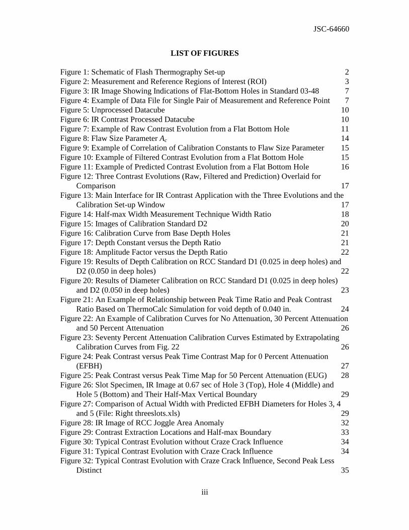
LIST OF FIGURES

Figure 1: Schematic of Flash Thermography Set-up 2

Figure 2: Measurement and Reference Regions of Interest (ROI) 3

Figure 3: IR Image Showing Indications of Flat-Bottom Holes in Standard 03-48 7

Figure 4: Example of Data File for Single Pair of Measurement and Reference Point 7

Figure 5: Unprocessed Datacube 10

Figure 6: IR Contrast Processed Datacube 10

Figure 7: Example of Raw Contrast Evolution from a Flat Bottom Hole 11

Figure 8: Flaw Size Parameter Ac 14

Figure 9: Example of Correlation of Calibration Constants to Flaw Size Parameter 15

Figure 10: Example of Filtered Contrast Evolution from a Flat Bottom Hole 15

Figure 11: Example of Predicted Contrast Evolution from a Flat Bottom Hole 16

Figure 12: Three Contrast Evolutions (Raw, Filtered and Prediction) Overlaid for

Comparison 17

Figure 13: Main Interface for IR Contrast Application with the Three Evolutions and the

Calibration Set-up Window 17

Figure 14: Half-max Width Measurement Technique Width Ratio 18

Figure 15: Images of Calibration Standard D2 20

Figure 16: Calibration Curve from Base Depth Holes 21

Figure 17: Depth Constant versus the Depth Ratio 21

Figure 18: Amplitude Factor versus the Depth Ratio 22

Figure 19: Results of Depth Calibration on RCC Standard D1 (0.025 in deep holes) and

D2 (0.050 in deep holes) 22

Figure 20: Results of Diameter Calibration on RCC Standard D1 (0.025 in deep holes)

and D2 (0.050 in deep holes) 23

Figure 21: An Example of Relationship between Peak Time Ratio and Peak Contrast

Ratio Based on ThermoCalc Simulation for void depth of 0.040 in. 24

Figure 22: An Example of Calibration Curves for No Attenuation, 30 Percent Attenuation

and 50 Percent Attenuation 26

Figure 23: Seventy Percent Attenuation Calibration Curves Estimated by Extrapolating

Calibration Curves from Fig. 22 26

Figure 24: Peak Contrast versus Peak Time Contrast Map for 0 Percent Attenuation

(EFBH) 27

Figure 25: Peak Contrast versus Peak Time Map for 50 Percent Attenuation (EUG) 28

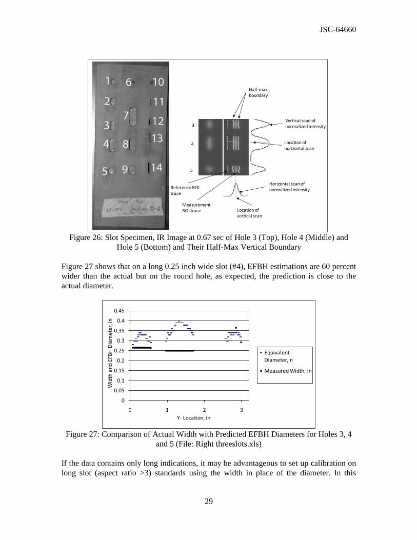
Figure 26: Slot Specimen, IR Image at 0.67 sec of Hole 3 (Top), Hole 4 (Middle) and

Hole 5 (Bottom) and Their Half-Max Vertical Boundary 29

Figure 27: Comparison of Actual Width with Predicted EFBH Diameters for Holes 3, 4

and 5 (File: Right threeslots.xls) 29

Figure 28: IR Image of RCC Joggle Area Anomaly 32

Figure 29: Contrast Extraction Locations and Half-max Boundary 33

Figure 30: Typical Contrast Evolution without Craze Crack Influence 34

Figure 31: Typical Contrast Evolution with Craze Crack Influence 34

Figure 32: Typical Contrast Evolution with Craze Crack Influence, Second Peak Less

Distinct 35

JSC-64660

iv

Figure 33: Contrast Evolution with Craze Crack Influence, No Second Peak 35

Figure 34: Peak Contrast along the Indication 36

Figure 35: Peak Time along the Indication 36

Figure 36: Persistence Energy Time along the Indication 37

Figure 37: EFBH Diameter, Depth and Half-max Width Estimations 37

Figure 38: IR Contrast Diameter and Depth Prediction 38

Figure 39: Comparison of EFBH Diameter and Adjusted 50 Percent Attenuation EUG

Diameter 39

Figure 40: Inverse of Gamma Square Variation along the Y-Location 39

Figure 41: Example of Use of Peak Product Time as a Parameter Related to EFBH/EUG

Diameter 40

Figure 42: Example of Use of Peak Time to Contrast Ratio as a Parameter Related to

EFBH/EUG Depth 40

Figure 43: Typical Schematic of Cross Section of the Specimen 41

Figure 44: Experimental Data of Measured Gap Thickness versus the Width Ratio on

Linear Indications 44

Figure 45: Peak Product Time/Width2.3

versus Gap Thickness on Square Voids Using

ThermoCalc Simulation 45

Figure. 46: Experimental Data of Peak Product Time/Half-max Width2

versus Measured

Gap Thickness on Linear Voids in RCC 45

JSC-64660

1

Flash Infrared Thermography Contrast Data Analysis

Technique

Abstract

This paper provides information on an IR Contrast technique that involves extracting

normalized contrast versus time evolutions from the flash thermography inspection

infrared video data. The analysis calculates thermal measurement features from the

contrast evolution. In addition, simulation of the contrast evolution is achieved through

calibration on measured contrast evolutions from many flat-bottom holes in the subject

material. The measurement features and the contrast simulation are used to evaluate flash

thermography data in order to characterize delamination-like anomalies. The thermal

measurement features relate to the anomaly characteristics. The contrast evolution

simulation is matched to the measured contrast evolution over an anomaly to provide an

assessment of the anomaly depth and width which correspond to the depth and diameter

of the equivalent flat-bottom hole (EFBH) similar to that used as input to the simulation.

A similar analysis, in terms of diameter and depth of an equivalent uniform gap (EUG)

providing a best match with the measured contrast evolution, is also provided. An edge

detection technique called the half-max is used to measure width and length of the

anomaly. Results of the half-max width and the EFBH/EUG diameter are compared to

evaluate the anomaly. The information provided here is geared towards explaining the IR

Contrast technique. Results from a limited amount of validation data on reinforced

carbon-carbon (RCC) hardware are included in this paper.

1. Introduction

Infrared (IR) Flash thermography is a Nondestructive Evaluation (NDE) method used in

the inspection of thin nonmetallic materials such as laminated composites in the

aerospace industry. It is primarily used to detect delamination-like anomalies, although

surface cracks are also detectable to some extent. In most circumstances, a single-sided or

reflection technique is used where the flash lamp (heat source) and the IR camera

(detector) are on the same side of the part (test object) inspected. In some situations, a

through-transmission or two-sided flash thermography technique is used. In the through-

transmission technique, the source and the detector are on the opposite sides of the part.

The area of the part under inspection has constant part thickness in the through-

transmission flash thermography. Maldague1 provides general information on flash

thermography including practical examples and mathematical analysis. Carslaw and

Jaeger2 provide analytical solutions for thermal conduction in an isotropic material for

many cases of heat sources and boundary conditions. Spicer3 provides information on

both theory and applications in active thermography for nondestructive evaluation. This

paper deals only with the single-sided flash thermography.

JSC-64660

2

2. Flash Thermography Equipment

The IR Flash thermography equipment consists of a flash-hood, flash power

supply/trigger unit, flash duration controller, camera data acquisition electronics and a

personal computer (PC). The PC is used for controlling the flash trigger, camera data

acquisition, data display and post processing of the acquired data. The flash-hood is made

from sheet metal. One of the six sides of the hood is open. The side opposite to the open

side has a hole in the center to provide a window for the lens of the IR camera which is

mounted from outside of the hood. The IR camera is focused at the test object (part)

surface located at the hood opening. Two flash lamps are located at the inner wall of the

hood on the camera side. These flash lamps direct the illumination towards the hood

opening where the part is located without directly shining the light into the camera lens.

The hood contains most of the intense flash. See Fig. 1.

IR Camera

Hood

Flash lamp

Opening in back face of hood

Test object

Stand-off

Work bench

Reflector

Glass shield

Figure 1: Schematic of Flash Thermography Set-up

3. One-Sided Flash Thermography Technique

If the test object can be accommodated inside the hood, then it is located at the hood

opening or slightly inside the hood. Otherwise, the part is located slightly outside of the

hood opening. A short duration (e.g. 5 msec), intense (12 kJ) flash is triggered using the

computer keyboard. The data acquisition is triggered a few seconds before the flash and it

continues until the prescribed time. The camera provides a sequence of IR images (or

frames) called the datacube of the part surface taken at the chosen frame rate (e.g. 60 Hz

or 60 frames per sec). The intensity (numerical value) of each pixel in the image is a

function of the surface temperature of the corresponding area on the part at the time of the

image frame. The flash causes the surface to warm up slightly and the heat starts to

JSC-64660

3

dissipate rapidly. The surface cools through thermal radiation, convection and

conduction. It is assumed that the heat conduction within the part is the dominant heat

transfer mode until the temperature gradients within the part become small. At later

times, the heat conduction is of the order of the combined effect of heat convection and

radiation. The IR data acquisition and data analysis utilizes the thermal data in the short

duration immediately after the flash where the thermal dissipation is dominated by the

heat conduction (adabatic process) within the part. Metallic and thin non-metallic

specimens can be often considered as adiabatic, i.e. the convection heat exchange

coefficient value can be assumed zero in these cases. The limit in specimen properties for

considering the adiabatic case is given with the following expression that is well-known

in the heat conduction theory:

0.1.h L

BiK

Here, L is the specimen thickness, K is the specimen conductivity and Bi is the Biot

number.

4. IR Flash Thermography Anomaly Detection

Let us assume that the part is a plate made of a thermally isotropic material with constant

thickness and it fits inside the hood. The plate is supported at the corners on insulating

standoffs and the hood is oriented vertically. If we assume that the flash intensity is

uniform over the plate top surface, then the heat conduction will be in a direction normal

to the part surface in most of the acreage area (area away from edges of the part and flash

boundary). The heat is conducted uniformly from the top surface to the bottom surface of

the plate. The normal heat conduction will be obstructed by an anomaly such as a small

round gapping delamination at the center of a plate, as depicted in Fig. 2. The volume

bounded by the anomaly on one side and the part top surface on the other side is called

the heat trapping volume.

Measurement ROI

Reference ROI

Depth

Testobject

thickness

Flash side

Diameter or width

Delamination or void

Gap

Heat trapping volume

Figure 2: Measurement and Reference Regions of Interest (ROI)

JSC-64660

4

The top surface area surrounding the anomaly cools faster than the top surface (footprint)

area above the anomaly. The IR camera captures the surface temperature image in terms

of the pixel intensity and shows the anomaly as a hot spot (e.g. an area warmer than the

surrounding area) which is about the size and shape of the anomaly footprint. Relative

pixel intensity of the hot spot changes with the time. Deeper anomalies appear at later

times in the IR video compared to the near surface anomalies. After the appearance of an

anomaly in the IR video, its relative pixel intensity continues to increase with time. The

relative pixel intensity of the anomaly reaches a peak at a certain time and then the

relative intensity decays until the indication area temperature and the surrounding area

temperature become equal. Figure 3 shows an IR image of a plate with round flat-bottom

holes (FBH’s) machined from the back side to simulate gapping delaminations of

differing depths. The part continues to cool down to ambient temperature through heat

convection and radiation. If any objects contact the part or the part has significant area

that does not receive the flash, then the heat conduction to unflashed area or to the

contacting object also causes cooling.

5. Flash Thermography IR Data Analysis Using Commercial Software

Commercially available IR data analysis software analyzes the data to detect the

anomalies by providing enhanced processed images. Commercial software EchoTherm4

and Mosaic4 by Thermal Wave Imaging Inc., provide many post-processing options such

as, frame subtraction from other frames, frame averaging, pixel intensity rescaling etc.

They also provide first and second derivative images of the pixel intensity with respect to

the frame number or time. The derivative images are drawn from fitted data. The fitted

data is created by fitting curves in the pixel intensity versus time profile of each pixel.

The pixel intensity (average of one or more neighboring pixels) versus time (T-t) curve

can be displayed in logarithmic (log-log) scale. An ideal temperature-time decay log-log

curve1 on a thick plate with no anomalies is a straight line with a slope of -0.5. The

measured log-log curve on an anomaly would have a constant negative slope for some

time after the flash but at a time related to the heat transit time to the anomaly, the decay

curve would depart from the linear constant slope (see ASTM E 2582). The departure

time or the early appearance time (tappear) can be used to estimate the depth of the

anomaly. The software also allows a calibration of a ruler for measuring the distance

between the pixels and provides the pixel coordinates. Thermofit Pro5 also provides many

of the above image post-processing routines such as derivatives of pixel intensities. This

software also defines a running contrast and normalized contrast. The definition of

Thermofit Pro normalized contrast is different than used in this paper. The Thermofit Pro

software does not define normalized image contrast and the normalized temperature

contrast separately and therefore does not make distinction between the two. Both

EchoTherm and Thermofit Pro implicitly assume that the pixel intensity is proportional to

the surface temperature and is a complete indicator of the surface temperature.

The EchoTherm software provides simple pixel “contrast”, which is defined as the

difference in the pixel intensity of any two selected areas on the test object surface. The

JSC-64660

5

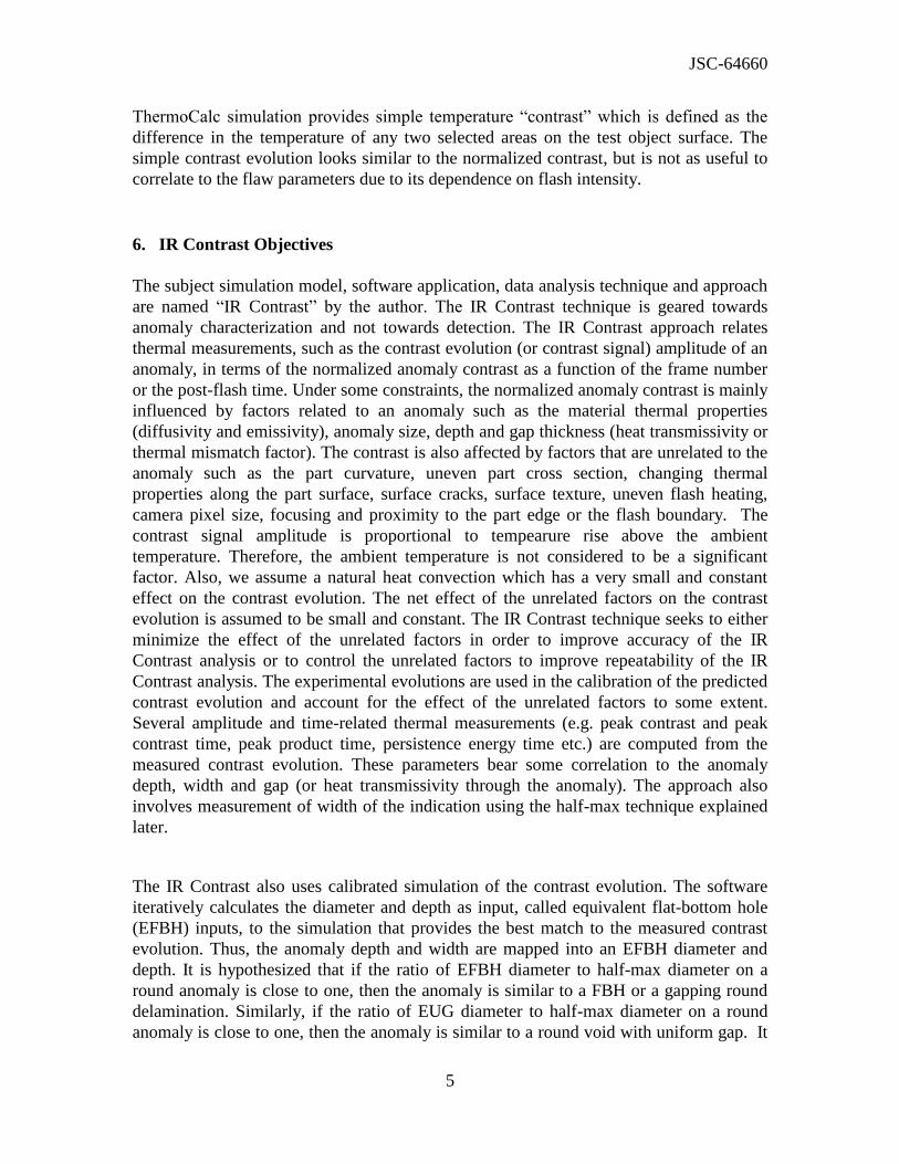
ThermoCalc simulation provides simple temperature “contrast” which is defined as the

difference in the temperature of any two selected areas on the test object surface. The

simple contrast evolution looks similar to the normalized contrast, but is not as useful to

correlate to the flaw parameters due to its dependence on flash intensity.

6. IR Contrast Objectives

The subject simulation model, software application, data analysis technique and approach

are named “IR Contrast” by the author. The IR Contrast technique is geared towards

anomaly characterization and not towards detection. The IR Contrast approach relates

thermal measurements, such as the contrast evolution (or contrast signal) amplitude of an

anomaly, in terms of the normalized anomaly contrast as a function of the frame number

or the post-flash time. Under some constraints, the normalized anomaly contrast is mainly

influenced by factors related to an anomaly such as the material thermal properties

(diffusivity and emissivity), anomaly size, depth and gap thickness (heat transmissivity or

thermal mismatch factor). The contrast is also affected by factors that are unrelated to the

anomaly such as the part curvature, uneven part cross section, changing thermal

properties along the part surface, surface cracks, surface texture, uneven flash heating,

camera pixel size, focusing and proximity to the part edge or the flash boundary. The

contrast signal amplitude is proportional to tempearure rise above the ambient

temperature. Therefore, the ambient temperature is not considered to be a significant

factor. Also, we assume a natural heat convection which has a very small and constant

effect on the contrast evolution. The net effect of the unrelated factors on the contrast

evolution is assumed to be small and constant. The IR Contrast technique seeks to either

minimize the effect of the unrelated factors in order to improve accuracy of the IR

Contrast analysis or to control the unrelated factors to improve repeatability of the IR

Contrast analysis. The experimental evolutions are used in the calibration of the predicted

contrast evolution and account for the effect of the unrelated factors to some extent.

Several amplitude and time-related thermal measurements (e.g. peak contrast and peak

contrast time, peak product time, persistence energy time etc.) are computed from the

measured contrast evolution. These parameters bear some correlation to the anomaly

depth, width and gap (or heat transmissivity through the anomaly). The approach also

involves measurement of width of the indication using the half-max technique explained

later.

The IR Contrast also uses calibrated simulation of the contrast evolution. The software

iteratively calculates the diameter and depth as input, called equivalent flat-bottom hole

(EFBH) inputs, to the simulation that provides the best match to the measured contrast

evolution. Thus, the anomaly depth and width are mapped into an EFBH diameter and

depth. It is hypothesized that if the ratio of EFBH diameter to half-max diameter on a

round anomaly is close to one, then the anomaly is similar to a FBH or a gapping round

delamination. Similarly, if the ratio of EUG diameter to half-max diameter on a round

anomaly is close to one, then the anomaly is similar to a round void with uniform gap. It

JSC-64660

6

is hypothesized that the EFBH depth is an estimation of the anomaly depth if the anomaly

is similar to a gapping delamination or a FBH. Similarly, the EUG depth is an estimation

of the anomaly depth if the anomaly is similar to a void with a uniform gap. The IR

Contrast allows better characterization of the anomaly in terms of anomaly depth and

width and the gap thickness. The IR Contrast application is programmed for many

materials and therefore provides a quick approximate prediction of the contrast on a given

delamination-like anomaly. It can be used as a training tool for the application of flash

thermography.

7. Normalized Contrast Definition

The normalized contrast is defined as,

00

00

RR

RRt

TTTT

TTTTC

, (1)

where, t

C normalized contrast or modulation contrast. It is a function of the post flash

time, t. The time is measured from the moment of the flash (e.g. flash time = 0).

T IR camera pixel intensity at the measurement point (region of interest (ROI))

of the anomaly

RT pixel intensity at the anomaly reference point or ROI,

0T pixel intensity in the measurement ROI of the anomaly before flash,

0

RT pixel intensity of the reference ROI before flash.

Any selected region (point or area) where pixel intensity is measured is referred to as the

region of interest (ROI)

Figures 3 and 4 depict the location of the measurement and reference ROI’s and an

example of a contrast data file.

JSC-64660

7

Reference ROIoutside anomalyarea

Measurement ROI in thecenter of anomaly area

ROI

IR Indications fromdifferent flat bottom holes

Figure 3: IR Image Showing Indications of Flat-Bottom Holes in Standard 03-48

Eq. 1 can be written as,

R

Rt

TT

TTC

, (2)

where, 0TTT pixel intensity rise at the measurement ROI of the anomaly at time

t,

0

RRR TTT pixel intensity rise at the reference ROI at time t.

Column with heading “1” forIR intensity and position of Measurement ROI

Column with heading “2” forIR intensity and position of Reference ROI

Left column gives time in secwith flash time = 0.0 sec

Each row corresponds toone frame e.g.(time, ROI “1” intensity, ROI “2” intensity)

Figure 4: Example of Data File for Single Pair of Measurement and Reference Point

JSC-64660

8

Thus, the normalized IR Contrast is defined as the ratio of the difference in pixel intensity

rise between the anomaly measurement point and the reference point and the sum of the

two pixel intensity rises. This definition is similar to the definition of signal modulation

and the values would range from -1 to +1 in normal situations. In some abnormal

situations the values beyond customary range of -1 to +1 are possible and are outside the

domain of this analysis. In normal measurement situations, the reference area is always

cooler than the anomaly area. Therefore, the contrast shall always be positive. But in

practice, a surface heat gradient caused by factors including the proximity of the anomaly

to the edge of the flash zone or uneven thickness of the cross section may cause the

anomaly to appear cooler at later times compared to temperature of the reference area.

Limits on the proximity of region of interest to a physical boundary, illumination

boundary and part curvature can be determined by investigating the surface pixel intensity

profiles and the contrast evolutions. The pre-flash surface temperature distribution and

emissivity variation also affect the contrast.

Ideally, 00

RTT and Eq. 2 simplifies to,

02TTT

TTC

R

Rt

. (3)

The subtraction of pre-flash pixel intensity and the division by the denominator in the

contrast definition normalizes the numerator. The contrast increases rapidly after the flash

reaching its peak value and then slowly diminishes and achieves a constant level. In

practice, the contrast should ultimately reach a zero value when the temperature equalizes

in the part if we assume a constant and high emissivity (>0.85) and the same pre-flash

temperature in the area of contrast measurement. For low emissivity parts like metals a

high emissivity paint or coating can be applied temporarily to the surface and then the

flash thermography data acquisition can be undertaken.

8. Contrast Extraction

Extraction of the contrast evolution involves choosing the measurement and the reference

points in the datacube. The measurement point is chosen to be the highest intensity pixel.

Usually, the frame chosen for this detection is close to tpeak (defined later). For round

indications, the measurement point is mostly located closed to the center (or centroid) of

the anomaly footprint. For elongated anomalies, several measurement points located close

to the longitudinal centerline of the indication are chosen. This technique yields

repeatable locations of measurement points. Selection of the reference point has many

possibilities in terms of relative location (radial distance and angular orientation) with

respect to the measurement point. Selection of the optimum reference point or points

involves choice of reference points that provides a contrast evolution that is closest to the

ideal contrast evolution. The ideal contrast evolution is defined as the evolution with

maximum possible amplitude from the same anomaly if the anomaly were located in the

JSC-64660

9

acreage area in an ideal material (flat surface, uniform emissivity and diffusivity) under

ideal flash exposure and IR data acquisition conditions as were used during the

calibration. Here, the IR setup seeks uniformity in the pre-flash temperature, even flash

distribution and minimization of the lateral temperature gradients not related to the

anomaly.

One of the techniques involves searching for the reference points that provides leveling of

the contrast evolution. A leveled contrast evolution has the contrast value equal to zero at

later times (ttail defined later). It is desirable to extract a level contrast evolution within

constraints on the relative location and size of the reference point. Combining (e.g.

averaging) of more than one reference point to provide a composite reference point can be

beneficial in leveling the extracted contrast evolution. The IR Contrast application allows

post-extraction (artificial) leveling correction by shifting the contrast evolution up or

down. The post-extraction contrast leveling should be used cautiously with the support of

the validation data. The post-extraction contrast leveling is not likely to be as effective as

the contrast leveling during (or prior to) the contrast extraction. If extraction of the level

contrast evolution is not practical, then other schemes such as fixing the relative

distance/orientation of the reference point can be employed. The scheme provides a

repeatable non-leveled contrast evolution which may be leveled artificially. Here, the

contrast evolution may not provide the most accurate measurements or prediction but is

likely to yield repeatable measurements that differ consistently from ideal contrast

measurements. If the variability of the difference is assessed statistically in a given

application, then it may be possible to apply corrections to the contrast measurements and

estimations.

9. Contrast Imaging

A separate contrast imaging application was written to work with EchoTherm. The

application allows choice of the reference area and then converts the raw datacube into

the contrast datacube using the reference area. The pixel intensity versus time evolution

of each pixel is replaced by the normalized contrast versus time evolution. The contrast

datacube images look similar to raw datacube images. Figure 5 shows a frame from a raw

datacube with pixel intensity versus time curves at selected regions of interest (ROI’s).

Here, all pixels are used as the measurement pixels. Thus, the pixels within the reference

ROI would have a contrast value of zero or close to zero.

JSC-64660

10

Original Data: IR Image Without ROI Points

Original Data: IR Image With ROI Points

ROI Intensity Versus TimeROI Intensity Relative to Reference ROI Versus Time

Reference ROI

Figure 5: Unprocessed Datacube

The chosen reference ROI is shown in Fig. 5. Figure 6 shows a frame from the contrast

datacube with the contrast versus time curves at the selected ROI’s. The contrast datacube

allows a quick view of the contrast evolution and forms the basis for the feature images

based on signal processing (e.g. filtering) and the thermal measurements (e.g. peak time)

defined below.

Contrast Data Image

ROI Intensity versus Frame Number from the Contrast Data-cube

Reference ROI

Selected frame

Figure 6: IR Contrast Processed Datacube

JSC-64660

11

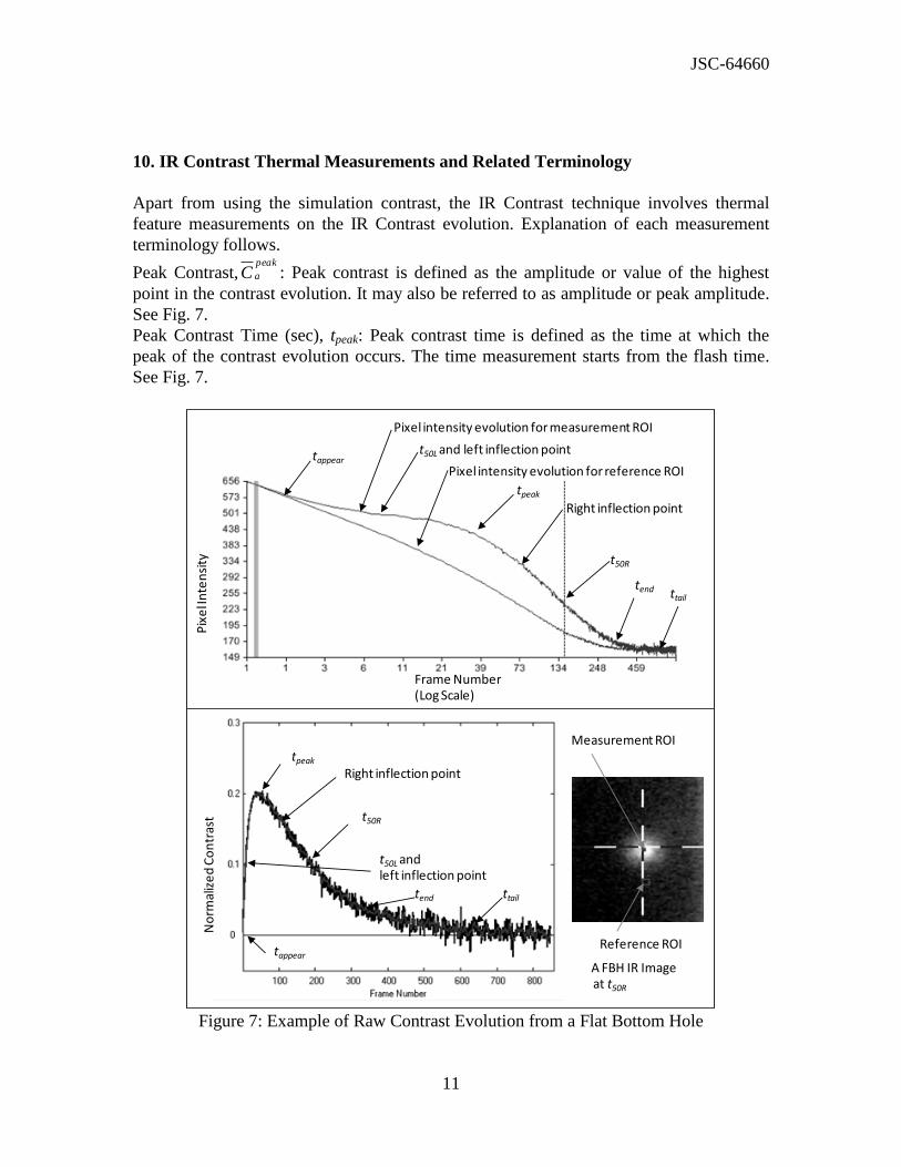
10. IR Contrast Thermal Measurements and Related Terminology

Apart from using the simulation contrast, the IR Contrast technique involves thermal

feature measurements on the IR Contrast evolution. Explanation of each measurement

terminology follows.

Peak Contrast,peak

aC : Peak contrast is defined as the amplitude or value of the highest

point in the contrast evolution. It may also be referred to as amplitude or peak amplitude.

See Fig. 7.

Peak Contrast Time (sec), tpeak: Peak contrast time is defined as the time at which the

peak of the contrast evolution occurs. The time measurement starts from the flash time.

See Fig. 7.

Pix

el I

nte

nsi

ty

Frame Number (Log Scale)

tappeart50Land left inflection point

Right inflection point

tpeak

t50R

tappear

t50Land left inflection point

Right inflection pointtpeak

t50R

No

rmal

ize

d C

on

tras

t

A FBH IR Imageat t50R

tend ttail

tend ttail

Pixel intensity evolution for measurement ROI

Pixel intensity evolution for reference ROI

Reference ROI

Measurement ROI

Figure 7: Example of Raw Contrast Evolution from a Flat Bottom Hole

JSC-64660

12

Fifty Percent Left of Peak Time (Sec), t50L: This is the time at which the 50 percent of

peak contrast occurs before the peak contrast time.

Fifty Percent Right of Peak Time, t50R: This is the time at which the 50 percent of peak

contrast occurs after the peak contrast time.

Ten Percent Right of Peak Time, t10R: This is the time at which the 10 percent of peak

contrast occurs after the peak contrast time.

End Time, tend: This is the time used to determine the right limit point in the time range

for comparison of the measured contrast with the simulation contrast.

peakRend ttt 502 (4)

Tail Time, ttail: Another time used in leveling of the contrast signals or in optimizing the

location of the reference points. The IR Contrast model assumes that the contrast value is

nearly zero at the ttail time.

peakRtail ttt 23 50 (5)

Fifty Percent Persistence Time, t50L-50R: This is the time between t50L and t50R,

LRRL ttt 50505050 . (6)

The times defining the persistence can be different (e.g. t50L-10R).

Withholding Heat Time, twh,50L-50R (sec):

twh,50L-50R = RL

peak

a tC 5050 . (7a)

Withholding heat time is a measure of area under the contrast curve.

Persistence Energy Time, t50L-50R (sec):

50

50

,50 50

R

L

n

a

n

E L R

C

t

, (7b)

where, ν = the frame rate in frames/sec (Hz). n50L and n50R are the frame numbers

corresponding to times t50L and t50R respectively. These frame numbers could be different

as chosen by the user (e.g. n50L to n10R; n50L to npeak; or n1 to n2). Depending upon the

choice of the starting frame number and ending frame number in relation to the peak

time, the integrated times of Eq. (7b) may be denoted as the rise energy time, decay

energy time, etc. In many inspection situations, especially for thin parts, use of the rise

energy time may be appropriate as the rise time is much shorter than the decay times.

JSC-64660

13

Also, if the anomaly depth is expected to be constant, integrating between fixed frames

(e.g. n1 and n2) is useful especially within the rise time window. Both the persistence

energy time and the withholding heat time are related to the heat trapping volume or the

depth and diameter of the anomaly.

Two other important quantities based on the time are defined. These are the peak product

time and the peak time to contrast ratio (or peak time per unit peak contrast). The peak

product time is given by,

peak

product a peakt C t . (8a)

The peak time to contrast ratio is given by,

,

peak

t C peak

a

tt

C . (8b)

From contrast maps (Figs. 24 and 25), it is evident that the peak product time is related to

the diameter of EFBH (or EUG) and peak time to contrast ratio is related to depth of the

EFBH (or EUG). Thus, these measurements are very useful if simulation analysis is not

performed. A smoothed contrast evolution and even simulation fit can provide more

stable detection of the peak point in the contrast evolution compared to the peak detection

on the raw contrast evolution. Therefore, for more repeatable and reliable measurements,

a smoothed evolution or the simulation fit evolution is recommended. In many situations,

the raw evolution may not have a peak corresponding to the subsurface anomaly due to

influence of the texture. In such a situation, use of a simulation fit evolution that is fitted

to the subsurface portion of the raw contrast evolution may be better due to higher

confidence in locating the peak and computing the quantities in Eqs. (8a) and (8b).

11. Contrast Simulation

The contrast simulation uses a quantity called the flaw size parameter, Ac, which is a

function of the anomaly depth and diameter. It is a measure of anomaly size and is shown

in Fig. 8. The peak product time, persistence energy time, withholding heat time and the

peak contrast are measures of the contrast signal strength. Therefore, these measurements

are candidates for conventional probability of detection (POD) analysis where correlation

between the signal response and the flaw size is analyzed. Although the flaw size

parameter Ac is internal to the IR Contrast model, its value is displayed as it plays an

important role in demonstrating correlation between the anomaly size and the IR Contrast

thermal measurements as well as the EFBH predictions. The flaw size parameter can be

used as the flaw size for the POD analysis.

JSC-64660

14

0.1

0.5

0.9

1.30

0.2

0.4

0.6

0.8

1

Flaw

Siz

e P

aram

eter

Depth, in

0.8-1

0.6-0.8

0.4-0.6

0.2-0.4

0-0.2

Diameter, in

Figure 8: Flaw Size Parameter Ac

The IR Contrast simulation assumes that the flaws are located at a shallow depth

compared to the part thickness. It also assumes that the part thickness is considered to be

very thick (>> threshold thickness

7). Calibration parameters such as the depth constant,

diameter constant, amplitude constant and the amplitude factor are used in the simulation

application. The depth constant is used to calibrate for the thermal diffusivity. The

diameter and amplitude constants are functions of the flaw size parameter. The

relationships between the flaw size parameter and the two constants are called the

calibration curves. The calibration curves for the two constants are established by

matching the simulation to the measured contrast of many FBH’s in the material of

interest. These calibration constants are dimensionless. See Fig. 9 for sample calibration

curves.

JSC-64660

15

0

1

2

3

4

5

6

7

8

0 0.2 0.4 0.6 0.8 1

Co

nst

an

ts

Flaw Size Parameter

Diameter Constant

Amplitude Constant

Figure 9: Example of Correlation of Calibration Constants to Flaw Size Parameter

The product of the peak time and persistence time provides a correlation to the product of

depth and diameter. The withholding heat time and persistence energy time capture the

strength of the IR indication to draw attention for further analysis. Shallow anomalies

have shorter persistence but higher amplitude. Deeper anomalies have lower amplitude.

Wider anomalies have longer persistence. The persistence energy time includes part of

the evolution containing the peak amplitude.

Nor

mal

ized

Con

tras

t

Filtered contrast evolution overlaid on the raw evolution

Raw contrast evolution

Frame Number

Figure 10: Example of Filtered Contrast Evolution from a Flat Bottom Hole

The raw contrast data contains the camera noise. The signal can be filtered by a signal

processing routine to improve the IR Contrast calculations. The filtered contrast is shown

JSC-64660

16

in gray and the raw contrast is shown in black in Fig. 10. See also Fig. 13 which is in

color. Figure 11 shows the predicted contrast curve that provides the best match to the

measured contrast evolution. The EFBH depth and diameter input to the simulation

providing the best match to measured contrast data is obtained in an automated way. The

IR Contrast application calculates the approximate depth and diameter of the EFBH

directly based on the peak contrast, peak contrast time and other times including t50L, t50R

and t10R. The simulation matching provides an indirect method of assessing the EFBH

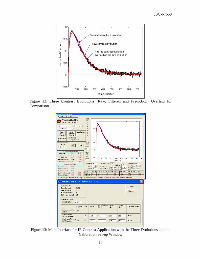
depth and diameter. Figure 12 shows the raw contrast, filtered contrast and the simulation

contrast evolutions plotted on the same graph. See also Fig. 13 which is in color.

No

rma

lize

d C

on

tra

st

Frame Number

Figure 11: Example of Predicted Contrast Evolution from a Flat Bottom Hole

Figure 13 shows the main interface window of the IR Contrast application with the three

contrast evolutions. The differences between the measured data and the simulation are

calculated and are indicated in the lower right of the application window. Numbers in

black are based on the calculations on the raw contrast evolution. Numbers in red are

based on the calculations of the filtered contrast evolution. Numbers in purple relate to

the predicted contrast evolution.

JSC-64660

17

Nor

mal

ized

Con

tras

t

Filtered contrast evolution overlaid on the raw evolution

Raw contrast evolution

Simulated contrast evolution

Frame Number

Figure 12: Three Contrast Evolutions (Raw, Filtered and Prediction) Overlaid for

Comparison

Figure 13: Main Interface for IR Contrast Application with the Three Evolutions and the

Calibration Set-up Window

JSC-64660

18

12. Half-max Width Estimation

The width of the indications can be directly measured from the IR data frame that

provides the peak in the intensity. The pixel intensities along a line drawn across the

linear indication or through the center of a circular indication are plotted against the pixel

position. The pixel coordinates at 50 percent of the peak intensity on the right and left of

the peak intensity location are located. Pixels between the left 50 percent peak and right

50 percent peak are counted and converted to length by multiplying by the pixel size on

the part to obtain an approximate measure of the anomaly width. This technique is called

the half-max width measurement technique. See Fig. 14. The technique can be applied to

normalized evolutions obtained by subtracting the pre-flash pixel intensity. Also, the

choice of frame for the measurement is recommended to be between t50L and tpeak. The

percent level itself may be different than 50 percent to make the boundary estimations

less or more conservative. The half-max approach is limited by the spatial noise. Thus,

the half-max intensity to the spatial noise ratio shall be more than 2 to 3 times for

meaningful boundary estimation. Resolution of the half-max pixel can be improved by

interpolation.

Max Intensity

50% of max

Pixel intensity plotted belowalong this line

Half max widthReference

MeasurementReference

Measuring tapefor lengthcalibration

Pixel Number

Pix

el I

nte

nsi

ty

Crack

Figure 14: Half-max Width Measurement Technique Width Ratio

JSC-64660

19

In order to compare the EFBH estimation with the observed width, a quantity called the

width ratio is introduced. Width Ratio (ψ, psi) is defined as the ratio of the simulation

estimation EFBH diameter to the measured half-max width.

hm

EFBHEFBH

w

D

(9)

The ψ ratio is designed to be close to 1 for calibration FBH’s. If the anomaly is not like a

gapping delamination such that the heat is partially conducted or transmitted through the

anomaly, then the EFBH estimation is expected to be smaller. Therefore, ψ is

hypothesized to correlate to the gap thickness or the degree of heat transmission through

the anomaly. The heat transmission through an anomaly occurs due to the contact

between the delamination faces, the bridging of material in the delamination gap or due to

a very thin air gap. It is hypothesized that a ratio close to 1 on a round delamination

implies that the indication is similar to a flat-bottom hole or a gapping delamination.

Lower values of the width ratio will have more inaccuracies in the depth assessment due

to greater mismatch between shapes of the measured contrast evolution and the simulated

contrast evolution.

13. Amplitude Ratio

In order to compare the EFBH estimation with the measured half-max width, a quantity

called the amplitude ratio is introduced. Similar to the width ratio, this ratio is intended to

evaluate heat transmissivity of the anomaly. If a delamination has an intermittent contact

between the faces, the heat will transmit through the delamination. The heat transmission

results in lowering of the peak contrast value compared to that from the same size FBH.

The overall shape and the peak time are not affected because the normal and lateral transit

times remain the same. Here, the half-max width (whm) is used as a diameter input to the

simulation. The depth input to simulation and the amplitude ratio input to the simulation

are adjusted to match the measured contrast. The amplitude ratio, denoted by ζ (zeta), is

given by,

peak

e

peak

a

C

C , (10)

where peak

eC is the estimated peak contrast using the half-max width and depth providing

a match with the peak time. The amplitude ratio compares the peak contrast (amplitude)

of the measured anomaly with the peak contrast of a flat-bottom hole with the same depth

and diameter. Thus, the amplitude and width ratio values of a round delamination close to

1 would imply that the anomaly is similar to a FBH. A lower amplitude ratio or width

ratio value would imply increased heat transmission due to the material bridging, contact

within the anomaly or thin air gap. The material bridging provides adherence of the

material above the anomaly but a mere contact may not. Therefore, the amplitude ratio

may not always correlate to the material adherence strength.

The width ratio and the amplitude ratio approach are further developed into equivalent

uniform gap (attenuation) mapping. The measured signal can be analyzed to provide the

JSC-64660

20

size and depth of an equivalent FBH or the size and depth of a uniform equivalent gap. In

this approach the gap thickness can be estimated within limitations.

14. Calibration Steps in the IR Contrast Application

Calibration steps for the IR contrast application are provided in the appendix.

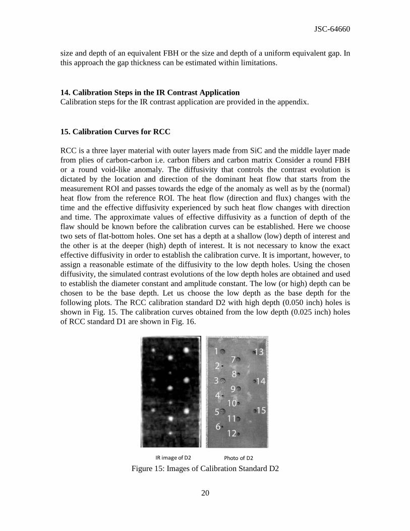
15. Calibration Curves for RCC

RCC is a three layer material with outer layers made from SiC and the middle layer made

from plies of carbon-carbon i.e. carbon fibers and carbon matrix Consider a round FBH

or a round void-like anomaly. The diffusivity that controls the contrast evolution is

dictated by the location and direction of the dominant heat flow that starts from the

measurement ROI and passes towards the edge of the anomaly as well as by the (normal)

heat flow from the reference ROI. The heat flow (direction and flux) changes with the

time and the effective diffusivity experienced by such heat flow changes with direction

and time. The approximate values of effective diffusivity as a function of depth of the

flaw should be known before the calibration curves can be established. Here we choose

two sets of flat-bottom holes. One set has a depth at a shallow (low) depth of interest and

the other is at the deeper (high) depth of interest. It is not necessary to know the exact

effective diffusivity in order to establish the calibration curve. It is important, however, to

assign a reasonable estimate of the diffusivity to the low depth holes. Using the chosen

diffusivity, the simulated contrast evolutions of the low depth holes are obtained and used

to establish the diameter constant and amplitude constant. The low (or high) depth can be

chosen to be the base depth. Let us choose the low depth as the base depth for the

following plots. The RCC calibration standard D2 with high depth (0.050 inch) holes is

shown in Fig. 15. The calibration curves obtained from the low depth (0.025 inch) holes

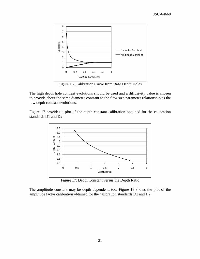
of RCC standard D1 are shown in Fig. 16.

IR image of D2 Photo of D2 Figure 15: Images of Calibration Standard D2

JSC-64660

21

0

1

2

3

4

5

6

7

8

0 0.2 0.4 0.6 0.8 1

Con

stan

ts

Flaw Size Parameter

Diameter Constant

Amplitude Constant

Figure 16: Calibration Curve from Base Depth Holes

The high depth hole contrast evolutions should be used and a diffusivity value is chosen

to provide about the same diameter constant to the flaw size parameter relationship as the

low depth contrast evolutions.

Figure 17 provides a plot of the depth constant calibration obtained for the calibration

standards D1 and D2.

2.5

2.6

2.7

2.8

2.9

3

3.1

3.2

3.3

0 0.5 1 1.5 2 2.5 3

De

pth

Co

nst

an

t

Depth Ratio

Figure 17: Depth Constant versus the Depth Ratio

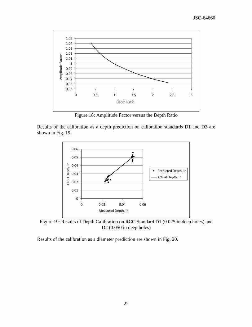
The amplitude constant may be depth dependent, too. Figure 18 shows the plot of the

amplitude factor calibration obtained for the calibration standards D1 and D2.

JSC-64660

22

0.95

0.96

0.97

0.98

0.99

1

1.01

1.02

1.03

1.04

1.05

0 0.5 1 1.5 2 2.5 3

Am

plit

ud

e F

act

or

Depth Ratio

Figure 18: Amplitude Factor versus the Depth Ratio

Results of the calibration as a depth prediction on calibration standards D1 and D2 are

shown in Fig. 19.

0

0.01

0.02

0.03

0.04

0.05

0.06

0 0.02 0.04 0.06

EFB

H D

ep

th, i

n

Measured Depth, in

Predicted Depth, in

Actual Depth, in

Figure 19: Results of Depth Calibration on RCC Standard D1 (0.025 in deep holes) and

D2 (0.050 in deep holes)

Results of the calibration as a diameter prediction are shown in Fig. 20.

JSC-64660

23

0

0.05

0.1

0.15

0.2

0.25

0.3

0.35

0.4

0.45

0 0.2 0.4 0.6

EFB

H D

iam

eter

, in

Measured Diameter, in

Predicted Diameter, in

Actual Diameter, in

Actual diameter points joined in a line for comparison

Figure 20: Results of Diameter Calibration on RCC Standard D1 (0.025 in deep holes)

and D2 (0.050 in deep holes)

16. Calibration for Specified Attenuation (%μ) for a Thin Delamination

It is assumed that an air gap exists in the delamination. The heat transmits through the air

gap. Thin gaps transmit heat by air conduction. Thick gaps transmit heat by convection.

The radiative heat transfer is mostly independent of the gap thickness and is not a major

contributor to the heat transmission. Higher contact pressure at the gap interface provides

larger contact area. Therefore, the contact pressure affects the rate of heat conduction.

As the energy is transmitted through the gap, the registered peak amplitude is reduced

compared to the amplitude from a corresponding FBH. The calibration curves for a

uniform thin gap are different from that of a corresponding FBH. Ideally, physical

reference standards with known and uniform gaps shall be fabricated to establish the

calibration curves for known gaps. However, using simulation, it can be shown that a gap

of less than 0.010 inch is needed to reduce the contrast amplitude significantly. While

very thin gaps can be modeled in the simulation, it may be impractical to create controlled

gaps that are less than 0.001 inch in thickness to study the effect of gap thickness on the

contrast evolution.

An alternate approximate approach is to use a ThermoCalc (or other) simulation. In the

ThermoCalc simulation, we choose many void widths at the same low (base) depth. We

choose a different gap thickness for each run. We choose a large gap thickness (0.150 in)

to represent the case of a FBH. We choose several other values with the lowest gap

thickness at about 0.0005 in. We calculate the peak time ratio and the peak amplitude

ratio with respect to the peak time and amplitude of the FBH. The peak time ratio is

plotted against peak amplitude ratio for each hole with each gap thickness. Here we

choose a desired amplitude attenuation level e.g. 30 percent. The case study (Sec. 20)

indicates the attenuation value from 0 percent to approximately 50 percent on the chosen

sample. From the plot, we read the value of the peak time ratio for the chosen amplitude

JSC-64660

24

ratio. We create a table of the peak time ratio for the given gap size. We use the IR

Contrast application simulated contrast evolution (in calibration mode) to note the peak

amplitude and peak time for each void width. We compute the 30 percent attenuation

amplitude by multiplying by 0.7 (1.0 minus peak amplitude ratio). We calculate the

corresponding peak frame by multiplying the FBH peak frame (IR Contrast simulation)

by the peak time ratio. Now we choose the “un-calibrated” mode to input trial values for

the calibration constants that provide the best match with the calculated peak frame and

peak amplitude.

The real delaminations may have thin gaps and the contrast evolution is attenuated. The

relationship between the peak time and peak contrast can be studied by using ThermoCalc

simulation for many void thicknesses that range from very thin (0.0005 in thick) to very

thick (e.g. 0.150 in). The thick voids can be considered to be like a flat-bottom hole. The

contrast evolutions for the FBH’s of various sizes can be used as the basis to compute the

peak contrast (amplitude) ratio and the peak time ratio for the corresponding hole widths

for each gap thickness. Here, we make an assumption that the ThermoCalc simulation can

provide acceptable correlation between the peak contrast ratio and the peak time ratio for

a material with known properties. See Fig. 21.

0

0.1

0.2

0.3

0.4

0.5

0.6

0.7

0.8

0.9

1

1.1

0 0.1 0.2 0.3 0.4 0.5 0.6 0.7 0.8 0.9 1

Pe

ak

Tim

e R

ati

o

Peak Contrast Ratio

Gamma = 4.9

Gamma = 6.9

Gamma = 8.9

Gamma = 10.8

Gamma = 12.8

g = 0.0005 in

Figure 21: An Example of the Relationship between Peak Time Ratio and Peak Contrast

Ratio Based on ThermoCalc Simulation for a void depth of 0.040 in.

Using the above results we can establish a correlation between the gamma (void width

divided by void depth) and the peak time ratio for a chosen attenuation in the simulated

peak contrast. The fifty percent attenuation corresponds to an air gap thickness of

approximately 0.001 in. The attenuation is similar to the amplitude ratio ζ (zeta). While

the attenuation is used to compare the peak contrasts of the simulated evolutions,

JSC-64660

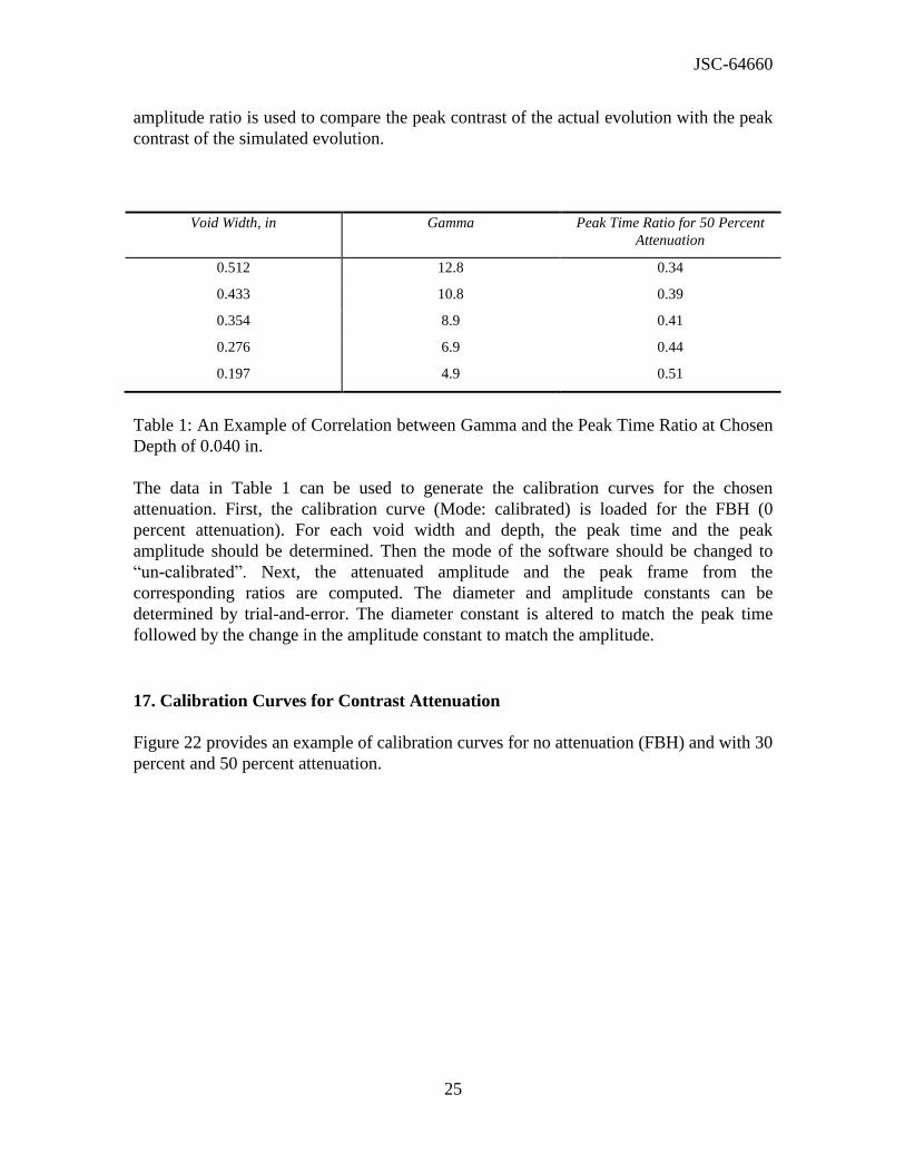
25

amplitude ratio is used to compare the peak contrast of the actual evolution with the peak

contrast of the simulated evolution.

Void Width, in Gamma Peak Time Ratio for 50 Percent

Attenuation

0.512 12.8 0.34

0.433 10.8 0.39

0.354 8.9 0.41

0.276 6.9 0.44

0.197 4.9 0.51

Table 1: An Example of Correlation between Gamma and the Peak Time Ratio at Chosen

Depth of 0.040 in.

The data in Table 1 can be used to generate the calibration curves for the chosen

attenuation. First, the calibration curve (Mode: calibrated) is loaded for the FBH (0

percent attenuation). For each void width and depth, the peak time and the peak

amplitude should be determined. Then the mode of the software should be changed to

“un-calibrated”. Next, the attenuated amplitude and the peak frame from the

corresponding ratios are computed. The diameter and amplitude constants can be

determined by trial-and-error. The diameter constant is altered to match the peak time

followed by the change in the amplitude constant to match the amplitude.

17. Calibration Curves for Contrast Attenuation

Figure 22 provides an example of calibration curves for no attenuation (FBH) and with 30

percent and 50 percent attenuation.

JSC-64660

26

0

0.5

1

1.5

2

2.5

3

3.5

4

4.5

0 0.2 0.4 0.6 0.8 1

Cal

ibra

tion

Con

stan

ts

Flaw Size Parameter

Diameter Constant, No Attenuation

Amplitude Constant, No Attenuation

Diameter Constant,

30% Attenuation

Amplitude Constant,

30% Attenuation

Diameter Constant,

50% Attenuation

Amplitude Constant, 50% Attenuation

Figure 22: An Example of Calibration Curves for No Attenuation, 30 Percent Attenuation

and 50 Percent Attenuation

Seventy percent attenuation calibration curves can be calculated by extrapolating previous

curves. The corresponding calibration curves are shown in Fig. 23.

0

0.5

1

1.5

2

2.5

3

3.5

4

4.5

0 0.2 0.4 0.6 0.8 1

Co

nst

ants

Flaw Size Parameter

Diameter Constant, 70% Attenuation

Amplitude Constant, 70% Attenuation

Diameter Constant, No Attenuation

Amplitude Constant, No Attenuation

Figure 23: Seventy Percent Attenuation Calibration Curves Estimated by Extrapolating

Calibration Curves from Fig. 22

JSC-64660

27

18. Contrast Maps for the Attenuated Calibrations

Figure 24 shows an example of a map of the peak contrast and peak time for flat-bottom

holes in RCC. The map is also known as the contrast map. The map indicates the IR

Contrast prediction region. At the upper left corner and lower right corner the prediction

is not accurate in terms of the diameter. Also, the low amplitude evolutions have higher

error in the prediction.

0

0.1

0.2

0.3

0.4

0.5

0.6

0.7

0.8

0 0.5 1 1.5 2

Peak

Con

tras

t

Peak Time, sec

0.125 inch

Diameter0.250 inch Diameter0.375 inch Diameter0.500 inch Diameter0.075 inch Depth

0.050 inch Depth

0.025 inch Depth

0.015 inch Depth

Figure 24: Peak Contrast versus Peak Time Contrast Map for 0 Percent Attenuation

(EFBH)

Figure 25 shows an example of a map of the peak contrast and peak time for uniform

round thin gaps with 50 percent attenuation in RCC. For thin gaps with 50 percent

attenuation, the contrast map indicates much lower peak contrast and peak times. The

contrast application can choose FBH calibration or the percent attenuation calibration.

When finding a simulation match on the contrast evolutions from a FBH, the percent

attenuation calibration may not be able to find a match. Similarly, when finding a

simulation match on contrast evolutions from thin delaminations, the FBH calibration

may not be able to find a match. The degree of match can be viewed as contrast plots and

quantified as the summation of the square of the difference over a range of chosen frames.

It is postulated that the 50 percent attenuation is a good approximation for gaps of the

order of 0.001 in based on the simulation data from Fig. 21. The map indicates severe

contrast attenuation at 0.5 sec for the 50 percent attenuation.

Figure 25 indicates that compared to the contrast map for the FBH’s, the near surface

delaminations attenuate relatively less than the deeper delaminations. The air-gap at the

delamination is similar to a contact resistance or a thermal mismatch factor between

layers. The thermal mismatch factor between two layers is based on the ratio of

effusivities of the two materials. The thermal mismatch between the top layer and the

next layer may vary periodically along the interface in a laminated structure which uses

fabric and matrix. Similarly, the emissivity and diffusivity of the top layer may vary

periodically along the surface. The variation in diffusivity, emissivity and mismatch

factor between the top two layers as well as the surface texture or roughness pattern is

JSC-64660

28

referred to as the surface/near surface thermal texture. Figure 25 implies that a hot spot in

the IR image of the surface texture would provide an early peak. Here, we assume that

measurement ROI size is smaller than or equal to the width of the hot spot. Similarly, a

cold spot should provide a negative peak in the contrast profile. Thus, in detection of

delaminations, it is important to properly interpret the early time peaks as possibly due to

surface texture. These indications may superimpose on the signal from shallow

delaminations reducing resolution in evaluating shallow delaminations.

0

0.1

0.2

0.3

0.4

0.5

0.6

0 0.2 0.4 0.6 0.8

Peak

Con

tras

t

Peak Time, s

0.125 in Diameter

0.250 in Diameter

0.375 in Diameter

0.500 in Diameter

0.005 in Depth

0.015 in Depth

0.025 in Depth

0.050 in Depth

0.075 in Depth

Figure 25: Peak Contrast versus Peak Time Map for 50 Percent Attenuation (EUG)

For long indications the EFBH or EUG diameter estimations are higher than the actual

width due to the length to width aspect ratio being greater than 1. The effect can be

studied on a slot standard. Figure 26 shows a slot standard and IR image of holes 3, 4 and

5. The figure also illustrates the half-max boundary detection. The half-max boundary

closely matches the actual vertical edges of the three anomalies.

JSC-64660

29

Location of vertical scan

Location of horizontal scan

Vertical scan of normalized intensity

Horizontal scan of normalized intensity

Half-max boundary

Measurement ROI trace

Reference ROI trace

3

4

5

Figure 26: Slot Specimen, IR Image at 0.67 sec of Hole 3 (Top), Hole 4 (Middle) and

Hole 5 (Bottom) and Their Half-Max Vertical Boundary

Figure 27 shows that on a long 0.25 inch wide slot (#4), EFBH estimations are 60 percent

wider than the actual but on the round hole, as expected, the prediction is close to the

actual diameter.

0

0.05

0.1

0.15

0.2

0.25

0.3

0.35

0.4

0.45

0 1 2 3

Wid

th a

nd

EFB

H D

iam

ete

r, in

Y- Location, in

Equivalent

Diameter,in

Measured Width, in

Figure 27: Comparison of Actual Width with Predicted EFBH Diameters for Holes 3, 4

and 5 (File: Right threeslots.xls)

If the data contains only long indications, it may be advantageous to set up calibration on

long slot (aspect ratio >3) standards using the width in place of the diameter. In this

JSC-64660

30

situation, correction for the length effect will not be needed for most of the length of the

indication except near the ends.

19. Similarities and Differences between Flash Thermography IR Contrast Analysis

and Ultrasonic Pulse Echo Analysis

It is important to point out similarities and differences between the pulse-echo ultrasonic

A-scan analysis and the contrast evolution analysis. The IR Contrast algorithm is used to

analyze delamination-like anomalies. The IR Contrast concept is similar to flaw sizing in

ultrasonic inspection of wrought metal. In the ultrasonic technique, usually a plate of

wrought metal is inspected for internal separations. The part may be immersed in water

along with the ultrasonic transducer.

A longitudinal ultrasonic pulse is triggered at the transducer and is transmitted through

water to the part where a portion of the ultrasonic pulse is reflected and a portion is

transmitted into the part. The pulse reflects off the anomaly and some of the reflected

pulse energy, after passing through the water-to-metal interface, is received back by the

transducer. The ultrasonic instrument provides an A-scan display. The A-scan shows the

waveform of the received pulse. The horizontal or X-axis is the time of the waveform.

The X-axis can be calibrated in distance of length of the one-way sound-path of the pulse

reflections from the top surface of the part. This distance corresponds to the depth of the

reflector from the top surface of the part. The beginning portion of the A-scan has the

waveform of the initial pulse applied to the transducer. The remaining portion of the A-

scan indicates the reflected pulse energy. The reflected pulse amplitude is affected by the

depth and size of the reflector.

Flat-bottom hole reference standards are used to calibrate the inspection technique for

depth and depth-amplitude correlation. In addition, area-amplitude correlations can also

be established externally.

The ultrasonic pulse has a beam width. The aperture and curvature of the transducer

influences the beam width. The beam width usually changes with the distance from the

transducer. For an unfocused transducer, the aperture primarily controls the amount of

energy received. For a focused transducer, both beam width at the reflector and the

aperture influence the amount of energy received.

The IR Contrast evolution shows some similarities with the ultrasonic pulse-echo A-scan,

especially when the ultrasonic signal is rectified on the positive side and the envelope

mode is used. The horizontal axis is time in both cases. The peak time in both cases

relates to the depth of the anomaly from the part surface. In the ultrasonic technique, the

ultrasound material velocity is used to convert peak time to reflector depth by multiplying

the one-way transit time observed in the A-scan by the velocity of ultrasound. In the IR

Contrast analysis, material heat diffusivity is primarily used to convert the peak time to

depth although width of the contrast envelope (persistence time) also affects this

JSC-64660

31

correlation. Both techniques use flat-bottom hole standards for amplitude/depth

calibration. In the ultrasonic technique, the depth amplitude factor calibration can be

incorporated in real-time such that the chosen area of the flaw provides the same

amplitude at a range of flaw depths. In the IR Contrast analysis, the calibration is applied

to a separate simulated contrast evolution. The actual contrast evolution is not altered by

the calibration. Similar to the ultrasonics, the area/amplitude correlation is also

established for the IR Contrast. Typically, FBH at two depths of interest are chosen.

As the flaw size increases, the amplitude of reflected ultrasonic pulse increases but as the

size of the flaw grows comparable to the aperture or the beam width at the flaw, the

growth in the amplitude slows and reaches a saturation value. A similar relationship is

observed for very high gamma (diameter/depth) flaws in the IR Contrast evolution. The

contrast signature is not affected by further increase in the gamma. For elongated flaws,

typically the growth in length beyond two times of the width does not increase the IR

Contrast peak amplitude significantly for shallow flaws.

Tighter delaminations transmit ultrasound depending upon the amount of contact pressure

or bonding. Tighter delaminations conduct heat depending upon the amount of the

contact pressure. While thin delaminations can conduct and convect heat, they cannot

conduct detectable ultrasound at megahertz frequencies. If the there is no contact pressure

or bond, very little ultrasound energy is transmitted.

In the ultrasonic pulse-echo technique, a single delamination may register multiple echoes

in the A-scan. In the IR Contrast, only one envelope is registered by a single

delamination. In the case of multiple delaminations of about the same size that are

stacked, only the nearest delamination is detected by both ultrasonics and the flash IR

technique. In a special case where a vertical surface crack or cracks connect to a

subsurface delamination, two peaks may be observed in the contrast evolution as

described in the following case study. The first peak is usually very sharp (short

persistence time) and is due to the surface cracks or surface (or near-surface) texture. In

graphite-epoxy laminates, the weave pattern of the top layer may provide surface texture.

Depending upon the pixel location a sharp peak or a sharp dip may be observed in earlier

times.

In ultrasonics, the near surface resolution is limited by the surface roughness, ultrasound

wavelength and the beam diameter. In flash thermography, the surface texture reduces

near-surface resolution. In order to image the texture satisfactorily, the IR image pixel

size should be less than a third of the texture wavelength (or the width of the hot spot or

the stripe in the IR image). In order to detect a thin gap sub-surface delamination under

the texture, the width of the sub-surface delamination should be more than the texture

wavelength and it should not be aligned with the texture.

The second peak has lower amplitude and longer persistence time; and is due to the

delamination. In some situations the two peaks may merge into one envelope with only

one distinct peak location which is heavily influenced by presence of the crack. Echoes

JSC-64660

32

from vertical cracks are very small in the longitudinal wave pulse-echo ultrasonic

inspection compared to the echo from a delamination.

20. Case Study: RCC Joggle Area Test Pieces with Subsurface Delaminations

We analyze an RCC test piece with a linear (along vertical or Y-direction) delamination.

Figure 28 shows an IR image of a test piece (6L-2A_25-30y_ss_200P06L004). The two

white dots in the center indicate near surface delaminations known as flakes.

Flake locations

Figure 28: IR Image of RCC Joggle Area Anomaly

Figure 29 shows the half-max boundary in white. The gray line between the left and right

half-max boundaries indicates the high intensity locations chosen as the measurement

points and the leftmost gray line shows the reference locations. A contrast data file is

extracted based on the measurement and reference points and is analyzed by the IR

Contrast application for diameter and depth.

JSC-64660

33

Left half-max boundary

Right half-max boundary

Reference ROI location trace

Measurement ROI location trace

Figure 29: Contrast Extraction Locations and Half-max Boundary

Figure 30 shows a typical contrast evolution at a chosen measurement pair (measurement

ROI and corresponding reference ROI) when craze cracks are not present close to the

measurement ROI.

JSC-64660

34

No

rmal

ized

Co

ntr

ast

Single peak

Frame Number

Figure 30: Typical Contrast Evolution without Craze Crack Influence

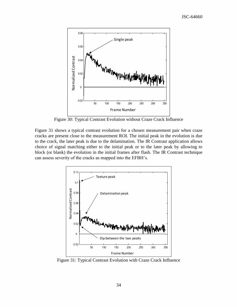
Figure 31 shows a typical contrast evolution for a chosen measurement pair when craze

cracks are present close to the measurement ROI. The initial peak in the evolution is due

to the crack, the later peak is due to the delamination. The IR Contrast application allows

choice of signal matching either to the initial peak or to the later peak by allowing to

block (or blank) the evolution in the initial frames after flash. The IR Contrast technique

can assess severity of the cracks as mapped into the EFBH’s.

No

rma

lize

d C

on

tra

st

Texture peak

Delamination peak

Frame Number

Dip between the two peaks

Figure 31: Typical Contrast Evolution with Craze Crack Influence

JSC-64660

35

The craze cracks may be connected to the delamination and the initial and later peaks may

get merged as shown in Figs. 32 and 33.

Nor

mal

ized

Con

tras

t

Dip less prominent

Frame Number

Texture peak

Figure 32: Typical Contrast Evolution with Craze Crack Influence, Second Peak Less

Distinct

No

rmal

ized

Co

ntr

ast

Dip not present

Frame Number

Figure 33: Contrast Evolution with Craze Crack Influence, No Second Peak

Figure 34 shows the peak contrast plot. Two peaks at 1.8 in and 2.8 in are due to flake

spots. The peak contrast is strongly related to the local width of the linear anomaly.

JSC-64660

36

0.01

0.1

1

0 1 2 3 4 5 6

Peak

Con

tras

t

Y-Location, in

Figure 34: Peak Contrast along the Indication

Figure 35 shows the peak time plot. In most of the region the peak time is less than 0.5

sec. In some locations it is greater than 0.5 sec. The peak time is strongly related to the

local depth of the linear anomaly.

0.01

0.1

1

10

0 1 2 3 4 5 6

Pea

k Ti

me,

sec

Y-Location, in

Figure 35: Peak Time along the Indication

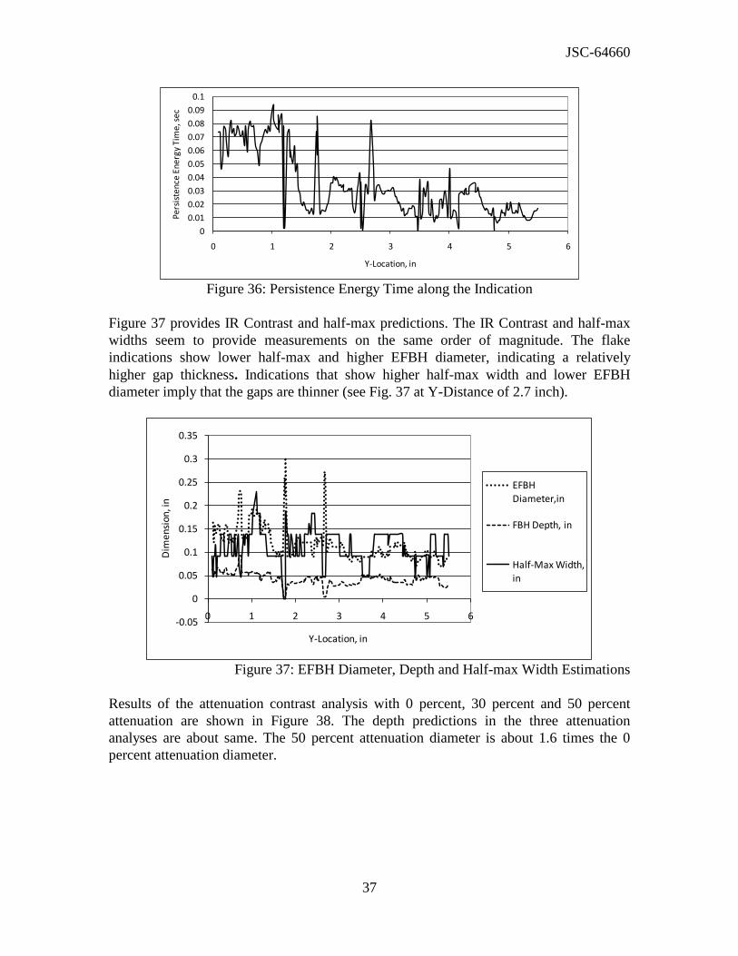
Figure 36 shows the persistence energy time. It shows the two flake peaks at 1.8 inch and

2.8 inch. The plot indicates relatively high persistence energy time from 0 in to 1in. The

persistence energy time is strongly related to the local width of the anomaly.

JSC-64660

37

0

0.01

0.02

0.03

0.04

0.05

0.06

0.07

0.08

0.09

0.1

0 1 2 3 4 5 6

Pe

rsis

ten

ce E

ne

rgy

Tim

e, s

ec

Y-Location, in

Figure 36: Persistence Energy Time along the Indication

Figure 37 provides IR Contrast and half-max predictions. The IR Contrast and half-max

widths seem to provide measurements on the same order of magnitude. The flake

indications show lower half-max and higher EFBH diameter, indicating a relatively

higher gap thickness. Indications that show higher half-max width and lower EFBH

diameter imply that the gaps are thinner (see Fig. 37 at Y-Distance of 2.7 inch).

-0.05

0

0.05

0.1

0.15

0.2

0.25

0.3

0.35

0 1 2 3 4 5 6

Dim

ensi

on, i

n

Y-Location, in

EFBH Diameter,in

FBH Depth, in

Half-Max Width, in

Figure 37: EFBH Diameter, Depth and Half-max Width Estimations

Results of the attenuation contrast analysis with 0 percent, 30 percent and 50 percent

attenuation are shown in Figure 38. The depth predictions in the three attenuation

analyses are about same. The 50 percent attenuation diameter is about 1.6 times the 0

percent attenuation diameter.

JSC-64660

38

0

0.1

0.2

0.3

0.4

0.5

0.6

0.7

0 1 2 3 4 5 6 7

Dim

ensi

on, i

n

Y-Location, in

EFBH Diameter,in

FBH Depth, in

Equivalent Diameter- 30% Attenuation,in

Equivalent Depth-30% Attenuation, in

Equivalent Diameter - 50 %

Attenuation,in

Equivalent Depth - 50% Attenuation,

in

Figure 38: IR Contrast Diameter and Depth Prediction

As expected, the analysis with thinner gaps shows higher diameter estimation. Since the

indication is long, the EFBH and attenuation diameters are expected to be approximately

two times of actual width. The delamination is not like a flat-bottom hole but is more like

a thin gap delamination. We would assume that the delamination is close to 50 percent

attenuation (or a gap of about 0.001 in). Therefore, to obtain an approximate estimate of

width we divide the EUG diameter by about 1.6 (0.250 inch wide delamination at 0.040

in depth). The comparison is shown in Fig. 39. The EFBH and the adjusted 50 percent

attenuation EUG diameter estimations are in good agreement implying EFBH estimations

on the long RCC indications may provide comparable estimations to 50 percent

attenuation measurements with adjustment for the aspect ratio.

Indications that have about the same value for both the EFBH diameter and the half-max

width (or the adjusted 50 percent attenuation width) indicate that the gap thickness

assumed in the 50 percent attenuation analysis is applicable. The attenuation analysis is

based on use of thermal simulation, assumed delamination depth and expected width of a

longitudinal delamination. The EFBH analysis does not use the thermal simulation but

assumes a range of delamination depth and width. If results from the EFBH and the

attenuation analysis look comparable, one may choose to use EFBH analysis only.

JSC-64660

39

0

0.05

0.1

0.15

0.2

0.25

0.3

0.35

0.4

0.45

0 1 2 3 4 5 6

Dim

ensi

on

, in

Y- Location, in

EFBH Diameter, in

Adjusted 50% Attenuation Diameter, in

Figure 39: Comparison of EFBH Diameter and Adjusted 50 Percent Attenuation EUG

Diameter

Typically the buckling strength across the width of the linear delaminationlike indication

would be proportional to the inverse of gamma square. Therefore, a plot of the inverse of

gamma square is shown in Figure 40. Low values are expected to indicate lower buckling

strength. Correlation of this quantity with the pull strength has not been established.

0

0.05

0.1

0.15

0.2

0.25

0.3

0.35

0.4

0.45

0 1 2 3 4 5

1/G

amm

a^2

Y-Location, in

Figure 40: Inverse of Gamma Square Variation along the Y-Location

Figure 41 shows a plot of the peak product time (Eq. 8a) based on measurements on the

simulation fitted contrast evolution and a plot of the EFBH diameter estimation. The

shapes of the two plots are similar, indicating a positive correlation.

JSC-64660

40

0

0.05

0.1

0.15

0.2

0.25

0.3

0.35

1 2 3 4 5

EFB

H D

iam

eter

, in

Y-Distance, in

0

0.005

0.01

0.015

0.02

0.025

0.03

0.035

0.04

0.045

1 2 3 4 5

Pea

k P

rod

uct

Tim

e, s

ec

Y-Distance, in

Figure 41: Example of Use of Peak Product Time as a Parameter Related to EFBH/EUG

Diameter

Figure 42 shows a plot of the peak time to contrast ratio (Eq. 8b) based on measurements

on the simulation fitted contrast evolution and a plot of EFBH depth estimation. The

shapes of the two plots are similar indicating a positive correlation. Note that the contrast

evolution data in Fig. 41 and 42 was extracted separately. It shows some differences from

the rest of the plots in this case study (Fig. 37), suggesting that the parameter values used

in the contrast extraction and analysis affect the results.

0

0.01

0.02

0.03

0.04

0.05

0.06

0.07

1 2 3 4 5

EFB

H D

epth

, in

Y-Distance, in

-2

0

2

4

6

8

10

12

14

1 2 3 4 5

Pe

ak T

ime

to

Co

ntr

ast

Rat

io

Y-Distance, in

Figure 42: Example of Use of Peak Time to Contrast Ratio as a Parameter Related to

EFBH/EUG Depth

JSC-64660

41

0.12 in

Delamination

Figure 43: Typical Schematic of Cross Section of the Specimen

Figure 43 shows a schematic of typical microscopic cross section of an RCC specimen.

The IR Contrast width estimations seem to match approximately with the width

measurements in the aero-surface (horizontal surface) regions. IR Contrast depth

estimations are of the same order as indicated by the microscopy section.

The flash thermography response is limited to the horizontal (or aero) surface. The

sloping surface receives less flash heat and the IR response is weak in this area. Thus, the

half-max and IR Contrast EFBH or EUG diameter measurements should be compared to

the microscopy measurement of delamination width (e.g. 0.12 inch) which is under the

aero-surface. The half-max, EFBH and adjusted 50 percent attenuation EUG diameters

approximately compare with the microscopy measurements. It is better to measure both

half-max and the EFBH diameter or half-max width and the adjusted 50 percent

attenuation EUG diameter to corroborate the measurements to increase confidence in

these measurements. Both the half-max and EFBH (or EUG) diameter measurements

provide error in the estimation by themselves due to the fact that the real delaminations

are not like flat-bottom holes or uniform gaps. The gap in a real delamination usually

tapers towards its boundary. Some delaminations in RCC also have surface (or craze)

cracks over the delamination. The craze cracks are open to the surface and extend towards

the delamination. Estimating the delamination width by analyzing the signal in time (IR

Contrast evolution) and in space (half-max boundary) provides higher confidence in the

estimations.

The half-max estimation of the width is considered to be the primary estimation of the

width. The EFBH (or EUG) diameter estimations are considered to be secondary for

measurement of the width, as these have larger influence from the delamination gap. For

uniform gaps, the influence of gap thickness can be accounted for in the EFBH (or EUG)

analysis and the EFBH (or EUG) estimate can be fairly accurate. Width ratio, ψ is

considered to be a measure of the average gap thickness as it is obtained by normalizing

the EFBH diameter by dividing it by the half-max width. Unfortunately, the real

delaminations have the thickest gap close to the center and the gap tapers towards the

edge very gradually. The tapering delamination boundary cannot be accurately

determined solely by the current half-max or the EFBH analysis. The concept of

JSC-64660

42

attenuation (coefficient µ) has been defined for a uniform gap which has a definite

boundary that can be assessed by both the half-max and EFBH analyses. The tapering

delamination does not have a uniform gap but it has an “effective attenuation” value that

is assumed in the IR Contrast analysis corresponding to an “effective or average gap”.

Using the ThermoCalc simulation, we can approximately correlate the uniform gap

thickness with the attenuation and assume that the correlation is conceptually valid for

localized measurement of the gap thickness in a nonuniform tapering gap. In other

words, we assume that portions of the tapering gap with higher thickness have higher

influence on the amplitude of the contrast evolution than the areas with thinner gap that

are further away from the measurement ROI.

Consider a delamination with a gap that tapers uniformly from the center with an

attenuation equal to 50 percent to a gap with an attenuation of 90 percent at a certain

radial distance from the center. Finally, almost 100 percent attenuation is reached at even

larger radial distance. The area of delamination with attenuation between 90 percent and

100 percent would not contribute significantly to the contrast evolution extracted at the

optimum measurement ROI due to its greater distance from measurement ROI and higher

attenuation value. Thus, there is a limit on the fractional range of attenuation (e.g.

lim 0.5 ), that influences the contrast evolution primarily depending upon the gap

thickness and the gap thickness slope (dg/dw) profile in a tapering delamination. The

fractional range on the attenuation is defined as,

lim min min/ 1edge

(11)

Here, the μmin is the attenuation corresponding to the optimum location of the

measurement ROI, which in most circumstances also corresponds to the location of the

maximum gap and therefore has a relatively minimum value. μedge is the attenuation at a

location close to the half-max boundary and defines the edge of the primary region of

measurement. In some situations, where there is an abrupt change in the attenuation, for

example, from 90 percent attenuation to 100 percent attenuation in a chosen width

direction due to abrupt termination of the delamination gap, the edge location determined

by the above condition is likely to be very close to the half-max edge location. The half-

max edge in turn is also likely to be very close to the physical edge of the delamination.

In situations where the delamination tapers, for example, from 90 percent attenuation to

100 percent attenuation on a relatively long distance, both the half-max width and EFBH

diameter based on the single optimum measurement ROI do not provide measurement of

the width that also includes the region with the very thin gap (e.g. 90 percent to 100

percent attenuation) that occurs close to the outer edge of the delamination. However,

these measurements are useful as a measure of the portion of delamination that

contributes the highest to the IR Contrast evolution of the optimum measurement ROI

and relate to the average (or effective) gap thickness of the delamination within a region

bounded by the half-max boundary.

JSC-64660

43

Also, based on the known relationship between the half-max boundary and the actual

tapering delamination boundary, the delamination boundary may be estimated by adding

appropriate correction to the half-max boundary. A correlation between the width ratio

(ψ) and the average gap thickness may be established based on the destructive microscopy

data obtained after the IR data acquisition. It is easy to measure the maximum gap

thickness from the microscopy images rather than the average gap within the half-max

span. The maximum gap thickness bears a correlation to the average gap thickness.

Therefore, a monotonic correlation between the maximum gap thickness and the width

ratio can be established using the microscopy data. The correlation then can be used to

assess the gap thickness of similar delaminations by analysis of the IR data.

An example of experimental data of width ratio (EFBH diameter/half-max width) versus

the actual gap in the RCC joggle specimens similar to that shown in Fig.43 is provided in

Fig. 44. The data was taken on RCC specimens 2637, 2639, 2642 and 2686. Interpolation

within pixels was used for the half-max width estimation. There are many unaccounted

factors that cause variability in the data. During the IR data acquisition, a cover (T-seal)

was present over the sloping surface. This adds a small variability in the contrast

evolutions especially if the delaminations extend under the sloping surface.The half-max

width measurement is also less accurate due to the presence of the cover. Moreover, some

specimens had surface cracks which affected the contrast evolutions.

After the IR data acquisition, the specimens were sectioned to enable microscopy

measurements of the delamination gaps at the selected locations. The measurement ROI

locations in the IR data were matched to the corresponding microscopy section locations

and the error in the match is estimated to be at least a couple of pixels (0.023 in/pixel).

The gap thickness varies along the width (span) direction making it difficult to assign a

single effective gap thickness from the microscopy measurements. There is a certain

amount of error in locating the gap measurement locations close to the measurement ROI.

The data does imply the expected correlation between the width ratio and the

delamination gap. A width ratio of 1 implies a very thin gap (e.g. 0.0005 in to 0.001 in).

There is an upper limit for the width ratio (e.g. 3) corresponding to the gap simulating the

flat-bottom slot. At this limit the slope /d dg becomes zero. Fig. 44 provides some

evidence towards such a limit.

JSC-64660

44

y = 0.9908ln(x) + 7.5996

0

0.5

1

1.5

2

2.5

3

3.5

0.0000 0.0050 0.0100

Wid

th R

atio

, ψ

Gap Thickness, in

Width Ratio

(Interpolated Half-max Width)

Log. (Width Ratio

(Interpolated Half-max Width))

Figure 44: Experimental Data of Measured Gap Thickness versus the Width Ratio on

Linear Indications

The width ratio to gap thickness correlation validates the IR Contrast/half-max analysis to

characterize the delamination depth, size (width and length) and gap thickness within

certain limitations. The width ratio is defined between the equivalent diameter and the

half-max width. However, the EUG diameter, gamma, peak product time, persistence

energy time, withholding heat time, peak contrast, and persistence time are also strongly

related to the equivalent diameter as demonstrated by similarities in shapes of these scans.

(See Figs. 34, 36, 37, 39 and 41.) Thus, in the width ratio, EFBH diameter may be

substituted by any of the above quantities to define a different gap correlation parameter

and establish correlation of the chosen parameter (defined as the ratio with respect to an

appropriate power of the half-max width) with the gap thickness. This approach can also

be demonstrated by simulation.

An example of the simulation results is shown in Fig. 45. The data is the same as that

used in generating Fig. 21. The simulation was done on uniform square voids. A gap

correlation parameter is defined as the peak product time divided by the width2.3

. Figure

45 shows the correlation between the gap correlation parameter and the gap thickness.

The simulation indicates better correlation for thinner gaps. The results from the smallest

void show more computational error as expected. Figures 44 and 45 show similar shape,

indicating similarity and validity of these approaches within limitations. The slopes of the

width ratio and the correlation parameter are high for thin gaps and the slopes decrease to

near zero for gaps larger than 0.10 in.

JSC-64660

45

0

0.5

1

1.5

2

2.5

0 0.05 0.1 0.15 0.2

Peak

Pro

duct

Tim

e/W

idth

^2.3

, se

c/in

^2.3

Gap, in

Width = 0.12 in

Width = 0.20 in

Width = 0.28 in

Width = 0.35 in

Width = 0.43 in

Width = 0.51 in

Figure 45: Peak Product Time/Width2.3

versus Gap Thickness on Square Voids Using

ThermoCalc Simulation

Similar to the simulated results of Fig. 45, a gap correlation parameter (peak product

time/half-max width2) is calculated for the experimental RCC data used in Fig. 44. The

results are plotted in Fig. 46. Figure 46 provides evidence of correlation between the gap

correlation parameter and the gap thickness. Figure 46 is very similar to Fig. 44. Use of

the IR Contrast simulation is necessary in computing Fig. 44,. However, only

measurements on the contrast evolution are needed in computing Fig. 46. Although, Figs.

45 and 46 are similar, the input data and the gap correlation parameters used by the two

are different and can not be compared quantitatively. It should be noted that the data used

in Figs. 44 and 46 comes from the same RCC specimens that are similar to that shown in

Fig. 69. Considering the unaccounted variability in the data from specimens, Figs. 44 and

46 demonstrate a resonable correlation of the width ratio and the gap correlation

parameter with the gap thickness.

0

2

4

6

8

10

12

14

16

0.0000 0.0020 0.0040 0.0060 0.0080 0.0100

Peak

Pro

duct

Tim

e/H

alf-

max

^2

Gap, in

Gap Correlation Parameter

Linear (Gap Correlation Parameter)

Figure 46: Experimental Data of Peak Product Time/Half-max Width2

versus Measured

Gap Thickness on Linear Voids in RCC

JSC-64660

46

21. Conclusions

The IR Contrast approach provides two methodologies to analyze the flash thermography

video data for characterization of delamination-like anomalies. The first methodology

involves measurements such as the peak contrast, peak product time, peak time to

contrast ratio, persistence energy time and peak time which can be plotted against the

location of the measurement. These measurements show some correlation to the anomaly

depth (peak time to contrast ratio), width (half-max) and gap (ratio of peak product time

to half-max width). These measurements are also applicable to measurement of surface

cracks.

The second methodology involves matching the calibration-based predicted contrast

evolution to the measured contrast evolution. The matching of the simulated evolution to

the measured contrast evolution provides size and depth of the equivalent flat-bottom

hole or equivalent uniform gap with known attenuation. The EFBH (or EUG) depth and

diameter are shown to bear correlation to the width, depth and gap thickness of the

measured anomaly. Comparison of the EFBH (or EUG) evolutions with measured

contrast evolutions, to provide evaluation of delaminations in terms of depth (EFBH or

EUG depth), width (half-max), gap thickness (width ratio of EFBH diameter to half-max

width) and presence of surface cracks (EFBH diameter and depth estimations), confirms

this hypothesis.

The half-max edge detection is considered to be the primary measurement of the width

and the IR Contrast EFBH/EUG diameter prediction is considered to be the secondary.

Any difference in the two width measurements is thought to be due to non-uniformity of

the gap thickness, value of gap thickness, and heat transmissivity across the delamination

as well as the limitations of the two estimations. Both the half-max and the EFBH

provide analysis of the area of delamination within certain fractional range of attenuation

that is weighed heavily by the width containing a relatively thicker gap in the center

(primary region of measurement) and very little by the thin gap portion of the

delamination at the periphery. The width ratio provides correlation with the delamination

gap thickness. The paper provides information on the IR Contrast/half-max analysis

software applications.

22. Recommendation for Analyzing Linear Delaminations

The analysis addresses the tapering nature of the delamination gap or the bridging

between delaminations to some extent. The boundary of delamination needs to be located

non-destructively although it can be determined using destructive microscopy for

establishing experimental correlation. For a nonmetal like RCC, the heat flows through

the air gap if the gap thickness is less than about 0.010 inch. The contrast evolution is

attenuated to 50 percent at about 0.0005 inch to 0.001 inch of air gap thickness. In

practice, a gap of approximately 0.001 inch has been observed on many in-family

specimens with delaminations. Also, the peak time profile indicates that the contrast map

JSC-64660

47

is likely to be close to the contrast map for 50 percent attenuation for these specimens.

Therefore, it is recommended to choose an attenuation level of 50 percent for the EUG

analysis as the lower bound. Similarly, the 0 percent attenuation is also recommended for

the EFBH analysis as the upper bound. For conservatism, a larger of the two width

estimates is recommended especially when half-max boundary cannot be established due

to low signal to noise ratio. The length (length-to-width aspect ratio) effect correction is

recommended for the EUG estimations. Also, depending upon the delamination depth

and width, the EFBH estimations are recommended. Analysis of the validation data

should help in choosing the right attenuation level. It is postulated that, although

delamination gaps less than 0.0005 inch do exist, they are likely to have smaller

continuous areas (short in length and width). These gaps are likely to be separated by

material continuity or contact. In order to apply higher attenuation level such as 70

percent, the assumption that the IR evolution is extracted from a continuous gap is

necessary. Also smaller gap delaminations may not be detectable by the IR technique due

to low signal to noise ratio.

Comparison of the adjusted 50 percent attenuation width (or EFBH diameter) with the

half-max width allows assessment of the effective gap thickness in the span bounded by

the half-max width. If we call the 50 percent attenuation gap as the standard gap, then we

can describe the gap thickness as thicker than, thinner than, or equal to the standard gap.

If the half-max width is larger than the adjusted 50 percent attenuation width (ψµ50% < 1),

then the delamination gap is thinner than the standard gap. If the half-max width is

smaller than the adjusted 50 percent attenuation width (ψµ50% > 1), then the gap is thicker

than the standard gap. If the half-max width is equal to the adjusted 50 percent

attenuation width (ψµ50% = 1), then the gap thickness is equal to the standard gap

thickness. Here the real gaps may not be uniform, and the gap thickness assessment is

meant to relate only to the average gap thickness. Experimental data shows positive

correlation between the width ratio (e.g. ψµ0% , ψµ50% etc.) and the actual gap thickness.

Conversely, the correlation between the width ratio or the gap correlation parameter and

the delamination gap can be established and then used in the evaluation of the

delamination gap by measuring the width ratio.

Although it may not be necessary, the equivalent diameter estimates can be further

refined by using the estimated gap thicknesses. Thus, once the gap thickness versus the

measurement ROI location plot is established, it can be converted to the attenuation

versus the measurement ROI location. See Fig. 21. Having known the attenuation, an

appropriate calibration curve can be chosen to perform the EUG analysis providing the

EUG diameter and depth. The corrected EUG diameter would provide an estimate of the

localized width and the EUG depth would provide the depth of the delamination. Thus,

the depth, width and the gap thickness can be assessed within limitations.

The half-max width estimation is also affected by the non-uniformity of the gap thickness

to a lesser extent than the EFBH diameter estimation. The half-max width estimation is

also affected by the pixel size in comparison to width of the feature being measured. This

error can be reduced by interpolating between pixels. A larger of the half-max and EFBH

JSC-64660

48

(or EUG) width estimate is recommended if a gap thickness value or attenuation level is

assumed. Based on the validation data, a lower percent threshold (e.g. 40 percent) may be

better suited for more conservative half-max width estimation. The half-max boundary

location is estimated locally while the EFBH (or EUG) boundaries are estimated

symmetrical about the measurement ROI’s. For monitoring the indication growth, both

the half-max boundary and the EFBH diameter can be used. The half-max and the EFBH

(or EUG) width estimations have limitations in evaluating the real delamination data.

Therefore, it is recommended to use both estimations and the width ratio as both

estimations allow conservative compensation for the effect of gap non-uniformity and gap

thickness variation.

REFERENCES

1. Maldague, X. P. V., Nondestructive Evaluation of Materials by Infrared

Thermography, Springer-Verlag London, (1993).

2. Carslaw H. S. and Jaeger J. C., Conduction of Heat in Solids, Clarendon Press,

Oxford, (1959).

3. Spicer J. W. M., Active Thermography for manufacturing and Process Control,

Short Course Notes SC05, Thermosense, SPIE – The International Society for

Optical Engineering, Orlando, FL, (April 1995).

4. Software: EchoTherm and Mosaic, Thermal Wave Imaging, Inc. Ferndale, MI,

48220, 2008.

5. Software: ThermoFit Pro, Introscopy Institute, Tomsk, Russia, 2005

6. Software: ThermoCalc-3D, Introscopy Institute, Tomsk, Russia, 2005

7. Koshti A. M., Estimating Temperature Rise in Pulsed Thermography using

Irreversible Temperature Indicators, Proc. SPIE vol. 4702, p. 191-201, Smart

Nondestructive Evaluation for Health Monitoring of Structural and Biological

Systems, San Diego, CA, March 2002

ACKNOWLEDGEMENTS

The IR Contrast sub-team primarily constituted Dr. Ajay Koshti (ES4, NASA JSC),

Walter Wilson (ESCG) and Prof. Chelakara Subramanian (Florida Institute of

Technology). Dr. Ajay Koshti was the principal investigator and software developer for

the IR Contrast analysis portion of the software. Walter Wilson developed a portion of the

software that included the half-max boundary and IR Contrast data extraction. Dr.

Chelakara Subramanian (under contract with Engineering Support Contract Group

ESCG) reviewed several reports and provided technical evaluation and valuable input

towards technical writing and editing. The teamwork was coordinated on a weekly basis.

ESCG support was coordinated by John Knesek (ESCG) and Julie Henkener (NASA

JSC).

JSC-64660

49

This work was supported by several individuals from the Orbiter Project Office including

Dr. Justin Kerr, Richard Russell and Frank Lin. The project was assessed periodically by

Justin Kerr. Justin Kerr and Frank Lin were instrumental in providing the primary

funding to undertake this project.

Many other individuals contributed, notably Dr. William Winfree (NDE Branch Chief,

NASA LaRC), Dr. William Prosser (NESC Technical Fellow for NDE, NASA LaRC),

Patricia Howell (NDE, NASA LaRC), Dr. Thomas Elly (NDE, NASA LaRC) through

their technical comments. Eric Burke (NDE, USA) and the NDE sub-team led by him

contributed through discussions during team meetings, peer review meetings and the

work accomplished by the NDE sub-team complemented the IR Contrast work.

Microscopy work by Beth Opila (NASA GRC) was used in the case study of the IR

Contrast. James Landy (NDE, USA) and Jeffery Elston (NDE, USA) provided some of

the flash thermography data used in this work.

Alvaro Rodriguez (Thermal Design Branch, NASA JSC) and Ronald Lewis (Thermal

Design Branch, NASA JSC) reviewed the results, participated in the IR Contrast training

and provided direction for the validation analysis. Steven Rickman (NASA Technical

Fellow for Passive Thermal, NASA JSC) reviewed the theoretical aspect of the IR

Contrast technique and this report. He provided valuable comments that have been

incorporated in this report.

NASA management notably Brad Files, Edgar Castro, Stephen Altemus, Steve Poulos

and Bud Castner provided approval to undertake this project. The engineering directorate

provided some funding under the IR&D during 2009.

ESCG NDE team members Ovidio Oliveras (ESCG), Norman Ruffino (ESCG) and Eddie

Pompa (ESCG) and intern Natalie Spencer provided support by learning the IR Contrast

applications to analyze flash thermography data and providing valuable feedback. The PI

thanks his family for support to work on this project.

JSC-64660

50

APPENDIX: Calibration Steps in the IR Contrast Application

Calibration standards with FBH’s are needed for the calibration. Choose two depth values

(lower limit and higher limit) to establish a depth range of interest. At each depth, choose

low and high values (lower limit and higher limit) for diameter to establish a diameter

range of interest. Choose several diameter sizes that span the range of diameters.

Fabricate the standards and measure the depth and diameter accurately. Assign a unique

number to each hole. It is important to know the thermal diffusivity of the material

accurately. If the diffusivity is not known, measure the diffusivity using a through

transmission flash thermography technique. If the part emissivity is lower than 0.75, then

apply a high emissivity coating. In order to use the calibration based analysis, parts with

the same material will have to be inspected with the same emissivity coating.

Next, perform the flash thermography inspection and capture contrast evolutions on the

holes of the chosen standards. Open the IR Contrast application. Choose the material that

has the closest diffusivity to the calibration standard. Choose the frame rate for the

simulation that matches the frame rate in the actual contrast evolutions. Choose the depth

constant so that the diffusivity input times the depth constant matches the estimated

diffusivity of the material. If the chosen diffusivity value is in error, it will cause changes

in the calibration curves. As long as the same diffusivity value is chosen during the data

analysis, it will not cause any additional errors. Thus, the calibration curves are

referenced to the ratio of the part diffusivity and assumed diffusivity (diffusivity input

times the depth constant). The assumed diffusivity can be changed by changing value of

the depth constant.

Open a contrast evolution from one of the lower depth holes using the IR Contrast

application. Always examine for levelness of the contrast evolution. The contrast for the

beginning frame (first frame) and the end frame shall be at same level and close to zero. If

the evolution is not level, re-extract the contrast evolution by choosing a different

reference ROI. Input the correct diameter and depth of the FBH. Refresh the plot. Ensure

that the “un-calibrated” mode is on. Ensure that other inputs (e.g. frame rate, depth

constant etc.) are correct. The simulation may not match the actual contrast evolution.

Note the peak time (or frame) of the actual contrast evolution. Change the diameter

constant such that the peak time of the simulation matches with the actual peak time.

Change the amplitude constant to match the amplitude of the signal. Note the flaw size

parameter (Ac), diameter constant and the depth constant values. Load another contrast

evolution from a hole with the same depth but a different diameter. Repeat the process.

Analyze all holes at the low depth. Repeat analysis of contrast evolutions of all holes at

higher depth. Plot the diameter constant and amplitude constant against flaw size

parameter. Establish a single best fit diameter calibration curve for both depths.

The amplitude constant data for each depth is likely to indicate a separate trend line.

Choose only the low depth flaw amplitude constant versus the flaw size parameter data to

establish the amplitude constant calibration curve. Create the calibration file. Calibration

file is a text file with a table containing three columns. The first column is the flaw size

JSC-64660

51

parameter. The second column is the diameter constant and the third column is the

amplitude constant. The lowest flaw size parameter value is 0.01 and the highest is 1.0.

Choose at least 10 values of flaw size parameter in the table.

Open the IR Contrast application if not open. Choose “calibrated” mode and load the

calibration file. Load a contrast evolution from a low depth hole. Verify other input

values. Use “Auto-fit” window to find automatic match of the simulation with the signal.

Observe if the input values of diameter and depth in the simulation match with the same

for the actual hole. If the match is good for all holes at low depth, load a contrast

evolution of a hole with high depth with highest gamma. Unclick the “Auto-fit” option.

Open the amplitude factor calibration window. Choose “apply amplitude factor”

calibration. Type the low depth value as the base depth value. Type the actual depth and

diameter values in the simulation input. Observe the simulation contrast evolution. Use

the amplitude factor slope of 1 for the base depth. Change the amplitude factor slope and

refresh the plot to match the simulation with the actual signal. Note the amplitude factor

slope value. Repeat the process by loading another high depth contrast evolution. Note

the amplitude factor slope that provides the best match. The amplitude factor slope may

be positive or negative. Average all the slope factors and use the average value. Re-

analyze all the high depth contrast evolutions using the same amplitude factor value.