Fitting: The Hough transform

Voting schemes• Let each feature vote for all the models that

are compatible with it• Hopefully the noise features will not vote

consistently for any single model• Missing data doesn’t matter as long as there

are enough features remaining to agree on a good model

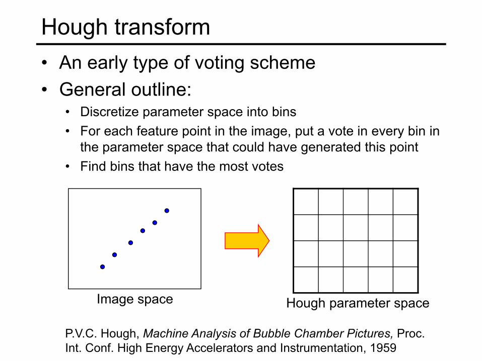
Hough transform• An early type of voting scheme• General outline:

• Discretize parameter space into bins• For each feature point in the image, put a vote in every bin in

the parameter space that could have generated this point• Find bins that have the most votes

P.V.C. Hough, Machine Analysis of Bubble Chamber Pictures, Proc. Int. Conf. High Energy Accelerators and Instrumentation, 1959

Image space Hough parameter space

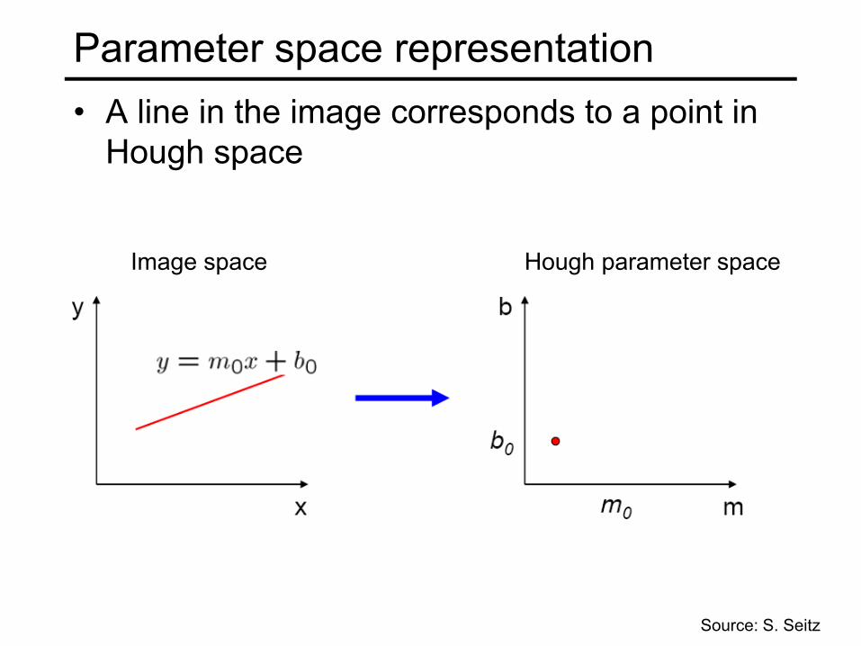
Parameter space representation• A line in the image corresponds to a point in

Hough space

Image space Hough parameter space

Source: S. Seitz

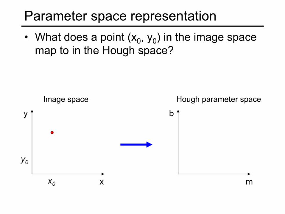
Parameter space representation• What does a point (x0, y0) in the image space

map to in the Hough space?

Image space Hough parameter space

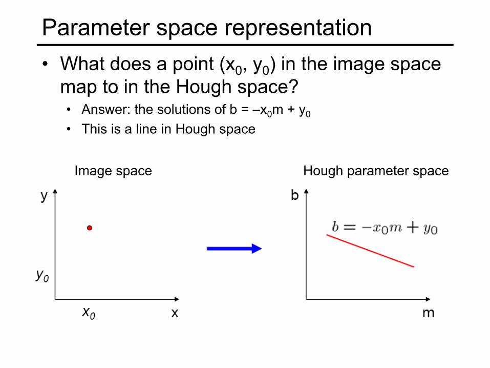
Parameter space representation• What does a point (x0, y0) in the image space

map to in the Hough space?• Answer: the solutions of b = –x0m + y0

• This is a line in Hough space

Image space Hough parameter space

Parameter space representation• Where is the line that contains both (x0, y0)

and (x1, y1)?

Image space Hough parameter space

(x0, y0)

(x1, y1)

b = –x1m + y1

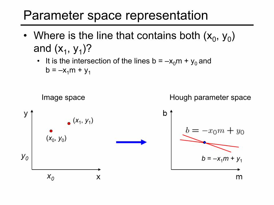
Parameter space representation• Where is the line that contains both (x0, y0)

and (x1, y1)?• It is the intersection of the lines b = –x0m + y0 and

b = –x1m + y1

Image space Hough parameter space

(x0, y0)

(x1, y1)

b = –x1m + y1

• Problems with the (m,b) space:• Unbounded parameter domain• Vertical lines require infinite m

Parameter space representation

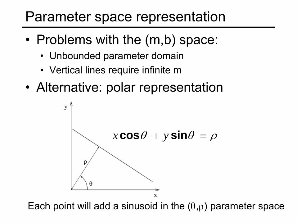
• Problems with the (m,b) space:• Unbounded parameter domain• Vertical lines require infinite m

• Alternative: polar representation

Parameter space representation

ρθθ = + sincos yx

Each point will add a sinusoid in the (θ,ρ) parameter space

Algorithm outline• Initialize accumulator H

to all zeros• For each edge point (x,y)

in the imageFor θ = 0 to 180ρ = x cos θ + y sin θH(θ, ρ) = H(θ, ρ) + 1

endend

• Find the value(s) of (θ, ρ) where H(θ, ρ) is a local maximum

• The detected line in the image is given by ρ = x cos θ + y sin θ

ρ

θ

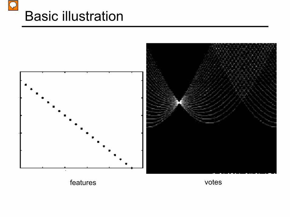
features votes

Basic illustration

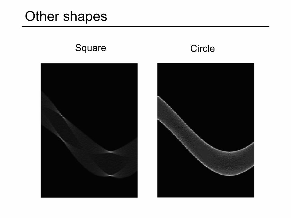
Square Circle

Other shapes

Several lines

features votes

Effect of noise

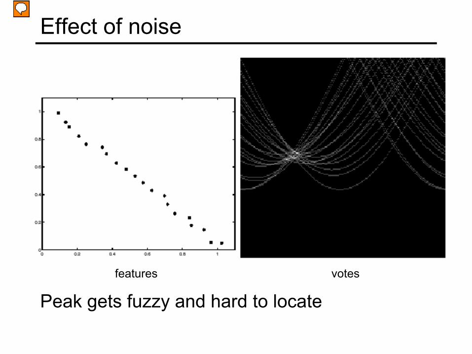
features votes

Effect of noise

Peak gets fuzzy and hard to locate

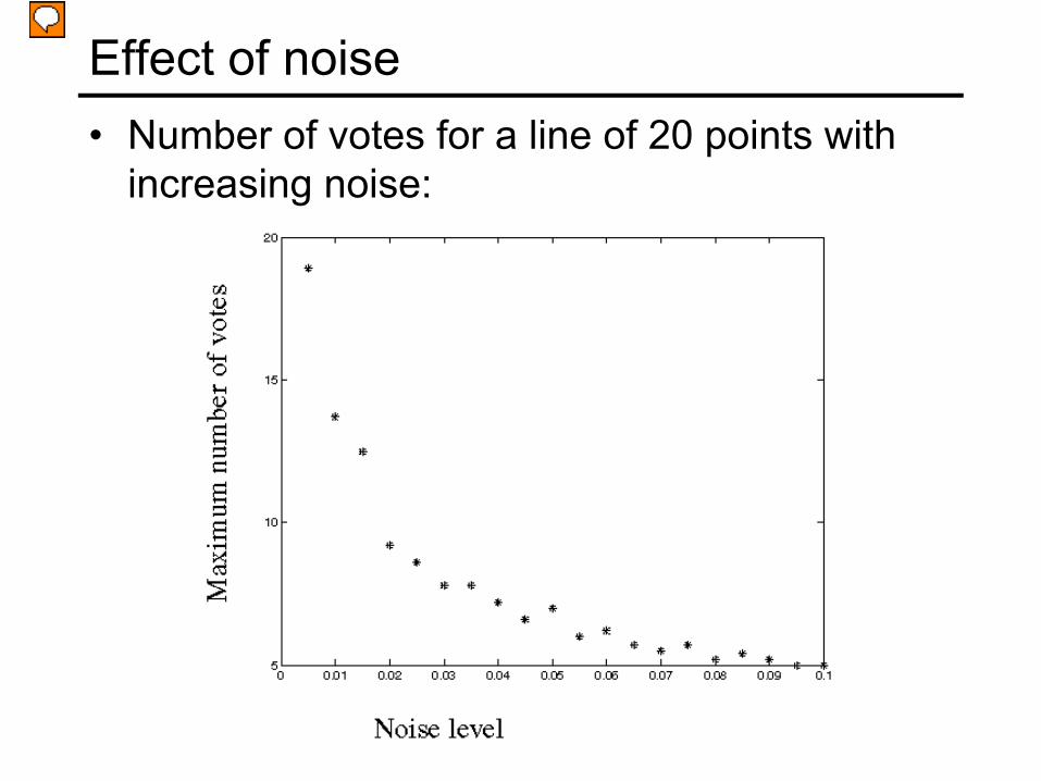
Effect of noise• Number of votes for a line of 20 points with

increasing noise:

Random points

Uniform noise can lead to spurious peaks in the arrayfeatures votes

Random points• As the level of uniform noise increases, the

maximum number of votes increases too:

Practical details• Try to get rid of irrelevant features

• Take only edge points with significant gradient magnitude

• Choose a good grid / discretization• Too coarse: large votes obtained when too many different

lines correspond to a single bucket• Too fine: miss lines because some points that are not

exactly collinear cast votes for different buckets

• Increment neighboring bins (smoothing in accumulator array)

• Who belongs to which line?• Tag the votes

Hough transform: Pros• Can deal with non-locality and occlusion• Can detect multiple instances of a model in a

single pass• Some robustness to noise: noise points

unlikely to contribute consistently to any single bin

Hough transform: Cons• Complexity of search time increases

exponentially with the number of model parameters

• Non-target shapes can produce spurious peaks in parameter space

• It’s hard to pick a good grid size

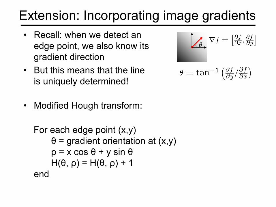
Extension: Incorporating image gradients• Recall: when we detect an

edge point, we also know its gradient direction

• But this means that the line is uniquely determined!

• Modified Hough transform:

For each edge point (x,y) θ = gradient orientation at (x,y)ρ = x cos θ + y sin θH(θ, ρ) = H(θ, ρ) + 1

end

Extension: Cascaded Hough transform• Let’s go back to the original (m,b) parametrization• A line in the image maps to a pencil of lines in the

Hough space• What do we get with parallel lines or a pencil of lines?

• Collinear peaks in the Hough space!

• So we can apply a Hough transform to the output of the first Hough transform to find vanishing points

• Issue: dealing with unbounded parameter space

T. Tuytelaars, M. Proesmans, L. Van Gool "The cascaded Hough transform," ICIP, vol. II, pp. 736-739, 1997.

Cascaded Hough transform

T. Tuytelaars, M. Proesmans, L. Van Gool "The cascaded Hough transform," ICIP, vol. II, pp. 736-739, 1997.

Hough transform for circles• How many dimensions will the parameter

space have?• Given an oriented edge point, what are all

possible bins that it can vote for?

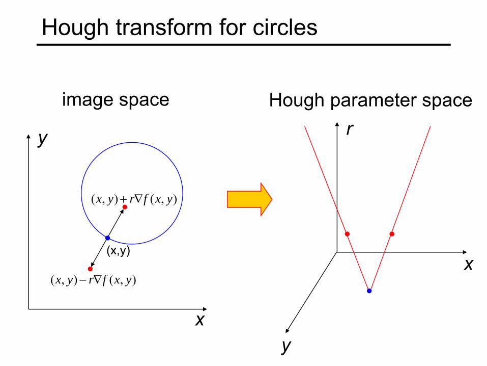
Hough transform for circles

),(),( yxfryx ∇+

x

y

(x,y)x

y

r

),(),( yxfryx ∇−

image space Hough parameter space

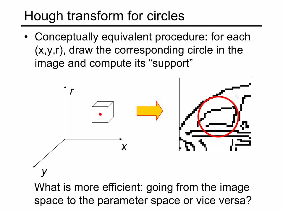
Hough transform for circles• Conceptually equivalent procedure: for each

(x,y,r), draw the corresponding circle in the image and compute its “support”

x

y

r

What is more efficient: going from the imagespace to the parameter space or vice versa?

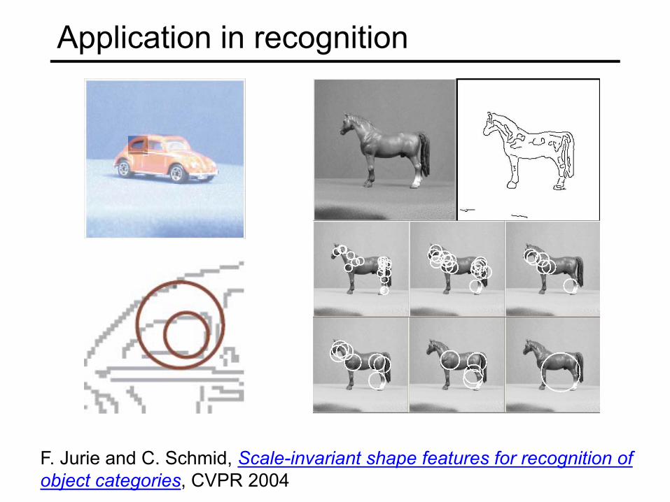
Application in recognition

F. Jurie and C. Schmid, Scale-invariant shape features for recognition of object categories, CVPR 2004

Hough circles vs. Laplacian blobs

F. Jurie and C. Schmid, Scale-invariant shape features for recognition of object categories, CVPR 2004

Original images

Laplacian circles

Hough-like circles

Robustness to scale and clutter

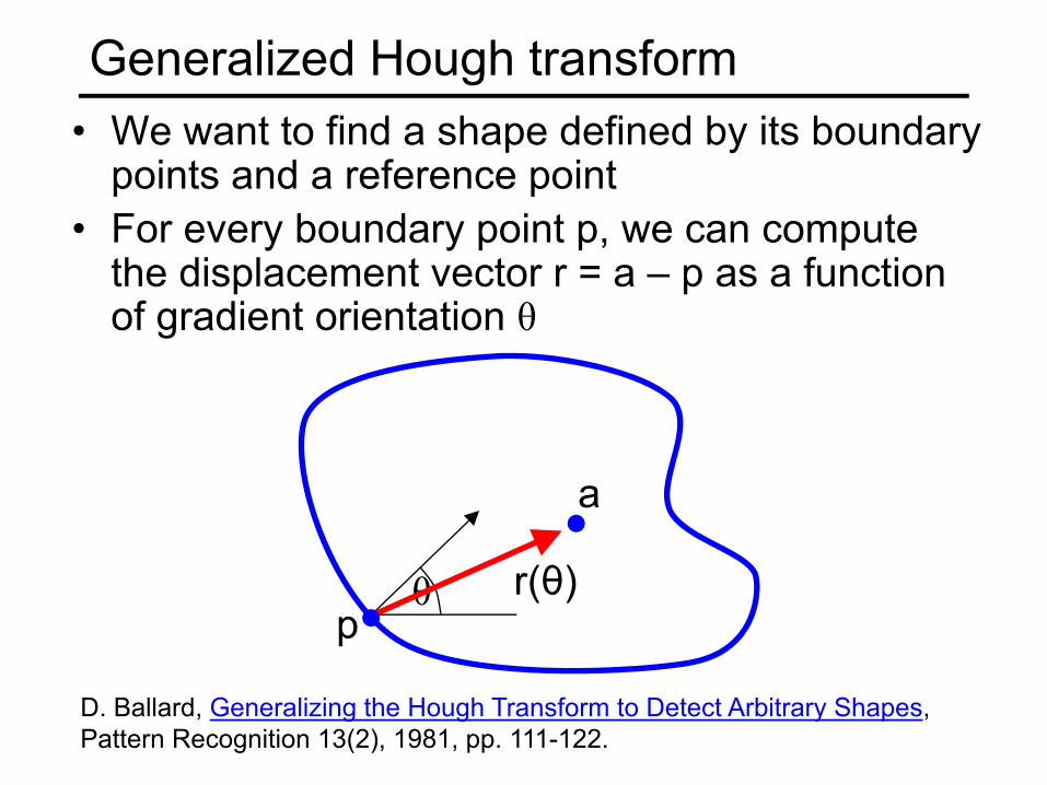
Generalized Hough transform• We want to find a shape defined by its boundary

points and a reference point

D. Ballard, Generalizing the Hough Transform to Detect Arbitrary Shapes, Pattern Recognition 13(2), 1981, pp. 111-122.

a

p

Generalized Hough transform• We want to find a shape defined by its boundary

points and a reference point• For every boundary point p, we can compute

the displacement vector r = a – p as a function of gradient orientation θ

D. Ballard, Generalizing the Hough Transform to Detect Arbitrary Shapes, Pattern Recognition 13(2), 1981, pp. 111-122.

a

θ r(θ)

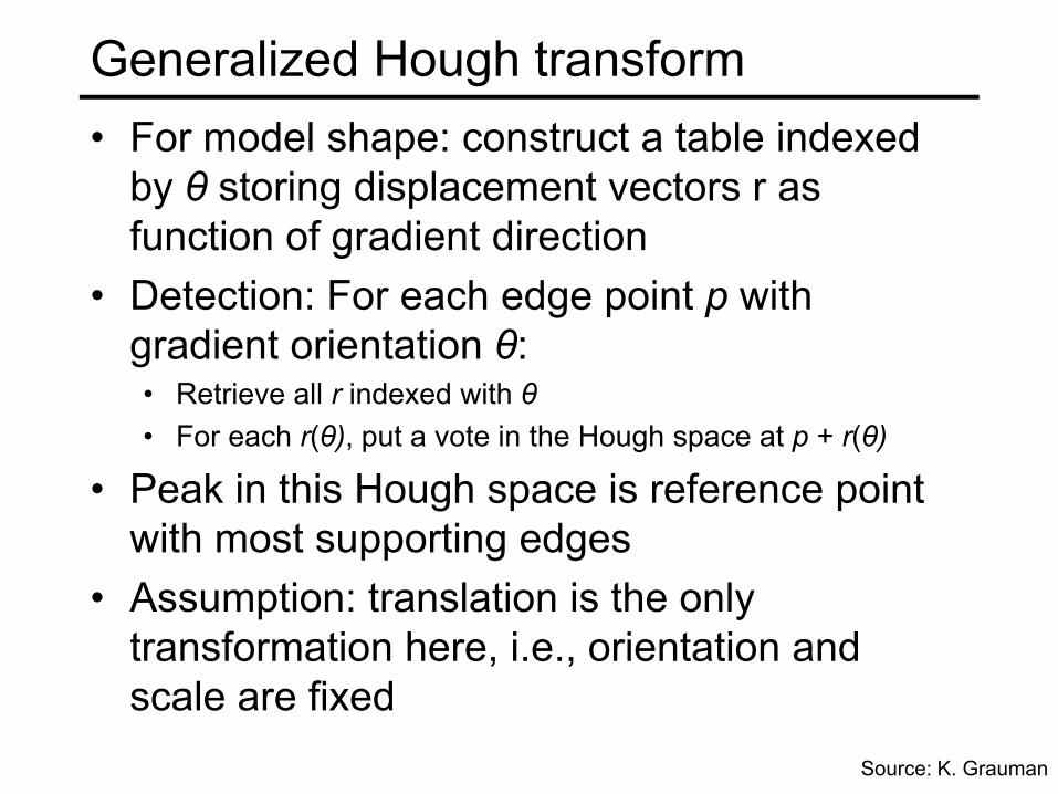
Generalized Hough transform• For model shape: construct a table indexed

by θ storing displacement vectors r as function of gradient direction

• Detection: For each edge point p with gradient orientation θ:• Retrieve all r indexed with θ• For each r(θ), put a vote in the Hough space at p + r(θ)

• Peak in this Hough space is reference point with most supporting edges

• Assumption: translation is the only transformation here, i.e., orientation and scale are fixed

Source: K. Grauman

Example

model shape

Example

displacement vectors for model points

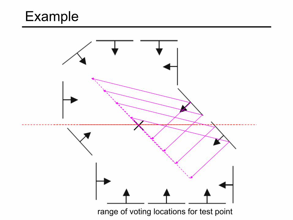
Example

range of voting locations for test point

Example

range of voting locations for test point

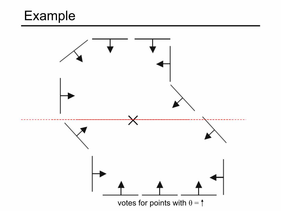
Example

votes for points with θ =

Example

displacement vectors for model points

Example

range of voting locations for test point

votes for points with θ =

Example

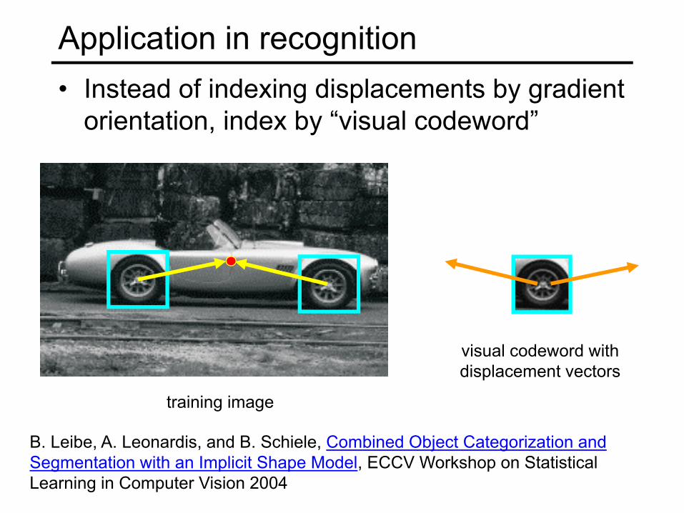
Application in recognition• Instead of indexing displacements by gradient

orientation, index by “visual codeword”

B. Leibe, A. Leonardis, and B. Schiele, Combined Object Categorization and Segmentation with an Implicit Shape Model, ECCV Workshop on Statistical Learning in Computer Vision 2004

training image

visual codeword withdisplacement vectors

Application in recognition• Instead of indexing displacements by gradient

orientation, index by “visual codeword”

B. Leibe, A. Leonardis, and B. Schiele, Combined Object Categorization and Segmentation with an Implicit Shape Model, ECCV Workshop on Statistical Learning in Computer Vision 2004

test image

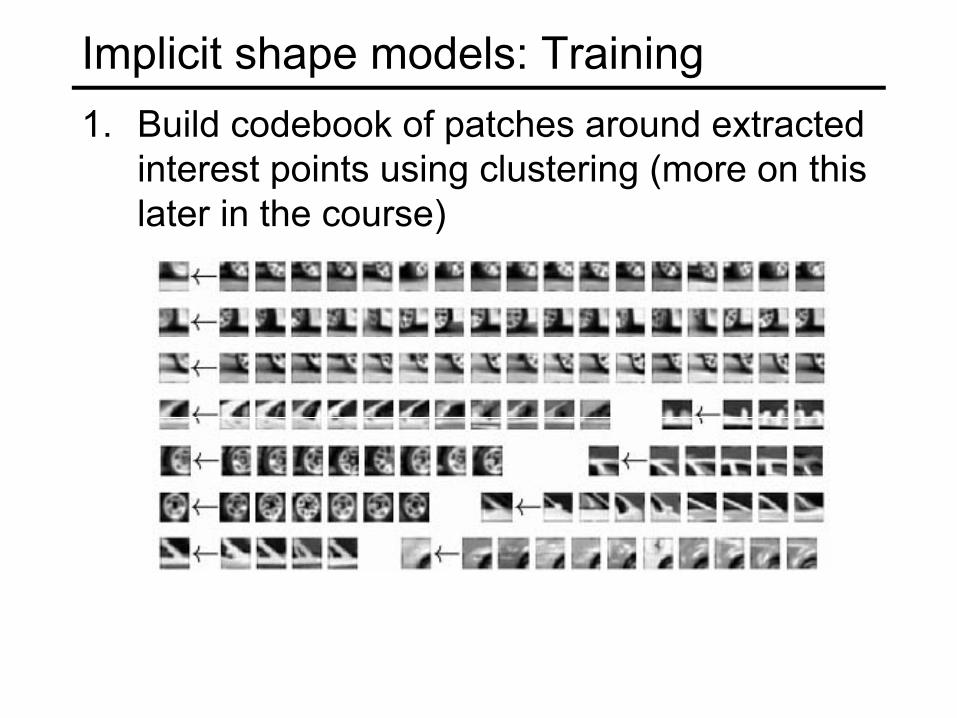
Implicit shape models: Training1. Build codebook of patches around extracted

interest points using clustering (more on this later in the course)

Implicit shape models: Training1. Build codebook of patches around extracted

interest points using clustering2. Map the patch around each interest point to

closest codebook entry

Implicit shape models: Training1. Build codebook of patches around extracted

interest points using clustering2. Map the patch around each interest point to

closest codebook entry3. For each codebook entry, store all positions

it was found, relative to object center

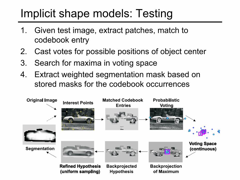
Implicit shape models: Testing1. Given test image, extract patches, match to

codebook entry 2. Cast votes for possible positions of object center3. Search for maxima in voting space4. Extract weighted segmentation mask based on

stored masks for the codebook occurrences

Implicit shape models: Details• Supervised training

• Need reference location and segmentation mask for each training car

• Voting space is continuous, not discrete• Clustering algorithm needed to find maxima

• How about dealing with scale changes?• Option 1: search a range of scales, as in Hough transform

for circles• Option 2: use scale-covariant interest points

• Verification stage is very important• Once we have a location hypothesis, we can overlay a more

detailed template over the image and compare pixel-by-pixel, transfer segmentation masks, etc.