FITTING SPATIAL MODELS OF GEOMETRIC DEVIATIONS OF FREE

Metrol. Meas. Syst., Vol. XVII (2010), No. 4, pp. 599–610

_____________________________________________________________________________________________________________________________________________________________________________________

Article history: received on Aug. 19, 2010; accepted on Oct. 25, 2010; available online on Nov. 26, 2010.

METROLOGY AND MEASUREMENT SYSTEMS

Index 330930, ISSN 0860-8229 www.metrology.pg.gda.pl

FITTING SPATIAL MODELS OF GEOMETRIC DEVIATIONS OF FREE-FORM SURFACES DETERMINED IN COORDINATE MEASUREMENTS Małgorzata Poniatowska, Andrzej Werner Bialystok University of Technology, Division of Production Engineering, Wiejska 45C, 15-351 Bialystok, Poland (� [email protected], +48 85 746 9261, [email protected] )

Abstract

Local geometric deviations of free-form surfaces are determined as normal deviations of measurement points from the nominal surface. Different sources of errors in the manufacturing process result in deviations of different character, deterministic and random. The different nature of geometric deviations may be the basis for decomposing the random and deterministic components in order to compute deterministic geometric deviations and further to introduce corrections to the processing program. Local geometric deviations constitute a spatial process. The article suggests applying the methods of spatial statistics to research on geometric deviations of free-form surfaces in order to test the existence of spatial autocorrelation. Identifying spatial correlation of measurement data proves the existence of a systematic, repetitive processing error. In such a case, the spatial modelling methods may be applied to fitting a surface regression model representing the deterministic deviations. The first step in model diagnosing is to examine the model residuals for the probability distribution and then the existence of spatial autocorrelation.

Keywords: geometric deviations, free-form surface, coordinate measurements, spatial modelling, spatial autocorrelation.

© 2010 Polish Academy of Sciences. All rights reserved

1. Introduction

Machine parts composed of free-form 3D surfaces are more and more often designed. In

designing, producing and measuring such surfaces, CAD/CAM techniques are applied. The accuracy inspection consists in digitalizing the workpiece under research, followed by comparing the obtained coordinates of the measurement points with the CAD design (model) [1, 2]. There are generally two types of measurement data acquisition methods: contact measurement using a coordinate measuring machine (CMM) and non-contact measurement by using an optical/laser scanner. Numerically-controlled CMMs equipped with a ball-end touch trigger or scanning probes, are mainly used for workpiece validation in manufacturing. As a result of the measurement, a set of discrete data is obtained in the form of the coordinates of the measurement points. The values of geometric deviations of the free-form surface, or normal deviations of measurement points from the nominal surface, are performed automatically in software of coordinate measurement machines for each measurement point in the UV scanning option.

Measurements of real surfaces produce only their approximate views. The approximation degree depends on the accuracy of the applied measuring method. Among numerous factors, which have influence on the accuracy, connected with the tool and the measurement environment, there are factors which can be rationally adjusted – such measurement parameters as the sampling interval and the diameter of the measuring tip. Both these factors have a strictly specific impact on the range of information included in measurement data,

M. Poniatowska, A. Werner: FITTING SPATIAL MODELS OF GEOMETRIC DEVIATIONS OF FREE-FORM SURFACES …

determine the least boundary length of elementary irregularities represented in measurement data, because they cause a geometric-mechanical filtration of surface irregularities. The parameter which has a decisive influence is the one which causes a longer wave to be passed. Literature sources suggest different principles of selecting the appropriate tip radius in relation to the sampling interval, most often in the ratios of 1:2, 1:1 and 2:1 [3, 4, 5].

Contact measurements take into consideration deviations of specific wavelengths, which have not been filtered by the ball tip because the ball tip functions as a mechanical-geometrical low-pass filter. Thus, the scope of information included in measurement data depends on the ball tip diameter. In measurement planning, the choice of the diameter d of the ball tip should be made first, according to the measurement purpose and the range of information required on the characteristics of the measured surface [4]. Adopting for measurement the principle suggested in the literature sources pertaining to measuring roundness deviations [3, 6], which states that the boundary wavelength is comparable to the tip radius value, means that in the case of using a stylus tip of d = 1 mm in diameter, irregularities of the length values greater than 0.5 mm are passed; in the case of a stylus tip of d = 2 mm in diameter, irregularities of the length values greater than 1 mm are passed, etc. The second important factor which influences measurement results is the sampling interval T, in the case of scanning a free-form surface with a CMM along a regular grid, which is directly connected to the number of measurement points. In choosing the sampling interval, the principles used in tests on measurement signals, derived from Nyquist theory should be taken into account [7]. The theorem connected with this theory states that the sampling frequency, which is defined as the reciprocal of the sampling interval T, needs to be at least twice as high as the spectrum limit frequency. This particular measurement parameter also results in a mechanical-geometrical filtration, adopting the interval value of 1 mm means that the obtained measurement data contain information of elementary surface irregularities of more than 2 mm in length. Adopting the principles cited in literature [3, 8] to the selection of parameters of contact measurement, at the same time d:T equal to 2:1, choosing a ball of e.g. 2 mm in diameter, and the 1 mm sampling interval, the boundary length of elementary irregularities represented in measurement data amounts to 2 mm.

Geometric deviations of surfaces are attributed to many phenomena that occur during machining, both deterministic and random in character. These phenomena with their consequent machining errors can be described in the space domain. In coordinate measurements of free-form surfaces, spatial data is obtained which provides information on the processing and on geometric deviations in the spatial aspect. Deterministic deviations are spatially correlated, however lack of spatial correlation indicates their spatial randomness. Calculating solely the values of geometric deviations does not provide much information, neither with regard to the surface properties nor to the course of the machining process. Deviations of random values may be spatially correlated which is reflected in their deterministic distribution on a surface and is indicative of the existence of a systematic source in the course of processing. The different nature of geometric deviations may be the basis for decomposing the random and deterministic components [9]. Information concerning deterministic deviations might be used for diagnosing the course of objects processing and subsequently for correcting the processing program.

To research on geometric deviations of free-form surfaces, the methods of analyzing spatial data may be applied [9]. These methods make it possible to quantitatively qualify the spatial interdependence of the given data. Identifying spatial autocorrelation of geometric deviations proves the existence of a systematic, repetitive processing error. In such a case, the theoretical spatial modelling methods [10, 11] may be applied to fitting a surface regression model representing the deterministic deviations. In engineering practice advanced CAD software may be applied for surface modelling. In the article the patch surface interpolation

600


and the shape modification were performed with the use of Rhinoceros software, which is a geometric modeller based on the NURBS method [12, 13]. The first step in model diagnosing is to examine the model residuals for the probability distribution and the existence of spatial autocorrelation. The computations were made in the R-Gui program, which is a software environment for statistical computing and graphics. The described tests were carried out on a free-form surface obtained in the milling process. 2. Measuring spatial autocorrelation

Spatial autocorrelation refers to systematic spatial changes. In general, positive

autocorrelation means that the observed feature values in a selected area are more similar to the features of the contiguous areas than it would result from the random distribution of these values. In the case of negative spatial autocorrelation, the values in the contiguous areas are more different than it would result from their random distribution. Lack of spatial autocorrelation means spatial randomness.

In order to test the existence of spatial dependence, Moran’s statistic for a given variable is applied; it can be used to analyzing spatial data of both normal and unknown probability distribution [10, 11]. The spatial effects range may be researched by means of analyzing the structure of spatial dependence – by testing and selecting weighting matrices defined according to different criteria. Structure of weights is described in [10, 11].

To research on geometric deviations ε (and model residuals e), the following need to be

determined [9]: iε – geometric deviation at each measurement point, ε – arithmetic mean of

geometric deviations at n – measurement points, cij – weighting coefficients, elements of weighting matrices reflecting spatial relations between iε and jε .

A spatial weighting matrix defines the structure of the spatial neighbourhood. The matrix measures spatial connections and is constructed in order to specify spatial dependence. One of the possible dependence structures is assumed, e.g. neighbourhood along a common border, neighbourhood within the adopted radius or within the inverse of distance. In research on geometric deviations, it is most suitable to make the spatial interrelations dependent on the distance between the measurement points, in particular on the inverse of the minimum straight-line distance.

As a result of scanning, the coordinates of the points distributed on the surface along a regular uxv grid are obtained. The distance between the i-th and j-th point, according to the Euclidean metric, is as follows:

( ) ( )2 2

,ij i j i jd x x y y= − + − (1)

where: − xi, yi – i-th point coordinates; − xj, yj – j-th point coordinates; − dij – distance between the i-th and j-th measurement point.

If it is assumed that the dependence between the data values at the i and j points decreases when the distance increases, this relation can be described in the following way:

,fij ijc d −= (2)

where: − cij = 0 for i = j; − f – constant (f ≥ 1).

The spatial autocorrelation coefficient has the following form:

601


( )( )( )∑

∑ ∑

=

= =

−

−−=

n

ii

n

ij

n

jiijc

S

nI

1

2

1 1

0 εε

εεεε, (3)

where: ∑ ∑= =

=n

i

n

jijcS

1 10 ( )ji ≠ ,

− iε – geometric deviation at the measurement point;

− ε – arithmetic mean of geometric deviations at n – measurement points. While examining residuals of a model, the εi geometric deviation values in the (3)

dependency should be replaced with the values of the model residuals ei at these points. After having determined the coefficient I, the null hypothesis of no spatial autocorrelation

at the assumed significance level needs to be verified, examples were shown in [11]. The distribution moments can be determined both at the assumption that the data come from the normal distribution population and at the assumption that they come from the population of an unknown probability distribution. When the number of localities is large, it is reasonable to use the normal approximation. Assuming a normal probability distribution for geometric deviations, the expected value E(I) and the variance var (I) are calculated using the appropriate formulae from [10, 14]. Verifying the hypothesis of no spatial autocorrelation in the data set under research, the test statistics ( ) ( )IIEIz p var/−= needs to be determined, Ip

– the coefficient evaluated from the experimental sample (Eq. (3)), and compared with the limit zα value for the adopted significance level [14]. If z < zα, there is no reason for rejecting the null hypothesis, and in that case the null hypothesis is accepted. In tests on geometric deviations, accepting the null hypothesis means that the tested deviation set is spatially random.

3. Spatial modelling

In order to create a surface model representing deterministic deviations of the surface, the

NURBS method was applied. The NURBS surface of the p degree in the u direction and the q degree in the v direction is a vector function of two variables in the form of [15, 16]:

∑ ∑

∑ ∑

= =

= ==n

i

m

jqjpiji

n

i

m

jjiqjpiji

vNuNw

PvNuNwvuS

0 0,,,

0 0,,,,

)()(

)()(),( . (4)

Points Pi,j make up a two-direction control points grid (Fig. 1) on which the surface patch is lofted (n, m are the numbers of control points in the u and v directions respectively), wi,j are the weights, while Ni,p(u) and Nj,q(v) are the B-spline basis functions defined on knot vectors in the form of:

{

=+

−−++ 1

11

1

1,...,1,,...,,0,...,0p

prp

p

uuU321

, (5)

{

=+

−−++ 1

11

1

1,...,1,,...,,0,...,0q

qsq

q

vvV321

, (6)

where: r = n+p+1 and s = m+q+1.

602


Fig. 1. A NURBS surface patch.

The input data in surface interpolation is a set of points qk,s,(k = 0, ..., r, s = 0, ..., t), forming a spatial grid of (r+1)×(t+1) points. In the case under concern, the data were obtained from coordinate measurements during which a two-direction grid of measurement points was obtained (Fig. 2a).

Fig. 2. Surface approximation: a) grid of approximated points; b) isoparametric curves; c) surface patch.

In developing the geometric model, the method of global surface approximation was used.

The process is carried out in two stages [13, 17]: – in the first stage, a series of curves located on the surface patch (isoparametric curves) are

created. These curves are approximated on the subsequent rows of the pre-set points of one of the parameterization directions, u or v. A spatial grid of control points is obtained this way, with the points defining the isoparametric curves described above (Fig. 2b);

– in the second stage, coordinates of surface control points are determined. It is performed by approximating curves through the control points of the curves which were approximated earlier. The approximation is made in the other parameterization direction. The surface is lofted on the series of curves, which was determined earlier. The obtained control points define unambiguously the surface patch (Fig. 2c). After the approximation stage was completed, shape modification iteration of the created

surface patch was applied in the subsequent stages. These operations aimed at obtaining an adequate model of the regression surface, which would represent deterministic deviations. The model adequacy was tested with the use of methods of analyzing spatial data in research on spatial autocorrelation of the model residuals. The residuals of an adequate model, determined at measurement points, formed a set of random local deviations. In this case, popular procedures were applied of changing the NURBS surface shape, namely [12, 18]: – rebuilding the knot vectors, which influences a change in the number of control points in

the u and v directions); – changing the degrees of B-spline base functions.

603


Fig. 3. Curve shape modification through rebuilding the knot vector: a) 35 control points, 31 internal knots; b) 20 control points, 16 internal knots; c) 15 control points, 11 internal knots.

The effects of changing the shape of the modelled curve with the use of the process of

rebuilding the knot vector are illustrated in Fig. 3. In the first case (Fig. 3a), the curve goes exactly through all the pre-set points (interpolation of the 3rd-degree curve through 33 points). Reducing the number of knots results in reducing the number of control points of the curve. A less-complex shape can be obtained this way (Figs 3b and 3c). The surface shape modification is performed according to the same rules which are applied to change the shape of the curve. 4. Experimental investigations

The experiments were performed on a free-form surface of a workpiece made of

aluminium alloy with the base measuring 50 x 50 mm (Fig. 4), obtained in the milling process using a ball-end mill 6 mm in diameter, rotational speed equal to 7500 rev/min, working feed 300 mm/min and zig-zag cutting path in the XY plane. The measurements were carried out under laboratory conditions on Global Performance CMM (PC-DMIS software, MPEE = 1.5 + L/333 µm, equipped with a Renishaw SP25M probe, 20 mm stylus with ball tips of 2 mm and 4 mm in diameter).

Fig. 4. CAD model of the surface.

The surface was scanned in two stages (without applying radius compensation) with the UV scanning option (the option built in PC-DMIS software). In the first stage 2500 uniformly distributed measurement points were scanned from the surface (50 rows x 50 columns) with the use of a ball end tip of 2 mm in diameter. In the second stage 625 points were scanned (25

604


-0,04-0,03

-0,02-0,01

0,00

0,01

10

20

3040

10

20

30

40

ε [m

m]

X [mm]

Y [mm]

-0,04 -0,03 -0,02 -0,01 0,00 0,01

Histogram

-0,036 -0,025 -0,014 -0,003 0,007

ε [mm]

0

100

200

300

400

500

600

num

b. o

bs.

rows x 25 columns) using a ball tip of 4 mm in diameter. In both cases the process of fitting the data to the nominal surface was then carried out in which the least square method was applied and all the measurement points were used; the measurement process was subsequently repeated and geometric deviations ε were computed [19]. In this way the position deviations were minimized. All the measurements were repeated tree times; the tables and plots present mean values of the obtained results.

The amount of information included in measurement data depends on the ball tip diameter and sampling interval (grid size). Both these factors cause in fact a geometrical-mechanical filtration of surface irregularities (Section 1). In the first case the observed data include information on surface geometric deviations of the lengths exceeding 2 mm, in the second case – deviations of lengths exceeding 4 mm. 4.1. Measurement results

The obtained measurement data are presented in a graphical form. Fig. 5a shows a spatial

plot of the ε deviations with reference to the x and y nominal coordinates and Fig. 5b the probability plot of deviations for 2500 measurement points. Fig. 6 shows the maps of deviations for both cases. The statistical parameters of ε sets are compiled in Table 1.

a) b)

Fig. 5. Plots of geometric deviations for 2500 measurement points: a) spatial plot versus the XY plane; b) probability distribution.

Table 1. Statistical parameters of (ε) geometric deviation sets.

Number of meas. pts. 2 500 625 Sampling grid 0.01ux0.01v 0.02ux0.02v Sampling interval T [mm] ~ 1 mm ~ 2 mm Tip diameter d [mm] 2 4 Std. deviation [mm] 0.011 0.009 Mean [mm] -0.012 -0.010 Minimum ε [mm] -0.037 -0.035 Maximum ε [mm] 0.020 0.013 Form/waviness dev. [mm] 0. 057 0.048

The deviation plots indicate that the measurement points contain both the deterministic and

the random component and that the contribution of the deterministic component is greater (Fig. 5, Fig. 6). Comparing the maps for different sampling parameters, significant differences

605


in irregularity shapes and the numbers of observed details can be seen. The values of the observed shape/waviness deviations also vary among each other (Table 1).

Fig. 6. Maps of geometric deviations: for 2500 measurement points (left) and for 625 measurement points (right).

For the tip end of d = 2 mm in diameter, the mean and minimum values of the observed

local geometrical deviations were smaller. This tip went deep into the surface irregularities and reached surface points which were located lower than the points established with the use of the tip end of d = 4 mm. Moreover, the scatter of the values of the observed deviations was greater. The form/waviness deviation determined in measurements with the use of the tip end of d = 2 mm was greater by approx. 0.009 mm.

For both data sets tests on spatial autocorrelation of geometric deviations were subsequently carried out [9]. The relationships between the deviations were made dependent on the reciprocal distances determined from the formula (2). The elements of weight matrices defining the dependencies between deviations at points i and j were calculated from formula (2) assuming the value of the constant as f = 3. A fragment of the weight matrix is shown in Fig. 7a. The spatial autocorrelation coefficient I was determined and the null hypothesis on the lack of geometric deviations autocorrelation was verified, assuming a randomized probability distribution, with the significance level α = 0.01 (the upper point of a standard normal distribution zα = 2.34). The computations were performed in the R-Gui program. Fig. 7b presents the print screen image with the computation results for the case of 2500 measurement points.

a) b)

Fig. 7. a) The top left corner of the W matrix. b) Print screen image with computation results.

X [mm]

10 20 30 40

Y [m

m]

10

20

30

40

-0,04 -0,03 -0,02 -0,01 0,00 0,01 X [mm]

10 20 30 40Y

[mm

]

10

20

30

40

-0,04 -0,03 -0,02 -0,01 0,00 0,01

606


The null hypothesis of the lack of spatial autocorrelation was rejected, I = 0.84; z = 77.69; zα = 2.34; z > zα. The computation results show a clear positive autocorrelation of local geometrical deviations, as well as the results for 625 measurement points. In both cases it is possible to predict the values in the neighbouring points on the basis of the deviation value at any point.

The test results indicate the existence of systematic processing errors. Further, the spatial model of deterministic geometric deviations needs to be determined and their sources of influence minimized, and/or the processing program needs to be corrected.

4.2. Fitting models of geometric deviations

In both cases the regression surfaces which represent deterministic deviations, were modelled. In the subsequently constructed models, the number of control points and the surface degrees in both directions (Section 3). The model residuals were examined each time, and the maximum and minimum values, arithmetic mean (should be ~ 0), probability distribution (the distribution normality was verified with the Kolmogorov-Smirnov test), and the I spatial autocorrelation coefficient (3) were determined. In all statistical tests a confidence level P = 0.99 was adopted. The model with the smallest number of control points and the lowest surface degrees in the X and Y directions, for which the model residuals met the criteria of a normal distribution and of spatial randomness, was adopted as an adequate one. In the case of 2500 measurement points, the criterion was met for the number of control points amounting to 31x31, the number of surface degrees being 3x3. In the case of 625 measurement points, the criterion was met for the number of control points amounting to 16x16. Fig. 8 presents the probability distributions of model residuals.

a) b)

Fig. 8. Probability distributions of model residuals: a) for 2500 points; b) for 625 points.

Table 2. Modelling and computation results.

Number of meas. pts. 2500 625 Control points number of deterministic surface

31x31 16x16

Surface degrees 3x3 3x3 Deterministic deviations [mm] -0.035 ÷ +0.012 -0.035 ÷ +0.010 Autocorrelation coefficient I for model residuals

0.04 0.04

Test statistics z for model residuals

2.21 1.86

Random deviations e [mm] -0.008 ÷ +0.006 -0.010 ÷ +0.013 Mean of random dev. e [mm] 0.000 0.000

HistogramK-S d=,031

-0,008-0,006

-0,004-0,002

0,0000,002

0,0040,006

e [mm]

0

100

200

300

400

500

num

b ob

s.

HistogramK-S d=,090

-0,009-0,006

-0,0030,000

0,0030,006

0,0090,012

e [mm]

0

50

100

150

200

250

num

b. o

bs.

607


The spatial autocorrelation coefficients I for model residuals were determined, and the null hypotheses on the lack of geometric deviations autocorrelation were verified, assuming a normal probability distribution, with the significance level α = 0.01. The computation and modelling results for both cases are compiled in Table 2. The computation results show a lack of spatial autocorrelation of model residuals. The determined models represent deterministic deviations, whereas the residuals of the models constitute the random deviations.

a) b)

Fig. 9. Maps of the deterministic deviations: a) for 2500; b) for 625 measurement points.

Fig. 9 presents maps of the deterministic deviations; the maps and spatial plots for the random deviations are shown in Fig. 10 and Fig. 11.

Fig. 10. The map and the spatial model of the random deviations for 2500 measurement points.

X [mm]10 20 30 40

Y [m

m]

10

20

30

40

-0,008 -0,006 -0,004 -0,002 0,000 0,002 0,004 0,006

-0,008-0,006-0,004

-0,0020,000

0,0020,004

0,006

10

20

30

40

10

20

30

40

e [m

m]

X [mm

]

Y [mm]

-0,008 -0,006 -0,004 -0,002 0,000 0,002 0,004 0,006

X [mm]10 20 30 40

Y [m

m]

10

20

30

40

-0,04 -0,03 -0,02 -0,01 0,00 0,01

X [mm]10 20 30 40

Y [m

m]

10

20

30

40

-0,03 -0,02 -0,01 0,00 0,01 0,01

608


X [m m ]10 20 30 40

Y [m

m]

10

20

30

40

-0,010 -0,008 -0,006 -0,004 -0,002 0,000 0,002 0,004 0,006 0,008 0,010 0,012

-0,010-0,008-0,006-0,004-0,0020,0000,0020,0040,0060,0080,0100,012

10

20

30

40

10

20

30

40

e [m

m]

X[mm]

Y [mm]

-0,010 -0,008 -0,006 -0,004 -0,002 0,000 0,002 0,004 0,006 0,008 0,010 0,012

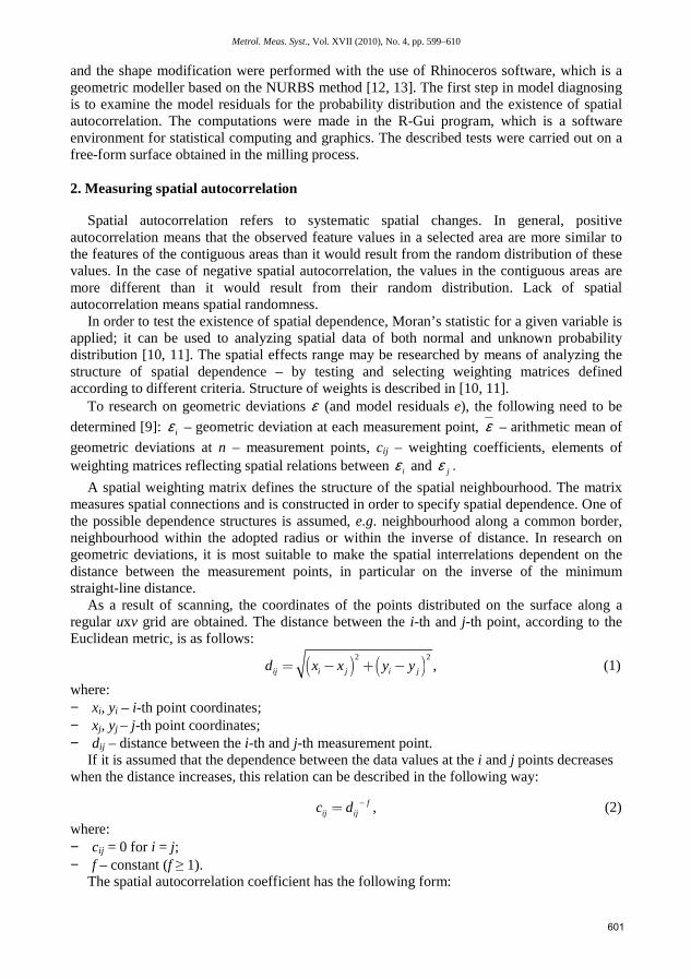
Fig. 11. The map and the spatial model of the random deviations for 625 measurement points.

Observing the maps of the deterministic deviations (Fig. 9), the effect of rejecting random deviations is visible. The surface modelled using 2500 points contains surface irregularities of visibly shorter lengths and is more complex than the surface modelled with 625 points. The value of the deterministic component is greater for the first surface, whereas the random component, i.e. the scatter of model residuals, is smaller for this surface (Fig. 9, Table 2). The complexity of the modelled surfaces depends on the number of control points, connected in fact with the number and distribution of measurement points.

Random deviations (Fig. 10 and Fig. 11) of both cases differ significantly in the lengths of irregularities. This is strictly connected with measurement parameters, the number of measurement points and the ball tip diameter. Different effects of surface irregularity decomposition are clearly visible.

5. Conclusions

On the basis of the results of measuring geometric features of surfaces, it is possible to infer the course of the machining process. The observed geometric deviations are caused by machining inaccuracies. Phenomena of a systematic, deterministic character result in forming geometric deviations of the same character on the object surface. These deviations can be minimized by removing their sources from the process and/or, in the case of numerically controlled machining, by correcting the machining programme, using the data obtained from measurements. Free surfaces are produced with the use of multiaxis machining centres, and most often measured with NC CMMs. Geometric deviations of free-form surfaces, evaluated by coordinate measurements, are of a spatial character, and it is the same with the character of the sources of these deviations in the machining process. The article suggests a method of creating a model of a surface representing determined deviations, applying spatial statistics and geometric spatial modelling. The method consists in iterative modelling of the surface of the determined deviations and in testing the spatial randomness of the model residuals at the consecutive iteration stages. The method makes it possible to reject deviations of a random character from the measurement data set. The obtained surface model might be a basis for correcting the machining programme. The result of modelling depends, among others, on the

609


adopted measurement parameters such as the diameter of the measuring tip, and, above all, the sampling interval (and thus the number of measurement points).

The results of the research carried out with the use of the developed method for the measurement data of a milled surface showed that separate random geometric deviations comprised between ¼ and ½ of the deviations obtained as a result of measurement, depending on the sampling parameters used in measuring.

Acknowledgments

The work is supported by the Polish Ministry of Science and Higher Education under research project No. N N503 326235.

References [1] ElKott, D.F., Veldhuis, S.C. (2007). Cad-based sampling for CMM inspection of models with sculptured

features. Eng. Comp., 23, 187-206.

[2] Obeidat, S.M., Raman, S. (2009). An intelligent sampling method for inspecting free-form surfaces. Int. J. Adv. Manuf. Technol., 40, 1125-1136.

[3] Adamczak, S. (2008). Surface geometric measurements. Warszawa: WNT. (in Polish).

[4] Dong, W.P., Mainsah, E., Stout, K.I. (1996). Determination of appropriate sampling conditions for three-dimensional microtopography measurement. Int. J. Mach. Tools Manuf., 36, 1347-1362.

[5] Pawlus, P. (2004). Mechanical filtration of surface profiles. Measurement, 35, 325-341.

[6] Adamczak, S., Janecki, D., Makieła, W., Stępień, K. (2010). Quantitative comparison of cylindricity profiles measured with different methods using Legendre-Fourier coefficients. Metrol. Meas. Syst., 17(3), 233-244.

[7] Szabatin, J. (2003). Signal theory fundamentals. Warszawa: WKŁ. (in Polish).

[8] Pawlus, P. (2004). Mechanical filtration of surface profiles. Measurement, 35, 325-341.

[9] Poniatowska, M. (2009). Research on spatial interrelations of geometric deviations determined in coordinate measurements of free-form surfaces. Metrol. Meas. Syst., 16(3), 501-510.

[10] Cliff, A.D., Ord, J.K. (1981). Spatial Processes. Models and Applications. London: Pion Ltd.

[11] Kopczewska, K. (2007). Econometrics and Spatial Statistics. Warszawa: CeDeWu. (in Polish).

[12] Hu, S.M., Li, J.F., Ju, T., Zhu, X. (2001). Modifying the shape of NURBS surfaces with geometric constrains. Comp. Aided Des., 33, 903-912.

[13] Wang, W.K., Zhang, H., Park, H., Yong, J.H.,. Paul, J.C, Sun, J.G. (2008). Reducing control points in lofted B-spline surface interpolation using common knot vector determination. Comp. Aided Des., 40, 999-1008.

[14] Upton, G.J.G., Fingleton, B. (1985). Spatial Data Analysis by Example. John Willey & Sons.

[15] Piegl, L., Tiller, W. (1997). The NURBS book. 2nd ed. New York: Springer-Verlag,.

[16] Brujic, D., Ristic, M., Ainsworth, I. (2002). Measurement-based modification of NURBS surfaces. Comp. Aided Des. 34, 173-183.

[17] Hansford, D., Farin, G. (2002). Curve and Surface Constructions. Handbook of Computer Aided Design. Elsevier Science B.V., Amsterdam, 165-192.

[18] Juhász, I., Hoffmann, M. (2004). Constrained shape modification of cubic B-spline curves by means of knots. Comp. Aided Des., 36, 437-445.

[19] Poniatowska, M. (2008). Determining uncertainty of fitting discrete measurement data to a nominal surface. Metrol. Meas. Syst., 15(4), 595-606.

610

Documents

FITTING SPATIAL MODELS OF GEOMETRIC DEVIATIONS OF FREE