Embed Size (px)
Citation preview
ORIGINAL ARTICLE
doi:10.1111/j.1558-5646.2012.01610.x
FISHER’S GEOMETRICAL MODEL OF FITNESSLANDSCAPE AND VARIANCE IN FITNESSWITHIN A CHANGING ENVIRONMENTXu-Sheng Zhang1,2,3
1Institute of Evolutionary Biology, School of Biological Sciences, University of Edinburgh, West Mains Road, Edinburgh
EH9 3JT, United Kingdom2Present address: Statistics, Modeling and Bioinformatics Department, Centre for Infections, Health Protection Agency,
London NW9 5EQ, United Kingdom3E-mail: [email protected]
Received April 6, 2011
Accepted February 6, 2012
Data Archived: Dryad: doi:10.5061/dryad.6r138b0h
The fitness of an individual can be simply defined as the number of its offspring in the next generation. However, it is not
well understood how selection on the phenotype determines fitness. In accordance with Fisher’s fundamental theorem, fitness
should have no or very little genetic variance, whereas empirical data suggest that is not the case. To bridge these knowledge
gaps, we follow Fisher’s geometrical model and assume that fitness is determined by multivariate stabilizing selection toward an
optimum that may vary among generations. We assume random mating, free recombination, additive genes, and uncorrelated
stabilizing selection and mutational effects on traits. In a constant environment, we find that genetic variance in fitness under
mutation-selection balance is a U-shaped function of the number of traits (i.e., of the so-called “organismal complexity”). Because
the variance can be high if the organism is of either low or high complexity, this suggests that complexity has little direct costs.
Under a temporally varying optimum, genetic variance increases relative to a constant optimum and increasingly so when the
mutation rate is small. Therefore, mutation and changing environment together can maintain high genetic variance. These results
therefore lend support to Fisher’s geometric model of a fitness landscape.
KEY WORDS: Adaptation, changing environment, Fisher’s geometrical model, genetic variance in fitness, mutation-selection
balance, multivariate stabilizing selection.
The fitness of an individual can be defined in terms of the num-
ber of its fertile offspring, and is a function of its survival and
reproductive performance. Fitness can be regarded as a quanti-
tative trait, but in natural populations it is difficult to determine
how other traits influence fitness. Although it is clear that in
Drosophila, for example, there is an overt relationship between
female egg production and fitness, the relationship between bris-
tle number and fitness is less obvious. For some traits there is
likely to be a monotonic relationship with fitness, for others it
may be quadratic with an intermediate optimum (Falconer and
Mackay 1996; Walsh and Lynch 2009). How phenotype deter-
mines fitness is one of the fundamental challenges to developing
the evolution theory of adaptation (Stearns and Hoekstra 2000;
Orr 2005; Wagner and Zhang 2011).
Fisher’s (1958) fundamental theorem shows that the rate of
change in fitness is equal to the additive genetic variance in fit-
ness. Thus natural selection would be expected to use up the
useful variance (Crow 2008). However, variation in fitness re-
mains at high levels in populations (Mousseau and Roff 1987;
Merila and Sheldon 1999; Hill and Zhang 2008; Long et al. 2009).
2 3 5 0C© 2012 The Author(s). Evolution C© 2012 The Society for the Study of Evolution.Evolution 66-8: 2350–2368

GENETIC VARIATION IN FITNESS
For example, Fowler et al. (1997) allowed replicated competition
of a sample of wild-type third chromosome of D. melanogaster
against balancer chromosomes in a population cage, and estimated
fitness by recording changes in chromosome frequency. They ob-
tained an estimate of the genetic variance in loge fitness for the
whole genome as high as 0.45. Genetic variation in fitness can
be maintained by mutation and other factors such as heterozygote
superiority and heterogeneous environments; genetic variation in
other traits can remain through these factors and also because
the covariance with fitness may be small (for discussion see, e.g.,
Falconer and Mackay 1996; Lynch and Walsh 1998; Burger 2000;
Zhang and Hill 2005a; Crow 2008). Although there are some theo-
retical models to provide qualitative understanding of why genetic
variance in fitness remains (Charlesworth and Hughes 2000), sat-
isfactorily quantitative models are not available. To understand the
maintenance of genetic variance in fitness, we need a model to
describe how fitness is controlled by mutant genes and genotypes
and how natural selection acts on them.
Fisher (1930) was one of the first to consider this relationship.
He introduced a geometrical model of natural selection acting on
multiple quantitative traits that characterize an individual: each
trait has an environment-dependent optimal value and the fitness
of a complete phenotype is jointly determined by the distances
of the traits from their optimal values. For phenotypes near this
optimum, selection is of stabilizing type while phenotypes far
from it are consequently subject to directional selection (Barton
1998). There is some evidence for stabilizing selection and con-
sequent directional selection on various traits (Kingsolver et al.
2001; Elena and Lenski 2003; Hereford et al. 2004). Although
this selection model appears simplistic, it has been widely applied
to different aspects of evolutionary biology (e.g., Poon and Otto
2000; Orr 2000; Barton 2001; Welch and Waxman 2003; Waxman
and Welch 2005; Martin and Gandon 2010). Importantly, an anal-
ysis of the fitness effects of mutations across environments shows
that predictions from Fisher’s geometrical model are consistent
with empirical estimates, implying that multivariate stabilizing
selection is a reasonable fitness landscape model (Martin and
Lenormand 2006b).
A phenotype can be characterized by a very large number of
traits (Zhang and Hill 2003; Wagner and Zhang 2011). Because
the total number of genes is limited, most genes must affect more
than one trait (i.e., pleiotropy is common) (Barton and Keightley
2002; Mackay 2004; Ostrowski et al. 2005; Weedon and Frayling
2008; Wagner et al. 2008; Wang et al. 2010). Further, environ-
mental constraints on traits are not independent, so selection on
these traits is also expected to be correlated (Welch and Waxman
2003; Zhang and Hill 2003; Blows 2007). The complicated situ-
ation can be reduced, however, by simultaneous diagonalization
of the mutation matrix and the selection matrix (Zhang and Hill
2003; Hine and Blows 2006) such that the number of traits that
are under independent selection and mutationally independent is
much smaller (Waxman and Welch 2005; Hine and Blows 2006;
McGuigan et al. 2011). By comparing theoretical predictions with
empirical data on the distribution of mutational effects on fitness,
Martin and Lenormand (2006a) suggest there could be less than
three independent traits for some model species.
In the discussion of adaptation, it is usual to assume that the
population has suffered a one time environmental change such
that it departs from the current optimum for many generations
(Orr 2005). The question of interest is how often the optimum
changes and what kind of mutation emerges to help the popu-
lation catch up with the changing optimum (Bello and Waxman
2006; Kopp and Hermisson 2007). A large change is rare but small
changes must be frequent. The idea that an environmental change
determines a new phenotypic optimum is supported by the long-
term adaptation of experimental populations to new environments
(for review see Elena and Lenski 2003 for microbes and Gilligan
and Frankham 2003 for Drosophila). By comparing predictions
for a fitness landscape model (Martin and Lenormand 2006a)
and observations from mutation accumulation experiments,
Martin and Lenormand (2006b) concluded that a Gaussian fitness
function with a constant width across environments and with an
environment-dependent optimum is consistent with the observed
patterns of mutation accumulation experiments. As environment
may change randomly or directionally, so does the movement in
the optimum. With changes such as these in the position of the
optimum, the effect of a mutant on fitness varies over genera-
tions even though the mutational effect on quantitative traits may
not (Martin and Lenormand 2006b; cf. Hermisson and Wagner
2004).
Theoretical studies show that stabilizing selection toward a
directionally moving optimum under recurrent mutation is an im-
portant mechanism for maintaining quantitative genetic variation
(Burger 1999; Waxman and Peck 1999; Burger and Gimelfarb
2002). With a directionally moving optimum, mutant alleles suf-
fer both stabilizing and directional selection; mutants become
beneficial if they draw phenotypes toward the moving optimum
and rise in frequency, which then increases the genetic variance.
Previous investigations based on a quadratic fitness function, how-
ever, show that a randomly fluctuating optimum can hardly in-
crease the quantitative genetic variance (Turelli 1988). Based on a
Gaussian fitness function, Burger and Gimelfarb (2002) showed
that stochastic perturbation of a periodic optimum, in combination
with recurrent mutation, can increase genetic variance substan-
tially; but Burger (1999) showed that purely fluctuating selection
cannot increase genetic variance.
In this study we employ Fisher’s (1958) model for the map
between mutational effects on quantitative traits and the fitness ef-
fect with a changing optimum to investigate the variance in fitness
under mutation-selection balance (MSB). Any realistic scenario
EVOLUTION AUGUST 2012 2 3 5 1

XU-SHENG ZHANG
may be complicated, but here we consider an idealized situation
of additive genes, free recombination, and a large population with
random mating. Results from these simplified models should pro-
vide essential and useful information for more complicated and
realistic situations. Moreover, taking into account empirical data
for mutation and selection parameters, we test whether this model
can provide a quantitative interpretation for the high level of ge-
netic variance in fitness. Based on these results, we further discuss
how pleiotropy affects the genetic variance in fitness and the so-
called “cost of complexity” (Orr 2000), and review the validity of
the Fisher geometric model of fitness.
ModelsA population of N diploid monoecious individuals with discrete
generations, random mating and at Hardy–Weinberg equilibrium,
is assumed. The following independent and symmetric assump-
tions are made for mutational effects and selection on quantitative
traits. Each individual is characterized by phenotypes of n inde-
pendent identical quantitative traits z = (z1, z2, . . . , zn)T with T
representing transposition. There is free recombination and addi-
tive gene action within and between loci. Mutations have effects
a = (a1, a2, . . . , an)T on the n traits, with ai being the difference
in value between homozygotes, with their density function f (a)
following a multivariate normal distribution N(0, ε2I). A random-
walk model of mutation is assumed (Crow and Kimura 1963;
Zeng and Cockerham 1993): a mutation of effect a changes the
phenotype of an individual from z to z + a. Here we implicitly as-
sume the so-called Euclidean superposition model, within which
mutational effects on individual traits are independent of the total
number of traits affected and have the same mean (Wagner et al.
2008).
We assume there is no genotype-environment interaction and
the environmental variation in a quantitative trait is N(0, VE).
Thus, by averaging environmental deviations, the phenotype z is
simply represented by its genotype (Turelli 1984). Individuals are
subject to real stabilizing selection, with independent and identical
strength of selection on each trait, characterized by S = ζ2I, where
ζ2 = 1/(2VS) and VS is the variance of the fitness profile on each
trait. Multivariate Gaussian fitness
W (z) ≡ exp(Q) = exp
⎡⎣−1
2
n∑j=1
(z j − o j )2ζ2
j
⎤⎦ (1)
is assigned to genotypic values z, with the optimum phenotype
o = (o1, o2, . . . , on)T, and the loge fitness is defined as
Q ≡ ln (W (z)) = −1
2
n∑j=1
(z j − o j )2ζ2
j . (2)
We consider the following schemes for a moving optimum.
(1) Directionally moving optimum: The optimum, starting from
0, moves at a constant rate κ = (κ, κ, . . . , κ),
Ot = κt, (3)
(cf. Charlesworth 1993; Burger 1999; Waxman and Peck
1999). We employ the standard deviation of environmental
variation in trait (i.e., σE = √V E) as a suitable scale (cf.
Houle 1992).
(2) Gaussian change (i.e., white noise): We assume optimal
values are independent and identical and the optimum for
each trait fluctuates around its overall mean zero with vari-
ance VO. The optimum phenotype ot among traits within
generation is distributed as N(0, VOI).
(3) Markov process: A simple situation where optimal values
for different traits are uncorrelated, but those for the same
trait are autocorrelated among generations. The optimum
follows a linear stationary Markov process, with mean zero,
variance VO,j, and autocorrelation coefficient dj (-1 < dj <
1) between ot,j, t = 0, 1, 2, . . . . for trait j; that is,
O j,t = d j O j,t−1 + δ j,t−1, j = 1, . . . , n (4)
(Charlesworth 1993). Here δj represent white noise with
mean zero and variance Vj, with VO,j = Vj/(1 − dj)2. Only
the symmetric situation is considered, where Vj = V and
dj = d, j = 1, . . . , n.
(4) Periodically moving optimum: To take into account auto-
correlation among optimal values, we consider they change
in a periodic way as
O j,t = A sin(2πt/P), j = 1, . . . , n (5)
with a period of P generations and an amplitude A (cf.
Charlesworth 1993; Burger and Gimelfarb 2002). The op-
timum will have mean zero and variance A2j /2 for trait j. It
changes more regularly than the randomly changing opti-
mum but less so than the directionally moving optimum.
MethodsWe use Monte-Carlo simulations to investigate genetic variances
in quantitative traits and in fitness. For constant and randomly
varying environments, results are also obtained by employing
Kimura’s (1969) diffusion approximation.
DIFFUSION APPROXIMATION
Let the frequencies of the wild-type allele (A) and the mutant
allele (a) at locus i be 1 − xi and xi, respectively, the frequencies of
genotypes AA, Aa, and aa assuming Hardy–Weinberg proportions
are (1 − xi)2, 2xi(1 − xi), and xi2. With additive gene action, the
2 3 5 2 EVOLUTION AUGUST 2012
GENETIC VARIATION IN FITNESS
genotypic values for the quantitative trait j are 0, 12 ai,j, and ai,j.
Summing over all loci, the genetic variance in quantitative trait j
can be written as
VG, j (T) =∑
i
H (si )a2i, j/4 j = 1, . . . , n. (6)
Here H(si) = 2xi(1 − xi) is the heterozygosity at locus i and
the frequency xi is determined by the selective value si ≡W(z+ai)/W(z) − 1 for the mutation with effects ai. With a fixed
optimum, the mean phenotype is coincident with the optimum
(Burger 2000) and the selective value of mutant allele i can be
approximated by
si ≈ Qi = −1
2
n∑j=1
a2i, j ζ
2 (7)
(Zhang and Hill 2003). Here, Qi is the value of loge fitness due to
the mutant at locus i and is approximately equal to si when si is
small.
Using Kimura’s (1969) diffusion approximation for het-
erozygosity H(si) at MSB, the genetic variance in a quantitative
trait can be obtained via integration over mutational effects across
the whole genome (see (A10)). Although mutational effects on
quantitative traits are assumed to be additive, their selective val-
ues are not because, as Martin et al. (2007) pointed out, there is
pervasive complicated interaction among mutants for fitness in
the Fisher model. Therefore, the genetic variance in fitness can-
not be expressed simply in terms of heterozygosity (Falconer and
Mackay 1996), but in terms of mutational effects on traits (see
Appendix A).
Within a changing environment, the mean phenotype will
differ from the current optimum and the selective value of the
mutation at generation t is dependent on this difference and
approximated by
si,t ≈ Qi,t =−ζ2n∑
j=1
[1
2a2
i, j −(o j,t −z j,t )2a2
i, j ζ2 −(o j,t −z j,t ) ai, j
](8)
(cf. Zhang and Hill 2005b; Appendix A). If the optimum changes
randomly and slowly around its mean so that fluctuations in si,t re-
main small and the population stays near MSB, the mean selective
value over generations is approximately
si ≈ Qi = −ζ2n∑
j=1
[1
2a2
i, j (1 − 2VOζ2)
], (9)
and the heterozygosity can be approximated as for constant envi-
ronments by using the mean selective value. Derivations of VG(T)
and VG(F) for constant and randomly varying environments are
given in Appendices A and B, respectively.
INDIVIDUAL-BASED MONTE-CARLO SIMULATIONS
A multiple-locus and individual-based simulation procedure,
modified from Zhang and Hill (2003), is used to explore the
situation when the optimum moves among generations. The pop-
ulation is started from an isogenic state and allowed to proceed 4N
generations to reach equilibrium. The genome is assumed to com-
prise L loci and the phenotype z is determined by the 2L alleles as
z j =∑2Li=1 yi, j , where yi,j is the effect of allele i on trait j and the
corresponding fitness is given by a Gaussian fitness function (1).
Each generation, the sequence of operations is mutation, se-
lection, mating and recombination, and reproduction. The haploid
genome wide mutation rate is λ =∑Li=1 ui , where ui is the rate of
mutation at locus i. The mutant effect a is sampled from N(0, ε2I)as described above. A large population size N is chosen to ensure
strong selection. The relative fitness of individual l is assigned as
wl,t = Wl,t/WMax,t so that 0 ≤ wl,t ≤ 1, l = 1, . . . , N, where WMax,t
is the maximum fitness at generation t. The chance that individual
l is chosen as a parent of generation t+1 is proportional to wl,t.
The steady system is run for τ ( = 3000) generations, and within
each generation the mean and variance of fitness are calculated as
wt = 1
N
N∑l=1
wl,t and Var(wt ) = 1
N − 1
N∑l=1
(wl,t − wt )2.
The average variance within generations
VG(F) = 1
τ
τ∑t=1
Var(wt ) ≈ 1
Nτ
τ∑t=1
N∑l=1
(wl,t − wt )2, (10)
and the average mean fitness,
E(F) = 1
τ
τ∑t=1
wt = 1
Nτ
τ∑t=1
N∑l=1
wl,t (11)
are calculated, together with the corresponding quantities for loge
fitness and the quantitative traits.
The standardized quadratic selection gradient (i.e., the re-
gression of fitness on squared deviation of trait value from the
mean) is used to measure the strength of apparent stabilizing se-
lection on each trait (Keightley and Hill 1990; Johnson and Barton
2005). Trait j is assumed to be under real stabilizing selection with
an intrinsic strength ζj2 = 1/(2VS,j), where VS,j denotes the vari-
ance of the fitness function of real stabilizing selection against
trait j. The apparent stabilizing selection on trait j is due to the
pleiotropic effect and its observed strength (denoted by ζ2ST, j ) is
an outcome of real stabilizing selection on all traits. To calculate
ζ2ST, j , the covariance between fitness and squared deviation of
phenotypic value from its mean and the variance of the squared
EVOLUTION AUGUST 2012 2 3 5 3
XU-SHENG ZHANG
deviation at generation t are computed as
cov(wt , (z j,t − z j,t )2) = 1
N
∑l
wl,t (zl, j,t − z j,t )2 − 1
N
∑l
wl,t
× 1
N
∑l
(zl, j,t − z j,t )2
VG2, j,t = 1
N
∑l
(zl, j,t − z j,t )4 −
[1
N
∑l
(zl, j,t − z j,t )2
]2
.
Taking the average of the regression coefficients b j,t =cov(wt , (z j,t − zt )2)/VG2, j,t over τ generations, the strength of
apparent stabilizing selection on a quantitative trait is approxi-
mated by
ζ2ST, j ≡ 1/(2VST, j ) = −1
τ
∑t
b j,t (12)
(Keightley and Hill 1990). Here, VST,j is defined equivalently
as the variance of the fitness function of apparent stabilizing
selection against quantitative trait j, and is referred to subsequently
as the inverse of the strength of apparent stabilizing selection.
ResultsUNCHANGED ENVIRONMENT
For the situation where the optimum is constant and the n quantita-
tive traits are independent in both mutational effects and selection,
an expression for the quantitative genetic variance VG,j(T), j =1, . . . , n, was given by Zhang and Hill (2003) for some special
cases. Under weak mutation strong selection (WMSS), the genetic
variance in fitness under MSB is
VG(F) =n∑
j=1
ζ2j [VM, j + 2(VG, j (T)ζ j )
2] (13)
(see Appendix A), where VM,j = λεi2/2 is the mutational variance
on quantitative trait j. Intuitively this can be understood as fol-
lows. Variance in fitness, as in (A4), is determined by the sum of
the fourth moments of mutational effects on quantitative traits, in
which the two-fold action of selection can be decomposed into two
parts (see (A5)). The first is the sum of products of squared effects
of mutations on the traits and the second is the sum of squares of
their genetic variance–covariances. The first part can be further
arranged into a product of the sum of squared effects (see (A12)).
Under WMSS, the heterozygosity is approximated by (A8) with
the selective value s given by (7). One sum of squared effects in
the first part is then cancelled out with that in s, and another sum
of squared effects makes the sum of VM. With one-fold action of
selection, they make the first part in (13). The reasoning is sim-
ilar to the House-of-Cards approximation for VG(T) under MSB
(Turelli 1984; Burger 2000). Mutational variances contribute lin-
early to VG(F) and differ from the contributions from standing
genetic variances in traits.
The mean fitness can be approximated as follows.
By definition, E(F) = ∏i [1 − 2(1 − xi )xi hi si − x2
i si ] ≈ 1 −∑i (2(1 − xi )xi hi si + x2
i si ), where hi is the dominance coeffi-
cient of the mutant effect on the quantitative trait at locus i. Under
WMSS, the frequency xi is very low and approximated by xi ≈ui/(hisi); then
E(F) ≈ 1 −∑
i
2xi hi si ≈ 1 −∑
i
2ui = 1 − 2λ. (14)
Here 2λ is the mutational load (Haldane 1932). Note that E(F) is
determined only by the mutation rate and is independent of the
number of traits (cf. Poon and Otto 2000).
Under the independent and symmetric situation assumed in
this study, the genetic variances in quantitative traits and in fitness
can be expressed as,
VG, j = VG(T) = 4λVS/n, j= 1, . . . , n, (15)
VG(F) = nVM
2VS+ 8λ2
n, (16)
respectively (see Appendix A). Here VG(T) represents genetic
variance in any identical independent trait. The genetic variance
in fitness VG(F) comprises two parts, the first is proportional to
the mutational variance in quantitative traits and the second to the
square of the genomic mutation rate. With an increasing number of
traits the first part increases and the second decreases. Therefore,
the first part becomes important if the number of traits is large and
the second if few independent traits are under selection, so VG(F)
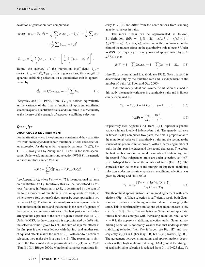
is a U-shaped function of the number of traits (Fig. 1C). The
expression for the inverse of the strength of apparent stabilizing
selection under multivariate quadratic stabilizing selection was
given by Zhang and Hill (2003)
VST = VS16VSλ
2 + 3n2VM/(n + 2)
16VSλ2 + n2VM. (17)
The theoretical approximations are in good agreement with sim-
ulations (Fig. 1). When selection is sufficiently weak, both Gaus-
sian and quadratic stabilizing selection should be roughly the
same. This is confirmed by simulations when mutation rate is low
(i.e., λ < 0.1). The difference between Gaussian and quadratic
fitness functions emerges with increasing mutation rate. When
λ = 0.1, the apparent stabilizing selection under Gaussian sta-
bilizing selection is noticeably weaker than that under quadratic
stabilizing selection (i.e., VST is larger, see Fig. 1D) and con-
sequently VG(T) is higher (Fig. 1B) but VG(F) lower (Fig. 1C).
The agreement between simulations and approximations degen-
erates with a high mutation rate (Fig. 1A–C), or if the strength
of real stabilizing selection is reduced from 0.1 to 0.025 (i.e., VS
2 3 5 4 EVOLUTION AUGUST 2012
GENETIC VARIATION IN FITNESS
0.60
0.70
0.80
0.90
1.00
1 10 100number of traits
E(F
)0.01
0.03
0.1
A
0.001
0.01
0.1
1
10
1 10 100
number of traits
VG(T
)
B
0.0001
0.001
0.01
0.1
1 10 100number of traits
VG(F
)
C
0.1
0.03
0.01
0.0
1.0
2.0
3.0
4.0
5.0
6.0
7.0
8.0
1 10 100number of traits
VS
TD
Figure 1. Comparison between Monte-Carlo simulations and diffusion approximations of (A) mean fitness under the constant optimum,
(B) genetic variance in quantitative trait, (C) genetic variance in fitness, and (D) the inverse of the strength of apparent stabilizing selection
(VST). The diffusion approximations (solid lines) for E(F), VG(T), VG(F), and VST are from equations (14)–(17). The simulation results are
obtained for a population of size N = 1000 under real stabilizing selection of both quadratic (dashed lines) and Gaussian fitness (dotted
lines) function with VS = 5VE. The mutational variance in each quantitative trait is VM = 10−3VE per generation, and there are L = 3000
loci within the genome. Mutation rates λ = 0.01, 0.03, and 0.1 per haploid genome per generation represented by circles, triangles, and
squares, respectively. The error bars stand for standard deviations.
increased from 5VE to 20VE) even λ = 0.03 (data not shown).
This indicates that these theoretical approximations hold only
under WMSS (i.e., a low λVS/VM approximation) (cf. Burger
2000).
Estimates from empirical data indicate that the mutational
variance in quantitative traits (VM) over many traits and species
is centered around 10−3VE with a range 10−5–10−2VE, where VE
is the environmental variance (Falconer and Mackay 1996; Houle
et al. 1996; Lynch and Walsh 1998; Keightley 2004; Keightley
and Halligan 2009). Estimates of the genome wide mutation rate λ
cover a wide range for multicelluar enkaryotes. For example, those
for Caenorhabditis elegans, Drosophila, and mouse are 0.036,
0.14, and 0.9 per haploid genome per generation, respectively
(Drake et al. 1998). The width of stabilizing selection on a single
EVOLUTION AUGUST 2012 2 3 5 5

XU-SHENG ZHANG
0
0.25
0.5
0.75
1
1.25
1.5
1.75
0 0.005 0.01 0.015 0.02
rate of directionally moving optimum
VG
(T)
12410
A
2
3
4
5
6
7
8
9
0 0.005 0.01 0.015 0.02
rate of directionally moving optimum
VS
T
B
0
0.004
0.008
0.012
0.016
0.02
0.024
0.028
0 0.005 0.01 0.015 0.02
rate of directionally moving optimum
VG
(F)
E
0.5
0.6
0.7
0.8
0.9
1
0 0.005 0.01 0.015 0.02
rate of directionally moving optimum
E(F
)
1 1
2 2
4 410 10
F
0
0.01
0.02
0.03
0.04
0.05
0.06
0 0.005 0.01 0.015 0.02rate of directionally moving optimum
VG
(lnF)
C
-0.6
-0.5
-0.4
-0.3
-0.2
-0.1
0
0 0.005 0.01 0.015 0.02
rate of directionally moving optimum
E(ln
F)
D
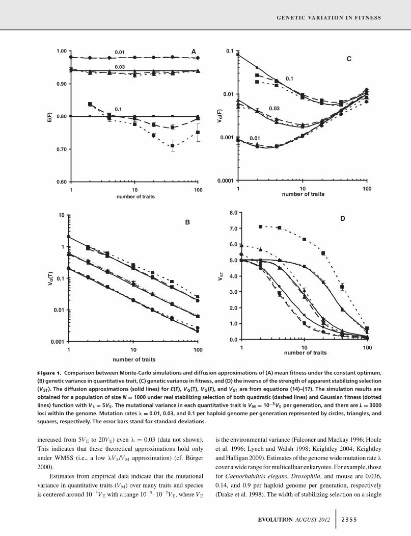
Figure 2. The influence of a directionally moving optimum on (A) genetic variance in a quantitative trait, (B) the inverse of the strength
of apparent stabilizing selection on a quantitative trait (VST), (C) genetic variance in loge fitness, (D) average of loge fitness, (E) genetic
variance in fitness, and (F) average of fitness. Results were obtained by simulations. The solid lines in panel (F) are predictions from
(20), where the values of VG(T) in panel (A) were used. Model parameters: population size N = 1000, genomic mutation rate λ = 0.03
per generation, the number of loci L = 3000, mutational variance VM = 10−3VE per generation. The n identical independent traits are
assumed to be under real stabilizing selection with a Gaussian fitness function with intrinsic strength ζ2 = 1/(2VS) = 0.1 on each trait
and moving optimum: �i(t) = kt, i = 1, . . . , n. The averages are obtained over 3000 generations at equilibrium. The error bars stand for
standard deviations. n = 1, 2, 4, and 10 traits are illustrated.
quantitative trait (VS) has been estimated as typically in the range
5–20VE (Turelli 1984; Endler 1986; Falconer and Mackay 1996;
Kingsolver et al. 2001). Assuming these typical estimates, genetic
variance in relative fitness above 0.002 can be maintained only
when λ exceeds 0.3 and the number of traits is small (i.e., n <
10) (see Fig. 1B). If λ is low and n is large but less than 1000,
however, only a very low VG(F) is maintained (Fig. 1B).
CHANGING ENVIRONMENT
To focus on the impact of a changing optimum on genetic variance,
we consider only the independent and symmetric situation where
all traits are under stabilizing selection of the same strength ζj2 =
1/(2VS), j = 1, . . . , n, have the same mutational variance VM,j =VM, and have independent and equivalent optimal values.
DIRECTIONALLY MOVING OPTIMUM
Under a directionally moving optimum, the mean phenotype in
the population responds to it with a delay (Burger 1999; Waxman
and Peck 1999),
z j,t − o j,t ≡ � = −κVS + VG(T)
VG(T), j = 1, . . . , n. (18)
Equation (18), confirmed by simulations (data not shown), can
be derived directly from the standard selection equation (Bulmer
1985 p. 151; cf. Charlesworth 1993; Burger and Lynch 1995).
Applying (18) to (8), the selective value of the mutant allele at
locus i is approximately
si ≈ Qi = −ζ2n∑
j=1
[1
2a2
i, j (1 − 2�2ζ2) − ai, j�
]. (19)
It is obvious that mutant alleles are also under directional selec-
tion: those that bring the mean phenotype closer to the optimum
will be at a selective advantage and increase in frequency. Further,
the apparent stabilizing selection on each trait is reduced (Fig. 2B;
Table S1). Therefore, VG(T) increases even though mutational ef-
fects on traits remain unchanged (Fig. 2A; Table S1; cf. Burger
1999; Waxman and Peck 1999). VG(F) also increases because
2 3 5 6 EVOLUTION AUGUST 2012

GENETIC VARIATION IN FITNESS
beneficial effects increase as the lag � increases, as suggested
by (19) (Fig. 2E; Table S1). The mean fitness reduces (Fig. 2F),
however, and when the rate κ is small, can be approximated as
E[F] =√
VS
VS + nVG(T)exp
{ −n�2
2[VS + nVG(T)]
}. (20)
Equation (20) can also be obtained directly as for (18)
(Bulmer 1985; cf. Charlesworth 1993). In terms of the impact of
a changing environment on adaptation, the results indicate that,
even though it reduces mean fitness, it facilitates the survival of
a population by increasing its variance in fitness (Gomulkiewicz
and Holt 1995).
The increases in genetic variance due to a changing relative
to a constant optimum depend on the number of traits and the
mutation rate. For example, with a rate of movement κ = 0.02σE
per generation and mutation rate λ = 0.03, the relative increase
in VG(T) is 2.6- and 5.3-fold, in VG(F) is 4.3- and 10-fold, and in
VG(lnF) is 6.6- and 26-fold for n = 1 and 10 traits, respectively. For
four traits and a rate of κ = 0.02σE, the relative increase in VG(T)
is 1.5- and 11-fold, in VG(F) 1.8- and 21-fold, and in VG(lnF) 2.5-
and 32-fold for λ = 0.1 and 0.005, respectively (cf. Waxman and
Peck 1999; Table S1). Therefore, although the genetic variances
are small for low mutation rates and many traits with a constant
optimum, directional changing optimum can boost them to large
values (Fig. 1 and Table 1).
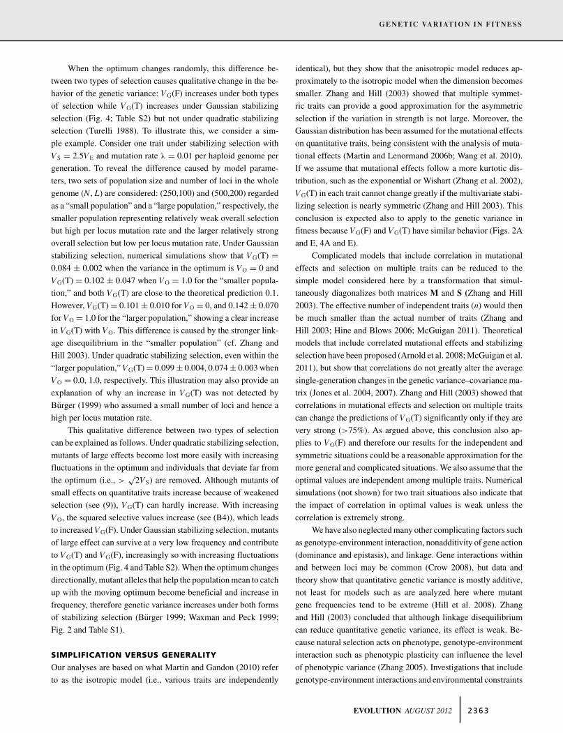
RANDOMLY VARYING OPTIMUM
The population mean phenotype responds to the optimum, but
remains behind the mean of the optimum over generations. As
an example, the standard deviation of trait mean between genera-
tions is only 0.2σE when that of the optimum over generations is√VO = 2.0σE (Fig. 3).
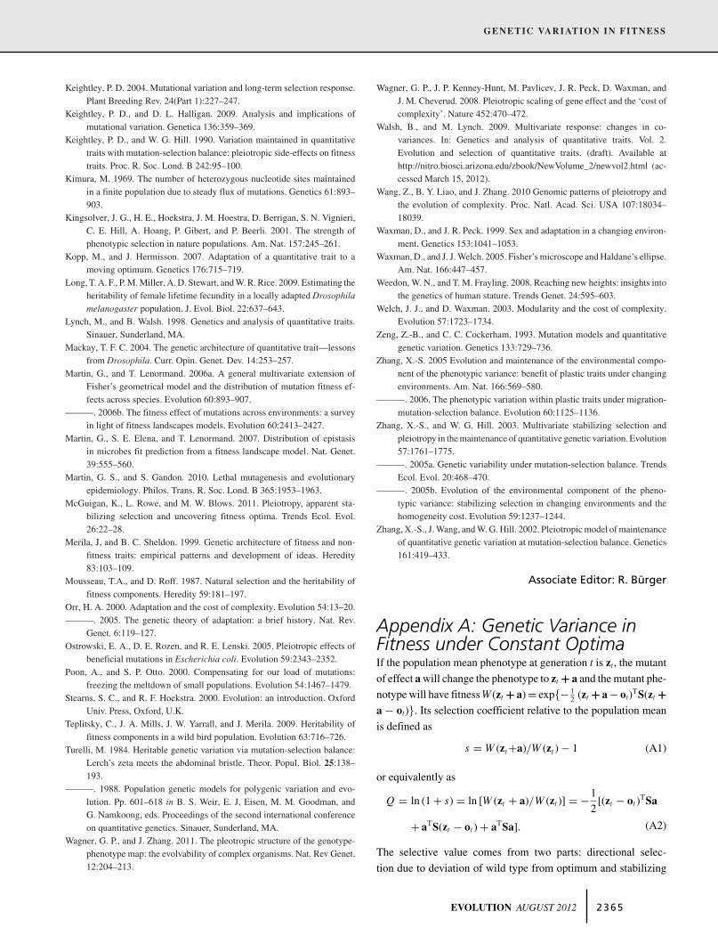
Influence of a randomly varying optimum on genetic vari-
ances in quantitative traits and fitness is shown in Figure 4. Under
Gaussian stabilizing selection, VG(T) increases with VO; when
the variance in the optimum is small (e.g., VO<<VS),
VG(T) = 4λVS
n(1 − VO/VS)(21)
(Fig. 4A; Appendix B). The underlying reason for this increase is
that the actual strength of stabilizing selection weakens (Fig. 4B).
Approximation (21) holds only under restrictive conditions be-
cause it was obtained under quadratic stabilizing selection (Ap-
pendix B). To compare it with simulation results under Gaussian
stabilizing selection the apparent stabilizing selection must be
weak so both have approximately similar effect. If overall stabi-
lizing selection is strong, Gaussian becomes much weaker than
quadratic stabilizing selection and hence (21) underpredicts sim-
ulation results for VG(T) (see Fig. 4A for n = 10). However,
if it is too weak, Kimura’s (1969) diffusion approximation for
Table 1. Comparison among four types of environmental change
on the genetic variance in quantitative traits VG(T), fitness VG(F),
and loge fitness VG(lnF). Model parameters: λ = 0.03, VS = 5VE,
N = 1000, and L = 3000. The linear regression coefficient of in-
crease in variance versus the loss of fitness is used to characterize
the increase of variance among different types of environmental
change. This estimate is obtained by using only the results from
the situations of a weakly changing optimum. The values listed
here are from analysis of Figures 2, 4–6.
Increase in variance perunit of fitness loss
Types of Number ofenvironmental change traits (n) VG(T) VG(F) VG(lnF)
Directionally moving 1 13 0.22 1.6optimum 4 2.3 0.077 0.56
10 0.87 0.031 0.14Randomly moving 1 2.4 0.17 0.34
optimum 4 0.29 0.050 0.08310 0.031 0.0049 0.012
Optimum following a 1 2.2 0.16 0.62linear stationary 4 0.76 0.027 0.29Markov process 10 0.59 0.0074 0.39
Periodically changing 1 3.2 0.17 1.2optimum 4 0.33 0.043 0.11
10 0.12 0.013 0.080
-7
-5
-3
-1
1
3
5
7
2000 2100 2200 2300
generations
op
tim
u(t
rian
gle
s), t
rait
mea
n(s
qu
ares
)
Figure 3. The change of trait mean under a randomly varying
optimum. A population of size N = 500 is started from an isogenic
state and is allowed 4N generations to reach equilibrium. The phe-
notypic mean and the optimum for trait 1 are recorded each gener-
ation. With a large standard deviation, 2.0σE, in the optimum, the
standard deviation of phenotypic mean among generations is only
about 0.2σE. Model parameters: λ = 0.05 per haploid genome per
generation, four identical independent traits under real stabilizing
selection with a Gaussian fitness function with VS = 5VE.
EVOLUTION AUGUST 2012 2 3 5 7

XU-SHENG ZHANG
0.0
0.2
0.4
0.6
0.8
1.0
1.2
0 0.5 1 1.5 2 2.5VO
VG
(T)
1 12 24 410 10
A
2
4
6
8
10
12
14
16
18
20
22
0 0.5 1 1.5 2 2.5VO
VS
T
B
0.000
0.005
0.010
0.015
0.020
0.025
0.030
0 0.5 1 1.5 2 2.5VO
V G(F
)
E
0.0
0.2
0.4
0.6
0.8
1.0
0 0.5 1 1.5 2 2.5VO
E(F
)
F
0.001
0.010
0.100
1.000
0 0.5 1 1.5 2 2.5VO
V G(ln
F)
C
-3
-2.5
-2
-1.5
-1
-0.5
0
0 0.5 1 1.5 2 2.5VO
E(ln
F)D
Figure 4. Impact of a randomly varying optimum on (A) genetic variance in a quantitative trait, (B) the inverse of the strength of
apparent stabilizing selection on a quantitative trait (VST), (C) genetic variance in loge fitness, (D) average of loge fitness, (E) genetic
variance in fitness, and (F) average of fitness. Model and simulation otherwise are as Figure 2. Results represented by dashed lines are
from simulations where the solid lines in panels (A), (E), and (F) represent theoretical approximations from equations (21), (22), and (24),
respectively. n = 1, 2, 4, and 10 traits are illustrated.
heterozygosity under strong selection (i.e., 2N|s| >> 1) breaks
down because mutations accumulate and linkage disequilibrium
and other complications reduce the genetic variance (Zhang and
Hill 2003). For one trait situation under weak overall stabilizing
selection, the prediction (21) exceeds simulation results. Further-
more, both the mutation rate and the magnitude of fluctuation in
optimum cannot be large, but for λ < 0.1 and VO < 0.4VE, (21)
agrees qualitatively with simulation results (Fig. 4A; Table S2).
The genetic variances in fitness and in loge fitness also in-
crease with VO (Fig. 4C and E). This can be understood as fol-
lows. As VO increases, the average selective value decreases (see
(9)), mutant alleles become less deleterious, and their frequencies
and heterozygosity increase. Further, VG(F) is proportional to the
mean square of fitness effects, which increase under a randomly
changing optimum (see (B4)). The two factors work together
to increase VG(F). When the variance in the optimum is small
(VO<<VS),
VG(F) = nVM
2VS(1 − VO/VS) + 8λ2
n(1 − VO/VS)2+ λVO
VS(1 − VO/VS)(22)
(Fig. 4E; Appendix B). Compared with predictions for VG(F)
in a constant environment (16), there is an extra item in (22),
λVO/(VS − VO), roughly proportional to λVO. Because VG(F)
is an integrative measure of variance in multiple traits, approx-
imation (22) holds under even more restrictive conditions than
(21) (Appendix B). Therefore, its fit to numerical simulations be-
comes less satisfactory although providing an adequate qualitative
description (Fig. 4E; Table S2).
As VO increases, the mean square difference between the
population mean and the optimum of a quantitative trait also
increases as
E((z − o)2) = 2VO
(VG(T) + VS
VG(T) + 2VS
)(23)
(Charlesworth 1993; see Fig. 4B), showing that it roughly equals
VO when VG(T) << VS. The mean fitness decreases with VO as
E[F] =√
VS
VS + nVG(T)exp
(− nVO
2[VS + nVG(T)]
)(24)
(Charlesworth 1993). The simulations agree well with this ap-
proximation (Fig. 4F).
With a randomly changing optimum, the genetic variance in
fitness can increase to substantial levels. For a constant optimum
as in Table S2 where four traits are assumed, VG(F) = 0.016
when λ = 0.1, and increases two-fold, to VG(F) = 0.031, when
2 3 5 8 EVOLUTION AUGUST 2012

GENETIC VARIATION IN FITNESS
0.0
0.2
0.4
0.6
0.8
1.0
1.2
0 0.2 0.4 0.6 0.8 1autocorrelation in optimum
V G(T
)
12410
A
1
10
100
1000
10000
100000
0 0.2 0.4 0.6 0.8 1autocorrelation in optimum
V ST
B
0
0.005
0.01
0.015
0.02
0.025
0.03
0.035
0.04
0 0.2 0.4 0.6 0.8 1autocorrelation in optimum
V G(F
)
E
0.0
0.2
0.4
0.6
0.8
1.0
0 0.2 0.4 0.6 0.8 1autocorrelation in optimum
E(F)
F
0.01
0.10
1.00
10.00
0 0.2 0.4 0.6 0.8 1
autocorrelation in optimum
V G(ln
F)
C
-18
-16
-14
-12
-10
-8
-6
-4
-2
0
0 0.2 0.4 0.6 0.8 1
autocorrelation in optimum
E(ln
F)
D
Figure 5. Influence of autocorrelation in the optimum between generations on (A) genetic variance of a quantitative trait, (B) the
inverse of the strength of apparent stabilizing selection on a quantitative trait (VST), (C) genetic variance in loge fitness, (D) average of
loge fitness, (E) genetic variance in fitness, and (F) average of fitness. Model and simulation otherwise are as Figure 2, with the optimum
following equation (4) among generations. The results were shown for the situation of n = 1, 2, 4, and 10 and for variance of white
noise δi : Vi = 1.0.
the optimum randomly changes with magnitude√
V o = 1.0σE.
As in the case of a directionally moving optimum, this relative
increase becomes substantially higher when λ becomes small,
five-fold (from VG(F) = 4.5 × 10⁻⁴ to 2.1 × 10⁻³), for example,
when λ = 0.005. The relative increase in VG(T) is compara-
tively weak. For data shown in Fig. 4, there is a 1.2- to 2.3-fold
increase in VG(T) and a 3.4- to 4.8-fold increase in VG(F) for n
increasing from 1 to 10 when the optimum randomly changes with√V o = 1.0σE. However, there is a substantial increase in VG(lnF):
under the same conditions the increase is from six- to 32-fold as
n increases from 1 to 10.
Equations (21) and (22) were obtained assuming a randomly
and slowly changing optimum so that the population stays near
MSB. If the optimum changes drastically, the expressions become
invalid, and the capacity for adaptation from both new mutations
and segregating variance might be insufficient to enable the pop-
ulation to avoid extinction (Gomulkiewicz and Holt 1995).
MARKOV PROCESS
The impact of autocorrelation in the optimum between genera-
tions under white noise with variance V = 1.0VE is weak unless
the autocorrelation coefficient d exceeds 0.8 (Fig. 5; Table S3).
Autocorrelation significantly increases VG(T) and VG(lnF), but
reduces E(F) (Fig. 5). For example, when d = 0.9, the increase in
VG(T) is <2.2-fold for n < 10 and 4.2-fold for n = 10 traits, and
in VG(lnF) is 3.8-, 6.8-, 10-, and 24-fold for n = 1, 2, 4, and 10
traits, respectively (Fig. 5). The pattern of change in VG(F) with
autocorrelation is different. When only one or two traits are under
stabilizing selection so the total selection is not strong, autocor-
relation increases VG(F), for example, about two-fold when the
autocorrelation = 0.9. With more traits so that mutant alleles are
under strong selection, VG(F) first increases and then decreases
with autocorrelation (Fig. 5; Table S3). The different behaviors
of VG(F) and VG(lnF) with autocorrelation have the following ex-
planation. When autocorrelation increases and approaches 1.0, so
the variance of changing optimum becomes very large, the fitness
becomes very small (Fig. 5D and F) and can vary within only a
small range; while loge fitness can vary much more and VG(lnF)
can remain high. As for the above two types of changing optimum,
the relative increase becomes substantially higher as the mutation
rate becomes small (Table S3). The autocorrelation weakens the
apparent stabilizing selection (i.e., increasing the value of VST)
(Fig. 5B; Table S3).
EVOLUTION AUGUST 2012 2 3 5 9

XU-SHENG ZHANG
0
0.2
0.4
0.6
0.8
1
1.2
0 0.5 1 1.5 2 2.5 3Ampitude
V G(T
)
1
2
4
10
A
1
10
100
0 0.5 1 1.5 2 2.5 3Ampitude
VS
T
B
0
0.01
0.02
0.03
0.04
0.05
0 0.5 1 1.5 2 2.5 3Ampitude
V G(F
)
E
0
0.1
0.2
0.3
0.4
0.5
0.6
0.7
0.8
0.9
1
0 0.5 1 1.5 2 2.5 3Ampitude
E(F)
F
0.001
0.01
0.1
1
10
0 0.5 1 1.5 2 2.5 3
Ampitude
V G(ln
F)
C
-8
-7
-6
-5
-4
-3
-2
-1
0
0 0.5 1 1.5 2 2.5 3
Ampitude
E(ln
F)
D
Figure 6. Influence of a periodically changing optimum on (A) genetic variance of a quantitative trait, (B) the inverse of the strength
of apparent stabilizing selection on a quantitative trait (VST), (C) genetic variance in loge fitness, (D) average of loge fitness, (E) genetic
variance in fitness, and (F) average of fitness. Model and simulation otherwise are as Figure 2. The real stabilizing selection with a
Gaussian fitness function acts independently on each of n identical traits with independent optima changing as in equation (5) with
period P = 20 generations. The situations of n = 1, 2, 4, and 10 are illustrated.
It is illuminating to compare the optimum that follows a linear
stationary Markov process with directionally and randomly mov-
ing optima. Superficially, the moving optimum described by (4) is
just a sum of Gaussian white noise and the effects of a direction-
ally moving optimum: it reduces to the latter when the variance
of white noise (V) = 0 and to a randomly moving optimum when
the autocorrelation (d) = 0. Its variance among generations VO =V/(1 − d)2 is determined by both V and d. For small V , the in-
crease in genetic variance with autocorrelation is larger than for
large V (data not shown). If V is very small the increase of genetic
variance with autocorrelation will thus become similar to that for
a directionally moving optimum; whereas if d is very small, it will
be similar to that for a randomly moving optimum. Therefore, the
optimum that follows a linear stationary Markov process is some-
where between a directionally and a randomly moving optimum
(further supported by detailed analysis, see Table 1).
PERIODICALLY CHANGING OPTIMUM
VG(T) increases with the amplitude of the change (Fig. 6; Ta-
ble S4), as for stabilizing selection on a single trait (Burger 1999).
The increase relative to that for a constant optimum is, however,
higher with more traits: for example, for a scenario of period
P = 20 generations and amplitude A = 3σE, VG(T) increases
1.8-, 2.2-, and 4.8-fold for n = 1, 4, and 10 traits, respectively
(Fig. 6A). The overall strength of apparent stabilizing selection
on each trait reduces (i.e., VST increases), increasingly so with
more traits (Fig. 5B). The mean fitness decreases and VG(lnF)
increases with increasing amplitude. Similarly, the reduction in
E(F) is greater with more traits: for example, under the same sce-
nario, by 32%, 64%, and 83% for n = 1, 4, and 10 traits, respec-
tively (Fig. 6F) and, the relative increase in VG(lnF) is higher: 31-,
192-, and 411-fold increase, respectively (Fig. 6C). The patterns of
VG(F) with amplitude are different (Fig. 6E). When there are only
one or two traits under stabilizing selection, VG(F) increases with
amplitude, and the relative increase is about eight-fold when A =3σE. When there are more traits, mutant alleles are under strong
selection and VG(F) first increases with increasing amplitude to
a maximum, then decreases. VG(lnF) and VG(F) behave differ-
ently because fitness values are extremely low if the optimum is
autocorrelated among generations. As in the above three types of
environmental change, the relative increase becomes higher when
the mutation rate becomes small (Table S4). Numerical simula-
tions show that variances change more with the amplitude than
with the period (data not shown), so we do not show the results
for changing patterns with different periods.
2 3 6 0 EVOLUTION AUGUST 2012

GENETIC VARIATION IN FITNESS
DiscussionAlthough variance in fitness is the fuel of adaptation (Fisher 1958)
and fitness is fundamental to our understanding of adaptation, our
knowledge is very limited of what determines fitness and how it
relates to other quantitative traits. To understand how the genetic
variance in fitness can be sufficient for adaptation, in this study
fitness is quantified via multivariate stabilizing selection in accor-
dance with Fisher’s geometrical model. To simplify the analysis,
we assume random mating, free recombination, additivity within
and between loci, and strengths of both stabilizing selection and
mutational effects on traits are uncorrelated, as are those between
them. Our investigations show that, in a constant environment, a
high level of genetic variance in fitness can be maintained under
MSB only in populations that have a high mutation rate. If, how-
ever, there is a changing optimum, stabilizing selection can lead
to a considerable increase in the level of genetic variance in fit-
ness, although mean fitness is reduced. This increase in variance
relative to that in a constant environment is large when the mu-
tation rate is low, and therefore MSB in a changing environment
can maintain sufficient genetic variance in fitness for adaptation.
Whereas intuitive and naıve theory based on the simple action of
natural selection predicts that variance in fitness would be lost,
in contrast to empirical observations, our more detailed investiga-
tions show this paradox vanishes and that variance is available in
the face of strong selection.
ADAPTATION VERSUS COMPLEXITY
In a constant environment, it is well known that the mean fitness
is simply determined by the mutation rate (the mutation load is
twice the mutation rate under WMSS, Haldane 1932). The mean
fitness is therefore independent of the number (n) of independent
traits under selection (i.e., “organismal complexity,” or degree
of pleiotropy [Orr 2000]), however, its genetic variance VG(F) is
closely associated with n. We found that VG(F) is determined by
two components. The first is the input of new mutations, which
is proportional to the mutational variance in quantitative traits
(VM), while the second can be understood as the contribution
from their standing genetic variance and is proportional to the
square of the genomic mutation rate (see (13), (16) and Fig. 1C).
These two components are related. For example, organisms which
have a high mutation rate may have a high VM and therefore can
maintain high VG(F) and have high capacity of adaptation to a
changing environment.
The VG(F) is influenced by organismal complexity through a
U-shaped relationship because with increasing organismal com-
plexity the first component increases but the second decreases.
The relationship stems from the so-called Euclidean superpo-
sition mutation model and MSB. In the Euclidean superposition
model, which has been supported by empirical data (Wagner et al.
2008; Wagner and Zhang 2011; Hill and Zhang 2012), mutational
effects on individual traits are independent of the total number of
traits affected and the total impact of mutations increases linearly
with the degree of pleiotropy. Thus, the total mutational variance
increases with n. (If the invariant total effect model [Orr 2000] was
assumed, this term would be constant across n values, however.)
At MSB, those mutations that affect more traits are under stronger
selection, which leads to the decrease in quantitative genetic vari-
ance (see (15)) and its consequent contribution to VG(F) (second
term of (16)). Therefore, the initial decrease in VG(F) with n is
due to the increased selection pressure whereas the increase for
large n is due to the increased overall mutational effect, implying
that very complex organisms can have high genetic variance.
Another relevant question is: how much of VG(F) maintained
within the current environment is usable for future new environ-
ments? Unlike a quantitative trait (e.g., body weight) that is only
determined by gene effects if phenotypic plasticity is ignored, the
fitness effects of genes are also determined by the effects of the
environment on the selection applied. If we assume that fitness
effects of genes do not change dramatically when the popula-
tion changes from its current to a future new environment, the
genetic variance in fitness maintained in the current equilibrium
population can provide usable fuel for adaptation to future new
environments. Therefore the U-shaped relationship of VG(F) with
n indicates that a very complex organism can also have a high rate
of adaptation in accordance with Fisher’s fundamental theorem
(1958).
This finding is in sharp contrast to that predicted in the so-
called “cost of complexity” theory (Orr 2000) in which the rate
of adaptation decreases quickly with increasing organismal com-
plexity (i.e., n). This discrepancy arises because Orr (2000) con-
siders only the contribution of “beneficial” new mutant alleles
and, because the possibility that mutation can help populations
to catch up with the new optimum decreases with the degree of
pleiotropy (n), the rate of adaptation decreases with n. In princi-
ple, adaptation relies not only on new mutations but also on the
standing genetic variance (Crow 2008; Wagner and Zhang 2011).
Our results combine both; as the contribution from all mutations
(i.e., the first component of (16)) increases with organismal com-
plexity, the rate of adaptation does not correspondingly decrease
monotonically. For organisms that have a high mutation rate, say
one mutation per genome per generation, standing quantitative
genetic variation is the main source of VG(F) when organismal
complexity is low; with increasing organismal complexity, its
contribution decreases but that from mutation increases such that
for very complex organisms, the main contribution to adaptation
is from mutations. This argument still holds for populations in a
randomly changing environment (see (22)).
EVOLUTION AUGUST 2012 2 3 6 1

XU-SHENG ZHANG
DISTRIBUTION AND PLEIOTROPY OF MUTATIONAL
EFFECTS
For the fitness landscape determined by multivariate stabilizing
selection, the distribution of fitness effects of mutations is de-
termined by the number of independent traits under stabilizing
selection (equivalently the degree of pleiotropy). With a low de-
gree of pleiotropy, the distribution is leptokurtic (i.e., L-shaped),
and approaches the normal with increasing degree of pleiotropy
(Zhang and Hill 2003). The L-shaped distributions of mutational
effects on fitness, inferred from empirical mutational accumula-
tion and sequence data (Eyre-Walker and Keightley 2007), suggest
that the degree of pleiotropy must be small if Fisher’s geometrical
model of fitness applies. Although pleiotropy is a common phe-
nomenon (Lynch and Walsh 1998; Barton and Keightley 2002;
Mackay 2004; Ostrowski et al. 2005; Weedon and Frayling 2008;
Wagner et al. 2008; Wang et al. 2010), the degree of pleiotropy
cannot be large (Zhang and Hill 2003; McGuigan et al. 2011).
This reasoning was further supported by a detailed analysis by
Martin and Lenormand (2006a), which suggests that the number
of independent traits could be very small (n < 3) for some model
species. For such organisms with low complexity, their genetic
variance in fitness can be high only if their mutation rate is high,
say λ ≥ 0.3 mutations per haploid genome per generation.
CHANGING ENVIRONMENT AS A MAGNIFIER
No living organism lives in a constant environment, so it is impor-
tant to understand how populations respond to and are sustained
in a changing environment. To explore the impact of changing en-
vironment on the genetic variances, we only consider independent
and symmetric scenarios where independence of both stabilizing
selection and mutational effects on multiple identical traits and of
the changes in optimal values among traits is assumed.
Whether the optimum changes directionally, randomly, or pe-
riodically, the mean fitness is reduced but its variance increased.
Therefore, a changing environment drives the population to ex-
perience extinction risk by decreasing its overall fitness but com-
plements it with increasing potential to avoid it via an increased
genetic variance (Gomulkiewicz and Holt 1995). This is the con-
sequence of a complicated process. For a population in a varying
environment, the mean fitness is actually the long-term average
of mean fitness (see (11)). Although the overall mean fitness re-
mains unchanged, its mean fitness changes between generations.
With a continuous moving optimum that reduces mean fitness, it
is the increase in mean fitness by natural selection that offsets the
deterioration caused by varying environmental conditions. Under
a constant environment, most mutations are deleterious. However,
if the environment is changing, some deleterious mutants could
become beneficial and increase in frequency in a new environment
and contribute more genetic variance. It is the genetic variance
maintained in previous generations that natural selection uses to
increase mean fitness. Results (Figs. 2F, 4F, 6F, eqs. 20 and 24)
show that the increase in mean fitness can only partly recover
the mean fitness and therefore the overall mean fitness is reduced
when the population jumps to new environments.
Although our results show that the increased VG(F) does not
outweigh the effect on lowering E(F) due to deterioration of the
environment (Table 1), the increased VG(F) does provide fuel
for the population to adapt to the changing environment. Among
the four types of environmental change, which increases VG(F)
most? To answer this a unified criterion is required for measur-
ing the size of change in the optimum, but comparisons are not
straightforward because the changes have a distinct nature. Be-
cause all types of changing optimum reduce fitness, the estimate
of increase in variance per unit of mean fitness loss was used
to characterize them. For the same fitness loss, the directionally
moving optimum increases variance most (Table 1). Hence, un-
der a directionally moving optimum, the population can maintain
a high rate of adaptation and most easily retain its fitness and
survive (cf. Charlesworth 1993; Burger 1999).
For most reasonable estimates of mutation and selection pa-
rameters, the increase in VG(F) can be considerable. For example,
with a moderate magnitude of changing optimum, there could be
a two- to seven-fold increase relative to that in a constant environ-
ment when the mutation rate λ ≥ 0.03 (Figs. 2E, 4E, and 6E) and
up to 10- to 30-fold if it is assumed to be very low, say λ = 0.005
(Tables S1–S4). This behavior is similar to the results given by
Waxman and Peck (1999) and Burger and Gimelfarb (2002), who
showed for a single trait that as the mutation rate increases, the
rate of increase in VG(T) due to a directionally changing optimum
reduces. Hence, a changing environment works as a magnifier: its
impact becomes strong for populations with low mutation rate so
that their VG(F) is retained at intermediate levels. Thus, both mu-
tation and changing environment facilitate maintenance of genetic
variance (cf. Crow 2008).
GAUSSIAN VERSUS QUADRATIC FITNESS FUNCTIONS
Turelli (1988) and Burger (1999) showed for a single trait that
a randomly changing optimum cannot increase quantitative ge-
netic variance, which differs from our results (Fig. 4A, B; Ta-
ble S2). The discrepancy arises because different fitness func-
tions, quadratic in Turelli (1988) and Gaussian here, and different
parameter ranges were used (Burger 1999). In a constant envi-
ronment, these fitness functions are roughly the same under weak
selection. Otherwise the quadratic fitness function represents in-
creasingly stronger selection than the Gaussian. Then a lower
VG(T) but a higher VG(F) maintained under quadratic stabiliz-
ing selection than those under Gaussian stabilizing selection, all
others being the same (Fig. 1).
2 3 6 2 EVOLUTION AUGUST 2012
GENETIC VARIATION IN FITNESS
When the optimum changes randomly, this difference be-
tween two types of selection causes qualitative change in the be-
havior of the genetic variance: VG(F) increases under both types
of selection while VG(T) increases under Gaussian stabilizing
selection (Fig. 4; Table S2) but not under quadratic stabilizing
selection (Turelli 1988). To illustrate this, we consider a sim-
ple example. Consider one trait under stabilizing selection with
VS = 2.5VE and mutation rate λ = 0.01 per haploid genome per
generation. To reveal the difference caused by model parame-
ters, two sets of population size and number of loci in the whole
genome (N, L) are considered: (250,100) and (500,200) regarded
as a “small population” and a “large population,” respectively, the
smaller population representing relatively weak overall selection
but high per locus mutation rate and the larger relatively strong
overall selection but low per locus mutation rate. Under Gaussian
stabilizing selection, numerical simulations show that VG(T) =0.084 ± 0.002 when the variance in the optimum is VO = 0 and
VG(T) = 0.102 ± 0.047 when VO = 1.0 for the “smaller popula-
tion,” and both VG(T) are close to the theoretical prediction 0.1.
However, VG(T) = 0.101 ± 0.010 for VO = 0, and 0.142 ± 0.070
for VO = 1.0 for the “larger population,” showing a clear increase
in VG(T) with VO. This difference is caused by the stronger link-
age disequilibrium in the “smaller population” (cf. Zhang and
Hill 2003). Under quadratic stabilizing selection, even within the
“larger population,” VG(T) = 0.099 ± 0.004, 0.074 ± 0.003 when
VO = 0.0, 1.0, respectively. This illustration may also provide an
explanation of why an increase in VG(T) was not detected by
Burger (1999) who assumed a small number of loci and hence a
high per locus mutation rate.
This qualitative difference between two types of selection
can be explained as follows. Under quadratic stabilizing selection,
mutants of large effects become lost more easily with increasing
fluctuations in the optimum and individuals that deviate far from
the optimum (i.e., >√
2VS) are removed. Although mutants of
small effects on quantitative traits increase because of weakened
selection (see (9)), VG(T) can hardly increase. With increasing
VO, the squared selective values increase (see (B4)), which leads
to increased VG(F). Under Gaussian stabilizing selection, mutants
of large effect can survive at a very low frequency and contribute
to VG(T) and VG(F), increasingly so with increasing fluctuations
in the optimum (Fig. 4 and Table S2). When the optimum changes
directionally, mutant alleles that help the population mean to catch
up with the moving optimum become beneficial and increase in
frequency, therefore genetic variance increases under both forms
of stabilizing selection (Burger 1999; Waxman and Peck 1999;
Fig. 2 and Table S1).
SIMPLIFICATION VERSUS GENERALITY
Our analyses are based on what Martin and Gandon (2010) refer
to as the isotropic model (i.e., various traits are independently
identical), but they show that the anisotropic model reduces ap-
proximately to the isotropic model when the dimension becomes
smaller. Zhang and Hill (2003) showed that multiple symmet-
ric traits can provide a good approximation for the asymmetric
selection if the variation in strength is not large. Moreover, the
Gaussian distribution has been assumed for the mutational effects
on quantitative traits, being consistent with the analysis of muta-
tional effects (Martin and Lenormand 2006b; Wang et al. 2010).
If we assume that mutational effects follow a more kurtotic dis-
tribution, such as the exponential or Wishart (Zhang et al. 2002),
VG(T) in each trait cannot change greatly if the multivariate stabi-
lizing selection is nearly symmetric (Zhang and Hill 2003). This
conclusion is expected also to apply to the genetic variance in
fitness because VG(F) and VG(T) have similar behavior (Figs. 2A
and E, 4A and E).
Complicated models that include correlation in mutational
effects and selection on multiple traits can be reduced to the
simple model considered here by a transformation that simul-
taneously diagonalizes both matrices M and S (Zhang and Hill
2003). The effective number of independent traits (n) would then
be much smaller than the actual number of traits (Zhang and
Hill 2003; Hine and Blows 2006; McGuigan 2011). Theoretical
models that include correlated mutational effects and stabilizing
selection have been proposed (Arnold et al. 2008; McGuigan et al.
2011), but show that correlations do not greatly alter the average
single-generation changes in the genetic variance–covariance ma-
trix (Jones et al. 2004, 2007). Zhang and Hill (2003) showed that
correlations in mutational effects and selection on multiple traits
can change the predictions of VG(T) significantly only if they are
very strong (>75%). As argued above, this conclusion also ap-
plies to VG(F) and therefore our results for the independent and
symmetric situations could be a reasonable approximation for the
more general and complicated situations. We also assume that the
optimal values are independent among multiple traits. Numerical
simulations (not shown) for two trait situations also indicate that
the impact of correlation in optimal values is weak unless the
correlation is extremely strong.
We have also neglected many other complicating factors such
as genotype-environment interaction, nonadditivity of gene action
(dominance and epistasis), and linkage. Gene interactions within
and between loci may be common (Crow 2008), but data and
theory show that quantitative genetic variance is mostly additive,
not least for models such as are analyzed here where mutant
gene frequencies tend to be extreme (Hill et al. 2008). Zhang
and Hill (2003) concluded that although linkage disequilibrium
can reduce quantitative genetic variance, its effect is weak. Be-
cause natural selection acts on phenotype, genotype-environment
interaction such as phenotypic plasticity can influence the level
of phenotypic variance (Zhang 2005). Investigations that include
genotype-environment interactions and environmental constraints
EVOLUTION AUGUST 2012 2 3 6 3

XU-SHENG ZHANG
in the model can help us understand the level of the residual vari-
ance (Teplitsky et al. 2009; McGuigan et al. 2011) and thus total
variance in fitness. Other mechanisms such as migration, het-
erogeneous environments, and heterozygote superiority certainly
contribute to genetic variance in fitness (Barton 1990; Stearns and
Hoekstra 2000; Crow 2008). Zhang (2006) showed a complex
pattern of effects of migration and heterogeneous environment:
both mutation rate and temporal variation in environment increase
quantitative genetic variance, but both migration rate and spatial
variation in environment decrease it. How these factors interact to
contribute to the variance in fitness is worth further investigation.
ConclusionAlthough many other factors (Barton 1990; Stearns and Hoekstra
2000; Crow 2008) can contribute to the maintenance of genetic
variance in fitness, our investigations show that both mutation and
changing environment are important contributors and suggest that
MSB within a changing environment is a possible mechanism for
its maintenance. Moreover, our analyses, combined with elegant
analyses of mutational effects on fitness by Martin and Lenormand
(2006a,b), lend further support to Fisher’s geometrical model as
a possible model for fitness landscape.
ACKNOWLEDGMENTSI am grateful to B. Hill for his encouragement and constructive discus-sions. I am also indebted to two anonymous reviewers, associate editorR. Burger and editor N. Barton, who made numerous comments andconstructive suggestions that greatly improved the paper.
LITERATURE CITEDArnold S. J., R. Burger, P. A. Hohenlohe, B. C. Ajie, and A. G. Jones. 2008.
Understanding the evolution and stability of the G-matrix. Evolution62:2451–2461.
Barton, N. H. 1990. Pleiotropic models of quantitative variation. Genetics124:773–782.
———. 1998. The geometry of adaptation. Nature 395:751–752.———. 2001. The role of hybridization in evolution. Mol. Ecol. 10:551–568.Barton, N. H., and P. D. Keightley. 2002. Understanding quantitative genetic
variation. Nat. Rev. Genet. 3:11–21.Bello, Y., and D. Waxman. 2006. Near-periodic substitution and the genetic
variance induced by environmental change. J. Theor. Biol. 239:152–160.Blows, M. 2007. A tale of two matrices: multivariate approaches in evolution-
ary biology. J. Evol. Biol. 20:1–8.Bulmer, M. G. 1985. The mathematical theory of quantitative genetics. 2nd
ed. Oxford Univ. PressBurger, R. 1999. Evolution of genetic variability and the advantage of sex and
recombination in changing environments. Genetics 153:1055–1069.———. 2000. The mathematical theory of selection, recombination, and mu-
tation. Wiley, Chichester, U.K.Burger, R., and A. Gimelfarb. 2002. Fluctuating environments and the role
of mutation in maintaining quantitative genetic variation. Genet. Res.80:31–46.
Burger, R., and M. Lynch. 1995. Evolution and extinction in a changingenvironment: a quantitative genetic analysis. Evolution 49:151–163.
Charlesworth, B. 1993. Directional selection and the evolution of sex andrecombination. Genet. Res. 61:205–224.
Charlesworth, B., and K. A. Hughes. 2000. The maintenance of genetic varia-tion in life history traits. Pp. 369–392 in R. S. Singh and C. B. Krimbas,eds. Evolutionary genetics: from molecules to morphology. CambridgeUniv. Press, U.K.
Crow, J. F. 2008. Maintaining evolvability. J. Genet. 87:349–353.Crow, J. F., and M. Kimura. 1963. The theory of genetic loads. Pp. 495–505
in S. J. Geerts, eds. Proceedings of the XI International Congress ofGenetics, The Hague, The Netherlands, September I963. SymposiumPublications Division, Pergamon Press, Oxford.
Drake, J. W., B. Charlesworth, D. Charlesworth, and J. F. Crow. 1998. Ratesof spontaneous mutation. Genetics 148:1667–1686.
Elena, S. F., and R. E. Lenski. 2003. Evolution experiments with microor-ganisms: the dynamics and genetic basis of adaptation. Nat. Rev. Genet.4:457–469.
Endler, J. A. 1986. Natural selection in the wild. Princeton Univ. Press,Princeton, NJ.
Eyre-Walker, A., and P. D. Keightley. 2007. The distribution of fitness effectsof new mutations. Nat. Rev. Genet 8:610–618.
Falconer, D. S., and T. F. C. Mackay. 1996. Introduction to quantitative ge-netics. 4th ed. Longman, Harlow, U.K.
Fisher, R. A. 1930. The genetical theory of natural selection. Oxford Univ.Press, Oxford, U.K.
———. 1958. The genetical theory of natural selection. Dover, New York.Fowler, K., C. Semple, N. H. Barton, and L. Partridge. 1997. Genetic variation
for total fitness in Drosophila melanogaster. Proc. R. Soc. Lond. B264:191–199.
Gilligan, D. M., and R. Frankham. 2003. Dynamics of genetic adaptation tocaptivity. Conserv. Genet. 4:189–197.
Gomulkiewicz, R., and R. Holt. 1995. When does evolution by natural selec-tion prevent extinction? Evolution 49:201–207.
Haldane, J. B. S. 1932. The causes of evolution. Longmans, London.Hereford, J., T. F. Hansen, and D. Houle. 2004. Comparing strengths of
directional selection: how strong is strong? Evolution 58:2133–2143.Hermisson, J., and G. P. Wagner. 2004. The population genetic theory of
hidden variation and genetic robustness. Genetics 168:2271–2284.Hill, W. G., and X.-S. Zhang. 2008. Maintaining variation in fitness. Pp. 59–
81 in J. van der Werf, R. Frankham, H. Graser, and C. Gondro, eds.Adaptation and fitness in animal populations, evolutionary and breedingperspectives on genetic resource management. Springer, New york, NY.
———. 2012. On the pleiotropic structure of the genotype- pheno-type map and the evolvability of complex organism. Genetics.doi:10.1534/genetics.111.135681 [Epub ahead of print].
Hill, W. G., M. E. Goddard, and P. M. Visscher. 2008. Data and theory pointto mainly additive genetic variance for complex traits. PLoS Genet.4:e1000008.
Hine, E., and M. Blows. 2006. Determining the effective dimensionality ofthe genetic variance–covariance matrix. Genetics 173:1135–1144.
Houle, D. 1992. Comparing evolvability and variability of quantitative traits.Genetics 139:195–204.
Houle, D., B. Morikawa, and M. Lynch. 1996. Comparing mutational vari-abilities. Genetics 143:1467–1483.
Johnson, T., and N. H. Barton. 2005. Theoretical models of selection andmutation on quantitative traits. Philos. Trans. R. Soc. Lond. B 360:1411–1425.
Jones A. G., S. J. Arnold, and R. Burger. 2004. Evolution and stability of theG-matrix on a landscape with a moving optimum. Evolution 58:1639–1654.
———. 2007. The mutation matrix and the evolution of evolvability. Evolu-tion 61:727–745.
2 3 6 4 EVOLUTION AUGUST 2012
GENETIC VARIATION IN FITNESS
Keightley, P. D. 2004. Mutational variation and long-term selection response.Plant Breeding Rev. 24(Part 1):227–247.
Keightley, P. D., and D. L. Halligan. 2009. Analysis and implications ofmutational variation. Genetica 136:359–369.
Keightley, P. D., and W. G. Hill. 1990. Variation maintained in quantitativetraits with mutation-selection balance: pleiotropic side-effects on fitnesstraits. Proc. R. Soc. Lond. B 242:95–100.
Kimura, M. 1969. The number of heterozygous nucleotide sites maintainedin a finite population due to steady flux of mutations. Genetics 61:893–903.
Kingsolver, J. G., H. E., Hoekstra, J. M. Hoestra, D. Berrigan, S. N. Vignieri,C. E. Hill, A. Hoang, P. Gibert, and P. Beerli. 2001. The strength ofphenotypic selection in nature populations. Am. Nat. 157:245–261.
Kopp, M., and J. Hermisson. 2007. Adaptation of a quantitative trait to amoving optimum. Genetics 176:715–719.
Long, T. A. F., P. M. Miller, A. D. Stewart, and W. R. Rice. 2009. Estimating theheritability of female lifetime fecundity in a locally adapted Drosophilamelanogaster population. J. Evol. Biol. 22:637–643.
Lynch, M., and B. Walsh. 1998. Genetics and analysis of quantitative traits.Sinauer, Sunderland, MA.
Mackay, T. F. C. 2004. The genetic architecture of quantitative trait—lessonsfrom Drosophila. Curr. Opin. Genet. Dev. 14:253–257.
Martin, G., and T. Lenormand. 2006a. A general multivariate extension ofFisher’s geometrical model and the distribution of mutation fitness ef-fects across species. Evolution 60:893–907.
———. 2006b. The fitness effect of mutations across environments: a surveyin light of fitness landscapes models. Evolution 60:2413–2427.
Martin, G., S. E. Elena, and T. Lenormand. 2007. Distribution of epistasisin microbes fit prediction from a fitness landscape model. Nat. Genet.39:555–560.
Martin, G. S., and S. Gandon. 2010. Lethal mutagenesis and evolutionaryepidemiology. Philos. Trans. R. Soc. Lond. B 365:1953–1963.
McGuigan, K., L. Rowe, and M. W. Blows. 2011. Pleiotropy, apparent sta-bilizing selection and uncovering fitness optima. Trends Ecol. Evol.26:22–28.
Merila, J, and B. C. Sheldon. 1999. Genetic architecture of fitness and non-fitness traits: empirical patterns and development of ideas. Heredity83:103–109.
Mousseau, T.A., and D. Roff. 1987. Natural selection and the heritability offitness components. Heredity 59:181–197.
Orr, H. A. 2000. Adaptation and the cost of complexity. Evolution 54:13–20.———. 2005. The genetic theory of adaptation: a brief history. Nat. Rev.
Genet. 6:119–127.Ostrowski, E. A., D. E. Rozen, and R. E. Lenski. 2005. Pleiotropic effects of
beneficial mutations in Escherichia coli. Evolution 59:2343–2352.Poon, A., and S. P. Otto. 2000. Compensating for our load of mutations:
freezing the meltdown of small populations. Evolution 54:1467–1479.Stearns, S. C., and R. F. Hoekstra. 2000. Evolution: an introduction. Oxford
Univ. Press, Oxford, U.K.Teplitsky, C., J. A. Mills, J. W. Yarrall, and J. Merila. 2009. Heritability of
fitness components in a wild bird population. Evolution 63:716–726.Turelli, M. 1984. Heritable genetic variation via mutation-selection balance:
Lerch’s zeta meets the abdominal bristle. Theor. Popul. Biol. 25:138–193.
———. 1988. Population genetic models for polygenic variation and evo-lution. Pp. 601–618 in B. S. Weir, E. J, Eisen, M. M. Goodman, andG. Namkoong, eds. Proceedings of the second international conferenceon quantitative genetics. Sinauer, Sunderland, MA.
Wagner, G. P., and J. Zhang. 2011. The pleotropic structure of the genotype-phenotype map: the evolvability of complex organisms. Nat. Rev Genet.12:204–213.
Wagner, G. P., J. P. Kenney-Hunt, M. Pavlicev, J. R. Peck, D. Waxman, andJ. M. Cheverud. 2008. Pleiotropic scaling of gene effect and the ‘cost ofcomplexity’. Nature 452:470–472.
Walsh, B., and M. Lynch. 2009. Multivariate response: changes in co-variances. In: Genetics and analysis of quantitative traits. Vol. 2.Evolution and selection of quantitative traits. (draft). Available athttp://nitro.biosci.arizona.edu/zbook/NewVolume_2/newvol2.html (ac-cessed March 15, 2012).
Wang, Z., B. Y. Liao, and J. Zhang. 2010 Genomic patterns of pleiotropy andthe evolution of complexity. Proc. Natl. Acad. Sci. USA 107:18034–18039.
Waxman, D., and J. R. Peck. 1999. Sex and adaptation in a changing environ-ment. Genetics 153:1041–1053.
Waxman, D., and J. J. Welch. 2005. Fisher’s microscope and Haldane’s ellipse.Am. Nat. 166:447–457.
Weedon, W. N., and T. M. Frayling. 2008. Reaching new heights: insights intothe genetics of human stature. Trends Genet. 24:595–603.
Welch, J. J., and D. Waxman. 2003. Modularity and the cost of complexity.Evolution 57:1723–1734.
Zeng, Z.-B., and C. C. Cockerham. 1993. Mutation models and quantitativegenetic variation. Genetics 133:729–736.
Zhang, X.-S. 2005 Evolution and maintenance of the environmental compo-nent of the phenotypic variance: benefit of plastic traits under changingenvironments. Am. Nat. 166:569–580.
———. 2006. The phenotypic variation within plastic traits under migration-mutation-selection balance. Evolution 60:1125–1136.
Zhang, X.-S., and W. G. Hill. 2003. Multivariate stabilizing selection andpleiotropy in the maintenance of quantitative genetic variation. Evolution57:1761–1775.
———. 2005a. Genetic variability under mutation-selection balance. TrendsEcol. Evol. 20:468–470.
———. 2005b. Evolution of the environmental component of the pheno-typic variance: stabilizing selection in changing environments and thehomogeneity cost. Evolution 59:1237–1244.
Zhang, X.-S., J. Wang, and W. G. Hill. 2002. Pleiotropic model of maintenanceof quantitative genetic variation at mutation-selection balance. Genetics161:419–433.
Associate Editor: R. Burger
Appendix A: Genetic Variance inFitness under Constant OptimaIf the population mean phenotype at generation t is zt, the mutant
of effect a will change the phenotype to zt + a and the mutant phe-
notype will have fitness W(zt + a) = exp{− 12 (zt + a − ot)TS(zt +
a − ot)}. Its selection coefficient relative to the population mean
is defined as
s = W (zt+a)/W (zt ) − 1 (A1)
or equivalently as
Q = ln (1 + s) = ln [W (zt + a)/W (zt )] = −1
2[(zt − ot )
TSa
+ aTS(zt − ot ) + aTSa]. (A2)
The selective value comes from two parts: directional selec-
tion due to deviation of wild type from optimum and stabilizing
EVOLUTION AUGUST 2012 2 3 6 5

XU-SHENG ZHANG
selection due to mutation. The mean phenotype will be coincident
with the optimum when the optimum remains constant, that is,
zt = ot (Burger 2000). Assume that the n traits are independent
and identical and under independent stabilizing selection such that
S = ζ2I. Under weak selection whereby Gaussian and quadratic
fitness functions are approximately equal the selective value of
the mutation is approximately
s = −1
2
n∑j=1
a2j ζ
2. (A3)
Because of complicated interactions in fitness effects between al-
leles within and across loci (Martin et al. 2007), it is not straight-
forward to obtain the expression for VG(F) in terms of fitness
effects of mutant alleles as (6) for VG(T). However, by definition,
the variance in fitness can be expressed indirectly via mutational
effects on traits as
VG(F) ≡ E(s2) − E2(s) = ζ4n∑
k=1
n∑j=1
VGkj (T), (A4)
where the variance–covariance of the product of deviations from
mean of traits k and j under the infinite independent loci model
(Zhang et al. 2002) is
VGkj (T) = E[(zk − zk)2(z j − z j )2]− E[(zk − zk)2]E[(z j − z j )
2]
=∫ ∞
−∞· · ·∫ ∞
−∞f (a)[H (s)−3K (s)]
a2i a2
j
16da+2[Gk j (T )]2
(A5)
and the genetic variance–covariance in quantitative traits is
Gk j (T) =∫ ∞
−∞· · ·∫ ∞
−∞f (a)H (s)
aka j
4da, (A6)
(Zhang and Hill 2003). Here, f (a) is the joint distribution of mu-
tational effects on n traits. Hence, VG(F) is determined by the
product of ζ4 and the sum of fourth moments VGkj (T) of muta-
tional effects on quantitative traits. If we regard ζ2 as representing
the one-fold action of stabilizing selection, ζ4 represents the two-
fold action of stabilizing selection. This suggests that variance in
fitness is a consequence of fourth moments of mutational effects
under the two-fold action of stabilizing selection.
Expressions for heterozygosity H(s) and square of heterozy-
gosity K(s) were given by Kimura (1969). By the independence
assumption of mutational effects, the distribution f (a) reduces to
� gj(aj),
Gk j (T) = δk j VG, j (T) = δk j
∫ ∞
−∞· · ·∫ ∞
−∞
n∏j=1
g j (a j )H (s)a2
j
4da.
(A7)
Here, δkj is a Kronecker delta: δkj = 1 if k = j, δkj = 0 otherwise.
In a large population such that 2N|s|>>1, the heterozygosity at
mutation-selection-drift balance can be approximated by
H = 4λ/( − s) (A8)
and
K ∼= 0 (A9)
(Kimura 1969), where λ is the haploid genomic mutation rate. The
above expressions can be simplified as follows: genetic variance
maintained on trait j,
VG, j (T) =∫ ∞
−∞· · ·∫ ∞
−∞g1(a1) . . . gn(an)
λa2j
ζ2n∑
l=1
1
2a2
l
da,
j = 1, . . . , n,(A10)
variance–covariance of the product of deviations from mean of
traits k and j,
VGkj (T) =∫ ∞
−∞· · ·∫ ∞
−∞g1(a1) . . . gn(an)
4λn∑
l=1
1
2a2
l ζ2l
a2k a2
j
16da
+ 2δk j VG, j (T)2. (A11)
Notice that
n∑k=1
n∑j=1
a2k a2
j =(
n∑k=1
a2k
)⎛⎝ n∑j=1
a2j
⎞⎠ (A12)
and after some algebra the genetic variance in fitness
simplifies to
VG(F) = 1
2λ
n∑j=1
ζ2j
∫ ∞
−∞a2
j g j (a j )da j + 2n∑
j=1
(VG, j (T)ζ2
j
)2.
(A13)
Note that the mutational variance in trait j per generation is VM, j =12λ∫∞−∞ a2
j g j (a j )da j ,
VG(F) =n∑
j=1
ζ2j [VM, j + 2(VG, j (T)ζj)
2]. (A14)
The expression for VG,j(T) is given by Zhang and Hill (2003) for
some special situations. Under the independent and symmetric
situation of the same strength of stabilizing selection ζ2j = 1/(2VS)
and the same mutational variance VM,j = VM, j = 1, . . . , n, on all
traits
VG, j (T) = VG(T) = 4λVS/n. (A15)
VG(F) = nVM
2VS+ 8λ2
n. (A16)
Monte-Carlo simulations show that the prediction (A16) is a good
approximation to the numerical results when mutation is weak and
selection is strong (i.e., more traits under selection) (Fig. 1C).
2 3 6 6 EVOLUTION AUGUST 2012

GENETIC VARIATION IN FITNESS
Appendix B: Genetic Variance inFitness under Randomly VaryingOptimaTo simplify derivations, we consider only the situation where
the n traits have identically independent stabilizing selection and
mutational effects. We assume that the optimum ot changes ran-
domly across generations. The selective value of the mutation at
generation t can be approximated as
st ≈ Qt = −ζ2n∑
j=1
[1
2a2
j − (o j,t − z j,t )2a2
j ζ2 − (o j,t − z j,t )a j
](B1)
and its square as
s2t = ζ4
n∑j=1
[1
2a2
j − (o j,t − z j,t )2a2
j ζ2 − (o j,t − z j,t )a j
]2
+ ζ4n∑
k = j
[1
2a2
k − (ok,t − zk,t )2a2
k ζ2 − (ok,t − zk,t )ak
]
×[
1
2a2
j − (o j,t − z j,t )2a2
j ζ2 − (o j,t − z j,t )a j
], (B2)
where zj,t is the average of mean phenotype of trait j at
generation t.
If the optimum is sampled from N(0, Iσ2o), the average value
of the trait mean is zero and its variance is very small relative to
σo2 (see Fig. 3). Assuming that o j,t − z j,t , j = 1, . . . , n, are inde-
pendently normal, and averaging over a long period, the following
approximations hold,
ET[(ok,t − zk,t )2m+1(o j,t − z j,t )
2n+1] ≈ 0, m = n = 0, 1, 2 . . .
ET[(o j,t − z j,t )2] ≈ Var(o j ) = VO
ET[(o j,t − z j,t )4] ≈ 3V 2
O
ET[(ok,t − zk,t )2(o j,t − z j,t )
2] ≈ Var(ok)Var(o j ) = V 2O.
Employing these following approximations
ET
⎧⎨⎩
n∑k, j
[1
2a2
k − (ok,t − zk,t )2a2
k ζ2 − (ok,t − zk,t )ai
]
×[
1
2a2
j − (o j,t − z j,t )2a2
j ζ2 − (o j,t − z j,t )a j
]⎫⎬⎭
=n∑
k, j
{1
4a2
k a2j [1 − 2VOζ2]2 + δk j
[2V 2
Oa4j ζ
4 + VOa2j
]}
the means of selective value and its square of the mutant allele
over generations are approximated as
s ≡ ET[st ] ≈ ET[Qt ] = −ζ2n∑
j=1
[1
2a2
j (1 − 2VOζ2)
](B3)
∧s2 ≡ ET
[s2
t
] ≈ ET[Q2
t
] = ζ4
⎧⎪⎨⎪⎩⎛⎝ n∑
j=1
1
2a2
j [1 − 2VOζ2]
⎞⎠
2
+n∑
j=1
[2V 2
Oa4j ζ
4 + VOa2j
]⎫⎬⎭ , (B4)
respectively.
We assume that the optimum changes slowly and over a small
scale so that the fluctuation in s remains small and the population
remains near the MSB. The average heterozygosity over genera-
tions can then be approximated by the delta method (Lynch and
Walsh 1998) as H = 4λs
∧s2
s2 . Furthermore, use of the Fisher–Wright
transition matrix confirms that, when the magnitude of fluctua-
tion in optimum is much smaller than the width of fitness profile
(i.e., VO<<VS),∧s2 ≈ s2 and H ≈ 4λ/s. As in Appendix A, the
average genetic variance in a quantitative trait and fitness over a
long period can be approximated by
VG, j (T) =∫ ∞
−∞· · ·∫ ∞
−∞
λa2j
n∑k=1
1
2a2
k ζ2(1 − 2VOζ2)
n∏k=1
gk(ak)dak .
(B5)
VG(F) =n∑
k=1
n∑j=1
ζ2kζ
2j VGkj ≈ 1
2λζ2(1 − 2VOζ2)
×n∑
j=1
∫ ∞
−∞a2
j g j (a j )da j + λζ4∫ ∞
−∞· · ·∫ ∞
−∞
×
n∑j=1
VO[a2
j + a4j VOζ4
]n∑
k=1
12 a2
k ζ2(1 − 2VOζ2)
n∏k=1
gk(ak)dak + 2n∑
j=1
V 2G, j ζ
4
= ζ2(1 − 2VOζ2)n∑
j=1
VM, j + 2λζ2VO
(1 − 2VOζ2)+ 2λV 2
Oζ6
(1 − 2VOζ2)
×∫ ∞
−∞· · ·∫ ∞
−∞
n∑j=1
a4j
n∑k=1
a2k
n∏k=1
gk(ak)dak + 2ζ4n∑
j=1
V 2G, j .
(B6)
EVOLUTION AUGUST 2012 2 3 6 7
XU-SHENG ZHANG
Because the n traits are identically independent, and further
noting that
1
2λ
∫ ∞
−∞· · ·∫ ∞
−∞
n∑j=1
a4j
n∑k=1
a2k
n∏k=1
gk(ak)dak
<1
2λ
∫ ∞
−∞· · ·∫ ∞
−∞
⎛⎝ n∑
j=1
a2j
⎞⎠ n∏
k=1
gk(ak)dak = nVM,
by approximating the variance to the order of O(VO/VS), the above
equations reduce to
VG, j (T) = 4λVS
n(1 − VO/VS). (B7)
VG(F) = nVM
2VS(1 − VO/VS) + λVO
VS(1 − VO/VS)+ 8λ2
n(1 − VO/VS)2.
(B8)
These equations were confirmed by numerical simulations (Fig. 4)
and show that VG(T) increases with the magnitude (VO) of fluc-
tuation in the optimum while VG(F) increases with VO when
mutation rate is high, otherwise it may decrease.
Supporting InformationThe following supporting information is available for this article:
Table S1. Impact of a directionally moving optimum on VG(T), VG(F), E(F), and VST.
Table S2. Impact of a randomly varying optimum on VG(T), VG(F), E(F), and VST.
Table S3. Impact of autocorrelation in optimum between generations on VG(T), VG(F), E(F), and VST.
Table S4. Impact of a periodically changing optimum on VG(T), VG(F), E(F), and VST.
Supporting Information may be found in the online version of this article.
Please note: Wiley-Blackwell is not responsible for the content or functionality of any supporting information supplied by the
authors. Any queries (other than missing material) should be directed to the corresponding author for the article.
2 3 6 8 EVOLUTION AUGUST 2012

SUPPLEMENTARY MATERIAL
Table S1 Impact of a directionally moving optimum on VG(T), VG(F), E(F) and VST.
Simulations are obtained for population size N = 1000 where there are L = 3000 loci
on each genome and there are four identical independent traits under real stabilizing
selection of Gaussian fitness function with VS = 5VE and the optimum moving with a
rate κ. For each parameter set, six replicates were generated to obtain their means; and
only the means are shown here because standard deviations are of the order of <10%
of the means. Note that the mean fitness under fixed optimum is very close to
Haldane’s formula (i.e. equation (14)). Results are shown for four different mutation
rates (λ).
Table S1
κ=0 κ=0.005 κ=0.01 κ=0.02
λ VG(T)
0.005 0.0243 0.123 0.191 0.260
0.01 0.0534 0.147 0.199 0.281
0.03 0.170 0.234 0.302 0.368
0.1 0.616 0.733 0.831 0.943
VG(F)×103
0.005 0.445 2.46 4.97 9.45
0.01 0.595 2.63 4.82 9.37
0.03 2.26 4.37 6.69 10.6
0.1 15.6 19.8 23.3 27.5
E(F)
0.005 0.989 0.926 0.885 0.825
0.01 0.978 0.926 0.896 0.837
0.03 0.934 0.902 0.876 0.838
0.1 0.792 0.759 0.733 0.702
VST
0.005 1.96 4.00 4.87 5.77
0.01 2.90 4.71 5.08 5.84
0.03 5.01 5.56 5.76 6.18
0.1 7.02 7.47 7.86 8.37

Table S2 Impact of a randomly varying optimum on VG(T), VG(F), E(F) and VST.
Model and simulation otherwise are as Table S1. The theoretical predictions for
VG(T), VG(F), and E(F) are from equation (21), (22) and (24) respectively, which are
the diffusion approximation under quadratic stabilizing selection. Results are shown
for four different mutation rates (λ).
Table S2
VO=0 VO=0.36 VO=1.0
simulations Predictions simulations Predictions simulations Predictions
λ VG(T)
0.005 0.0243 0.025 .0307 .0269 0.0400 0.0313
0.01 0.0534 0.05 .0654 .0538 0.0775 0.0625
0.03 0.170 0.15 .181 .162 0.231 0.188
0.1 0.616 0.5 .700 .538 0.820 0.625
VG(F)×103
0.005 0.445 0.450 1.32 0.817 2.05 1.65
0.01 0.596 0.600 2.54 1.38 3.78 3.13
0.03 2.26 2.20 6.81 4.79 10.8 10.6
0.1 15.6 20.4 25.6 31.4 30.7 56.6
E(F)
0.005 0.988 0.990 0.864 0.858 0.711 0.669
0.01 0.978 0.979 0.851 0.850 0.702 0.667
0.03 0.934 0.938 0.816 0.824 0.662 0.659
0.1 0.792 0.819 0.680 0.730 0.545 0.625
VST
0.005 1.97 2.78 2.49 3.38
0.01 2.90 3.33 3.91 5.12
0.03 5.01 4.54 6.10 8.46
0.1 7.02 4.95 8.82 12.0

Table S3 Impact of autocorrelation in optimum between generations on VG(T), VG(F),
E(F) and VST. Model and simulation otherwise are as Table S1. Results are shown for
four different mutation rates (λ).
Table S3
d=0 0.2 0.6 0.8 0.9 0.95
λ VG(T)
0.005 0.0400 0.0446 0.0641 0.145 0.303 0.477
0.01 0.0775 0.0843 0.117 0.198 0.366 0.552
0.03 0.231 0.233 0.272 0.372 0.514 0.654
0.1 0.820 0.832 0.917 1.08 1.30 1.58
VG(F)×103
0.005 2.05 2.28 3.36 6.22 7.30 5.23
0.01 3.78 4.15 6.01 8.31 9.17 6.37
0.03 10.8 10.8 13.0 14.5 12.4 6.91
0.1 30.7 31.1 32.9 31.8 24.8 15.4
E(F)
0.005 .711 .698 .591 .419 .238 .111
0.01 .702 .687 .589 .414 .241 .121
0.03 .662 .654 .557 .401 .243 .112
0.1 .545 .542 .470 .360 .233 .127
VST
0.005 3.38 3.81 5.79 13.2 34.8 106
0.01 5.12 5.39 7.56 14.8 34.2 100
0.03 8.46 8.53 11.1 17.9 37.6 114
0.1 12.0 12.3 15.2 22.4 42.6 92.3

Table S4 Impact of a periodically changing optimum on VG(T), VG(F), E(F) and VST.
Model and simulation otherwise are as Table S1. Results are shown for four different
mutation rates (λ).
Table S4
A=0 1 2 3
λ VG(T)
0.005 0.024 0.032 0.066 0.105
0.01 0.053 0.071 0.130 0.178
0.03 0.170 0.198 0.319 0.365
0.1 0.616 0.717 0.973 1.20
VG(F)×103
0.005 0.454 1.69 3.65 3.56
0.01 0.596 3.49 6.57 5.40
0.03 2.26 9.44 13.7 9.17
0.1 15.6 28.8 31.9 22.1
E(F)
0.005 0.989 0.817 0.513 0.356
0.01 0.978 0.803 0.501 0.360
0.03 0.934 0.766 0.473 0.339
0.1 0.792 0.645 0.339 0.267
VST
0.005 1.96 2.72 6.92 11.3
0.01 2.90 4.16 10.4 14.2
0.03 5.01 6.80 15.0 18.7
0.1 7.02 9.58 10.6 28.5