Embed Size (px)
Citation preview

FISCAL POLICY AND THE GREAT STAGFLATION | P a g e 1
Fiscal Policy and the Great Stagflation: A Reappraisal
Steven Spadijer
Australian National University
INTRODUCTION
The 1973:IV-1975:I Stagflation remains erringly reminiscent of the Great Depression, despite
the galloping rate of inflation: each day a bank or corporation declared bankruptcy and
unemployment, particularly in the construction, rose dramatically.1 Although no Depression
eventuated, the 1973-75 inflation is frequently cited as an example of the inability of
Keynesian fiscal policy (as opposed to monetary policy) to adequately deal with recession.2
This paper argues, however, that Keynes’ quintessential proposition—that budget deficits, if
carried far enough, can halt and even reverse a precipitous decline in output—was, in fact,
conclusively demonstrated during the 1974-5 downturn.3 It notes that while the efficiency of
Big Government can be questioned, its efficacy in preventing depressions cannot.
This paper proceeds as follows. Section I shows how transfer payments stabilised incomes
and therefore employment.4 Section II examines the cash-flow benefits associated with
government deficits; deficits provide cash-flows to businesses and consumers to fulfil their
1 Arthur Burns, Talk to the U.S. Bankers Association, October 1975, Released by the Board of Governors, Federal Reserve System, Washington D.C., October 1975; for a detailed overview of the 1973-75 recession see Hyman Minsky, Stabilising An Unstable Economy (New Haven: Yale University Press, 1986) 13-16. 2 See, e.g., Greg Mankiw, Macroeconomics (New York: Worth Publishing, 2006) 56-7. 3 J.M Keynes, The General Theory Employment, Interest and Money (Cambridge: Cambridge University Press, 1936) 234 (Chapter 24). 4 This claim is generally well-accepted by the mainstream (i.e. that the deficits have positive short-run, employment effects): see, e.g. Paul Samuelson, Economics (New York: McGraw-Hill, 1973) 220-33.
FISCAL POLICY AND THE GREAT STAGFLATION | P a g e 2
debt obligations.5 Section III, then, reveals how house-holds and businesses improved their
balance-sheet position courtesy of deficit spending and thus secured funds for future
investment expenditure.6 Finally, Section IV concludes that it is thanks to Big Government
that (1) disposable income, (2) corporate profits and (3) net financial assets all rose rather
than collapsed during the 1973-75 recession; economic variables needed to avoid a 1930s
style Depression and vital for a swift, sustained economic recovery of 1976.
I. INCOME AND EMPLOYMENT EFFECTS
Government spending, even in excess of taxes, is a determinant of income. Government
expenditure, of course, is a component of aggregate demand, along with consumption and
investment, while transfer payments are not. Transfer payments merely transfer income to
individuals who generally provide no input into the production process. In standard economic
theory, government can directly add to income through tax cuts, or creating employment by
either by hiring personnel for public works or for the purpose of purchasing goods and
services through various benefits (e.g. social security payments). The economic impact of
transfer payments come only if the recipient spends the funds that are transferred i.e. they
enter into the analysis only indirectly via after tax disposable personal income and its effect
on private consumer spending. Thus, the rules governing consumption spending are
expressed as a function of disposable income, various measures of wealth and the payoff
from using income to acquire financial assets (e.g. debt repayments at a going interest rate).7
The largest dollar increase in spending during the post-war era undoubtedly occurred in
transfer payments and grants-in-aid to state and local governments. In 1950, total federal 5 On the relationship between profits and investment see Michal Kalecki, Selected Essays on Capitalism and its Dynamics (1933-1977) (Cambridge: Cambridge University Press, 1971) 175-187 (Chapter 7: ‘On Profits’). 6 Warren McClam, “Financial Fragility and Instability: Role of Lender of Last Resort” in Financial Crisis: Theory, History and Policy ed., Charles Kindleberger (Cambridge: Cambridge University Press, 1982) 130-55. 7 Samuelson, “Economics”, 220-33.

FISCAL POLICY AND THE GREAT STAGFLATION | P a g e 3
government spending was $40.8 billion (14 percent of GNP). Only $10.8 billion, i.e. 25
percent of total government spending, was transfer payments to persons. In sharp contrast, in
1975 total government spending was $356.9 billion or 24 percent of GNP; transfer payments
were $146.1 billion, i.e. 41 percent of the total government spending. Likewise, grants-in-aid
to state and local government grew rapidly, from $2.3 billion in 1950 to $54.2 billion in 1975
i.e. from 5 to 15 percent of government spending.8 Put another way, in 1975, 56 percent of
the U.S. budget was merely transferring incomes (government grants plus transfer payments).
From 1950 and 1969, total government purchases of goods and services increased by a factor
of 5, the civil government function rose by 4.51, and transfer payments to individuals
increased by a factor of almost 5 over this same period. Thus, a dramatic shift from the period
of 1950-69 and again in 1973-76 occurred in government expenditure (Figure 1).
Figure 1: U.S. Exponential Increase in Government Expenditure 1964-76
(Billions $) and Composition of Federal Government Expenditure, 1954-1974
Source: Special Budget Analysis (1976-7) (Washington: Washington DC, 1976), 15.
8 Budget of the United States: Special Analysis (Fiscal Year 1976) (Washington: Washington DC, 1976) 15-6.

FISCAL POLICY AND THE GREAT STAGFLATION | P a g e 4
The shifting nature of healthcare transfers to the elderly was particularly striking.9 In 1974,
two-thirds of all transfer payments were for retirement and disability, with old-age survival
insurance funds constituting nearly 70 percent of retirement and disability payments and 45
percent of all domestic transfer payments; in 1975, 83 percent of all transfer payments were
given to people in retirement or with a disability; in 1970 this group accounted for no more
than 35.5 percent of all welfare recipients! Further disaggregated data shows 10.3 percent of
transfer payments went to Veteran benefits and health-insurance (a rise from 6.9 percent in
1970); 13.3 percent in hospital and supplementary medical insurance (up from 6.8 percent in
1970). Furthermore, as a result of legislative measures passed in 1972, the Federal provided
direct cash assistance to the handicapped starting January 1, 1974.10 These transfers did not
exist prior to 1967, but by 1975 provided $13.3 billion to beneficiaries. Unemployment
insurance remained a mere $5.3 billion in the second quarter of 1974, it rose to $19.4 billion
during the second quarter of 1975.11
Although the unemployment rate peaked at 9 percent in June 1975 and real GNP dropped by
3.2 percent,12 in no quarter did personal disposable income decline. One reason was this is
that transfer payments. Thanks to a classical Keynesian ‘pump priming’ a quick, sustained
recovery in output occurred in early 1975. This helps explain why the downturn reversed so
quickly (i.e. in less than 18 months); a quick recovery by historical standards. In fact,
9 The following statistics and facts from here taken from “U.S. Budget: Special Analysis”, 14-17. 10 “U.S. Budget: Special Analysis”, 12-20. Also, in 1972, a 20 percent increase in benefits occurred for 27.8 million Americans; average monthly payment rose from $133 to $166 (adjusting to the CPI automatically, not to lose its real value). A $5 billion piece of Social Security package was also enacted; minimum monthly benefits of individuals employed in low income positions for at least 3 decades were raised. Increases were also made to the pensions of 3.8 million widows. The food stamp program by 1975 more than doubled its 1972 level. These ‘pay without work’ programs (for the retired and elderly) explain why inflation was rising even before the oil shock occurred (hence, the Phillip’s Curve ‘shift’ occurred because of exploding government transfer payments to poor individuals with high propensity to spend these new funds [causing inflation] just as private sector investment was collapsing [i.e. the stagnation], which allows automatic stabilisers to assert themselves); in fact, the biggest monthly rise in inflation of 21% took place 3 months prior to the oil shocks: see, Robert Barsky, “Oil and the Macro-economy Since the 1970s”, 119-20. 11 “U.S. Budget: Special Analysis”, 14, 217. 12 St. Louis Fed; Minsky, “Stabilising an Unstable Economy”, 17-20.
FISCAL POLICY AND THE GREAT STAGFLATION | P a g e 5
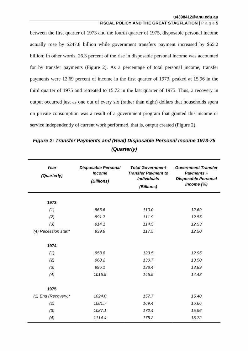
between the first quarter of 1973 and the fourth quarter of 1975, disposable personal income
actually rose by $247.8 billion while government transfers payment increased by $65.2
billion; in other words, 26.3 percent of the rise in disposable personal income was accounted
for by transfer payments (Figure 2). As a percentage of total personal income, transfer
payments were 12.69 percent of income in the first quarter of 1973, peaked at 15.96 in the
third quarter of 1975 and retreated to 15.72 in the last quarter of 1975. Thus, a recovery in
output occurred just as one out of every six (rather than eight) dollars that households spent
on private consumption was a result of a government program that granted this income or
service independently of current work performed, that is, output created (Figure 2).
Figure 2: Transfer Payments and (Real) Disposable Personal Income 1973-75
(Quarterly)
Year
(Quarterly)
Disposable Personal
Income
(Billions)
Total Government
Transfer Payment to Individuals
(Billions)
Government Transfer
Payments ÷ Disposable Personal
Income (%)
1973
(1)
(2)
(3)
(4) Recession start*
866.6
891.7
914.1
939.9
110.0
111.9
114.5
117.5
12.69
12.55
12.53
12.50
1974
(1)
(2)
(3)
(4)
953.8
968.2
996.1
1015.9
123.5
130.7
138.4
145.5
12.95
13.50
13.89
14.43
1975
(1) End (Recovery)*
(2)
(3)
(4)
1024.0
1081.7
1087.1
1114.4
157.7
169.4
172.4
175.2
15.40
15.66
15.96
15.72

FISCAL POLICY AND THE GREAT STAGFLATION | P a g e 6
Source: Economic Report of the President, January 1976, U.S. Government Printing Office,
Washington, D.C., 1976. * NBER Business Cycle Dates, Beginning and End
Furthermore, as a result the massive ‘helicopter drop’ in medical payments and grants-in-aid
funds to local and state government, we should expect sizeable increases in employment in
the healthcare, government, services, and investment in inventories independent of interest
rates decreases commencing in 1974:IV (Figure 15) i.e. before monetary policy which lags
12-18 months flows into the economy (Figure 3). This is precisely what happened. Over 800
000 new jobs in healthcare and services were created between 1973 and 1975 while over 1
100 000 were created by the government sector, the latter alone exceeding the jobs losses in
the construction sector by 350 000 people. In 1974 alone, over 600 000 government jobs
were created, that is, over quarter of the 2 000 000 new jobs that were created in healthcare in
1974, which continued to rise as the Federal deficit exploded by a further $68 billion in
1975:II:III, slightly before monetary policy was being relaxed.13
Figure 3: All Government, Services and Education and Healthcare Sector Respectively (All Employees), 1971-1977
100= Peak in Real GDP on 01/11/73; (Recession Shaded)
13 “U.S. Budget: Special Analysis”, 14-50.

FISCAL POLICY AND THE GREAT STAGFLATION | P a g e 7
Source: Reserve Bank of St. Louis (see bibliography for to access online datasets).
A robust increase in retail-trade sales and employment coincided with a sharp explosion in
cash handouts (and personal disposable income) in 1974-75 (Figure 2 and 5); indeed, retail
employment recovered even before employment in manufacturing and construction began to
recover (Figure 5). As Figure 4 also reveals, the dominant driver of real GDP growth in
1975:II-III had been the contribution of the government sector (both in public investment and
private consumption, via transfer payments). Note also the inventory investment, was
stimulated by a surge in government expenditure, as we will see in Section II.
Figure 4: GDP Growth and its Contributions to Growth, 1975:II-IV
Source: Economic Report to the President, January 1976, U.S. Government Printing
Office, Washington, D.C., 1976 40-88.
Figure 5: Retail Trade vs. Construction and Durable Manufacturing Employment 1971-77 (Peak 1/11/1973 = 100; Shaded Area is Recession)

FISCAL POLICY AND THE GREAT STAGFLATION | P a g e 8
Source: Reserve Bank of St. Louis
Thus, for the first time ever, personal disposable income rose during a severe recession
thanks to welfare programs between the private and public sectors (i.e. Keynes’ “socialisation
of investment”).14 This helps account for the dramatic rise in employment across healthcare
independent of the generally declining economic conditions during the 1973-75 period.
Transfers payments shift income to needy individuals and other end users (in healthcare,
education), which in turn use the income to finance their own purchases of goods and
services, reducing unemployment. Keynesianism was vindicated during 1973-75 recession.
Big Government prevented a Depression by giving us a stagflation: as private investment
slumped (the ‘stag’), aggressive and automatic fiscal response (far more aggressive than
today) increased personal disposable income and employment across several corporate
sectors hence, the ‘flation’)!15 We now turn to see how this stabilised output too.
14 Keynes, “The General Theory”, 245 (Chapter 24). 15 It should be noted that here I am not concerned with normative question of whether an economy where one-sixth of total disposable income is the result of state entitlements is efficient. Rather, I am concerned about the efficacy of Big Government; i.e. its employment creating “effect”. Indeed, transfer payments provide income without work but each improvement in transfer-payment schemes has the effect of raising the price at which some people will enter the labour market (however, we should also keep in mind, that the transfer payments by 1975 were made to people already retired or disabled, they accounted for 88 percent of recipients...it is unlikely that they would move into the workforce anyways; hence high unemployment cannot be blamed on transfer payments i.e. lazy, welfare bluggers). Nevertheless, the effective production capacity of the economy is eroded by decreasing labour force participation when price-deflated transfer-payments schemes are improved,

FISCAL POLICY AND THE GREAT STAGFLATION | P a g e 9
II. BUDGET DEFICITS AND CORPORATE PROFITS: CASH-FLOW EFFECTS
A basic accounting proposition is that the sum of realised financial surpluses (+) and deficits
(-) over all units must equal zero i.e. every-time some unit (e.g. the government) pays money
for the purchase of current output, some other sector (e.g. households, businesses or financial
institutions) receives that money. Therefore, if the Federal government spends $73.4 billion
more than it collects in taxes, as it did in 1975, then the sum of the deficit should re-emerge
in other sectors of the economy. This is precisely what happened in 1973-75 (Figure 6 and
7).16 The household surplus or deficit is the difference between disposable personal income
and personal outlays. Almost always, except in deep depressions (and only then in an
economy with a small government), households generate a surplus (i.e. savings rise), which
fluctuates dramatically over time. Figure 6 shows that household savings rans from 6.08
percent, 8.05, 7.52, 8.9 percent of disposable income for 1972, 73, 74 and 75 respectively.
Each jump in the household savings ratio means some other part of the economy is in deficit
i.e. being starved of potential funds. In 1973, the deficit was found in the business sector, in
1975 it was the government sector. In contrast, private business deficit is the excess of plant
and equipment, inventory, corporate housing investment over retained earnings plus capital
consumption allowances. Its deficit was $47.9 billion in 1972, jumped $79.0 billion in 1973,
remained high at $67.8 billion in 1974, and fell sharply to $21.5 billion in 1975. Business
deficits as a percentage of gross private investment, rose from 26.7 percent in 1972, 35.8
percent, 32.4 percent in 1973 and 1974 respectively, and fell 10.95 percent in 1975 (Fig. 6).
especially if, as is the case in the U.S., eligibility depends on being either unemployed or out of the labour force. Thus, although transfer payments increase disposable income, transfer payments impart an inflationary bias in the economy as demand for goods and services increases even as output and employment decreased in 1973-75; this is one reason prices kept on rising before and after the oil shocks. 16 Notwithstanding small margins of error due to data imperfections.

FISCAL POLICY AND THE GREAT STAGFLATION | P a g e 10
The path of the deficit in state, Federal and local government showed a $10 billion swing in
both 1973-74; a decrease in 1973 but an increase in 1974 and a $60 billion increase in 1975.
The $60 billion increase in 1975 must show up either as a decrease in the deficits or as an
increase in the surplus of other sectors. Part of it appeared in $15.6 billion increase in
household savings (surplus), which lead the household saving ratio being 8.92 percent of
personal disposable income. Another part showed up in huge increase of $33.1 billion in
business gross internal funds, a rise of some 23.4 percent. Indeed, in 1975, the year of a major
increase in unemployment and price-deflated GNP, gross business profits increased by 23.4
percent.17 Another component that offset the rise in the government deficit was a fall of some
$13.2 billion in investment, mainly the result of inventory liquidation. The $60 billion rise in
total government deficit easily offset the $15.6 billion rise in personal savings and a $46.3
billion decrease in the business sector deficit. In 1975 the government deficit, generated a rise
in corporate cash flows. For the first time ever in economic history, real business profits were
sustained and even increased despite the country being in a severe recession!
Figure 6: Sectoral Surpluses and Deficits, 1972-75 (Billions of Dollars)
Sectors and Their Compositions 1972 1973 1974 1975
Households
Disposable Personal Income
Personal Outlays
Personal Savings (Surplus)
Business
Gross Internal Funds
Gross Private Investment
Deficit or surplus
Government
Federal gov. deficits or surplus
State gov. deficit or surplus
Total gov. deficit or surplus
801.3
-751.9
+49.4
131.3
-179.2
-47.9
-17.3
13.7
-3.6
903.1
-830.4
+72.7
141.2
-220.2
-79.0
-6.9
12.9
+6.0
983.6
-909.5
+74.0
141.7
-209.5
-67.8
-11.7
8.1
-3.6
1076.8
-987.2
+89.6
174.8
-196.3
-21.5
-73.4
10.0
-63.4
17 Similar observations have also been made by Minsky, “Stabilising an Unstable Economy”, 30-33 and Kalecki, “Selected Essays”, 127 noting governments can bolster business profits, and thus provide available funds for future investment as savings (either by higher savings, or cutting back investment) takes place.

FISCAL POLICY AND THE GREAT STAGFLATION | P a g e 11
Total surpluses
Total deficits
Discrepancy
Household savings as % of disposable
personal income
Business deficits as % of gross private
investment
49.4
-51.5
-2.1
6.08
26.73
78.7
-79.0
-.3
8.05
35.88
74.0
-71.4
+3.6
7.52
32.4
89.6
-84.9
+4.7
8.92
10.95
Source: Economic Report to the President, January 1976, U.S. Government Printing Office,
Washington, D.C., 1976.
This rise in profits serves to emphasize how a deficit is correlated with an upward movement
toward surplus (savings) by other sectors of the economy. Gross internal funds of the
business sector ranged in the narrow band of $134.2 to $147.1 billion in the right quarters of
1973-74. No discernible trends were evident during this time. However, in the first three
quarters of 1975, as the deficit exploded, gross internal funds of business measured exploded
from $154.7, $171.8 and $185.6 billion.18 Between 1974:III and 1975:III, business gross
internal funds rose by 36.8 percent, in spite of the fall in national income and employment.
The federal government deficit was at an annual rate of $102.2 billion in the second quarter
of 1975. This deficit was $94.3 billion greater than the deficit in the second quarter of 1974,
so there had to be a $94.3 billion swing in other sectors’ surpluses or deficits in order to
offset this massive change. This swing was broken down as follows: household personal
savings rose by $40.7 billion, business gross internal funds increased by $28.2 billion and
investment fell by $30.5b. Of the total swing, some $40b was reflected in personal saving,
and some $60 billion was reflected in an increase in business internal funds or in a decrease
in business investment. Both the annual and quarterly data show that even as the economy
plunged into a deep recession the gross internal funds accruing to business actually increased!
18 Data is in annual rates, seasonally adjusted.

FISCAL POLICY AND THE GREAT STAGFLATION | P a g e 12
Thus, another reason why neoclassical economists have underappreciated the role of deficits
in the averting wide-spread economic collapse in 1974 is because private debt and profits are
generally ignored in their economic models.19 In the real world, “profits provide the internal
funds for expansion. Profits are the sinew and muscle of strength...as such they become the
immediate, unifying aim of business”20 as well as the cash-flows needed to validate business
debt.21 Because business borrowing is carried within a system of margins of safety; a
measure of such a margin is the ratio of the cash flow (profits) due on debt to the cash flow
discounted over future to the face value of outstanding debt. From 1970 to 1979, a decade of
sluggish growth but no depression, after-tax profits for 500 largest corporations increased by
300 percent, from $41 billion to $163 billion.22 In the 19th and early 20th century, an era
devoid of Big Government, a massive plunge in corporate cash-flows and hence investment
would occur. Because business and household debt-carrying capacity and the margins of
safety; lending would have decreased. Even in the absence of actual bankruptcies, such
decreases in cash flows would reduce investment commitments. Gross business profitability,
however, increased in 1975; thus a forced curtailment of commitments did not take place.23
19 See, e.g., Milton Friedman, The Optimum Quantity of Money and Other Essays (Chicago: MacMillan, 1969) 1-10; for a post-Keynesian criticism of neoclassical exclusion of debt and financial relations see, e.g., Steve Keen, “Household Debt: The Final Stage in an Artificially Extended Ponzi Scheme”, The Australian Economic Review, 42:3, 347-57; Minsky, “Stabilising an Unstable Economy”, 130-218. 20 Paul Sweezy, Monopoly Capitalism (Chicago, Monthly Review Press: 1966) 39-40. 21 Indeed, the boom of the 1970s was associated with a large increase in short-term debt issues by businesses and a proliferation of financial institutions that finance such debt issuance by issuing their own, usually short-term obligations. See, e.g., Burns, “Talk to the Economic Society”, 3-7. 22 Carol Loomis, “Profitability Goes Through a Ceiling, Fortune May 4, 1981. 23 The above examination is based on accounting identifies, which do not incorporate any behavioural relations (even though such identifies are the by-product of human behaviour). In order to understand what happened during the 1973-75 recession, we need to look at how sectoral surpluses and deficits, when summed over 0, occurred. Thus, we must formulate ideas about the determining and determined items in the accounting tables.

FISCAL POLICY AND THE GREAT STAGFLATION | P a g e 13
Sour
ce:
Eco
nom
ic R
epor
t to
the
Pre
side
nt,
Janu
ary
1976
, U
.S.
Gov
ernm
ent
Pri
ntin
g O
ffic
e, W
ashi
ngto
n, D
.C.,
1976
.
Fig
ure
7:
Sec
tora
l Su
rplu
ses
and
Def
icit
s, 1
973-
1975
(Q
uar
terl
y)
To understand why, we need to contrast consumer behaviour with business behaviour and
government budget policies. The large household savings ratios of 1974 and 1975, discussed
earlier, partly resulted in a collapse in automobiles i.e. reduction in household borrowing to
finance automobiles (which began well before the oil shock, Figure 8). If a pause takes place
in the rate at which consumer credit is extended, even as disposable income is sustained or
increased, then the saving ratio will be high as in 1975, an improvement in the liquidity
position of households will take place. With a lag, this accumulation of household liquidity
will lead to a jump in consumer spending. Those households that have not been strongly by
unemployment tend to increase the ratio to disposable income once an accumulation of liquid
assets and decrease debt relative to income. As a result of this impatience to spend, the saving

FISCAL POLICY AND THE GREAT STAGFLATION | P a g e 14
ratio is low in a recovery; the consumer—caring little about future tax increases—becomes a
“hero” leading the economy out of recession. This emblematic of a high savings ratio,
evidence that consumer behaviour is not fully passive.
Figure 8: Oil Shocks and Purchase of Automobiles
Source: Barsky and Kilian (2004), p. 122.
Nevertheless, the relation between consumer spending and present and past developments in
the economy is clear: personal outlays will almost always lie from 95 percent to 91 percent of
personal disposable income. If the savings ratio is high (8-11 percent), then it will soon be
followed by a burst of spending that lowers it toward 4-6 percent. The household saving entry
in Figure 11 and 12 is therefore largely determined by how the economy is operating and how
it has operated in the recent past; government deficits rise, however, whenever the private
sector chooses to save.24 Notice, then, how government spending in Figures 6-7 is
independent of how the economy is currently operating i.e. whereas private investment is
forward-looking, government spending operates now in the present; “coming out ahead of
workers are corporations thanks to government”.25 Hence, government spending determining
variables of growth for businesses. A fall in income due to a slump in investment or rise in 24 Congress, the state legislatures etc., pass laws that set tax laws schedules; as a result, the amount collected in taxes, given any set of tax laws, depends on behaviour of the economy. 25 Hyman Minsky, “Debt-Deflation Processes in Today’s Institutional Environment”, Vanco Nazionale de Lavoro Quarterly Review 143:4 (December 1982) 222. That is, public spending reflects government commitments independent of the business cycle and entitlement programs specifically designed to support spending during downturns, including unemployment benefits.

FISCAL POLICY AND THE GREAT STAGFLATION | P a g e 15
savings ratio will lead to automatic rise in entitlement programs and a fall in government
receipts, leading to a budget deficit. As a move toward surplus in the business sector leads to
an increase in business gross profits after tax, sustaining the debt-carrying capacity of the
business sector takes place even as the economy moves into recession. Furthermore, a large
savings ratio implies that with a lag there will be a rise in consumer spending.26
However, without Big Government, a vicious spiral between household income, household
spending, business investment, debt and cash-flows would eventuate. Private investment
would have fallen more than it did because of further inventory liquidation (which thanks to
high disposable income inventory stock was not liquidated) and a decrease, if not
abandonment, of investment programs already in progress. Disposable personal income
would have also fallen faster, even faster than personal outlays, so that the household savings
ratio would have been smaller. That is, depressions are endemic to small Government
capitalism or governments bound by harsh, austerity measures: declines in inventory
investment etc., mean both consumption and investment expenditures decrease in an effort to
eliminate debts and result in excess savings (surplus) over investment (deficits). Thus, as
construction and manufacturing workers become unemployed they cannot purchase goods
and services, employed workers (due to bad news) also save or repay their own mortgage
repayments (spurring deflation). Businesses etc., cannot meet their own debt obligations
because there are less people to purchase their goods and services; they hopelessly slash their
business margins in a feeble attempt to attract customers. As debtors repay their debts, rather
than consuming or investing, the more they owe: the decrease in the flow of business internal
26 It is interesting to note that the current savings rate is a mere 5% i.e. well below historical standards.

FISCAL POLICY AND THE GREAT STAGFLATION | P a g e 16
funds, both financial and non-financial businesses, tends to decrease investment
commitments as business slash prices, thus increasing their real debt burden.27
Figure 9: Private Investment and the Federal Deficit, 1929-30, 1933, 1974-75
1929 1930 1933 1974 1975
Gross Private Investment
Government Deficit
Total
16.2
-.9
15.3
10.1
-.9
9.2
1.4
+1.3
2.7
229
+11
240
206
+69
275
Source: Economic Report to the President, January 1985, U.S. Government Printing Office,
Washington, 1985, Table B15 and B74.
To be precise, private investment fell significantly more than one-third between 1929 and
1930; the largest decline from 1970s was only 10 percent. In both 1929 and 1930 the Federal
Government ran a surplus of some $0.90 billion. Thus, in 1930 the sum of private investment
and government deficit fell by some $6.1 billion, or 40 percent of the $15.3 billion total of
1929. In 1974 and 1975, the deficit was $11 billion and $69 billion respectively; this $58
billion increase in the deficit more than offset the $23 billion fall in private investment
(Figures 9-10). The difference between the downturns is corporate profits; in 1929, 1930,
1933 they were 10.1, 6.6 billion and -1.7 billion respectively. In 1974, corporate profits were
$83.6 billion, but in 1975 they rose to $95.9 billion!28 In 1930s the impact of government was
not able to sustain profits and therefore investment, but 1970s it sustained profits!
27 For more on the dynamics of debt-deflation see, e.g., Keen, “Artificial Ponzi Scheme”, 347-57; Irving Fischer, “The Debt Deflation Theory of Great Depressions”, Econometrica (Oct. 1933) 337-357; Irving Fischer, Booms and Depressions (New York: Adelphi, 1932). 28 Minsky, Can ‘IT’ Happen Again? (Armonk, N.Y.: M.E. Sharpe Inc., 1982), 37.

FISCAL POLICY AND THE GREAT STAGFLATION | P a g e 17
Figure 10: Private Investment and the Federal Deficit, 1929-30, 1933, 1974-75
% of GNP Year GNP Gross Private
Investment
Federal Gov.
Outlays Private Federal Gov.
1929
1933
1940
1950
1955
1960
1965
1970
1975
103.4
55.8
100.0
286.2
400.0
506.5
691.1
992.7
1549.2
16.2
1.4
13.1
53.8
68.4
75.9
113.5
144.2
206.1
2.6
4.0
10.0
40.8
68.1
93.1
123.8
204.2
356.6
15.7
2.5
13.1
18.8
17.1
15.0
16.4
14.5
13.3
2.5
7.2
10.0
14.3
17.0
18.4
17.9
20.6
23.0
Source: Same as Figure 10 (Federal Outlays and Gross PI shown in billion of $)
Thus, Big Government, with its potential for massive automatic deficits, puts a high floor on
how fast and much output can fall, particularly in a world with business and household debt
whereby corporate profits and household savings are essential to validate such debt.29 Thanks
to inflationary transfer payments (which erodes debt and fuels consumption)30 and sustain
corporate profits, the debt-carrying capacity of business and households was not severely
compromised, despite a debt to GDP ratio of 50 percent of GDP (only slightly less than in
1929).31 If it were compromised, a downward spiral of incomes and profits would led to the
debt-deflations of the past; Big Government, by providing liquidity to the business sector (via
consumers purchasing their products) validates their investments (debts), avoiding a debt-
deflation spiral. This is precisely what makes such cumulative interactive slide into a
29 See, e.g., Hyman Minsky, Can ‘IT’ Happen Again? (Armonk, N.Y.: M.E. Sharpe Inc., 1982), 30-70 (Ch. 2-3). 30 This has also been recognised in the literature as playing a role in reviving the economy. See, e.g., Mishkin, “What Depressed the Consumer?”, 166 “The one piece of good news for households was that inflation lightened their real debt burden, and that, according to Mishkin, bolstered their sagging expenditures”. The latter fails to include gov. debt is an asset! 31 Minsky, “Can IT Happen Again?”, 55.

FISCAL POLICY AND THE GREAT STAGFLATION | P a g e 18
depression a thing of the past. Thus, while the efficacy of government can be questioned; the
efficacy of inflation in preventing a depression cannot.
III. DEFICITS AND FINANCING POWER: BALANCE-SHEET EFFECTS
Government debt is a safe asset: in a fiat currency system a government cannot default on its
own public debt if it issues the debt in its own currency, irrespective of whether the bonds are
sold domestically or to foreigners (unless it chose to do so for political reasons: Japan in 1945
refused to pay out war bonds to its enemies; this is the only case ever of a default in a fiat
currency system).32 Note it was a political choice, a product not of economic necessity. This
is because, unlike during the gold standard or borrowing in a foreign currency, in a fiat
currency system a government controls the production of its own currency, so whenever a
government contract says that it will be forthcoming it will, in fact, be forthcoming.
Furthermore, government debt is marketable; its terms are guaranteed by the FED, a
guarantee that does not apply to private debt (with debtors being the user rather than
monopoly issuer of a nation’s currency). This is why post-Bretton Woods (i.e. post-1971),
fiscally sovereign nations like Japan (who control their currency production) cannot be
insolvent, nor needed tax hikes to run chronic budget deficits;33 it is why nations like Greece
or Ireland, who are not fiscally sovereign, are condemned to higher taxes unless they default.
Financial instruments are created when the government runs deficits. Thus, government debt
is a valuable source of future finance, rather than being a liability because consumers or
investors anticipate future tax increases and thereby cut back investment or increase
32 In 1946, the Chair of the New York Fed, Beardsley Ruml, also realised this point that fiat currencies do not face solvency constraints and that taxpayers do NOT fund government; government funds taxpayers (before Breton Woods the U.S. operated under a fiat system as it does today): see “Taxes For Revenue are Obsolete” <http://home.hiwaay.net/~becraft/RUMLTAXES.html> (January 1946) accessed 5 April 2010. 33 Keynes also accepted this Chartalist insight – see J.M Keynes, Treatise On Money, (New York: MacMillan, 1971) 1-10 –and partly explains why he opposed the U.K. return to the Gold Standard.

FISCAL POLICY AND THE GREAT STAGFLATION | P a g e 19
savings.34 During the 1973-75 Stagflation households and financial institutions, by acquiring
Treasury bonds etc, actually increased their net worth (Figure 11). In 1972-75 private debt
acquisition of government debt was modest; 1973 households acquired $20.4 billion in
government debt, $14.5 billion in 1974; NFI acquired a mere $3.5 billion.
Figure 11: Total Private Domestic Acquisition of U.S. Gov. Securities, 1972-75
Sector 1972 1973 1974 1975 Households
Non Financial Corporations State & Local Governments
.6 -2.4 -3.4
20.4 -1.8 -.2
14.5 3.5 -.1
-.9 16.1 -5.8
Total NFS 1.6 18.8 18.1 21.1
Commercial Banking Savings and Loans
Mutual Saving Banks Credit Unions Life Insurance
Private Pension Funds State and Local Gov. Ret.
Funds Other Investment Co.
6.5 4.3 1.4 .8 .3
1.0 -.6 -.4
-1.3 *
-.5 .2 .1 .6 .1 -.1
1.0 3.3 .1 .2 *
1.1 .6 -.3
30.3 11.1 3.6 1.9 1.3 5.4 1.7 -1.0
Total Financial Sector Total
13.6 15.2
-.4 18.4
6.7 24.9
57.1 78.1
Source: Flow of Funds Data, Board of Governors of the Fed; St Louis Reserve.
Comment/Notes: This table shows the total acquisition of government debt, Treasury
agencies combined with private domestic sectors from 1973-75 in billions of dollars. The
acquisition of gov. debt from the Fed, gov. agencies, and foreigners has been subtracted from
the total issued to derive private domestic acquisition.
In 1975, however, non-financial institutions acquired $20 billion; households decreased their
only to be dramatically outweighed by corporations who increased their holdings by $16.1
billion. In addition to government sector, financial sectors obtained, quite strikingly, some
34 Barro’s (1974) Ricardian Equivalence, a claim he repeats during every recession, says that as government spends and borrows (by issuing bonds), consumers will anticipate higher future taxes to repay such government debt and spend less now, offsetting the short-run government stimulus; thus increase saving now negates any stimulus effect coming from the budget deficits. It has time and time again been falsified empirically: see, e.g., Section II above where I show how saving drops as the boom reignites, rather than rises, as it also did in 1982 and 1990; see also Mitchell (2009a); Mitchell (2009b); Feldstein (1976); Buchannan (1976).
FISCAL POLICY AND THE GREAT STAGFLATION | P a g e 20
$57.1 billion in government debt in 1975, $50.4 billion more than in 1974; of this 50.4
billion, $30.3 billion was acquired by commercial banks and $11.1 billion in savings and loan
associations. The commercial banks and financial institutions acquired valuable assets during
1973-75 recession (Figure 12), despite wide-spread financial panic (particularly, with
REITs). By acquiring a safe asset, who value is subject to rates of inflation,35 financial
institutions were able to store their financing power and shift it from a time of slack in private
demand to some future when private demand is strong; they are assets are utilised in the
subsequent boom.
The changing composition of bank assets from 1972-75 is particularly striking. In 1973,
$52.1 billion (i.e. > 50 percent) of nets assets were banks not elsewhere classified (NEC).
Commercial banks also acquired $19.8 billion of mortgage and $10.6 billion of consumer
credit in 1973. In 1974-75 as the economy came apart, however, mortgage acquisition also
fell by 3.1 billion, while consumer credit fell by $12.9 billion. Despite this, commercial banks
acquired $32.9 billion in financial assets; $30.3 billion of it was U.S. government debt! The
banks were also able to acquire a safe asset, improve their liquidity standards, even as
aggregate income fell and bank failures took place. When government was small, a sizeable
increase in government debt held in various portfolios could not take place; a decrease in
private business debt meant a decrease in demand and time deposits. A cumulative decline in
business debt and time deposits did not occur in 1975 because there was the large and
increasing volume of public debt outstanding that could enter the portfolios of banks and
business. However, because of Big Government, via a fiat currency system, the default of
business and bank portfolios is decreased. Businesses liquidated their inventories; decreased
their indebtedness; yet banks acquired liquidity by buying government debt, rather than
35 And even during inflation periods years, bond yields were fairly constant.

FISCAL POLICY AND THE GREAT STAGFLATION | P a g e 21
decreasing assets and liabilities. The public, both households and businesses, not only
acquired safe assets in the form of bank and saving deposits, but were able to decrease their
indebtedness relative to income. The existence of large and increasing government debt acted
as a stabiliser of portfolios during the 1973-75 period, avoiding systematic financial disasters
or panic.
Figure 12: Commercial Banking: Net Acquisition of Financial Assets, 1972-75 ($ billions)
Sectors and Their Compositions 1972 1973 1974 1975
Net acqs. Of financial assets
Demand deposits + currency
Total Bank Credit
Credit-market securities
U.S. Gov securities
Direct
Agency issues
Other securities + mortgages
S&L Obligations
Corporate Bonds
Home mortgages
Other mortgages
Other cr. Excl. Security
Consumer Credit
Bank Loans
Open-market paper
Corporate Equities
Security Credit
Vault cash / member bank reserves
Other interbank claims
Miscellaneous assets
78.3
.2
75.4
70.5
6.5
2.4
4.1
25.7
7.2
1.7
9.0
7.8
38.4
10.1
28.5
-.2
.1
4.8
-1.0
1.4
2.3
100.2
.3
83.3.
86.6
-1.3
-8.8
7.6
25.9
5.7
.5
11.0
8.8
62.0
10.6
52.1
-.8
.1
-3.4
3.5
6.0
7.2
83.9
-.2
62.2
54.6
1.0
-2.6
3.6
19.1
5.5
1.1
6.5
6.1
44.5
2.8
39.5
2.2
-
-2.4
-3
7.1
15.0
32.9
*
27.8
26.6
30.3
29.1
1.2
6.4
1.3
2.1
1.9
1.2
-10.1
-.6
-12.9
3.4
-
1.2
1.0
-5.4
9.5
Source: Flow of Funds Data, Board of Governors of the Fed; St Louis Reserve.

FISCAL POLICY AND THE GREAT STAGFLATION | P a g e 22
Finally, it should be noted that the 1973-75 goes on to prove the post-Keynesian claim that,
subject to severe inflation, budget deficits dos not put upward pressure on interest rates i.e. it
does not crowd out business investment by competing with the private sector for a scarce
“finite” pool of savings (a relic left over by gold standard thinking).36 There are two reasons
for this. Firstly, budget deficits are generally a response to the endogenous workings of the
economy (i.e. the private sectors desire to save and investment which generate tax revenue),
escalating budget deficits have been associated with falling, rather than rising interest rates
(as they are now and have in Japan). Secondly, deficits add to the ‘pool’ of funds available,
generating a rise in excess reserves as a deficit explodes. Increasing net spending by
government adds to marked increase in bank reserves (Figure 14 and if nothing else happens
the overnight interest rate will be driven down by competition in the interbank market as the
commercial banks try, in vain, to eliminate the excess reserves.37 This is precisely what
happened during 1975. The operational reality, ground in the underlying national accounts, is
that the banks cannot eliminate a system-wide excess of reserves. All they can do is shuffle
the excess around between each other (Figure 14). So budget deficits put downward pressure
on interest rates across the term structure. Unsurprisingly, the discount and overnight
clearance rates were all declining as the deficit was exploding in 1975:I-IV because deficits
generate new reserves were being accurred in the banking system.
36 ‘Crowding out’ is spewed out by mainstream, neoclassical economists such as Greg Mankiw, Principles of Macroeconomics (New York: Worth Publishing, 1998) 100-12. It rests on the classical idea of a loanable funds doctrine: a fixed pool of savings. But because the money supply is an endogenous variable, that is, loans create deposits, rather than deposits creating loans (M3 leading the M1 and M0 by a full 9 months), banks are not confined to a pre-existing pool of savings, but by the credit worthiness of their borrowers. Saving is a function of income which, in turn, is a function of aggregate demand (given available aggregate supply). Bank lending is not reserve-constrained (but capital constrained) and so investment funds can be created for any credit-worthy customer at the stroke of a pen. 37 For an operational explanation of deficits are good see, Atsushi Miyanoya, “A Guide to Bank of Japan’s Market Operation”, <http://www.boj.or.jp/en/type/ronbun/ron/wps/kako/data/kwp00e03.pdf> (August 2000) accessed 3 March 2010. When there is a budget deficit, reserves will be increasing beyond the “demand for funds” by the private banks. That is, there will be excess reserves – supply is greater than demand. The result is that there will be downward pressure on the overnight rate. This is because the private banks in excess will try to place the funds on the interbank market given in Japan (or any other nation); the competition between the excess reserve banks to loan those funds out drives the overnight rate down.

FISCAL POLICY AND THE GREAT STAGFLATION | P a g e 23
Figure 13: Discount and Federal Funds Rate (1972-77)
Figure 14: Reserves of Depository Institutions (m. $; non-seasonally adjusted)
Source: Figure 13 and 14 Reserve Bank of St. Louis; line in Fig. 13 denotes end of
recession; rise in deficit.

FISCAL POLICY AND THE GREAT STAGFLATION | P a g e 24
IV. CONCLUSION
Mainstream economists have erroneously cited the 1973-75 Stagflation as a failure of Big
Government to deal with recession; nothing could be further from the truth. The 1973-75
recession vindicates the Keynesian’s policy prescription: deficits stabilise output.
Depressions are a thing of the past thanks to Big Government; stagflation the price we paid to
avoid that Depression. Thus, once we look at the interaction between the government and
non-government sectors, we see Big Government plays an important role in stabilising output
and employment. Moreover, inflation enabled businesses to repay their debts; deficits helped
co-ordinate future investment plans and allows consumers to continue consuming, thus
neutralising the deleterious effects of savings that occur in the non-government sector whilst
bailing out at debtors (rather than creditors) and providing safe sources of future finance. The
double-digit unemployment we saw during the 1820s, 1850s, 1870s, 1890s, 1930s was
successfully averted, despite the business cycle retaining trends like rental vacancies of 15
percent (that made construction sector stagnant for several years in the mid 70s).38 With
double digit vacancy rates in the U.S, disposable income falling; and the U.S. economy
turning Japanese with high debt low-inflation environment, President Obama would do well
to remember the success that was the aggressive, Keynesian response to 1974 and 1975
recession, which he appears he is trying to replicate with his new healthcare reforms.
38 Here I make a passing observation, outside that scope of this paper, that although Ireland, Spain, Iceland, Latvia, Estonia are on the verge of depression with unemployment hovering around 20 percent (Greece, by contrast, has 11 percent unemployment); none of these nations has a fiat currency system. Surprisingly, given their support of harsh austerity measures, even the IMF have concluded that bigger deficits (i.e. Big Government) means lower falls in output, while smaller deficits mean higher falls in output: http://www.imf.org/external/pubs/ft/wp/2010/wp10111.pdf Indeed, nations with a similar sized real estate boom but have retained their fiscal sovereignty are able to keep unemployment around 6-10 percent (the U.K, America). Likewise, Australian GDP growth of recent has been mostly the result of government growth; Ken Henry was right to inform PM Rudd to “go early, go hard, go households” and most of the output has been in the government sector. Of course, the success of the Australian stimulus package was that it went to the debtors (households) rather than the finance sector: Mr Obama should have asked, if I am going to bailout banks, who exactly are they going to lend to with these ‘added funds’. Both the business and household sectors are straddled with debt. Japan learnt this the hard way: it increased its monetary base by 1.7 trillion yen but deflation persisted: further evidence that the money supply is an endogenous variable, determined by the demand for credit rather than magically set by the central bank “authorities” as claimed by Milton Friedman. For more information see Richard Koo, Balance-Sheet Recession: Japan’s Struggle With Unchartered Economics and its Global Implications (New York: Wiley Books, 2003).

FISCAL POLICY AND THE GREAT STAGFLATION | P a g e 25
References
Barro, Robert J “Are Government Bonds Net Wealth?”, Journal of Political Economy 82:6,
1095-1117.
Barro, Robert J “On the Determination of the Public Debt”, Journal of Political Economy
87:5, 940-971.
Barsky, Robert R and Killian, Lutz “Oil and the Macro-economy Since the 1970s”, Journal
of Economic Perspectives 18:4 (2004) 115-134.
Buchannan, James “Barro on Ricardian Equivalence Theorem”, Journal of Political Economy
vol. 84:2, 337-342.
Budget of the United States: Special Analysis (Fiscal Year 1975)
<http://fraser.stlouisfed.org/publications/usspa/issue/4808/download/77013/1975_budgetanal
yses.pdf> (1 January 1975) accessed 5 March 2010.
Budget of the United States: Special Analysis (Fiscal Year 1976)
<http://fraser.stlouisfed.org/publications/usspa/issue/4807/download/77012/1976_budgetanal
yses.pdf > (1 January 1976) accessed 5 March 2010.
Budget of the United States: Special Analysis (Fiscal Year 1977)
<<http://fraser.stlouisfed.org/publications/usspa/issue/4807/download/77012/1977_budgetan
alyses.pdf> (1 January 1977) accessed 5 March 2010.
Budget of the United States: Special Analysis (Fiscal Year 1978)
<http://fraser.stlouisfed.org/publications/usspa/issue/4805/download/77011/1978_budgetanal
yses.pdf > (1 January 1978) accessed 5 March 2010.
Burns, Arthur Talk to the U.S. Bankers Association, October 1975, Released by the Board of
Governors, Federal Reserve System, Washington D.C., October 1975.

FISCAL POLICY AND THE GREAT STAGFLATION | P a g e 26
Economic Report of the President, January 1976, U.S. Government Printing Office,
Washington, D.C., 1976.
Economic Report of the President, January 1985, U.S. Government Printing Office,
Washington, D.C., 1985.
Feldstein, Martin. “Percieved Wealth in Bonds and Social Security: A Comment” Journal of
Political Economy 84:2 331-336.
Fischer, Irving “The Debt Deflation Theory of Great Depressions”, Econometrica (Oct. 1933)
337-357.
Fischer, Irving Booms and Depressions (New York: Adelphi, 1932).
Friedman, Milton The Optimum Quantity of Money and Other Essays (Chicago: MacMillan,
1969).
Kalecki, Michal. Selected Essays on Capitalism and its Dynamics (1933-1977) (Cambridge:
Cambridge University Press, 1971).
Keen, Steve “Household Debt: The Final Stage in an Artificially Extended Ponzi Scheme”,
The Australian Economic Review, 42:3, 347-57.
Keynes, J.M. The General Theory Employment, Interest and Money (Cambridge: Cambridge
University Press, 1936).
Keynes, .J.M. Treatise On Money, (New York: MacMillan, 1971).
Mankiw, Greg. Macroeconomics (New York: Worth Publishing, 2006).
Mankiw, Greg. Principles of Macroeconomics (New York: Worth Publishing, 1998).

FISCAL POLICY AND THE GREAT STAGFLATION | P a g e 27
McClam, Warren. “Financial Fragility and Instability: Role of Lender of Last Resort” in
Financial Crisis: Theory, History and Policy ed., Charles Kindleberger (Cambridge:
Cambridge University Press, 1982).
Minsky, Hyman. Can ‘IT’ Happen Again? (Armonk, N.Y.: M.E. Sharpe Inc., 1982).
Minsky, Hyman. “Debt-Deflation Processes in Today’s Institutional Environment”, Vanco
Nazionale de Lavoro Quarterly Review 143:4 (December 1982).
Minsky, Hyman. Stabilising An Unstable Economy (New Haven: Yale University Press,
1986).
Mishkin, Frederic “What Depressed the Consumer? The Household Balance Sheet and the
1973-75 Recession” Brookings Paper on Economic Activity vol. 197:1 (1977) 123-174.
Mitchell, Bill. “Deficits should be cut during a recession. NOT!”
<http://bilbo.economicoutlook.net/blog/?p=6399> (November 3 2009) accessed 5 March
2010.
Mitchell, Bill. “Yummy at first, then you get fat!”
<http://bilbo.economicoutlook.net/blog/?p=8216> (February 23 2010) accessed 5 March
2010.
Mitchell, Bill. “Debates in Modern Macro Theory”
<http://bilbo.economicoutlook.net/blog/?p=3921> (August 4 2009) accessed 5 March 2010.
Miyanoya, Atsushi. “A Guide to Bank of Japan’s Market Operation”,
<http://www.boj.or.jp/en/type/ronbun/ron/wps/kako/data/kwp00e03.pdf> (August 2000)
accessed 3 March 2010.
Samuelson, Paul. Economics (New York: McGraw-Hill, 1973).

FISCAL POLICY AND THE GREAT STAGFLATION | P a g e 28
St. Louis Fed: (Data from 1972-1977: <http://research.stlouisfed.org/fred2/>) accessed 15
March 2010.
Ruml, Beardsley. “Taxes For Revenue are Obselete”
<http://home.hiwaay.net/~becraft/RUMLTAXES.html> (January 1946) accessed 5 March
2010.
Sweezy, Paul. Monopoly Capitalism (Chicago, Monthly Review Press: 1966).