Fiscal Policy and Business Cycles: An Empirical Investigationfaculty.insead.edu/fatas/myc.pdf · Fiscal Policy and Business Cycles: An Empirical Investigation ... positive, do countries

Fiscal Policy and Business Cycles:

An Empirical Investigation

Antonio Fatas and Ilian MihovINSEAD and CEPR

Abstract This paper presents an empirical study of the effects of fiscal policy. We analyzethe importance of automatic stabilizers as well as the dynamic effects of discretionary fiscal

policy. We present strong evidence in favor of the hypothesis that large governments reducethe volatility of output (total or private). The result is robust to the introduction of controls

and the adjustment for possible endogeneity problems. In the second part of the paper we

review different methods of identification of discretionary fiscal policy shocks. We find strongand persistent effects of changes in fiscal policy on economic activity.

Abstract We would like to thank Stephen Cechetti, Paul de Grauwe, the Editor, an anony-

mous referee and participants at the XIII Symposium of Moneda y Credito for their helpfulcomments on the paper.

Fiscal Policy 2

1.- Introduction

There has been renewed interest in public debates in the United States, Eu-rope or Japan about the role of fiscal policy. In the United States the discussionson the Balance Budget Amendment have questioned the role of fiscal policy as atool to stabilize business cycle fluctuations. In Europe, because of the creation ofa single currency area and the disappearance of national monetary policies, therehas been a debate around whether national fiscal policies can be substitutes formonetary policy and, if not, whether a supranational fiscal federation should becreated for that purpose. In Japan, the government has repeatedly used expan-sionary fiscal policy to boost the economy and there is no consensus on whetherit had any significant effects on the economy.

This paper conducts an empirical study of the effects of fiscal policy. Wefocus our analysis on two separate issues motivated by the above public debates.First, we look at fiscal policy as an automatic stabilizer. We want to understandthe extent to which fiscal policy helps stabilizing business cycle fluctuations. Welook at data from OECD countries to assess the effects that governments haveon the volatility of output. These estimates should provide a benchmark for thediscussion of national fiscal policies in the countries members of EMU. The secondpart of the paper looks into the dynamic effects of discretionary changes in fiscalpolicy. We construct a measure of discretionary fiscal policy and describe theestimated effects in the economy.

The paper is organized as follows. Section 2 presents some basic stylized factsfor fiscal variables for a sample of 20 OECD economies. Section 3 discusses theeffects of automatic stabilizers. Section 4 studies the dynamic effects of discre-tionary policy using quarterly data from the U.S. Section 5 concludes.

2.- Some Stylized Facts

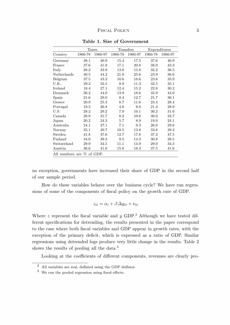
In this section we present some basic statistics on fiscal variables for a sampleof 20 OECD economies for which data on different components of fiscal policyare available.1 Table 1 shows the average size of some of the variables during oursample (1960-1997). As it is clear from the table, there are large cross countrydifferences with respect to the size and composition of the government. Also, with

1 See the appendix for data sources and definitions of variables used.

Fiscal Policy 3

Table 1. Size of Government

Taxes Transfers Expenditures

Country 1960-78 1960-97 1960-78 1960-97 1960-78 1960-97

Germany 38.1 40.9 15.4 17.5 37.6 40.9

France 37.6 41.8 17.1 20.8 38.0 43.3Italy 28.2 33.9 13.0 15.8 32.2 36.5

Netherlands 40.5 44.2 21.0 25.6 23.9 36.6

Belgium 37.5 43.3 10.6 18.6 23.8 35.9U.K. 29.2 32.5 8.9 11.3 32.5 35.1

Ireland 18.4 27.1 12.4 15.2 22.8 30.2Denmark 36.2 44.0 13.9 18.6 35.9 44.0

Spain 21.6 29.0 8.4 12.7 21.7 30.1

Greece 20.9 25.3 8.7 11.6 23.4 28.4Portugal 19.5 26.8 4.8 8.8 21.3 28.0

U.S. 28.2 29.2 7.9 10.1 30.2 31.6Canada 28.9 31.7 8.2 10.6 30.0 33.7

Japan 20.2 24.3 5.7 8.9 19.9 24.1

Australia 24.1 27.1 7.1 9.3 26.0 29.6Norway 35.1 39.7 10.5 13.8 33.8 39.3

Sweden 41.8 47.6 12.7 17.8 37.2 47.5Finland 34.0 39.3 9.5 14.3 30.8 38.5

Switzerland 29.9 34.5 11.1 14.9 29.0 34.3

Austria 36.6 41.0 15.8 18.3 37.5 41.6

All numbers are % of GDP.

no exception, governments have increased their share of GDP in the second halfof our sample period.

How do these variables behave over the business cycle? We have run regres-sions of some of the components of fiscal policy on the growth rate of GDP.

zit = αi + β∆yit + νit

Where z represent the fiscal variable and y GDP.2 Although we have tested dif-ferent specifications for detrending, the results presented in the paper correspondto the case where both fiscal variables and GDP appear in growth rates, with theexception of the primary deficit, which is expressed as a ratio of GDP. Similarregressions using detrended logs produce very little change in the results. Table 2shows the results of pooling all the data.3

Looking at the coefficients of different components, revenues are clearly pro-

2 All variables are real, deflated using the GDP delfator.3 We run the pooled regression using fixed effects.

Fiscal Policy 4

Table 2. Cyclicality of Fiscal Variables

zit = αi + β∆yit + νit

Dependent Variable β R2

Revenues 0.82 0.35(0.05)

Expenditures 0.03 0.13(0.005)

Primary Deficit/GDP (*) -0.26 0.30

(0.04)Taxes net of Transfers 1.42 0.24

(0.09)Disposable Income 0.70 0.46

(0.03)

Sample: 1960-1997. All variables in

growth rates except for (*)

Standard errors in parenthesesPooled regression, N = 20, T = 38.

cyclical while expenditures are acyclical. For example, a 1% increase in outputraises revenues by 0.8% and expenditures by only 0.03%. The primary deficit(measured as a ratio to GDP) decreases by 0.26 percentage points.

Rows 4 and 5 present evidence on the stabilization effect of taxes and trans-fers on disposable income. The variable taxes net of transfers has the largestelasticity with respect to GDP changes. A 1% increase in output raises taxesnet of transfers by approximately 1.42%. This is further corroborated by the lastrow, which shows that a 1% increase in output translates into 0.70% increase indisposable income. In other words, the behavior of taxes and transfers over thebusiness cycle help smoothing disposable income. This result is comparable tothe estimates of Bayoumi and Masson (1995) in regressions similar to the ones ofTable 2.4

We have also performed all the above regressions by countries. Qualitativelythe results are identical for all countries but there are differences in the responseof some of the fiscal variables to changes in GDP. Later in the paper we exploresome of the implications of these differences.

3.- Fiscal Policy: Automatic Stabilizers

3.1 Introduction

4 Also, Asdrubali et al. (1996), in the context of analyzing the insurance provided by the

federal budget, show how taxes and transfers smooth output fluctuations.

Fiscal Policy 5

In this section we explore the empirical effects of automatic stabilizers. Al-though there are several papers in the literature that look at the the theoreticaleffects of automatic stabilizers and the trade off between stabilization and effi-ciency, few of them present empirical evidence.5 We now review the literaturebefore we present our empirical estimates.

3.2 Literature Review

In most macroeconomics textbooks, fiscal policy is introduced when the con-cept of automatic stabilizers is presented in the Keynesian-cross model of outputdetermination. Automatic changes in government revenues in response to outputfluctuations help smoothing business cycles through the traditional demand mul-tiplier. In this model, the key to stabilization is the smoothing effect of taxes ondisposable income. In its simplest form, and assuming a proportional tax, whichmeans that average and marginal tax rates are the same, the size of total taxesis a good proxy for the degree of automatic stabilizers.

In a dynamic framework, these effects can vanish as long as the assumptionsof Ricardian equivalence are satisified. In a non-Ricardian world, however, one canthink about the benefits of automatic stabilizers taking place through the effectsthey have on the volatility of disposable income and how this helps to smoothconsumption. There are several recent empirical analysis that have shown how theU.S. fiscal budget plays an important role in this respect. Most of these papers arepart of the debate on the lessons for the future EMU of the stabilization benefitsprovided by the U.S. federal budget.6 These studies have focused their analysisin how taxes and transfers smooth disposable income ignoring the possible effectson GDP.

In a market-clearing dynamic general equilibrium model the role of automaticstabilizers is more intricate. The demand multiplier of static models based on theKeynesian cross is not present as such and the effects of automatic stabilizerstake place mainly through the impact that they have on the elasticity of laborsupply. Most of the stochastic RBC models that study the role of fiscal policydo not specifically analyze the role of automatic stabilizers but they measure the

5 For a theoretical analyis of automatic stabilizers see, for example, Christiano (1984). Gali

(1994) tests empirically the predictions of RBC models regarding the relationship between gov-

ernment size and volatility.6 See Sachs and Sala-i-Martin (1992), von Hagen (1992), Fatas (1998) or Asdrubali et al.

(1996).

Fiscal Policy 6

impact of government policies on the volatility of business cycles. In general, theresults of these models depend on the relative strength of two different effects. Alarger government reduces private wealth and, as a result, decreases the elasticityof labor supply to exogenous shocks. At the same time, a large government,through the distortions caused by higher taxes, reduces steady-state employmentwhich results in a higher elasticity of labor supply.

Gali (1994) calibrates an RBC model to measure the effect of government sizeon macroeconomic stability. For plausible parameter values, the effect on steady-state employment dominates the wealth effect and larger governments tend todestabilize the business cycle. In that sense, if one identifies automatic stabilizerswith the share of government expenditures (or revenues) in GDP, these resultsquestion the positive effects of automatic stabilizers. Although one could introduceseveral elements that could rescue the role of automatic stabilizers, the stylizedmodel of Gali (1994) is a good illustration on the difficulties of justifying theeffects of automatic stabilizers in a stochastic general equilibrium model.

3.3 Does Fiscal Policy Stabilize Output Fluctuations?

In this section we want to assess the effectiveness of automatic stabilizers.Do automatic stabilizers help smoothing business cycles? And if the answer ispositive, do countries that are exposed to more volatile business cycle make moreuse of these tools?

To answer the first question we could possibly take two approaches. We canbuild and estimate a dynamic model of the economy that includes the behaviorof automatic stabilizers and then study the counterfactual of measuring outputvolatility if automatic stabilizers did not exist.7 We do not follow this approachhere but instead we look, in a cross section of countries, for a measure of thedegree of automatic stabilizers that we correlate to variables that characterize thevolatility of the business cycle.

In our analysis we use several measures that intend to capture the strengthof automatic stabilizers starting with the simplest one: the size of governments.Although this is a very crude measure of automatic stabilizers it has severaladvantages. First, it is easy to measure and therefore can be easily used forcross-country comparisons. Second, although from a theoretical point of view whatmatters is the response of taxes and transfers to economic shocks, empirically this

7 This is the approach of Cohen and Follette (1999).

Fiscal Policy 7

response is very much linked to the size of governments.8

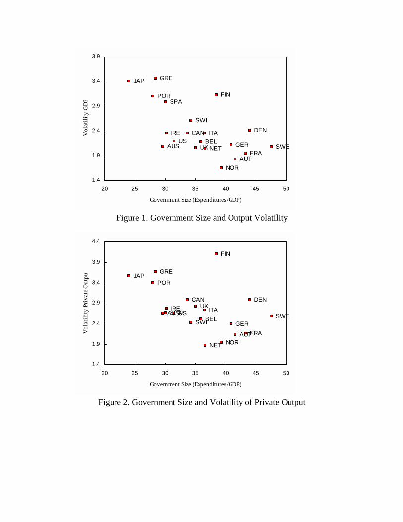
Figure 1 plots the volatility of GDP (measured as the standard deviationof real GDP growth) for 20 OECD economies against the share of governmentexpenditures in GDP. The size of the government is inversely related to thevolatility of business cycles.

[Insert Figure 1 about here]

Table 3 presents the cross section regression of the volatility of real GDPgrowth on three alternative measures of the size of the government: expenditures,taxes and transfers.9 In all cases the fit is good (with R2 over 0.4 for the caseof government expenditures) and the coefficient is significant and large. It isinteresting to see that the three measures of government size perform well and,therefore, we cannot associate the stabilization effects to a single component ofgovernment expenditures or taxes.

Table 3. Size of Government and Volatility

σ(∆y)i = α+ βGovt.Sizei + νi

Variable β R2

Expenditures -1.805 0.43(0.386)

Revenues -1.527 0.38(0.444)

Transfers -0.777 0.19

(0.283)

Sample: 1960-1997

Standard errors in parentheses

What about the correlation between government size and the volatility ofother measures of economic activity? Looking at other measures of economicactivity such as disposable income or consumption can help us understand the

8 van der Noord (2000) presents evidence for OECD countries and Fatas and Mihov (forth-

coming) for US States on the connection between government size and the cyclical elasticity of

fiscal variables.9 In all the regressions we use the logarithm of government size, measured as a ratio to GDP.

We use logarithms to argue that an increase of government size from 5 to 10 % of GDP has alarger effect on volatility than the increase between, say, 40 and 45%. Logarithmic transformation

might be seens as somewhat extreme, but in all regressions reported in the paper, we do find that

this transformation is not critical for our conclusions.

Fiscal Policy 8

mechanisms through which automatic stabilizers operate. A priori we expect theeffects of automatic stabilizers to be larger on disposable income.

Tables 4 and 5 display the results of using different measures of volatilityof economic activity.10 Surprisingly, there is no evidence that the reduction involatility is larger when we look at disposable income or consumption.

Table 4. Size of Government and Volatility of Disposable Income

σ(∆yd)i = α+ βGovt. Sizei + νi

Variable β R2

Expenditures -0.888 0.03

(0.630)Revenues -0.645 0.00

(0.703)

Transfers -0.319 0.03(0.431)

Sample: 1960-1997Standard errors in parentheses

Table 5. Size of Government and Volatility of Consumption

σ(∆c)i = α+ βGovt. Sizei + νi

Variable β R2

Expenditures -1.259 0.07

(0.848)Revenues -0.902 0.02

(0.838)

Transfers -0.649 0.03(0.624)


There is a negative correlation between the size of the government and thevolatility of disposable income but the relationship is weaker than when usingGDP. Although the size of the coefficient is practically identical to the regressionsusing GDP, both the fit of the regression and the significance of the coefficientare much lower. Same is true for consumption.

10 Volatility is again measured as the standard deviation of the growth rate.

Fiscal Policy 9

Table 6. Size of Government and Volatility of Private Output

σ(∆y)p = α+ βGovt. Sizei + νi

Variable β R2

Expenditures -1.616 0.27(0.408)

Revenues -1.339 0.22(0.474)

Transfers -0.972 0.26

(0.239)

Sample: 1960-1997

Standard errors in parentheses

What drives the negative correlation between the volatility of GDP and thesize of the government? Is is simply due to the fact that the government sectoris more stable, less subject to fluctuations? If this was the case, the explanationwould be very mechanical: a larger share on GDP simply reduces the volatilityof total output without affecting the volatility of the rest of the economy.


Figure 2 plots the volatility of private GDP (measured as GDP minus gov-ernment expenditures) against the size of the government. Surprisingly, the rela-tionship still holds and the size of the coefficient is indeed very similar. In fact,with the exception of three data points (Denmark, Finland and Sweden) all coun-tries lie very much in a straight line. This confirms that the stabilizing effects orlarger governments spread to the private sector and are not simply due to thelarger control of resources by a safe and stable government sector.

3.4 What Does Government Size Capture?

Taking as a starting point the results of the previous tables, we now introducein our analysis more direct measures of fiscal policy in order to understand theeconomic mechanisms behind the negative correlation between the size of thegovernment and the volatility of output.

We also want to know whether the size of the government is capturingautomatic stabilizers or discretionary fiscal policy. The answer to this questiondepends on what we include in the definition of automatic stabilizers. A narrowdefinition of automatic stabilizers would only include changes associated to auto-

Fiscal Policy 10

matic mechanisms built into the tax/transfer system. One of these mechanismsis the progresivity of taxes. If taxes are progressive, a 1% increase in income willincrease taxes by more than 1% and, as a result, disposable income will increaseby less than 1%.

We use marginal tax rates on labor as a direct measure of automatic stabi-lizers and check how their cross-country variation relates to the above results.11

The first thing to notice is that there is a strong correlation between average andmarginal tax rates (ρ = 0.76).

As expected, a regression of the volatility of GDP on the marginal tax rateproduces a negative and significant coefficient. If one includes in the regressionboth the average and marginal tax rate, it is difficult to conclude which one ofthe two is more relevant. In general, one finds that the coefficient for the averagetax or, more generally, the size of the government, has higher t-statistics. In mostspecifications, due to the high collinearity, both coefficients become not significant.Table 7 shows the results using government expenditures as the measure of thesize of the government.

Table 7. Marginal Tax Rate and Volatility of Output

σ(∆y)i = α+ β1 τmi + β2 Government Sizei + νi

Regression β1 β2 R2

(1) -1.127 0.20(0.458)

(2) -0.555 -2.091 0.36(0.626) (0.599)


τm: Marginal Tax Rate

We now take a broader view on automatic stabilizers and include any changein fiscal variables related to business cycles. The goal is to construct a measure ofthe responsiveness of fiscal policy to cyclical conditions and see whether this mea-sure is responsible for the correlation between size of government and volatilityof GDP.

We measure responsiveness of fiscal policy as the elasticity of fiscal variablesto GDP changes. We use the coefficients from regressing, for each country, the

11 Our measure of marginal tax rates is the marginal tax rate on labor for a single worker as

calculated in McKee et al. (1986). The value corresponds to the year 1983.

Fiscal Policy 11

growth rate of fiscal variables on the growth rate of GDP. More precisely, we runfor each country regressions similar to the one presented in Table 2.

Fiscal Indicator = α+ δ∆yt + εt (1)

Where we use as fiscal indicator the primary deficit.12 We then use the estimateδ for each country as a measure of how responsive fiscal policy is.13

The first thing to notice is that the correlation between the size of thegovernment and the responsiveness of fiscal variables (δ) is positive but moderatein size. For example, the cross-country correlation between the average ratioexpenditures to GDP and the estimates (δ) is less than 0.5.

When we regress the volatility of GDP on (δ) the significance and fit of theregression are poor. If, in addition, we include in the regression the size of thegovernment as an explanatory variable, we find that the size of the governmentalways comes always as significant and its coefficient is similar to the results ofTable 3.

Table 8. Responsiveness of Fiscal Policy and Volatility of Output

σ(∆y)i = α+ β1 δi + β2 (G/Y )i + νi

Regression β1 β2 R2

(1) -0.379 0.06(0.245)

(2) 0.141 -1.702 0.42(0.182) (0.382)


12 We have also tried the elasticity of taxes or government expenditures and obtained similar

results.13 We are aware that this regression is subject to many criticisms and possible bias. First of

all, there is a very serious issue of endogeneity. Using lagged values of output as instrumental

variables does not change the results reported below but it is unclear whether lagged values aregood instruments for such a regression. Second, and as suggested by our referee, in the presence

of trends to structural budget balances, the above regression is mispecified. We therefore theresults from this analysis should be considered as merely suggestive and we are only reporting

them because there is a large literature that has relied on estimates as the ones of equation 1

above.

Fiscal Policy 12

There are two ways of interpreting this lack of correlation between respon-siveness of fiscal policy and volatility. First, it can be that our measure of respon-siveness is a very imperfect measure of automatic stabilizers. Second, it could bethat the stabilizing properties that large governments have are unrelated to theones captured by those elasticities. One possibility, which moves us away from thenotion of automatic stabilizers, is that what the size of the government is captur-ing is the use of discretionary fiscal policy. Large governments are maybe morelikely to intervene to stabilize output.14 Of course, this assumes that discretionaryfiscal policy is succesful on stabilizing output.15

3.5 Can Other Variables Explain the Correlation

between Government Size and Volatility

Table 9. Government Size and Volatility with controls.

Dependent Variable: Volatility GDP Growth

(1) (2) (3)

Govt. Expenditures -1.805 -2.261 -1.728(3.99) (3.80) (2.11)

Openness - 0.272 -0.026(1.17) (0.08)

GDP Per Capita - -0.713

(1.38)

GDP - -0.046

(0.41)

Growth - -0.089

(0.49)

Adjusted R2 0.439 0.450 0.455

Sample: 1960-1997.t-statistics in parentheses

The results of the regressions of previous tables have shown that there is astrong negative relationship between government size and the volatility of out-

14 This is also suggested in Gali (1994).15 Notice also that, as argued above, part of this type of discretionary fiscal policy might be

already captured in the elasticity of fiscal variables to output.

Fiscal Policy 13

put. These results are suggestive, but not completely reliable. There might beadditional variables that affect both volatility and government size, and whatwe have reported so far is simply an indirect correlation between volatility andgovernment size.

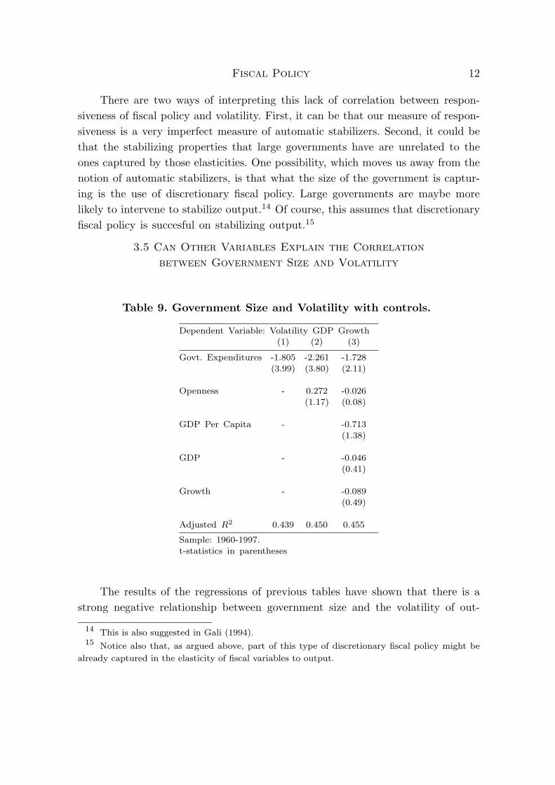
Table 9 adds several controls in the basic regression of Table 3. Column (1)presents the same coefficient as the one in Table 3.16 Column (2) of Table 9includes openness as a control. myfootnoteOpenness is measured as the averagesum of exports and imports relative to GDP for the period 1960-1997. Rodrik(1998) suggests that omitting openness from our basic regression would produce abias towards zero in the coefficient on government size. The reason is that riskiereconomies would indeed chose larger governments in order to provide enoughinsurance against the additional risk. Column (2) seems to support this view.The coefficient has increased in absolute value. One has to be careful interpretingthis regression given that the argument of Rodrik (1998) goes beyond the needto control for openness and it requires taking seriously the issue of endogeneity.We deal with this issue later in the paper by using instrumental variables.

Column (3) adds three additional controls: GDP per capita, GDP, and aver-age growth over the sample period (Growth). These three basic controls can becorrelated with both volatility and government size. First of all, richer countriestend to have larger governments because of the elasticity of government serviceswith respect to income per capita (Wagner’s Law) and an argument could bemade about the possibility that richer economies are less volatile because of moredeveloped financial systems. Size of the economy, captured by GDP, can also berelated to government size and volatility. As long as there is a fixed cost of settingup a government, smaller countries might have larger governments. The fact thatsize could also be related to volatility means that we need to control for it.17

Finally, government size and the tax distortions can affect growth, which can bea determinant of volatility. Column (3) in Table 9 shows that the introductionof these three controls does not change our basic result. Moreover, none of thecontrols are significant.

In Table 10 we report the robustness of our results to further variations of thebenchmark specification. First, we introduce two additional controls. A measure

16 In Table 9 we focus our analysis on government expenditures as a measure of government

size because it seems to be the variable with the strongest results.17 We discuss later the determinants of government size and elaborate further on these two

controls.

Fiscal Policy 14

of sectoral specialization based on Krugman (1991), which captures differencesin sectoral shares across countries.18 The second one is the standard deviation ofthe log-changes in terms of trade (ToT6097), a variable used by Rodrik (1998)as a direct measure of the additional volatility associated to openness. Althoughthere is no obvious theoretical explanation of why the absence of these controlsshould bias our basic regression, we have included them to minimize the chanceof having spurious estimate of the stabilizing role of government spending. Inboth cases, the coefficient on government size is significant and of similar size asin previous regressions.

Column (3) in Table 10 addresses the issue of possible non-linearities in theeffects of fiscal policy when governments are highly indebted. By including an in-teraction term between government size and the debt-to-GDP ratio (Debt*GY),we attempt to establish whether the stabilizing effect of government spendingdecreases as the debt-to-GDP ratio increases.19 The results are mildly support-ive of this conjecture as the coefficient is positive, although not significant atconventional levels.

Finally, columns (4) and (5) check the robustness of our result for alter-native detrending methods. In this case we calculate volatility as the standarddeviation of business cycle fluctuations as implied by GDP series detrended us-ing a Hodrick-Prescott filter. Column (5) differs from column (4) by excludingthe years 1991-1997 for Finland. The coefficient on government size is still inthe vicinity of -2 for both specifications, but the striking improvement in the fitof the regression suggests that the large economic downturn in Finland associ-ated with the collapse of the Soviet Union in the early 90’s cannot be properlytackled by the Hodrick-Prescott filter. In both cases, columns (4) and (5), thecoefficient remains significant and close in magnitude to our previous estimates.myfootnoteWe have also checked for the robustness of our results from previoustables to the detrending method. Using the Hodrick-Prescott filter does not altersignificantly any of our results.

3.6 Endogeneity of Government Size

As argued by Rodrik (1998), the size of government is endogenous to eco-nomic conditions, which casts doubts both on the unbiasedness and consistency

18 The data appendix describes the construction of this variable. It is calculated with 1991

data on sectoral production.19 We have used the average debt-to-GDP ratio for the period 1990-97.

Fiscal Policy 15

Table 10 Government Size and Volatility: Additional Controls.

Dependent Variable: Volatility GDP Growth

(1) (2) (3) (4) (5)

Govt. Expenditures -2.586 -2.344 -2.575 -1.912 -1.964

(-4.02) (-3.04) (-4.02) (-2.97) (-4.96)

Openness 0.391 0.281 0.148 0.382 0.369(1.69) (1.15) (0.58) (1.51) (2.37)

Specialization -0.328 - - - -(-1.33)

ToT6097 - -0.027 - - -

(-0.18)

Debt*GY - - 0.112 - -

(1.45)Adjusted R2 0.492 0.417 0.479 0.273 0.557

Sample: 1960-1997.

t-statistics in parenthesesAll regressions include an intercept.

properties of our estimator. If governments stabilize business cycles, economiesthat are inherently more volatile might end up choosing larger governments. Thisis the main argument of Rodrik (1998) who emphasizes the link between open-ness and volatility and therefore government size. To deal with these problems ofendogeneity we need to find instruments for government size. Here, we use thepolitical economy frameworks of Rodrik (1998), Alesina and Wacziarg (1998), andPersson and Tabellini (1998).

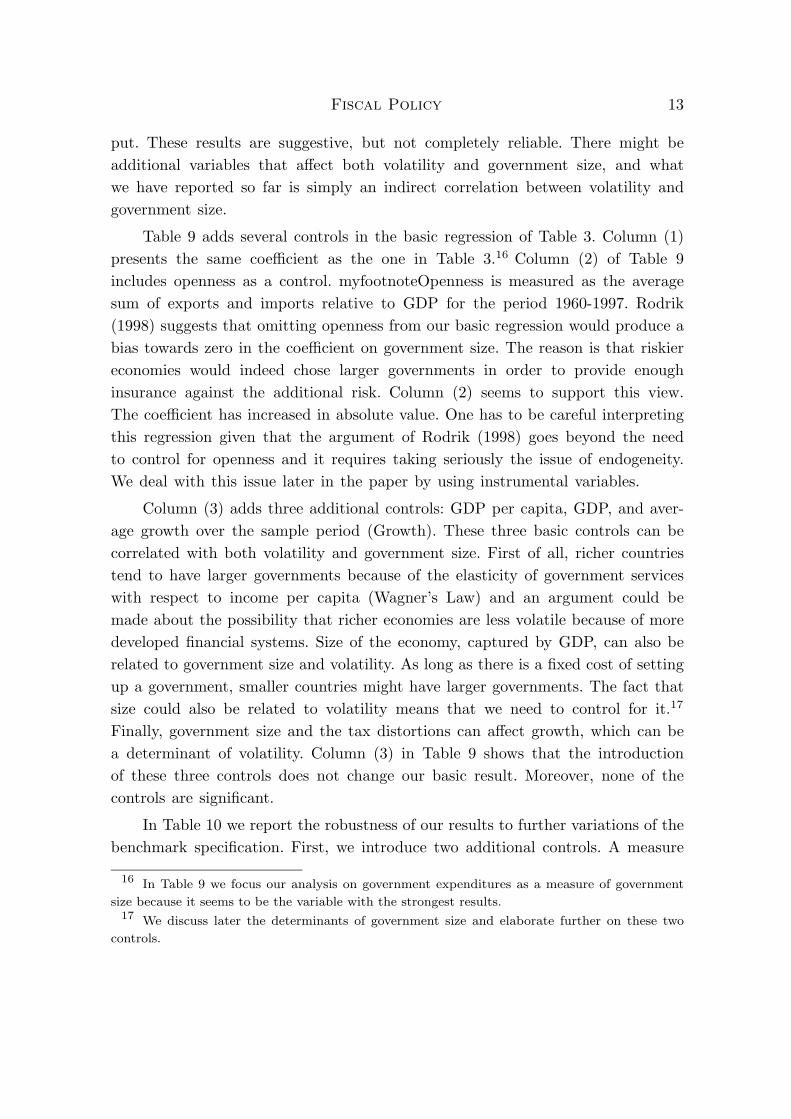
To determine the sources of endogeneity and to be able to create a list ofexogenous instrumental variables, we explore first the determinants of governmentsize. Table 11 reports regressions of government size on openness and several po-litical and economic variables that can serve as instruments. The first columnpresents a Rodrik-type regression of government expenditures on openness, realGDP per capita, dependency ratio in 1990, and urbanization in 1990. The justi-fication for the initial set of explanatory variables is as follows. Openness affectsthe size of the government sector for reasons already discussed in the previoussection. Namely, faced with higher volatility implied by greater openness, house-holds will vote for an increase in the size of the government sector in order to

Fiscal Policy 16

minimize their exposure to risk. Turning now to the GDP per capita, accordingto the Wagner’s Law richer countries can afford larger government sectors becausesome public goods are considered to be income elastic. Finally, the urbanizationrate and the dependency ratio are standard determinants of government spending,as countries with larger non-urban population are expected to face bigger costsin providing public goods and also government spending increases with the risein the ratio of retirees to working-age population. Relative to Rodrik’s regressionwe have slightly changed the time frame with openness being measured as theaverage sum of exports and imports relative to GDP for the period 1960-1969 andgovernment size is the average for 1970-1997. The results are robust to alternativechoices of average openness and average size. Openness enters with the expectedpositive sign and it is statistically significant at better than 1% level.

Table 11. Determinants of Government Size

Dependent Variable: Government Expenditures

(1) (2) (3)

Open6069 0.200 0.167 0.101(3.50) (1.63) (0.98)

GDP per capita 0.286 0.311 0.623

(1.75) (1.73) (2.58)

Dependency 0.453 0.397 0.724

(1.18) (0.95) (1.62)

Urbanization 0.109 0.138 0.017

(0.69) (0.77) (0.09)

GDP - -0.021 -0.011(-0.39) (-0.22)

Presidential - - -0.236(-1.58)

Majoritarian - - -0.132

(-1.36)

Adjusted R2 0.446 0.413 0.476

Sample: 1960-1997.t-statistics in parentheses

All regressions include an intercept.

The second column controls for country size by including real GDP. This re-

Fiscal Policy 17

gression is in the spirit of the work of Alesina and different coauthors (Alesina andWacziarg (1998), Alesina and Spolaore (1997) and Alesina, Spolaore and Wacziarg(1997)) who also argue that the size of government is endogenous and determinedby politico-economic factors. In particular, Alesina and Spolaore (1997) arguethat there are fixed costs in setting up governments. This suggests that smallercountries will have larger governments as percentage of GDP. Alesina, Spolaoreand Wacziarg (1997) provide a theoretical justification for the well-documentednegative correlation between country size and openness: Larger countries can af-ford not to trade with the rest of the world because their market size can ensuresufficiently high productivity. Hence country size is a joint determinant of boththe size of government spending and of the degree of economic openness. Indeed,in a regression controlling for the size of the country the significance of the coef-ficient on openness is much smaller, thereby confirming the conjecture of Alesinaand Wacziarg (1998) that country size might partially account for the correlationbetween openness and government size. Finally, the third column in Table 11 in-cludes two dummy variables suggested by Persson and Tabellini (1998). The firstone controls for the type of the political system – presidential or parliamentary –and takes a value of one for countries with presidential democracies. The seconddummy controls for the type of the electoral system – majoritarian versus propor-tional – and it takes a value of one for countries that have majoritarian elections.Persson and Tabellini (1998) argue that the direct accountability of politicians inpresidential systems increases the competition both among politicians and votersand this implies less spending on every budget item and smaller governments.Furthermore, competition for voters in a majoritarian system targets the swingvoter and creates incentives for more redistribution at the expense of the provisionof public goods. Hence majoritarian systems should be associated with smallerspending on public goods. Both of these variables enter the regression with theexpected sign, albeit both of them are insignificant. Yet, there is a significant im-provement in the fit of the regression from 41.3% to 47.6%. The inclusion of thesevariables further reduces the magnitude and the significance of the coefficient onopenness.20

20 Rodrik (1998) is aware of the fact that his results do not survive in the OECD sampleonce controls for government size are included. Our point here is not to judge the sensitivity

of his results in different samples, but to find an appropriate set of instrumental variables for

government size that is reasonably exogenous and does not suffer from problems associated withweak instruments. Clearly the regressors in column (3) provide one possible list of instrumental

variables.

Fiscal Policy 18

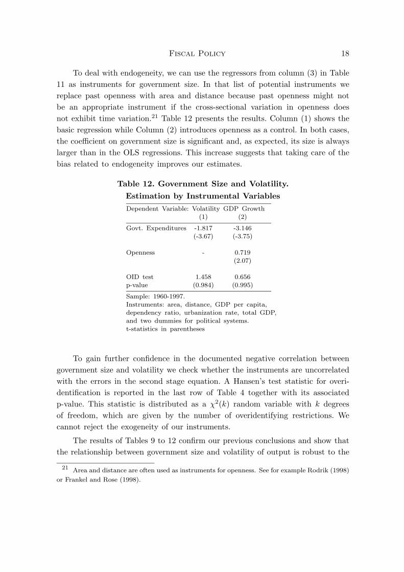
To deal with endogeneity, we can use the regressors from column (3) in Table11 as instruments for government size. In that list of potential instruments wereplace past openness with area and distance because past openness might notbe an appropriate instrument if the cross-sectional variation in openness doesnot exhibit time variation.21 Table 12 presents the results. Column (1) shows thebasic regression while Column (2) introduces openness as a control. In both cases,the coefficient on government size is significant and, as expected, its size is alwayslarger than in the OLS regressions. This increase suggests that taking care of thebias related to endogeneity improves our estimates.

Table 12. Government Size and Volatility.

Estimation by Instrumental Variables

Dependent Variable: Volatility GDP Growth(1) (2)

Govt. Expenditures -1.817 -3.146(-3.67) (-3.75)

Openness - 0.719

(2.07)

OID test 1.458 0.656

p-value (0.984) (0.995)

Sample: 1960-1997.

Instruments: area, distance, GDP per capita,dependency ratio, urbanization rate, total GDP,

and two dummies for political systems.

t-statistics in parentheses

To gain further confidence in the documented negative correlation betweengovernment size and volatility we check whether the instruments are uncorrelatedwith the errors in the second stage equation. A Hansen’s test statistic for overi-dentification is reported in the last row of Table 4 together with its associatedp-value. This statistic is distributed as a χ2(k) random variable with k degreesof freedom, which are given by the number of overidentifying restrictions. Wecannot reject the exogeneity of our instruments.

The results of Tables 9 to 12 confirm our previous conclusions and show thatthe relationship between government size and volatility of output is robust to the

21 Area and distance are often used as instruments for openness. See for example Rodrik (1998)

or Frankel and Rose (1998).

Fiscal Policy 19

inclusion of controls and the correction for possible endogeneity biases.

An additional test for robustness of the relationship between government sizeand volatility can be found in Fatas and Mihov (forthcoming). We present regres-sions similar to the ones above but for US states. Using intranational data hasthe advantage that it is not subject to some of the problems of omitted variablesand endogeneity of the OECD sample. Because US states share many insitutionssuch as labor markets, financial markets, the problem of omitted variables is mini-mized. Moreover, when one looks at measures of government size based on federaltaxes, which are determined at the national level, the results are not subject tothe problems of endogeneity raised by Rodrik (1998). In Fatas and Mihov (forth-coming) we find that across US states, there is a robust negative relationshipbetween measures of government size and volatility of economic fluctuations. Thecoefficient of the regression is larger than the one found in the OECD sample.

3.6 Do Governments Stabilize Output Fluctuations?

The results discussed in the previous sections offer strong support for the viewthat governments stabilize output fluctuations. The robustness across regressionsand samples is a fact that cannot be ignored when looking at business cycleproperties in these economies. The results are very much in line with a Keynesianview of automatic stabilizers, although there are still unanswered questions aboutthe mechanisms that are behind the results. Our attempts to uncover what isbehind government size have not been that successful. Marginal tax rates, cyclicalelasticities of fiscal variables, components of the budget related to business cycles(such as transfers) are dominated in our regressions by the simplest measureof fiscal policy: government size. Whether this is simply due to the difficulty ofmeasuring automatic stabilizers properly has is an answered question at this pointand will have to be addressed by future research.

4. Discretionary Fiscal Policy

The goal of this section is to study how the economy reacts to various shiftsin fiscal policy. The first issue to be resolved in an empirical study of fiscal policyis what indicator to use as a measure of policy stance. A notable ready-madecandidate for this role is the budget deficit - either the deficit in the overall fi-nancial balance or in the primary balance. There are, however, several well-knownproblems with this measure that make it a poor indicator of discretionary fiscal

Fiscal Policy 20

policy. The deficit captures both exogenous policy shifts as well as automaticreaction of fiscal variables to the state of the economy thus confounding policyeffects and endogenous economic fluctuations. Furthermore, even when changesin the deficit reflect purely discretionary policy decisions, it is obvious that thesource of the change – whether it is a revenue adjustment or a change in govern-ment spending – is important for the subsequent reaction of the private sector,as Blanchard and Perotti (1999) argue. Finally, from a theoretical point of viewchanges in government consumption might have a different macroeconomic effectthan changes in investment or increases in transfers, which requires looking atthe different components of the budget.22

The first criticism – the endogenous nature of the budget balance – canbe handled by removing the reactive components, taxes and transfers, from thefiscal balance thus concentrating only on the autonomous components of spending.Admittedly this is a crude way of adjustment that might throw away importantand interesting information. An alternative method is to construct a ‘cyclically-adjusted’ fiscal balance as is the current practice at the IMF and the OECD.The adjustment is carried out by establishing a benchmark cyclical indicator (anoutput gap, for example) and relating the deficit to the state of the cycle relativeto the benchmark.23 An interesting contribution to this literature is a paper byBlanchard (1993). He also argues that an indicator of discretionary fiscal policymust be relative in nature. The procedure outlined in his paper requires selectinga pre-specified benchmark and estimating elasticities of the different componentsof the budget with respect to a representative set of macroeconomic variables. Theresponse of the budget deficit to current economic conditions is then constructedby using the estimated elasticities. The difference between this value and theactual budget deficit is a measure of discretionary fiscal policy. The originalrecommendation is to use unemployment, inflation, and interest rates in theconstruction of the induced changes in the budget balance. Indeed, a version ofthis indicator has been recently used in a paper by Alesina and Perotti (1995). Intheir study of fiscal consolidations in OECD countries they construct an indicatorof fiscal policy by using the current rate of unemployment as the driving variablefor transfers and taxes. Here we extend their work by taking a slightly agnosticbut more general approach. First, we use GDP instead of unemployment, but we

22 To address this last issue we report the effects of disaggregated fiscal policy variables – taxes,

transfers, spending on wages, investment and non-wage spending.23 See Alesina and Perotti (1995) for a discussion and criticism of these measures.

Fiscal Policy 21

also include a measure of the price level and interest rates. Second, we use vectorautoregressions (VAR) to summarize the basic comovements in the data and toextract the indicator of fiscal policy stance.

Both Blanchard (1993) and Alesina and Perotti (1995) argue that one ofthe desirable features of an indicator of discretionary fiscal policy is simplicity.Clearly, our measure is based on a slightly more complicated model than theirsuggestions, but the trade-off of simplicity is precision and the number of assump-tions underlying the construction of the indicator. In this paper, we attempt tosee how the introduction of more variables and imposing a less restrictive econo-metric structure improves the properties of the fiscal policy indicator.

4.1 The Data and the VAR Framework

Throughout this section we use US data to measure the effects of discre-tionary fiscal policy.24 The main reason why we focus on the US is the availabilityof good quarterly data on fiscal variables. Also, there is a established literaturethat has looked at the US economy and we would like to compare our results tothose obtained in these other papers.

Our baseline VAR contains logarithm of private output, logarithm of theimplicit GDP deflator, ratio of primary deficit to output and nominal T-billrate. Based on the Akaike information criterion we select 4 lags (values from1 to 12 have been tried for the lag length). This composition of the vector ofendogenous variables must be regarded as the minimal set of macroeconomicvariables necessary for the construction of an indicator of fiscal policy.

In addition to the regular assumptions underlying every vector autoregres-sion, we impose restrictions on the contemporaneous relationship between macroe-conomic variables. Our argument follows the semi-structural VAR literature.25

This framework is summarized by the following two equations:

Yt =k∑i=0

BiYt−i +k∑i=0

Cifpt−i +Ayvyt (2)

24 Data is taken from the NIPA files at quarterly frequency and the averaged quarterly T-bill

rate. The sample is from 1960:1 to 1996:4.25 See Bernanke and Blinder (1992) and Bernanke and Mihov (1998) for an application of semi-

structural VARs to the study of monetary policy. The framework used in this section is discussed

extensively by Bernanke and Mihov (1998).

Fiscal Policy 22

fpt =k∑i=0

DiYt−i +k∑i=0

gifpt−i + vfpt (3)

For the study of fiscal policy, vector Y represents the set of macroeconomicvariables necessary for estimating the induced changes in the budget balance.fp is a measure of fiscal policy stance.26 This set of equations is unrestrictedand the fiscal policy shocks denoted by vfp cannot be recovered without furtherassumptions. Here we follow Leeper, Sims and Zha (1996) in partitioning thevector of endogenous variables in three blocks: (1) A subset of vector Y contains“sluggish” private sector variables, which do not respond contemporaneously toshifts in taxes and transfers or to the primary deficit in the first estimation below.They do react, however, to changes in government spending. In this vector weinclude output and prices and we impose the restrictions on a combination ofC0, B0, and Ay to ensure no response to tax and transfer shocks or to shocksto other Y variables; (2) The rest of vector Y contains auction prices whichrespond immediately to any change in the economic environment. No restrictionis imposed for these equations; (3) The fiscal policy equation is restricted notto respond to financial markets shocks within a quarter, but taxes and transfersreact to the current state of the economy, while generic spending components likewage spending, investment and non-wage spending do not react immediately tomacroeconomic conditions.

An alternative to the VAR approach is advocated by Edelberg, Eichenbaumand Fisher (1998) and Burnside, Eichenbaum and Fisher (1999). They argueagainst using VAR-based innovations in fiscal variables as measures of policy shiftsand propose a study based on dummies for three episodes of military build-ups.These episodes have been isolated by Ramey and Shapiro (1998) and include theKorean War, 1950:3, the Vietnam War, 1965:1, and the Carter-Reagan defensebuild-up, 1980:1. The effects of fiscal policy are calculated as the response ofthe economy to an innovation in the dummy for the Ramey-Shapiro episodes.The analysis based on the Ramey-Shapiro episodes produces noticably differentresults from the VAR, as we document in Fatas and Mihov (2000). We find thismethodology interesting, but certainly in need of a closer analysis because thethree episodes differ significantly in their implications for the persistence and the

26 Here we make the Bernanke-Blinder assumption that a scalar measure of policy stance is

available. In our future work, we plan to extend this analysis along the lines of Bernanke andMihov (1988) with the measure of fiscal policy being recovered from a vector of relevant fiscal

policy variables.

Fiscal Policy 23

magnitude of the increase in government spending.27

4.2 The Indicator of Policy Stance

The assumptions listed in the previous paragraph provide a simple way ofestimating our baseline VAR and extracting a measure of fiscal policy. Afterestimating the reduced form version of equations (2) and (3) we orthogonalizethe residuals from the fiscal policy equation to contemporaneous movements inoutput and prices. This orthogonalized residual is our measure of unanticipatedfiscal policy shifts. Figure 3 presents a smoothed version of this measure in graphicform.28 Positive values on the graph indicate increases in the primary deficit tooutput ratio.


We can discern on this graph some of the major changes in fiscal policyin the US: The Kennedy-Johnson tax cut in 1964, the Reagan tax cut of 1981,and the Gulf war, among others. Interpretation, however, along these lines isa little bit stretched because most of these events were anticipated as of theprevious quarter. The VAR results, however, do suggest that these effects werenot fully anticipated. Ideally we would like to construct a measure which takesinto account also anticipated policy, but this will require making assumptionsthat are too much model-specific. At this point we explore what conclusions wecan draw from a minimal set of assumptions, which is consistent with the viewtaken by the researchers on macroeconomic effects of monetary policy.

This indicator of fiscal policy stance turns out to be very highly correlatedwith the measure based on Blanchard’s (1993) suggestions and constructed byAlesina and Perotti (1995). We have used their methodology to calculate a quar-terly version of their indicator and we find that the correlation of the indicatoron Figure 3 with their measure is 0.82. This result is quite remarkable given thedifferences in methodology. Fundamentally, of course, the theoretical justification

27 Another issue that our methodology does not capture is the possibility of non-linearities inthe effects of fiscal policy shocks. These non-linearities can be, for example, related to the level

of government debt, as suggested by Giavazzi and Pagano (1990). We think that in the case of

the US this might be less of an issue but, certainly, if we were to apply this methodology to other

countries, one would need to allow for these non-linearities.28 We have smoothed the series by a centered seven-quarter moving average of fiscal policy

shocks to improve readability of the measure.

Fiscal Policy 24

of our approach follows the same logic as that of Blanchard (1993). It is, how-ever, quite surprising that the dramatic improvement in the fit in our regressionstranslates only in marginal improvement in the measure. We take, however, thisresult as a confirmation of our general strategy of extending the set of macroeco-nomic variables influencing the budget and of relaxing the lag length restrictionsin Alesina and Perotti (1995).

4.3 Responses to Fiscal Policy Shocks

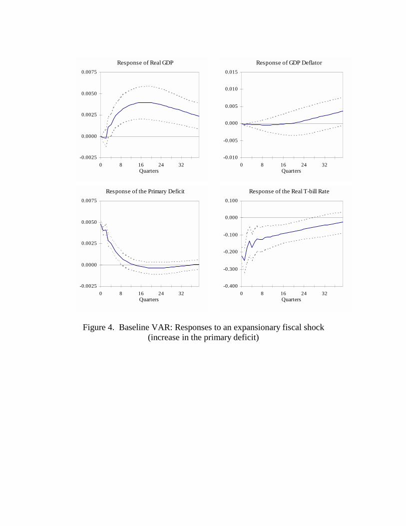
We now go to the study of the economic effects of changes in fiscal policy.First, we use our baseline VAR. Figure 4 shows the responses of the endogenousvariables to a one standard deviation shock in the primary deficit to output ratio.The impulse responses are reported for a horizon of ten years with one-standard-deviation error bands calculated with Monte Carlo integration methods with 500replications. The baseline vector autoregression consists of the following variables:(GDPt, PGDPt, PDeft, Rbillt), where GDPt is real GDP, PGDPt is the GDPdeflator,PDeft is the ratio of the primary deficit to nominal GDP,RBillt is theex post real interest rate on three months Treasury bills.29


There is a strong and persistent reaction of output to a fiscal shock. Thispersistence is somewhat puzzling given that the primary deficit goes back toits baseline trend less than two years after the shocks. This result is robust tochanges in lag structure, estimation period, or inclusion of other variables inthe system. Clearly, the increase in output must lead to by construction to adecline in the deficit by increasing the denominator of the fiscal variable. But thedynamics of the deficit cannot be explained purely with this logic: Using the realprimary deficit instead of the ratio to output leads to the same result. Anotherpossible channel is working through the tax receipts. To justify on these groundsthe closing of the deficit one has to use the explanatory power of the progressivityof taxes or of a Laffer curve relationship. We will return to this issue later.

The response of the price level is never statistically significant, while interestrates move in a counterintuitive way: Contemporaneously with the increase in theprimary deficit, interest rates decline by about twenty-five basis points and thereturn to trend is very slow. It turns out that the result is not very robust and

29 The data source is the DRI Basic Economics Database and the University of Virginia NIPA

web site.

Fiscal Policy 25

in VARs that account more carefully for the composition of the fiscal shock, thedynamics of interest rates exhibit the expected behavior – expansionary policyincreases both real and nominal rates.

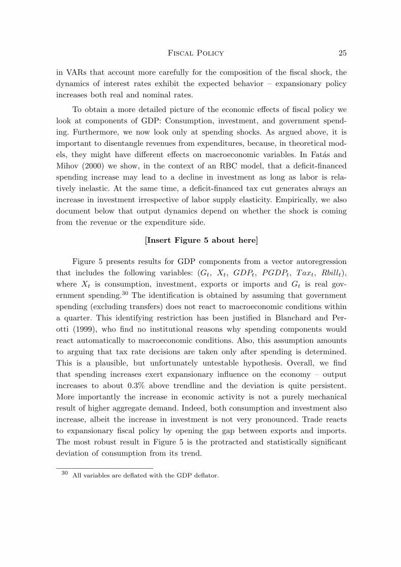
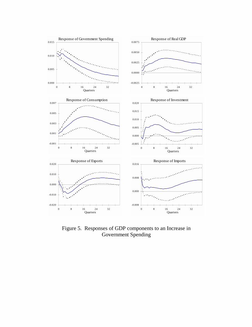
To obtain a more detailed picture of the economic effects of fiscal policy welook at components of GDP: Consumption, investment, and government spend-ing. Furthermore, we now look only at spending shocks. As argued above, it isimportant to disentangle revenues from expenditures, because, in theoretical mod-els, they might have different effects on macroeconomic variables. In Fatas andMihov (2000) we show, in the context of an RBC model, that a deficit-financedspending increase may lead to a decline in investment as long as labor is rela-tively inelastic. At the same time, a deficit-financed tax cut generates always anincrease in investment irrespective of labor supply elasticity. Empirically, we alsodocument below that output dynamics depend on whether the shock is comingfrom the revenue or the expenditure side.


Figure 5 presents results for GDP components from a vector autoregressionthat includes the following variables: (Gt, Xt, GDPt, PGDPt, Taxt, Rbillt),where Xt is consumption, investment, exports or imports and Gt is real gov-ernment spending.30 The identification is obtained by assuming that governmentspending (excluding transfers) does not react to macroeconomic conditions withina quarter. This identifying restriction has been justified in Blanchard and Per-otti (1999), who find no institutional reasons why spending components wouldreact automatically to macroeconomic conditions. Also, this assumption amountsto arguing that tax rate decisions are taken only after spending is determined.This is a plausible, but unfortunately untestable hypothesis. Overall, we findthat spending increases exert expansionary influence on the economy – outputincreases to about 0.3% above trendline and the deviation is quite persistent.More importantly the increase in economic activity is not a purely mechanicalresult of higher aggregate demand. Indeed, both consumption and investment alsoincrease, albeit the increase in investment is not very pronounced. Trade reactsto expansionary fiscal policy by opening the gap between exports and imports.The most robust result in Figure 5 is the protracted and statistically significantdeviation of consumption from its trend.

30 All variables are deflated with the GDP deflator.

Fiscal Policy 26

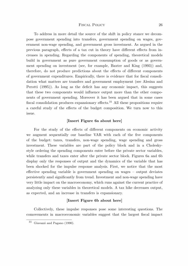
To address in more detail the source of the shift in policy stance we decom-pose government spending into transfers, government spending on wages, gov-ernment non-wage spending, and government gross investment. As argued in theprevious paragraph, effects of a tax cut in theory have different effects from in-creases in spending. Regarding the components of spending, theoretical modelsbuild in government as pure government consumption of goods or as govern-ment spending on investment (see, for example, Baxter and King (1993)) and,therefore, do not produce predictions about the effects of different componentsof government expenditures. Empirically, there is evidence that for fiscal consoli-dation what matters are transfers and government employment (see Alesina andPerotti (1995)). As long as the deficit has any economic impact, this suggeststhat these two components would influence output more than the other compo-nents of government spending. Moreover it has been argued that in some casesfiscal consolidation produces expansionary effects.31 All these propositions requirea careful study of the effects of the budget composition. We turn now to thisissue.

[Insert Figure 6a about here]

For the study of the effects of different components on economic activitywe augment sequentially our baseline VAR with each of the five componentsof the budget: taxes, transfers, non-wage spending, wage spending and grossinvestment. These variables are part of the policy block and in a Cholesky-style ordering the spending components enter before the private sector variables,while transfers and taxes enter after the private sector block. Figures 6a and 6bdisplay only the responses of output and the dynamics of the variable that hasbeen shocked for the impulse response analysis. First, we notice that the mosteffective spending variable is government spending on wages – output deviatespersistently amd significantly from trend. Investment and non-wage spending havevery little impact on the macroeconomy, which runs against the current practice ofanalyzing only these variables in theoretical models. A tax hike decreases output,as expected, and an increase in transfers is expansionary.

[Insert Figure 6b about here]

Collectively, these impulse responses pose some interesting questions. Thecomovements in macroeconomic variables suggest that the largest fiscal impact

31 Giavazzi and Pagano (1990).

Fiscal Policy 27

on the economy comes from transfers, taxes, and government employment. The-oretical models, however, build in government as pure consumption of goods andinvestment. We view our results as a call for introducing government employ-ment in dynamic stochastic general equilibrium models explicitly and for buildingmodels with heterogeneous agents to account for the effects of transfers on eco-nomic activity. Furthermore, the results on the GDP components suggests thatexpansionary fiscal policy leads to an increase in consumption. This result, albeitconsistent with a textbook presentation of the Keynesian cross, flies in the face ofmost general equilibrium models. In Fatas and Mihov (2000) we document thatunder plausible values of calibration parameters, the baseline real business cyclemodel and its modifications lead inevitably to a decline in private consumptionwhen government spending increases. Certain failures of the Ricardian equivalencecould generate the positive effect of spending on consumption, and we expect thatfuture research will address this issue in detail.

5.- Conclusions

This paper studies the effects of fiscal policy on economic activity. The firstpart of the paper looks at the effects of automatic stabilizers. In a sample of 20OECD economies, we find that large governments are associated with less volatilebusiness cycles. This effect cannot be directly associated to any specific componentof government expenditures or revenues. The stabilizing effects of fiscal policy alsocarry over to the private sector. Large governments are negatively correlated withthe volatility of private GDP.

We look for economic mechanisms that can explain the negative correla-tion between government size and macroeconomic stability by introducing directmeasures of automatic stabilzers. We construct a quantitative measure of the au-tomatic response of fiscal policy to output fluctuations but we find that it cannotexplain the correlation between size of government and GDP volatility. Marginaltax rates can explain part of the correlation but given the high collinearity be-tween marginal and average tax rates is difficult to separate both effects.

We check for the robustness of our results by introducing a long list ofcontrols and by taking into consideration the endogeneity of government size.In all cases, our main result, that large governments stabilize business cycles, ispresent.

In the second part of the paper we construct a measure of discretionay policy.

Fiscal Policy 28

Our measure uses VAR techniques similar to the ones used in the studies ofmonetary policy. We find that our estimate of discretionary fiscal policy is highlycorrelated with a constructed measure following the suggestions of Blanchard(1993) and applied by Alesina and Perotti (1995).

When we calculate the reponse of economic activity to changes in fiscal policywe find that there is a strong, positive and persistent impact of fiscal expansionson economic activity.

We disaggregate fiscal policy into different components and we find thatchanges in taxes, transfers and government employment are the most effectivetools of fiscal policy. Our results are difficult to compare with calibrated stochas-tic general equilibrium models because, in general, these models do not take intoconsideration the determinants of different components of government expendi-tures and taxes.

Overall, our results suggest that further research is needed to build modelsof fiscal policy that can account for the facts presented in this paper. Explicitlymodeling government employment might provide an avenue for explaining someof these facts.

Fiscal Policy 29

6.- References

Alesina, Alberto and Roberto Perotti (1996). “Fiscal Adjustment”. EconomicPolicy, 21.

Asdrubali, Pierfederico, Bent E. Sorensen and Oved Yosha (1996). “Channelsof Interstate Risk Sharing: United States 1963-1990”. Quarterly Journal of Eco-nomics, 111(4).

Baxter, Marianne and Robert G. King (1993). “Fiscal Policy in General Equilib-rium”. American Economic Review, 83(3).

Bayoumi, Tamim and Paul R.Masson (1996), “Fiscal Flows in the United Statesand Canada: Lessons for Monetary Union in Europe”. European Economic Review,39.

Bernanke, Ben and Alan Blinder (1992). “The Federal Funds Rate and the Chan-nels of Monetary Transmission”, American Economic Review,

Bernanke, Ben and Ilian Mihov (1998). “Measuring Monetary Policy”, QuarterlyJournal of Economics,

Blanchard, Olivier (1993). “Suggestions for a New Set of Fiscal Indicators”, inH.A.A. Verbon and F.A.A.M. van Winden (editors), The New Political Economyof Government Debt, Elsevier Science Publishers.

Christiano, Lawrence J. (1994) “A reexamination of the Theory of AutomaticStabilizers”. Carnegie-Rochester Conference Series on Public Policy, 20.

Cohen, Darrel and Glenn Follette (1999) “The automatic stabilizers: quietlydoing their thing”. Federal Reserve Board, Working Paper.

Cochrane, John (1998). “What do the VARs mean? Measuring the output effectsof monetary policy”, Journal of Monetary Economics, (41)2.

Eichengreen, Barry and Charles Wyplosz (1998). “The Stability Pact: More thana Minor Nuisance?” Economic Policy, 26.

Fatas, Antonio (1998). “Does EMU Need a Fiscal Federation?” Economic Policy,26.

Fatas, Antonio and Ilian Mihov (forthcoming). “Government Size and AutomaticStabilizers” Journal of International Economics, .

Fatas, Antonio and Ilian Mihov (2000). “The Macroeconomic Effects of FiscalPolicy”, mimeo, INSEAD.

Fiscal Policy 30

Galı, Jordi (1994), “Government Size and Macroeconomic Stability”. EuropeanEconomic Review, 38.

Giavazzi, Francesco and Marco Pagano (1990). “Can Severe Fiscal AdjustmentsBe Expansionary?”, NBER Macroeconomics Annual, MIT Press.

Leeper, Eric, Christopher Sims and Tao Zha (1996). “What Does Monetary PolicyDo?”, Brookings Papers on Economic Activity, 2.

McKee, Michael J., Jacob J.C. Visser and Peter G. Saunders (1986). “MarginalTax Rates and the use of Labor and Capital in OECD Countries” OECD Eco-nomic Studies, 7.

Sachs, Jeffrey and Xavier Sala-i-Martin (1992), “Fiscal Federalism and OptimumCurrency Areas: Evidence from Europe and the United States”. In MatthewCanzoneri, Vittorio Grilli, and Paul Masson, eds. Establishing a Central Bank:Issues in Europe and Lessons from the U.S.

Sims, Christopher (1980), “Macroeconomics and Reality”, Econometrica, 48.

von Hagen, Jurgen (1992). “Fiscal Arrangements in a Monetary Union: Evidencefrom the US”. In Don Fair and Christian de Boissieux, eds., Fiscal Policy, Taxes,and the Financial System in an Increasingly Integrated Europe. Kluwer AcademicPublishers.

Fiscal Policy 31

7.- Appendix

DATA SOURCES. All OECD data from the OECD economic outlook. Originalcodes and definition of constructed variables.

CGNW= Government Consumption (non-wages)CGW = Government Consumption (wages)IG = Government Gross InvestmentTSUB = SubsidiesSSPG = Social Security Transfers Paid by the GovernmentTRPG = Other Transfers Paid by the GovernmentTY = Direct TaxesTIND = Indirect TaxesTRRG = Transfers Received by GovernmentKTRRG = Capital Transfers Received by GovernmentRESTG = Other capital TransfersGNINTP = Net Interest Payments on Government DebtYPEPG = Income Property Paid by GovernmentYPERG = Income Property Received by GovernmentCFKG = Consumption of Government Fixed CapitalNLG = Net Lending by GovernmentCPAA = Private ConsumptionGDP = Gross Domestic ProductPGDP = Deflator of GDPYDH = Household Disposable IncomeEXPENDTURES = CGNW + CGW + IG + TSUB + SSPG + TRPGREVENUES = SSRG + TY + TIND + TRRGTRANSFERS = TSUB + SSPG + TRPGPRIMARY DEFICIT = EXPEND - REVEN - KTRRG - RESTG -

- GNINTP + YPEPG - YPERG - CFKG

All US quartely data from NIPA. Same definitions as above apply.

AUT

SWI

FIN

SWE

NOR

AUS

JAP

CANUS

POR

GRE

SPA

DENIRE

UKBEL

NET

ITA

FRAGER

1.4

1.9

2.4

2.9

3.4

3.9

20 25 30 35 40 45 50

Government Size (Expenditures/GDP)

Vol

atili

ty G

DP

Figure 1. Government Size and Output Volatility

AUT

SWI

FIN

SWE

NOR

AUS

JAP

CAN

US

POR

GRE

SPA

DENIRE UK

BEL

NET

ITA

FRAGER

1.4

1.9

2.4

2.9

3.4

3.9

4.4

20 25 30 35 40 45 50

Government Size (Expenditures/GDP)

Vol

atili

ty P

rivat

e O

utpu

Figure 2. Government Size and Volatility of Private Output

Measure of Unanticipated Fiscal Policy

-0.005

-0.003

-0.001

0.001

0.003

0.005

62:0

1

64:0

1

66:0

1

68:0

1

70:0

1

72:0

1

74:0

1

76:0

1

78:0

1

80:0

1

82:0

1

84:0

1

86:0

1

88:0

1

90:0

1

92:0

1

94:0

1

96:0

1

Figure 3. Measure of unanticipated fiscal policy (smoothed)

(Quarterly VAR, 1961:1 - 1996:4)

Response of Real GDP

-0.0025

0.0000

0.0025

0.0050

0.0075

0 8 16 24 32Quarters

Response of GDP Deflator

-0.010

-0.005

0.000

0.005

0.010

0.015


Response of the Primary Deficit

-0.0025

0.0000

0.0025

0.0050

0.0075


Response of the Real T-bill Rate

-0.400

-0.300

-0.200

-0.100

0.000

0.100


Figure 4. Baseline VAR: Responses to an expansionary fiscal shock (increase in the primary deficit)

Response of Government Spending

0.000

0.005

0.010

0.015


Response of Real GDP

-0.0025

0.0000

0.0025

0.0050

0.0075


Response of Consumption

-0.001

0.001

0.003

0.005

0.007


Response of Investment

-0.005

0.000

0.005

0.010

0.015

0.020


Response of Exports

-0.020

-0.010

0.000

0.010

0.020


Response of Imports

-0.008

0.000

0.008

0.016


Figure 5. Responses of GDP components to an Increase in Government Spending

Shock to Government Non-Wage Spending

Response of Non-wage Spending

-0.010

0.000

0.010

0.020

0.030


Response of Output

-0.005

0.000

0.005

0.010


Shock to Wage Spending

Response of Government Wages

-0.010

0.000

0.010

0.020


Response of Output

-0.005

0.000

0.005

0.010


Shock to Government Investment

Response of Government Investment

-0.010

0.000

0.010

0.020

0.030

0.040


Response of Output

-0.005

0.000

0.005

0.010


Figure 6a. Responses of GDP and budget components to fiscal shocks

Shock to Transfers

Response of Transfers

-0.010

-0.005

0.000

0.005

0.010

0.015

0.020


Response of Output

-0.002

0.000

0.002

0.004

0.006


Shock to Taxes

Response of Taxes

-0.015

-0.010

-0.005

0.000

0.005

0.010

0.015


Response of Output

-0.009

-0.006

-0.003

0.000

0.003


Figure 6b. Responses of GDP and budget components to fiscal shocks

Documents

Fiscal Policy and Business Cycles: An Empirical Investigationfaculty.insead.edu/fatas/myc.pdf · Fiscal Policy and Business Cycles: An Empirical Investigation ... positive, do countries