Embed Size (px)
Citation preview

i
FISCAL AND MONETARY POLICY INTERACTIONS IN THE
NIGERIAN ECONOMY- A NEW KEYNESIAN APPROACH
By
OYE, QUEEN ESTHER
Matriculation Number: 04AF00562
NOVEMBER, 2018

ii
FISCAL AND MONETARY POLICY INTERACTIONS IN THE
NIGERIAN ECONOMY- A NEW KEYNESIAN APPROACH
By
OYE, QUEEN ESTHER
Matriculation Number: 04AF00562
B.Sc, M.Sc Covenant University, Ota
A THESIS SUBMITTED TO THE SCHOOL OF POSTGRADUATE IN
PARTIAL FULFILMENT FOR THE AWARD OF THE DEGREE OF
DOCTOR OF PHILOSOPHY IN THE DEPARTMENT OF ECONOMICS
AND DEVELOPMENT STUDIES, COLLEGE OF BUSINESS AND
SOCIAL SCIENCES, COVENANT UNIVERSITY.
NOVEMBER, 2018

iii

iv

v

vi
DEDICATION
This thesis is dedicated to the Almighty God, my Father, the source of wisdom and help. His
son, the beginning and end; and the Holy Spirit who inspired and taught me. I am grateful.

vii
ACKNOWLEDGEMENTS
I give thanks to my Heavenly Father, who is the God Almighty for the successful completion
of this thesis. I express my appreciation to several individuals that have contributed directly or
indirectly, through the diverse phases of the research and writing of this dissertation. My
profound gratitude goes to the Chancellor and Chairman of the Board of Regents, Covenant
University, Dr. David O. Oyedepo, for the conducive spiritual and mentorship pedestal, which
facilitated the success of this research work. I acknowledge the Vice-Chancellor Prof. AAA
Atayero, the Deputy Vice-Chancellor, Prof. A. Williams, the Registrar, Dr. O. Oludayo and all
other members of the management team of Covenant University for their commitment to
Vision 10:2022 and for providing an academic-enabling environment to learn, research and
write this thesis.
I acknowledge the meticulous leadership and guidance of the Dean of Postgraduate school,
Prof. A.H. Adebayo, the Dean of Business and Social Sciences, Prof. Philip O. Alege and
everyone that served as the College and Postgraduate school representative at my College-
level presentations, including Prof. U. Uwuigbe, Dr. H. Okodua and Prof. I.S. Afolabi. I
recognise your valuable contributions and efforts towards improving the quality of the thesis.
Thank you very much sirs.
I particularly acknowledge my Supervisor, Prof. Philip O. Alege, for insisting on nothing but
high-quality research. He also took out time to read, correct, re-read and give helpful feedbacks
and instructions at each stage of the research writing. I also appreciate his role in mentoring
me into the framework of Dynamic Stochastic General Equilibrium models. My profound
appreciation also goes to my Co-Supervisor, Prof. A. Olomola for his good wishes,
encouragement and constructive criticisms that challenged my thinking and strengthened the
quality of this work. I also acknowledge erudite Professors in the Department of Economics
and Development Studies, including Prof. O. Olurinola, Prof. G. Oni, Prof. S. Edo and Prof.
E. Osabuohien who tirelessly read, corrected and offered helpful comments, which motivated
me to reason and write better. I also appreciate the encouragement that I received from the
Head of Department, Economics and Development Studies, Dr. D. Azuh. I am grateful to you
sirs.

viii
I express my thanks to mentors and colleagues in the Department of Economics and
Development Studies: Doctors H. Okodua, E. Bowale, M. Oladosu, O. Gershon, B. Ewetan,
E. Oduntan, A. Matthew, E. Urhie and others. God bless you all for your prayers, advice,
constructive feedbacks and contributions at the various departmental and college presentation
of this work. In addition, I acknowledge Dr. A. Adegboye of the Department of Economics,
Obafemi Awolowo University whose thesis tremendously aided my understanding of DSGE
modelling. I also recognise the Dynare Forum moderated by Johannes Pfeifer, Michel Julliard,
Stephane Adjemian and Sebastien Villemot. They helped to address bugging simulation and
estimation questions.
My special gratitude goes to my dear parents, Rev. and Pastor (Mrs.) B. Oluwatimiro for their
prayers, financial and moral support all through the years of academic pursuit. I would also not
fail to specially acknowledge my husband, Gbenga Oye and my children: EriOluwa and
IbukunOluwa. Thank you for all that you are to me in God. I deeply appreciate your love,
patience, prayers, support and sacrifices you made in the course of the Ph.D programme. I love
you all.

ix
TABLE OF CONTENTS Page
Cover Page i
Title Page ii
Acceptance iii
Declaration iv
Certification v
Dedication vi
Acknowledgments vii
Table of Contents ix
List of Tables xiii
List of Figures xv
List of Abbreviations xvi
List of Appendices xvii
Abstract xviii
CHAPTEONE: INTRODUCTION……………………...………………..….…….. 1
1.1 Background of the Study…………………..……………....………………………....…… 1
1.2 Statement of Research Problem………………………..…………………………….…… 5
1.3 Research Questions……………………………………..…………………….……..…..... 7
1.4 Research Objectives…………………………………………………………...….…....… 7
1.5 Research Hypotheses………………………………………….……...………..….….…... 7
1.6 Scope of the Study………………………………………………..……………….…….... 8
1.7 Significance of study……………………………………………..…………..…….…..…. 8
1.8 Method of Analysis………………………………………………….....…..…………..…. 9
1.9 Outline of the Study…………………………………………..…….….…………………. 9
CHAPTER TWO: LITERATURE REVIEW……………………….…..……….. 10
2.1 Review of Definitional Issues ………………….…………..………...…..……….......… 10
2.2 Theoretical Review of the Literature...…………………………..………….………...…. 12
2.2.1 Macroeconomic Theories………...…………………………………………………… 12

x
2.2.2 Models of Fiscal and Monetary Policy Interactions ……………………….…….……. 14
2.3 Methodological Review…………………………………..……………….…….…...…. 20
2.3.1 A-theoretic Statistical Methods ……………………………………………....……..… 20
2.3.2 Game Theoretic Models……………………………..…………………….……….….. 23
2.3.3 Dynamic General Equilibrium Methods………………………...…………….………. 26
2.4 Estimation Techniques for NK DSGE models ………………………………….…...….. 35
2.5 Empirical Review……………..………………………………..……….........….…..…. 38
2.5.1 Empirical Evidence from United States and Europe …………….…..………...…….... 38
2.5.2 Empirical Evidence from Asia…………..……………………….…….……………… 41
2.5.3 Empirical Evidence from Latin America………..……………….………………...….. 43
2.5.4 Empirical Evidence from Africa………..………………….………………………….. 44
2.5.5 Empirical Evidence from Nigeria…………..………………….……………………… 45
2.5.6 Empirical Nature of Fiscal and Monetary Policy Interactions.…...….…………..……. 46
2.5.7 Trend in the Empirical Literature………………………………………..…..…..…….. 48
2.6 Summary of Identified Gaps………………………...…………..…………...……...….. 60
CHAPTER THREE: STYLISED FACTS …......………………………..….….… 62
3.1 Structure of the Nigerian Economy…………………………………...…..……....……... 62
3.2 Monetary and Fiscal Policy in the Nigerian Economy…………...……..………..…..… 66
3.2.1 Monetary Policy in Nigeria……………………………………..….………………….. 66
3.2.2 Fiscal Policy in Nigeria……………………………..…………….…………………… 68
3.2.3 Monetary and Fiscal Policy Coordination in Nigeria…………………..…..………….. 74
3.3 Trend Analysis on Fiscal and Monetary Policy in Nigeria ………………………...….. 75
3.4 Business Cycle Facts……………………………………………………..………….…... 86
3.5 Empirical Facts on Alternative Assumptions……………………………..……………... 89
3.6 Summary of Key Issues………………………………………………….....…………… 94

xi
CHAPTER FOUR: METHODOLOGY …………………………...……….…….. 95
4.1 Theoretical Framework …………………..………………….…………………..…...…. 95
4.1.1 The New Keynesian Macro-Economic Model…...………...…………..……...………. 95
4.2 The Research Method………………………..………………………….……...……… 100
4.2.1 An Open Economy New Keynesian DSGE Model for Nigeria ………..…...………... 101
4.2.2 Solving and Estimating the Open Economy NK DSGE model…..……..……….….... 130
4.2.3 System of Equations to be estimated ………………………..………..……...………. 132
4.2.4 Data Sources and Measurements…………………………..………....……………… 142
4.3 Optimal Fiscal and Monetary Policy ………………………….…..………..…………. 143
4.3.1 Ramsey Policy……………………………………………….……………………… 144
4.3.2 Discretionary Policy……………………………………....…………………………. 144
CHAPTER FIVE: RESULTS AND DISCUSSION ………………...…….…….. 146
5. 1 Presentation of Results…………………………………………..…...…..………….… 146
5.1.1 Parameter Estimates of the DSGE Model …………………..….…..….…….….…… 147
5.1.2 Impulse Response Analysis…………………………………..……...……….….….. 153
5.1.3 Variance Decomposition ……………..………………….…….…………….……… 157
5.2 Model Diagnostic Testing……………..………………………..……………………. 159
5.2.1 Stability of the Model………………………..………………...…………………….. 159
5.2.2 Identification of the Parameter Estimates………..………...…..……………….……. 160
5.2.3 Mode Check …………………………………..…………….….……………....….... 162
5.2.4 Univariate Convergence Statistics……………………………….…………….….… 165
5.2.5 Multivariate Convergence Diagnostic……………………….…………………...….. 166
5.2.6 Historical and Smoothed variables………………………………..……...…….....…. 167
5.2.7 Smoothed Shocks …………………………………………...…….……..………..… 168
5.3 Nature of Fiscal and Monetary Policy Interactions……….……..……...……………… 169
xii
5.4 Optimal Fiscal and Monetary Policy………………………..….………..……….……. 173
5.5 Implications of Findings …………………………………..……….……..……….….. 175
CHAPTER SIX: CONCLUSION AND RECOMMENDATIONS…..………… 177
6.1 Summary…………………………………………………….…………………..……. 177
6.2 Major Findings of the Study………………………………..…………………………. 179
6.3 Recommendations………………………………………..……………………....…… 179
6.4 Contributions to Knowledge………….…...……...…………………………..………. 182
6.5 Suggestions for Future Research…………………………..…………..………...……. 182
References………………………………………..………..…………..……………..……. 184
Appendices…………………………………………..………..…………………………… 198

xiii
LIST OF TABLES Page
Table 2.1: Summary of Empirical Review 50
Table 3.1: Structure of the Nigerian Economy by Sectors 63
Table 3.2: Sectoral Contributions to GDP 65
Table 3.3: Oil and Non-oil contribution to GDP 66
Table 3.4: Tax Jurisdiction in Nigeria 70
Table 3.5: Expenditure Responsibilities in Nigeria 71
Table 3.6: Annual Budgets for Some Selected Years ( N’billion) 73
Table 3.7: Average Output Growth Rate for Nigeria (percent) 76
Table 3.8: Trend in levels of Base Money, M1 and M2 (N’Million) 78
Table 3.9: Monetary Policy Stance in Some Selected Years 79
Table 3.10: Growth in Total Government Expenditure (percent) 81
Table 3.11: Fiscal Policy Stance in Nigeria in some selected years (1970- 2015) 82
Table 3.12: Correlation Matrix 83
Table 3.13: Pair wise Granger Causality Test 84
Table 3.14: Correlation Matrix 85
Table 3.15: Business Cycle Statistics on Real 86
Table 3.16: correlation with CPI 88
Table 3.17: Correlation between Fiscal and monetary policy 89
Table 3.18: Corruption Perception Index for Nigeria 90
Table 3.19: Enforcement and Monitoring of Fiscal Rules in Nigeria 92
Table 3.20: Policy Coordination in Nigeria 93
Table 4.1: Log-linear System of Equations 132
Table 4.2: Foreign Economy and other Exogenous Processes 135
Table 4.3: List of Parameters estimated 136
Table 4.4: Data Description, Measurement and Sources 143
Table 5.1: Estimates of Structural Parameters 149
Table 5.2: Estimates of Policy Parameters 151
Table 5.3: Estimates of Persistent Parameters 152
Table 5.4: Estimates of Shock Parameters 153
Table 5.7: Posterior mean variance decomposition (percent) 159

xiv
Table 5.8: Matrix of Covariance of Shocks 170
Table 5.9: Theoretical Moments 170
Table 5.10: Coefficient of Autocorrelation 171
Table 5.11: Correlation Matrix 172
Table 5.12: Correlation Matrix 172
Table 5.13: Moments of Optimal Fiscal and Monetary Policy 174

xv
LIST OF FIGURES Page
Figure 3.1: Inflation Rate proxied by Consumer Price Index over the period 1961-2015. 77
Figure 3.2: Trend in Total Government Expenditure 1960-2015 80
Figure 3.3: Fiscal balance as a percent of GDP (1961-2015) 81
Figure 3.4: Aggregate Indicator on Government Effectiveness in Nigeria 91
Figure 3.5: Aggregate Indicator on Control of Corruption in Nigeria 91
Figure 5.1: Impulse Response to Monetary Policy Shock 154
Figure 5.2: Impulse Response to Fiscal Policy Shock 155
Figure 5.3: Impulse Response to Output Shock 156
Figure 5.4: Impulse Response of Shock to Rent Seeking 157
Figure 5.5a: Prior-Posterior Plots 161
Figure 5.5b: Prior-Posterior Plots 162
Figure 5.6a: Mode Check Plots 163
Figure 5.6b: Mode Check Plots 164
Figure 5.6c: Mode Check Plots 164
Figure 5.7a: MCMC Univariate Diagnostics for selected parameters 165
Figure 5.7b: MCMC Univariate Diagnostics for selected parameters 166
Figure 5.8: Multivariate Convergence Diagnostic 167
Figure 5.9: Historical and Smoothed variables 168
Figure 5.10: Smoothed Shocks 169
xvi
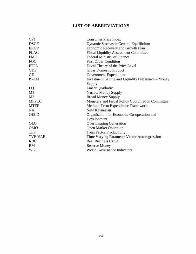
LIST OF ABBREVIATIONS
CPI Consumer Price Index
DSGE Dynamic Stochastic General Equilibrium
ERGP Economic Recovery and Growth Plan
FLAC Fiscal Liquidity Assessment Committee
FMF Federal Ministry of Finance
FOC First Order Condition
FTPL Fiscal Theory of the Price Level
GDP Gross Domestic Product
GE Government Expenditure
IS-LM Investment Saving and Liquidity Preference – Money
Supply
LQ Linear Quadratic
M1 Narrow Money Supply
M2 Broad Money Supply
MFPCC Monetary and Fiscal Policy Coordination Committee
MTEF Medium Term Expenditure Framework
NK New Keynesian
OECD Organisation for Economic Co-operation and
Development
OLG Over Lapping Generation
OMO Open Market Operation
TFP Total Factor Productivity
TVP-VAR Time Varying Parameter-Vector Autoregression
RBC Real Business Cycle
RM Reserve Money
WGI World Governance Indicators

xvii
LIST OF APPENDICES Page
Appendix 1: Prior 198
Appendix 2: MCMC Univariate Diagnostics 200
Appendix 3: Dynare Code for Bayesian Estimation 203
Appendix 4: Dynare Code for Optimal Ramsey and Benevolent Government 206
Appendix 5: Dynare Code for Optimal Ramsey and Rent-seeking Government 208
Appendix 6: Dynare Code for Optimal Discretionary and Benevolent Government 210
Appendix 7: Dynare Code for Optimal Discretionary and Rent-seeking Government 212
Appendix 8: Derivation of the optimal pricing equation for the firm 214
Appendix 9: Prior-Posterior Plot 216

xviii
ABSTRACT
A political economy environment typified by political corruption, poor implementation of
economic policy rules and weak policy coordination, can alter the fiscal behaviour of
government and how it interacts with the monetary policy of the Central Bank. This study
solved and estimated a Small Open Economy New Keynesian Dynamic Stochastic General
Equilibrium model with a modified fiscal bloc. This is done in order to examine fiscal and
monetary policy interactions under alternative assumptions of a rent-seeking government that
follows discretionary policies and where no economic policy coordination exists. Its specific
objectives were to assess the nature of fiscal policy interactions with monetary policy in
Nigeria; examine the transmission effect of the policy interactions on output and inflation, and
to investigate the optimal fiscal and monetary policy mix that guarantees economic stability in
Nigeria. A first-order Taylor approximation method was used to solve the model around its
deterministic steady state. Thereafter the Bayesian method, specifically the Metropolis-
Hastings algorithm was used to estimate the parameters of the model. In order to derive the
optimal combination of fiscal and monetary policy, the Dynare computational routines on
Ramsey policy and Discretionary policy were employed. The results from this study revealed
that both fiscal policy and monetary policy act as strong substitutes. This highlights the
possibility of conflicts between fiscal and monetary decisions. Secondly, the overall impact of
policy interaction negatively affects both inflation and output. This corroborates the lack of
coordination between both policies. Moreover, it implies that stabilisation policies may be
inadequate in guiding the Nigerian economy. Thirdly, the results on the optimal fiscal-
monetary combination point out that politicians and bureaucrats in government should commit
to policy rules. At the same time, they should implement policies that enhance the welfare of
the entire citizens, not just a subset of the citizens. In addition, the study recommends among
others that fiscal and monetary policies should be harmonised. For instance, the Central Bank
of Nigeria and the Federal Ministry of Finance can adopt the same economic model and
assumption in planning and forecasting policy targets.
Keywords: Fiscal and Monetary Policies, Policy Interactions, Optimal Policy, Rent-seeking,
DSGE.

1
CHAPTER ONE
INTRODUCTION
1.1 Background of the Study
Fiscal and monetary policies are the two most significant tools available to policymakers, in
guiding an economy, towards attaining desired macroeconomic objectives which include high
and sustainable economic growth, price stability, employment and viable external balance. The
government employs fiscal tools such as spending and taxes to provide public goods, to
redistribute income and stabilise aggregate demand. The Central Bank also uses interest rate,
exchange rate and money supply to stabilise the price level, output and the financial system.
Both policies are used for the short-term stabilisation of the economy which guarantees
medium to long-term outcomes in growth and welfare (World Bank, 2014). Based on their
importance, governments and central banks, the fiscal and monetary authorities respectively,
are constantly faced with the task of setting the appropriate policy targets that get the economy
closest to its optimal state.
However, there is a lack of consensus on the most appropriate manner that policymakers can
utilize fiscal and monetary policies (Mundell, 1962; Wren-Lewis, 2011). This concern, in
specific terms, whether the instruments of fiscal and monetary policies are independent or
intertwined in their impact on the economy. Debates in the academic and policy-making circle,
between the Keynesian and Monetarist schools of economic thought, implicitly posits fiscal
and monetary policies as separable in nature, since it centred on the importance of each policy,
relative to the other (Hetzel, 2013). This argument is premised on the notion that the
importance and macroeconomic effect of either policy can be isolated from the other (Hallett,
Libich and Stehlik, 2011). But in the literature, inquiry into this debate remains inconclusive
indicating that there is no consensus on the most preferred policy regime, between monetary
2
and fiscal, that an economy should adopt (Mundell, 1962; Ajayi, 1974; Ajisafe and Folorunso,
2002; Musa, Asare and Gulumbe, 2013).
Policy discourse has, therefore, evolved into the proposition that fiscal and monetary policies
are interdependent rather than separate (Niemann and Hagen, 2008). This proposition borders
on the view that ongoing interactions exist between both policies. Policymakers belonging to
this school of thought usually canvass that fiscal and monetary instruments should be combined
in addressing any macroeconomic issue. The central argument, therefore, is to mix or interact
fiscal and monetary policies since externalities are assumed to exist between the two policies,
such that a change in one influences the stance of the other and its overall macroeconomic
effect (Niemann and Hagen, 2008). In other words, the successful outcome or effectiveness of
fiscal (monetary) policy depends on the stance of (monetary) fiscal policy. For instance, rising
and uncontrolled budget deficits can constrain the ability of the central bank to control inflation
rates. This is because rising budget deficit can induce the government to resort to seignorage
revenue from the central bank. The government, in this instance, can pressure the central bank
to print new money in order to finance its fiscal shortfall. Money is consequently injected into
the economy and in turn, the apex bank responds by using restrictive monetary policy to control
the resulting inflation.
The issue of fiscal and monetary policy interactions, therefore, has come to fore, arising from
numerous theoretical and empirical contributions. Tinbergen (1952) argued that fiscal and
monetary policies should be considered as a coherent entity and separately. Similarly, Theil
(1957) opined that policy authorities should combine fiscal and monetary instruments in the
right proportion in order to simultaneously attain desired policy outcomes. In the modern
literature, Sargent and Wallace (1981), Leeper (1991), Sims (1994), Leeper and Leith (2015),
highlighted the need for fiscal and monetary interactions in order to determine price level. They
showed that the effectiveness of policy instruments of the Central Bank- to stabilise and control
inflation- depends to a large extent, on the fiscal stance of the government. Fiscal and monetary
policy interaction is also relevant in its impact on medium to long-term outcomes such as
public debt (Cochrane, 2001; Niemann and Hagen, 2008) and economic welfare (Beningno
and Woodford, 2004; Schmitt-Grohe and Uribe, 2007).
3
Furthermore, economic events like the formation of the European Monetary Union and the
aftermath of the global financial crisis has sparked interest in the issue of fiscal and monetary
policy interaction (Petreveski, 2013; Reserve Bank of India, 2013). The European Monetary
Union (EMU), for instance, is modelled as fielding an economic policy game between several
national fiscal authorities and a single central bank, the European Central Bank. The union's
only apex bank is bound by the Maastricht Treaty to focus on price stability while the various
fiscal authorities are subject to the Pact of Stability and Growth that sets limits on debt and
deficit ratios. Both policymakers within the union, therefore, are expected to act together.
In the same vein, the global financial crisis also underscores the essence of the interrelation
between the government and the Central Bank. In the aftermath of the crisis and the recession
following, some advanced economies opted for expansive fiscal policy. In this regard,
policymakers resorted to applying fiscal instruments in the form of bailouts and stimulus, due
to the ineffectiveness of monetary policy to stimulate the economy at the Zero Lower Bound
rate. The United States, in particular, injected US$125 billion in implementing the Economic
Stimulus Act and US$787 billion under the American Recovery and Reinvestment Act (Kliem,
Kriowoluzky and Sarferaz, 2015). The expansionary nature of fiscal stimuli has posed a
challenge in the manner that inflationary and debt sustainability pressures mounted from the
accompanying rise in deficits and debts. Monetary authorities are therefore concerned with the
looming effect of government expanding stance on their ability to stabilise the price level. This
is because government deficits and debts have the potential to constrain the central banks from
achieving their primary objective of controlling the price level (Sargent and Wallace, 1981;
Leeper, 1991). It is then important to find out how to fix the right monetary targets that
complement such impending bleak fiscal reality (Leeper, 2013).
The concern for fiscal and monetary policy interaction in Nigeria stems from the need for
policy alignment between the Central Bank of Nigeria (CBN) and the Federal Ministry of
Finance (FMF). The absence of coordination between both policy authorities can constrain the
effectiveness of their policies and is a potential source of instability and lower macroeconomic
performance. There is evidence of weak coordination of fiscal and monetary policy in Nigeria,
despite the enactment of institutions such as the Fiscal Liquidity Assessment Committee

4
(FLAC) and the Monetary and Fiscal Policy Coordination Committee (MFPCC) (Englama,
Tarawalie and Ahortor, 2013; Oboh, 2017). The measuring rod of coordination between fiscal
and monetary policy is when both policies have similar stances in the instrument of budget
balances and real interest rate i.e. expansionary fiscal/expansionary monetary and tight
fiscal/tight monetary (Rothenberg, 2004). Available facts, however, show that over the period
1970-2015, fiscal and monetary policies were uncoordinated across 25 years but
complementary in 21 years. This depicts the weak form of policy coordination between both
policies (see section 3.5)
A second argument on the need to study fiscal and monetary policy interaction is to help guide
the design of a consistent set of policies that will consolidate the ongoing Economic Growth
and Recovery Plan of the Federal Government at reviving the Nigeria economy after a bout of
stagflation. Data from the National Bureau of Statistics (2016) reveal that the economy slipped
into a recession after it contracted by -0.36 percent and -2.06 percent in 2016Q1 and 2016Q2.
At the same time, the Inflation rate in Nigeria rose from an average of 12.24 percent over the
period 1996-2016 to 17.6 and 18.10 percent in August and October 2016. The central bank,
therefore, responded by tightening its stance. It raised the Monetary Policy Rate from 11 to 12
percent in March 2016. This was further increased to 14 percent in July 2016, in order to rein
in on the rising inflationary trend. The Federal Ministry of Finance, on the other hand, pursued
an easy fiscal stance. In 2016Q1 and 2016Q2, the budget deficit stood at N548.42 billion and
N1090.96 billion, respectively. Policy analysts deduced that the twin problems of negative
economic growth rate and rising inflation were aggravated by the conflicting and
uncoordinated stances of both fiscal and monetary policy (Central Bank of Nigeria, 2017).
Therefore, it becomes necessary to complement both policies in the right direction in order to
curtail future recessionary episodes and consolidate the gain of the current recovery plan.
The interaction between fiscal policy and monetary policy in Nigeria is examined within a
New Keynesian Dynamic Stochastic General Equilibrium (NK DSGE) framework. This
framework combines standard Keynesian assumptions such as price stickiness, imperfect
competition and the use of stabilisation policies, with the traditions of microeconomic
foundation and general equilibrium conditions. In the tradition of micro-foundation,
5
macroeconomic models are usually built by aggregating the behaviour of rational
microeconomic agents, i.e. households and firms. The NK DSGE model, therefore, considers
the simultaneous economic interaction among households, firms, a Central Bank that sets
monetary policy and a government that fixes fiscal policy, under the assumptions that
optimising agents form rational expectations and the Central Bank and government each
commit to policy rules among others.
Stemming from the preceding paragraphs, this thesis empirically characterises the existing
nature of policy interaction in Nigeria. The thesis also gauges the effect of the policy
interactions on output and inflation in Nigeria. The study, by implication, also obtains the
optimal fiscal and monetary mix that should enhance the outcome of both policies and the
overall macroeconomy.
1.2 Statement of Research Problem
This study investigates fiscal and monetary policy interactions in a small open economy, New
Keynesian Dynamic Stochastic General Equilibrium (NK DSGE) model where certain
theoretical assumptions are altered. Several empirical studies have examined fiscal-monetary
policy interactions within a DSGE model (Muscatelli, Tirelli and Trecroci, 2005; Davig and
Leeper, 2009; Algozhina, 2012; Cekin, 2013; Gilksber, 2016; Chen, 2017). The DSGE
framework provides an appropriate setting to investigate policy interactions. This is because it
assumes ongoing interdependencies among several economic agents that includes households,
firms, central bank and the government. Furthermore, the DSGE-based method is premised on
theoretical assumptions that are relevant for policy analysis. It is, therefore, immuned from the
susceptibility of other estimation techniques to the Lucas’ critique. However, a fallout is that
some assumptions used in the DSGE models are unsuitable in the context of developing
economies (Vangu, 2014). Some of these unsuitable assumptions pertain to the behaviour of
government, that is, the fiscal policy bloc of the model. Several studies examining fiscal-
monetary policy interactions, in this respect, have assumed rather unrealistically that
government is benevolent and at the same time, commits to policy rules.
Empirical evidences such as the Corruption Perception Index (2016), World Governance
Indicators (2016) and the Fiscal Rule Dataset (2017), nonetheless, show that these

6
conventional assumptions do not hold for a developing economy such as Nigeria. This study,
therefore, abstracts from these conventional assumptions. The conventional assumption of the
fiscal sector is then modified in line with political economy literature such that, the government
is posited to be neither benevolent nor does it commit to a policy rule (Persson, 2001; Fragetta
and Kirsanova, 2010; Miller, 2016). The government, however, is assumed to have rent-
seeking tendencies and prefers to use policy discretion in maximising the welfare of a subset
of the society. The modifications to the fiscal bloc can also be used to capture the weak
coordination between fiscal and monetary policies in Nigeria (Englama, Tarawalie and
Ahortor, 2013). It is, therefore, needful to investigate the existing policy interactions when
alternative fiscal realities are explicitly modelled.
This study is, therefore, related to empirical studies that assess fiscal and monetary policy
interactions in Nigeria (Chuku, 2010; Okafor, 2013; Musa et al., 2013). This study nevertheless
differs from them by adopting the DSGE method. However, this study is most related to
Adegboye (2015). His study is one of the few studies that investigate fiscal and monetary
policy interaction in Nigeria, using the New Keynesian DSGE framework. This thesis differs
from Adegboye (2015) because the study considers fiscal and monetary policy interaction in
the form of a fiscal rule in government spending and a Taylor rule, but leaves out the possibility
of policy discretion and rent-seeking which is more related to government’s fiscal behaviour
in Nigeria. Secondly, the work was silent about capturing the poor coordination that exists
between fiscal and monetary policies in Nigeria, since there is empirical evidence of weak
coordination in Nigeria (Englama, Tarawalie and Ahortor, 2013).
This study has consequently identified four research gaps to fill. First, there are few studies on
fiscal and monetary policy interaction in Nigeria. Second, few studies have applied the DSGE
method in Nigeria, even fewer are works that have used the DSGE technique to analyse fiscal
and monetary policy interaction. This thesis contributes to the sparse literature on dynamic
general equilibrium modelling in Nigeria which only a few researchers such as Alege (2008);
Olayeni (2009); Adebiyi and Mordi (2010); Alege (2012) and Adegboye (2015) among others,
have ventured into. Third, this work borrows from the political economy contributions of
Persson (2001) and Miller (2016) to study fiscal and monetary policy interactions in a DSGE
model where existing assumptions about the fiscal authorities are modified to capture the

7
political economy reality of Nigeria. Fourthly, an interaction variable is constructed in order
to explicitly define fiscal-monetary policy interactions.
1.3 Research Questions
Following the need to examine the fiscal and monetary policy interaction under alternative
assumptions of a rent-seeking government that follows discretionary policies and absence of
economic policy coordination, this study seeks to answer the following questions:
i. To what extent does fiscal policy interact with monetary policy in Nigeria?
ii. What is the transmission effect of the policy interaction on output and inflation in Nigeria?
iii. What is the optimal fiscal and monetary policy mix that guarantees output and inflation
stability in Nigeria?
1.4 Research Objectives
The broad objective of this thesis is to examine the interactions between fiscal and monetary
policy under alternative assumptions. The specific objectives are to:
i. assess the extent to which fiscal policy interacts with monetary policy in Nigeria;
ii. examine the transmission effect of the policy interactions on output and inflation in Nigeria;
and
iii. investigate the optimal fiscal and monetary policy mix for output and inflation stability in
Nigeria.
1.5 Research Hypotheses
The study tests the following hypotheses stated in both null and the alternative:
H01: Fiscal policy has no interaction with monetary policy in Nigeria
H11: Fiscal policy has interaction with monetary policy in Nigeria
H02: There is no transmission effect of the policy interaction on output and inflation in Nigeria
H12: There is a transmission effect of the policy interaction on output and inflation in Nigeria
H03: There is no optimal fiscal and monetary policy mix for output and inflation stability in

8
Nigeria
H13: There is an optimal fiscal and monetary policy mix for output and inflation stability in
Nigeria
1.6 Scope of the Study
This thesis runs on two central themes: the impact of fiscal behaviour on monetary decisions
and the optimal mix of fiscal and monetary policy in Nigeria. First, the study displayed some
empirical facts on fiscal-monetary policy interaction in Nigeria using relevant fiscal and
monetary policy targets and instrument variables such as budget deficits, public debt, money
supply, interest rates and inflation rates.
The work then undertakes both positive and normative analysis. In the positive analysis, this
thesis considers whether and how fiscal policy variables such as government spending, budget
deficit, debt influences the Central Bank’s goal of low and stable inflation. In case of the
normative study, the work draws from literature on macroeconomic policy design to conduct
some sensitive policy analysis in order to determine optimal fiscal and monetary policy mix.
The study covers the period from 1961Q1 to 2016Q4. This period is regarded as sufficient in
the sample for analysing fiscal and monetary policy interaction in Nigeria. The study period is
also characterised by several shifts in both policies that are necessary for interaction between
them. These include changes in government that can influence fiscal behaviour and the period
of no independence and operational independence for the Central Bank of Nigeria.
1.7 Significance of the Study
The attempt to examine the extent of interaction between fiscal policy and monetary policy,
and the optimal manner that fiscal and monetary policy should interact, is germane on two
grounds. First, it can be taken as a template to empirically guide the interaction between both
policy institutions in the future, so that policymakers can formulate and plan macroeconomic
targets such as inflation rates, debt levels and growth rates for the Nigerian economy.
Secondly, policymakers can also identify and quantify the transmission of fiscal actions on
monetary policy and the aggregate economy. Thirdly, the work contributes to the relatively
9
unexplored literature on fiscal-monetary policy interactions in Nigeria, especially within the
context of modelling the fiscal behaviour of government using alternative assumptions and the
application of the Dynamic Stochastic General Equilibrium framework.
1.8 Method of Analysis
The study, first, employs a-theoretical methods to explain the long-term trend and derive
business cycle properties of relevant fiscal and monetary policy variables. This is in the chapter
where trend analysis and preliminary stylised facts on policy interactions in Nigeria are
generated.
This study then goes ahead to adopt the dynamic general equilibrium framework based on the
New Keynesian school of thought in order to address the set objectives. The procedure used to
analyse the dynamic stochastic general equilibrium model used includes the following: (1)
write down the model (2) Derive the system of equilibrium conditions of the model (3) solve
for the steady state (4) calibrate the parameters (5) solve the model by log-linear approximation
(6) Estimate the deep parameters of the model using the Bayesian method and finally, (7)
simulate the model with necessary counter-factual policy experiments performed.
1.9 Outline of the Study
This work is divided into six Chapters. Chapter one introduces the subject matter, the research
problem is defined in this chapter, questions of the thesis and strategies to answering these
questions are stated. Chapter two reviews the literature on Fiscal and Monetary Policy
Interactions. In this chapter, conceptual, theoretical, methodological and empirical reviews are
presented; research gaps stemming from the literature are also identified. In chapter three, some
stylized facts on fiscal-monetary policy interactions in Nigeria are illustrated. The study's
theoretical framework and methodology make up Chapter four, while the estimation results are
presented in Chapter five and finally, conclusions, policy implication of findings and
recommendations are made in Chapter six.

10
CHAPTER TWO
LITERATURE REVIEW
This chapter provides a comprehensive outline of developments in the literature on the
interactions between fiscal and monetary policy. The chapter is divided into four major
sections: Conceptual, Theoretical, Methodological and Empirical. In the conceptual review,
definitional issues surrounding Fiscal and Monetary policy interactions are examined. Under
the theoretical review, the main theories underlying the economic policy interactions are
outlined and critiqued. For the methodological review, the essentials techniques of estimation
are mentioned and evaluated. Finally, several empirical findings regarding fiscal-monetary
policy interactions are enumerated in the empirical review.
2.1 Review of Definitional Issues
2.1.1 Fiscal and Monetary Policy Interaction
The idea of interactions between Fiscal and Monetary policy springs from the assumption that
both policies are interrelated. This idea reflects in the writing of Tinbergen (1952) who argued
that economic policy should be considered as a coherent entity that is devoid of any form of
isolation. Fiscal and Monetary policies are, in this regard, interrelated in their impact on each
other’s target. This is premised on the ground that there are externalities or spill-over between
the instruments of both policies such that a change in one influences the stance of the other
(Niemann and Hagen, 2008).
Two channels are involved in explaining the existing externalities or spill-over between both
policies. The first channel runs from the influence of fiscal policy on the instruments and
targets of monetary policy. This channel essentially considers the impact of government
expansive stance in deficit and debt, on nominal variables such as interest rate and price level.
This is because rising budget deficit can induce the government to resort to seignorage revenue
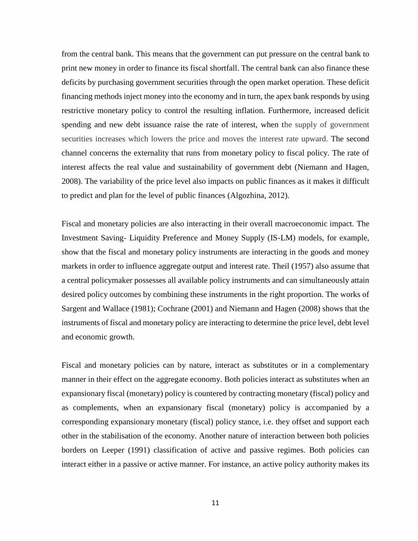
11
from the central bank. This means that the government can put pressure on the central bank to
print new money in order to finance its fiscal shortfall. The central bank can also finance these
deficits by purchasing government securities through the open market operation. These deficit
financing methods inject money into the economy and in turn, the apex bank responds by using
restrictive monetary policy to control the resulting inflation. Furthermore, increased deficit
spending and new debt issuance raise the rate of interest, when the supply of government
securities increases which lowers the price and moves the interest rate upward. The second
channel concerns the externality that runs from monetary policy to fiscal policy. The rate of
interest affects the real value and sustainability of government debt (Niemann and Hagen,
2008). The variability of the price level also impacts on public finances as it makes it difficult
to predict and plan for the level of public finances (Algozhina, 2012).
Fiscal and monetary policies are also interacting in their overall macroeconomic impact. The
Investment Saving- Liquidity Preference and Money Supply (IS-LM) models, for example,
show that the fiscal and monetary policy instruments are interacting in the goods and money
markets in order to influence aggregate output and interest rate. Theil (1957) also assume that
a central policymaker possesses all available policy instruments and can simultaneously attain
desired policy outcomes by combining these instruments in the right proportion. The works of
Sargent and Wallace (1981); Cochrane (2001) and Niemann and Hagen (2008) shows that the
instruments of fiscal and monetary policy are interacting to determine the price level, debt level
and economic growth.
Fiscal and monetary policies can by nature, interact as substitutes or in a complementary
manner in their effect on the aggregate economy. Both policies interact as substitutes when an
expansionary fiscal (monetary) policy is countered by contracting monetary (fiscal) policy and
as complements, when an expansionary fiscal (monetary) policy is accompanied by a
corresponding expansionary monetary (fiscal) policy stance, i.e. they offset and support each
other in the stabilisation of the economy. Another nature of interaction between both policies
borders on Leeper (1991) classification of active and passive regimes. Both policies can
interact either in a passive or active manner. For instance, an active policy authority makes its
12
policy decision without regards to the path of government finance while a passive authority
will respond to changes in the state of fiscal debt (Leeper, 1991).
2.1.2 Working definition of Fiscal and Monetary Policy Interaction
Based on the preceding section, fiscal and monetary policy interaction is defined as the
interplay between both policies with resulting impact on each other’s instruments and on
macroeconomic targets or outcomes.
Some assumptions guiding this working definition include:
1. There are interdependencies between both fiscal and monetary policy;
2. There is a decentralised policy environment such that the two authorities- Central Bank and
Ministry of Finance- are respectively in charge of setting monetary policy and fiscal policy;
and
3. Policy externalities exist between both policies such that changes in one policy induces
changes in the other policy.
2.2 Theoretical Review of Literature
This sub-section shows the underlying macroeconomic theories on the interactions between
the fiscal and monetary policies. A background which summarises the major schools of thought
on economic policy is presented. Thereafter, specific theories on fiscal and monetary policy
interaction are outlined. They include the Monetarist Arithmetic and the Fiscal Theory of the
Price Level.
2.2.1 Macroeconomic Theories up to the New Keynesian School of Thought
The occurrence of the Great Depression of the 1930s in the United States and Europe sparked
the paradigm shift from the classical to the Keynesian school of economic thought (Jahan,
Mahmud and Papageorgiou, 2014). The classical school reflected primarily the works of Adam
Smith and David Ricardo. First, they focused on the underlying factors that spawn and sustain
economic growth. They postulated that an economy is able to reach its potential output or full
employment level in the long run. In the instance of any distortion of the economy from its
13
potential output, the economy can re-adjust on its own in the long run through the price
mechanism. This precludes any form of government policy. The re-adjustment capacity of the
economy demonstrates their liberalist tradition. Essentially, they advocated for minimal
government intervention since the economy is self-correcting. Wages and prices are also
regarded as flexible and determined by the price mechanism.
John Maynard Keynes in his book, The General Theory of Employment, Interest and Money,
differed in his prescription to tackling the Great Depression. Keynes drifted from the
Classicals’ emphasis on aggregate supply to the concept of aggregate demand. The Classicals,
going by the Say’s law, correlated the state of the economy with the level of the aggregate
supply curve. Keynes, in a different manner, posited that the changes in aggregate demand can
distort the actual levels of output from its potential level, creating gaps. Keynes also focused
on the short run, he believed that contrary to the Classicals the economy may never attain full
employment in the long run, because “in the long run we are all dead.” The economy may be
unable to correct itself because prices are sticky in the short run. Keynes, therefore, advocated
for the intervention of the government, specifically the use of fiscal and of monetary policy,
which are termed stabilisation policies, to direct the economy to its level of potential output.
The monetarists led by Milton Friedman link in a direct proportionate manner, changes in the
money supply to changes in the level of output. They opine that only money matters in an
economy (Jahan and Papageorgiou, 2014). They uphold the liberalist view of the Classicals
and likewise argue for minimal intervention of government in the economy. In this respect,
they avoid the use of Keynesian stabilisation policy. Fiscal policy is neutral in its impact due
to its crowding-out effect, while the lags associated with monetary policy can be long and
destabilising. They advocate the implementation of a monetary rule in money supply such that
the central bank increases the money supply at a fixed annual rate.
The New Classicals build on the ideas of the Classicals. They focus on the supply side of the
economy, flexible prices and the ability of the economy to correct itself. The New Classicals
propose the use of sophisticated mathematical economic models with rational agents who
desire to maximise their preferences (Hoover, 2008). This school also centres its analysis on
the rational expectations hypothesis, which assumes that individuals form expectations about

14
the future based on the information available to them, and that they act on those expectations.
The New Keynesians adopts the conventional argument of sticky prices and the effectiveness
of stabilisation policy in returning an economy to the level of the potential output and also
incorporates the aggregate supply bloc into their model. They also adopt a mathematical model
of the aggregate economy built upon microeconomic foundations (Mankiw, 2008).
2.2.2 Models of Fiscal and Monetary Policy Interactions
The major theories explaining fiscal-monetary policy interaction are presented and reviewed
by highlighting their similarities and differences, strengths and weaknesses as well as existing
gaps. These theories underlying fiscal-monetary policy interaction are the IS-LM model, the
Monetarist Arithmetic (Sargent and Wallace, 1981; McCallum, 1984) and the Fiscal Theory
of Price Level (Leeper, 1991; Sims (1994, 1999); Woodford (1995, 1996, 2001). These
theories, especially the Monetarist Arithmetic and Fiscal Theory of Price Level, are set within
the mathematical model and rational expectation framework of the New Classical and New
Keynesian schools of economic thought.
a. The Investment Saving and Liquidity Preference – Money Supply (IS-LM) model
The IS-LM model is used for policy analysis to depict the manner in which fiscal and monetary
policies interact to determine the level of aggregate output and interest rate. The IS curve
represents equilibrium in the goods market which shows that aggregate spending is defined as
the summation of private household consumption, investment spending by firms and purchases
by the government. The LM curve on the other hand, represents equilibrium in the
money/financial market such that real money supply equates money demand.
The two curves intersect to uniquely determine the aggregate output (Y) and interest rate (r).
The interaction between fiscal and monetary policy in this model occurs whenever there is a
change in one policy such that the other adjust its path to this change. For instance, when there
is a change in fiscal policy such that the government increases the level of spending or lowers
taxes, this affects the goods market and shifts the IS curve to the right. Mankiw (2016) notes
that the central bank can respond to this change in three ways. These include holding constant
the level of money supply, the interest rate and the level of output. In the case that the central
bank responds by holding the level of money supply constant, the level of output in the goods

15
market increases as well as spilling over to the money market where the interest rate equally
rises. When the central bank reacts to a change in the policy of government by keeping the rate
of interest fixed, then it shifts the LM curve to the right and the level of money supply rises.
This scenario is in fact further modelled in a formal manner. Finally, in the face of reacting to
fiscal policy by holding the level of aggregate output unvaried, the central bank will have to
shift the LM curve to the left which indicates that the volume of money in circulation reduces.
b. Monetarist Arithmetic
The seminal contribution to the concept of the Monetarist Arithmetic was by Sargent and
Wallace (1981). It highlights the idea that central bankers are required to regard the
government’s fiscal policy, while making policy decisions. This is because government actions
can render ineffective the ability of monetary authority to determine and stabilise price level
in the economy. Sargent and Wallace (1981) define fiscal-monetary policy interaction as a
Stackelberg game between the Central Bank and Treasury. They demonstrate that in a fiscally
dominant regime, the central bank may find it difficult to control inflation since it may be
unable to decide the path of money stock given the exogenously determined path of
government’s budget deficit. In arriving at this conclusion, they draw on a monetarist model
embedded in an Over-Lapping Generation framework. In this model, they centrally assume
that the path for government deficit is exogenously determined i.e. the government is assumed
to set the deficits, while the central bank controls the level of money supply and can raise
revenue from money creation. In the model, fiscal and monetary policies are interacting within
a consolidated government budget constraint. This constraint is an identity that links both
policies. It shows that the government finances its budget deficit by issuing one-period bonds
and by money creation.
The path of fiscal policy is, therefore, assumed to exogenously evolve under this form of policy
game; while the central bank passively adjusts to the path of this government policy. Under
this circumstance, for every deficit the government fixes, the central bank is forced to finance
it through money creation, if it cannot be financed by the sale of bonds. The central bank is
also constrained to finance government deficit if the economy reaches a fiscal limit where the
government can no longer issue new bonds since it has accumulated a large amount of debt
which it is likely to default on. The creation of money by the central bank either by printing

16
money or buying government securities injects money into the economy, which leads to a surge
in volume of money supplied and by the monetarist quantity theory implies increases in the
price level and then inflation. The solution to the constraint imposed on the central bank is an
independent and conservative authority that can discipline the government by refusing to
finance its deficit.
However, there have been reactions to the position of Sargent and Wallace (1981) as stated
earlier in the previous paragraphs. For instance, Weil (1987) re-examines their conclusion that
primary budget deficits have to be monetized i.e. central banks are restricted from selecting
desired range of money supply in the face of exogenously determined budget deficits of the
fiscal authorities. Weil (1987) adopts a simple monetary model nested within a fusion of the
Over-Lapping Generation and Infinite-Horizon frameworks. The study assumes a monetary
economy with intergenerational dynamics where new and infinitely-lived individuals
continuously enter the economy. The results reveal contrasting conclusions such that when
intergenerational effects are considered, there are larger chances that central banks can
determine the paths of monetary policy for every given fiscal policy. By implication, the
findings of Weil (1987) differs from Sargent and Wallace (1981) on grounds that the study
departs from the standard OLG models and assumes real interest rates that vary. In the same
vein, Darby (1984) counteracts the Sargent and Wallace (1981) assertion. The author shows
that this assertion may not hold under certain conditions. The author overturns Sargent-Wallace
assumption that real interest rates are higher than growth rates, and also modifies their
definition of real interest rate using the after-tax values; but retains Sargent-Wallace
proposition that real interest and growth rates are constant. In a model where real interest rates
are lower than growth rates, Darby (1984) shows that the Sargent-Wallace may not hold.
The conclusions of Weil (1987), Darby (1984) show that the Sargent-Wallace hypothesis may
hold or not depending on the underlying assumptions held or relaxed. McCallum (1984), Miller
and Sargent (1984) prove this. McCallum (1984) examines the monetarist notion that
government budget deficit can be non-inflationary on condition that it is funded by bond sales
rather than from currency. Using a discrete time, deterministic model, the study is able to
illustrate that the validity of this hypothesis depends on whether budget deficits are defined as

17
including interest payments or not. Specifically, the monetarist hypothesis does not hold when
deficits are defined as excluding interest payments. Also, Miller and Sargent (1984) relax the
Sargent-Wallace assumption of an exogenously fixed interest rate. According to the authors,
the real interest rate is partly derived as a function of the ratio of interest-bearing government
bonds to base money. By this, the study uses ad-hoc aggregate demand and supply equations
to show that merely comparing real interest and growth rates as conducted in Darby (1984) is
insufficient to predict the Sargent-Wallace hypothesis.
c. Fiscal Theory of the Price Level
Even though Weil (1987), Darby (1984), McCallum (1984) contradict Sargent-Wallace
hypothesis because they modify some of its assumptions, Buiter (1999) supports this
hypothesis. Apart from the generalization of Sargent-Wallace hypothesis when certain of its
assumptions are relaxed or modified, a second source of contradiction to this proposition is
from Leeper (1991), Sims (1994), Cochrane (2001), Woodford (1995, 2001). This set of
articles make up the literature on the Fiscal Theory of Price Level (FTPL)
Its proponents argue that fiscal policy is the foremost determinant of price level. Unlike the
monetarists who propose that government budgets indirectly affect the price level through the
seignorage- money stock channel. Woodford (1995, 1996, 2001) and others posit that
government budget can have a direct impact on price level void of any monetary channel. This
indicates that fiscal policy takes on an active role while monetary policy only plays a passive
role in controlling the price level.
One of the key contributions to the literature on the fiscal theory of the price level is from
Leeper (1991). The study shows the joint pairing of fiscal and monetary policy paths which
uniquely determines equilibrium price level. In a specific manner, the study models the
interaction between fiscal and monetary policy as an active and passive game. An active policy
is defined as policy that fixes its path independently from variation to the budgetary condition
or debt shocks while a passive policy responds to budgetary shocks and is constrained by the
actions of the authority with the active policy. A unique determination of the price level,
therefore, requires the pairing of an active policy with a passive policy. For instance, an active

18
monetary policy with a passive fiscal stance and an active fiscal policy coupled with a passive
monetary policy leads to uniquely determined prices. The combination of two passive policies
leads to indeterminacy of the price level, while the pairing of two active policies produces an
explosive path. The fiscal policy in the proposition of the fiscalists, therefore, takes on an active
path while monetary policy is passive in order to uniquely determine the price level.
It suffices to note at this point that there are several issues of contest between proponents of
the Monetarist Arithmetic and the Fiscal theory of the price level. Although, the monetarist
literature comprising the thoughts of Sargent-Wallace assume that there is a budget constraint
on government which is an identity that must be satisfied for all paths of prices, the proponents
of FTPL assumes otherwise. They opine that government budget constraint is fulfilled only for
equilibrium price paths. In dealing with fiscal dominant regimes, the monetarist doctrine
suggests that central banks should become independent and follow a Taylor’s rule in
determining the course of monetary policy. However, Woodford (1995, 1996, 2001) argue that
such recommendation is insufficient in quelling unstable price levels, since government budget
surpluses have direct effects on price levels even in the face of a conservative and independent
central bank. This is because the price level adjusts to maintain inter-temporal government
budget balance. As a result, Woodford (1995, 1996, 2001) advocates fiscal policy as the main
determinant of price levels. Furthermore, he suggests that the pairing of a Taylor rule for
monetary policy with government budget deficits rule for fiscal policy is panacea to achieve
low and stable inflation rates. On similar grounds, Leeper (1991); Leeper and Leith (2015) put
forward that the joint movements of monetary and fiscal policies determine the price level.
Leeper (1991) specifically recommends that monetary and fiscal policies are paired such that
an active policy stance is accompanied by a passive one to realise a low and stable price level.
A second line of contest between FTPL and the monetarist doctrine centres on the existence of
Ricardian or Non-Ricardian fiscal policy. Woodford (1995, 1996, 2001) assumes the existence
of non-Ricardian fiscal policies. Under this setting, Ricardian equivalence as posited under
conventional macroeconomic studies is violated and fiscal policy can have non-neutral effects
on aggregate demand. Specifically, the inter-temporal government budget constraint is
satisfied for some, but not all, price paths. This negates the monetarist doctrine that only

19
Ricardian fiscal policies exist. In addition, a third line of division between both theories rest
on the instrument of monetary policy. While the monetarist considers money stock to be the
instrument of monetary policy, the FTPL of Woodford (1995,1996, 2001) backs the use of
nominal interest rate, since they assume a cashless economy experiencing financial innovations
and have no government-backed money. Like Woodford, Sims (1994) proposes that in a
rational expectation framework, fiscal policy plays a major role in price level determinacy. In
the same vein, Sims (1994) advocates that interest rate rather than money stock leads to unique
price paths. But, Sims’ point of departure is his assumption of an economy with frictionless
market as Woodford assumes the presence of nominal rigidity.
Although authors of the FTPL critique the monetarist notion, their contributions have also been
scrutinized. For instance, Christiano and Fitzgerald (2000) support their assertion, so does
Cochrane (2001). Both show the plausibility of FTPL models. However, some writers such as
Buiter (1999, 2002), Niepelt (2004), Kocherkalota and Phelan (1999) are pessimistic of the
FTPL strand of literature. Niepelt (2004) demonstrates that the FTPL model fails to produce
unique and equilibrium price paths when analysed in a different model, specifically in a cash-
in-advance (CIA) constraint model with postulations of a positive interest rates and a money
supply target. Furthermore, Buiter (1999, 2002) shows that the FTPL has a fundamental
economic flaw. The author argues that the FTPL model confuses government budget
constraints with equilibrium conditions. Just as Niepelt (2004), Buiter (1999, 2002) also argues
that FTPL postulations hold only in models where monetary policy is specified as interest rates.
Equilibrium price level is over-determined in models where this assumption is altered.
In summary, both theories similarly adopt the central ideology that the fiscal policy is
important for price level determinacy, and are mainly concerned with short-term stabilisation
issues. However, Canzoneri, Cumby and Diba (2001) surmise the major difference between
the FTPL and monetarist arithmetic. While the monetarist arithmetic viewed fiscal-monetary
policy interaction as a non-cooperative game between the government and its central bank and
believed that coordination of fiscal-monetary policy produced Pareto improving outcomes. By
contrast, the FTPL coined the problem of fiscal-monetary policy interaction as one that
concerns design of the right combination of policies to provide stable economic outcomes.
Other dividing themes between both theories centre on four issues: their assumptions of the
20
inter-temporal government budget constraint, whether fiscal policy follows a Ricardian or non-
Ricardian process, using either the money stock or interest rate as a tool of monetary policy
and whether government debt is nominal or real. In addition to the four theoretical issues that
have been spotted, another major theoretical gap is the emphasis on stabilisation, leaving out
long term issues such as debt or structural reforms. However, Cochrane (2001), Leeper and
Leith (2015) comprise the few articles which consider long-term debt issues. Other theoretical
gaps span across whether a consolidated government budget constraint should be prescribed
in the face of a decentralised policy environment and whether the assumption of an exogenous
fiscal policy holds.
In relation with the theoretical gaps identified, this study considers the strengths and defects of
both theories. The thesis outlines theoretical assumptions that synchronises the best of both
theories and that holds in the Nigerian context.
2.3 Methodological Review
The existing methods that have been used by researchers to analyse the interactions between
fiscal and monetary policy are categorized as a-theoretical, game theoretical and dynamic
general equilibrium framework. The a-theoretical method involves pure statistical analysis of
economic phenomena, while the game theoretical and dynamic general equilibrium methods
are essentially computational-based techniques. Generally, computational techniques use
numerical methods to solve economic models that assume that economic agents such as
households, firms and policymakers, are interacting according to rules. One is usually
interested in deriving equilibrium outcomes and the relevant rules underlying such interactions.
In the two methods, it is assumed there are economic agents who are concerned with optimising
their objective functions in the face of economic constraints. This sub-section presents a review
of some studies that have employed these three methods.
2.3.1 A-theoretic Statistical Methods
The a-theoretical statistical approach has been used in a number of studies to capture fiscal-
monetary policy interactions. A-theoretic methods are concerned with the statistical
measurement of economic phenomena without relying on economic theory. In this group of
21
studies, statistical measures serve as the basis for deciding the existing form of interaction
between fiscal and monetary policy (Alege, 2008).
The studies by Nyamongo, Sichei and Mutai (2008), Rothenberg (2004), Montoro, Takats and
Yetman (2012) began their examination of fiscal and monetary policy interaction by
characterising the cyclical properties of each policy i.e. whether they are procyclical or
countercyclical and each policy stance i.e. whether they are tight or loose. In this regard, the
most widely adopted measure of fiscal policy in these studies is the structural or cyclically-
adjusted budget balance. The cyclically-adjusted budget balance is obtained by removing the
business cyclical component of the budget balance from its nominal component. On the other
hand, monetary policy is captured by the real interest rate or the policy rate of the Central Bank.
Once each policy has been appropriately measured, they are thereafter characterised. For
instance, Montoro, Takats and Yetman (2012) examined the cyclical properties of both
policies. They estimated the correlation between the cyclical component of Real Gross
Domestic Product (GDP) and the real interest rate on one hand, and the correlation between
the cyclical component of Real Gross Domestic Product and budget balance as a percent of
GDP on the other hand. Large and positive values of the correlation parameter imply a
countercyclical fiscal/monetary policy while a negative value means that fiscal/monetary
policy is procyclical. Rothenberg (2004) also investigated the nature of the policy stance. He
interpreted positive values of the cyclically-adjusted budget balance as an expansionary/loose
fiscal stance while negative values mean a contractionary/tight fiscal stance. Conversely,
Carlson (1982) interpreted negative values of real interest rates as tight monetary policy while
its positive value means that monetary policy is loose.
After characterising the cyclical properties and stance of both policies, the nature of interaction
existing between both policies can then be investigated. Nyamongo, Sichei and Mutai (2008)
for example, investigated policy interaction in Kenya with respect to the extent of coordination
between both policies. In the study, both policies are interpreted as being coordinated when
they simultaneously take on a tight/tight stance or a loose/loose stance. In a related manner,
Rothenberg (2004) used the pairwise correlation statistic to examine the nature of interaction

22
between the policy rate of Federal Reserve and the adjusted budget balance of the United States
government. The author found a statistically insignificant and negative correlation between
both fiscal and monetary policy, which is interpreted as evidence of no coordination.
The a-theoretical statistical approach also includes estimation techniques that depend primarily
on statistics without relying on economic theories. Relevant a-theoretic estimation techniques
that have been applied in the context of research on fiscal and monetary policy interactions
include Granger Causality, Cointegration and Vector Auto regression techniques. For example,
Janků and Kappel (2014) used a multivariate regression analysis to examine fiscal and
monetary policy interaction in countries of the Visegrad Group: the Czech Republic, Slovakia,
Poland and Hungary over the period 2000Q1- 2012Q4. The authors estimated fiscal and
monetary reaction functions for each country using twelve separate equations. The authors
conducted unit root tests on variables used, in order to ensure stationarity and to avoid spurious
regression. The result of the study showed that monetary policy has stabilising effect, such that
inflation and output gap significantly respond to it both in a negative and positive manner. The
fiscal policy too has stabilising effects on the economy to some extent. Furthermore, the study
found that fiscal policy significantly adjusts to monetary policy in three out of the four sample
countries: Czech Republic, Slovakia and Poland. This means that there is monetary dominance
in these countries. However, the study left out diagnostic testing of parameter values for
violation of assumptions of ordinary least square estimates.
Reade (2011) used a cointegrated VAR method to assess monetary and fiscal interactions in
the United States over the period 1982Q1- 2010Q2. The author found that, monetary policy
has a passive stance while fiscal policy has an active stance. Both policies are revealed to
complement each other. Muscatelli, Tirelli and Trecroci (2002) estimated VAR and Bayesian
VAR models for 5 OECD countries: Germany, France, Italy, the United Kingdom, and the
United States, using quarterly series comprising the output gap, the inflation rate, a measure of
fiscal stance and the interest rate, in order to examine fiscal and monetary policy interactions
and their effects on macroeconomic targets. The authors estimated for fixed parameters in the
conventional VAR technique, in order to assess whether fiscal and monetary policy interact as
substitutes or complements. The study, then, estimated for time-varying policy parameters
23
using the Bayesian VAR model, so as to capture any regime shift in fiscal and monetary policy
interactions over time. The study found asymmetry in the interaction between fiscal and
monetary policies in some countries. The study also provided evidence that the nature of
interdependence between fiscal and monetary policy has shifted over time.
Franta, Libich and Stehlík (2012) also used the Time Varying Parameter VAR to analyse the
interactions between fiscal and monetary policies, in terms of how monetary authorities
respond to government spending shocks, comparing countries with inflation targeting and non-
inflation targeting regimes. The authors estimated the Bayesian VAR models comprising of
five variables in output, private consumption, the short-term interest rate, government spending
(consumption and investment), and government debt over the period 1980Q1–2008Q2 for the
economies of Australia, Canada, Japan, Switzerland, the UK, and the U.S. The authors then
obtained impulse response functions of the variables assuming a spending shock. The result of
the study showed that central banks in inflation-targeting regimes can withstand not
accommodating government’s spending shocks. Gerba and Hauzenberger (2014) also used the
TVP-VAR to examine fiscal and monetary policy interaction in the United States. The fallout,
however, of the a-theoretic approach is their susceptibility to the Lucas’ critique.
2.3.2 Game Theoretic Models
Blinder (1982), Alesina and Tabellini (1987) are examples of early application of game theory
models to issues on economic policy interactions. In these studies, fiscal and monetary policy
can be modelled as relating in three ways: as a single, unified policy maker- who can set both
fiscal and monetary targets; as independent institutions with no coordination; and in a leader-
follower interaction (Blinder, 1982). Moreover, these studies use the linear-quadratic
constrained optimisation technique, to analyse a policymaker who maximises a (quadratic)
policy preference or minimises loss functions in policy instruments subject to economic
constraints. Two important results are usually obtained: first, the policy reaction functions
which is a rule that depicts how one agent responds to the action of others and then, the
equilibrium policy solutions. The equilibrium solution is usually an optimal rule in specified
fiscal and monetary policy variables like interest rates, money supply, government spending
and deficits. Once the policy reaction functions and equilibrium solutions are computed, some

24
studies proceed further to estimate the parameters in these functions and simulate using a
computational iterative method that converges.
Alesina and Tabellini (1987) examined fiscal and monetary policy interaction in a static-
deterministic policy game that consists of three economic agents- the central bank, fiscal
authority and wage setters. Using the quadratic programming and constrained optimization,
the authors minimise the quadratic loss functions of both fiscal and monetary authorities as
deviations of inflation and outputs from their targets. Then the authors computed the policy
reaction functions of the fiscal and monetary authorities in government expenditure and money
supply, under assumptions of both discretionary and rule-based policy regimes. In a related
manner, Nordhaus (1994) also used a linear-quadratic programming to solve a constrained
optimisation problem of a static game model. In this model, fiscal and monetary authorities
seek to maximise different preferences in inflation, unemployment and potential output subject
to constraints on the economy. From this, the study derived first-order conditions and computes
both fiscal and monetary policy reaction function in budget deficit and real interest rate.
Bartolomeo and Gioacchino (2004) studied fiscal-monetary policy interaction in a dynamic
two-stage game and within a long run (public debt) context. This contrasts with the static games
of Alesina and Tabellini (1987); Nordhaus (1994). In the first stage, the authors derived
equilibrium conditions, preferably the correlated equilibria. Then output from the first stage is
imputed in the differential game of the second stage. In this stage, central bank and the
government minimise their inter-temporal loss functions subject to government budget
constraints. The introduction of government budget constraints differs from the approach of
Alesina and Tabellini (1987); Nordhaus (1994) who only specify aggregate supply functions.
The authors compute policy reaction functions in money supply and fiscal deficits.
Apart from the policy reaction functions computed from solving game theoretical model, the
solution concept of these games is a second trend worth mentioning. The essential solution
concepts are the cooperative and non-cooperative (Nash and Stackelberg). Games in the non-
cooperative realm assume that the treasury and central bank optimise separate loss or
preference functions. However, for the cooperative solution, the game is modelled as both

25
fiscal and monetary policy makers optimising on a consolidated loss or preference function
subject to economic constraints. This idea of a consolidated objective function reflects the
existence of fiscal and monetary policy coordination than the non-cooperative solutions.
Petit (1989) computed cooperative and non-cooperative (Nash and Stackelberg) equilibria of
a differential game between treasury and the central bank. Here each policy maker is modelled
as choosing optimal policy strategies by minimising a quadratic loss function subject to
economic constraints defined as an econometric function comprising of a system of 20
differential equations. Just like Petit (1989), Hallett and Weymark (2007) also derive
cooperative and non-cooperative solutions. The study computes optimal fiscal and monetary
policy rules in expenditure and money supply using the Nash and Stackelberg solutions to a
two-stage dynamic game between the government and the central bank. In the first stage, the
requisite institution is designed. In the second stage, both authorities set their policy
instruments, expenditure and money supply respectively, given the already designed institution
in stage one. Specifically, both authorities minimise their respective loss functions. Also,
Saulo, Rego and Divino (2013) solve for optimal fiscal and monetary policies paths under three
coordination regimes: Nash, Stackelberg and Cooperative. In the dynamic game, both policy
authorities seek to minimise their respective quadratic loss function subject to micro-founded
economic constraints in IS function, Aggregate supply and the Government Budget constraint.
Thereafter, the authors employ numerical simulation to calculate the loss associated with each
coordination regime.
Another aspect to the game-theoretic methods is game models with micro foundations. Micro-
founded objective functions and economic constraints is a relatively recent trend in the
application of game theoretic models to issues of fiscal-monetary policy interaction. It involves
deriving objective functions and constraint equations from a general equilibrium model
comprising of preferences and technologies of a representative household and firm, alongside
the budget constraint of government. It is noteworthy to emphasise micro-founded game
models, since this underlying micro-structure relates to the method adopted in this study.

26
Adam and Billi (2008) solved a micro founded model from a New Keynesian framework. In
the same vein, Dixit and Lambertini (2003b) build a social loss function micro-founded from
a New Keynesian framework. Here, the two players of the dynamic stochastic game, fiscal and
monetary policymakers are expected to minimise this social loss function in deviation of output
and inflation from target subject to rational expectation constraint. Thereafter the authors
derive separate reaction functions for the two authorities and compute Nash and stackelberg
equilibria under both discretionary and commitment regimes. Then, the authors conduct a
numerical simulation of their model. In the same manner, Hallett, Libich and Stehlik (2011)
consider a policy game between fiscal and monetary authority over the medium term. Here
both policymakers seek to maximise a quadratic policy preference function in inflation and
output, subject to supply-side constraints. The preference functions are micro-founded. From
the constrained optimisation, the study derives reaction function for both the fiscal and
monetary sides in inflation and budget deficits, respectively. In addition, the authors solve for
optimal (Nash) policy in both.
From the review above, three observable methodological trends in game theory are policy
reaction functions, the type of solution concepts computed such as Cooperative, Nash,
Stackelberg, Correlated, Markov-Perfect, etc; and whether the game was micro-derived or not.
However, one methodological issue stands out. This borders on the most realistic approach
used to model the strategic interaction between the fiscal authority and central bank. Are they
involved in a cooperative game with a consolidated objective function or government budget
constraint? or in a non-cooperative game, possessing differing objective functions? Or in a
Markov switch between both cooperative and non-cooperative regimes. Probably, the
institutional setting inherent in the macroeconomic policymaking arena will provide the hint
to aid in realistic modelling of this policy game.
2.3.3 Dynamic General Equilibrium Methods
These dynamic general equilibrium methods are couched within the dynamic general
equilibrium framework. The framework describes that macroeconomic behaviour hinges on
the interaction among microeconomic units. The assumptions of the dynamic general
equilibrium method comprise economic agents such as households, firms, governments and

27
central banks are rational. These agents are assumed to form rational expectations of the future.
The households and firms seek to maximise their preferences and technology subject to
constraints, while governments and central banks interact by specifying policy rules. These
agents live and make their economic decisions in a finite or infinite time horizon, and over a
discrete or continuous space. Dynamic general equilibrium models fall into two major schools:
The Classical Real Business Cycle and New Keynesian Dynamic Stochastic General
Equilibrium models. In this section, the application of both models in studying economic
policy interactions is outlined.
a. Real Business Cycle Models
Real Business Cycle (RBC) models, which is a dynamic general equilibrium apparatus, stems
from the contributions of Kydland and Prescott (1982); Long and Plosser (1983) and others.
The model underlies a business cycle theory which emphasises real shocks, particularly,
unanticipated changes in total factor productivity i.e. technology as the source of economic
fluctuations. Other forms of real shocks such as government purchases, preferences and
expectations are also plausible. The RBC model is also an essential methodological
masterpiece. RBC models, in this respect, are built on the micro foundation of Walrasian
general equilibrium, the basic neoclassical growth models of Solow (1956), Cass (1965),
Koopman (1965), the Ramsey (1928) inter-temporal model and the stochastic growth model
of Mirman and Brock (1972). These models, therefore, assume a representative agent
framework comprising of rational and identical households and firms that have explicit
objective functions which they want to maximise subject to budget and technology constraints.
There is also a perfect frictionless market for labour and capital; and prices adjust
instantaneously. In addition, there is little role for government regulation since markets are
assumed to always clear, furthermore, the model assumes the classical dichotomy where
money is regarded as neutral.
Christiano, Eichenbaum and Evans (2005), Romer (2006) critique that RBC models are unable
to prove the neutrality of money, the dominance of technological shocks in explaining the
cyclical trends in actual economies like the United States and that prices are taken to be
flexible. Furthermore, RBC models assume in a rather unrealistic manner that there are no

28
forms of government regulation. An implication of these assumptions is that RBC models leave
out money and monetary policy and in general, it is traditionally silent on the application of
economic policies. Despite this, Rebelo (2005) notes that RBC models have been useful for
policy analysis as it has been a workhorse for the study of optimal fiscal and monetary policy.
Its usefulness in this regard, may be linked to some extensions to the RBC framework. RBC
models, in some ad-hoc cases, have been modified to include money, government spending,
imperfect competition, among others (Rebelo, 2005).
b. Dynamic Stochastic General Equilibrium (DSGE) Models
DSGE Models are built on the micro-foundation and dynamic general equilibrium framework
just as the RBC model. Their point of departure from RBC models is to abstract away from the
Classical assumptions of frictionless markets, flexible prices and neutrality of money. The
DSGE models stems from the contributions of Smets and Wouters (2003); Gali (2003);
Christiano, Eichenbaum and Evans (2005); Smets and Wouters (2007). In this variant of DGE
models, it is assumed that business cycle is driven by both real and nominal shocks, non-trivial
effect of monetary policy, monopolistic competition, nominal rigidity etc. In the standard
model, there are three agents: the household, firms and Central Banks. The household
purchases goods, holds money and bonds, supplies labour to the firms and maximises its
expected present value of utility. There are two types of firms: intermediate and final goods
firms. The firms produce differentiated products in monopolistic competition. The central bank
sets the nominal interest rate in Taylor-type rules.
The DSGE models have been used for economic policy analysis than its RBC counterpart,
since it recognises a role for stabilising (fiscal and monetary) policies. It can also account for
the effect of both real and nominal shocks on the economy. This study will adopt the DSGE
framework based on the New Keynesian school of economic thought. Therefore, an extensive
discussion of the NK DSGE framework is presented, with a focus on how NK DSGE models
are solved and estimated. This is done in the context of works that have applied the NK DSGE
to fiscal and monetary policy interactions.
29
c. Solving DSGE models
DSGE models often lack an exact and closed form solution that can be cumbersome and messy
with paper and pencil. Their solutions are derived by numerical methods in order to find an
approximated path. In this subsection, some solution methods to solving DSGE models are
presented. The discussion is due primarily to Flotho (2009); Fernandez-Villaverde, Rubio-
Ramirez and Schorfheide (2016). The solution methods are generally classified into the
perturbation and projection Methods. The perturbation solutions are local approximations that
usually involve a Taylor series approximation of equilibrium equations around their non-
stochastic steady state. Fernandez-Villaverde et al., (2016) argue that perturbation methods are
most suitable for solving a medium-scale NK model since it is sufficiently well-behaved.
Linear Quadratic method, linear approximation and second (or higher) order approximation
are some perturbation methods. Projections methods on the other hand, have global solutions.
i. Linear-Quadratic Technique
The Linear Quadratic method is a traditional solution to DSGE models, which begins with
transforming the DSGE model into a linear-quadratic (LQ) problem such that a quadratic
objective function is optimised subject to constraints that are a linear function of the state
variable. This approach was used first by Kydland and Prescott (1982) who used it in solving
a Real Business Cycle model. However, Judd (1996, 1998) as cited in Pierse (2006) pointed
out that the method is invalid in a non-linear model which is typical of the DSGE framework.
The correct approach is therefore to compute a second order approximation to the Lagrangian
function.
Beningno and Woodford (2004) employed this technique to obtain optimal fiscal and monetary
policy paths that determines inflation and output. The authors built a New Keynesian DSGE
model comprising of household that maximises utility subject to budget constraint, firms that
produce differentiated goods and a pricing equation that specifies how price level evolve. The
authors restate the DSGE model in a linear-quadratic form by computing log-quadratic
approximation of the household objective function around its steady state. The study also
derives second-order (log) approximation of constraint equations in Philips curve and the
Government Budget constraint, in order to eliminate any linear term appearing in the quadratic
30
objective function. Beningno and Woodford (2004) do so to arrive at a purely quadratic
objective function. The next step is to minimise the quadratic loss function, resulting from the
previous step, subject to log-linearised constraint equations. The Lagrange method is used, and
a system of first order conditions is derived and solved in terms of inflation, output, tax and
debt.
Leeper and Zhou (2013) also used the linear-quadratic technique, to solve a New Keynesian
DSGE model for optimal fiscal and monetary policy. In a New Keynesian DSGE model, the
authors assume a household sector that maximises objective function subject to budget
constraint, a firm in monopolistic competition that produces differentiated goods using
technology and sets the price. There is also a government sector with an inter-temporal budget
constraint and an equilibrium condition in aggregate resource constraint. Nonlinear constraint
conditions in Philips curve, consumer Euler equation and government budget constraint are
derived from the model. The objective function of the household and constraint equations is
then approximated to second-order to compute a purely quadratic loss function. Thereafter the
loss function is minimised subject to log-linearised constraint equations in order to compute
optimal fiscal and monetary policy in tax and nominal interest rate.
ii. First-Order Approximation
Another traditional solution is the linear approximation method, also known as the first order
approximation, to solving the DSGE model. It involves a Taylor series approximation of the
system of first order conditions of the DSGE model around their steady state. The DSGE model
usually has a non-linear system of equilibrium conditions whose solution may be too difficult
to obtain until the system is linearised using the Taylor series approximation. The method is a
local approximant whose procedures are valid in the neighbourhood of the non-stochastic
steady state. Linearisation can be conducted in log or levels. The first-order linear
approximation is adequate when there are small shocks driving the business cycle and an
interior stationary solution exists (Schmitt-Grohe and Uribe, 2004). In general, it is adequate
for several economic analyses since it leads to a state-space representation of the model, which
is suitable for empirical estimation and forecasting. There is, however, evidence that higher-

31
order approximation leads to better results, in particular for cases of economic welfare and risk
analysis (Flotho, 2009; Fernandez-Villaverde et al., 2016)
Leeper (1991) solved a NK DSGE model to find the fiscal and monetary policy paths that
uniquely determines inflation and government real debt, using the first-order Taylor method.
This method approximates equilibrium equations around the steady state. The model of the
study consists of a representative household that maximises a money-in-utility function with
respect to its budget constraint, government sector with its budget constraint, and stochastic
linear fiscal and monetary policy rules in interest rate and taxes. Leeper (1991) initially solved
the model for Euler equations and equilibrium conditions using the recursive method. The next
procedure is to linearise the equilibrium equations to derive a system of equations in the
endogenous variables. The system of equations is solved by iteration for decision rules and its
eigenvalues are checked for unique equilibrium based on the criteria of Blanchard and Khan
(1980).
In the same way, Woodford (1996) solved a New Keynesian Dynamic General Equilibrium
Model using the first-order Taylor approximation of deviation of equilibrium conditions from
their steady state. The equilibrium equations are derived from aggregate demand (AD) and
supply (AS) blocs. The (AD) bloc contains the Euler consumption equation of households,
aggregate resource constraint equation and rate of returns on bonds. Equations in optimal price
level and marginal cost make up the supply bloc. In addition, stochastic processes in deficits,
money supply and interest rate are also specified. Four stochastic difference equations in
endogenous variables of the model are got from the linearisation. The system of difference
equation is solved for unique bounded paths. The Blanchard and Khan (1980) condition of
stable and unstable roots is employed to determine that at least a locally unique rational
expectation equilibrium path exists.
Chadla and Nolan (2003) also linearised equilibrium conditions derived from an Overlapping
Generation (OLG) Model to compute fiscal and monetary policy paths that makes inflation
and output determined. The authors build a New-Keynesian type of OLG model with sticky
price. The model comprises of representative household that maximises its preference subject

32
to its budget constraint; a supply bloc that determines price level; fiscal and monetary policy
rules in taxes and interest rate such that they are defined respectively as function of debt and
inflation. Finally, the model also consists of a government bloc specified by its inter-temporal
budget constraint. The equilibrium conditions are derived from these components and then
linearised around their deterministic steady state. The result is a system of difference equations
representing the endogenous and exogenous variables of the model. Initial guesses of numeric
values are imputed into the parameters of the policy functions and the model is then checked
for local existence and uniqueness of equilibrium, using the state reduction algorithm of King
and Watson (1997).
Leeper and Leith (2015) in a slightly different way, log-linearised the equilibrium conditions
of a sticky price DSGE model around its stationary state. The system of equilibrium conditions
comprises of household Euler equation, Philips curve, aggregate resource constraint, policy
rules in interest rates, flow government budget constraint, exogenous fiscal surplus rule and
shocks to fiscal and monetary policy. Once the equilibrium equations are log-linearised, it is
reduced to a system of second-order difference equation. The Blanchard and Khan (1980)
criteria of stable and unstable roots is used to ensure determinacy of equilibria in the study’s
model.
iii. Solving System of Linear Difference Equations
The linear approximation method usually produces a system of linear stochastic difference
equations in state-space form. The essence of solving DSGE models comprises in obtaining
the solution to this system of equations. This solution is a feedback rule relating the current
endogenous variables to the state variables of the model. The system of equations can be solved
by two main methods: the eigenvector-eigenvalue decomposition and undetermined
coefficients.
The eigenvector-eigenvalue decomposition was first proposed by Blanchard and Kahn (1980).
It involves delineating the system into stable and unstable equations. The method provides the
condition for the determinacy of a unique equilibrium such that a solution exists and is unique
if and only if the number of unstable eigenvectors (i.e., the number of eigenvalues outside the

33
unit circle) is exactly equal to the number of non-predetermined variables Blanchard and Kahn
(1980). The Blanchard and Kahn (1980) method has been developed further by others such as
King and Watson (1998), King and Watson (2002), Anderson (2000), Anderson and Moore
(1985), Sims (2002), Klein (2000) as cited in Flotho (2009). The method of undetermined
coefficients, on the other hand, involves guessing the solution of the model, (i.e., policy
functions), then find the unknown coefficients of the system of equations that matches the
guessed solution.
iv. Second (or Higher) Order Approximation
The second (or higher) order approximation takes a second or nth-order Taylor expansion of
the equilibrium conditions of DSGE models around their steady state. They are useful when
considering welfare and risk measures but they often generate explosive sample paths even
when the corresponding linear approximation is stable (Fernandez-Villaverde et al., 2016).
Schmitt-Grohe and Uribe (2004a, 2007) computed second-order approximation to the policy
function to solve for optimal fiscal and monetary policy paths from a New Keynesian type
DSGE model. The NK DSGE model comprises of a household bloc that maximises objective
function subject to inter-temporal budget and borrowing constraints; a single firm in a
monopolistic competition and government bloc with its inter-temporal budget constraints
alongside specification of fiscal and monetary policy in taxes and nominal interest rate. The
authors derive equilibrium conditions in consumer Euler equation, Philips curve, fiscal and
monetary policy rules, exogenous processes, among others. The studies derive decision rules
in relevant endogenous variables from these equilibrium equations that are then approximated
in logarithm using second-order Taylor expansion around their non-stochastic steady state. The
utility (welfare) function is also log-linearised to second order. The final procedure is to
maximise the quadratic welfare function subject to constraints using the Lagrange method, in
order to find the policy parameters of tax and nominal interest rate equations that maximises
the household welfare function.
Gnocchi and Lambertini (2016) adopted the second-order approximation algorithm of Schmitt-
Grohe and Uribe (2004a) to solve a NK DSGE model with monopolistic competition and

34
nominal rigidity. The study’s model consists of the preferences, technology and constraints of
household, firms and government usually specified in a canonical NK DSGE model. In
addition, fiscal and monetary policy rules in taxes, public goods and nominal interest rate are
specified. The solution to the DSGE model is a set of policy functions that are approximated
to second-order. The finishing step is to maximise the household welfare function subject to
constraints made of the Euler consumer equation, the technology function, public goods
equation and aggregate resource constraint with the Lagrange method.
The preceding solution techniques (linearisation, log-linearisation, linear-quadratic, second-
order Taylor approximation) can be termed perturbation methods using the classification of
Fernadez-Villaverde, Rubio-Ramirez and Schorfheide (2016). The perturbation methods
require a Taylor or Pides approximation to the equilibrium equations or policy functions. A
characteristic of these solution methods is that they produce local equilibrium solutions which
contrast with the global ones
v. Projection Method
According to Fernadez-Villaverde et al., (2016), projection methods make up a second group
of solution methods to dynamic general equilibrium models. The projection method finds
global solution using the global properties of functional equations to approximate solution.
Niemann and Pichler (2010) used a projection technique called monomial rule Galerkin to
solve for optimal fiscal and monetary policy path in a DSGE model with monopolistic
competition and sticky prices. The DSGE model comprises the household and government
sectors with their preferences and constraints. The authors derived equilibrium equations in
labour equation, Euler consumption equation, forward looking Philips curve, aggregate
resource constraint and the government budget constraint. The model is solved for decision
rules. The next procedure is to use the Lagrange method to maximise the welfare function of
the individual household subject to some constraints and optimal conditions in government
budget constraint, forward looking Philips curve, exogenous processes and decision rules in
relevant endogenous variables. The monomial rule Galerkin method is used to numerically
approximate the model to derive artificial time series and impulse responses.
35
Ascari, Florio and Gobbi (2016) derived global solutions using the minimal state variable
algorithm. The study solves a NK DSGE model with equilibrium equations in consumer Euler
equation, law of motion in inflation, flow government budget constraint, fiscal policy rule in
taxes and monetary policy Taylor rule in nominal interest rate. The solution to the DSGE model
is partitioned into law of motion of the pre-determined variable in debt and the non-
predetermined variables. These policy functions are log-linearised and a system of quadratic
equations in debt and the non-predetermined variables are derived. The mean square stability
algorithm is used to verify the uniqueness and stability of the solution.
Davig, Leeper and Walker (2010) employed the monotone map method of Coleman (1991) to
solve a DSGE model with sticky prices and distortions, to show how uncertainty in fiscal and
monetary policy can affect equilibrium outcome. The RBC model comprises of a
representative household that maximises expected utility subject to budget constraint, a firm
sector made up of intermediate and final good producers and specific rule in taxes and nominal
interest rates. The monotone map method is used to solve the nonlinear system of equilibrium
equations through the following procedures: discretise the state space around the steady state
for each state variable; specify initial set of decision rules for the exogenous variables; then
substitute these decision rules into the household’s first-order conditions. Numerically
integrate the exogenous variables
2.4 Estimation Techniques for DSGE models
The estimation of DSGE models entails confronting DSGE models with observed data in order
to (1) derive numerical values for parameters in the model and (2) evaluate the fit of the model.
The earliest attempt to estimate these models was done by calibration. The calibration approach
was popularized by Kydland and Prescott (1982). It is an informal econometric approach that
involves fixing parameter values of a DSGE model based on evidence from existing micro-
econometric studies and long-run data properties. The model is then simulated to obtain
unconditional theoretical moments that are thereafter compared with those of actual data.
Although calibration exercises are easy to conduct, the choice of parameters can be arbitrary
and subjective. Furthermore, advances in computational power and the emergence of new

36
econometric methods have spawned a shift from calibration to more formal econometric
methods (Ruge-Murcia, 2005).
The formal econometric methods of estimation include the Generalized Method of Moments
(GMM), Minimum Distance Estimation based on the discrepancy between VAR and DSGE
impulse response functions, Maximum Information Likelihood (ML) and Bayesian methods.
These formal statistical methods are classified based on (1) whether they are classical
frequentist (GMM, ML) or Bayesian. The classical econometricians make inferences using
available data while their Bayesian counterparts base their inference on prior knowledge in
addition to available data. Both schools also differ on their assumptions about the
misspecification and lack of identification of parameters. The classical opines that the
challenges of misspecification and identification cannot be overcome no matter the amount of
data or computing power. The Bayesians believe otherwise. (2) Another line of difference
centres on techniques with limited information (GMM, MDE) or full information (ML,
Bayesian techniques). Limited information methods use a portion of the information in the
DSGE model. A researcher applying this method is concerned with deriving specific moments
that can be matched with data. The full Information methods on the other hand, use all the
information implied in the model. It involves estimating and evaluating the likelihood function
(Tovar, 2008).
The GMM estimator is computed by minimising the distance between the sample moments
and the theoretical moments predicted by the model. The GMM involves estimation of a subset
of equilibrium relationships such as the consumption Euler equation, NK Philips curve from
the DSGE model. The method is computationally less tedious since it does not require explicit
solution of the model. GMM estimators are reliable, but as limited information methods, they
are less efficient than the estimators you obtain using methods of full information.
The Minimum Distance Estimation (MDE) based on the difference between VAR and DSGE
models, or in other words, Impulse Response Function Matching Estimation. This estimator
basically minimises the weighted distance between the empirical IRFs derived from a VAR
and the theoretical IRFs obtained from the DSGE Model. One advantage of this approach
37
compared with full information maximum likelihood estimators of DSGE models is that it does
not require the model to fit well in all dimensions but allows the user to focus on the dimension
of the model that matters most to macroeconomists. However, the method can be vulnerable
to stochastic singularity, that makes the asymptotic behaviour of the estimator nonstandard
(Guerron-Quintana, Inouey and Kilian, 2016).
Estimating DSGE models with the Maximum Likelihood method requires the derivation and
evaluation of the likelihood function of the data. ML is a full information estimator and from
the moment-matching of limited information methods. Altug (1989) and Bencivenga (1992)
as cited in An and Schorfiede (2006) are some early applications of this method to DSGE. A
problem with ML is that the likelihood function may be very irregular and the solution
algorithm might converge to a local instead of a global maximum (Mickelsson, 2015). Another
is that as a frequentist method, ML is tedious to estimate and subjected to the identification
and misspecification problems in DSGE models.
The Bayesian method computes a likelihood function just as the Classical maximum likelihood
technique but combines the likelihood function with the specification of priors. These prior
distributions can be used to impute extra information into the parameter estimation. In recent
times, macroeconomists have come to prefer the Bayesian tools. The primary reason is that
Bayesian techniques are able to overcome the identification and misspecification issues that
frequentists have identified in DSGE models. Another reason centres on the fact that the
method is a full- information estimation that analyses the complete system of equation rather
than focus on a partial set of equations. A third reason is the computational advances,
especially with the construction of algorithms such as the Monte-Carlo Markov Chain method.
This study, therefore, has applied the Bayesian method. The procedure involves (1) use the
Kalman filter to calculate the log-likelihood (2) specify priors (3) apply the Monte-Carlo
Markov Chain methods especially the Metropolis-Hastings-algorithm to simulate the posterior.
(4) Inspect the properties of the posterior-distribution.
38
2.5 Empirical Review
The empirical review in this section centres on studies characterising fiscal and monetary
policy interactions. The inherent empirical issues are discussed within the context of spatial
evidence and using relevant topical issues. Some of the issues to be enumerated include the
manner of specifying the fiscal and monetary policy rules, the methods used in estimating the
parameters, and the effect of the policy interactions on some macroeconomic variables such as
output, inflation and debt. The section concludes with a table summarising the studies and a
discussion of the empirical concerns.
2.5.1 Empirical Evidence from United States and Europe
Muscatelli, Tirelli and Trecroci (2005) built and estimated a NK DSGE model with rule-of-
thumb consumers that assume a non-neutral fiscal policy. The authors examined fiscal and
monetary policy interactions in the United States, specifically, whether fiscal stabilisers
impede or enhance an independent Central Bank. The study employed the Generalized Method
of Moment (GMM) to estimate equilibrium equations derived from log-linearising the DSGE
model using quarterly data over the period 1970Q1-2001Q2. The study then simulated it using
the Impulse Response Function to investigate the response of output, inflation and real interest
rate to shocks in the fiscal policy instruments of government spending and taxes. The study
found that government spending shocks impacts positively on output while a shock to taxes
has a negative impact on output and a positive effect on inflation.
Muscatelli, Tirelli and Trecroci (2005) also estimated a forward-looking Taylor rule as a
function of inflation, output and lagged interest rate, over the period 1982Q1-2001Q2 and
found a significant effect of both output gap and inflation on the nominal interest rate. The
authors then calibrated the fiscal rules in spending and taxes both as functions of their lag and
lagged output, using parameter values found from previous studies. The authors simulated the
model with the estimated fiscal and monetary policy rules, computing the variance frontier.
The result of the study indicated that tax rules complements a forward-looking Taylor rules
than spending rules. However, the GMM Method of estimation used in the study is a Maximum
Likelihood estimation method which is susceptible to the identification issues encountered
39
while estimating the parameters of the DSGE models. The Bayesian estimation technique, on
the other hand, is able to overcome this problem.
Schmitt-Grohe and Uribe (2007) obtained the optimal fiscal and monetary policy mix that
maximises economic welfare within a calibrated RBC model augmented with capital
accumulation, endogenous labour supply and government spending shocks. The authors
specified a fiscal rule where tax revenue correlates with debt while the monetary rule in interest
rate responds to its lagged term, inflation and output. The authors calibrated their model to the
United States data and numerically simulate the policy parameters in both rules. The result of
the study revealed that in optimised interest rate rule, interest rate responded significantly to
inflation and insignificantly to output while the optimised fiscal rule shows that tax revenue
increases slowly to increase in debt. The study also calculated the welfare cost and found that
the optimised rules yield negligible welfare gains. The rules obtained are called optimised
simple rules which are expected to guarantee equilibrium determinacy in a model where the
household utility function and equilibrium conditions are approximated to second order. These
optimised simple rules are useful in conducting welfare-based analysis in order to obtain
optimal fiscal and monetary policy mix.
Davig and Leeper (2009) estimated Markov-switching policy rules and also investigated the
impact of government spending on the aggregate economy via the channel of fiscal-monetary
policy interaction in the United States. The authors calibrated a NK DSGE model on
parameters in the equations on preference, technology, price adjustment, real balances, fiscal
and monetary policy rules, and government spending. All parameters except those for fiscal
and monetary policy rules and government spending were obtained from previous studies. The
authors estimated fiscal and monetary policy rules in taxes and interest rate using quarterly
United States data over the period 1949:1 to 2008:4. The fiscal policy rule in tax depends on
lagged debt-to-output ratio, output gap, government purchases-to-output ratio and shock term.
The monetary policy rule in interest rate is the simple Taylor rule that is a function of inflation,
output and shock term. Both policy rules are assumed to follow a Markov process, switching
between active and passive states. The estimated fiscal and monetary policy rules are then
embedded into the DSGE model to be solved. The result of the study indicated switches in the

40
fiscal and monetary policy rules between active and passive regimes. The study also found that
the policy rule switches are an important determinant of government spending multipliers on
the economy. The Markov-switching policy rules assumed in this study is essential to capture
the dynamic and transitional nature of both fiscal and monetary policy across states and time,
since both policies are in reality, transiting over time, between the passive and active state.
Yemba (2014) calibrated and simulated an open economy NK DSGE model to find the impact
of optimised fiscal and monetary policy rules with government spending on welfare, real
exchange and business cycle dynamics. The author solved the system of equations of the model
using Sims' (2000) second-order accurate method. The study assumed a rich tax and rich Taylor
rules. The rich tax rule responds to real debt, government consumption, government
investment, productivity shock and inflation, while the interest rate rule is specified as a
function of inflation, output gap and nominal exchange rate gap. The study further assumed
that government is concerned with optimised rules. The government sets policy parameters
that maximise individual’s utility. The authors of the study then calibrated the model using
quarterly data for France, Germany, United Kingdom and Netherlands over the period 1977-
2007. Some parameter values are also acquired from past studies while others are arbitrarily
fixed. The optimised rules were simulated to obtain the policy coefficients. The study revealed
that both fiscal and monetary policy significantly responds to inflation; the optimal fiscal
policy stabilises debt.
Gonzalez-Astudillo (2013) used the Bayesian technique to estimate the coefficients of fiscal
and monetary policy rules within a NK DSGE model. The fiscal rule is specified as following
a tax path while the monetary rule is specified in interest rate. The coefficients of the policy
rules are assumed to follow a time-varying process. This is a more realistic assumption
compared to constant coefficients since parameter values are expected to evolve over time due
to shifts and structural breaks in the time series. The time-varying coefficients are functions of
exogenous latent factors that drive the evolution of the policy rules. The author also introduced
interdependence between both policies by modelling the latent factors to be serially correlated.
The NK DSGE model is then log-linearised and solved using the minimum state variable
approach. The author estimates the policy rules using quarterly data on inflation, debt, output
41
gap for the United States from 1960Q1-2008Q3. The author found switches between monetary
and fiscal regimes, in both policy rules. The coefficients of the monetary rule switch frequently
than the fiscal rule. The impulse response of inflation and output to a shock in tax and interest
rate was presented and showed that the response of inflation and output to a fiscal and monetary
shock depends on the existing regime whether monetary or fiscal.
Algozhina (2012) considered the joint interaction of fiscal and monetary policy on inflation,
exchange rate, and output in Hungary, within a NK DSGE model. The model assumes two
types of households, optimisers and rule-of thumb individuals. a foreign debt and specifies
monetary policy rules in interest rate and foreign exchange and fiscal policy rules in public
investment and public consumption. The Taylor rule is specified as a function of lagged interest
rate, inflation, output, and the nominal exchange rate, while the rule for the foreign exchange
intervention is that it responds to the nominal exchange rate and the rate of depreciation. The
fiscal rules are defined as public consumption and public investment being related to debt and
output. The author then solved the model by log-linearising its equilibrium system of
equations. The parameters are calibrated using data over 1995Q1-2011Q3 for the Hungarian
economy. The author obtained some parameters by estimating the relevant equations in the
model. After the model had been calibrated, the impulse response functions to shocks in fiscal
and monetary policy that is, public investment, public consumption and interest rate were
derived. The findings of the study showed that public investment is not inflationary but boosts
output while public consumption is inflationary and impacts negatively on output. This implies
that public investment is welfare-enhancing while public consumption is not. The relevance of
this study lies in its assumption of the existence of non-Ricardian agents which enables fiscal
policy to have non-neutral effects on the economy. This current study, therefore, borrows a cue
from Algozhina (2012) by also assuming the existence of non-Ricardian agents.
2.5.2 Empirical Evidence from Asia
Cekin (2013) characterised whether fiscal and monetary policy follows an active or passive
regime. The study investigated the effect of fiscal-monetary policy interaction on the price
level in Turkey within a DSGE model. The fiscal-monetary policy interactions are explained
by rules that are assumed to follow a Markov switch process. The study estimated the
42
coefficients in the fiscal and monetary rules. The study also estimated a Taylor rule augmented
with exchange rate over the period 1988Q2-2012Q1 and fiscal rules in tax and budget deficits
over 1994Q1-2012Q1. The author found that the coefficient of response of monetary policy to
inflation was less than unity in one era and greater than unity in another. This means that
monetary policy was passive over a period and active over another period. The study also found
that fiscal policy switched from active to passive.
The next step is to impute the policy rules into the DSGE model that is linearised and solved
using Sims’ condition for uniqueness and stability of equilibrium. The author also imputes the
estimated parameters of the policy rules into the DGE model and numerically simulate to
unearth that inflation was stable in Turkey over a specified period because fiscal and monetary
authorities interacted such that an active independent central bank was complemented by a
passive but disciplined fiscal sector. In a similar manner as Davig and Leeper (2009), this study
proposed Markov switching policy rules in order to account for transitions in fiscal and
monetary policy between the passive and active states.
Ehelepola (2014) solved for optimal simple fiscal and monetary policy rules that maximises
household welfare in Sri-Lanka within a NK DSGE model. The monetary policy rule is a
Taylor rule specified as nominal interest rate being a function of deviation of inflation rate
from its steady state and output gap. The fiscal rule is in tax revenue as a function of
government debt. The study derived a second-order approximation to the policy function of
the DSGE model and also to the expected utility function of the individual agent. The next step
is to calibrate the model with the economy of Sri-Lanka using parameter values from some
existing studies. The study then conducted welfare analysis by comparing the welfare costs of
the simple policy rules with Ramsey policies under different economic assumptions. The
findings from the study indicated that optimal monetary policy responds significantly to
inflation and weakly to output while the optimal fiscal policy is passive in nature and responds
moderately to changes in debt.
Cebi (2011) assessed fiscal-monetary policy interaction and its stabilising role. He estimated a
small scale open economy NK DSGE model which comprise of forward IS curve, Philips
43
curve, fiscal and monetary policy rules and government budget constraint. The monetary rule
is the Taylor’s rule and the fiscal rules are specified in government spending and tax in their
lagged form, output and debt. The author used Bayesian method to estimate the deep
parameters of the model with data on Turkey over the sample period 2002Q1-2009Q3, in order
to find the effect of fiscal and monetary policy interaction on inflation, debt and output
stabilisation. The result showed that monetary policy reacted significantly to inflation but
mildly reacted to the output gap. Fiscal policy also reacted actively to debt but in a passive
manner to the output gap. This implies that monetary authorities stabilised inflation while the
government was able to stabilise debt.
2.5.3 Empirical Evidence from Latin America
Nunes and Portugal (2010) used the Bayesian method to estimate a NK DSGE model in order
to characterise whether fiscal and monetary policy had a passive or active stance in the
aftermath of the inflation targeting regime in Brazil. The equilibrium equations of the study’s
NK DSGE model consist of the IS curve, the Government budget constraint, the NK Philips
curve, monetary rule in interest rate, fiscal rules in taxes and equation of motion in debt, interest
rate, supply shock, demand shock and tax revenue. The model was solved by second-order
approximation to the policy function. The study then estimated the model by employing the
Bayesian technique using quarterly data on output gap, inflation rate, interest rate, budget
deficits and tax revenue over the period 2000Q1-2008Q4.
The results of the estimated parameters showed that the coefficient of inflation and output gap
in the Taylor rule was greater than one. This means that monetary policy was active over the
estimated period. The result also revealed that tax responded to debt in an insignificant manner
while inflation and output gap had greater effect on it. It can then be concluded that fiscal
policy was passive. The result implies the existence of monetary dominance in Brazil, in the
post-inflation targeting period. However, the results obtained in this study may require
reconsideration due to the adoption of the second-order approximation method that does not
suit the stated objective of the study. The second-order approximation is most appropriate for
optimal policy analysis which was not considered in this study.

44
Valdivia and Perez (2013) evaluated the effect of fiscal-monetary policy interaction on price
level and economic growth during the periods 2007 – 2008 and 2009 – 2010 in seven Latin
American countries: Bolivia, Brazil, Chile, Colombia, Peru, Uruguay and Venezuela. The
authors specified a NK DSGE model that comprised of equations in consumption Euler
equation, IS curve, Philips curve, fiscal policy rule in taxes, monetary policy rule in nominal
interest rate and money supply, external sector equation, fisher equation and aggregate
demand. The fiscal policy rule in taxes is defined as function of inflation and economic growth,
the monetary policy rule in interest rate is specified as related to its lagged term, inflation and
output, while the monetary policy rule in money supply is specified as being a function of
lagged money supply, inflation and output.
The parameters in the system of equations were calibrated based on the series in consumption,
gross fixed capital formation, consumer price index, monetary policy rates, trade balance,
exchange rate, monetary aggregate, government spending, estimated working population, per
capita GPD and GDP growth over the period 2000-2012. Some other parameter values were
obtained from existing studies. The results based on impulse response functions were
presented. The findings of the study highlighted the importance of coordinating fiscal and
monetary policy for better economic outcomes across these countries. An evaluation of the
study revealed that the study did not consider conducting any normative policy analysis that
borders on optimal policy design, which is relevant in the case of developing and emerging
economies.
2.5.4 Empirical Evidence from Africa
Empirical studies on monetary and fiscal policy interaction in Africa within a dynamic general
equilibrium framework are sparse. One of the few studies in that respect is Anas (2013).
Anas (2013) employed the Bayesian technique to estimate the effect of monetary and fiscal
policy on inflation and output in Morocco within a DSGE model augmented with price and
wage rigidity, and monetary and fiscal rules. The monetary rule is the simple Taylor rule while
the fiscal rules are specified in government spending and taxes. The author solved the DSGE
model by log-linearising its equilibrium equations which includes the monetary and fiscal

45
rules. The model was then estimated using the Bayesian technique with data on interest rate,
real GDP, inflation and government spending over the period 1997Q1-2012Q2. The study
computed impulse responses of inflation, output and other macroeconomic variables to shocks
in interest rate, taxes and government spending. The result of the study revealed that a shock
to interest rate lowers output and inflation, a shock to capital taxes lowers investment and
output while a shock to government spending raises output. This study represents one of the
few existing works on fiscal and monetary policy interaction within a DSGE model for an
African economy.
2.5.5 Empirical Evidence from Nigeria
Empirical studies on monetary and fiscal policy interaction in Nigeria within a dynamic general
equilibrium framework are also sparse. Adegboye (2015) is one of the few studies known to
the author. The study first investigated the effect of fiscal and monetary policy interaction on
inflation and output in Nigeria using the Bayesian method over the quarterly period 1960-2012.
The author built and solved by log-linearising an open economy NK DSGE model with two
types of households (Ricardian and Non-Ricardian), firm, external sector, government, with
fiscal rule in spending as function of lagged spending, lagged output gap and debt; and Taylor
rule augmented with lagged interest rate and exchange rate. The author also estimated for
policy parameters using the Bayesian method. The impulse response functions of the fiscal and
monetary instruments to shocks in output and inflation, were then computed. The result of the
study showed that monetary policy responds marginally to inflation while the fiscal policy
responds positively to output gap shock but responds negatively and insignificantly to inflation.
Conversely, the impulse response function of output and inflation to positive shocks in fiscal
and monetary were presented and the results showed that a shock to government spending
lowers output but has no systematic impact on inflation. The positive shock to interest rate, on
the other hand, lowers inflation and increases output. The next objective of the study was to
solve for optimal fiscal and monetary policy rules that maximise individual welfare by
maximising expected utility subject to interest rate and government spending rules. The study
simulated and found that fiscal and monetary policy had significant impact on social welfare.

46
One assumption made in this study that may be unrelated to reality is that the Federal
Government and the Central Bank of Nigeria can commit to policy rules.
2.5.6 Empirical Nature of Fiscal and Monetary Policy Interactions
The nature of the interaction between fiscal and monetary policies can be characterised based
on the positive or negative correlation between them. In this instance, there is a positive
(negative) correlation between both policies when they act as complements (substitutes). The
dynamics between fiscal policy and monetary policy can also be described using the
classification of Leeper (1991). According to Leeper (1991), fiscal and monetary policies can
interact as a passive and active combination.
Jawadi, Mallick and Sousa (2016) for instance characterised the existing nature of fiscal and
monetary interrelation in five emerging economies. The authors found a positive correlation
between fiscal and monetary policy using the Panel Vector Autoregression method. This
implies that both fiscal and monetary policy interacts as complements. The study also
examined the short term macroeconomic effects of fiscal and monetary policies in five
emerging economies. The result showed that monetary and fiscal policies in interest rate and
government spending have respectively negative and positive effects on the macroeconomy.
In a different manner, Chuku (2010) estimated a Markov switching model for regime shifts in
fiscal-monetary policy interactions in Nigeria over the quarterly period 1970-2008. The results
showed the dynamics of fiscal and monetary policy to be negatively weak. This means that
both policies act as weak substitutes. Shahid, Qayyum and Shahid (2016) also found evidence
for interactions between fiscal and monetary policy after the authors calibrated and estimated
a small open economy Dynamic Stochastic General Equilibrium model for Pakistan. However,
Cazacu (2015) estimated a Structural VAR model for Romania and was unable to find a distinct
pattern of interactions between fiscal and monetary policies over the quarterly period 2000Q1
to 2014Q2.
Gilksberg (2016), with respect to the classification of Leeper (1991), numerically investigated
the joint fiscal and monetary policy rules that guarantee a unique solution to a dynamic general
equilibrium model. The authors found that three forms of fiscal-monetary interactions deliver
unique rational expectation equilibrium. These include active fiscal, passive monetary

47
combination, active monetary and passive fiscal combination and a passive fiscal and passive
monetary regime. The passive fiscal-passive monetary regime is a novel finding different from
Leeper (1991) conventional prescription of an active and passive combination. In the same
vein, Cevik, Dibooglu and Kutan (2014) found that the fiscal and monetary policies of six
Emerging European economies over the quarterly period 1995Q1 to 2010Q4, evolve as a
Markov switching process between an active and passive regime. This indicates the existence
of divergent forms of interaction between fiscal and monetary policies over a sample period.
Furthermore, some studies are concerned with examining the existence of fiscal or monetary
dominance. This closely relates with the active-passive nature of fiscal policy and monetary
policy. Ornellas and Portugal (2011), for example, estimated a dynamic stochastic general
equilibrium model and find the degree of fiscal dominance to be trivial in Brazil. This implies
that the Central Bank may not have to passively adjust its instruments to suit the fiscal stance
of government. Janku and Kappel (2014) also employed the simple ordinary least square
regression on quarterly data for Czech Republic, Slovakia, Hungary and Poland. The authors
found evidence of monetary dominance in all the countries except Hungary. This depicts the
existence of an active monetary policy and a passive fiscal policy.
Chen (2017), in the same manner, solved and estimated a linear DSGE model and a Markov
switching model in order to characterise the dynamics between fiscal and monetary policy in
the United States. The study characterised the nature of both policies as either active or passive.
The study found that both policies have the most welfare enhancing impact on the economy
when they interact as an active-active pair. Lima, Maka and Pumar (2012) also used a SVAR
model to study the interactions between fiscal and monetary policy in Brazil. The study used
two different identification schemes but produced inconsistent result in deciding the existence
of fiscal dominance in Brazil.
Other studies are also concerned with empirically examining the existence or not of Sargent
and Wallace (1981) hypothesis of the Monetarist Arithmetic. In this respect, they are concerned
with determining how the fiscal decisions of government constrain the central bank’s ability
to control domestic inflation. Kliem, Kriwoluzky and Sarferaz (2016), in this regard, estimated
a Time Varying Parameter- Vector autoregressive model and a DSGE model and found that
the magnitude of fiscally-induced inflation in the United States, Italy and Germany, depends

48
on the form of interactions existing between fiscal and monetary policies. This means that
fiscally-induced inflation, which is defined as a high magnitude of cyclical relationship
between fiscal stance and inflation, is likely to occur when a fiscally indisciplined government
interacts with an independent Central Bank and vice-versa. The authors’ claim that the
magnitude of relationship between fiscal stance and inflation is independent of the data used
but on the nature of fiscal-monetary policy regime, is unconvincing, except it is verified by
other researchers for the sample used or for similar economies to the United States, Italy and
Germany.
Dimakou (2015) also investigated fiscal-monetary policy interaction in the face of corruption
by government officials using an event study analysis on 77 developed and developing
countries. The author specifically examined the impact of bureaucratic corruption in
influencing the debt stance of government, and its implication in affecting how the Central
Bank controls price stability. The finding of the study reiterates the fact that corrupt activities
have a significant impact in affecting government’s fiscal decisions, which can undermine the
price stability mandate of the central bank, even in the presence of an independent central bank.
This pointed to the existence of the arguments of Fiscal Theory of Price Level in the sample
countries.
2.5.7 Trends in the Empirical Literature
Some of the patterns identified from the preceding empirical studies include:
First, the empirical articles can be separated under two major objectives based on whether the
author(s) sought to examine fiscal and monetary policy interaction or to investigate optimal
fiscal and monetary policy rules. The first set of articles is positive studies and is concerned
with estimating or calibrating the parameters in the policy rules (Cebi, 2011; Muscatelli, Tirelli
and Trecroci, 2005). It is also concerned with establishing the nature of interaction between
both fiscal and monetary policy and to simulate the effects of policy shocks on macroeconomic
variables such as inflation and output. The other set of articles is normative and it attempts to
find optimised policy rules that maximises economic welfare (Ehelepola, 2014; Schmitt-Grohe
and Uribe, 2007).
49
Second, most of the studies on fiscal and monetary policy interaction in DSGE model assume
that government commit to a policy rule in both fiscal and monetary policy. Therefore, both
policies are regarded as fully coordinated. Thirdly, these studies also suppose that both
policymakers are benevolent and therefore concerned with setting policies targets that
maximise the welfare of the whole society. The fourth empirical pattern concerns the nature of
interaction between fiscal and monetary policy. Some studies found that both policies were
interacting in an active-passive manner. Other found that both policies were relating as
substitutes or complements
The fifth empirical concern is with respect to the macroeconomic variables that the fiscal and
monetary policy rules interact with. This primarily includes: inflation rate, output gap and debt.
Studies that focus on the inflation rate and/or output gaps are inferred to be concerned about
short run macroeconomic outcomes while studies that focus on debt are consider the long run
macroeconomic outcomes. The sixth empirical concern is that policy interaction is implicitly
defined in the DSGE model. There is need to explicitly capture the existing interaction between
fiscal and monetary policies. Finally, one finds sparseness in articles considering fiscal and
monetary interactions within a dynamic general equilibrium model in Africa and Nigeria,
compared with studies from other geographical locations such as United States and Europe.

50
Table 2.1: Summary of Empirical Review
S/N Author, Title and Year of
Publication
Objective Methodology Result Critique
1. Muscatelli, Tirelli and Trecroci
(2005). Fiscal and Monetary
Policy Interactions in a New
Keynesian Model with Liquidity
Constraints
-To examine the extent of interaction
between fiscal and monetary policy
- To assess the impact of coordinated
fiscal-monetary policy on variations in
output and inflation in the United States,
-NK DSGE Model
-First-order (log)
approximation
-Generalized Method of
Moment (GMM)
-Impulse Response
Function
- DSGE model
Shocks to government
spending impacts
positively on output while
shocks to taxes has a
negative effect on output
and positive on inflation
GMM is a Maximum
Likelihood estimation
method that presents an
identification problem.
This work instead will use
Bayesian estimation to
overcome this problem
2. Schmitt-Grohe and Uribe (2007).
Optimal Simple and
Implementable monetary and
fiscal rules
To obtain optimal fiscal and monetary
policy rules that maximises economic
welfare in the United States.
-Second-order
approximation
Fiscal rule
Tax=f (debt)
Monetary rule
Interest rate = f(lagged
interest rate, inflation and
output)
-Optimal interest rate
responds significantly to
inflation but
insignificantly to output
-Optimal tax rate has mild
response to debt
The optimal rules are
relevant in designing the
most welfare-enhancing
manner in which fiscal and
monetary policy should
interact.
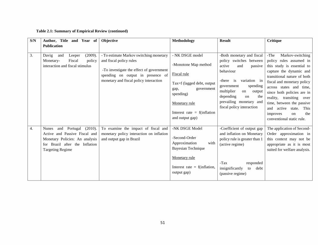
51
Table 2.1: Summary of Empirical Review (continued)
S/N Author, Title and Year of
Publication
Objective Methodology Result Critique
3. Davig and Leeper (2009).
Monetary- Fiscal policy
interaction and fiscal stimulus
- To estimate Markov switching monetary
and fiscal policy rules
-To investigate the effect of government
spending on output in presence of
monetary and fiscal policy interaction
- NK DSGE model
-Monotone Map method
Fiscal rule
Tax=f (lagged debt, output
gap, government
spending)
Monetary rule
Interest rate = f(inflation
and output gap)
-Both monetary and fiscal
policy switches between
active and passive
behaviour
-there is variation in
government spending
multiplier on output
depending on the
prevailing monetary and
fiscal policy interaction
-The Markov-switching
policy rules assumed in
this study is essential to
capture the dynamic and
transitional nature of both
fiscal and monetary policy
across states and time,
since both policies are in
reality, transiting over
time, between the passive
and active state. This
improves on the
conventional static rule.
4.
Nunes and Portugal (2010).
Active and Passive Fiscal and
Monetary Policies: An analysis
for Brazil after the Inflation
Targeting Regime
To examine the impact of fiscal and
monetary policy interaction on inflation
and output gap in Brazil
-NK DSGE Model
-Second-Order
Approximation with
Bayesian Technique
Monetary rule
Interest rate = f(inflation,
output gap)
-Coefficient of output gap
and inflation on Monetary
policy rule is greater than 1
(active regime)
-Tax responded
insignificantly to debt
(passive regime)
The application of Second-
Order approximation in
this context may not be
appropriate as it is most
suited for welfare analysis.
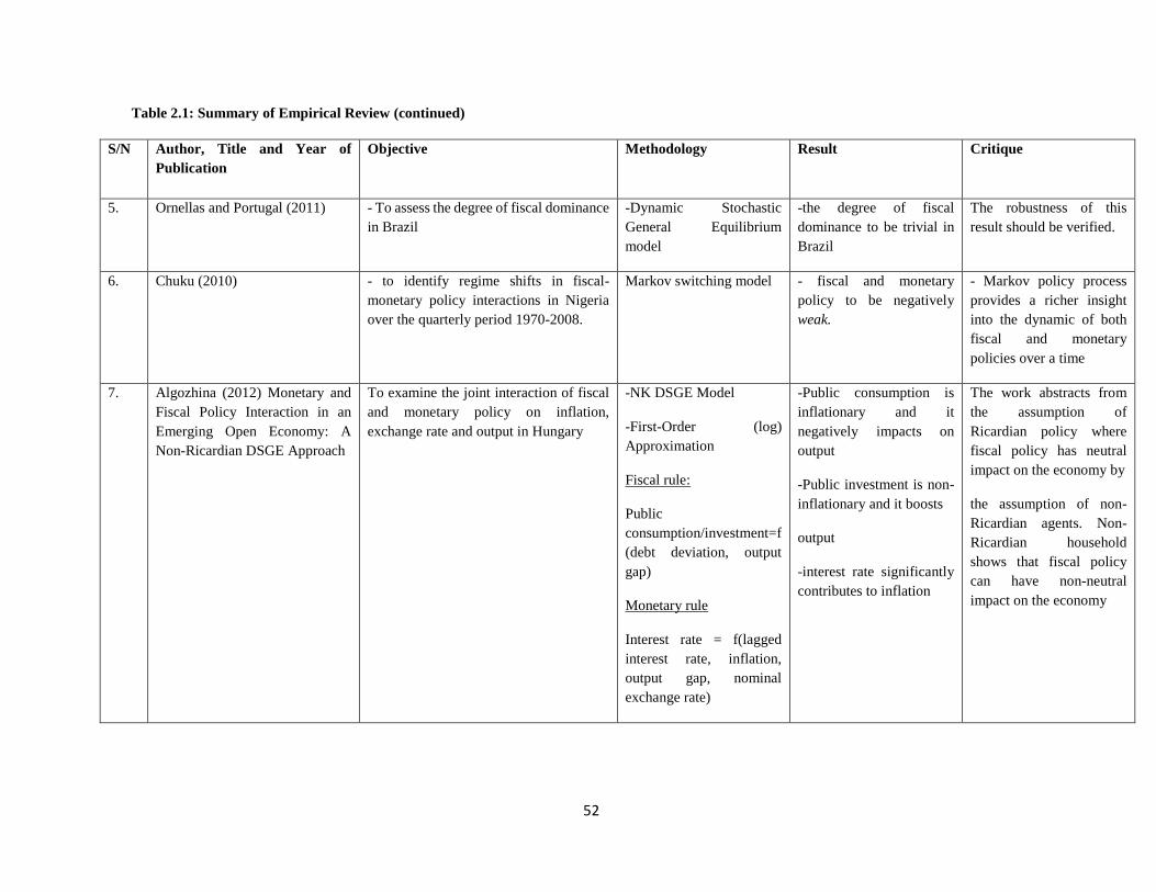
52
Table 2.1: Summary of Empirical Review (continued)
S/N Author, Title and Year of
Publication
Objective Methodology Result Critique
5. Ornellas and Portugal (2011) - To assess the degree of fiscal dominance
in Brazil
-Dynamic Stochastic
General Equilibrium
model
-the degree of fiscal
dominance to be trivial in
Brazil
The robustness of this
result should be verified.
6. Chuku (2010) - to identify regime shifts in fiscal-
monetary policy interactions in Nigeria
over the quarterly period 1970-2008.
Markov switching model - fiscal and monetary
policy to be negatively
weak.
- Markov policy process
provides a richer insight
into the dynamic of both
fiscal and monetary
policies over a time
7. Algozhina (2012) Monetary and
Fiscal Policy Interaction in an
Emerging Open Economy: A
Non-Ricardian DSGE Approach
To examine the joint interaction of fiscal
and monetary policy on inflation,
exchange rate and output in Hungary
-NK DSGE Model
-First-Order (log)
Approximation
Fiscal rule:
Public
consumption/investment=f
(debt deviation, output
gap)
Monetary rule
Interest rate = f(lagged
interest rate, inflation,
output gap, nominal
exchange rate)
-Public consumption is
inflationary and it
negatively impacts on
output
-Public investment is non-
inflationary and it boosts
output
-interest rate significantly
contributes to inflation
The work abstracts from
the assumption of
Ricardian policy where
fiscal policy has neutral
impact on the economy by
the assumption of non-
Ricardian agents. Non-
Ricardian household
shows that fiscal policy
can have non-neutral
impact on the economy

53
Table 2.1: Summary of Empirical Review (continued)
S/N Author, Title and Year of
Publication
Objective Methodology Result Critique
8. Lima, Maka and Pumar (2012) - To determine the interactions between
fiscal and monetary policy in Brazil.
SVAR model They use two different
identification schemes that
produce inconsistent result
in deciding the existence
of fiscal dominance or not
in Brazil
-the shock identification
scheme fails to produce a
robust result. There is need
for further studies to
handle the inconsistency
9. Anas (2013). Monetary and
Fiscal Policy in an Estimated
DSGE Model for Morocco
To assess the effect of monetary and
fiscal policy on macroeconomic
outcomes such as inflation and output in
Morocco
RBC Model
-First-Order
Approximation
-Bayesian Technique
Fiscal rule
Tax=f(lagged debt,
government spending,
inflation, output, interest
rate)
Monetary rule
Interest rate = f(inflation,
output gap)
-shock to interest rate
impacts negatively on
output and inflation
-shock to capital tax
reduces investment and
output
-shock to government
spending raises output
-New Keynesian DSGE
models are better suited for
economic policy analysis
when compared to the Real
Business cycle models.

54
Table 2.1: Summary of Empirical Review (continued)
S/N Author, Title and Year of
Publication
Objective Methodology Result Critique
10. Cekin (2013). Monetary and
Fiscal Policy Interaction in
Turkey: A Markov Switch
Approach
-characterised monetary and fiscal
policies in Turkey with Markov
Switching simple policy rules for the
periods before and after 2001
-To determine the effect of fiscal-
monetary policy interaction on price level
in Turkey
-DSGE Model
-First-Order (log)
Approximation
Fiscal rule
Tax=f(government
spending, output gap and
lagged debt)
Budget deficit = f (lagged
debt, government
spending, measure of
business cycle fluctuation)
Monetary rule
Interest rate = f(inflation,
output gap, exchange rate)
- both monetary and fiscal
policies switched over
time between active and
passive regimes
-active monetary policy
and passive fiscal policy
led to stable inflation
-The Markov switching
model allows one to
identify regime shifts in
the nature of economic
policies over time
11. Gonzalez-Astudillo (2013).
Monetary-Fiscal Policy
Interaction: Interdependent
Policy Rule Coefficient
To determine coordinated fiscal and
monetary policy rules that impact on
inflation and output in the United States
-NK DSGE Model
--Bayesian Technique
Fiscal rule
Tax=f(debt deviation,
output gap)
Monetary rule
Interest rate = f(inflation,
output gap)
-both fiscal and monetary
policy switch between
active and passive regimes
-shocks to both tax and
interest rate reduce
inflation and output in the
short-run
The work shows that fiscal
and monetary policy rules
can be dynamic and their
innovations can be
modelled as being serially
correlated
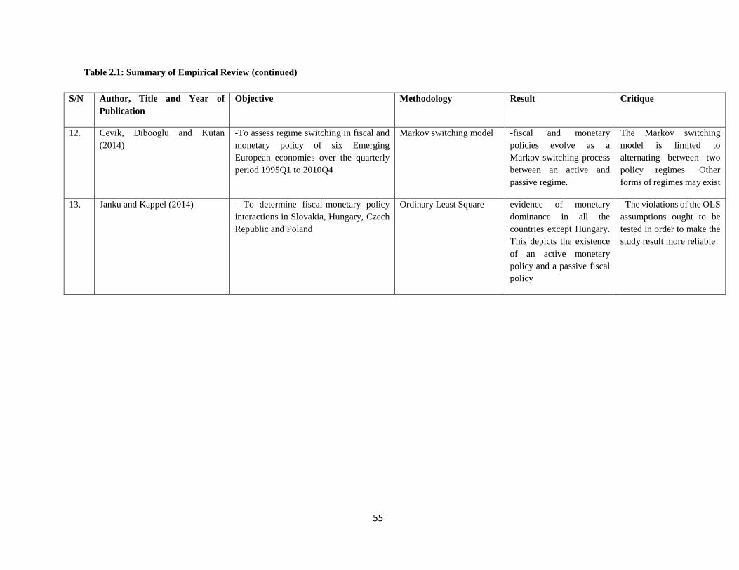
55
Table 2.1: Summary of Empirical Review (continued)
S/N Author, Title and Year of
Publication
Objective Methodology Result Critique
12. Cevik, Dibooglu and Kutan
(2014)
-To assess regime switching in fiscal and
monetary policy of six Emerging
European economies over the quarterly
period 1995Q1 to 2010Q4
Markov switching model -fiscal and monetary
policies evolve as a
Markov switching process
between an active and
passive regime.
The Markov switching
model is limited to
alternating between two
policy regimes. Other
forms of regimes may exist
13. Janku and Kappel (2014) - To determine fiscal-monetary policy
interactions in Slovakia, Hungary, Czech
Republic and Poland
Ordinary Least Square evidence of monetary
dominance in all the
countries except Hungary.
This depicts the existence
of an active monetary
policy and a passive fiscal
policy
- The violations of the OLS
assumptions ought to be
tested in order to make the
study result more reliable
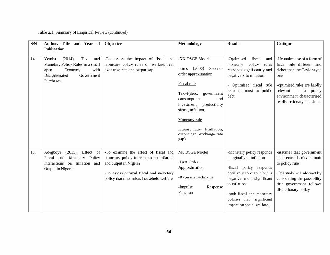
56
Table 2.1: Summary of Empirical Review (continued)
S/N Author, Title and Year of
Publication
Objective Methodology Result Critique
14.
Yemba (2014). Tax and
Monetary Policy Rules in a small
open Economy with
Disaggregated Government
Purchases
-To assess the impact of fiscal and
monetary policy rules on welfare, real
exchange rate and output gap
-NK DSGE Model
-Sims (2000) Second-
order approximation
Fiscal rule
Tax=f(debt, government
consumption and
investment, productivity
shock, inflation)
Monetary rule
Interest rate= f(inflation,
output gap, exchange rate
gap)
-Optimised fiscal and
monetary policy rules
responds significantly and
negatively to inflation
- Optimised fiscal rule
responds most to public
debt
-He makes use of a form of
fiscal rule different and
richer than the Taylor-type
one
-optimised rules are hardly
relevant in a policy
environment characterised
by discretionary decisions
15. Adegboye (2015). Effect of
Fiscal and Monetary Policy
Interactions on Inflation and
Output in Nigeria
-To examine the effect of fiscal and
monetary policy interaction on inflation
and output in Nigeria
-To assess optimal fiscal and monetary
policy that maximises household welfare
NK DSGE Model
-First-Order
Approximation
-Bayesian Technique
-Impulse Response
Function
-Monetary policy responds
marginally to inflation.
-fiscal policy responds
positively to output but is
negative and insignificant
to inflation.
-both fiscal and monetary
policies had significant
impact on social welfare.
-assumes that government
and central banks commit
to policy rule
This study will abstract by
considering the possibility
that government follows
discretionary policy

57
Table 2.1: Summary of Empirical Review (continued)
16. Cazacu (2015) To examine fiscal and monetary policy
interactions in Romania
Structural VAR model - No distinct pattern of
interactions between fiscal
and monetary policies over
the quarterly period
2000Q1 to 2014Q2.
This may be sensitive to
the shock identification
scheme adopted.
Robustness of the result
should be conducted
17. Dimakou (2015) To assess fiscal-monetary policy
interaction in the face of bureaucratic
corruption by public officials on 77
developed and developing countries
-event study analysis
-Panel data analysis
Corrupt activities have a
significant impact in
affecting government’
fiscal decisions, which can
undermine the Central
Bank’s ability to control
inflation.
The argument of this study
is relevant in the context of
developing economies.
The Dynamic Stochastic
General Equilibrium
framework can also be
used to examine and to
provide a richer context to
examine the thesis of the
study
S/N Author, Title and Year of
Publication
Objective Methodology Result Critique

58
Table 2.1: Summary of Empirical Review (continued)
18. Jawadi, Mallick and Sousa (2016) To examine the macroeconomic effects of
fiscal and monetary policies in five
emerging economies. They also
characterise the existing nature of fiscal
and monetary interrelation in these
economies.
Panel Vector
Autoregressive method
They find that monetary
and fiscal policies have
respectively, negative and
positive effects on the
aggregate economy. At the
same time, both fiscal and
monetary policy interacts
as complements.
This study can also be
examined using a multi-
country Dynamic
Stochastic General
Equilibrium model. This
will help to complement
the existing result
19.. Gilksberg (2016) To investigate the joint fiscal and
monetary policy rules that guarantees a
unique solution to a dynamic general
equilibrium model.
Numerical simulation of
Dynamic General
Equilibrium model
finds that three forms of
fiscal-monetary
interactions deliver a
unique rational
expectations equilibrium.
These include active fiscal,
passive monetary
combination, active
monetary and passive
fiscal combination and a
passive fiscal and passive
monetary regime.
The passive fiscal and
passive monetary regime is
a novel finding different
from Leeper (1991)
conventional prescription
of an active and passive
combination.
S/N Author, Title and Year of
Publication
Objective Methodology Result Critique
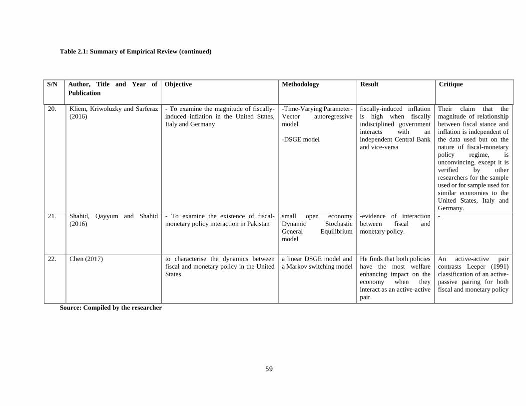
59
Table 2.1: Summary of Empirical Review (continued)
20. Kliem, Kriwoluzky and Sarferaz
(2016)
- To examine the magnitude of fiscally-
induced inflation in the United States,
Italy and Germany
-Time-Varying Parameter-
Vector autoregressive
model
-DSGE model
fiscally-induced inflation
is high when fiscally
indisciplined government
interacts with an
independent Central Bank
and vice-versa
Their claim that the
magnitude of relationship
between fiscal stance and
inflation is independent of
the data used but on the
nature of fiscal-monetary
policy regime, is
unconvincing, except it is
verified by other
researchers for the sample
used or for sample used for
similar economies to the
United States, Italy and
Germany.
21. Shahid, Qayyum and Shahid
(2016)
- To examine the existence of fiscal-
monetary policy interaction in Pakistan
small open economy
Dynamic Stochastic
General Equilibrium
model
-evidence of interaction
between fiscal and
monetary policy.
-
22. Chen (2017) to characterise the dynamics between
fiscal and monetary policy in the United
States
a linear DSGE model and
a Markov switching model
He finds that both policies
have the most welfare
enhancing impact on the
economy when they
interact as an active-active
pair.
An active-active pair
contrasts Leeper (1991)
classification of an active-
passive pairing for both
fiscal and monetary policy
Source: Compiled by the researcher
S/N Author, Title and Year of
Publication
Objective Methodology Result Critique
i
2.7 Summary of Identified Gaps in the Literature
This section presented the definitional, theoretical, methodological and empirical review of the
literature on fiscal and monetary policy interactions.
In the definitional review, fiscal and monetary policy interactions in the context of this study were
defined. In the theoretical review, the major theories of fiscal and monetary policy interactions
were outlined and critiqued. From the methodological review, one finds that the a-theoretic, game-
theoretic and dynamic general equilibrium frameworks have been used to investigate fiscal-
monetary policy interactions. The empirical review showed mixed evidence on the interaction
between fiscal and monetary policy and their impact on macroeconomic variables such as inflation
and output gap, across different economies.
Finally, the following research gaps can be deduced from the literature reviewed:
1. The study of fiscal and monetary policy interaction in Nigeria is a nascent one. The few studies
on fiscal and monetary policy interaction in Nigeria include Chuku (2010); Okafor (2013);
Englama et al., (2013); Musa et al., (2013). Furthermore, these studies employ a-theoretic
estimation techniques. For instance, Englama et al., (2013); Musa, Asare and Gulumbe (2013)
investigate fiscal and monetary policy interaction in Nigeria using the cointegration technique
while Chuku (2010) use a Markov switch state-space method.
2. There is also sparseness in articles that examined fiscal and monetary policy interaction within
micro-founded models of the dynamic general equilibrium framework in Nigeria. Adegboye
(2015) is one of few studies that investigate the effect of fiscal and monetary policy interactions
on inflation and output in Nigeria, within a dynamic general equilibrium framework. One reason
for this sparseness is that dynamic general equilibrium modelling in Nigeria is a recent venture
and only few studies such as Olekah and Oyaromade (2007), Olayeni, (2009), Alege, (2008, 2012),
Garcia (2009), and Adebiyi and Mordi (2010) exist.
This study however, adapts the models used in these existing works to examine fiscal and monetary
policy interactions in Nigeria. For example, Alege (2008, 2012) conducts macroeconomic policy
analysis within a DSGE model. The study considers the interaction of monetary, financial and
ii
export policies, but omits both the fiscal sector and assumptions of a small open economy that is
interacting with the rest of the world. This current study will address these omissions.
3. Most studies on fiscal and monetary policy interaction in DSGE model assume that government
is a benevolent entity that commits to a policy rule and that fiscal and monetary policy are fully
coordinated. These assumptions may be unrealistic for a developing country such as Nigeria. These
assumptions are, therefore, modified in the context of a developing economy.
4. Most studies on fiscal and monetary policy interaction in DSGE model rely on an implicit
definition of policy interaction. This is because the DSGE framework provides a natural setting to
consider policy interactions, since it implicitly assumes the existence of simultaneous interactions
among economic agents, that is, households, firms, central bank and government. This study
argues that the implicit interaction does not capture the combined effect of both policies on
inflation and output. The study, however, constructs an interaction variable to explicitly capture
the interrelationship between fiscal and monetary policies and to quantify the combined policy
interactions.
iii
CHAPTER THREE
STYLISED FACTS
In this chapter, stylised facts that depict the empirical regularities surrounding the interaction
among major economic variables in the context of this study are presented. The chapter is divided
into five sections. In Section 3.1, the structure of the Nigerian economy is examined. The fiscal
and monetary policy frameworks that exist in Nigeria are outlined in Section 3.2 and thereafter, a
trend and business cycle analysis on relevant fiscal and monetary variables vis-à-vis
macroeconomic outcomes is performed in order to generate relevant preliminary facts in Section
3.3 and Section 3.4. In Section 3.5, empirical facts on the alternative assumptions used in this study
are presented.
3.1 Structure of the Nigerian Economy
The structure of a national economy is multifaceted. In a broad sense, it encompasses an
interrelated system- institutional, demographic, geographical, etc- through which activities in an
economy are coordinated (Anyanwu, 1997). But in a narrow sense, it outlines the patterns and
composition of relevant sectors as they determine performance in an economy over a period. In
other words, it presents the patterns and composition of consumption, employment, trade and most
essentially the production base in an economy.
By production base, many national economies are divided into three: the primary, secondary and
tertiary sectors. The economy of Nigeria, in the same vein, is structurally divided into these three
sectors. The primary sector comprises productive activities related to natural resources and
includes agriculture, mining and quarrying while productive activities in the secondary sector
consists of processing primary commodities. It includes manufacturing, building and construction.
Essentially, services ranging from transport, communication and finance belong to the tertiary
sector. This classification is depicted in Table 3.1.
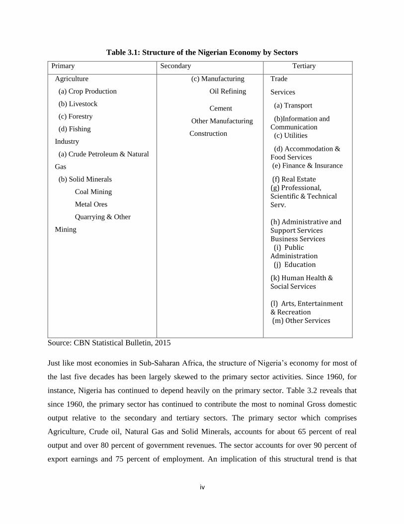
iv
Table 3.1: Structure of the Nigerian Economy by Sectors
Primary Secondary Tertiary
Agriculture
(a) Crop Production
(b) Livestock
(c) Forestry
(d) Fishing
Industry
(a) Crude Petroleum & Natural
Gas
(b) Solid Minerals
Coal Mining
Metal Ores
Quarrying & Other
Mining
(c) Manufacturing
Oil Refining
Cement
Other Manufacturing
Construction
Trade
Services
(a) Transport
(b)Information and
Communication
(c) Utilities
(d) Accommodation &
Food Services
(e) Finance & Insurance
(f) Real Estate (g) Professional, Scientific & Technical Serv. (h) Administrative and Support Services Business Services (i) Public Administration (j) Education
(k) Human Health & Social Services (l) Arts, Entertainment & Recreation (m) Other Services
Source: CBN Statistical Bulletin, 2015
Just like most economies in Sub-Saharan Africa, the structure of Nigeria’s economy for most of
the last five decades has been largely skewed to the primary sector activities. Since 1960, for
instance, Nigeria has continued to depend heavily on the primary sector. Table 3.2 reveals that
since 1960, the primary sector has continued to contribute the most to nominal Gross domestic
output relative to the secondary and tertiary sectors. The primary sector which comprises
Agriculture, Crude oil, Natural Gas and Solid Minerals, accounts for about 65 percent of real
output and over 80 percent of government revenues. The sector accounts for over 90 percent of
export earnings and 75 percent of employment. An implication of this structural trend is that
v
Nigeria has a narrowly diversified and externally oriented productive base that makes her
vulnerable to external shocks due to volatility in prices of primary commodities in the international
market.
Trends in the secondary sector comprising manufacturing and building subsectors as seen in Table
3.2 are unimpressive. Specifically, the sectoral contribution of this sector to GDP has consistently
declined on average from 15.6 per cent in the 1970s to 5.7 per cent in the period, 2001-2009. This
trend suggests that Nigeria has experienced a process of de-industrialization since the 1970s. Also,
one may argue that structural transformation of the economy from the primary to secondary sector
is slow or non-existent.
By contrast the contribution of the service sector to nominal output has been on the rise for over
three decades. In the 1980s, the service sector contributed an average of 24.3 per cent rising to
29.5 per cent in the 2000s. The favourable trend can be explained by several reasons varying from
the entry of telecommunications companies, the rise of information and communication
technology and increased sophisticated banking and financial services among others. However,
with the rebasing of the Nigerian economy in 2014, there has been a dramatic structural change in
the economy. The tertiary sector in the period 2010-2015 contributed the most to real output,
making up to 52.0 per cent, the primary sector followed at 36.1 per cent and the secondary sector
comprising manufacturing and construction constituted the least productive sector at 11.8 per cent.

vi
Table 3.2: Sectoral Contributions to GDP (in percent)
Sources: Sanusi (2010) and CBN Statistical Bulletin, 2015+
Note: * Re-based GDP
Considering the structure of the Nigerian economy from the stance of the primary, secondary and
tertiary sector alone is incomplete. One can also structurally divide the economy into the oil and
non-oil sectors, although this is a broad classification and is liable to becloud some specific details
about the economy. This classification is relevant in light of the economy’s heavy reliance on the
crude oil sector. From statistics presented in Table 3.3, the oil sector contributes less to total output
relative to the non-oil sector. This is due to the weak linkage of the oil sector to the other sectors
of the economy, in terms of its low value-addition. The irony is that the oil sector generates more
revenue for the Nigerian economy, despite its miniature contribution to total output.
Activity Sector 1960-
1970
1971-
1980
1981-
1990
1991-
2000
2001-
2009
2010-
2015*+
Primary sector
Agriculture
Crude oil, gas
and solid
minerals
Total Primary
Secondary
Manufacturing
Building and
Construction
Total
Secondary
Tertiary
Wholesale and
Retail Trade
Services
Total Tertiary
55.8
11.3
67.1
6.6
4.8
11.4
12.8
15.3
28.1
28.4
29.1
57.5
7.3
8.3
15.6
17.6
16.5
34.1
32.3
41.0
73.5
6.1
2.3
8.4
14.5
9.8
24.3
34.2
38.6
72.8
4.9
1.8
6.7
13.8
11.5
25.3
40.3
28.4
68.7
3.9
1.8
5.7
14.0
15.5
29.5
23.4
12.7
36.1
8.4
3.4
11.8
16.6
35.4
52.0

vii
Table 3.3: Oil and Non-oil contribution to GDP (in percent)
Activity
Sector
1960 1970 1980 1990 2000 2010 2015+
Oil sector
Non-oil sector
0.44
99.56
11.04
88.96
21.41
78.51
37.46
62.54
32.45
67.55
15.88
84.12
9.60
90.39
Sources: Sanusi (2010) and CBN Statistical Bulletin, 2015+
3.2 Monetary and Fiscal Policy in the Nigerian Economy
3.2.1 Monetary Policy in Nigeria
Monetary policy is the combination of measures designed to control the level of money supply,
interest rates and credit in an economy in tandem with the desired level of economic activity. The
fundamental goals of monetary policy are attainment of low inflation and sustainable economic
growth. Other objectives include full employment and stable real exchange rates. In Nigeria, The
Central Bank of Nigeria (CBN) is charged with the formulation and conduct of monetary policy
(Central Bank of Nigeria Act 1958, 1991 and 2007). Its monetary policy thrust is to control money
supply and interest rates in order to achieve the ultimate goals of price stability and economic
growth (Central Bank of Nigeria, 2011a).
Since 1959, the monetary policy of the Central Bank of Nigeria has been conducted under two
divergent frameworks. These are the exchange rate targeting and monetary targeting regimes. The
exchange rate framework was used between 1959 and 1974. Under this regime, the value of
Nigeria’s currency was pegged to the British pound, then to the American dollars and afterwards
to a basket comprising the currencies of twelve Nigeria’s major trading partners. An advantage of
the exchange rate framework is that it provides an easily monitored nominal anchor to guide price
stability. However, in the face of excessive monetary expansions and fiscal dominance, this
framework can lead to increased inflationary pressures that erode international competitiveness
and create current account imbalances (Mason, 2006). In Nigeria, the collapse of the Bretton
Woods system of fixed exchange rates in 1974 and a change in strategy to demand management
as a means of containing inflationary pressures and balance of payments imbalances posed
challenges to the effectiveness of the exchange rate targeting framework (Central Bank of Nigeria,
2011a).

viii
The CBN, by 1974, transited to the monetary targeting framework. The monetary targeting regime
entails directly controlling monetary aggregates such as the money base in order to control
inflationary pressures. It remains the current monetary policy framework of the CBN. Unlike the
exchange rate targeting, the monetary targeting framework allows monetary policy to focus on
internal or domestic issues (Mishkin, 2000). This framework is effective on the argument that the
relationship between monetary aggregates and macroeconomic outcomes such as output and
inflation is stable. In this regard, Agu (2007) demonstrates that monetary aggregates have indeed
been fairly stable and is an effective tool of monetary policy in Nigeria. Furthermore, this
framework has continued to be applicable because of its suitability with relatively undeveloped
financial markets. Alongside the use of monetary targets, the CBN has also implicitly adopted an
interest rate target. Under this framework, an interest rate serves as the anchor for setting other
interest rates in the economy. However, with continued evolvement of the financial market and
economic policy environments, there are indications that Nigeria may transit to an inflation
targeting regime as currently used by many developed economies.
A second dimension of the monetary policy framework of the CBN can also be classified as the
adoption of direct or non-market-based instruments (1974-1993) and indirect or market-based
instruments (1993-date). Before the implementation of the Structural Adjustment Program in 1986
and with the existence of underdeveloped money and capital markets, monetary policy was
conducted using direct control. Instruments used in this regime included credit ceilings to deposit
money banks, sectoral credit allocation to priority sectors of the economy, interest rate and
exchange rate control. With the introduction of the Structural Adjustment Program in 1986, there
was a gradual shift to the indirect control or market-based regime. This began with the elimination
of credit ceiling imposed on some banks and then, the adoption of the Open market operations in
1993 as the major instrument. Other instruments adopted under this regime include reserve
requirements and discount window operations.
Following the implicit adoption of an interest rate target by the Central Bank of Nigeria, the
Minimum Rediscount Rate (MRR) was adopted as the anchor rate. However, in December 2006,
CBN used adopted the Monetary Policy Rate in place of the Minimum Rediscount Rate, in order
to eliminate interest rate volatility and to tackle the unresponsiveness of the MRR to the policy

ix
actions of the apex bank (CBN Monetary Policy Committee Communique No. 48, 2006). Under
this framework, CBN introduced the standing deposit and lending facility that allowed Discount
Houses and Deposit Money Banks that need funds to address their liquidity shortages while those
with excess liquidity can deposit the funds overnight.
A third dimension to the monetary policy framework of the CBN entails the use of a short-term
framework or medium-term framework. The short-term framework is an annual framework used
between 1986 till 2001. In 2002, the CBN transited to a medium-term framework, which is a bi-
annual framework, in the implementation of monetary policy. This most recent framework is
hinged on the assumption that monetary policy actions affects ultimate economic goals with a lag.
An advantage of the medium-term framework is that it addresses the challenge of time
inconsistency in the implementation of monetary policy (Central Bank of Nigeria, 2015a).
Another aspect of monetary policy concerns its transmission channel to the economy. With regard
to this, the major channels in Nigeria are through money aggregates and interest rate. The first
channel entails setting an operating target using the base money through an intermediate target,
the broad money supply (M2). Under this channel, the CBN uses the Open Market Operation
(OMO) to transact financial securities with both banks and non-bank public for the purpose of
influencing the ability of banks to create money. This invariably affects the level of money
supplied in the economy. The second channel involves setting an anchor interest rate whose value
influences expectation of the private sector and then, affects financial asset prices and exchange
rate.
3.2.2 Fiscal Policy in Nigeria
Fiscal policy in Nigeria is largely intertwined within fiscal federalism- an intergovernmental fiscal
relationship existing among the various tiers of government. In a fiscal federalist state, there exists
more than one tier of government where each has different expenditure and revenue raising
powers. The various fiscal tools that are implemented are guided by the existing fiscal federalist
structure, as contained in the Nigerian constitutions, development plans and specific frameworks
such as the Fiscal Responsibility Act of 2007.

x
The various Nigerian Constitutions explicitly allocates taxation and expenditure power among the
existing tiers of government. For instance, the Richard Constitution of 1946 divided Nigeria into
the Northern, Western and Eastern regions alongside the Federal Government. Under this era, the
Philipson Commission appointed to assign fiscal and administrative duties to the regional
governments, stipulated that regional governments be entitled to revenues that included personal
income tax, property tax, licenses, etc while revenue accruing to the federal government was to be
shared using the derivation principle. The Philipson Commission arrangement was discarded as
the Richard Constitution of 1946 was replaced by the Macpherson Constitution of 1951.
Under the Macpherson Constitution of 1951, the Macpherson Arrangements, Hicks Philipson
Commission, Chick Commission and Raisman Commission were appointed respectively. Some
important fiscal reviews under these regimes include the allocation of more taxing power to the
regional government. The Raisman commission also created a distributable pool account where a
certain per cent of federally-collected revenue was paid and shared among the regions using the
sharing formula: 40 per cent to the North, 31 per cent to the East, 24 per cent to the West and 5
per cent to Southern Cameroon. The Macpherson Constitution of 1951 was replaced by the 1960
Constitution and then, the 1963 Constitution, when Nigeria became a Republic. Under the 1963
Constitution, the Binns Commission was created to review existing fiscal procedures. The Binns
Commission recommended an increase of federal contribution to the distributable pool account
from 30 to 35 per cent. With the creation of a fourth region, the Mid Western region, the revenue
sharing formula was also reviewed.
A slight change to the federal structure occurred after the military government seized power in
1966. The four regions were transformed into a 12-state structure by General Yakubu Gowon in
1967. Under the military regimes, various decrees were promulgated to determine fiscal
responsibilities and powers among the states and central government. For example, Decree No.13
of 1970 adopted population and equality of states as revenue sharing formula. Other reputable
commissions adopted include the Aboyade Technical Committee on Revenue Allocation and the
Okigbo Commission. Also, the current 1999 Constitution provides a framework that guide
government’s fiscal actions. For instance, expenditure responsibility is assigned among the various

xi
level of government as contained in the exclusive, concurrent legislative list, the residual list and
the establishment of local government.
Tables 3.4 and 3.5 illustrate the allocation of tax and expenditure powers among the three tiers of
government- Federal, State and Local- in Nigeria. It can be implied from Table 3.4 that the Federal
Government collects revenue from major sources such as the Import and Excise duties, Mining
rents and royalties; and the petroleum profits tax, while the State and Local Government have
jurisdiction over low yielding sources. The Federal Government is, then, able to raise more revenue
to meet its expenses (Anyanwu, 1999).
Table 3.4: Tax Jurisdiction in Nigeria
Federal State Local
Import Tariffs
Excise duties
Export duties
Mining rents and
royalties
Petroleum profits tax
Companies income tax
Capital gains tax
Personal income tax
Value added tax
Football pools and other betting
taxes
Entertainment taxes and estate
duties
Gift tax
Land tax
Land registration fees
Capital gains tax
Personal income tax
Stamp duties
Rates
Tenement rate
Market and trading licenses
and fees
Motor park duties
Advertisement fees
Entertainment tax
Radio/television licenses
Sources: Nigerian Constitution (1999), Olayiwola and Osabuhien (2011)

xii
Table 3.5: Expenditure Responsibilities in Nigeria
Federal only Federal-State
(shared)
State only Local government only
-Defence
-Foreign affairs
-International trade
including export
marketing
-Currency, banking,
borrowing,
exchange control
-Use of water
resources
-Shipping, federal
trunk roads
-Elections
-Aviation, railways,
postal services
-Business
registration
-Price control, etc
-Health, social
welfare
-Education (post
primary/technology
)
-Culture
-Antiquities
-Monuments,
archives
-Statistics, stamp
duties
-Commerce,
industry
-Electricity
-Research surveys
Residual power
i.e. any subject
not assigned to
federal or local
government by
the constitution
-Economic Planning
-Health services
-Land use
-Control and regulation
of advertisements, pets,
small businesses
-Market, public
conveniences
-Social welfare, sewage
and refuse disposal,
registration of births,
deaths
-Marriages
-Primary, adults and
vocational education
-Development of
agriculture and natural
resources
Source: Nigerian Constitution (1999)
A second channel by which fiscal policy in Nigeria is planned and implemented is through the
Development Plans. The development plans are useful in delineating fiscal policies in Nigeria.
Nigeria has, over the decades, adopted various forms of development planning ranging from long
term, medium term, short range, perspective plans and rolling plans (Anyanwu, Oyefusi,
Oaikhenan and Dimowo, 1997). In these plans, government projected expenditure strategies are
usually outlined. Development planning in Nigeria began with the Ten-Year plan of Development
and Welfare (1945-1955) and the Second Plan (1955-1960) in the colonial era. Furthermore, in the
post-independence era, there have been four National Developments (1962-1968; 1970-1974,
1975-1980 and 1981-1985), five rolling plans (1990-1992,1991-1993, 1993-1995, 1994-1996 and
1997-1999), medium term plans: National Economic Empowerment and Development Strategies
(NEEDS I and II) and Vision 2020 as a perspective plan. Some of the policy thrusts of these plans
are summarised in Anyanwu et al., (1997) as: generating significant additional revenue,
diversification of the revenue base, achieve macroeconomic stability, attain job creation and
employment opportunities, promote self-reliant development among others
xiii
The conduct of fiscal policy in Nigeria can also be deciphered by specific frameworks such as the
Fiscal Responsibility Act of 2007. The Medium Term Expenditure Framework (MTEF) sprang
from this act. The MTEF is a three-year rolling plan which articulates government’s proposed
expenditure and revenue and its fiscal policy goals. It comprises a macroeconomic framework, a
fiscal strategy paper, expenditure and revenue framework, consolidated debt statement and
statement of contingent liability (Fiscal Responsibility Act, 2007). Furthermore, the MTEF serves
as a framework for preparing the annual budgets. Some examples of MTEF include: 2009-2011,
2011-2013, 2013-2015, 2014-2016 and currently, 2015-2017. Recently, the Federal Government
launched the Economic Recovery Growth Plan (ERGP), a medium- term plan for the period 2017-
2020 (Ministry of Budget and National Planning, 2017). This plan is geared towards resuscitating
the Nigerian economy after a short bout of recession, investing in the human capital base of Nigeria
and enhancing the global competitiveness of the nation.
Lastly, the annual budget is the fourth framework that has been used to guide fiscal policy in
Nigeria. In Table 3.6, the annual budget projections for some selected years are presented.

xiv
Table 3.6: Nigerian Annual Budgets Year Thrust Revenue
( N’billion)
Expenditure
( N’billion)
Fiscal
deficit as
% of GDP
Debt service
( N’billion)
2000 -reduce inflationary trend
-provide enabling factors for
private-sector led economic growth
-improve education and
agricultural production
-reduce unemployment
Total revenue-
1,686
Oil revenue-
1, 340
Non-oil
revenue- 345.6
Capital expenditure-
31.6;
Recurrent
expenditure- 341.53
- Domestic debt
servicing- 100
External debt
servicing- 150
2003 Embark on a growth strategy that
would achieve fiscal stability;
improve non-oil sector
competitiveness; reduce inflation;
maintain a fiscal deficit not
exceeding 2.5 percent of GDP
685.4
Total expenditure –
765.1
Recurrent
expenditure- 508.8
Capital expenditure-
256.4
- External debt
servicing- 252
2014 Continuation of prudent economic
management in order to build on
recent economic growth to support
job creation and more
infrastructure
3,730 4,642
Recurrent (non-debt)
2,430
Capital 1,101
Debt service 712
Statutory transfers
399
1.90
percent
712
2015
Described as “A Transition
Budget”, that focuses on managing
the declining revenue and
transiting to a non-oil based
economy.
3,602
Recurrent (non-debt)
2,616
Capital (including
SURE P) 634
Debt service 943
Statutory transfers
412
Subsidy reinvestment
program (SURE P)
103
Aggregate
0.7 percent
943
2017 Budget of Economic Recovery 4,940 Expenditure 4,358
Recurrent- 2,980
Capital- 2,240
Total- 7.289
2.18
percent
1,841.3
Source: Central Bank of Nigeria (2015b) and Budget Office of the Federation (2017)

xv
3.2.3 Monetary and Fiscal Policy Coordination in Nigeria
The Central Bank of Nigeria and the Federal Ministry of Finance are two independent bodies in
charge of respectively conducting monetary and fiscal policy in Nigeria. However, by the Central
Bank of Nigeria (CBN) Act of 2007, the CBN is granted operational independence to direct
monetary policy using policy instruments and variables such as the policy rates and broad money
supply. Its primary macroeconomic objective is to attain price stability. Conversely, the Federal
Ministry of Finance (FMF) alongside adjunct parastatals such as the Debt Management Office
(DMO) oversees fiscal policy using instruments such as taxes and expenditure, usually with the
focal objective of long term economic growth and fiscal policy sustainability.
Often times conflicts and externalities arise when monetary and fiscal policy variables and targets
are independently set and implemented which threatens the internal consistency in the
macroeconomy and leads to suboptimal policy outcomes (Garba, 2004). As a result, there is need
to harmonise both policies, necessitating the existence of both institutional and operational
frameworks for harmonising these policies in Nigeria.
Institutional Framework of Policy Coordination in Nigeria
The institutional framework creates avenue for joint decision making between the Central Bank of
Nigeria and the Federal Ministry of Finance through formal or informal committees. Firstly, on a
high level, the joint decision making occurs through a bilateral interaction between head of the
fiscal and monetary institutions. Secondly, the joint interaction takes place with formal committee
meeting. Some of them include: The Fiscal Liquidity Assessment Committee (FLAC) of the CBN,
Monetary and Fiscal Policy Coordinating Committee (MFPCC) of the DMO and Cash
Management Committee of the Federal Ministry of Finance. FLAC comprise of members from
Federal Ministry of Finance, Debt Management Office (DMO), Office of the Accountant- General
of the Federation (OAGF), Budget Office of the Federation (BOF), Nigerian National Petroleum
Corporation (NNPC), Nigeria Customs Service (NCS), Federal Inland Revenue Service (FIRS),
the Department of Petroleum Resources (DPR) and relevant departments of the Central Bank of
Nigeria, who meet weekly to deliberate on the government fiscal operates affects CBN’s goal of
price stability. FLAC has developed a database on the operations of the relevant MDAs and a
xvi
template for forecasting the Treasury’s operations as input to the Bank’s Liquidity Assessment
Model (Central Bank of Nigeria, 2011b).
Secondly, the Monetary and Fiscal Policy Coordinating Committee (MFPCC) of the DMO is a bi-
monthly committee meeting that was created in 2003 to handle matters relating to the way
monetary activities of the CBN affects budget deficit financing and management of the public
debt. This is because monetary policy decisions influences government’s capacity to finance
budget deficits as it determines the cost of obtaining and servicing its debts. Her members include
delegates from Federal Ministry of Finance, Budget office of the Federation (BOF), Office of the
Accountant-General of the Federation (OAGF), National Planning Commission (NPC), Securities
and Exchange Commission (SEC), Nigerian Stock Exchange (NSE), Pension Commission
(PENCOM), Federal Inland Revenue Services (FIRS), National Insurance Commission
(NAICOM), National Assembly and the Central Bank of Nigeria (CBN).
Thirdly, the Cash Management Committee of the Federal Ministry of Finance is charged to
monitor and project revenue and expenditure of Federal Government. Her members meet monthly
and include representatives of Office of the Accountant-General of the Federation (OAGF),
Budget office of the Federation (BOF), Revenue Generating Agencies of the Government and the
CBN.
3.3 Trend Analysis on Fiscal and Monetary Policy in Nigeria
In this section, trend analyses underlying the relevant variables of this study are outlined. The trend
analysis involves eye-balling the long-term data on relevant fiscal and monetary variables, using
statistical tools such as tables and charts, in order to generate some statistical facts. These range
from those describing macroeconomic outcomes in Nigeria, to separate facts on fiscal and
monetary policies, and the interaction between both policies.

xvii
3.3.1 Trend Analysis on Macroeconomic Outcomes in Nigeria
a. Output growth rate has been fluctuating over time
The Nigerian economy grew at an average rate of 6.22 per cent in the 60s. The average
output growth rate rose to 31.05 per cent and 57.91 per cent between the periods 1971-80
and 1981-90 respectively. In the 90s however, the average growth rate in that decade
declined to 2.11 per cent and later rebounded to 8.56 per cent in the period 2000-2013. At
6.22, 2.11 and 8.56 per cent, the output growth rate for three sub-periods: 1961-1970, 1991-
2000 and 2001-2013 are below the mean growth rate of the entire period 1961-2013, which
stands at 20.46 per cent. On the other hand, the average growth rate for only two sub-
periods:1971-80 and 1981-90 are above the mean growth rate for the entire period. This
implies a mix of rise and decline in aggregate economic performance over the period 1961-
2013. The figures are presented in Table 3.7.
Table 3.7: Average Real Output Growth Rate for Nigeria (percent)
Period 1961-
2013*
1961-
1970
1971-
1980
1981-
1990
1991-
2000
2001-2013
Average
Output Growth
Rate (%)
20.46 6.22 31.05 57.91 2.11 8.56
Source: CBN Statistical Bulletin (2011, 2013)
b. There is an upward inflationary trend between 1961 and 2015
The graph on Consumer Price Inflation in Figure 3.1 shows that the average inflation rate was 4.33
per cent between 1961-1970 but trended upwards to 15.43 per cent in the 70s and 20.63 43 per
cent in the 80s. The average inflation rate continued to rise, it increased to 30.60 per cent in the
1990s. However, between the period 2001 and 2015, the rate of inflation declined to 13.67 per
cent. One notable reason for this decline stems from the improved macroeconomic outcomes as a
result of policy choices embarked upon in that decade which came along with Nigeria’s transition
from military to civilian rule.

xviii
In addition, over the period 1985-2015, the inflation rate hovered more in the double-digits than
single-digit range. This implies that the Central Bank has found it rather tasking to control the
price level within the desired range.
Figure 3.1: Consumer Price Inflation over the period 1961-2015.
Source: World Development Indicators (2016)
3.3.2 Trend Analysis on Fiscal and Monetary Outcomes in Nigeria
c. There is a persistent rise in monetary aggregates
There has been a persistent rising trend in monetary variables. In Table 3.8, a persistent rise in the
levels of base money, narrow money and broad money is observed. All three variables skyrocketed
by more than 1000 per cent in the period 1960 and 2015. This closely mirrors the extent of the
volume of money which has been injected into the economy over the last five decades. This fact
indicates that over the last three to five decades, the Central Bank of Nigeria implemented a loose
monetary stance.
0
5
10
15
20
25
30
35
1961-1970 1971-1980 1981-1990 1991-2000 2001-2015
Co
nsu
me
r P
rice
Infl
atio
n
Year
CPI

xix
Table 3.8: Trend in levels of Base Money, M1 and M2 (N’Million)
Source: CBN Statistical Bulletin (2013,2015)
d. The value of the Real Interest Rate is more easy than tight
The real interest rate is selected to explain the monetary policy stance in Nigeria, since it serves as
an operating target that the Central Bank of Nigeria directly controls. The monetary policy stance
can be tight, neutral and loose. A tight, neutral and loose monetary policy means that the real
interest rate is respectively decreasing, constant and increasing. In Table 3.9, it is shown that of
the 46 observations over the period 1970-2015, the monetary stance was loose/easy in 24 years
and tight for 22 years. Moreover, the average for the sample period indicates a loose monetary
policy stance. The loose monetary policy stance of the Central Bank, over this period, means that
the CBN pursued primarily, the policy of lowering real interest rates in order to stimulate credit
creation and investment borrowing in the economy. It also may reflect in a cursory manner, a
loophole in the Central Bank’s attempt to combat inflationary trend.
Year Base Money
(N’Million)
M1
(N’Million)
M2
(N’Million)
1960 157.05 217.61 272.40
1970 388.90 641.5 978.2
1980 4,797.5 9,650.7 15,100.00
1990 18,341.00 39,156.2 68,662.50
2000 354,674.28 637,731.14 1,036,079.55
2010 1,845,714.52 5,571,269.89 11,525,530.3
2015 5863489.2 7,311,652.4 19,172,906.7
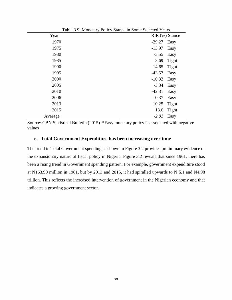
xx
Table 3.9: Monetary Policy Stance in Some Selected Years
Year RIR (%) Stance
1970 -29.27 Easy
1975 -13.97 Easy
1980 -3.55 Easy
1985 3.69 Tight
1990 14.65 Tight
1995 -43.57 Easy
2000 -10.32 Easy
2005 -3.34 Easy
2010 -42.31 Easy
2006 -0.37 Easy
2013 10.25 Tight
2015 13.6 Tight
Average -2.01 Easy
Source: CBN Statistical Bulletin (2015). *Easy monetary policy is associated with negative
values
e. Total Government Expenditure has been increasing over time
The trend in Total Government spending as shown in Figure 3.2 provides preliminary evidence of
the expansionary nature of fiscal policy in Nigeria. Figure 3.2 reveals that since 1961, there has
been a rising trend in Government spending pattern. For example, government expenditure stood
at N163.90 million in 1961, but by 2013 and 2015, it had spiralled upwards to N 5.1 and N4.98
trillion. This reflects the increased intervention of government in the Nigerian economy and that
indicates a growing government sector.

xxi
Figure 3.2: Trend in Total Government Expenditure 1960-2015
Source: CBN Statistical Bulletin (2013, 2015)
In terms of per cent growth, Total Government Expenditure grew from 22.81 per cent in the period
1961-1970 to 38.25 per cent in the 70s. This upward trend is closely linked to revenue accrued
from the oil boom of the early 1970s. In the period from 1981 to 1990, government expenditure
declined to 17.68 per cent largely due to the austerity measures in the 80s. By the period 1991-
2000, Total Government Expenditure rebounded to 33.95 per cent before it reduced to 14.82 per
cent over the period of 2000-2015, as shown in Table 3.10. The pattern of growth in the total
Government Expenditure across the various decades, especially in the 70s and 80s, mirrors the
procyclical nature of fiscal policy in Nigeria. The procyclical stance shows that the direction of
government spending correlates positively with movements in oil prices and thus, oil revenue. This
means that government spending rises with increased oil revenue and falls when the oil revenue
dwindles.
0
1.0
e+
06
2.0
e+
06
3.0
e+
06
4.0
e+
06
5.0
e+
06
Federa
l G
overn
ment
Expenditure
(N
'mill
ion)
1960 1980 2000 2020Year
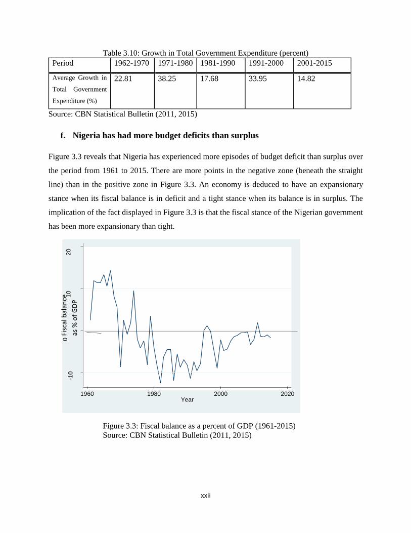
xxii
Table 3.10: Growth in Total Government Expenditure (percent)
Period 1962-1970 1971-1980 1981-1990 1991-2000 2001-2015
Average Growth in
Total Government
Expenditure (%)
22.81 38.25 17.68 33.95 14.82
Source: CBN Statistical Bulletin (2011, 2015)
f. Nigeria has had more budget deficits than surplus
Figure 3.3 reveals that Nigeria has experienced more episodes of budget deficit than surplus over
the period from 1961 to 2015. There are more points in the negative zone (beneath the straight
line) than in the positive zone in Figure 3.3. An economy is deduced to have an expansionary
stance when its fiscal balance is in deficit and a tight stance when its balance is in surplus. The
implication of the fact displayed in Figure 3.3 is that the fiscal stance of the Nigerian government
has been more expansionary than tight.
Figure 3.3: Fiscal balance as a percent of GDP (1961-2015)
Source: CBN Statistical Bulletin (2011, 2015)
-10
0
1
0
20
Fi
scal
bal
ance
as %
of
GD
P
1960 1980 2000 2020 Year
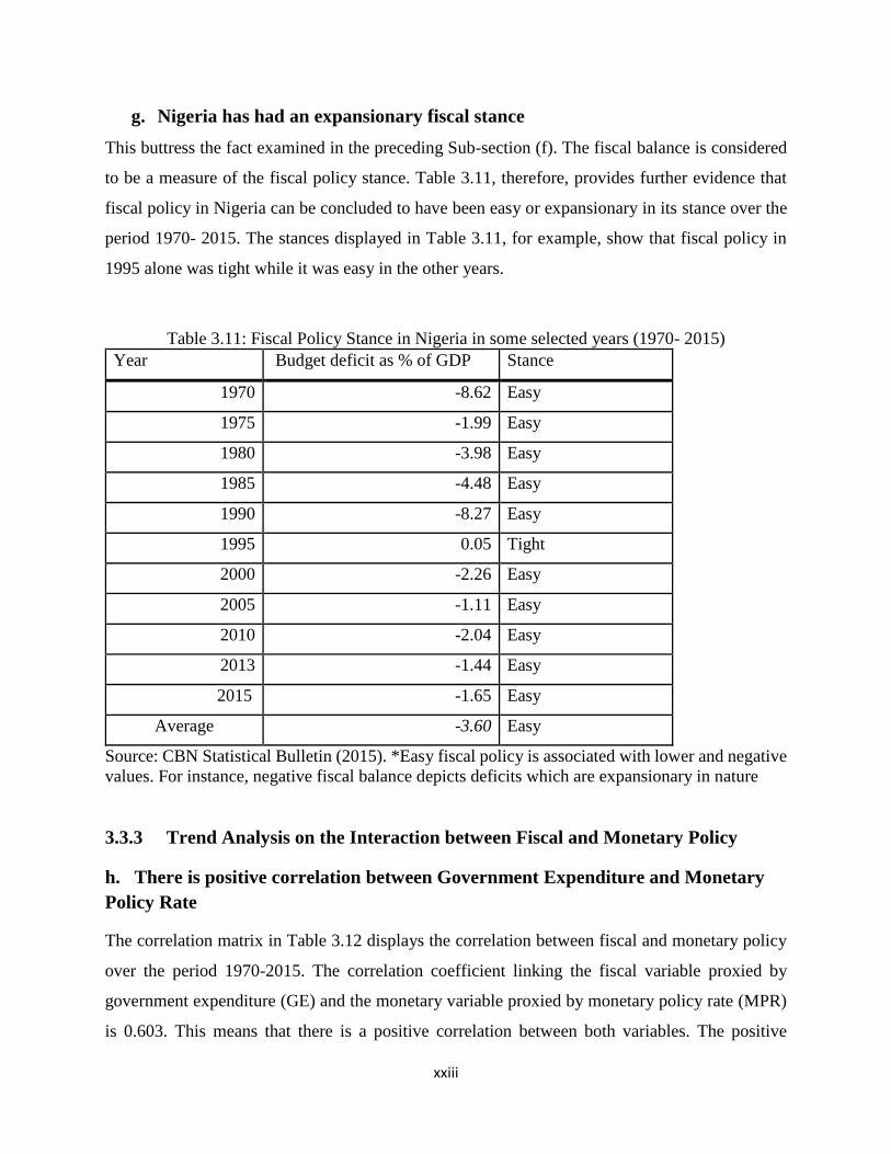
xxiii
g. Nigeria has had an expansionary fiscal stance
This buttress the fact examined in the preceding Sub-section (f). The fiscal balance is considered
to be a measure of the fiscal policy stance. Table 3.11, therefore, provides further evidence that
fiscal policy in Nigeria can be concluded to have been easy or expansionary in its stance over the
period 1970- 2015. The stances displayed in Table 3.11, for example, show that fiscal policy in
1995 alone was tight while it was easy in the other years.
Table 3.11: Fiscal Policy Stance in Nigeria in some selected years (1970- 2015)
Year Budget deficit as % of GDP Stance
1970 -8.62 Easy
1975 -1.99 Easy
1980 -3.98 Easy
1985 -4.48 Easy
1990 -8.27 Easy
1995 0.05 Tight
2000 -2.26 Easy
2005 -1.11 Easy
2010 -2.04 Easy
2013 -1.44 Easy
2015 -1.65 Easy
Average -3.60 Easy
Source: CBN Statistical Bulletin (2015). *Easy fiscal policy is associated with lower and negative
values. For instance, negative fiscal balance depicts deficits which are expansionary in nature
3.3.3 Trend Analysis on the Interaction between Fiscal and Monetary Policy
h. There is positive correlation between Government Expenditure and Monetary
Policy Rate
The correlation matrix in Table 3.12 displays the correlation between fiscal and monetary policy
over the period 1970-2015. The correlation coefficient linking the fiscal variable proxied by
government expenditure (GE) and the monetary variable proxied by monetary policy rate (MPR)
is 0.603. This means that there is a positive correlation between both variables. The positive
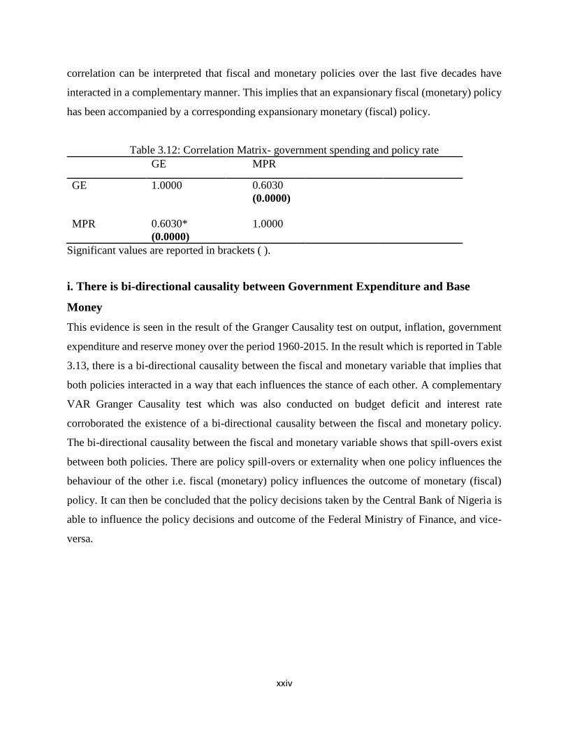
xxiv
correlation can be interpreted that fiscal and monetary policies over the last five decades have
interacted in a complementary manner. This implies that an expansionary fiscal (monetary) policy
has been accompanied by a corresponding expansionary monetary (fiscal) policy.
Table 3.12: Correlation Matrix- government spending and policy rate
GE MPR
GE 1.0000
0.6030
(0.0000)
MPR 0.6030*
(0.0000)
1.0000
Significant values are reported in brackets ( ).
i. There is bi-directional causality between Government Expenditure and Base
Money
This evidence is seen in the result of the Granger Causality test on output, inflation, government
expenditure and reserve money over the period 1960-2015. In the result which is reported in Table
3.13, there is a bi-directional causality between the fiscal and monetary variable that implies that
both policies interacted in a way that each influences the stance of each other. A complementary
VAR Granger Causality test which was also conducted on budget deficit and interest rate
corroborated the existence of a bi-directional causality between the fiscal and monetary policy.
The bi-directional causality between the fiscal and monetary variable shows that spill-overs exist
between both policies. There are policy spill-overs or externality when one policy influences the
behaviour of the other i.e. fiscal (monetary) policy influences the outcome of monetary (fiscal)
policy. It can then be concluded that the policy decisions taken by the Central Bank of Nigeria is
able to influence the policy decisions and outcome of the Federal Ministry of Finance, and vice-
versa.
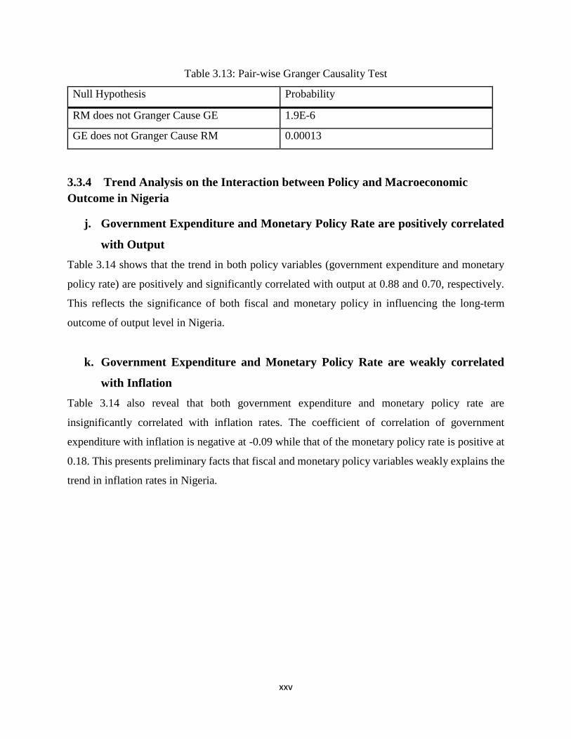
xxv
Table 3.13: Pair-wise Granger Causality Test
Null Hypothesis Probability
RM does not Granger Cause GE 1.9E-6
GE does not Granger Cause RM 0.00013
3.3.4 Trend Analysis on the Interaction between Policy and Macroeconomic
Outcome in Nigeria
j. Government Expenditure and Monetary Policy Rate are positively correlated
with Output
Table 3.14 shows that the trend in both policy variables (government expenditure and monetary
policy rate) are positively and significantly correlated with output at 0.88 and 0.70, respectively.
This reflects the significance of both fiscal and monetary policy in influencing the long-term
outcome of output level in Nigeria.
k. Government Expenditure and Monetary Policy Rate are weakly correlated
with Inflation
Table 3.14 also reveal that both government expenditure and monetary policy rate are
insignificantly correlated with inflation rates. The coefficient of correlation of government
expenditure with inflation is negative at -0.09 while that of the monetary policy rate is positive at
0.18. This presents preliminary facts that fiscal and monetary policy variables weakly explains the
trend in inflation rates in Nigeria.

xxvi
Table 3.14: Correlation Matrix-Policy and Macroeconomic outcomes
GDP INF GE MPR
GDP 1.0000
INF 0.0171
(0.9104)
1.0000
GE 0.8874
(0.0000)
-0.0855
(0.5722)
1.0000
MPR 0.6955
(0.0000)
0.1840
(0.2210)
0.6030*
(0.0000)
1.0000
Significant values are reported in brackets ( ).
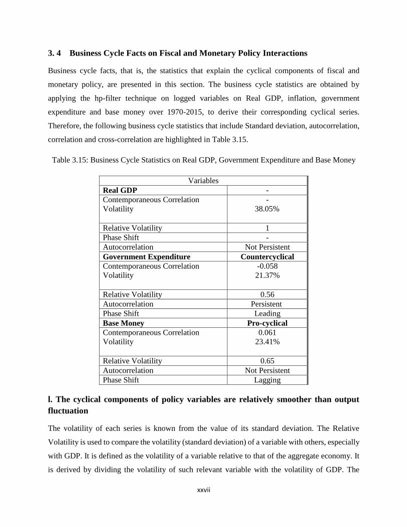
xxvii
3. 4 Business Cycle Facts on Fiscal and Monetary Policy Interactions
Business cycle facts, that is, the statistics that explain the cyclical components of fiscal and
monetary policy, are presented in this section. The business cycle statistics are obtained by
applying the hp-filter technique on logged variables on Real GDP, inflation, government
expenditure and base money over 1970-2015, to derive their corresponding cyclical series.
Therefore, the following business cycle statistics that include Standard deviation, autocorrelation,
correlation and cross-correlation are highlighted in Table 3.15.
Table 3.15: Business Cycle Statistics on Real GDP, Government Expenditure and Base Money
Variables
Real GDP -
Contemporaneous Correlation
Volatility
-
38.05%
Relative Volatility 1
Phase Shift -
Autocorrelation Not Persistent
Government Expenditure Countercyclical
Contemporaneous Correlation
Volatility
-0.058
21.37%
Relative Volatility 0.56
Autocorrelation Persistent
Phase Shift Leading
Base Money Pro-cyclical
Contemporaneous Correlation
Volatility
0.061
23.41%
Relative Volatility 0.65
Autocorrelation Not Persistent
Phase Shift Lagging
l. The cyclical components of policy variables are relatively smoother than output
fluctuation
The volatility of each series is known from the value of its standard deviation. The Relative
Volatility is used to compare the volatility (standard deviation) of a variable with others, especially
with GDP. It is defined as the volatility of a variable relative to that of the aggregate economy. It
is derived by dividing the volatility of such relevant variable with the volatility of GDP. The

xxviii
coefficients describing the relative volatility in Table 3.15 reveal that the cyclical fluctuations in
government expenditure and reserve money are less volatile when compared to economy wide
fluctuation in real GDP.
m. The cyclical components of fiscal and monetary policy variables are weakly
correlated with output
In Table 3.15, the coefficients of the contemporaneous correlation of fiscal and monetary policy
variables (Xt) are seen to be less than 0.5. This depicts the weak association of fluctuations in
policy variables with output fluctuation. It implies that fiscal and monetary policies are fairly
effective for output stabilisation at the short run frequency in Nigeria. However, it can also be
deduced from Table 3.15, that monetary policy has been more effective than fiscal policy, at output
stabilisation, based on the comparison of the magnitude of their contemporaneous correlation
coefficients (Xt ).
n. Fiscal policy is countercyclical
The negative correlation between fluctuations in a variable with fluctuation in aggregate economic
activity is interpreted as being countercyclical. The contemporaneous correlation between
Government expenditure and GDP in Nigeria, is negative (-0.05), as shown in Table 3.15. This
means that when the economy is in a recession (boom), government spending increases
(decreases). The countercyclical nature of government spending in the short run differs from its
procyclical stance over the long run (see section 3.3.4). One caveat to this preliminary fact is that
the correlation coefficient is so close to zero (0) such that countercyclical relationship between
government spending and the state of economy is trivial.
o. Monetary policy is pro-cyclical
The positive correlation of fluctuations in a variable with fluctuations in aggregate economic
activity is interpreted as pro-cyclicality. Base money is shown to be positively correlated with
GDP in Table 3.15. This implies that when the Nigerian economy slides into a recession (boom),
the Central Bank of Nigeria usually responds with a tight (easy) monetary policy. The pro-cyclical
stance of monetary policy at business cycle frequency is similar to the stance found at the long run
frequency (see section 3.3.4).

xxix
p. The cyclical components of fiscal and monetary policy variables are fairly
correlated with price level
The magnitude of the contemporaneous correlation of the cyclical component of government
expenditure and base money with price level is greater when compared to their correlation with
output fluctuations. In Table 3.16, the coefficient of correlation for government expenditure and
base money is 0.2013 and 0.5111 as compared with those presented in Table 3.15 (0.061 and -
0.058). This implies that fiscal and monetary policy tools are more effective at price level
stabilisation than at output stabilisation.
Table 3.16: correlation with CPI
Cyclical components Correlation with CPI
Consumer Price Inflation 1
Government Expenditure 0.2013
(0.1798)
Base Money 0.5111
(0.0003)
Significant values are reported in brackets ( ).
q. Fiscal variable and monetary variables are positively correlated
Table 3.17 shows the positive association between government expenditure and base money; and
between budget deficit and real interest rate. This correlation implies that fiscal and monetary
policies act as complement at business cycle frequency. This means an expansionary fiscal
(monetary) policy is being accompanied by a corresponding expansionary monetary (fiscal) policy
and vice-versa. The positive correlation at business cycle frequency also corresponds with the
result found for the long run frequency (section 3.4.3).

xxx
Table 3.17: Cyclical Correlation between Fiscal and monetary policy
Base Money Government
Expenditure
Government Expenditure
Base Money
0.5600*
(0.0001)
1
1
0.5600
(0.0001)
Significant values are reported in brackets ( ).
3.5 Empirical Facts on Alternative Assumptions
In this section, some empirical evidences buttressing the existence of alternative assumptions,
adopted in this study are presented i.e. rent-seeking, discretionary fiscal policy and weak policy
coordinated. These include:
r. Rent-seeking in Nigeria
According to Martini (2014), there is existing evidence that shows that throughout Nigeria’s post-
colonial history, politicians, members of government and public officials have abused their
positions to extract state resources. This act has taken place through embezzlement of public funds,
nepotism, cronyism, etc.
This evidence is corroborated by the low performance of Nigeria in indices such as Transparency
International’s Corruption Perception Index and the World Governance Indicators. The Corruption
Perception Index is presented in Table 3.18. Table 3.18 shows that between the period 2012 and
2016, Nigeria scored poorly between 25 and 28 out of 100. It indicates that there is deep
corruption/rent-seeking in the country’s public sector. An implication of this index is that with
deep-seated corruption, especially in the public sector, resources are highly likely to be channelled
away for the development of the country, into personal use.
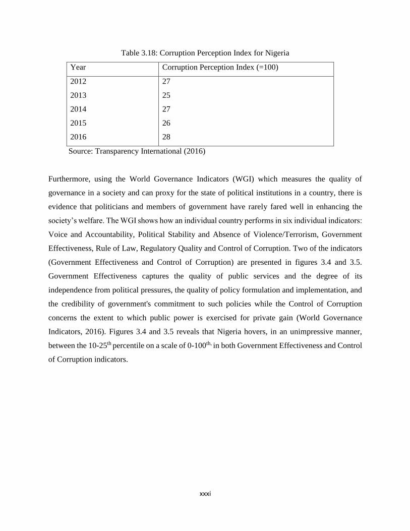
xxxi
Table 3.18: Corruption Perception Index for Nigeria
Year Corruption Perception Index (=100)
2012
2013
2014
2015
2016
27
25
27
26
28
Source: Transparency International (2016)
Furthermore, using the World Governance Indicators (WGI) which measures the quality of
governance in a society and can proxy for the state of political institutions in a country, there is
evidence that politicians and members of government have rarely fared well in enhancing the
society’s welfare. The WGI shows how an individual country performs in six individual indicators:
Voice and Accountability, Political Stability and Absence of Violence/Terrorism, Government
Effectiveness, Rule of Law, Regulatory Quality and Control of Corruption. Two of the indicators
(Government Effectiveness and Control of Corruption) are presented in figures 3.4 and 3.5.
Government Effectiveness captures the quality of public services and the degree of its
independence from political pressures, the quality of policy formulation and implementation, and
the credibility of government's commitment to such policies while the Control of Corruption
concerns the extent to which public power is exercised for private gain (World Governance
Indicators, 2016). Figures 3.4 and 3.5 reveals that Nigeria hovers, in an unimpressive manner,
between the 10-25th percentile on a scale of 0-100th, in both Government Effectiveness and Control
of Corruption indicators.

xxxii
Figure 3.4: Aggregate Indicator on Government Effectiveness in Nigeria over the period 1996-
2015.
Source: World Bank’s World Governance Indicator, 2016
Figure 3.5: Aggregate Indicator on Control of Corruption in Nigeria over the period 1996-2015.
Source: World Bank’s World Governance Indicator, 2016
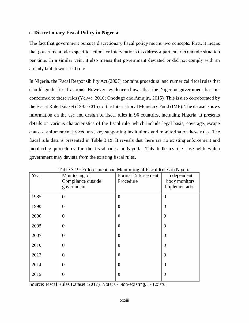
xxxiii
s. Discretionary Fiscal Policy in Nigeria
The fact that government pursues discretionary fiscal policy means two concepts. First, it means
that government takes specific actions or interventions to address a particular economic situation
per time. In a similar vein, it also means that government deviated or did not comply with an
already laid down fiscal rule.
In Nigeria, the Fiscal Responsibility Act (2007) contains procedural and numerical fiscal rules that
should guide fiscal actions. However, evidence shows that the Nigerian government has not
conformed to these rules (Yelwa, 2010; Onodugo and Amujiri, 2015). This is also corroborated by
the Fiscal Rule Dataset (1985-2015) of the International Monetary Fund (IMF). The dataset shows
information on the use and design of fiscal rules in 96 countries, including Nigeria. It presents
details on various characteristics of the fiscal rule, which include legal basis, coverage, escape
clauses, enforcement procedures, key supporting institutions and monitoring of these rules. The
fiscal rule data is presented in Table 3.19. It reveals that there are no existing enforcement and
monitoring procedures for the fiscal rules in Nigeria. This indicates the ease with which
government may deviate from the existing fiscal rules.
Table 3.19: Enforcement and Monitoring of Fiscal Rules in Nigeria
Year Monitoring of
Compliance outside
government
Formal Enforcement
Procedure
Independent
body monitors
implementation
1985
1990
2000
2005
2007
2010
2013
2014
2015
0
0
0
0
0
0
0
0
0
0
0
0
0
0
0
0
0
0
0
0
0
0
0
0
0
0
0
Source: Fiscal Rules Dataset (2017). Note: 0- Non-existing, 1- Exists
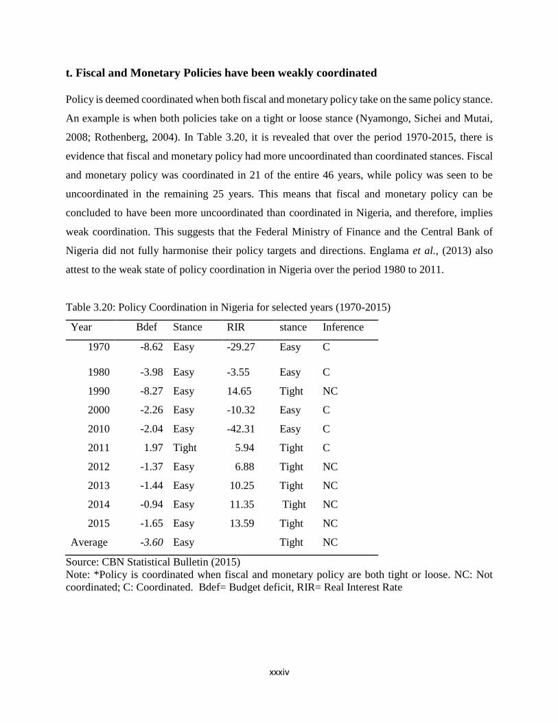
xxxiv
t. Fiscal and Monetary Policies have been weakly coordinated
Policy is deemed coordinated when both fiscal and monetary policy take on the same policy stance.
An example is when both policies take on a tight or loose stance (Nyamongo, Sichei and Mutai,
2008; Rothenberg, 2004). In Table 3.20, it is revealed that over the period 1970-2015, there is
evidence that fiscal and monetary policy had more uncoordinated than coordinated stances. Fiscal
and monetary policy was coordinated in 21 of the entire 46 years, while policy was seen to be
uncoordinated in the remaining 25 years. This means that fiscal and monetary policy can be
concluded to have been more uncoordinated than coordinated in Nigeria, and therefore, implies
weak coordination. This suggests that the Federal Ministry of Finance and the Central Bank of
Nigeria did not fully harmonise their policy targets and directions. Englama et al., (2013) also
attest to the weak state of policy coordination in Nigeria over the period 1980 to 2011.
Table 3.20: Policy Coordination in Nigeria for selected years (1970-2015)
Year Bdef Stance RIR stance Inference
1970 -8.62
Easy -29.27 Easy C
1980 -3.98 Easy -3.55 Easy C
1990 -8.27 Easy 14.65 Tight NC
2000 -2.26 Easy -10.32 Easy C
2010 -2.04 Easy -42.31 Easy C
2011 1.97 Tight 5.94 Tight C
2012 -1.37 Easy 6.88 Tight NC
2013 -1.44 Easy 10.25 Tight NC
2014 -0.94 Easy 11.35 Tight NC
2015 -1.65 Easy 13.59 Tight NC
Average -3.60 Easy Tight NC
Source: CBN Statistical Bulletin (2015)
Note: *Policy is coordinated when fiscal and monetary policy are both tight or loose. NC: Not
coordinated; C: Coordinated. Bdef= Budget deficit, RIR= Real Interest Rate
xxxv
3.6 Summary of Key Issues
Preliminary statistical facts describing fiscal-monetary policy interactions and alternative fiscal
assumptions have been presented in this chapter. The major issues arising from these facts show
that there is preliminary evidence of: (1) positive correlation, that is, complementary interactions
between fiscal and monetary policies in Nigeria (2) bi-directional causality between both policies
such that there is proof of ongoing interactions between fiscal and monetary policies. This means
that fiscal (monetary) policy influences the stance and overall macroeconomic effect of monetary
(fiscal) policy (3) positive and significant impact of both macroeconomic policies on output but
an insignificant influence on the price level (4) the existence of rent-seeking, discretionary fiscal
policy making and weak policy coordination. The aforementioned statistical facts are used as basis
to hypothesise and construct the theoretical model in the next chapter.

xxxvi
CHAPTER FOUR
METHODOLOGY
The theoretical base of this study and the estimation strategy to address its primary objectives are
outlined in this chapter. The Chapter has been divided into three Sections. Section 4.1 discusses
the theoretical framework used in this thesis. In particular, the framework of the New Keynesian
Dynamic Stochastic General Equilibrium model was outlined. Section 4.2 presents the relevant
research method. The Section comprises the model specification and then the applicable estimation
strategy is stated. Thereafter, the data sources and measurement are listed. In Section 4.3, the
method to compute optimal fiscal and monetary policy is examined.
4.1 Theoretical Framework
The theoretical base of this work hinges on the New Keynesian School of economic thought. The
model is first presented and then, applied in the context of this study.
4.1.1 The New Keynesian Macro-Economic Model
The New Keynesian model is the theoretical underpinning of this study. This school of economic
thought sprang up in the 1980s after the New Classicals such as Robert Lucas and Thomas Sargent
critiqued some existing traditional Keynesian ideas. For example, the Keynesians developed and
estimated large scale macro econometric models that could be used to predict and forecast the
impact of policy. Critics like Robert Lucas believed that the specified model lacked a theoretical
foundation and that estimated parameters in such models will vary in response to changes in policy
intervention. This variation implies that policy recommendation is time-inconsistent and is
regarded as a potential drawback to policy analysis and forecast. Lucas argued for the formulation
of structural econometric models with a strong theoretical underpinning and micro foundation that
captures an economy’s structure. This requires developing models that captures the forward-
xxxvii
looking and optimising behaviour of economic agents in macroeconomic models to be used for
policy analysis.
The work of Mankiw and Romer (1991) is regarded as one of the major contributions to the New
Keynesian School. This school maintains traditional Keynesian ideas that include the existence of
imperfect competition among firms and the notion of sticky prices and wages. The implications of
these assumptions are that there are frictions that prevent prices and wages from adjusting quickly
to shocks and market failures are possible. This necessitates the intervention of government
through stabilisation policies to adjust the price mechanism and return the economy to equilibrium.
The Keynesian also advise the use of stabilisation policies because monetary policy has non-
neutral effects on the economy.
Based on the Lucas critique, the New Keynesian School adopts the micro foundation of the Real
Business cycle (RBC) model as expounded by the New Classical, in explaining the existing
macroeconomic theories of the traditional Keynesians. They also borrow from the rational
expectation school which assume forward looking households and firms who make decisions
based on the expectation of the future. This culminates in a methodological framework introduced
by the New Classical: the dynamic general equilibrium method (DGE).
The New Keynesian Dynamic General Equilibrium Models recognise the forward looking and
optimising behaviour of economic agent. They deviate from traditional assumptions of frictionless
markets, flexible prices and neutrality of money. They recognise the existence of real and nominal
shocks, non-trivial effect of monetary policy, monopolistic competition and nominal rigidity. In
the canonical model, there are 3 economic agents: the household, firms and central banks. The
household purchases goods, holds money and bonds, supplies labour to the firms and maximises
its expected present value of utility. There are two types of firms: intermediate and final goods
producers. The firms produce differentiated products in monopolistic competition while the
Central Bank sets the nominal interest rate using Taylor-type rules.
The New Keynesian Dynamic Stochastic General Equilibrium (DSGE) model has been adopted
for this study and is most appropriate to examine fiscal and monetary policy interactions since it
is regarded as a workhorse for macroeconomic policy analysis and has been used by central banks

xxxviii
around the world for such purpose. Secondly, the model recognises a role for fiscal and monetary
policy in stabilising the economy in the face of shocks. Thirdly, the DSGE model provides a natural
setting to examine policy interactions since it assumes existing interdependencies among economic
agents in the different sectors.
The Standard New Keynesian DSGE Model
The NK DSGE models stem from the contributions of scholars such as Gali and Gertler (1999),
Smets and Wouters (2003, 2007), Gali (2003), Christiano, Eichenbaum and Evans (2005). In these
models, there are three optimising agents: households, firms and the Central Bank. The abridged
model (detailed model is found in sub-section 4.2.1) entails:
Household: A representative household derives utility from consumption and disutility from
labour, and maximises his utility function:
Max1
0
0 1
t itit
t
CE L
(4.1)
Where 𝐸0: Rational expectation operator
𝛽𝑡: intertemporal discount factor
𝛾: Inverse of elasticity of substitution
𝐶𝑡: Consumption
𝐿𝑡: Amount of labour supplied
subject to the inter-temporal household budget constraint (equation 4.2) which shows the total
income versus their total outlay and is specified as:
𝑃𝑡𝐶𝑡 + 𝐸𝑡(𝑄𝑡 ,𝑡+1𝐷𝑡+1) ≤ 𝑊𝑡𝑁𝑡 + 𝐷𝑡 + 𝑇𝑃𝑡 + 𝐷𝑉𝑡 (4.2)
Where,
𝑊𝑡𝑁𝑡: Wage bill
𝑇𝑃𝑡: Transfer payment from government
𝐷𝑉𝑡: Dividend
𝑟𝑡: Nominal interest rate

xxxix
𝐷𝑡+1: Payment at period 𝑡 + 1 from a portfolio of state contingent claims
𝐸𝑡(𝑄𝑡 ,𝑡+1): One period ahead stochastic discount factor
Aggregate resource constraint: It is assumed that there is no capital in the economy. Total sum
of consumption (𝐶𝑡) at each period t of all individual (𝐶𝑖𝑡), therefore, equals the total sum of income
(𝑌𝑖𝑡) of all individuals in the economy and it is given as follows:
1 1
I I
t it it
i i
C C Y
(4.3)
Firms: The firms produce the goods and services in the economy (𝑌𝑖𝑡) with a linear production
function using labour inputs (𝐿𝑖𝑡) and technology (𝑧𝑡) such that:
it t itY z L
(4.4)
The firms are also faced with a price setting decision. They follow the Calvo (1983) staggered
price-setting mechanism such that while a fraction 𝜇 cannot reset their prices, the other fraction
1 − 𝜇 can. Therefore, in order to fix prices, 𝑃𝐷,𝑡∗ , the firms must reset their prices by maximising
their real discounted profits subject to demand such that:
Max Et ∑ (βθ)k∞k=0 Et,t+k Yt+k(i) [𝑃𝐷,𝑡
∗ − mct+k] (4.5)
Subject to
𝑌t+k(i) = [𝑃𝐷,𝑡
∗
𝑃𝑡+𝑘]
−𝜀
𝑌𝑡+𝑘 (4.6)
Where,
Et,t+k : Stochastic discount factor for nominal payoffs in period t + k
Yt+k(i) : Output in period t + k of good i
𝑃𝐷,𝑡∗ : Fixed price that maximises real discounted profits
mct+k: Real marginal cost in period t + k
Et : Rational Expectation Operator
Βθ: Probability that firms reset prices

xl
Central Bank: The Central Bank set nominal interest rate by following a Taylor type rule where
the interest rate responds to the inflation rate and output growth
Rt
R= [
Rt−1
R]
ρR
[(πt
π)
φπ
(Yt
Y)
φY
(St
S)
φS
]1−ρR
εtR (4.7)
Where,
Rt: Interest rate
Rt−1: lagged interest rate
πt: Inflation rate
Yt: Output growth
St: Exchange rate
εtR: Innovation to monetary policy
ρR: Degree of interest rate smoothing
φπ, φY, φS: Parameters that measures the response of Central Bank to inflation, output and
exchange rate. In addition, R, π, Y, S are the target values of interest rate, inflation rate, output
and exchange rate.
Exogenous Stochastic processes: It is assumed that both real and nominal shocks perturb the
economy. The shocks are modelled as autoregressive processes of lagged innovations of order one,
as defined in equation (4.8):
1t t tz z
(4.8)
휀𝑡~ 𝑖. 𝑖. 𝑑 (0, 𝜎𝜀)
The preceding canonical model omits the fiscal sector. The model has therefore been extended to
include the fiscal sector. The New Keynesian DSGE models with fiscal policy initially assumed
the existence of Ricardian equivalence i.e: a passive or neutral role for fiscal policy. In these
models there is lump sum taxation and the government faces an inter-temporal solvency condition
(Leeper, 1991; Leeper and Leith, 2015; Sims, 1994; Bianchi and Ilut, 2016). A later variant of the
New Keynesian DSGE model gives an explicit role to fiscal policy which sets a policy rule and
introduces non-Ricardian fiscal effects by assuming the existence of rule of thumb households.
The inclusion of rule of thumb agents engenders the non-neutral effect of fiscal policy on the
xli
economy (Gali, Lopez-Salido, and Valles, 2007; Algozhina, 2012; Rossi, 2014). This study will
include these recent features to capture the interaction between fiscal and monetary policy.
In conclusion, some of the reasons for adopting the New Keynesian model include its usefulness
for policy analysis since it identifies a role for stabilising (fiscal and monetary) policies. It
recognises the importance of both real and nominal shocks. It also utilizes a rich dynamic
optimising and microeconomic background for analysing the decisions of economic agents. It
recognises the existence of frictions, nominal rigidities and imperfect markets that underlie the
dual structure of developing economies such as Nigeria. At the same time, with the apparent
disequilibrium between aggregate demand and supply in the Nigerian economy, this study has
adopted the NK model (Alege, 2008). The model can also be estimated and provides good policy
forecast and evaluation.
4.2 The Research Method
This thesis argues that the fiscal decision of government interacts with instruments and targets of
monetary policy in Nigeria. This study is, therefore, concerned with empirically testing existing
theoretical propositions for the impact that fiscal policy wields on monetary outcomes in Nigeria
and vice-versa. It also examines the effect of the policy interactions on output and inflation in
Nigeria. The study, therefore, investigates fiscal and monetary interactions within an Open
Economy New Keynesian DSGE Model that deviates from the assumptions of a benevolent
government who commits to a policy rule. In this instance, government is assumed to have rent-
seeking tendencies and prefers to use policy discretion in maximising the welfare of a subset of
the society (see sub-section 3.5 to prove the relevance of rent-seeking and policy discretion in
Nigeria). The adopted assumptions indicate that this study considers the underlying political
dimensions to economic policy.
This study captures the rent-seeking tendencies of the fiscal bloc by specifying a utility function
which shows that the government benefits from both providing public goods and from rent-seeking
activities that boosts its personal gains. The utility function also admits a fiscal shock and a
parameter on the quality of existing political institution, which serves in a complementary manner
as another proxy to capture the rent-seeking ability of the government (see equations 4.89 - 4.99
xlii
in sub-section 4.2.1). In addition, the discretionary policy of government is illustrated in this study
by considering the micro-foundation of the fiscal sector, in contrast to specifying a fiscal (Taylor-
type) rule. The government is assumed in this instance, to maximise its per period utility function
subject to its budget constraint (Fragetta and Kirsanova, 2010).
4.2.1 An Open Economy New Keynesian DSGE Model for Nigeria
(a) Structure of the Model
The model is constructed drawing on the works of Gali and Monacelli (2005), Gali and Monacelli
(2008), Gali (2008), Almeida (2010), Senbeta (2011), Rossi (2014), Miller (2016), Li and Spencer
(2014) and Adegboye (2015). The study adapted the political economy assumption from Miller
(2016). The remaining studies aforementioned were instrumental in constructing the Small Open
Economy (SOE) NK DSGE model. The DSGE model adopted in this study comprises of five
optimising agents: households, firms, the central bank, government and rest of the world, who
form model-consistent expectation based on available information. The infinitely lived household
decides how much units of goods to consume and labour to supply in order to maximise its lifetime
utility subject to budget constraints. It is assumed that there are two types of household, the
Ricardian and Non-Ricardian. Unlike the Ricardian, the Non-Ricardian agent is liquidity-
constrained and lacks access to the financial market (Conen and Straub, 2005; Gali, Lopez-Salido
and Valles, 2007 as cited in Torres, 2015). A large amount of Non- Ricardian consumers implies
that fiscal policy is not passive as proposed in models with Ricardian equivalence (Rossi, 2014).
The household also form habits in their consumption. This means that utility is time non-separable;
it depends on consumption in previous period. The household sector is also assumed to supply
labour to firms in a perfectly competitive labour market.
In the production sector, there are the final-good producer and the intermediate-goods producers.
The final-good producer operates under a perfectly-competitive market and can re-optimise their
prices. The final-good producer aggregates the goods of the intermediate firms using the Dixit-
Stiglitz (1977) framework. The intermediate-goods producers are in monopolistic competition and
cannot change prices. Following the Calvo (1983) sticky price setting, a fraction of the
intermediate-goods firms is allowed to re-set their price. The third agent is a monetary authority,
xliii
the Central Bank of Nigeria that implements monetary policy by following a Taylor-type rule to
set its policy rate. It is also posited that Nigeria is a small open economy linked to a foreign
economy, which is the Rest of the World. As a small open economy, the size of the Nigerian
economy is tiny and lacks a significant influence on the Rest of the World. Finally, there are some
exogenous shock processes.
The fiscal authority, the Federal Government of Nigeria, is the fifth agent. In many instances, the
fiscal authority is modelled to be benevolent i.e. it is concerned with the welfare of the whole
society (Algozhina, 2012; Leeper and Leith, 2015; Bianchi and Ilut, 2016). It purchases from firms,
issue bonds, collects lump sum taxes, and makes transfer payment to keep balanced budget.
Secondly, in these studies, the government commits to a fiscal rule in spending and taxes. This
present study deviates from these two assumptions, since they may not be realistic in developing
economies such as Nigeria.
The study rather assumes the existence of political friction i.e. the government may be concerned
with maximising the benefit of a subset of its citizen due to its rent-seeking tendencies (Miller,
2016). Secondly, it is postulated that the fiscal authority uses discretion in choosing its policy on
spending and taxes. An implication is that, if the monetary authority commits to a rule while the
fiscal authority relies on discretion, this can be termed a non-cooperative policy game, further
implying weak or non-existing coordination between the two policies (Dixit and Lambertini,
2003). This conjecture is realistic since there is evidence of weak coordination between fiscal and
monetary policy in Nigeria (Englama et al., 2013). The model adopted for this study, therefore, is
a Small Open Economy, Dynamic Stochastic General Equilibrium model which comprises of two
types of households, firms, the monetary authority and a rent-seeking, discretionary fiscal bloc.
(b) The Model
In what follows, the study presents the relevant equations of the Small Open Economy, Dynamic
Stochastic General Equilibrium model. Each sector is considered in order to derive its optimisation
conditions.
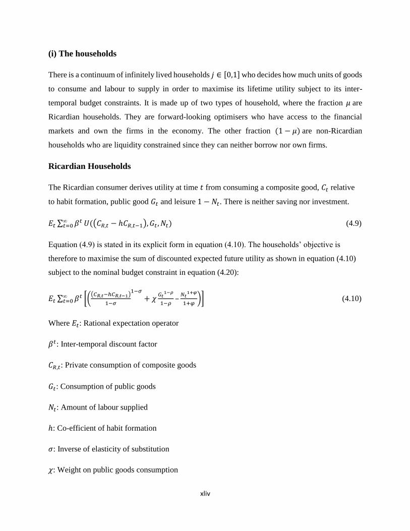
xliv
(i) The households
There is a continuum of infinitely lived households 𝑗 ∈ [0,1] who decides how much units of goods
to consume and labour to supply in order to maximise its lifetime utility subject to its inter-
temporal budget constraints. It is made up of two types of household, where the fraction 𝜇 are
Ricardian households. They are forward-looking optimisers who have access to the financial
markets and own the firms in the economy. The other fraction (1 − 𝜇) are non-Ricardian
households who are liquidity constrained since they can neither borrow nor own firms.
Ricardian Households
The Ricardian consumer derives utility at time 𝑡 from consuming a composite good, 𝐶𝑡 relative
to habit formation, public good 𝐺𝑡 and leisure 1 − 𝑁𝑡. There is neither saving nor investment.
𝐸𝑡 ∑ 𝛽𝑡∞𝑡=0 𝑈((𝐶𝑅,𝑡 − ℎ𝐶𝑅,𝑡−1), 𝐺𝑡 , 𝑁𝑡) (4.9)
Equation (4.9) is stated in its explicit form in equation (4.10). The households’ objective is
therefore to maximise the sum of discounted expected future utility as shown in equation (4.10)
subject to the nominal budget constraint in equation (4.20):
𝐸𝑡 ∑ 𝛽𝑡∞𝑡=0 [(
(𝐶𝑅,𝑡−ℎ𝐶𝑅,𝑡−1)
1−𝜎
1−𝜎
+ 𝜒𝐺𝑡
1−𝜌
1−𝜌–
𝑁𝑡1+𝜑
1+𝜑)] (4.10)
Where 𝐸𝑡: Rational expectation operator
𝛽𝑡: Inter-temporal discount factor
𝐶𝑅,𝑡: Private consumption of composite goods
𝐺𝑡: Consumption of public goods
𝑁𝑡: Amount of labour supplied
ℎ: Co-efficient of habit formation
𝜎: Inverse of elasticity of substitution
𝜒: Weight on public goods consumption

xlv
𝜑: Inverse on Frisch elasticity of labour supply
ℎ, 𝜎, 𝜒, 𝜑 > 0; 0 < 𝛽𝑡 < 1
Consumption,𝐶𝑅,𝑡, is a composite good which consists of domestic goods 𝐶𝐷,𝑡 and foreign goods
𝐶𝐹,𝑡. This implies that the household allocates its resources in consuming both domestically
produced goods and imported goods. The composite good 𝐶𝑅,𝑡 is defined using the Dixit-Stiglitz
(1977) Constant Elasticity of Substitution in equation (4.11)
𝐶𝑅,𝑡 ≡ [(1 − 𝛼)1
𝜂𝐶𝐷,𝑡
𝜂−1
𝜂 + (𝛼)1
𝜂𝐶𝐹,𝑡
𝜂−1
𝜂 ]
𝜂
𝜂−1
(4.11)
Where 𝐶𝐷,𝑡: Index of consumption of domestic goods
𝐶𝐹,𝑡: Index of consumption of foreign goods
1 − 𝛼: Degree of openness
𝛼: Home-bias parameter
휂: Elasticity of substitution between domestic and foreign goods
And where 𝐶𝐷,𝑡 and 𝐶𝐹,𝑡 are assumed to be Dixit-Stiglitz (1977) aggregators of individual
consumption goods. They comprise of a continuum of both domestic and foreign goods given by:
𝐶𝐷,𝑡 = [∫ 𝐶𝐷,𝑡 (𝑖)𝜀−1
𝜀 𝑑𝑖]
𝜀
𝜀−1 (4.12)
𝐶𝐹,𝑡 = [∫ 𝐶𝐹,𝑡 (𝑖)𝜀−1
𝜀 𝑑𝑖]
𝜀
𝜀−1 (4.13)
In equations (4.12) and (4.13), parameter 휀 > 1 is the elasticity of substitution between different
goods produced in the domestic economy.
The household decides to allocate a given level of expenditure between domestic and foreign
goods. They minimise total expenditure on domestic and foreign goods in equation (4.14)
Min 𝑃𝑡𝐶𝑅,𝑡 = 𝑃𝐷,𝑡𝐶𝐷,𝑡 + 𝑃𝐹,𝑡𝐶𝐹,𝑡 (4.14)
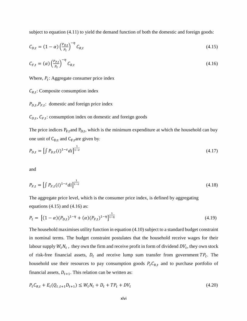
xlvi
subject to equation (4.11) to yield the demand function of both the domestic and foreign goods:
𝐶𝐷,𝑡 = (1 − 𝛼) (𝑃𝐷,𝑡
𝑃𝑡)
−𝜂
𝐶𝑅,𝑡 (4.15)
𝐶𝐹,𝑡 = (𝛼) (𝑃𝐹,𝑡
𝑃𝑡)
−𝜂
𝐶𝑅,𝑡 (4.16)
Where, 𝑃𝑡: Aggregate consumer price index
𝐶𝑅,𝑡: Composite consumption index
𝑃𝐷,𝑡,𝑃𝐹,𝑡: domestic and foreign price index
𝐶𝐷,𝑡, 𝐶𝐹,𝑡: consumption index on domestic and foreign goods
The price indices PF,tand PD,t, which is the minimum expenditure at which the household can buy
one unit of CD,t and CF,tare given by:
𝑃𝐷,𝑡 = [∫ 𝑃𝐷,𝑡(𝑖)1−𝜀𝑑𝑖]1
1−𝜀 (4.17)
and
𝑃𝐹,𝑡 = [∫ 𝑃𝐹,𝑡(𝑖)1−𝜀𝑑𝑖]1
1−𝜀 (4.18)
The aggregate price level, which is the consumer price index, is defined by aggregating
equations (4.15) and (4.16) as:
𝑃𝑡 = [(1 − 𝛼)(𝑃𝐷,𝑡)1−𝜂 + (𝛼)(𝑃𝐹,𝑡)1−𝜂]1
1−𝜂 (4.19)
The household maximises utility function in equation (4.10) subject to a standard budget constraint
in nominal terms. The budget constraint postulates that the household receive wages for their
labour supply 𝑊𝑡𝑁𝑡 , they own the firm and receive profit in form of dividend 𝐷𝑉𝑡, they own stock
of risk-free financial assets, 𝐷𝑡 and receive lump sum transfer from government 𝑇𝑃𝑡. The
household use their resources to pay consumption goods 𝑃𝑡𝐶𝑅,𝑡 and to purchase portfolio of
financial assets, 𝐷𝑡+1. This relation can be written as:
𝑃𝑡𝐶𝑅,𝑡 + 𝐸𝑡(𝑄𝑡 ,𝑡+1𝐷𝑡+1) ≤ 𝑊𝑡𝑁𝑡 + 𝐷𝑡 + 𝑇𝑃𝑡 + 𝐷𝑉𝑡 (4.20)
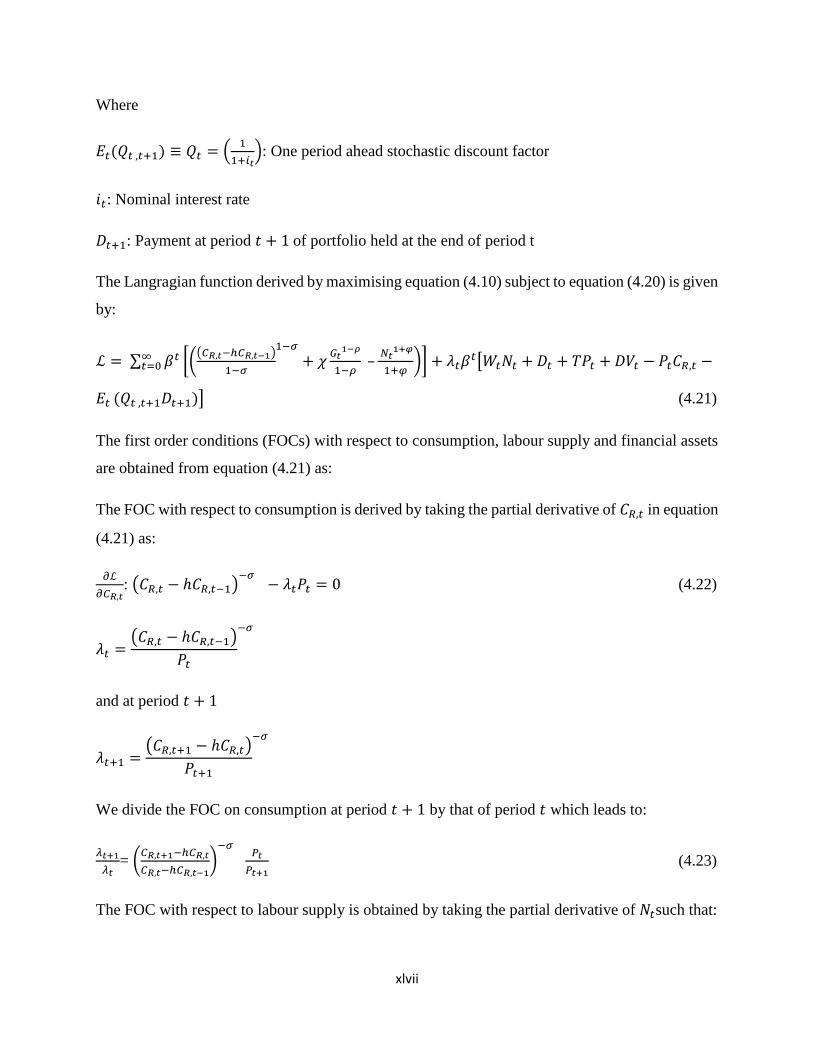
xlvii
Where
𝐸𝑡(𝑄𝑡 ,𝑡+1) ≡ 𝑄𝑡 = (1
1+𝑖𝑡): One period ahead stochastic discount factor
𝑖𝑡: Nominal interest rate
𝐷𝑡+1: Payment at period 𝑡 + 1 of portfolio held at the end of period t
The Langragian function derived by maximising equation (4.10) subject to equation (4.20) is given
by:
ℒ = ∑ 𝛽𝑡∞𝑡=0 [(
(𝐶𝑅,𝑡−ℎ𝐶𝑅,𝑡−1)
1−𝜎
1−𝜎
+ 𝜒𝐺𝑡
1−𝜌
1−𝜌 –
𝑁𝑡1+𝜑
1+𝜑)] + 𝜆𝑡𝛽𝑡[𝑊𝑡𝑁𝑡 + 𝐷𝑡 + 𝑇𝑃𝑡 + 𝐷𝑉𝑡 − 𝑃𝑡𝐶𝑅,𝑡 −
𝐸𝑡 (𝑄𝑡 ,𝑡+1𝐷𝑡+1)] (4.21)
The first order conditions (FOCs) with respect to consumption, labour supply and financial assets
are obtained from equation (4.21) as:
The FOC with respect to consumption is derived by taking the partial derivative of 𝐶𝑅,𝑡 in equation
(4.21) as:
𝜕ℒ
𝜕𝐶𝑅,𝑡: (𝐶𝑅,𝑡 − ℎ𝐶𝑅,𝑡−1)
−𝜎− 𝜆𝑡𝑃𝑡 = 0 (4.22)
𝜆𝑡 =(𝐶𝑅,𝑡 − ℎ𝐶𝑅,𝑡−1)
𝑃𝑡
−𝜎
and at period 𝑡 + 1
𝜆𝑡+1 =(𝐶𝑅,𝑡+1 − ℎ𝐶𝑅,𝑡)
𝑃𝑡+1
−𝜎
We divide the FOC on consumption at period 𝑡 + 1 by that of period 𝑡 which leads to:
𝜆𝑡+1
𝜆𝑡= (
𝐶𝑅,𝑡+1−ℎ𝐶𝑅,𝑡
𝐶𝑅,𝑡−ℎ𝐶𝑅,𝑡−1)
−𝜎𝑃𝑡
𝑃𝑡+1 (4.23)
The FOC with respect to labour supply is obtained by taking the partial derivative of 𝑁𝑡such that:

xlviii
𝜕ℒ
𝜕𝑁𝑡:−𝑁𝑡
𝜑+ 𝜆𝑡𝑊𝑡 = 0 (4.24)
𝜆𝑡 = 𝑁𝑡
𝜑
𝑊𝑡
As usual, the FOC on financial asset is derived by taking the partial derivative of 𝐷𝑡. This yields:
𝑄𝑡 ,𝑡+1 = 𝛽 𝜆𝑡+1
𝜆𝑡 (4.25)
Substitute equation (4.23) into equation (4.25), this becomes:
𝑄𝑡 ,𝑡+1 = 𝛽 (𝐶𝑅,𝑡+1−ℎ𝐶𝑅,𝑡
𝐶𝑅,𝑡−ℎ𝐶𝑅,𝑡−1)
−𝜎𝑃𝑡
𝑃𝑡+1 (4.26)
Take expectations of both sides of equation (4.26). This becomes:
𝐸𝑡𝑄𝑡 ,𝑡+1 = 𝛽𝐸𝑡 [(𝐶𝑅,𝑡+1−ℎ𝐶𝑅,𝑡
𝐶𝑅,𝑡−ℎ𝐶𝑅,𝑡−1)
−𝜎𝑃𝑡
𝑃𝑡+1] (4.27)
Where 𝐸𝑡𝑄𝑡 ,𝑡+1 ≡ 𝑄𝑡 = 1
(𝑅𝑡). This is substituted into equation (4.27) which can then be re-
written as:
1 = 𝛽𝑅𝑡𝐸𝑡 (𝐶𝑅,𝑡+1−ℎ𝐶𝑅,𝑡
𝐶𝑅,𝑡−ℎ𝐶𝑅,𝑡−1)
−𝜎𝑃𝑡
𝑃𝑡+1 (4.28)
Equation (4.28) is the consumption Euler Equation. The inter-temporal consumption Euler
equation is one of the two major optimality conditions for the household sector. It describes the
optimal consumption of the household between the current and future period.
Equation (4.28) is log-linearised to obtain:
𝑐𝑅,𝑡 − ℎ𝑐𝑅,𝑡−1 = 𝐸𝑡(𝑐𝑅,𝑡+1 − ℎ𝑐𝑅,𝑡) −1−ℎ
𝜎(𝑟𝑡 − 𝐸𝑡Π𝑡+1) (4.29)
Where,
Π𝑡+1 = 𝑃𝑡+1 − 𝑃𝑡

xlix
The second optimality condition is the intra-temporal consumption. It shows the marginal rate of
substitution between consumption and labour supply. To derive the intra-temporal consumption
equation, we combine the FOC on consumption with that of labour supply such that:
𝜆𝑡 = 𝑁𝑡
𝜑
𝑊𝑡
and
𝜆𝑡 =(𝐶𝑅,𝑡 − ℎ𝐶𝑅,𝑡−1)
𝑃𝑡
−𝜎
This becomes:
𝑁𝑡𝜑
𝑊𝑡=
(𝐶𝑅,𝑡−ℎ𝐶𝑅,𝑡−1)
(1+𝜏)𝑃𝑡
−𝜎
(4.30)
Equation (4.30) is re-arranged and yields:
𝑊𝑡
𝑃𝑡= (𝐶𝑅,𝑡 − ℎ𝐶𝑅,𝑡−1)
𝜎𝑁𝑡
𝜑(1 + 𝜏) (4.31)
Log-linearise equation (4.31) to get the labour supply schedule for the Ricardian household. This
becomes:
𝑤𝑡 − 𝑝𝑡 =𝜎
1−ℎ(𝑐𝑅,𝑡 − ℎ𝑐𝑅,𝑡−1) + 𝜑𝑛𝑡 (4.32)
Non-Ricardian Household
The liquidity constrained consumer maximises the same utility function in equation (4.10) subject
to the budget constraint in equation (4.33):
𝑃𝑡𝐶𝑁𝑅,𝑡 ≤ 𝑊𝑡𝑁𝑁𝑅,𝑡 + 𝑇𝑃𝑡 (4.33)
The budget constraint postulates that the household receives only wage bills 𝑊𝑡𝑁𝑡 and lump sum
transfer from the government 𝑇𝑃𝑡 and uses its income to buy consumption goods. The budget
constraint takes this form since it is assumed that the non-Ricardian household cannot accumulate
bonds from the financial market and cannot earn profit since they do not own firms.
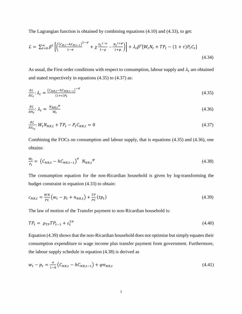
l
The Lagrangian function is obtained by combining equations (4.10) and (4.33), to get:
ℒ = ∑ 𝛽𝑡∞𝑡=0 [(
(𝐶𝑅,𝑡−ℎ𝐶𝑅,𝑡−1)
1−𝜎
1−𝜎
+ 𝜒𝐺𝑡
1−𝜌
1−𝜌 –
𝑁𝑡1+𝜑
1+𝜑)] + 𝜆𝑡𝛽𝑡[𝑊𝑡𝑁𝑡 + 𝑇𝑃𝑡 − (1 + 𝜏)𝑃𝑡𝐶𝑡]
(4.34)
As usual, the First order conditions with respect to consumption, labour supply and 𝜆𝑡 are obtained
and stated respectively in equations (4.35) to (4.37) as:
𝜕ℒ
𝜕𝐶𝑡: 𝜆𝑡 =
(𝐶𝑁𝑅,𝑡−ℎ𝐶𝑁𝑅,𝑡−1)
(1+𝜏)𝑃𝑡
−𝜎
(4.35)
𝜕ℒ
𝜕𝑁𝑡: 𝜆𝑡 =
𝑁𝑁𝑅,𝑡𝜑
𝑊𝑡 (4.36)
𝜕ℒ
𝜕𝜆𝑡𝑡
: 𝑊𝑡𝑁𝑁𝑅,𝑡 + 𝑇𝑃𝑡 − 𝑃𝑡𝐶𝑁𝑅,𝑡 = 0 (4.37)
Combining the FOCs on consumption and labour supply, that is equations (4.35) and (4.36), one
obtains:
𝑊𝑡
𝑃𝑡= (𝐶𝑁𝑅,𝑡 − ℎ𝐶𝑁𝑅,𝑡−1)
𝜎𝑁𝑁𝑅,𝑡
𝜑 (4.38)
The consumption equation for the non-Ricardian household is given by log-transforming the
budget constraint in equation (4.33) to obtain:
𝑐𝑁𝑅,𝑡 =𝑊𝑁
𝑃𝐶(𝑤𝑡 − 𝑝𝑡 + 𝑛𝑁𝑅,𝑡) +
𝑇𝑃
𝑃𝐶(𝑡𝑝𝑡) (4.39)
The law of motion of the Transfer payment to non-Ricardian household is:
𝑇𝑃𝑡 = 𝜌𝑇𝑃𝑇𝑃𝑡−1 + 휀𝑡𝑇𝑃 (4.40)
Equation (4.39) shows that the non-Ricardian household does not optimise but simply equates their
consumption expenditure to wage income plus transfer payment from government. Furthermore,
the labour supply schedule in equation (4.38) is derived as
𝑤𝑡 − 𝑝𝑡 =𝜎
1−ℎ(𝐶𝑁𝑅,𝑡 − ℎ𝐶𝑁𝑅,𝑡−1) + 𝜑𝑛𝑁𝑅,𝑡 (4.41)

li
(ii) The firms
Following Gali and Monacelli (2005), it is assumed that there is a continuum of identical
monopolistic competitive firms 𝑗 ∈ [0,1], in the domestic economy, that produce differentiated
goods using a linear production technology with labour as the only input:
𝑌𝑡(𝑗) = 𝐴𝑡𝑁𝑡(𝑗) (4.42)
Where
𝐴𝑡: Total Factor Productivity
𝑁𝑡(𝑗): Labour input for each firm
Log 𝐴𝑡 ≡ 𝑎𝑡 is assumed to evolve with an AR (1) process such that:
𝑎𝑡 = 𝜌𝑎 𝑎𝑡−1 + 휀𝑡𝑎
휀𝑡𝑎 is the technology shock to production in the economy. It is normally distributed with mean of
zero and the standard deviation is 𝜎𝜀𝑎 , i.e.,휀𝑡𝑎 ∼ 𝑁(0, 𝜎2
𝜀𝑎)
Let the aggregate output produced across the firms be defined as:
𝑌𝑡 = [∫ 𝑌𝑡(𝑗) 1−
1
𝜀𝑑𝑗1
0]
𝜀
𝜀−1 (4.43)
𝑌𝑡 is an index for aggregate domestic output which is similar to that of consumption in equation
(4.11).
The intermediate firms optimise in two stages. In one stage, they take wages accrued on labour
services as given. They determine the quantity of labour required in order to minimise cost. They
minimise their total cost subject to the linear production technology in equation (4.42). This is
stated as follows:
𝑀𝑖𝑛 𝐶 = 𝑊𝑡
𝑃𝑡𝑁𝑡 + 𝑄𝛾 (4.44)
Where, 𝛾: Fixed cost, and 𝑄 is a constant where 𝑄 = 0

lii
𝑊𝑡
𝑃𝑡: Real wages
𝑁𝑡: Amount of labor
The Langragian function is obtained as:
ℒ = 𝑊𝑡𝑁𝑡 + 𝜆𝑡[𝑌𝑗,𝑡 − 𝐴𝑡𝑁𝑗,𝑡] (4.45)
The first order conditions with respect to 𝑁𝑡and 𝑌𝑗,𝑡 yields:
𝜕ℒ
𝜕𝑁𝑗,𝑡: 𝑊𝑡 − 𝜆𝑡[𝐴𝑡] = 0 (4.46)
𝜆𝑡 =𝑊𝑡
𝐴𝑡
𝜕ℒ
𝜕𝑌𝑗,𝑡: 𝜆𝑡 (4.47)
𝜆𝑡is the Lagrangian multiplier, it is the nominal marginal cost of production of the firm. This
implies that:
𝑀𝐶𝑡 =𝑊𝑡
𝐴𝑡 (4.48)
The real marginal cost is then defined as:
𝑀𝐶𝑡 =𝑊𝑡
𝐴𝑡𝑃𝑡 (4.49)
Log-linearising equation (4.49) yields:
𝑚𝑐𝑡 = 𝑤𝑡 − 𝑝𝑡 − 𝑎𝑡 (4.50)
From the linear production function in equation (4.42), we derive the amount of labour demanded
by each firm
𝑁𝑗,𝑡 = 𝑌𝑗,𝑡
𝐴𝑡 (4.51)
The aggregate amount of labour to be demanded across the firms is obtained as
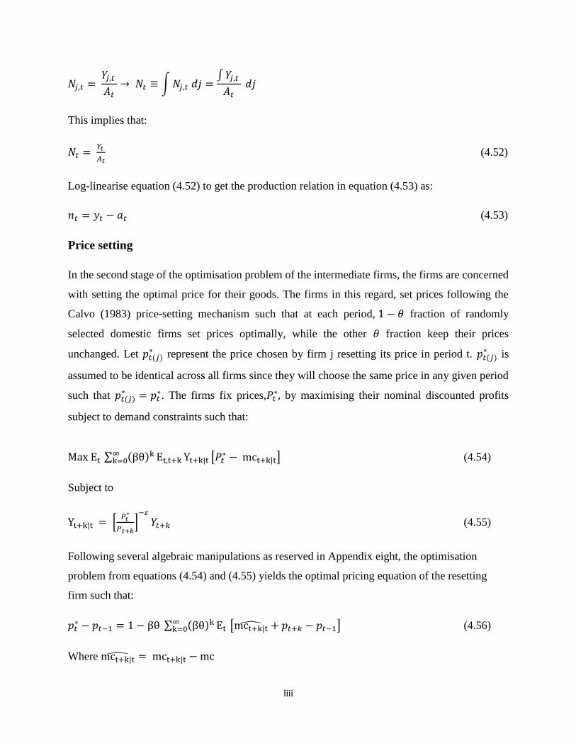
liii
𝑁𝑗,𝑡 = 𝑌𝑗,𝑡
𝐴𝑡→ 𝑁𝑡 ≡ ∫ 𝑁𝑗,𝑡 𝑑𝑗 =
∫ 𝑌𝑗,𝑡
𝐴𝑡 𝑑𝑗
This implies that:
𝑁𝑡 = 𝑌𝑡
𝐴𝑡 (4.52)
Log-linearise equation (4.52) to get the production relation in equation (4.53) as:
𝑛𝑡 = 𝑦𝑡 − 𝑎𝑡 (4.53)
Price setting
In the second stage of the optimisation problem of the intermediate firms, the firms are concerned
with setting the optimal price for their goods. The firms in this regard, set prices following the
Calvo (1983) price-setting mechanism such that at each period, 1 − 휃 fraction of randomly
selected domestic firms set prices optimally, while the other 휃 fraction keep their prices
unchanged. Let 𝑝𝑡(𝑗)∗ represent the price chosen by firm j resetting its price in period t. 𝑝𝑡(𝑗)
∗ is
assumed to be identical across all firms since they will choose the same price in any given period
such that 𝑝𝑡(𝑗)∗ = 𝑝𝑡
∗. The firms fix prices,𝑃𝑡∗, by maximising their nominal discounted profits
subject to demand constraints such that:
Max Et ∑ (βθ)k∞k=0 Et,t+k Yt+k|t [𝑃𝑡
∗ − mct+k|t] (4.54)
Subject to
Yt+k|t = [𝑃𝑡
∗
𝑃𝑡+𝑘]
−𝜀
𝑌𝑡+𝑘 (4.55)
Following several algebraic manipulations as reserved in Appendix eight, the optimisation
problem from equations (4.54) and (4.55) yields the optimal pricing equation of the resetting
firm such that:
𝑝𝑡∗ − 𝑝𝑡−1 = 1 − βθ ∑ (βθ)k Et
∞k=0 [mct+k|t + 𝑝𝑡+𝑘 − 𝑝𝑡−1] (4.56)
Where mct+k|t = mct+k|t − mc
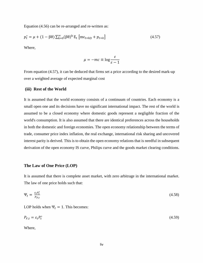
liv
Equation (4.56) can be re-arranged and re-written as:
𝑝𝑡∗ = 𝜇 + (1 − βθ) ∑ (βθ)k Et
∞k=0 [mct+k|t + 𝑝𝑡+𝑘] (4.57)
Where,
𝜇 = −𝑚𝑐 ≡ log휀
휀 − 1
From equation (4.57), it can be deduced that firms set a price according to the desired mark-up
over a weighted average of expected marginal cost
(iii) Rest of the World
It is assumed that the world economy consists of a continuum of countries. Each economy is a
small open one and its decisions have no significant international impact. The rest of the world is
assumed to be a closed economy where domestic goods represent a negligible fraction of the
world's consumption. It is also assumed that there are identical preferences across the households
in both the domestic and foreign economies. The open economy relationship between the terms of
trade, consumer price index inflation, the real exchange, international risk sharing and uncovered
interest parity is derived. This is to obtain the open economy relations that is needful in subsequent
derivation of the open economy IS curve, Philips curve and the goods market clearing conditions.
The Law of One Price (LOP)
It is assumed that there is complete asset market, with zero arbitrage in the international market.
The law of one price holds such that:
Ψ𝑡 = 𝜀𝑡𝑃𝑡
∗
𝑃𝐹,𝑡 (4.58)
LOP holds when Ψ𝑡 = 1. This becomes:
𝑃𝐹,𝑡 = 휀𝑡𝑃𝑡∗ (4.59)
Where,

lv
Ψ𝑡: Law of one price gap, LOP holds when Ψ𝑡 = 1
휀𝑡: Nominal Exchange rate
𝑃𝑡∗: World price index
𝑃𝐹,𝑡: Domestic price of imported goods
Log-linearising equation (4.59) yields:
𝑝𝐹,𝑡 = 𝑒𝑡 + 𝑝𝑡∗ (4.60)
Real Exchange Rate
The real exchange rate is defined as the ratio of the world price index to that of domestic price,
which is:
𝑄𝑡 = 𝜀𝑡𝑃𝑡
∗
𝑃𝐷,𝑡 (4.61)
Where,
𝑄𝑡: Real exchange rate
휀𝑡: Nominal Exchange rate
𝑃𝑡∗: World price index
𝑃𝐷,𝑡: Domestic price
The log-linearisation of equation (4.61) gives:
𝑞𝑡 = 𝑒𝑡 + 𝑝𝑡∗ − 𝑝𝐷,𝑡 (4.62)
Terms of Trade
The terms of trade between the domestic economy and foreign economy is defined as the ratio of
domestic prices (exports) to foreign prices (import). It measures the competitiveness of the
domestic economy such that:

lvi
𝑆𝑡 = 𝑃𝐷,𝑡
𝑃𝐹,𝑡 (4.63)
Where
𝑆𝑡: Terms of trade
𝑃𝐷,𝑡: Price of domestic goods
𝑃𝐹,𝑡: Price of foreign goods
The log-linearisation of the terms of trade in equation (4.63) will be:
𝑠𝑡 = 𝑝𝐷,𝑡 − 𝑝𝐹,𝑡 (4.64)
Domestic and Consumer Price Index (CPI) Inflation
The CPI Inflation is defined as the rate of change in the aggregate price index (that comprises the
domestic and foreign price index) while the domestic inflation is the rate of change in the domestic
price index. The log-linearisation of the Consumer Price Index, 𝑃𝑡 = (𝑃𝐷,𝑡)1−𝛼 + (𝑃𝐹,𝑡)𝛼 around
a symmetric steady state where the Purchasing Power Parity holds (i.e: 𝑃𝐷,𝑡 = 𝑃𝐹,𝑡) leads to:
𝑝𝑡 = (1 − 𝛼)𝑝𝐷,𝑡 + 𝛼𝑝𝐹,𝑡 (4.65)
Simplifying further, this becomes:
𝑝𝑡 = 𝑝𝐷,𝑡 − 𝛼(𝑝𝐷,𝑡 − 𝑝𝐹,𝑡) (4.66)
Since 𝑠𝑡 = 𝑝𝐷,𝑡 − 𝑝𝐹,𝑡 from equation (4.64), substitute it into equation (4.66) to get:
𝑝𝑡 = 𝑝𝐷,𝑡 − 𝛼(𝑠𝑡) (4.67)
Using a one-period lag, equation (4.67) becomes:
𝑝𝑡 − 𝑝𝑡−1 = 𝑝𝐷,𝑡 − 𝑝𝐷,𝑡−1 − 𝛼(𝑠𝑡 − 𝑠𝑡−1) (4.68)
Equation (4.68) can be re-written as:
𝜋𝑡 = 𝜋𝐷,𝑡 − 𝛼(∆ 𝑠𝑡) (4.69)

lvii
Equation (4.69) relates the CPI inflation (𝜋𝑡 = 𝑝𝑡 − 𝑝𝑡−1), domestic inflation (𝜋𝐷,𝑡 = 𝑝𝐷,𝑡 −
𝑝𝐷,𝑡−1) and the terms of trade (𝑠𝑡 = 𝑝𝐷,𝑡 − 𝑝𝐹,𝑡). It shows that the difference between the two
measures of inflation is proportional to changes in terms of trade. Parameter 𝛼 is the coefficient of
proportionality.
The link between the terms of trade and the law of one price
Next, equation (4.66) 𝑠𝑡 = 𝑝𝐷,𝑡 − 𝑝𝐹,𝑡which defines the terms of trade is combined with
equation (4.60) 𝑝𝐹,𝑡 = 𝑒𝑡 + 𝑝𝑡∗that depicts that the law of one price holds to give:
𝑠𝑡 = 𝑒𝑡 + 𝑝𝑡∗ − 𝑝𝐷,𝑡
Make 𝑒𝑡 the subject of the formula:
𝑒𝑡 = 𝑠𝑡 − 𝑝𝑡∗ + 𝑝𝐷,𝑡 (4.70)
Next, the relationship between the terms of trade and real exchange rate is derived. The real
exchange rate in equation (4.62) is imputed into equation (4.70) to give:
𝑞𝑡 = 𝑠𝑡 − 𝑝𝑡∗ + 𝑝𝐷,𝑡 + 𝑝𝑡
∗ − 𝑝𝑡
Simplifying, this becomes:
𝑞𝑡 = 𝑠𝑡 + 𝑝𝐷,𝑡 − 𝑝𝑡
Where 𝑝𝑡 = 𝑝𝐷,𝑡 − 𝛼(𝑠𝑡) as seen in equation (4.67) is substituted into the previous equation, this
becomes:
𝑞𝑡 = 𝑠𝑡 − 𝛼𝑠𝑡
𝑞𝑡 = (1 − 𝛼)𝑠𝑡 (4.71)
International Risk Sharing
In a complete and integrated international financial market, it is assumed that there is perfect risk
sharing between households in the domestic and foreign countries i.e. it is assumed that the prices
of domestic and foreign bonds are the same. It is also believed that the household in the domestic

lviii
and foreign economies share similar preferences. The first order conditions on consumption (4.23)
is combined with bond asset (4.25), one obtains:
𝛽 (𝐶𝑅,𝑡+1
𝐶𝑅,𝑡)
−𝜎𝑃𝑡
𝑃𝑡+1= 𝑄𝑡,𝑡+1 (4.72)
with the no-arbitrage condition
휀𝑡𝑄𝑡,𝑡+1∗ = 휀𝑡+1𝑄𝑡,𝑡+1 (4.73)
gives
𝛽 (𝐶𝑡+1
∗
𝐶𝑡∗ )
−𝜎 𝑃𝑡∗
𝑃𝑡+1∗ 휀𝑡 = 𝛽 (
𝐶𝑅,𝑡+1
𝐶𝑅,𝑡)
−𝜎𝑃𝑡
𝑃𝑡+1휀𝑡+1 (4.74)
Using equation (4.61) on the real exchange rate:
𝑄𝑡 = 휀𝑡𝑃𝑡
∗
𝑃𝑡
Equation (4.74) becomes:
(𝐶𝑡+1
∗
𝐶𝑡∗ )
−𝜎 𝑄𝑡
𝑄𝑡+1= (
𝐶𝑅,𝑡+1
𝐶𝑅,𝑡)
−𝜎
(4.75)
After re-arranging equation (4.75), it becomes:
𝐶𝑅,𝑡 = 𝐾𝐶𝑡∗𝑄𝑡
1
𝜎 (4.76)
Where 𝐾 =𝐶𝑅,𝑡+1
𝐶𝑡+1∗ 𝑄𝑡+1
−1
𝜎
Log-linearise equation (4.76), that is:
𝑐𝑅,𝑡 = 𝑐𝑡∗+
1
𝜎𝑞𝑡 (4.77)
Recall from equation (4.71) that 𝑞𝑡 = (1 − 𝛼)𝑠𝑡, then equation (4.77) becomes:
𝑐𝑅,𝑡 = 𝑐𝑡∗+
1−𝛼
𝜎𝑠𝑡 (4.78)
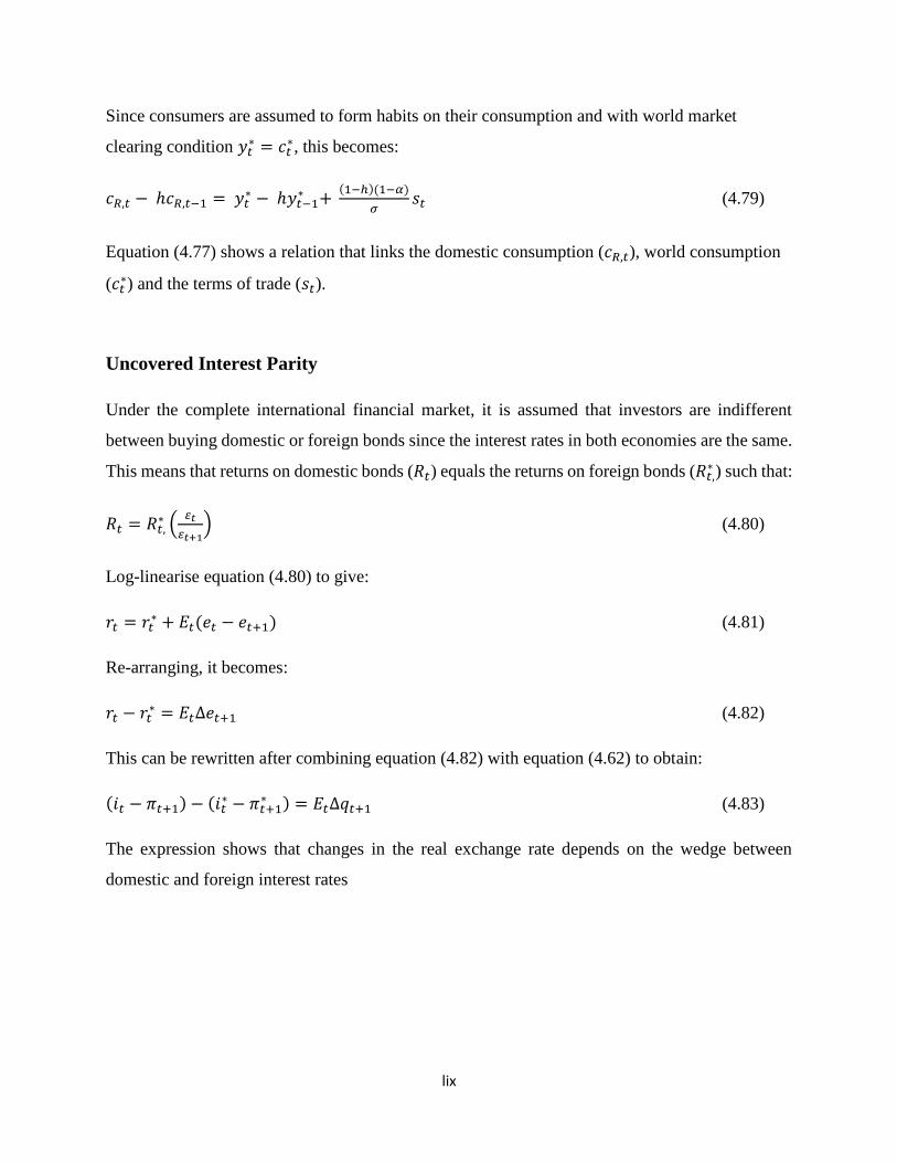
lix
Since consumers are assumed to form habits on their consumption and with world market
clearing condition 𝑦𝑡∗ = 𝑐𝑡
∗, this becomes:
𝑐𝑅,𝑡 − ℎ𝑐𝑅,𝑡−1 = 𝑦𝑡∗ − ℎ𝑦𝑡−1
∗ + (1−ℎ)(1−𝛼)
𝜎𝑠𝑡 (4.79)
Equation (4.77) shows a relation that links the domestic consumption (𝑐𝑅,𝑡), world consumption
(𝑐𝑡∗) and the terms of trade (𝑠𝑡).
Uncovered Interest Parity
Under the complete international financial market, it is assumed that investors are indifferent
between buying domestic or foreign bonds since the interest rates in both economies are the same.
This means that returns on domestic bonds (𝑅𝑡) equals the returns on foreign bonds (𝑅𝑡,∗ ) such that:
𝑅𝑡 = 𝑅𝑡,∗ (
𝜀𝑡
𝜀𝑡+1) (4.80)
Log-linearise equation (4.80) to give:
𝑟𝑡 = 𝑟𝑡∗ + 𝐸𝑡(𝑒𝑡 − 𝑒𝑡+1) (4.81)
Re-arranging, it becomes:
𝑟𝑡 − 𝑟𝑡∗ = 𝐸𝑡∆𝑒𝑡+1 (4.82)
This can be rewritten after combining equation (4.82) with equation (4.62) to obtain:
(𝑖𝑡 − 𝜋𝑡+1) − (𝑖𝑡∗ − 𝜋𝑡+1
∗ ) = 𝐸𝑡∆𝑞𝑡+1 (4.83)
The expression shows that changes in the real exchange rate depends on the wedge between
domestic and foreign interest rates

lx
Exogenous Processes in the Foreign Economy
Nigeria is assumed to be a small open economy relative to the large global economy and can
barely affect large foreign economies with respect to their interest rate, inflation and output. The
foreign variables are modelled as exogenous and follow AR(1) processes such that:
Foreign Output: 𝑦𝑡∗ = 𝜌𝑦𝑡
∗𝑦𝑡−1∗ + εt
𝑦𝑡∗ (4.84)
Foreign Inflation:𝜋𝑡∗ = 𝜌𝜋𝑡
∗𝜋𝑡−1∗ + εt
𝜋𝑡∗ (4.85)
Foreign Interest rate: 𝑟𝑡∗ = 𝜌 𝑟𝑡
∗ 𝑟𝑡−1∗ + εt
𝑟𝑡∗ (4.86)
The stochastic processes,휀𝑡𝑖~𝑖𝑖𝑁(0, 𝜎𝑖
2)
𝑓𝑜𝑟 𝑖 = 𝑦𝑡∗, 𝜋𝑡
∗, 𝑟𝑡∗. This means that the stochastic processes of foreign output, inflation and interest
rate are identically, independently and normally distributed of zero mean and variance of 𝜎𝑖2.
(iv) The Monetary Authority
The fourth agent in the model is now discussed. The Central Bank of Nigeria is assumed to follow
a simple Taylor-type rule i.e. the Central Bank implements monetary policy using the interest rate.
The CBN, under this rule, sets the interest rate by considering past value of interest rate, the
deviation of inflation, output and exchange rate from target
Rt
R= [
Rt−1
R]
ρR
[(πt
π)
υπ
(Yt
Y)
υY
(et
e)
υe
]1−ρR
sr,t (4.87)
Where,
Rt: Nominal interest rate
Rt−1: lagged interest rate
πt: Inflation rate
Yt: Output
et: Exchange rate
sr,t: Innovation to monetary policy
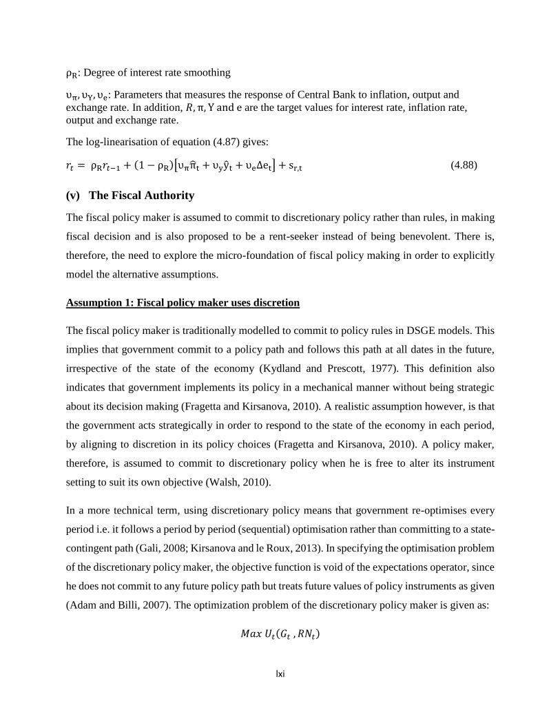
lxi
ρR: Degree of interest rate smoothing
υπ, υY, υe: Parameters that measures the response of Central Bank to inflation, output and
exchange rate. In addition, 𝑅, π, Y and e are the target values for interest rate, inflation rate,
output and exchange rate.
The log-linearisation of equation (4.87) gives:
𝑟𝑡 = ρR𝑟𝑡−1 + (1 − ρR)[υππt + υyyt + υe∆et] + sr,t (4.88)
(v) The Fiscal Authority
The fiscal policy maker is assumed to commit to discretionary policy rather than rules, in making
fiscal decision and is also proposed to be a rent-seeker instead of being benevolent. There is,
therefore, the need to explore the micro-foundation of fiscal policy making in order to explicitly
model the alternative assumptions.
Assumption 1: Fiscal policy maker uses discretion
The fiscal policy maker is traditionally modelled to commit to policy rules in DSGE models. This
implies that government commit to a policy path and follows this path at all dates in the future,
irrespective of the state of the economy (Kydland and Prescott, 1977). This definition also
indicates that government implements its policy in a mechanical manner without being strategic
about its decision making (Fragetta and Kirsanova, 2010). A realistic assumption however, is that
the government acts strategically in order to respond to the state of the economy in each period,
by aligning to discretion in its policy choices (Fragetta and Kirsanova, 2010). A policy maker,
therefore, is assumed to commit to discretionary policy when he is free to alter its instrument
setting to suit its own objective (Walsh, 2010).
In a more technical term, using discretionary policy means that government re-optimises every
period i.e. it follows a period by period (sequential) optimisation rather than committing to a state-
contingent path (Gali, 2008; Kirsanova and le Roux, 2013). In specifying the optimisation problem
of the discretionary policy maker, the objective function is void of the expectations operator, since
he does not commit to any future policy path but treats future values of policy instruments as given
(Adam and Billi, 2007). The optimization problem of the discretionary policy maker is given as:
𝑀𝑎𝑥 𝑈𝑡(𝐺𝑡 , 𝑅𝑁𝑡)
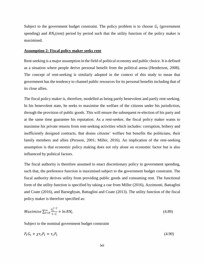
lxii
Subject to the government budget constraint. The policy problem is to choose 𝐺𝑡 (government
spending) and 𝑅𝑁𝑡(rent) period by period such that the utility function of the policy maker is
maximised.
Assumption 2: Fiscal policy maker seeks rent
Rent-seeking is a major assumption in the field of political economy and public choice. It is defined
as a situation where people derive personal benefit from the political arena (Henderson, 2008).
The concept of rent-seeking is similarly adopted in the context of this study to mean that
government has the tendency to channel public resources for its personal benefits including that of
its close allies.
The fiscal policy maker is, therefore, modelled as being partly benevolent and partly rent-seeking.
In his benevolent state, he seeks to maximise the welfare of the citizens under his jurisdiction,
through the provision of public goods. This will ensure the subsequent re-election of his party and
at the same time guarantee his reputation. As a rent-seeker, the fiscal policy maker wants to
maximise his private returns from rent-seeking activities which includes: corruption, bribery and
inefficiently designed contracts, that drains citizens’ welfare but benefits the politicians, their
family members and allies (Persson, 2001; Miller, 2016). An implication of the rent-seeking
assumption is that economic policy making does not rely alone on economic factor but is also
influenced by political factors.
The fiscal authority is therefore assumed to enact discretionary policy in government spending,
such that, the preference function is maximised subject to the government budget constraint. The
fiscal authority derives utility from providing public goods and consuming rent. The functional
form of the utility function is specified by taking a cue from Miller (2016), Azzimonti, Battaglini
and Coate (2016), and Barseghyan, Battaglini and Coate (2013). The utility function of the fiscal
policy maker is therefore specified as:
𝑀𝑎𝑥𝑖𝑚𝑖𝑠𝑒 ∑𝐺𝑡
1−𝜁
1−𝜁∞𝑡=0 + ln 𝑅𝑁𝑡 (4.89)
Subject to the nominal government budget constraint
𝑃𝑡𝐺𝑡 + 𝜒𝜏𝑡𝑃𝑡 = 𝜏𝑡𝑃𝑡 (4.90)

lxiii
Where,
𝐺𝑡: Government provision of public goods
𝑅𝑁𝑡: Rent received. Rent received is defined to depend on the propensity of public office holders
to seek rent and the total revenue that the government generates. It is defined as:
𝑅𝑁𝑡 = 𝜒𝜏𝑡 (4.91)
where 𝜒 𝑖𝑠 the degree of rent seeking. 𝜒 < 0 ≤ 1; the degree of rent seeking increases as
𝜒 → 0. 𝜏𝑡 is the total government revenue
휁: Institutional Parameter, when 휁 → 1, the political institution is strong and when 휁 → 0, there is
weak political institution.
Equation (4.89) is subject to the nominal government budget constraint (equation 4.90). The
constraint shows that the total spending of government in form of rents accrued to government and
allies and on the provision of public goods equals total revenue of government taxes.
𝑃𝑡𝐺𝑡 + 𝜒𝜏𝑡𝑃𝑡 = 𝜏𝑡𝑃𝑡
Where,
𝐺𝑡: Government spending
𝜒𝜏𝑡: Rent raised
𝜏𝑡: Total Revenue
𝑃𝑡: Nominal price
As usual, the Lagrangian function of the maximisation problem from equations (4.89) and (4.90)
is such that:
ℒ = ∑𝐺𝑡
1−𝜁
1−𝜁∞𝑡=0 + ln 𝑅𝑁𝑡 + 𝜆𝑡[𝜏𝑡𝑃𝑡 − 𝑃𝑡𝐺𝑡 − 𝜒𝜏𝑡𝑃𝑡] (4.92)
In the same manner, first order condition (F.O.C) of equation (4.92) is obtained as follows:
Government Spending: 𝜕ℒ
𝜕𝐺𝑡= 0: 𝐺𝑡
−𝜁= −𝜆𝑡𝑃𝑡 (4.93)

lxiv
Rent: 𝜕ℒ
𝜕𝑅𝑁𝑡= 0:
1
𝑅𝑁𝑡= −𝜆𝑡𝑃𝑡 (4.94)
𝜆𝑡: 𝜕ℒ
𝜕𝜆𝑡= 0: 𝜏𝑡𝑃𝑡 = 𝑃𝑡𝐺𝑡 + 𝜒𝜏𝑡𝑃𝑡 (4.95)
Equations (4.93) and (4.94) are combined to give equation (4.96):
𝐺𝑡−𝜁
=1
𝑅𝑁𝑡 (4.96)
Equation (4.96) is then re-arranged to be:
𝐺𝑡𝜁
= 𝑅𝑁𝑡 (4.97)
Equation (4.97) gives:
𝐺𝑡 = (𝜒𝜏𝑡)1
𝜁 (4.98)
In equation (4.98), government spending policy 𝐺𝑡 at time t depends on the degree of rent seeking
(𝜒), the quality of political institution (휁) and government revenue.
Equation (4.98) is then log-linearised as:
𝑔𝑡 =1
𝜁(𝜒𝜏𝑡) (4.99)
Assumption 3: There is no or weak policy coordination
This third assumption is implicitly modelled by assuming that both fiscal and monetary authorities
are adopting different policy regimes-discretion or rules. In the case of this study, the government
is pursuing a discretionary regime while the Central Bank is following a rule-based regime.
(vi) Exogenous Shock Processes
In the model adopted for this study, eleven sources of exogenous shocks are considered. They
include: innovation in technology, monetary policy, government spending, foreign inflation,
foreign output and foreign interest rate, tax, rent seeking, output, domestic inflation and transfer
payment. The equations of these shocks can be expressed as follows:
Technology:𝑎𝑡 = 𝜌𝑎𝑎𝑡−1 + 휀𝑡𝑎 (4.100)

lxv
Monetary Policy:stR = 𝜌𝑟𝑠𝑟𝑡−1 + 휀𝑡
𝑟 (4.101)
Government Spending: stG = 𝜌𝑔𝑠𝑔𝑡−1 + 휀𝑡
𝑔 (4.102)
Tax: 𝜏𝑡 = 𝜌𝜏𝜏𝑡−1 + 휀𝑡𝜏 (4.103)
Output: sty
= 𝜌𝑦𝑠𝑦𝑡−1 + 휀𝑡𝑦
(4.104)
Domestic Inflation: stπD = 𝜌𝜋𝑠𝜋𝑡−1 + 휀𝑡
𝜋𝐷 (4.105)
Rent seeking: 𝑟𝑛𝑡 = 𝜌𝑟𝑛𝑟𝑛𝑡−1 + 휀𝑡𝑟𝑛 (4.106)
Transfer payment: 𝑇𝑃𝑡 = 𝜌𝑇𝑃𝑇𝑃𝑡−1 + 휀𝑡𝑇𝑃 (4.40)
Foreign Output: 𝑦𝑡∗ = 𝜌𝑦𝑡
∗𝑦𝑡−1∗ + εt
𝑦𝑡∗ (4.84)
Foreign Inflation:𝜋𝑡∗ = 𝜌𝜋𝑡
∗𝜋𝑡−1∗ + εt
𝜋𝑡∗ (4.85)
Foreign Interest rate: 𝑟𝑡∗ = 𝜌 𝑟𝑡
∗ 𝑟𝑡−1∗ + εt
𝑟𝑡∗ (4.86)
Where,휀𝑡𝑗~𝑖𝑖𝑁(0, 𝜎𝑖
2)
𝑓𝑜𝑟 𝑗 = 𝑎, 𝑟, 𝑦𝑡∗, 𝜋𝑡
∗, 𝑟𝑡∗, 𝑔𝑡, 𝑇𝑃, 𝑟𝑛, 𝜏, 𝑦, 𝜋
(vii) Aggregation Rules
According to Adegboye (2015), the following aggregation rules for consumption and labour
supply over the Ricardian and non-Ricardian households are specified. Aggregate consumption
for both Ricardian and non-Ricardian agents is given by:
ct = ψ cR,t + (1 − ψ)cNR,t (4.106)
Aggregate labour supply for both Ricardian and non-Ricardian agents is given by:
nt = ω nR,t + (1 − ω)nNR,t (4.107)
Total inflation is also given by the sum of domestic inflation and foreign inflation, such that:
𝜋𝑡 = 𝜋𝐷,𝑡 + 𝜋𝐹,𝑡 (4.108)
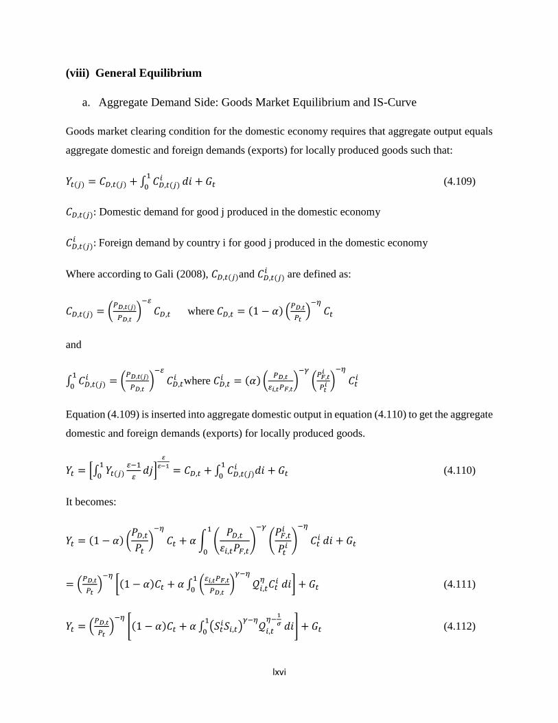
lxvi
(viii) General Equilibrium
a. Aggregate Demand Side: Goods Market Equilibrium and IS-Curve
Goods market clearing condition for the domestic economy requires that aggregate output equals
aggregate domestic and foreign demands (exports) for locally produced goods such that:
𝑌𝑡(𝑗) = 𝐶𝐷,𝑡(𝑗) + ∫ 𝐶𝐷,𝑡(𝑗)𝑖1
0𝑑𝑖 + 𝐺𝑡 (4.109)
𝐶𝐷,𝑡(𝑗): Domestic demand for good j produced in the domestic economy
𝐶𝐷,𝑡(𝑗)𝑖 : Foreign demand by country i for good j produced in the domestic economy
Where according to Gali (2008), 𝐶𝐷,𝑡(𝑗)and 𝐶𝐷,𝑡(𝑗)𝑖 are defined as:
𝐶𝐷,𝑡(𝑗) = (𝑃𝐷,𝑡(𝑗)
𝑃𝐷,𝑡)
−𝜀
𝐶𝐷,𝑡 where 𝐶𝐷,𝑡 = (1 − 𝛼) (𝑃𝐷,𝑡
𝑃𝑡)
−𝜂
𝐶𝑡
and
∫ 𝐶𝐷,𝑡(𝑗)𝑖1
0= (
𝑃𝐷,𝑡(𝑗)
𝑃𝐷,𝑡)
−𝜀
𝐶𝐷,𝑡𝑖 where 𝐶𝐷,𝑡
𝑖 = (𝛼) (𝑃𝐷,𝑡
𝜀𝑖,𝑡𝑃𝐹,𝑡)
−𝛾
(𝑃𝐹,𝑡
𝑖
𝑃𝑡𝑖 )
−𝜂
𝐶𝑡𝑖
Equation (4.109) is inserted into aggregate domestic output in equation (4.110) to get the aggregate
domestic and foreign demands (exports) for locally produced goods.
𝑌𝑡 = [∫ 𝑌𝑡(𝑗)𝜀−1
𝜀𝑑𝑗
1
0]
𝜀
𝜀−1= 𝐶𝐷,𝑡 + ∫ 𝐶𝐷,𝑡(𝑗)
𝑖 𝑑𝑖1
0+ 𝐺𝑡 (4.110)
It becomes:
𝑌𝑡 = (1 − 𝛼) (𝑃𝐷,𝑡
𝑃𝑡)
−𝜂
𝐶𝑡 + 𝛼 ∫ (𝑃𝐷,𝑡
휀𝑖,𝑡𝑃𝐹,𝑡)
−𝛾
(𝑃𝐹,𝑡
𝑖
𝑃𝑡𝑖
)
−𝜂
𝐶𝑡𝑖
1
0
𝑑𝑖 + 𝐺𝑡
= (𝑃𝐷,𝑡
𝑃𝑡)
−𝜂
[(1 − 𝛼)𝐶𝑡 + 𝛼 ∫ (𝜀𝑖,𝑡𝑃𝐹,𝑡
𝑃𝐷,𝑡)
𝛾−𝜂
𝒬𝑖,𝑡𝜂
𝐶𝑡𝑖 𝑑𝑖
1
0] + 𝐺𝑡 (4.111)
𝑌𝑡 = (𝑃𝐷,𝑡
𝑃𝑡)
−𝜂
[(1 − 𝛼)𝐶𝑡 + 𝛼 ∫ (𝑆𝑡𝑖𝑆𝑖,𝑡)
𝛾−𝜂𝒬
𝑖,𝑡
𝜂−1
𝜎 𝑑𝑖1
0] + 𝐺𝑡 (4.112)
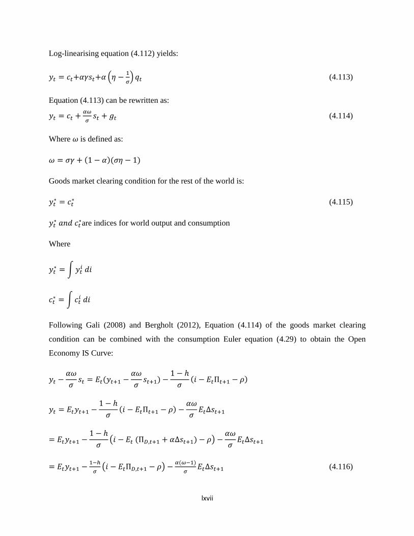
lxvii
Log-linearising equation (4.112) yields:
𝑦𝑡 = 𝑐𝑡+𝛼𝛾𝑠𝑡+𝛼 (휂 −1
𝜎) 𝑞𝑡 (4.113)
Equation (4.113) can be rewritten as:
𝑦𝑡 = 𝑐𝑡 +𝛼𝜔
𝜎𝑠𝑡 + 𝑔𝑡 (4.114)
Where 𝜔 is defined as:
𝜔 = 𝜎𝛾 + (1 − 𝛼)(𝜎휂 − 1)
Goods market clearing condition for the rest of the world is:
𝑦𝑡∗ = 𝑐𝑡
∗ (4.115)
𝑦𝑡∗ 𝑎𝑛𝑑 𝑐𝑡
∗are indices for world output and consumption
Where
𝑦𝑡∗ = ∫ 𝑦𝑡
𝑖 𝑑𝑖
𝑐𝑡∗ = ∫ 𝑐𝑡
𝑖 𝑑𝑖
Following Gali (2008) and Bergholt (2012), Equation (4.114) of the goods market clearing
condition can be combined with the consumption Euler equation (4.29) to obtain the Open
Economy IS Curve:
𝑦𝑡 −𝛼𝜔
𝜎𝑠𝑡 = 𝐸𝑡(𝑦𝑡+1 −
𝛼𝜔
𝜎𝑠𝑡+1) −
1 − ℎ
𝜎(𝑖 − 𝐸𝑡Π𝑡+1 − 𝜌)
𝑦𝑡 = 𝐸𝑡𝑦𝑡+1 −1 − ℎ
𝜎(𝑖 − 𝐸𝑡Π𝑡+1 − 𝜌) −
𝛼𝜔
𝜎𝐸𝑡∆𝑠𝑡+1
= 𝐸𝑡𝑦𝑡+1 −1 − ℎ
𝜎(𝑖 − 𝐸𝑡 (Π𝐷,𝑡+1 + 𝛼∆𝑠𝑡+1) − 𝜌) −
𝛼𝜔
𝜎𝐸𝑡∆𝑠𝑡+1
= 𝐸𝑡𝑦𝑡+1 −1−ℎ
𝜎(𝑖 − 𝐸𝑡Π𝐷,𝑡+1 − 𝜌) −
𝛼(𝜔−1)
𝜎𝐸𝑡∆𝑠𝑡+1 (4.116)

lxviii
Where Θ = (𝜔 − 1)
Insert 𝑦𝑡 = 𝑦𝑡∗ +
1
𝜎𝛼𝑠𝑡 into equation (4.116) to get the open economy IS curve
𝑦𝑡 = 𝐸𝑡𝑦𝑡+1 −1−ℎ
𝜎𝛼(𝑖 − 𝐸𝑡Π𝐷,𝑡+1 − 𝜌) − 𝛼Θ 𝐸𝑡 (∆𝑦𝑡+1
∗ ) (4.117)
Under the assumption of flexible prices, equation (4.117) is written as
𝑦𝑡𝑛 = 𝐸𝑡𝑦𝑡+1
𝑛 −1−ℎ
𝜎𝛼(𝑟𝑡
𝑛 − 𝜌) − 𝛼Θ 𝐸𝑡 (∆𝑦𝑡+1∗ ) (4.118)
Subtract equation (4.118) from (4.117) to obtain the dynamic IS curve:
𝑦�� = 𝐸𝑡��𝑡+1 −1−ℎ
𝜎𝛼(𝑖 − 𝐸𝑡Π𝐷,𝑡+1 − 𝑟𝑡
𝑛) (4.119)
b. Aggregate Supply Side: Marginal Cost and Open Economy New Keynesian
Philips Curve
Recall that the optimal price setting condition of the firm in equation (4.56) is given as:
𝑝𝑡∗ − 𝑝𝑡−1 = 1 − βθ ∑ (βθ)k Et
∞k=0 [mct+k|t + 𝑝𝑡+𝑘 − 𝑝𝑡−1]
mct+k|t = 𝑚𝑐𝑡+𝑘|𝑡 − 𝑚𝑐𝑡+𝑘
Equation (4.56) is simplified further to yield:
𝑝𝑡∗ − 𝑝𝑡−1 = βθ Et [𝑝𝑡+1
∗ − 𝑝𝑡] + (1 − βθ)mct + πt (4.120)
Dynamics of the aggregate price index
The law of motion for the aggregate price index is:
��𝑡 = [휃(𝑃𝑡−1)1−𝜀 + (1 − 휃)(𝑃𝑡∗)1−𝜀]
1
1−𝜀 (4.121)
This becomes
(��𝑡)1−𝜀 = [휃(𝑃𝑡−1)1−𝜀 + (1 − 휃)(𝑃𝑡∗)1−𝜀] (4.122)
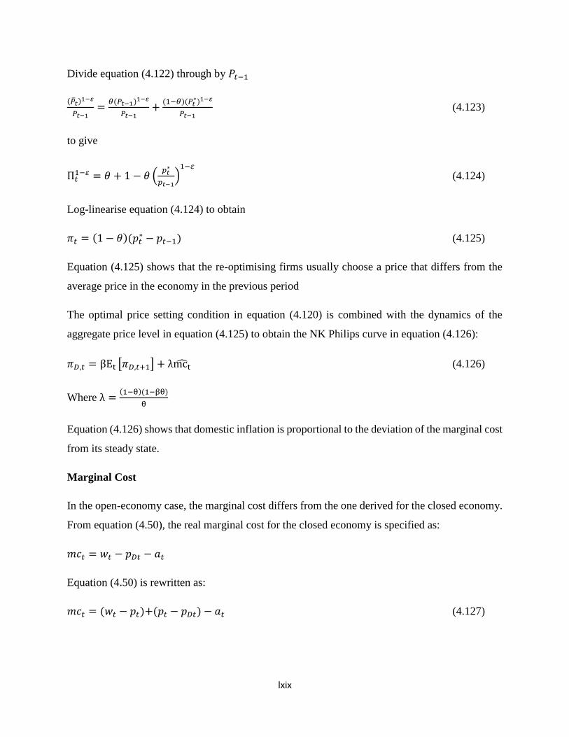
lxix
Divide equation (4.122) through by 𝑃𝑡−1
(��𝑡)1−𝜀
𝑃𝑡−1=
𝜃(𝑃𝑡−1)1−𝜀
𝑃𝑡−1+
(1−𝜃)(𝑃𝑡∗)1−𝜀
𝑃𝑡−1 (4.123)
to give
Π𝑡1−𝜀 = 휃 + 1 − 휃 (
𝑝𝑡∗
𝑝𝑡−1)
1−𝜀
(4.124)
Log-linearise equation (4.124) to obtain
𝜋𝑡 = (1 − 휃)(𝑝𝑡∗ − 𝑝𝑡−1) (4.125)
Equation (4.125) shows that the re-optimising firms usually choose a price that differs from the
average price in the economy in the previous period
The optimal price setting condition in equation (4.120) is combined with the dynamics of the
aggregate price level in equation (4.125) to obtain the NK Philips curve in equation (4.126):
𝜋𝐷,𝑡 = βEt [𝜋𝐷,𝑡+1] + λmct (4.126)
Where λ =(1−θ)(1−βθ)
θ
Equation (4.126) shows that domestic inflation is proportional to the deviation of the marginal cost
from its steady state.
Marginal Cost
In the open-economy case, the marginal cost differs from the one derived for the closed economy.
From equation (4.50), the real marginal cost for the closed economy is specified as:
𝑚𝑐𝑡 = 𝑤𝑡 − 𝑝𝐷𝑡 − 𝑎𝑡
Equation (4.50) is rewritten as:
𝑚𝑐𝑡 = (𝑤𝑡 − 𝑝𝑡)+(𝑝𝑡 − 𝑝𝐷𝑡) − 𝑎𝑡 (4.127)

lxx
Equation (4.67) which shows that the difference between the aggregate price and domestic price
is proportional to the terms of trade: 𝑝𝑡 = 𝑝𝐷,𝑡 − 𝛼𝑠𝑡 and the labour supply schedule in equation
(4.32): 𝑤𝑡 − 𝑝𝑡 = 𝜎𝑐𝑡 + 𝜑𝑛𝑡 is inserted into equation (4.127) to get:
𝑚𝑐𝑡 = 𝜎𝑐𝑡 + 𝜑𝑛𝑡 + 𝛼𝑠𝑡 − 𝑎𝑡 (4.128)
The next step is to insert the international risk sharing condition in equation (4.83) and the
production relation in equation (4.54) into equation (4.128). This will yield:
𝑚𝑐𝑡 = 𝜎 [𝑐𝑡∗ +
1−𝛼
𝜎𝑠𝑡] + 𝜑[𝑦𝑡 − 𝑎𝑡] + 𝛼𝑠𝑡 − 𝑎𝑡 (4.129)
With the world market clearing condition 𝑦𝑡∗ = 𝑐𝑡
∗, equation (4.129) can be rewritten as:
𝑚𝑐𝑡 = 𝜎𝑦𝑡∗ + 𝜑𝑦𝑡 + 𝑠𝑡 − (1 + 𝜑)𝑎𝑡 (4.130)
𝑦𝑡 = 𝑦𝑡∗ +
1
𝜎𝛼𝑠𝑡 is inserted into equation (4.130). This becomes:
𝑚𝑐𝑡 = (𝜎𝛼 + 𝜑)𝑦𝑡 + (𝜎 − 𝜎𝛼)𝑦𝑡∗ − (1 + 𝜑)𝑎𝑡 (4.131)
Equation (4.131) is rewritten in the flexible price version as:
𝑚𝑐 = (𝜎𝛼 + 𝜑)𝑦𝑡𝑛 + (𝜎 − 𝜎𝛼)𝑦𝑡
∗ − (1 + 𝜑)𝑎𝑡 (4.132)
Equation (4.132) is subtracted from equation (4.131) to obtain the real marginal cost gap:
𝑚�� = (𝜎𝛼 + 𝜑)𝑦�� (4.133)
Equation (4.133) is imputed into equation (4.126) 𝜋𝐷,𝑡 = βEt [𝜋𝐷,𝑡+1] + λmct
Where λ =(1−θ)(1−βθ)
θ in order to derive the open-economy NK Philips curve equation as
specified in equation (4.134) as:
𝜋𝐷,𝑡 = βEt [𝜋𝐷,𝑡+1] + kα𝑦�� (4.134)
Where
kα = λ(𝜎𝛼 + 𝜑) =(1 − θ)(1 − βθ)
θ(𝜎𝛼 + 𝜑)

lxxi
4.2.2 Solving and Estimating the Open Economy NK DSGE model
In this sub-section, the steps to solving and estimating the DSGE model adopted for this study are
presented. These involve three procedures that comprise the log-linearisation of the model, then
solving a system of linear difference equations derived from the model and lastly, the Bayesian
estimation of the model.
1. Log-Linearise the model
The set of equations of the DSGE model as specified in sub-section 4.2.1 are represented in a
canonical form as:
𝐸𝑡{𝑓(𝑦𝑡+1, 𝑦𝑡 , 𝑦𝑡−1, 𝑒𝑡} = 1 (4.135)
Where,
𝑦𝑡: Vector of endogenous variables of the model. There are current, lead and lag values of the
endogenous variable
yt−1: Vector of predetermined variables
𝑒𝑡: Vector of stochastic exogenous variables, 𝑒𝑡~𝑖𝑖𝑁(0, 𝜎𝑖2)
DSGE models often lack an exact and closed form solution that can be cumbersome and messy
with paper and pencil. The solution to the DSGE model in equation (4.135) is derived by
approximating the non-linear set of equations. The existing approximation methods are classified
as either the Perturbation or Projection Methods. The Perturbation solutions are local approximants
that usually involves a Taylor series approximation of equilibrium equations around their non-
stochastic steady state. Fernandez-Villaverde, Rubio-Ramirez and Schorfheide (2016) argue that
perturbation methods are most suitable for solving a medium-scale NK model since it is
sufficiently well behaved. Linear Quadratic method, linear approximation and Second (or Higher)
Order Approximation are some Perturbation methods. Projections methods on the other hand, have
global solutions. In this study, one of the perturbation method is used, specifically, the log-linear
approximation method.
The log-linear approximation method approximates the solution to equation (4.135) in terms of
the log-deviations of the variables with respect to their steady state. In general, it is adequate for
several economic analyses since it leads to a state-space representation of the model, which is

lxxii
suitable for empirical estimation and forecasting. Log-linear solutions are easy to read, the
coefficient terms are interpreted as elasticity and, in some circumstances, they can improve the
accuracy of the solution (Fernandez-Villaverde, Rubio-Ramirez and Schorfheide, 2016). The
procedure of log-linearising begins with finding the steady state of the model where there are no
exogenous shocks and variables have no time sub-scripts such that,
{𝑓(��, ��, ��, 0} = 1 (4.136)
Equation (4.135) is thereafter approximated by a first-order Taylor expansion of its logarithm
around the steady-state (4.136) such that,
𝐸𝑡{𝑓𝑦𝑡+1 ��𝑡+1, 𝑓𝑦𝑡
𝑦��, 𝑓𝑦𝑡−1��𝑡−1, 𝑓𝑒𝑒𝑡} = 1 (4.137)
Equation (4.137) is the approximated linear model.

lxxiii
4.2.3 System of Equations to be estimated
After obtaining the optimisation result of each sector of the economy, the relevant equations to
be estimated are presented in Tables 4.1 and 4.2. They are as follows:
Table 4.1: Log-linear System of Equations
S/N Name Equations Source
Equation
1.
Ricardian
Consumption
𝒄𝑹,𝒕 − 𝒉𝒄𝑹,𝒕−𝟏 = 𝑬𝒕(𝒄𝑹,𝒕+𝟏 − 𝒉𝒄𝑹,𝒕)
−𝟏 − 𝒉
𝝈(𝒓 − 𝑬𝒕𝚷𝒕+𝟏)
Where,
𝚷𝒕+𝟏 = 𝑷𝒕+𝟏 − 𝑷𝒕
4.29
2. Non- Ricardian
Consumption
𝒄𝑵𝑹,𝒕 =𝑾𝑵
𝑷𝑪(𝒘𝒕 − 𝒑𝒕 + 𝒏𝑵𝑹,𝒕) +
𝑻𝑷
𝑷𝑪(𝒕𝒑𝒕)
4.39
3.
4.
5.
Labour Supply
schedule for
Non- Ricardian
Household
Transfer to non-
Ricardian
household
Marginal cost
𝒘𝒕 − 𝒑𝒕 =𝝈
𝟏 − 𝒉(𝒄𝑵𝑹,𝒕 − 𝒉𝒄𝑵𝑹,𝒕−𝟏) + 𝝋𝒏𝒕
𝑻𝑷𝒕 = 𝝆𝑻𝑷𝑻𝑷𝒕−𝟏 + 𝜺𝒕𝑻𝑷
𝒎𝒄𝒕 = 𝒘𝒕 − 𝒑𝒕 − 𝒂𝒕
4.41
4.40
4.50
6.
Aggregate
Consumption
𝒄𝒕 = 𝝍𝒄𝑹,𝒕 + (𝟏 − 𝝍)𝒄 𝑵𝑹,𝒕 4.106

lxxiv
Table 4.1
(Continued
)
S/N Name Equations Equation
Number
7. Domestic Goods
Market clearing
𝒚𝒕 = 𝒄𝒕 +𝜶𝝎
𝝈𝒔𝒕 + 𝒈𝒕 + 𝒔𝒚,𝒕
Where
𝝎 = 𝝈𝜸 + (𝟏 − 𝜶)(𝝈𝜼 − 𝟏)
4.114
8. International
Risk Sharing
𝒄𝒕 − 𝒉𝒄𝒕−𝟏 = 𝒚𝒕∗ − 𝒉𝒚𝒕−𝟏
∗ + (𝟏 − 𝒉)(𝟏 − 𝜶)
𝝈𝒔𝒕
4.79
9.
10.
Domestic
Inflation
Total Inflation
𝝅𝑫,𝒕 = 𝛃𝐄𝐭 [𝝅𝑫,𝒕+𝟏] + 𝐤𝛂𝒚�� + 𝒔𝝅𝑫
Where
𝐤𝛂 = 𝛌(𝝈𝜶 + 𝝋) =(𝟏 − 𝛉)(𝟏 − 𝛃𝛉)
𝛉(𝝈𝜶 + 𝝋)
𝝅𝒕 = 𝝅𝑫,𝒕 + 𝝅𝑭,𝒕
4.134
4.108
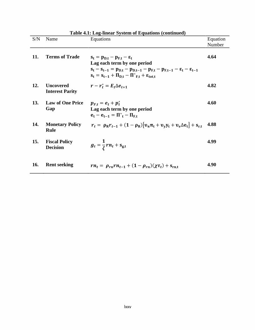
lxxv
Table 4.1: Log-linear System of Equations (continued)
S/N Name Equations Equation
Number
11.
Terms of Trade
𝐬𝐭 = 𝐩𝐃,𝐭 − 𝐩𝐅,𝐭 − 𝛆𝐭
Lag each term by one period
𝐬𝐭 − 𝐬𝐭−𝟏 = 𝐩𝐃,𝐭 − 𝐩𝐃,𝐭−𝟏 − 𝐩𝐅,𝐭 − 𝐩𝐅,𝐭−𝟏 − 𝛆𝐭 − 𝛆𝐭−𝟏
𝐬𝐭 = 𝐬𝐭−𝟏 + 𝚷𝐃,𝐭 − 𝚷∗𝐅,𝐭 + 𝛆𝐭𝐨𝐭,𝐭
4.64
12. Uncovered
Interest Parity
𝒓 − 𝒓𝒕∗ = 𝑬𝒕∆𝒆𝒕+𝟏 4.82
13. Law of One Price
Gap
𝒑𝑭,𝒕 = 𝒆𝒕 + 𝒑𝒕∗
Lag each term by one period
𝐞𝐭 − 𝐞𝐭−𝟏 = 𝚷∗𝐭 − 𝚷𝐅,𝐭
4.60
14. Monetary Policy
Rule
𝒓𝒕 = 𝛒𝐑𝒓𝒕−𝟏 + (𝟏 − 𝛒𝐑)[𝛖𝛑𝛑𝐭 + 𝛖𝐲𝐲𝐭 + 𝛖𝐞∆𝐞𝐭] + 𝐬𝐫,𝐭 4.88
15.
16.
Fiscal Policy
Decision
Rent seeking
𝒈𝒕 =𝟏
𝜻𝒓𝒏𝒕 + 𝐬𝐠,𝐭
𝒓𝒏𝒕 = 𝝆𝒓𝒏𝒓𝒏𝒕−𝟏 + (𝟏 − 𝝆𝒓𝒏)(𝝌𝝉𝒕) + 𝐬𝐫𝐧,𝐭
4.99
4.90

lxxvi
Table 4.2: Foreign Economy and other Exogenous Processes
S/N Name Equations Equation
Number
17. Foreign Output: 𝒚𝒕∗ = 𝝆𝒚𝒕
∗𝒚𝒕−𝟏∗ + 𝛆𝐭
𝒚𝒕∗ 4.84
18. Foreign Inflation :𝝅𝒕∗ = 𝝆𝝅𝒕
∗𝝅𝒕−𝟏∗ + 𝛆𝐭
𝝅𝒕∗
4.85
19. Foreign Interest
rate 𝒓𝒕
∗ = 𝝆 𝒓𝒕∗ 𝒓𝒕−𝟏
∗ + 𝛆𝐭 𝒓𝒕
∗
4.86
20.
21.
22.
23.
24.
25.
26.
27.
Technology
Monetary Policy
Government
Spending
Tax
Output
Domestic Inflation
Rent seeking
Transfer payment
𝒂𝒕 = 𝝆𝒂𝒂𝒕−𝟏 + 𝜺𝒕𝒂
𝐬𝐭𝐑 = 𝝆𝒔𝒓𝒔𝒓𝒕−𝟏 + 𝜺𝒕
𝒓
𝐬𝐭𝐆 = 𝝆𝒔𝒈𝒔𝒈𝒕−𝟏 + 𝜺𝒕
𝒈
𝝉𝒕 = 𝝆𝝉𝝉𝒕−𝟏 + 𝜺𝒕𝝉
𝐬𝐭𝐲
= 𝝆𝒔𝒚𝒔𝒚𝒕−𝟏 + 𝜺𝒕𝒚
𝐬𝐭𝛑𝐃 = 𝝆𝝅𝑫𝒔𝝅𝒕−𝟏 + 𝜺𝒕
𝝅𝑫
𝒔𝒓𝒏𝒕 = 𝝆𝒔𝒓𝒏𝒓𝒏𝒕−𝟏 + 𝜺𝒕𝒓𝒏
𝑻𝑷𝒕 = 𝝆𝑻𝑷𝑻𝑷𝒕−𝟏 + 𝜺𝒕𝑻𝑷
4.100
4.101
4.102
4.103
4.104
4.105
4.106
4.40
:

lxxvii
Table 4.3: List of Parameters estimated Symbol Parameters Distribution Mean Standard
deviation
Reference
H Habit formation Beta 0.70 0.10 Almeida (2010)
Sigma (𝜎) Inverse elasticity of
substitution
Normal 3.00 1.00 Cebi (2011)
Psi (𝜓) Share of non-Ricardian
household
Beta 0.70 0.10 Value informed by Iwata
(2009)
alpha (𝛼) Degree of openness Beta 0.40 0.10 average value of trade
openness in Nigeria (1960-
2015)
Phi (𝜑) Inverse elasticity of labour Normal 4.38 2.00 Adegboye (2015)
eta (휂) Elasticity of substitution
between home and foreign
goods
Gamma 11.42 1.00 Adegboye (2015)
Theta (휃) Calvo Price Stickiness Beta 0.50 0.10 Adegboye (2015)
upssilon_pii
(𝜐𝜋)
Taylor feedback on
Inflation
Gamma 1.50 0.20 Gali and Monacelli (2005)
upssilon_y
(𝜐𝑦)
Taylor feedback on Output Gamma 0.50 0.10 Gali (2008)
upssilon_ex
r (𝜐𝑒)
Taylor feedback on
exchange rate
Gamma 0.80 0.10 Adegboye (2015)
rrho_r (𝜌𝑟) Interest rate smoothening Beta 0.70 0.10 Serbaniou (2012)
chi (𝜒) Degree of rent- seeking Beta 0.50 0.10 Informed by data from
Corruption perception
Index and World
Governance Indicator
Zeta (휁) Quality of political
institutions
Beta 0.35 0.10 Informed by data from
Corruption perception
Index and World
Governance Indicator
rrho_ystar
(𝜌𝑦𝑠𝑡𝑎𝑟)
AR(1) of foreign output Beta 0.70 0.10 Informed by Traum and
Yang (2011) to depict
high persistence of shock
processes
rrho_a (𝜌𝑎) AR(1) of technology Beta 0.70 0.10 Informed by Traum and
Yang (2011) to depict
high persistence of shock
processes
Sources: Listed in table 4.3

lxxviii
Table 4.3 (continued): List of Parameters estimated Symbol Parameters Distribution Mean Standard
deviation
Reference
rrho_piiD
(𝜌𝜋𝐷)
AR(1) of inflation
shock
Beta 0.70 0.10 Informed by Traum and
Yang (2011) to depict
high persistence of
shock processes
rrho_sr (𝜌𝑠𝑟) AR(1) of interest
rate shock
Beta 0.70* 0.10 Informed by Traum and
Yang (2011) to depict
high persistence of
shock processes
rrho_sg (𝜌𝑠𝑔) AR(1) of
government
spending shock
Beta 0.70* 0.10 Informed by Traum and
Yang (2011) to depict
high persistence of
shock processes
rrho_sy (𝜌𝑠𝑦) AR(1) of output
shock
Beta 0.70 0.10 Informed by Traum and
Yang (2011) to depict
high persistence of
shock processes
rrho_srn
(𝜌𝑠𝑟𝑛)
AR(1) of shock to
rent seeking
Beta 0.70 0.10 Informed by Traum and
Yang (2011) to depict
high persistence of
shock processes
eps_ystar
(εt𝑦𝑡
∗
)
Foreign output Inverse
Gamma
0.25** ∞ Arbitrarily fixed by
author
eps_a (휀𝑡𝑎) Technology shock Inverse
Gamma
0.25** ∞ Arbitrarily fixed by
author
eps_g (휀𝑡𝑔
) Government
spending shock
Inverse
Gamma
0.25** ∞ Arbitrarily fixed by
author
eps_r (휀𝑡𝑟) Interest rate shock Inverse
Gamma
0.25** ∞ Arbitrarily fixed by
author
e_piiD (휀𝑡𝜋𝐷) Inflation shock Inverse
Gamma
0.25** ∞ Arbitrarily fixed by
author
e_y (휀𝑡𝑦) Output shock Inverse
Gamma
0.25** ∞ Arbitrarily fixed by
author
eps_rn (휀𝑡𝑟𝑛) Shock to rent
seeking
Inverse
Gamma
0.25** ∞ Arbitrarily fixed by
author
Sources: Listed in table 4.3
The endogenous variables estimated include: Aggregate Consumption(𝐶𝑡), Ricardian
Consumption (𝐶𝑅,𝑡), Non Ricardian Consumption (𝐶𝑁𝑅,𝑡), Domestic Inflation (𝜋𝐷,𝑡), Output(𝑦𝑡),
Terms of trade (𝑠𝑡), Nominal Exchange Rate (𝑒𝑡), Nominal interest rate (𝑟𝑡), Fiscal Policy (𝑔𝑡),
Real Marginal cost (𝑚𝑐𝑡), Foreign Output (𝑦𝑡∗),Foreign Inflation (𝜋𝑡
∗), Foreign Interest rate (𝑟𝑡∗),
Technology (𝑎𝑡), Tax (𝜋𝑡), Transfer payment (𝑇𝑃𝑡), Rent seeking (𝑟𝑛𝑡), Total Inflation (𝜋𝑡),
Imported Inflation(𝜋𝐹.𝑡).
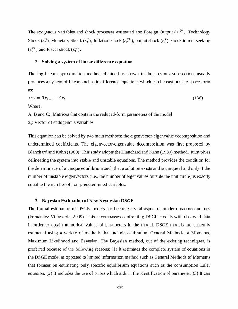
lxxix
The exogenous variables and shock processes estimated are: Foreign Output (εt𝑦𝑡
∗
), Technology
Shock (휀𝑡𝑎), Monetary Shock (휀𝑡
𝑟), Inflation shock (휀𝑡𝜋𝐷), output shock (휀𝑡
𝑦), shock to rent seeking
(휀𝑡𝑟𝑛) and Fiscal shock (휀𝑡
𝑔).
2. Solving a system of linear difference equation
The log-linear approximation method obtained as shown in the previous sub-section, usually
produces a system of linear stochastic difference equations which can be cast in state-space form
as:
𝐴𝑥𝑡 = 𝐵𝑥𝑡−1 + 𝐶𝑒𝑡 (138)
Where,
A, B and C: Matrices that contain the reduced-form parameters of the model
xt: Vector of endogenous variables
This equation can be solved by two main methods: the eigenvector-eigenvalue decomposition and
undetermined coefficients. The eigenvector-eigenvalue decomposition was first proposed by
Blanchard and Kahn (1980). This study adopts the Blanchard and Kahn (1980) method. It involves
delineating the system into stable and unstable equations. The method provides the condition for
the determinacy of a unique equilibrium such that a solution exists and is unique if and only if the
number of unstable eigenvectors (i.e., the number of eigenvalues outside the unit circle) is exactly
equal to the number of non-predetermined variables.
3. Bayesian Estimation of New Keynesian DSGE
The formal estimation of DSGE models has become a vital aspect of modern macroeconomics
(Fernández-Villaverde, 2009). This encompasses confronting DSGE models with observed data
in order to obtain numerical values of parameters in the model. DSGE models are currently
estimated using a variety of methods that include calibration, General Methods of Moments,
Maximum Likelihood and Bayesian. The Bayesian method, out of the existing techniques, is
preferred because of the following reasons: (1) It estimates the complete system of equations in
the DSGE model as opposed to limited information method such as General Methods of Moments
that focuses on estimating only specific equilibrium equations such as the consumption Euler
equation. (2) It includes the use of priors which aids in the identification of parameter. (3) It can
lxxx
address model misspecification by the inclusion of measurement errors in the system of equations
(4) It can also be used for model comparism (Grifolli, 2013).
The Bayesian method consists of using data 𝑌𝑇 to estimate the parameters 휃 of a model 𝑀. The
data 𝑌𝑇are observable values that are assumed to be given. The model 𝑀 hinges on economic
postulation and comprises of a vector of unobservable and random parameters; a likelihood
function, prior and posterior distribution. The likelihood function 𝑃(𝑌𝑇 |휃) is the probability the
model assigns to the data given the parameters. The prior 𝑃(휃) captures a researcher’s subjective
belief about the true value of the model’s parameters; while the posterior distribution shows the
state of knowledge of 휃 after each update. The link among the likelihood function, prior and
posterior distribution is summarised by Bayes’ Theorem. It shows that the posterior distribution is
proportional to the product of the likelihood function and priors
𝑃(휃|𝑌𝑇) =𝑃(𝑌𝑇|𝜃) 𝑃(𝜃)
𝑃(𝑌𝑇) (4.139)
𝑃(휃|𝑌𝑇) ∝ 𝑃(𝑌𝑇|휃) 𝑃(휃) = 𝐾(휃|𝑌∗) (4.140)
Where,
𝑃(휃|𝑌𝑇) : Posterior distribution
𝑃(𝑌𝑇|휃): Likelihood Function
𝑃(휃): Parameter Vector
𝑃(𝑌𝑇): Data
There are three main procedures for Bayesian estimation, these include: 1. calculate the log
likelihood function, 2. Specify Priors and 3. Simulate the posterior distribution
1. Calculate the log likelihood function
To obtain the log likelihood function, we start with the transition and the measurement equation.
The transition equation is the solution to the DSGE model, it shows that the paths of endogenous
variables in time t depends on predetermined variables and innovation. The measurement equation
on the other hand, links the DSGE model to data. The measurement equation shows that observable
data are explained by variables of the model and by some unobservable factors i.e; measurement
errors

lxxxi
Transition equation: 𝑌�� = 𝐷��𝑡−1+ 𝑒𝑡 (4.141)
Measurement equation: 𝑌𝑡∗ = 𝐹𝑌��+𝑢𝑡 (4.142)
Where 𝑢𝑡 and 𝑒𝑡 are innovation and assumed to be Gaussian white noise
processes:𝑢𝑡~𝑁𝐼𝐷 (0, 𝜎2);𝑒𝑡~𝑁𝐼𝐷 (0, 𝜎2)
If 𝑢𝑡 , 𝑒𝑡 and 𝑌0, the initial condition are normally distributed, then 𝑌�� and 𝑌𝑡∗ are also assumed to
be normally distributed. The next procedure entails using the Kalman filter to derive the log
likelihood function:
L=(𝑦∗|��∗) −𝑇𝑛
2log 2𝜋 −
1
2log | − Σ𝑦∗ | −
1
2(𝑦∗ − ��∗)′Σ𝑦∗
−1(𝑦∗ − ��∗) (4.143)
Where
𝑦∗: whole sample data;
n: number of observed variables;
T : number of periods in the sample;
��∗:expected value of 𝑦∗; and
Σ𝑦∗: variance-covariance matrix.
2. Specify Priors
In this stage, priors are specified for each parameter to be estimated. Priors give a pre-sample
description of the state of knowledge of the parameter vector, 휃. This allows the researcher to
incorporate extra information about the parameter vector 휃 based on their belief and which is not
captured by data 𝑌𝑇. The choice of priors depends on the category of the parameters to be
estimated. The categories of parameters include: a. parameters that affect the steady state of the
DSGE model such as the inflation rate, real interest rate and output growth rate; and b. parameters
that describe the law of motion of the exogenous shock process. Priors for steady state parameters
can be derived from pre-sample averages and existing empirical studies. Priors on shock processes
are also obtained from existing empirical studies.

lxxxii
The priors selected for each parameter are usually represented by probability distribution ranging
from normal, gamma and beta distributions. Prior distribution for parameters on the real line and
not- bonded are normal; for non-negative parameters could be gamma and log Normal; parameters
on a bounded interval take Beta distribution.
3. Simulate the Posterior Distribution
The posterior distribution is the probability assigned to the parameter value after observing the
data. It is an updating rule that relies on data to update a researcher’s prior belief about each model
parameter:
𝑃(휃|𝑌𝑇) =𝑃(𝑌𝑇|휃) 𝑃(휃)
𝑃(𝑌𝑇)
𝑃(휃|𝑌𝑇)is the posterior distribution.
𝑃(휃|𝑌𝑇) ∝ 𝑃(𝑌𝑇|휃) 𝑃(휃) = 𝐾(휃|𝑌∗)
Where 𝐾(휃|𝑌∗)is the posterior kernel
Take log of both sides:
log 𝐾(휃|𝑌∗) = log 𝑃(𝑌𝑇|휃) + log 𝑃(휃)
= log 𝑃(𝑌𝑇|휃) + 𝛿ℎ=1 log 𝑃(휃ℎ) (4.144)
Where h is the number of parameters to be estimated
Equation (4.144) is non-linear and difficult to estimate in an analytical manner. It then becomes
necessary to rely on a computational method. The Markov Chain Monte Carlo (MCMC) method
specifically the Metropolis Hastling is used to simulate the posterior distribution.
The Markov Chain Monte Carlo (MCMC) method is a simulation technique that is used to generate
samples from the posterior distribution based on the assumption that the samples drawn are
dependent. There are two major algorithm of the MCMC method: The Gibbs Sampling algorithm
and the Metropolis Hastings algorithm. The Metropolis Hastings algorithm is used in this study
since it is readily available in the Dynare software. The Metropolis Hastings algorithm is used to
draw samples from the posterior distribution that is unknown, that is, the researcher has limited
information about the distribution. This is unlike the Gibbs sampler that requires the knowledge

lxxxiii
of the full conditional distribution for relevant parameters to be computed. The Metropolis
Hastings algorithm involves the following procedures:
(1) Choose an initial arbitrary value 𝜽(𝟎)
(2) Draw candidate sample from the jumping distribution or proposal probability distribution
(3) Compute the acceptance ratio to determine whether to accept or reject a candidate sample
(4) Decide whether to accept or reject a candidate sample. The acceptance rate should be
between 0.25 and 0.33 (Grifolli, 2013).
(5) Repeat steps 2 to 4 N times, in order to draw N number of samples.
4.2.4 Data Sources and Measurements
This study obtained data over the period 1961Q1- 2016Q4 on six observable variables: output,
domestic inflation, government spending, terms of trade, and interest rate for the Nigerian
economy; and foreign output for the United States since it is chosen to be proxy for the world
economy. The domestic dataset for Nigeria was collected from the Statistical Bulletin of the
Central Bank of Nigeria; while the set of foreign data was sourced from the World Development
Indicators of the World Bank. The dataset for the study was transformed by applying the one-sided
Hodrick-Prescott filter to extract the cyclical components from its trend. This is required in order
to express the variables of the model as percentage deviation from their deterministic steady state
value. Due to the non-availability of quarterly data and its necessity for the short-run analysis
peculiar to DSGE models, the annual dataset was converted to quarterly series using the
interpolation method. In addition, the interpolation method proved useful in handling the few cases
of missing data. The dataset is presented in Table 4.4.

lxxxiv
Table 4.4: Data Description, Measurement and Sources
Variable Description/Measurement
Source
Real Gross Domestic
Product (Y)
Measures the value of goods produced in
the Nigerian economy. It is expressed in N’
Billion
CBN Stat. Bulletin
(2011, 2016)
Interest rate (R) Measures the lending rate adjusted for
inflation. It is expressed in percentage
World Development
Indicators (2016)
Govt. Expenditure (G) Captures the total spending of
the federal government in N’ Billion
CBN Stat. Bulletin
(2011, 2016)
Foreign GDP (Y*) It is the value of goods produced in the
economy of the United states (proxy for
world economy). It is expressed in $
Billion
World Development
Indicators (2016)
Terms of trade (S) It is calculated as the ratio of export to
imports.
CBN Stat. Bulletin
(2011, 2016)
Consumer Price Inflation This captures the domestic inflation rate in
the Nigerian economy. It is expressed in
percentage
CBN Stat. Bulletin
(2011, 2016)
4.3 Optimal Fiscal and Monetary Policy
The optimal fiscal and monetary policy is defined as the path of government spending and nominal
interest rates that optimise the objective function of the policy maker given the constraints posed
by the structural equations of the small open economy. There are three major methods to compute
the optimal policy. They include the optimal policy under commitment, that is, Ramsey Policy,
optimal policy under discretion and the optimal simple rule. In line with the objective of this study,
the Ramsey policy and optimal discretionary policy are chosen. This, specifically, allows one to
observe and compare the implication of rent seeking and discretion in describing the paths of the
optimal fiscal and monetary policy. The Ramsey Policy and Optimal policy under discretion are

lxxxv
computed in this section using the Linear Quadratic approximation to the objective function and
structural constraints. The calibration of the parameters is taken from Table 4.3.
4.3.1 Ramsey Policy
The problem of the Ramsey planner is to choose the interest rate and government spending
plans that minimise the welfare loss of the policy maker subject to the constraints of the small open
economy. The Ramsey plan is time-invariant, that is the planner chooses the paths of fiscal policy
and monetary policy instruments that it sticks with even at future dates (t+n). This makes the
Ramsey solution susceptible to the time-inconsistency problem The Ramsey policymaker,
therefore, seeks to minimise the deviation of the actual values of output, inflation and government
spending from their target values such that:
Min ∑ 𝜋2 + 0.5𝑦2 + 0.5𝑔2∞𝑡=0 (4.145)
Subject to the structural constraints that includes the open economy Dynamic IS curve, New
Keynesian Philips Curve and Fiscal Policy decision. These are of the form:
NK Philips Curve: 𝜋𝐷,𝑡 = βEt [𝜋𝐷,𝑡+1] + kα𝑦�� (4.134)
Where
kα = λ(𝜎𝛼 + 𝜑) =(1 − θ)(1 − βθ)
θ(𝜎𝛼 + 𝜑)
IS Curve:𝑦�� = 𝐸𝑡��𝑡+1 −1
𝜎𝛼(𝑟 − 𝐸𝑡Π𝐷,𝑡+1 − 𝑟𝑡
𝑛) (4.119)
Rent seeking government: 𝑔𝑡 =1
𝜁(𝑟𝑛𝑡) (4.99)
Benevolent Government: 𝑔𝑡 = 𝜌𝑔𝑔𝑡−1 + (1 − 𝜌𝑔)(𝜐𝑔𝑦) + 휀𝑡𝑔
(4.146)
4.3.2 Discretionary Policy
The discretionary policymaker is assumed to choose the path of interest rate and government
spending in every period t, based on the current state of the economy. This implies that the
discretionary policymaker re-optimises his objective function in every period t. The optimal policy
under discretion overcomes the time-inconsistency problem inherent in Ramsey policies.
lxxxvi
Furthermore, it mimics actual economic policy making in the real world than the Ramsey solution.
In this instance, the discretionary policymaker is concerned about minimising the per period loss
function subject to constraints in the economy such that:
Min 𝜋2 + 0.5𝑦2 + 0.5𝑔2 (4.147)
Subject to the structural constraints of the form:
NK Philips Curve: 𝜋𝐷,𝑡 = βEt [𝜋𝐷,𝑡+1] + kα𝑦�� (4.134)
Where
kα = λ(𝜎𝛼 + 𝜑) =(1 − θ)(1 − βθ)
θ(𝜎𝛼 + 𝜑)
IS Curve:𝑦�� = 𝐸𝑡��𝑡+1 −1
𝜎𝛼(𝑟 − 𝐸𝑡Π𝐷,𝑡+1 − 𝑟𝑡
𝑛) (4.119)
Rent seeking government: 𝑔𝑡 =1
𝜁(𝑟𝑛𝑡) (4.99)
Benevolent Government: 𝑔𝑡 = 𝜌𝑔𝑔𝑡−1 + (1 − 𝜌𝑔)(𝜐𝑔𝑦) + 휀𝑡𝑔
(4.146)

lxxxvii
CHAPTER FIVE
RESULTS AND DISCUSSION
This chapter empirically addresses the three objectives of this study. The first objective analyses
the empirical nature of the interactions between fiscal and monetary policies. The second objective
is to examine the transmission effects of the policy interactions on macroeconomic variables such
as inflation and output. Finally, the third objective considers the optimal combination of fiscal and
monetary policy. The Chapter is divided into five sections. The estimation results of this study are
presented in section 5.1. Model diagnostic testing on the estimated model is conducted in Section
5.2. In Sections 5.3 and 5.4, the results on the nature of fiscal and monetary policy interactions
and the optimal paths of fiscal and monetary policy are presented. Finally, in Section 5.5, the main
findings of this study are highlighted.
5.1 Presentation of Results
The results of Bayesian estimation, Impulse Response Functions and Variance Decomposition are
presented in this Section. These outputs are obtained by using Dynare Version 4.5.1 on Octave
4.2.1 to run the relevant codes. The Dynare package is a pre-processor that runs on both Matlab
and Octave and are used to solve and estimate Dynamic Stochastic General Equilibrium Models
(Grifolli, 2013). Specifically, the Bayesian technique is used to estimate parameters from the
system of equations of the New Keynesian DSGE model outlined in Chapter 4. The estimation
process includes the following steps: (1) obtain the reduced form solution of the DSGE model (2)
derive a state-space representation of the model which maps unobserved state variables into the
observed data (3) the likelihood function of the observed data is got by applying the Kalman filter
to the reduced form (4) Monte-Carlo based optimisation of the posterior kernel to obtain the
posterior mode (5) a Metropolis-Hastings algorithm is used to generate 100,000 draws of 5 chains
from the posterior distribution, in order to compute the posterior moments. Out of the 100, 000
draws, 30,000 draws were discarded in order to ensure convergence.

lxxxviii
5.1.1 Parameter Estimates of the DSGE Model
A. Structural Parameter
Table 5.1 present the estimates of the structural parameters. It shows the posterior mean of each
estimated parameter alongside their prior mean. The posterior estimate of habit formation is 0.86
and is higher than its prior mean. This implies that a large share of Nigerian households slowly
changes their consumption pattern following an income shock. It depicts the tendency of Nigerian
households to base their current preferences on past consumption patterns. For instance, several
Nigerians are likely to resort to borrowing, so as to retain their lifestyle and taste, despite the fall
in their real wages. The posterior mean of habit formation is lower when compared with the
estimate found by Mordi et al., (2013) at 0.94.
The inverse elasticity of inter-temporal substitution,(σ), shows the magnitude by which
consumption is sensitive to changes in the interest rate. The posterior mean of the inverse elasticity
of inter-temporal substitution is estimated to be 1.82. The elasticity of intertemporal substitution,
on the other hand, is, therefore, calculated to be 0.55. It can then be interpreted that consumption
is insensitive to changes in the real interest rate in Nigeria. Increases in the real interest rate, in this
instance, is not expected to induce consumers to forego current consumption for the future. This
is evident in the poor saving culture among several Nigerians who prefer to spend in the present
than save for the future. An exception to Nigerians' poor saving attitude is the retirement savings
scheme which several Nigerian workers have been institutionally compelled to subscribe to. The
retirement scheme encourages these individuals to forego present spending for future benefits. The
posterior estimate of the inverse elasticity of inter-temporal substitution is clearly distinct from its
prior mean at 3.00 and at the same time, it is lower than the estimated value in Cebi (2011).
The estimated value of the share of non-Ricardian households,(𝜓), at 0.703 is clearly higher than
the reported estimate of 0.37 in Muscatelli, Tirelli and Trecroci (2005). The difference in the
estimate of the parameter lies in the distinct economic structure between the advanced economy
of the United States and the developing one of Nigeria. The result depicts the presence of a large
share of liquidity constrained individuals, that is, non-Ricardian households in Nigeria. These
individuals live from hand to mouth, this means that they only consume but cannot save. In
Nigeria, there is a higher propensity to consume than to save. This is because many Nigerians

lxxxix
spend a greater proportion of their income on food, shelter and energy, with little of their income
left for savings. Statistics reveal that Nigeria spends about 65 percent of its total expenditure on
food alone (National Bureau of Statistics, 2012).
The posterior mean of Calvo price stickiness, (휃), at 0.499 is slightly lower than its prior mean.
This differs from the finding of Rasaki (2017) who estimated the price stickiness parameter to be
0.71. The estimated value of Calvo price stickiness at 0.499 shows that about 50 percent of firms,
do not re-optimise their prices in a given quarter. It also implies that price contracts remain fixed
for about two quarters. This implies that businesses and firms in Nigeria tend to change the prices
of their goods and services every six months. The frequent change in the prices of goods and
services is suspected to originate from fluctuations in the prices of food and exchange rates, in the
Nigerian economy.
Furthermore, the parameter estimate of the degree of openness, 𝛼, is higher than its prior mean. It
shows that Nigeria has a high degree of openness to trade. Foreign trade is therefore believed to
wield a good influence on the domestic economy of Nigeria. For instance, Nigeria has gained
tremendously from its exports of primary products such as agricultural produce and crude oil. At
the same time, imports of raw materials, manufactured goods, electronics and cars have been able
to improve living conditions in the country. The posterior mean for the elasticity of substitution
between home and foreign goods, (휂), is positive and high, such that, Nigerians are perceived to be
willing to forego their consumption of local products in preference for imported goods. It shows
that consumers’ preference for imported goods is high. On average, Nigerians prefer to consume
imported clothes, shoes, electronics. This is suspected to be linked to the poor quality and lack of
competitiveness of their locally made counterparts. This has, therefore, necessitated recent
campaigns for ‘made in Nigeria’ products.
The posterior estimate of the inverse elasticity of labour, 𝜑, is found to be greater than its prior
mean. The inverse elasticity of labour shows the responsiveness of labour supply to changes in the
wage rate. The elasticity of labour is low at 0.22 (this is calculated as 1/4.5). This depicts that the
amount of labour supplied by Nigerian workers can be insensitive to changes in the wage rate. For
instance, in spite of cuts in their salaries, many Nigerian workers consider the dire state of
unemployment in the country and are less likely to quit their jobs.
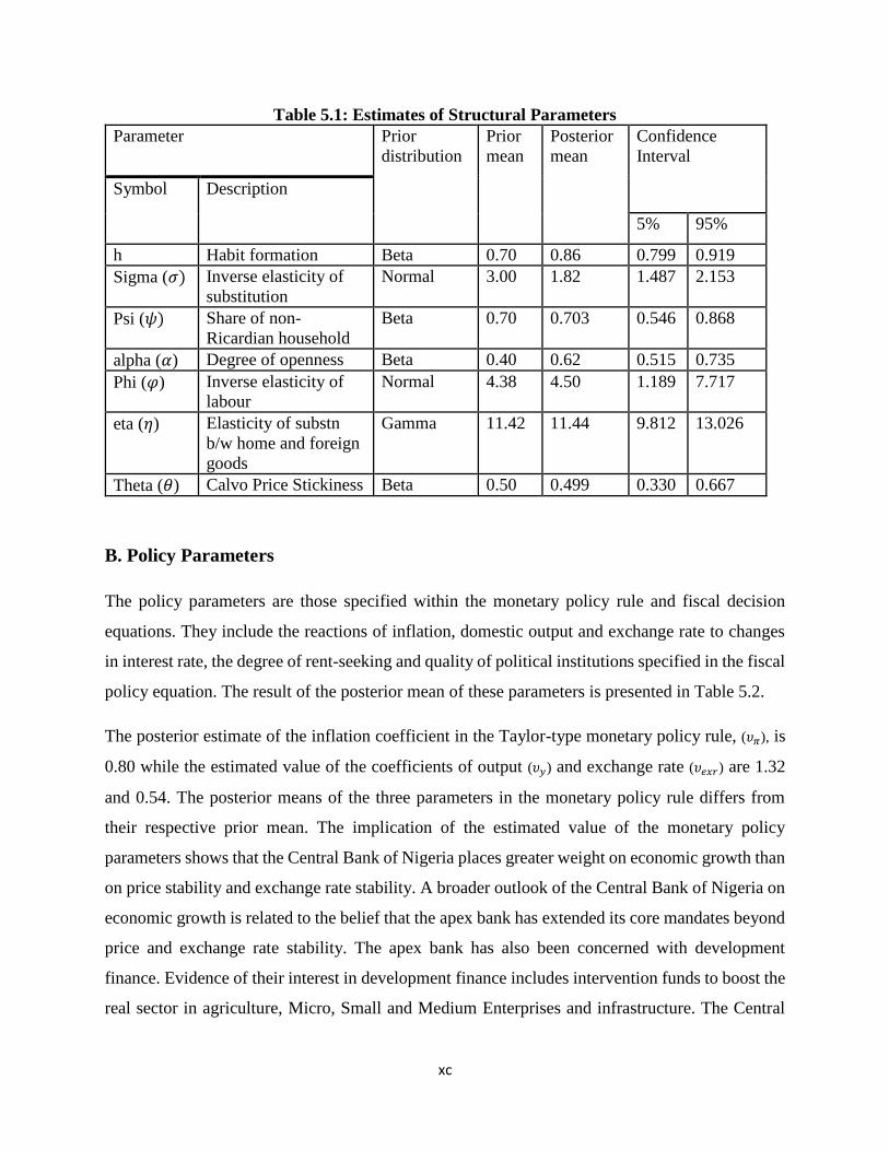
xc
Table 5.1: Estimates of Structural Parameters
Parameter Prior
distribution
Prior
mean
Posterior
mean
Confidence
Interval
Symbol Description
5% 95%
h Habit formation Beta 0.70 0.86 0.799 0.919
Sigma (𝜎) Inverse elasticity of
substitution
Normal 3.00 1.82 1.487 2.153
Psi (𝜓) Share of non-
Ricardian household
Beta 0.70 0.703 0.546 0.868
alpha (𝛼) Degree of openness Beta 0.40 0.62 0.515 0.735
Phi (𝜑) Inverse elasticity of
labour
Normal 4.38 4.50 1.189 7.717
eta (휂) Elasticity of substn
b/w home and foreign
goods
Gamma 11.42 11.44 9.812 13.026
Theta (휃) Calvo Price Stickiness Beta 0.50 0.499 0.330 0.667
B. Policy Parameters
The policy parameters are those specified within the monetary policy rule and fiscal decision
equations. They include the reactions of inflation, domestic output and exchange rate to changes
in interest rate, the degree of rent-seeking and quality of political institutions specified in the fiscal
policy equation. The result of the posterior mean of these parameters is presented in Table 5.2.
The posterior estimate of the inflation coefficient in the Taylor-type monetary policy rule, (𝜐𝜋), is
0.80 while the estimated value of the coefficients of output (𝜐𝑦) and exchange rate (𝜐𝑒𝑥𝑟) are 1.32
and 0.54. The posterior means of the three parameters in the monetary policy rule differs from
their respective prior mean. The implication of the estimated value of the monetary policy
parameters shows that the Central Bank of Nigeria places greater weight on economic growth than
on price stability and exchange rate stability. A broader outlook of the Central Bank of Nigeria on
economic growth is related to the belief that the apex bank has extended its core mandates beyond
price and exchange rate stability. The apex bank has also been concerned with development
finance. Evidence of their interest in development finance includes intervention funds to boost the
real sector in agriculture, Micro, Small and Medium Enterprises and infrastructure. The Central
xci
Bank of Nigeria also provided bailout funds to support states that experienced difficulty in
payment of workers' salaries. Adebiyi and Mordi (2016) on the contrary, find that the Central Bank
of Nigeria is primarily concerned with price stability. Another implication of the coefficient of
Taylor rule reaction to inflation is interpreted in the sense of Leeper (1991). Monetary policy is
active (passive) when the estimated value of the Taylor reaction to inflation, is greater (less) than
one. The result observed from Table 5.2 shows that monetary policy took a passive stance over the
sample period. Furthermore, the posterior value of the degree of interest rate smoothing (𝜌𝑟) shows
that the lagged interest rate plays a significant role in determining the current interest rate.
The posterior mean of the proxy for rent-seeking (𝝌) is estimated to be 0.21, which shows that
only 21 percent of government revenue is generated for public spending, the remaining 79 percent
are suspected to be wasted or misused for corrupt and self-interested activities spending. For
instance, the Minister of Information, Lai Mohammed, commented that one third of the public
funds stolen by former politicians and bureaucrats between 2006 and 2013, could have provided
635.18 kilometres of road; built one ultra-modern hospital in each state of the Federation; erected
183 schools; educated 3,974 children from primary school to University; and provided 20,062
units of 2-bedroom houses, in order to ease accommodation. On the other hand, the posterior
estimate of the quality of political institutions (𝜻) suggests, rather puzzlingly, the existence of
strong political institutions in Nigeria.

xcii
Table 5.2: Estimates of Policy Parameters
Parameter Prior
distribution
Prior
mean
Posterior
mean
Confidence
Interval
Symbol Description
5% 95%
upsillon_pii
(𝜐𝜋)
Taylor feedback on
Inflation
Gamma 1.50 0.80 0.686 0.918
upsillon_y
(𝜐𝑦)
Taylor feedback on
Output
Gamma 0.50 1.32 1.209 1.418
upsillon_exr
(𝜐𝑒)
Taylor feedback on
exchange rate
Gamma 0.80 0.54 0.451 0.634
rrho_r (𝜌𝑟) Interest rate
smoothening
Beta 0.70 0.86 0.840 0.889
cchi (𝜒) Degree of rent- seeking Beta 0.50 0.21 0.126 0.277
Zetta (휁) Quality of political
institutions
Beta 0.35 0.79 0.716 0.862
C. Persistent Parameters
Persistent parameters are coefficients of the lagged dependent variable in the autoregressive
equations of order one, AR(1). The parameter values are expected to range between zero and one,
such that the value at zero and one are interpreted respectively as non-persistence and persistent
parameters. The degree of persistence of a parameter shows how long it takes for an economy to
return to steady state after a perturbation. Parameters with a high persistence value (close to one)
mean that the economy slowly adjusts to unexpected shocks, and, conversely for parameters with
lower persistence values, the economy quickly returns to steady after an unexpected shock.
The results on the estimates of the persistent parameters as reported in Table 5.3, shows that all
the parameters of the AR(1) process are highly persistent. Furthermore, the posterior mean of the
individual persistent parameters is higher than their prior mean. An implication of this finding is
that it takes a prolonged time for the Nigerian economy to adjust to the shocks listed in Table 5.3.
Therefore, when macroeconomic policies are implemented, the Nigerian economy adjusts slowly
to it. Adegboye (2015) also finds persistent but lower values for some of the AR(1) coefficients.

xciii
Table 5.3: Estimates of Persistent Parameters
Parameter Prior
distribution
Prior
mean
Posterior
mean
Confidence
Interval
Symbol Description 5% 95%
rrho_ystar
(𝜌𝑦𝑠𝑡𝑎𝑟)
AR(1) of foreign
output
Beta 0.70 0.92 0.881 0.962
rrho_a
(𝜌𝑎)
AR(1) of technology Beta 0.70 0.702 0.548 0.865
rrho_piiD
(𝜌𝑝𝑖𝑖𝐷)
AR(1) of inflation
shock
Beta 0.70 0.701 0.543 0.867
rrho_sr
(𝜌𝑠𝑟)
AR(1) of interest
rate shock
Beta 0.70 0.90 0.864 0.941
rrho_sg
(𝜌𝑠𝑔)
AR(1) of
government
spending shock
Beta 0.70 0.98 0.968 0.991
rrho_sy
(𝜌𝑠𝑦)
AR(1) of output
shock
Beta 0.70 0.93 0.900 0.954
rrho_srn
(𝜌𝑠𝑟𝑛)
AR(1) of shock to
rent-seeking
Beta 0.70 0.80 0.763 0.840
D. Shock Parameters
Table 5.4 present the posterior estimates of the shock parameters. The size of these parameters
provides a measure of the volatility of individual shocks. Table 5.4 shows that output shocks is the
most volatile, with a posterior mean of 0.68. The next volatile ones are the inflation and technology
shocks with posterior estimates of 0.28 and 0.23, respectively. The least volatile shocks are those
of government spending, interest rate, foreign output and rent-seeking with estimated means of
0.07, 0.04, 0.03 and 0.03. It can then be deduced that output shock is the most volatile, that is, the
most significant source of economic fluctuations to the Nigerian economy. On the other hand,
shocks to rent seeking and foreign output, are found to be the least volatile.
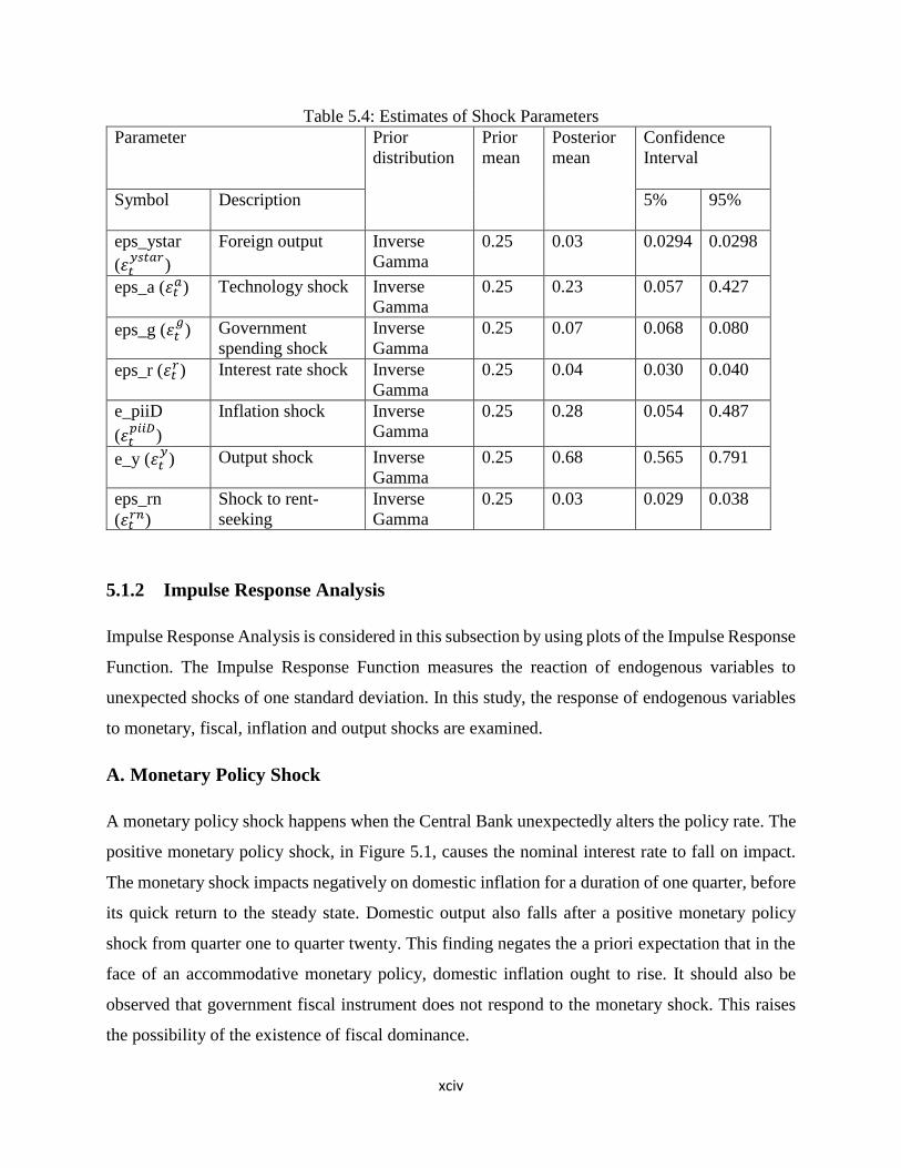
xciv
Table 5.4: Estimates of Shock Parameters
Parameter Prior
distribution
Prior
mean
Posterior
mean
Confidence
Interval
Symbol Description
5% 95%
eps_ystar
(휀𝑡𝑦𝑠𝑡𝑎𝑟
)
Foreign output Inverse
Gamma
0.25 0.03 0.0294 0.0298
eps_a (휀𝑡𝑎) Technology shock Inverse
Gamma
0.25 0.23 0.057 0.427
eps_g (휀𝑡𝑔
) Government
spending shock
Inverse
Gamma
0.25 0.07 0.068 0.080
eps_r (휀𝑡𝑟) Interest rate shock Inverse
Gamma
0.25 0.04 0.030 0.040
e_piiD
(휀𝑡𝑝𝑖𝑖𝐷
)
Inflation shock Inverse
Gamma
0.25 0.28 0.054 0.487
e_y (휀𝑡𝑦
) Output shock Inverse
Gamma
0.25 0.68 0.565 0.791
eps_rn
(휀𝑡𝑟𝑛)
Shock to rent-
seeking
Inverse
Gamma
0.25 0.03 0.029 0.038
5.1.2 Impulse Response Analysis
Impulse Response Analysis is considered in this subsection by using plots of the Impulse Response
Function. The Impulse Response Function measures the reaction of endogenous variables to
unexpected shocks of one standard deviation. In this study, the response of endogenous variables
to monetary, fiscal, inflation and output shocks are examined.
A. Monetary Policy Shock
A monetary policy shock happens when the Central Bank unexpectedly alters the policy rate. The
positive monetary policy shock, in Figure 5.1, causes the nominal interest rate to fall on impact.
The monetary shock impacts negatively on domestic inflation for a duration of one quarter, before
its quick return to the steady state. Domestic output also falls after a positive monetary policy
shock from quarter one to quarter twenty. This finding negates the a priori expectation that in the
face of an accommodative monetary policy, domestic inflation ought to rise. It should also be
observed that government fiscal instrument does not respond to the monetary shock. This raises
the possibility of the existence of fiscal dominance.
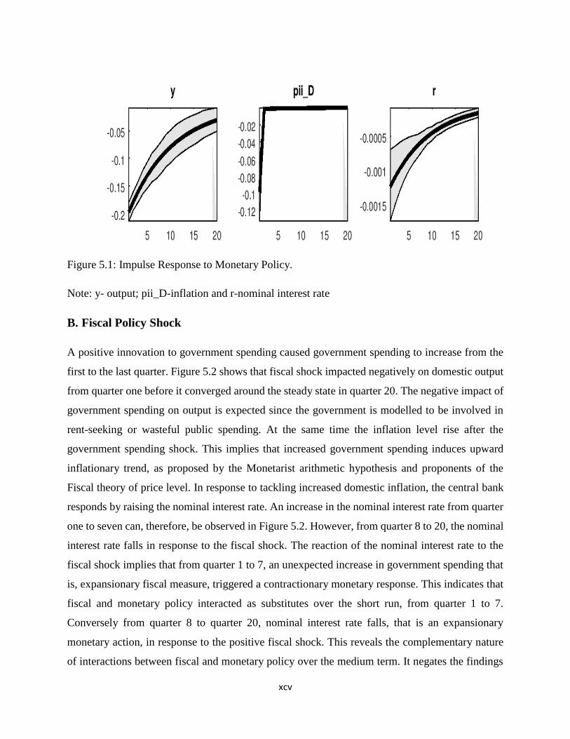
xcv
Figure 5.1: Impulse Response to Monetary Policy.
Note: y- output; pii_D-inflation and r-nominal interest rate
B. Fiscal Policy Shock
A positive innovation to government spending caused government spending to increase from the
first to the last quarter. Figure 5.2 shows that fiscal shock impacted negatively on domestic output
from quarter one before it converged around the steady state in quarter 20. The negative impact of
government spending on output is expected since the government is modelled to be involved in
rent-seeking or wasteful public spending. At the same time the inflation level rise after the
government spending shock. This implies that increased government spending induces upward
inflationary trend, as proposed by the Monetarist arithmetic hypothesis and proponents of the
Fiscal theory of price level. In response to tackling increased domestic inflation, the central bank
responds by raising the nominal interest rate. An increase in the nominal interest rate from quarter
one to seven can, therefore, be observed in Figure 5.2. However, from quarter 8 to 20, the nominal
interest rate falls in response to the fiscal shock. The reaction of the nominal interest rate to the
fiscal shock implies that from quarter 1 to 7, an unexpected increase in government spending that
is, expansionary fiscal measure, triggered a contractionary monetary response. This indicates that
fiscal and monetary policy interacted as substitutes over the short run, from quarter 1 to 7.
Conversely from quarter 8 to quarter 20, nominal interest rate falls, that is an expansionary
monetary action, in response to the positive fiscal shock. This reveals the complementary nature
of interactions between fiscal and monetary policy over the medium term. It negates the findings

xcvi
of Adegboye (2015) that fiscal and monetary policy acts as complements in the short term and act
as substitutes in the medium term.
Figure 5.2: Impulse Response to Fiscal Policy Shock
Note: y- output; pii_D-inflation; r-nominal interest rate and g-government spending
C. Output Shock
From Figure 5.3, a positive output shock monotonically increased the level of domestic output into
the horizon but reduced the price level and nominal interest rate. The reaction of the price level is
expected because a rise in the level of output implies an increased production of goods and lower
unemployment level, which means that household are earning an adequate income to demand
goods and at the same time, aggregate supply is increasing, this will prevent demand-pull inflation.
The reduction of the price level after an output shock is also intuitively backed by the Philip’s
curve which depicts a trade-off between output and inflation. In addition, the Central Bank reduces
the interest rate in response to positive output shock, in order to sustain the rising output level.

xcvii
Figure 5.3: Impulse Response to Output Shock
Note: y- output; pii_D-inflation and r-nominal interest rate
D. Shock to Rent seeking
Shock to rent-seeking implies an increase in the amount of rent raised. A sudden rise in the amount
of wasteful spending or amount of rent raised, as seen in Figure 5.4, impacted negatively on
domestic output, over a period of three quarters by 0.12 percentage points before its return to the
steady state level. This shows that rent-seeking activities have an initial adverse impact on
domestic output. It shows that rent-seeking activities impact negatively on the Nigerian economy
but the economy quickly adjusts to it. This means that the money being stolen and misused by
public office holders negatively impacts the Nigerian economy.

xcviii
Figure 5.4: Impulse Response of Shock to Rent-Seeking
Note: y- output; pii_D-inflation; r-nominal interest rate; rn-rent seeking; g-government spending
5.1.3 Variance Decomposition
The variance decomposition method considers the relative contribution of individual shocks to
fluctuations in an endogenous variable. The variance decomposition presents the percentage of
variance of the error that arises from the shock of the variable due to itself and other variables over
a specific time horizon. It is useful in measuring the importance of a shock as a source of volatility
to a macroeconomic variable. The variance decomposition of output, inflation, interest rate, rent-
seeking and government spending are examined in this sub-section.
From Table 5.7, it can be observed that interest rate and foreign output shocks contribute most to
variations in output at 58.86 percent and 28.99 percent, respectively. Shocks to foreign inflation,
foreign interest rate, tax, rent-seeking and output itself, also respectively accounted for fluctuations
in domestic output at 3.91, 2.66, 0.78, 4.72, 0.01 percent. Conversely, technology shock, transfer

xcix
payment shock and inflation shock did not trigger any variation in domestic output. It is also
observed that external shocks, that is, foreign inflation, foreign interest rate and foreign output are
the main sources of volatility in domestic inflation at 16.82, 36.84 and 38.77 percent. On the other
hand, domestic sources of shocks such as government spending, interest rate, tax, output and rent-
seeking accounted for lesser variations in domestic inflation at 0.05, 0.14, 0.54, 1.19, 5.65 percent,
respectively.
The result of the variance decomposition also reveals that foreign inflation and foreign interest rate
are the main perturbations to the domestic interest rate. They contributed 29.07 and 61.95 percent
to variations in the nominal interest rate. Other sources of shocks such as government spending,
interest rate, foreign output, tax, output and rent-seeking account for 1.31, 0.13, 1.49, 0.82, 1.06
and 4.16 percent volatility in the nominal interest rate. Domestic shocks, that is, government
spending shocks and shocks to rent-seeking are the only contributor to the variations in
government spending at 92.23 and 7.09 percent. The other form of shocks does not trigger
fluctuations in government spending. At the same time, the volatility in rent-seeking is primarily
explained by shocks to rent-seeking itself and tax revenue at 91.34 and 8.66 percent. The result
reveals the importance of both foreign and domestic shocks to fluctuations in the Nigerian
economy.

c
Table 5.7: Posterior mean variance decomposition (percent)
Model Diagnostic Testing
The estimated model is a small-scale New Keynesian DSGE model with a system of 27 equations
and 27 endogenous variables. The posterior moments of this model are computed by using the
Metropolis-Hastings algorithm where 100,000 posterior draws of 5 parallel chains are generated,
after the first 30,000 draws are discarded, in order to ensure convergence. In addition, the Monte-
Carlo based optimisation method is used to obtain the posterior mode. In this Section, therefore,
the statistical validity of the estimated model is examined. This involves presenting graphs on the
numerical optimisation of the posterior kernel and the Metropolis-Hastings algorithm, in order to
detect problems or build confidence in the results of the estimated model.
5.2.1 Stability of the Model
This is about the existence and uniqueness of a solution to the adopted NK DSGE model. A
solution exists when the number of equations equals the number of endogenous variables. In the
case of this study, this condition is met such that there are 27 equations with 27 endogenous
variables. The Blanchard-Kahn condition is also used to test for the existence of a unique solution
to this model. The condition requires that the number of eigenvectors lying outside a unit root
equals the number of forward-looking variables. The Blanchard-Kahn condition of the estimated
Output Domestic
Inflation
Nominal
Interest
rate
Government
spending
Rent
Seeking
Govt. Spending shock (eps_g)
Interest Rate shock (eps_r)
Foreign Output (eps_ystar)
Foreign Inflation (eps_piistar)
Foreign Interest rate
(eps_rstar)
Technology Shock (eps_a)
Tax Shock (eps_taxx)
Transfer payment shock
(eps_TP)
Inflation shock (e_piiD)
Output shock (e_y)
Shock to Rent seeking
(eps_rn)
0.06
58.8
28.99
3.91
2.66
0.00
0.78
0.00
0.00
0.01
4.72
0.05
0.14
38.77
16.82
36.84
0.00
0.54
0.00
0.00
1.19
5.65
1.31
0.13
1.49
29.07
61.95
0.00
0.82
0.00
0.00
1.06
4.16
92.23
0.00
0.00
0.00
0.00
0.00
0.68
0.00
0.00
0.00
7.09
0.00
0.00
0.00
0.00
0.00
0.00
8.66
0.00
0.00
0.00
91.34
ci
model is satisfied such that there are three eigenvalues larger than one in modulus as there are
three forward-looking variables in the system. This depicts the existence of a unique solution for
the estimated system of equations.
5.2.2 Identification of the Parameter Estimates
The estimated parameters of the model are expected to be identified by the observed data. This
means that the observed data provide sufficient information about the parameters. The criterion
used to gauge parameter identification is the distinctness between the prior and posterior
distribution such that they are not the same. Identical prior and posterior distributions imply that
the concerned parameter is only weakly identified and the data is uninformative. It can also mean
in a converse manner that the data provides perfectly accurate information about the parameter.
Tables 5.1 to 5.4 show that the prior values are different from the posterior values for most of the
estimated parameters. This is also corroborated by the plots presented in Figures 5.5a, 5.5b and in
Appendix nine, which shows that the prior distribution (grey line) is distinct from the posterior
distribution (black line) for most of the parameters.
Furthermore, the plots of posterior distribution (black curve) possess a near normal shape while,
at the same time, the mode computed from the numerical optimization of the posterior kernel
(green vertical line) is seen to be close to the peak of the posterior distribution (black curve). These
two additional features justify further confidence in the output of the estimated model.

cii
Figure 5.5a: Prior-Posterior Plots

ciii
Figure 5.5b: Prior-Posterior Plots
5.2.3 Mode Check
The accuracy of the Monte-Carlo based optimisation routine used in computing the posterior mode
is inspected using the mode check plots. The computed mode (green line) should ideally be located
at the maximum of the posterior likelihood (blue line) for each parameter. There are possible
problems with the optimization routine if this is not the case. The mode plots presented in Figure
5.6 show that the estimated mode (green line) is close to the maximum of the posterior likelihood
(blue line). The implication is that the optimiser was able to compute a robust maximum for the
posterior mode. The deviations between the red line (posterior mode) and the blue line (likelihood
function) depict the influence of the prior on the likelihood function (blue line).
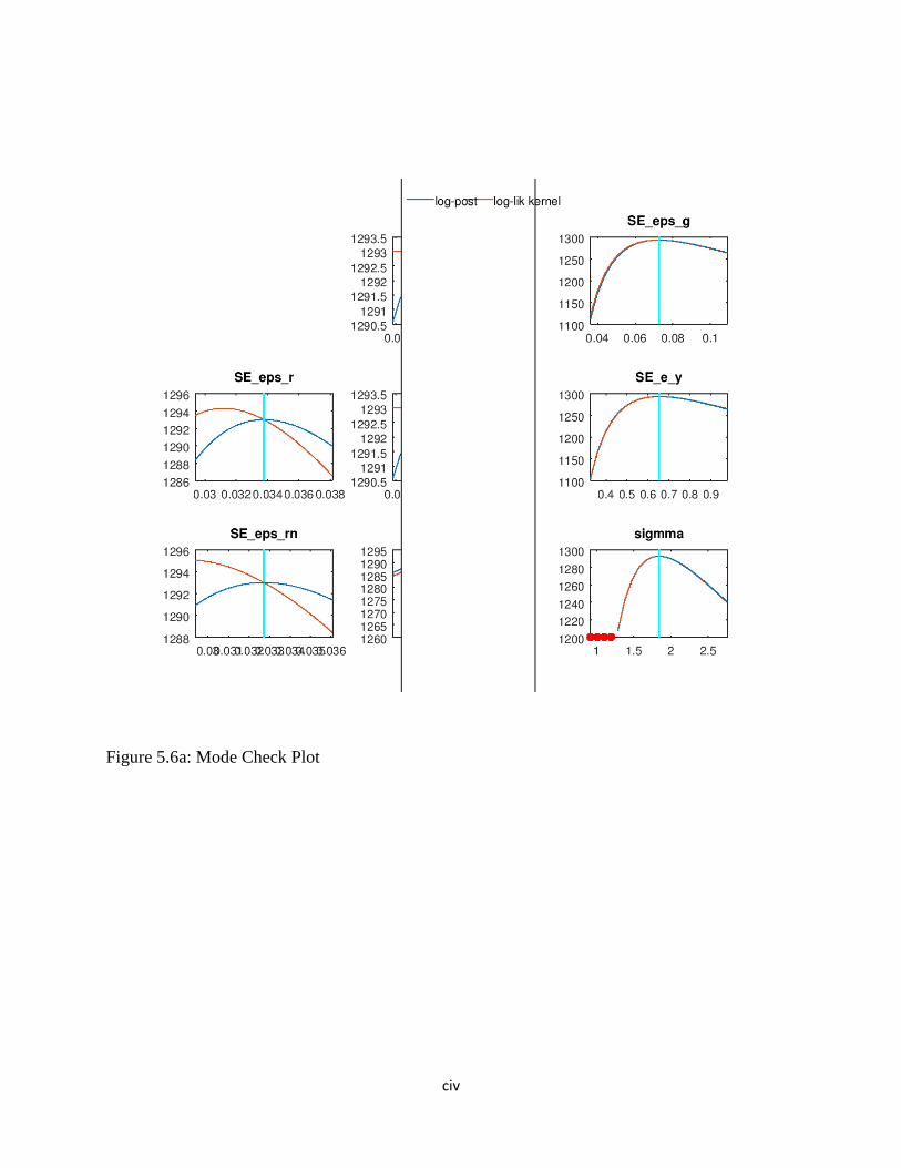
civ
Figure 5.6a: Mode Check Plot
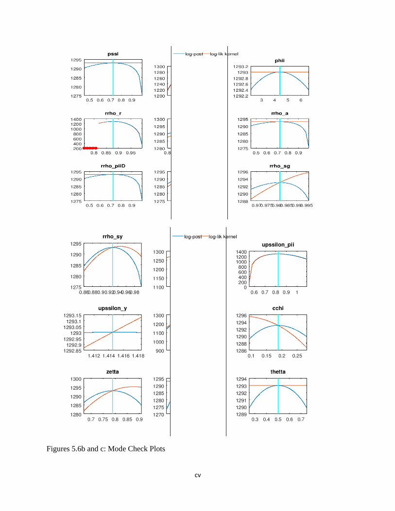
cv
Figures 5.6b and c: Mode Check Plots
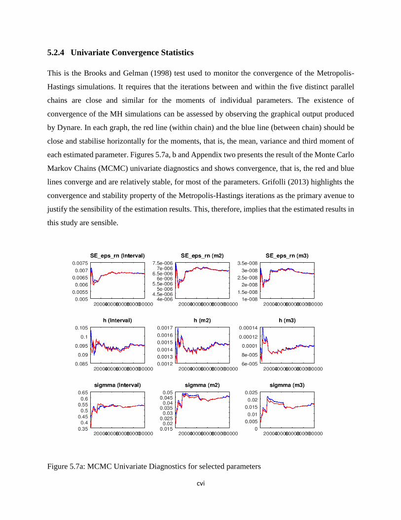
cvi
5.2.4 Univariate Convergence Statistics
This is the Brooks and Gelman (1998) test used to monitor the convergence of the Metropolis-
Hastings simulations. It requires that the iterations between and within the five distinct parallel
chains are close and similar for the moments of individual parameters. The existence of
convergence of the MH simulations can be assessed by observing the graphical output produced
by Dynare. In each graph, the red line (within chain) and the blue line (between chain) should be
close and stabilise horizontally for the moments, that is, the mean, variance and third moment of
each estimated parameter. Figures 5.7a, b and Appendix two presents the result of the Monte Carlo
Markov Chains (MCMC) univariate diagnostics and shows convergence, that is, the red and blue
lines converge and are relatively stable, for most of the parameters. Grifolli (2013) highlights the
convergence and stability property of the Metropolis-Hastings iterations as the primary avenue to
justify the sensibility of the estimation results. This, therefore, implies that the estimated results in
this study are sensible.
Figure 5.7a: MCMC Univariate Diagnostics for selected parameters
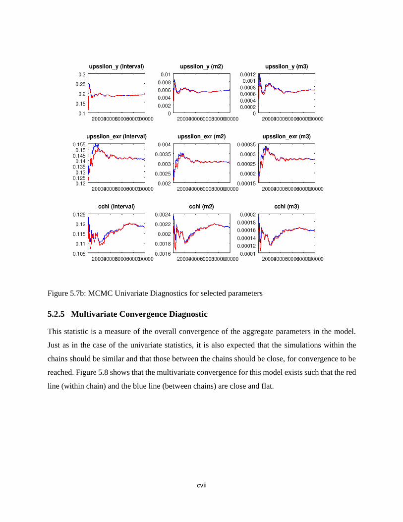
cvii
Figure 5.7b: MCMC Univariate Diagnostics for selected parameters
5.2.5 Multivariate Convergence Diagnostic
This statistic is a measure of the overall convergence of the aggregate parameters in the model.
Just as in the case of the univariate statistics, it is also expected that the simulations within the
chains should be similar and that those between the chains should be close, for convergence to be
reached. Figure 5.8 shows that the multivariate convergence for this model exists such that the red
line (within chain) and the blue line (between chains) are close and flat.
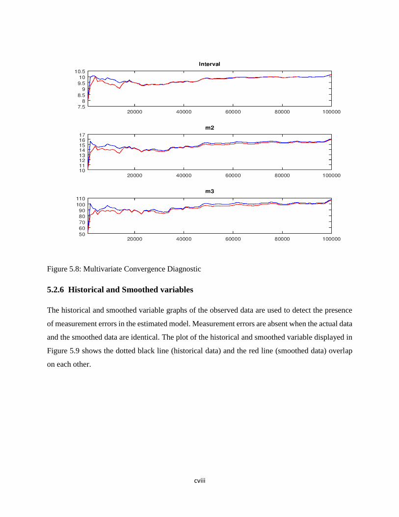
cviii
Figure 5.8: Multivariate Convergence Diagnostic
5.2.6 Historical and Smoothed variables
The historical and smoothed variable graphs of the observed data are used to detect the presence
of measurement errors in the estimated model. Measurement errors are absent when the actual data
and the smoothed data are identical. The plot of the historical and smoothed variable displayed in
Figure 5.9 shows the dotted black line (historical data) and the red line (smoothed data) overlap
on each other.

cix
Figure 5.9: Historical and Smoothed variables
5.2.7 Smoothed Shocks
The plot of the smoothed estimated shocks is expected to centre around zero. Figure 5.10 shows
that the smoothed shocks processes are around zero. This is an indication of the statistical validity
of the estimated model.
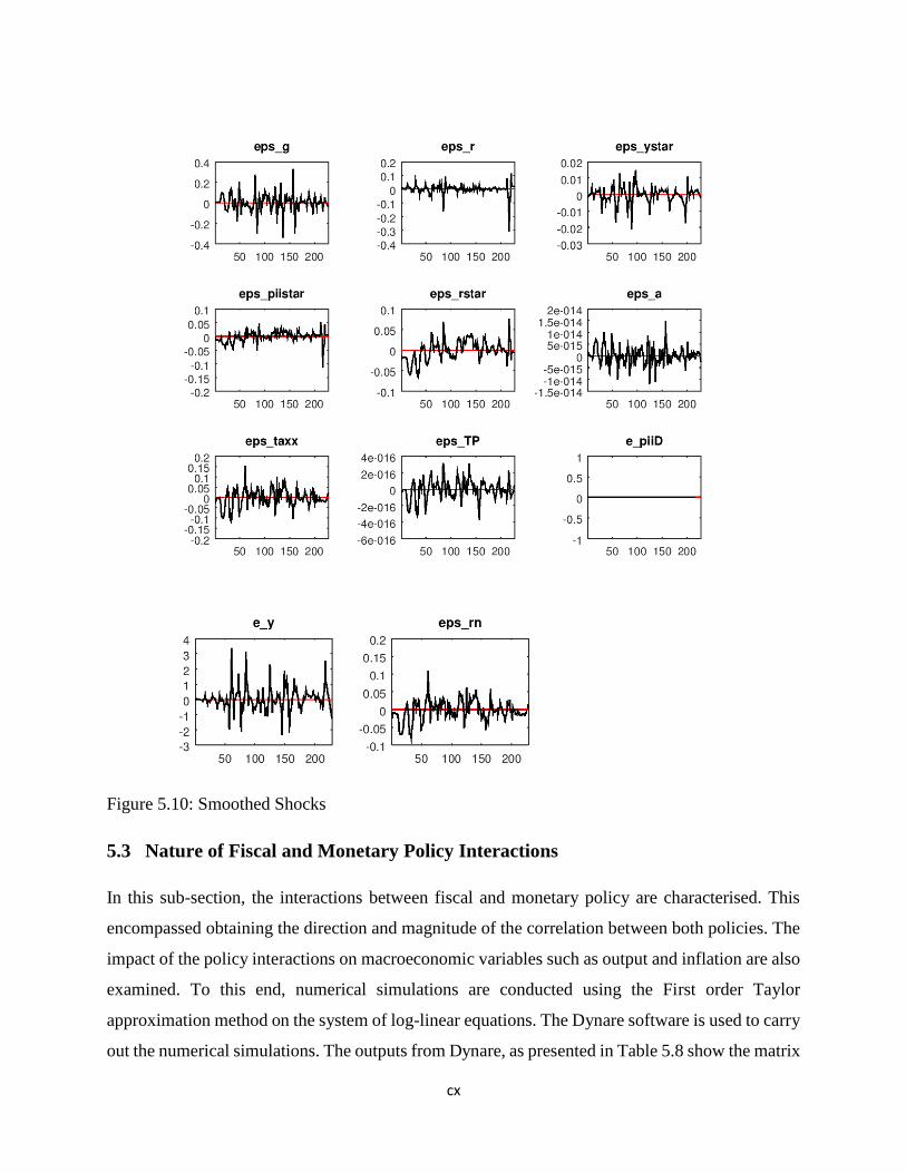
cx
Figure 5.10: Smoothed Shocks
5.3 Nature of Fiscal and Monetary Policy Interactions
In this sub-section, the interactions between fiscal and monetary policy are characterised. This
encompassed obtaining the direction and magnitude of the correlation between both policies. The
impact of the policy interactions on macroeconomic variables such as output and inflation are also
examined. To this end, numerical simulations are conducted using the First order Taylor
approximation method on the system of log-linear equations. The Dynare software is used to carry
out the numerical simulations. The outputs from Dynare, as presented in Table 5.8 show the matrix
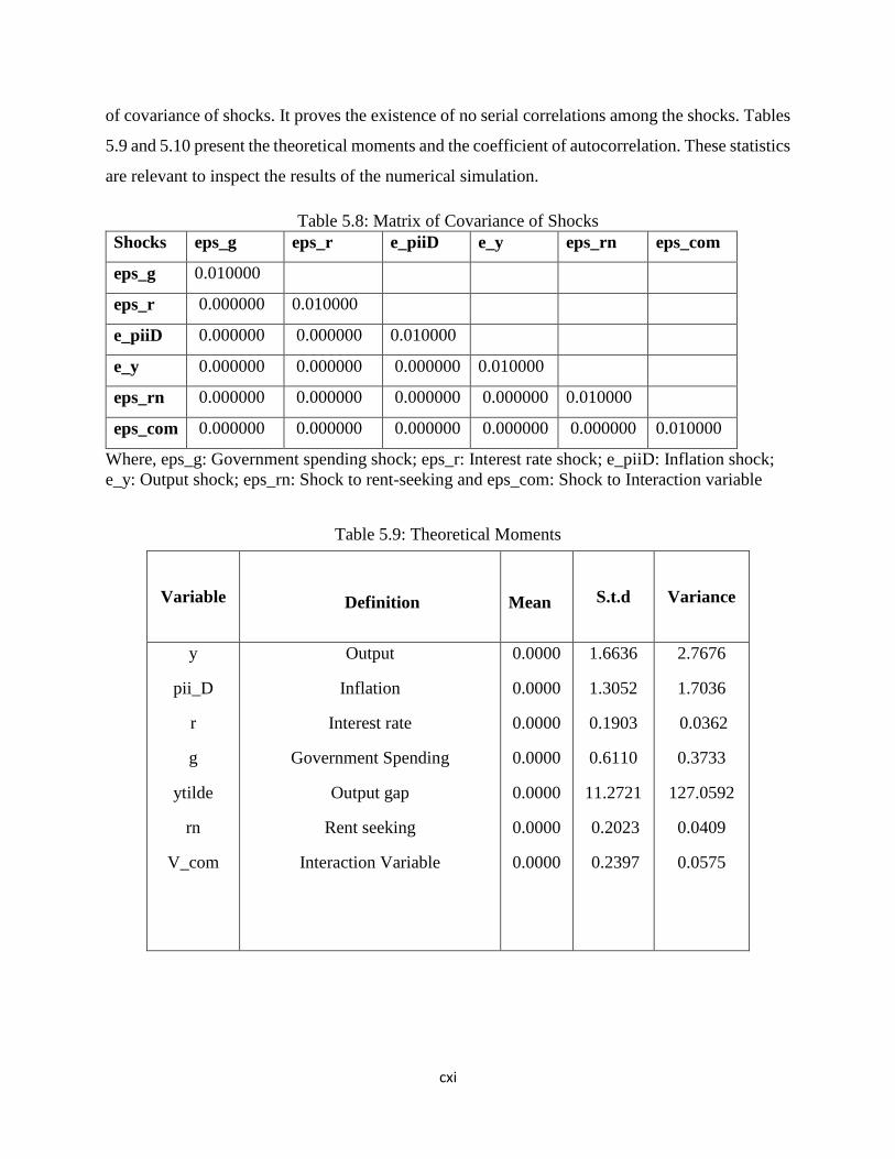
cxi
of covariance of shocks. It proves the existence of no serial correlations among the shocks. Tables
5.9 and 5.10 present the theoretical moments and the coefficient of autocorrelation. These statistics
are relevant to inspect the results of the numerical simulation.
Table 5.8: Matrix of Covariance of Shocks
Shocks eps_g eps_r e_piiD e_y eps_rn eps_com
eps_g 0.010000
eps_r 0.000000 0.010000
e_piiD 0.000000 0.000000 0.010000
e_y 0.000000 0.000000 0.000000 0.010000
eps_rn 0.000000 0.000000 0.000000 0.000000 0.010000
eps_com 0.000000 0.000000 0.000000 0.000000 0.000000 0.010000
Where, eps_g: Government spending shock; eps_r: Interest rate shock; e_piiD: Inflation shock;
e_y: Output shock; eps_rn: Shock to rent-seeking and eps_com: Shock to Interaction variable
Table 5.9: Theoretical Moments
Variable
Definition
Mean
S.t.d
Variance
y
pii_D
r
g
ytilde
rn
V_com
Output
Inflation
Interest rate
Government Spending
Output gap
Rent seeking
Interaction Variable
0.0000
0.0000
0.0000
0.0000
0.0000
0.0000
0.0000
1.6636
1.3052
0.1903
0.6110
11.2721
0.2023
0.2397
2.7676
1.7036
0.0362
0.3733
127.0592
0.0409
0.0575

cxii
Table 5.10: Coefficient of Autocorrelation
Variable Definition 1 2 3 4 5
Y Output 0.6005 0.3790 0.2407 0.1528 0.0964
pii_D Inflation 0.0464 0.0293 0.0202 0.0151 0.0116
R Interest rate 0.8281 0.6439 0.4884 0.3659 0.2721
G Government
spending
0.8132 0.6032 0.4324 0.3057 0.2149
Ytilde Output gap 0.0219 0.0156 0.0098 0.0069 0.0051
Rn Rent seeking 0.8264 0.6164 0.4429 0.3134 0.2204
v_com Interaction
variable
0.7701 0.5464 0.3753 0.2541 0.1708
The nature of interdependence between fiscal and monetary policy is found from the direction and
magnitude of the correlation between both policy variables. The correlation matrix presented in
Table 5.11, obtained from the dynamic simulation of the NK DSGE model, reveals a strong but
negative correlation between fiscal and monetary policy. This shows that both policies are strong
substitutes. The result negates that of Chuku (2010) who conclude that fiscal and monetary policy
act as weak substitutes. The Impulse Response function obtained from the Bayesian estimation as
presented in Figure 5.2 also corroborates the findings of the correlation matrix. It is such that,
although, fiscal and monetary policy acted as substitutes from period 1 to 7 and as complements
from period 8 to 20, the magnitude of the negative interactions between both policies may have
outweighed their complementary interactions. In an overall manner, over the sample period, both
fiscal and monetary policies interacted, therefore, as strong substitutes. This implies that when the
fiscal (monetary) policymaker implements the expansionary measure, the monetary (fiscal)
authority counters this action using contractionary policy.
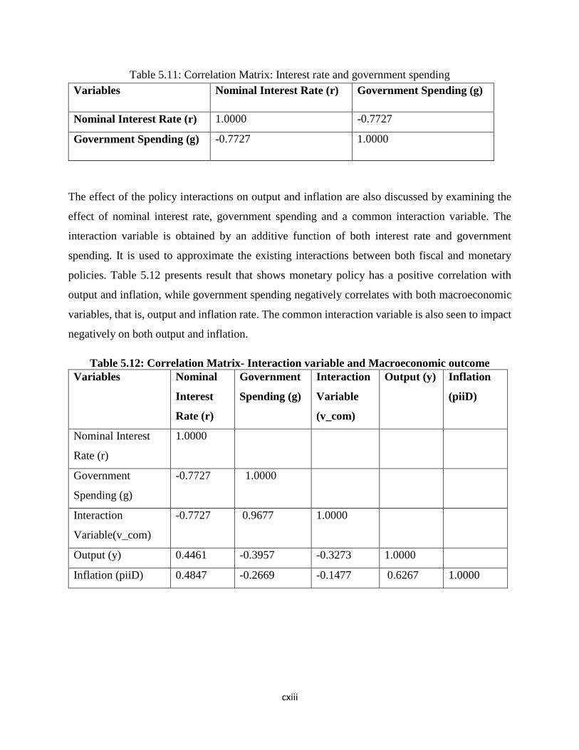
cxiii
Table 5.11: Correlation Matrix: Interest rate and government spending
Variables Nominal Interest Rate (r) Government Spending (g)
Nominal Interest Rate (r) 1.0000 -0.7727
Government Spending (g) -0.7727 1.0000
The effect of the policy interactions on output and inflation are also discussed by examining the
effect of nominal interest rate, government spending and a common interaction variable. The
interaction variable is obtained by an additive function of both interest rate and government
spending. It is used to approximate the existing interactions between both fiscal and monetary
policies. Table 5.12 presents result that shows monetary policy has a positive correlation with
output and inflation, while government spending negatively correlates with both macroeconomic
variables, that is, output and inflation rate. The common interaction variable is also seen to impact
negatively on both output and inflation.
Table 5.12: Correlation Matrix- Interaction variable and Macroeconomic outcome
Variables Nominal
Interest
Rate (r)
Government
Spending (g)
Interaction
Variable
(v_com)
Output (y) Inflation
(piiD)
Nominal Interest
Rate (r)
1.0000
Government
Spending (g)
-0.7727 1.0000
Interaction
Variable(v_com)
-0.7727 0.9677 1.0000
Output (y) 0.4461 -0.3957 -0.3273 1.0000
Inflation (piiD) 0.4847 -0.2669 -0.1477 0.6267 1.0000
cxiv
5.4 Optimal Fiscal and Monetary Policy
In this Section, the optimal Ramsey and discretionary paths of fiscal and monetary policy are
numerically investigated. The optimal fiscal and monetary policy is defined as the path of
government spending and nominal interest rates that minimise the welfare loss of the policymaker
given the constraints posed by the structural equations of the small open economy. The welfare
function of the policymaker is such that both policy makers jointly desire to minimise the
deviations of actual values of inflation, output and government spending from their target values.
The implication of various assumptions on the behaviour of fiscal policy such as rent-seeking,
benevolent, commitment and discretionary, on the optimal paths are specifically examined.
The moments of the optimal policies under different assumptions are presented in Table 5.13. The
moments are computed from dynamic simulations, specifically using the Linear Quadratic method.
The Linear Quadratic approach takes a first-order Taylor approximation to the constraint equations
and a quadratic approximation to the objective function. To this end, Dynare 4.5.1 routines on
Ramsey and Discretionary Policy are used for the numerical simulations

cxv
Table 5.13: Moments of Optimal Fiscal and Monetary Policy
A. Ramsey with Benevolent Fiscal Policy (Benchmark)
Variable Standard
deviation
Autocorrelation Welfare Loss
Government Spending
Nominal Interest Rate
0.138
0.034
0.700
0.139
0.176
B. Ramsey with Rent seeking Fiscal Policy
Variable Standard
deviation
Autocorrelation Welfare Loss
Government Spending
Nominal Interest Rate
0.297
0.034
0.621
0.128
0.806
C. Discretionary with Benevolent Fiscal Policy
Variable Standard
deviation
Autocorrelation Welfare Loss
Government
Spending
Nominal Interest
Rate
0.139
0.035
0.698
0.165
0.179
D. Discretionary with Rent seeking Fiscal Policy
Variable Standard deviation Autocorrelation Welfare Loss
Government
Spending
Nominal Interest
Rate
0.297
0.034
0.621
0.128
0.806
The Ramsey outcomes show the dynamic properties of optimal policy when policymakers commit
to specified rules for current and future dates. In the benchmark model, government spending and
interest rates are 13.8 and 3.4 percentage points volatile. Government spending is also found to be
more persistent than the nominal interest rate. Furthermore, the welfare loss is 0.176. In
comparison with the other models (B, C and D), the Ramsey policy with the benevolent
government has the least volatile paths for both fiscal and monetary policy instruments. It can then
be adjudged to have the most macroeconomic stable property. Table 5.13 also reveals that the
cxvi
optimal policies are more volatile in models with rent-seeking assumptions. This implies that the
rent-seeking tendencies of government can be a source of volatility. It can also be deduced from
the table that the discretionary form of policy has a trivial impact on the sequence of optimal fiscal
and monetary policy.
Furthermore, the value of the loss function of the policymakers at 0.806 is higher in models with
rent-seeking assumptions than in the model with benevolent government at 0.176 and 0.179. This
means model economies with rent-seeking tendencies are more welfare-reducing than those of
economies with a benevolent government. In summary, the benchmark model, that is, Ramsey
Policy with benevolent government has the most desirable path for optimal fiscal and monetary
policy. An economic implication of this result is that the Nigerian government ought to commit to
policy rules and should implement policies that are expected to maximise economic welfare for
all, not just a subset of its citizens.
5.5 Implication of Findings
A New Keynesian DSGE model has been simulated and estimated in this chapter using Dynare
codes. The model is a system of 27 equations with 27 endogenous variables and coincidentally,
27 parameters were calibrated to mimic the Nigerian economy.
The main results obtained from this study include:
(1) The parameter value of the reaction of inflation to the changes in interest rate (υπ) is less than
one, while the reaction of output to the Taylor rule (υy) has a higher magnitude. This indicates the
existence of a passive monetary policy such that the Central Bank has to adjust its policy decisions
to suit fiscal behaviour. The second implication of this result is that the Central Bank has not been
primarily implementing policies for price stability, but for output stability.
(2) The parameter value of the degree of rent-seeking (𝜒) suggests that only a trivial proportion of
government expenditure was actually expended for welfare-enhancing projects, the remainder is
suspected to have been wasted, misused or stolen.
(3) The study also found that both fiscal and monetary policies act as strong substitutes. This means
that when one policymaker implements an expansionary measure, the other counters this action

cxvii
using contractionary policy. This contrasts with Chuku (2010) who used the Markov-switching
model and find that fiscal and monetary policy act as weak substitutes
(4) The common variable that explicitly captures the interaction between fiscal policy and
monetary policy shows that the joint process of both policies has a weak but negative effect on
output and inflation. This result can be interpreted in two ways. The first implication is that actual
policy implementation in Nigeria that captures the rent seeking and discretionary nature of the
federal government coupled with existing weak policy coordination, have sub-optimal impact on
the Nigerian economy. The result also shows on the other hand, that stabilisation policies may be
inadequate in influencing the outcomes of output and inflation in Nigeria.
(5) The optimal fiscal and monetary policy are characterised by a regime where the fiscal policy
maker is benevolent and commits to a policy rule while the Central Bank commits to its monetary
policy rule. Rent seeking activities considerably reduces welfare by over 357 percent when
compared with the welfare loss from a benevolent government. Therefore, rent- seeking activities
have a non-trivial implication for the path of optimal fiscal and monetary policy.

cxviii
CHAPTER SIX
CONCLUSION AND RECOMMENDATION
6.1 Summary
The renewed interest of policymakers in implementing fiscal measures towards economic
stabilisation, in the aftermath of the 2008/2009 global financial crisis, has sparked attention on the
issue of fiscal and monetary policy interactions. In Nigeria, policymakers are also concerned about
the alignment of fiscal and monetary policy coupled with a consistent policy design. Chuku (2010);
Musa et al., (2013) and Adeboye (2015) have investigated the interactions between fiscal and
monetary policy in Nigeria. However, existing evidence on government's fiscal behaviour shows
that conventional assumptions such as benevolent spending, rule-based fiscal process and policy
coordination, should be modified in line with the political economy literature (Fragetta and
Kirsanova, 2010; Dimakou, 2015; Miller, 2016). This study, therefore, argued that the rent-seeking
tendency of fiscal policymakers, the discretionary power of government and weak policy
coordination have implications in accounting for the interaction between fiscal and monetary
policies.
Following this background, the study sought to examine fiscal and monetary policy interaction
under alternative assumptions of a rent-seeking government that follows discretionary policies and
where no economic policy coordination exists. Its specific objectives were to assess the nature of
fiscal policy interactions with monetary policy in Nigeria; examine the transmission effect of the
policy interactions on output and inflation and investigate the optimal fiscal and monetary policy
mix that guarantees economic stability in Nigeria. To this end, the study tested the null hypotheses
that include: (1) Fiscal policy has no interaction with monetary policy in Nigeria; (2) There is no
transmission effect of the policy interaction on output and inflation in Nigeria; (3) There is no

cxix
optimal fiscal and monetary policy mix for output and inflation stability in Nigeria over the
quarterly period of 1961Q1 to 2016Q4.
The study hinged on the New Keynesian School of economic thought. The New Keynesian model
maintains traditional Keynesian postulations such as imperfect competition and sticky prices. In
addition, they propose the use of micro-founded models that assume forward-looking and
optimising economic agents. The study, to this end, adopted the use of a New Keynesian dynamic
general equilibrium model. Features such as habit formation, Non-Ricardian households and a
discretionary rent seeking fiscal behaviour were added to the canonical New Keynesian Dynamic
Stochastic General Equilibrium model, in order to adapt the model to the Nigerian economy.
To achieve the three specific objectives of the study, the Bayesian estimation method was used. In
addition to it, numeric simulations based on log-linear Taylor approximation method and the linear
quadratic technique were adopted. The Bayesian method was used to test the quarterly empirical
data on Nigeria and the United States, over the period 1961Q1 to 2016Q4 on relevant
macroeconomic policy variables. The relevant variables include the Real Gross Domestic Product,
Consumer Price Index, Terms of trade, Nominal interest rate, Government Expenditure. Also, the
Real Gross Domestic Product (RGDP) series for the United States was used as proxy for the
foreign economy.
The Bayesian method was employed to estimate the New Keynesian Dynamic Stochastic General
Equilibrium model. Numerical simulations were also used to empirically characterise the nature
of policy interactions and measure the effect of this interaction on output and inflation. The
dynamic simulation essentially the linear quadratic approach to Ramsey and discretionary optimal
policy was used to obtain the optimal paths of both the fiscal and monetary policy. Answers found
using the estimation and simulation techniques established the significance of the study. Therefore,
the study was able to characterise the interrelation between both fiscal and monetary policies.
Secondly, it was able to identify the transmission effects of fiscal actions on monetary policy and
the aggregate economy. Consequently, this study was novel in testing the implication of alternative
assumptions for fiscal-monetary policy interactions. Secondly, the study was also novel in
constructing an interacting variable in order to explicitly measure the interaction between both
policies.

cxx
6.2 Major Findings of the Study
Chapters 3 and 5 are the primary source of findings in this study. Using the requisite descriptive
statistics, the stylised facts established among other facts, that there is positive correlation between
fiscal and monetary policy. It also found that there are indications for rent-seeking in Nigeria. In
addition, fiscal and monetary policies were seen to have been weakly coordinated in Nigeria and
finally, it found evidence of discretionary fiscal policy in Nigeria. The study also presented
relevant estimation and simulation results. The Bayesian estimation method and numerical
simulations were used to answer the first research question ‘To what extent does fiscal policy
interacts with monetary policy in Nigeria?’ The results show, contrary to findings of the stylised
facts that fiscal policy correlates strongly but negatively with monetary policy in Nigeria.
A numeric simulation using the log-linearisation method was used to answer the second research
question ‘What is the transmission effect of the policy interaction on output and inflation in
Nigeria?’ To answer this question, a common interaction variable was constructed to explicitly
capture fiscal-monetary policy interactions. The study found out that the joint process of both
policies had a weak but negative effect on output and inflation. Finally, a dynamic simulation
applying the Linear Quadratic approximation method was employed to address the third research
question ‘How should fiscal and monetary policy be optimally combined for output and inflation
stability in Nigeria?’ The result showed that the optimal fiscal and monetary policy is characterised
by a regime where the fiscal policy maker is benevolent and commits to a policy rule while the
Central Bank commits to its monetary policy rule. Other major results from the study shows that
the parameter value of the reaction of inflation to the changes in interest rate is less than one, while
the reaction of output to the Taylor rule has a higher magnitude. Furthermore, a low parameter
value for the degree of rent-seeking suggests a high rate of rent-seeking among politicians and
bureaucrats.
6.3 Recommendations
To reiterate the main findings: Firstly, there is a strong and negative correlation between fiscal and
monetary policy; secondly, joint policy interaction has a weak but negative effect on the
macroeconomy. Thirdly, the most desirable nature of fiscal and monetary policy is one where a
cxxi
benevolent government commits to policy rule and where the central bank also commits to its
Taylor rule.
A political economic implication of the strong and negative correlation between fiscal and
monetary policies means that both fiscal policy and monetary policy act as strong substitutes. This
indicates that when one policymaker implements an expansionary measure, the other counters this
action using contractionary policy. It, therefore, implies that policymakers have in the past,
implemented conflicting and uncoordinated fiscal and monetary measures. This can be a potential
source of instability to the economy. This conflicting form of policy implementation occurred in
the divergent response of the Federal Government and the Central Bank to the recent recessionary
episode in 2016. In this instance, the Federal Government adopted an easy fiscal stance by
increasing the amount of budget deficit, while, the Central Bank of Nigeria tightened its monetary
stance by raising the Monetary Policy Rate.
The negative effect of the joint policy interaction on inflation and output implies that the overall
impact of policy interaction negatively affects both long run and short run economic outcomes. Its
weak effect also signals that actual policy implementation in Nigeria that captures the rent-seeking
and discretionary nature of the federal government coupled with existing weak policy
coordination, have sub-optimal impact on the Nigerian economy. Furthermore, the result shows
that asides stabilisation policies, other measures such as structural policies are, therefore, suspected
to significantly account for the outcomes in output and inflation. These structural policies include
but are not limited to trade policy and financial policy. The result on the optimal fiscal-monetary
combination points out that politicians and bureaucrats in government should take caution on
policy reversals by committing to policy rules and at the same time, should implement policies
that enhance the welfare of the entire citizens, not just a subset of the citizens.
Furthermore, the parameter estimates of the coefficients in the Taylor rule indicate the existence
of a passive monetary policy regime. It means that the Central Bank has to adjust its policy
decisions to suit government's fiscal decisions. The second implication of this result is that the
Central Bank has not primarily implemented policies for price stability, but for output stability.
This may also be viewed from the perspective that the Central Bank of Nigeria may not have
adopted policy measures that effectively transmit into affecting domestic prices in the economy.

cxxii
The economic implication of the high degree of rent-seeking among politicians and bureaucrats is
that only a trivial proportion of government expenditure is actually expended for welfare-
enhancing projects, the remainder is wasted, misused or stolen. For instance, the Minister of
Information, Lai Mohammed, argued that a sizeable proportion of stolen public funds by former
politicians and bureaucrats between 2006 and 2013, could have provided 635.18 kilometres of
road; built thirty-six ultra-modern hospitals; erected 183 schools; educated 3,974 children from
primary school to University; and provided 20,062 units of 2-bedroom houses, in order to ease
accommodation.
Based on the implications of the major findings of this study, it is necessary that political economy
scholars and the government consider the following measures:
a. The Central Bank of Nigeria and Federal Ministry of Finance can improve existing
coordination mechanisms using evidence-based planning and forecasting through the
adoption of sophisticated economic models such as the Dynamic Stochastic General
Models.
b. In relation to (a), the Central Bank of Nigeria and Federal Ministry of Finance can
harmonise their policy decisions by mutually adopting the same economic model and/ or
assumptions to guide the planning and forecasting of their target values.
c. The results show that stabilisation policies, that is, fiscal and monetary policy are
inadequate towards guiding the macroeconomy. These policies ought to be complemented
with structural policies such as trade policy and financial policy. A study considering and
comparing the impact of each variant of policy is, therefore, suggested
d. Politicians, bureaucrats and legislators alike, should evaluate policies using evidence-based
models before deciding on policy reversals. Moreover, more effective and non-partisan
anti-corruption programs should be adopted, in order, to discourage rent-seeking.

cxxiii
6.4 Contributions to Knowledge
It is worthy of note that this study contributed to knowledge, by filling the following research gaps:
Firstly, the study explicitly modelled alternative fiscal assumptions within a DSGE model for
Nigeria. This is important to reflect the political economic reality of policymaking and then,
explore how it affects the interaction between fiscal and monetary policy. This meant that the study
adopted a political economy approach to economic policymaking. Secondly, the study constructed
a common variable in order to explicitly measure the joint processes of fiscal and monetary policy
interactions. This is to enable the measurement of the transmitted effect of policy interaction on
both inflation and output.
In another dimension, the study also contributed to knowledge by adding to the relatively
unexplored literature on fiscal-monetary policy interaction in Nigeria, especially within the context
of modelling the fiscal behaviour of government using realistic assumptions and the application of
the Dynamic Stochastic General Equilibrium framework in a Small Open economy environment.
6.5 Suggestions for Further Research
In a political economy environment typified by rent-seeking, a discretionary pattern of policy
actions and weak policy coordination, it is expected that these factors will be relevant in altering
the overall impact of macroeconomic policies. In line with this, some parameter estimates in this
study were somewhat inconsistent with Adegboye (2015), who consider fiscal-monetary policy
interactions under the conventional assumptions. Future studies can, therefore, compare the results
of policy interaction, using both diverging conventional and alternative assumptions. Secondly,
since both fiscal and monetary policies are found to have a weak effect on the economy, future
studies can investigate and compare the magnitude of structuralist policies vis-a-vis stabilisation
policies.
Moreover, subsequent research can examine Markov-switching fiscal and monetary policies. This
captures richer dynamics in the behaviour of these policies since it shows that policy parameters
are not constant over a horizon but can vary over time. Furthermore, the Linear Quadratic method
finds zero mean values for variables, therefore, the actual values of optimal policy variables cannot
be measured. Hence, subsequent studies can consider optimal fiscal and monetary policy using a
non-linear system of equations, in order to overcome this fallout. Finally, other researchers can

cxxiv
also examine the interactions between fiscal and monetary policies using data for the sub-national
government such as states in the Nigerian Federation. This is because the fiscal decisions of state
governments can also be significant for the aggregate economy of Nigeria.
cxxv
REFERENCES
Adams, K. and Billi, R. M. (2008). Monetary conservatism and fiscal policy. The Federal Reserve
Bank Economics Research Department Working Paper 07-01. Available from:
https://pdfs.semanticscholar.org/94cc/54ef8abe1a2d9eaa95b82398d4412ee7c147.pdf.
Adebiyi, M. A. and Mordi, C. N. O. (2010). Estimating small scale macroeconometric model
(SSMM) for Nigeria: A dynamic stochastic general equilibrium (DSGE) approach. Central Bank
of Nigeria Occasional Paper, 39:1-45. Available from:
https://ecomod.net/sites/default/files/document-conference/ecomod2010/1066.doc.
Adebiyi, M.A. and Mordi, C.N.O. (2016). A dynamic stochastic general equilibrium (DSGE)
model of exchange rate pass-through to domestic prices in Nigeria. Occasional Paper 59, Research
Department, Central Bank of Nigeria. Available from:
https://www.cbn.gov.ng/out/2017/rsd/occasional%20paper,%2059%20combined.pdf.
Adegboye, A. A. (2015). Effects of fiscal and monetary policy interactions on inflation and output
in Nigeria (1961-2011) (Doctoral dissertation). Obafemi Awolowo University, Ile-Ife, Nigeria.
Agu, C. (2007). What does the central bank of Nigeria target? An analysis of monetary policy
reaction function in Nigeria. In: Biannual Research Workshop of the African Economic Research
Consortium, Arusha Tanzania, October 2007.
Ajayi, S. I. (1974). An econometric case study of the relative importance of monetary and fiscal
policy in Nigeria. The Bangladesh Economic Review, 2(2):559-576.
Ajisafe, R. A. and Folorunso, B. A. (2002). The relative effectiveness of fiscal and monetary policy
in macroeconomic management in Nigeria. The African Economic and Business Review, 3(1): 23-
40.
Alege, P. O. (2008). Macroeconomic policies and business cycle in Nigeria: 1970-2004 (Doctoral
dissertation). Covenant University, Ota, Nigeria.
Alege, P. O., (2012). A Business Cycle Model for Nigeria. Journal of Applied Statistics, 3(1):85-
115.
Alesina, A. and Tabellini, G. (1987). Rules and discretion with non-coordinated monetary and
fiscal policy. Economic Inquiry, 25: 619-630.
Algozhina, A. (2012). Monetary and fiscal policy interactions in an emerging open economy: A
non-Ricardian DSGE approach. CERGE-EI Working Paper Series 476. Available from:
https://www.cerge-ei.cz/pdf/wp/Wp476.pdf.
Almeida, V. (2010). Bayesian estimation of a DSGE model for the Portuguese Economy. Working
Paper, Economic Research Department, Banco de Portugal. Available from:
http://ssrn.com/abstract=1535285.

cxxvi
An, S. and Schorfheide, F. (2006). Bayesian analysis of DSGE models. Available from:
https://www.philadelphiafed.org/research-and-data/.../2006/wp06-5.pdf.
Anas, M. (2013). Monetary and fiscal policy in an estimated DSGE model for Morocco. British
Journal of Science, 9(1): 1-17.
Anyanwu, J.C. (1999). Fiscal relations among the various tiers of government in Nigeria.
Available from:http://www.researchgate.net/publication/263662301.
Anyanwu, J.C., Oyefusi, A., Oaikhenan, H. and Dimowo, F.A. (1997). The structure of the
Nigerian economy (1960-1997). Joanee Educational Publishers Ltd.
Ascari, G., Florio, A. and Gobbi, A. (2016). Monetary and fiscal policy interactions: Leeper (1991)
redux. University of Oxford Department of Economics Discussion Paper Series 788. Available
from: https://www.economics.ox.ac.uk/materials/papers/14431/paper-788.pdf.
Azzimonti, M., Battaglini, M and S. Coate, (2016). The costs and benefits of balanced budget
rules: Lessons from a Political Economy Model of Fiscal Policy, Journal of Public Economics,
136:45–61.
Bartolomeo, G. and Gioacchino, D. (2004). Fiscal-monetary policy coordination and debt
management: A two stage dynamic analysis. Università DegliStudi Di Roma “La Sapienza”
Dipartimento Di Economia Pubblica Working Paper 74. Available from:
https://www.researchgate.net/publication/23747779_Fiscal-
Monetary_Policy_Coordination_And_Debt_Management_A_Two_Stage_Dynamic_Analysis
Barseghyan, L., Battaglini, M. and Coate, S. (2013). Fiscal policy over the real business cycle: A
positive theory. Journal of Economic Theory, 148(6):2223-2265.
Benigno, P. and Woodford, M. (2004). Optimal monetary and fiscal policy: A linear-quadratic
approach. NBER Macroeconomics Annual 2003, Eds Gertler, M. and Rogoff, K. The MIT Press.
ISBN: 0-262-07253-X. Available from: http://www.nber.org/books/gert04-1.
Bergholt, D. (2012). The Basic New Keynesian Model January. Available from:
https://bergholt.weebly.com/uploads/1/1/8/4/11843961/the_basic_new_keynesian_model_-
_drago_bergholt.pdf.
Bianchi, F. and Ilut, C. (2016). Monetary/fiscal policy mix and agents beliefs. Available from:
www.nber.org/papers/w20194.
Blanchard, O.J. and Kahn, C.M. (1980). The solution of linear difference models under rational
expectations. Econometrica, 48(5):1305-1311. Available from:
http://www.jstor.org/stable/1912186. .

cxxvii
Blinder, A. S. (1982). Issues in the coordination of monetary and fiscal policies. In: Proceedings-
Economic Policy Symposium-, Federal Reserve Bank of Kansas City, pp: 3-46.
Budget Office of the Federation (2016). Budget. Available from:
http://www.budgetoffice.gov.ng/index.php/resources/internal-resources/budget-documents
Buiter, W. (1999). The fallacy of the fiscal theory of the price level. NBER Working Paper 7302.
Available from: www.nber.org/papers/w7302
Buiter, W.H. (2002). The fiscal theory of the price level: A critique. The Economic Journal,
112(481): 459-480.
Calvo, G.A. (1983). Staggered prices in a utility-maximizing framework. Journal of Monetary
Economics, 12: 383-398.
Canzoneri,M.B, Cumby R E. and Diba, B.T. (2001). Is the price level determined by the needs of
fiscal solvency? The American Economic Review, 91(5):1221-1238.
Carlson, K.M. (1982). The mix of monetary and fiscal policies: conventional wisdom vs.
empirical reality. Review, 64(8):7-21.
Cass, D. (1965). Optimum growth in an aggregative model of capital accumulation. Review of
Economic Studies, 32: 233-240.
Cazacu, A., (2015). Fiscal-monetary policy interaction. SVAR Evidence from a CEE country.
European Scientific Journal, :12-23.
Çebi, C. (2011). The interaction between monetary and fiscal policies in turkey: An estimated
new Keynesian DSGE model. Central Bank of the Republic of Turkey Working Paper
11(04). Available from: https://ideas.repec.org/p/tcb/wpaper/1104.html.
Cekin, S.E. (2013). Monetary and fiscal policy interactions in turkey: A Markov switching
approach. In: Thirteenth Annual Missouri Economics Conference. University of Missouri and
the Research Division of the Federal Reserve Bank of St. Louis, 22 - 23 March 2013. Available
from: https://files.stlouisfed.org/files/htdocs/.../2013/Cekin_FRB_conference%20paper.pdf.
Central Bank of Nigeria (1958). Central Bank of Nigeria Act,1958. Available from:
https://en.wikipedia.org/wiki/Central_Bank_of_Nigeria_Act_1958
Central Bank of Nigeria (1991). Central Bank of Nigeria Act, 1991. Available from:
https://www.cbn.gov.ng/OUT/PUBLICATIONS/BSD/1991/CBNACT.PDF
Central Bank of Nigeria (2006). Communiqué No. 48 of the Monetary Policy Committee.
Available from: https://www.cbn.gov.ng/OUT/CIRCULARS/MPD/2007/MPC-48.PDF
Central Bank of Nigeria (2007). Central Bank of Nigeria Act. Available from:
www.cbn.gov.ng/out/publications/bsd/2007/cbnact.pdf
cxxviii
Central Bank of Nigeria (2011a). Understanding monetary policy series no 3. Central Bank of
Nigeria monetary policy framework. Available from:
https://www.cbn.gov.ng/out/2012/ccd/series%203.pdf
Central Bank of Nigeria (2011b). Understanding monetary policy series no 5. Monetary and fiscal
policy coordination. Available from:
https://www.cbn.gov.ng/Out/2014/MPD/UNDERSTANDING%20MONETARY%20POLICY%
20SERIES%20NO%205.pdf
Central Bank of Nigeria Statistical Bulletin (2013). Available from:
http://www.cbn.gov.ng/documents/Statbulletin.asp
Central Bank of Nigeria Statistical Bulletin (2015). Available from:
http://www.cbn.gov.ng/documents/Statbulletin.asp
Central Bank of Nigeria (2015a). FAQ on monetary policy. Available from:
https://www.cbn.gov.ng/FAQS/FAQ.asp?Category=Monetary+Policy
Central Bank of Nigeria (2015b). Conduct of fiscal policy. Available from:
https://www.cbn.gov.ng/MonetaryPolicy/Fiscal.asp
Central Bank of Nigeria Statistical Bulletin (2016). Available from:
http://www.cbn.gov.ng/documents/Statbulletin.asp
Central Bank of Nigeria (2017). Communiqué No. 112 of the Monetary Policy Committee.
Available from:
https://www.cbn.gov.ng/Out/2017/MPD/Central%20Bank%20of%20Nigeria%20Communique%
20No%20112%20Monetary%20Policy%20Committee%20Meeting%20March%2021%202017.p
df
Cevik, E. I., Dibooglu, S. and Kutan, A.M. (2014). Monetary and fiscal policy interactions:
Evidence from emerging European economies. Journal of Comparative Economics, 42(4):1079-
1091.
Chadla, J. S., and Nolan, C. (2003). On the interaction of monetary and fiscal policy. Forthcoming
in Dynamic Macroeconomic Theory. - Theory and policy in general equilibrium. (Eds) Sumru
Altug, Jagit S. Chadla and Charles Nolan, Cambridge University Press.
Christiano, L. J. and Terry, J.F. (2000). Understanding the fiscal theory of the price level. NBER
working paper 7688. Available from:www.nber.org/papers/w7668.pdf.
Chen, Z. (2017). Interactions between fiscal and Monetary Policy: A New Keynesian Model with
Regime Switching Process. (Undergraduate Thesis). Available from:
http://publish.wm.edu/honorstheses/1013.

cxxix
Christiano, L.J., Eichenbaum, M. and Evans, C. (2005). Nominal rigidities and the dynamic effects
of a shock to monetary policy. Journal of Political Economy, 113(1):1-45.
Chuku, C. A. (2010). Monetary and fiscal policy interactions in Nigeria: An application of a state
space model with Markov-switching. CBN Journal of Applied Statistics, 1(1):39-51.
Cochrane, J.H. (2001). Long term debt and optimal policy in the price level. Econometrica,
6(1):69-116.
Darby, M.R. (1984). Some pleasant monetarist arithmetic. Federal Reserve Bank of Minneapolis
Quarterly Review, 8(2):15-20.
Davig, T. and. Leeper, M. E (2009). Monetary-fiscal policy interactions and fiscal stimulus. NBER
Working Paper No. 15133. Available from: www.nber.org/papers/w15133.
Davig, T., Leeper, E. M. and Walker, T. B. (2010). Unfunded liabilities and uncertain fiscal
financing. Journal of Monetary Economics, 57:600–619.
Dimakou, O. (2015). Bureaucratic corruption and the dynamic interaction between monetary and
fiscal policy. European Journal of Political Economy, 40(A):57-78.
Dixit, A. and Lambertini, L. (2003). Interactions of commitment and discretion in monetary and
fiscal policies. The American Economic Review, 93(5):1522-1542. Available from
http://www.jstor.org/stable/3132140.
Ehelepola, K. (2014). Optimal monetary and fiscal policy analysis for Sri Lanka; a DSGE
approach. In: International Research Conference 2014. Central Bank of Sri Lanka. Available from:
https://www.cbsl.gov.lk/sites/default/files/Optimal_Monetary_and_Fiscal_Policy_Analysis_for_
Sri%20Lanka_full.pdf.
Englama, A., Tarawalie, A. and Ahortor, C.R.K. (2013). Fiscal and monetary policy coordination
in the WAMZ: Implications for member states’ performance on the convergence criteria. In:
Fourth Annual Conference for Regional Integration in Africa Abidjan, Côte d’Ivoire. Available
from:
https://www.researchgate.net/publication/300366086_Fiscal_and_Monetary_Policy_Coordinatio
n_in_the_WAMZ_Implications_for_Member_States%27_Performance_on_the_Convergence_C
riteria
Federal Government of Nigeria (1999). Nigerian Constitution. Available from:
http://www.nigeria-law.org/ConstitutionOfTheFederalRepublicOfNigeria.htm
Fernández-Villaverde, J. (2009). The econometrics of DSGE models. SERIEs, 1:3–49.
Fernandez-Villaverde, J., Rubio-Ramirez, J. F. and Schorfheide, F. (2016). Solution and
Estimation Methods for DSGE Models. Forthcoming in Handbook of Macroeconomics, 2.
Available from: http://www.nber.org/papers/w21862
cxxx
Fiscal Responsibility Act (2007). Fiscal Responsibility Act. Available
from:http://internationalbudget.org/wp-content/uploads/Nigeria-FiscalResponsibilityAct2007-
English.pdf
Flotho, S. (2009). DSGE models - solution strategies. Available from: https://www.macro.uni-
freiburg.de/publications/research_flotho/dsge_models.
Fragetta, M. and Kirsanova, T. (2010). Strategic monetary and fiscal policy interactions: An
empirical investigation. European Economic Review, 54(7):855-879.
Franta, M., Libich, J. and Stehlik, P. (2012). Tracking monetary-fiscal interactions across time and
space. Czech National Bank Working Paper Series. Available from:
https://www.cnb.cz/en/research/research_publications/cnb_wp/2012/cnbwp_2012_06.html
Gali, J. (2003). New perspectives on monetary policy, inflation, and the business cycle.
Advances in Economics and Econometrics, 3:151-197.
Gali, J. (2008). Monetary policy, inflation, and the business cycle: An introduction to the New
Keynesian framework and its applications. Princeton University Press. ISBN: 9780691164786
Gali, J., and Gertler, M. (1999). Inflation dynamics: A structural econometric analysis. Journal of
Monetary Economics, 44 (2): 195-222. Doi:10.1016/S0304-3932(99)00023-9.
Gali, J. and Monacelli, T. (2005). Monetary policy and exchange rate volatility in a small open
economy. Review of Economic Studies, 72:707–734.
Gali, J., Lopez-Salido, J.D., and Valles, J. (2007). Understanding the effects of government
spending on consumption. Journal of the European Economic Association, 5: 227–270.
Garba, A.G. (2004). Harmonizing fiscal and monetary policy in Nigeria: A preliminary analysis
and suggestion for further research. In: Garba, A.G., Egwaikhide, F., and Adenikinju, A: Leading
Issues of Macroeconomic Management and Development.
Garcia, C.J. (2010). Is the Phillips curve useful for monetary policy in Nigeria? Central Bank of
Nigeria Occasional Paper, 38:1-36.
Gerba, E. and Hauzenberger, K. (2014). Estimating US fiscal and monetary interactions from
Volcker chairmanship to the Great Recession. Available from:
https://www.researchgate.net/publication/272242060_Estimating_US_Fiscal_and_Monetary_Int
eractions_From_Volcker_Chairmanship_to_the_Great_Recession
Gilksberg, B. (2016). Equilibria under monetary and fiscal policy interactions in a portfolio choice
model. Journal of Economic Dynamics and Control,69(C):209-228.

cxxxi
Gnocchi, S. and Lambertini, L. (2016). Monetary commitment and the level of public debt. Bank
of Canada Staff Working Paper 3. Available from:
https://www.banqueducanada.ca/wpcontent/uploads/2016/02/swp2016-3.pdf.
Gonzalez-Astudillo, M. (2013). Monetary-fiscal policy interactions: Interdependent policy rule
coefficients. Finance and Economics Discussion Series Divisions of Research & Statistics and
Monetary Affairs. Federal Reserve Board, Washington, D.C. Available from:
https://ideas.repec.org/p/fip/fedgfe/2013-58.html.
Griffoli, T.M. (2013). An introduction to the solution & estimation of DSGE models. Dynare
version 4 - User Guide. Available from: www.dynare.org/documentation-and-
support/user.../Dynare-UserGuide-WebBeta. pdf.
Guerron-Quintana, P., Inoue, A. and Lutz, K. (2016). Impulse response matching estimators for
DSGE models. HIAS discussion paper. Available from: https://hermes-ir.lib.hit-
u.ac.jp/rs/bitstream/10086/.../070_hiasDP-E-27.pdf.
Hallett, A.H., Libich, J. and Stehlik, P. (2011). Monetary and fiscal policy interaction with various
degrees of commitment. Czech Journal of Economics and Finance, 64(1):1-29.
Hallet, A. H. and Weymark, D. N. (2007). Fiscal leadership and central bank design. The Canadian
Journal of Economics, 40(2):607-627.
Henderson, D.R. (2008). Rent seeking. In: The Concise Encyclopedia of Economics, Henderson,
D.R (Eds.). Indianapolis: Liberty Fund. Available from: http://www.econlib.org/library/.
Enc/RentSeeking.html.
Hetzel, R.L. (2013). The Monetarist-Keynesian debate and the Philips curve: Lessons from the
Great Inflation. Economic Quarterly, 99(2): 83-116.
Hoover, K.D. (2008). New Classical Macroeconomics. In the Concise Encyclopedia of
Economics. 2008. Library of Economics and Liberty. Available from
http://www.econlib.org/library/Enc/NewClassicalMacroeconomics.html
IMF Fiscal Affairs Department. (2017). Fiscal Rules Dataset 1985 - 2015. Available from:
http://www.imf.org/external/datamapper/fiscalrules/map/map.htm.
Iwata, Y. (2009). Fiscal Policy in an estimated DSGE Model of the Japanese economy: Do non-
Ricardian households explain all?. ESRI Discussion paper series. Available from:
http://www.esri.go.jp/jp/archive/e_dis/e_dis216/e_dis216.pdf.
Jahan, S. and Papageorgiou, C. (2014). What is Monetarism? Finance & Development, 51(1).
Available from: http://www.imf.org/external/pubs/ft/fandd/2014/03/basics.htm

cxxxii
Jahan, S., Mahmud, A.S. and Papageorgiou, C. (2014). What is Keynesian economics? Finance &
Development, 51(3). Available from:
http://www.imf.org/external/pubs/ft/fandd/2014/09/basics.htm
Janků, J. and Kappel, S. (2014). The interaction of monetary and fiscal policy in the Countries of
theVisegradgroup.ActaUniversitatisAgriculturaeEtSilviculturaeMendelianaeBrunensis,
62(2):373-381. Available from: http://dx.doi.org/10.11118/actaun201462020373.
Jawadi, F., Mallick, S. K. and Sousa, R. M. (2016). Fiscal and monetary policies in the BRICS:
A panel VAR approach. Economic Modelling, 58:535-542.
King, R. G. and Watson, M. (1997). System reduction and solution algorithms for singular linear
difference systems under rational expectations. Available from:
https://www.Princeton.Edu/~Mwatson/.../Algor6.Pdf.
Kliem, M., Kriwoluzky, A. and Sarferaz, S. (2015). Monetary-fiscal policy interaction and fiscal
inflation: A tale of three countries. KOF Swiss Economic Institute. Available from:
https://ideas.repec.org/p/zbw/iwhdps/iwh-17-15.html.
Kliem, M., Kriwoluzky, A. and Sarferaz, S. (2016). Monetary–fiscal policy interaction and fiscal
inflation: A tale of three countries. European Economic Review, 88(C):158-184.
Kocherlakota, N. and Phelan, C. (1999). Explaining the fiscal theory of the price level. Federal
Reserve Bank of Minneapolis Quarterly Review, 23:14-23.
Koopmans, T. (1965). On the concept of optimal economic growth. The economic approach to
development planning, North-Holland: Amsterdam.
Kydland, F., and Prescott, E. (1982). Time to build and aggregate fluctuations. Econometrica, 50:
1345-1371.
Leeper, E. M. and Zhou, X. (2013). Inflation's role in optimal monetary-fiscal policy. NBER
Working Paper No. 19686. Available from: www.nber.org/papers/w19686.
Leeper, E.M. and Leith, C. (2015). Inflation through the Lens of the Fiscal Theory. Prepared for
the Handbook of Macroeconomics. Eds. Taylor, J.B and Uhlig, H. Elsevier Press.
Leeper, E.M. (1991). Equilibria under ‘active’ and ‘passive’ monetary and fiscal policies. Journal
of Monetary Economics, 27: 129-147.
Leeper, E.M. (2013). Fiscal limits and monetary policy. NBER Working Paper Series18877.
Available from: www.nber.org/papers/w18877.
Li, S.M. and Spencer, A. (2014). Effectiveness of the Australian fiscal stimulus package: A DSGE
analysis. Research Paper No. 1184, Department of Economics, University of Melbourne. ISBN
No 978 0 7340 5020 5.

cxxxiii
Lima, E.R., Maka, A. and Pumar, A. (2012). The effects of fiscal policy and its interactions with
monetary policy in Brazil. Economia 13(1): 149-180.
Long, J. B. and Plosser, C. (1983). Real business cycles. Journal of Political Economy, 91:39-69.
Mankiw, N.G. (2016). Macroeconomics. 9th Edn. Worth Publishers.
Mankiw N. G. and Romer, D. (1991) New Keynesian economics, Vols. I and II. Cambridge MIT
Press.
Masson, P. (2006). Anchors for monetary policy. Available from:
https://www.bis.org/events/cbcd06g.pdf.
McCallum, B.T. (1984). Are bond-financed deficits inflationary? A Ricardian analysis. Journal of
Political Economy, 92(1): 123-135.
Mickelsson, G. (2015). Estimation of DSGE models: Maximum Likelihood vs. Bayesian methods.
Department of Economics, Uppsala University. Available from:
https://ideas.repec.org/p/hhs/uunewp/2015_006.html.
Miller, D. S. (2016). Commitment versus discretion in a political economy model of fiscal and
monetary policy interaction. Journal of Monetary Economics, 84(C):17-29.
Miller, P.J., and Sargent, T.J. (1984). A reply to Darby. Federal Reserve Bank of Minneapolis
Quarterly Review, 8(2): 21-26.
Mirman, L.J and Brock, W.A. (1972). Optimal economic growth and uncertainty: The discounted
case. Journal of Economic Theory, 4: 479-533.
Mishkin, F.S. (2000). From monetary targeting to inflation targeting: Lessons from the
industrialized countries. In: Stabilization and Monetary Policy: The International Experience.
Bank of Mexico, 14-15 November 2000. Available from:
https://www0.gsb.columbia.edu/faculty/fmishkin/PDFpapers/00BOMEX.pdf.
Montoro, C., Takats, C. and James, Y. (2012). Is monetary policy constrained by fiscal policy? In:
Fiscal policy, public debt and monetary policy in emerging market economies, Bank for
International Settlements (Eds.). Bank for International Settlements., pp:11-30.
Mordi, C.N.O., Adebiyi, M.A., Adenuga, A.O., Abeng, M.O., Adeboye, A.A., Adamgbe, E.T. and
Evbuomwan, O.O. (2013). Dynamic stochastic general equilibrium (DSGE) model for
monetary policy analysis in Nigeria. Research Department, Central Bank of Nigeria. Available
from:
https://www.cbn.gov.ng/out/2015/rsd/dynamic%20stochastic%20general%20equilibrium%20mo
del%20for%20monetary%20policy%20analysis%20in%20nigeria.pdf.

cxxxiv
Mundell, R. A. (1962). The appropriate use of monetary and fiscal policy for internal and external
stability. Staff Papers (International Monetary Fund), 9(1): 70-79.
Musa, Y., Asare, B.K. and Gulumbe, S.U. (2013). Effect of monetary-fiscal policies interaction
on price and output growth in Nigeria.CBN Journal of Applied Statistics, 4(1): 55.
Muscatelli, V.A., Tirelli, P. and Trecroci, C. (2002). Monetary and fiscal policy interactions over
the cycle: Some empirical evidence. Available from: https://www.cesifo-
group.de/DocDL/cesifo_wp817.pdf.
Muscatelli, V. A., Tirelli, P. and Trecroci, C. (2005). Fiscal and monetary policy interactions in a
new Keynesian model with liquidity constraints. Available from:
https://www.gla.ac.uk/media/media_22210_en.pdf.
National Bureau of Statistics (2012). Consumption pattern in Nigeria 2009/10, Preliminary Report.
National Bureau of Statistics (2016). Nigerian Gross Domestic Product Report Q3 2016.
Niemann, S. and Hagen, J.V. (2008). Coordination of monetary and fiscal policies: A fresh look
at the issue. Swedish Economic Policy Review, 15: 89-124.
Niemann, S. and Pichler, P. (2010). Optimal fiscal and monetary policy under rare disasters: The
role of government debt and monetary conservatism. Available from:
https://www.researchgate.net/publication/229053244.
Niepelt, D. (2004). The fiscal myth of the price level. The Quarterly Journal of Economics,
119(1): 277-300.
Nordhaus, W.D. (1994). Policy games: Coordination and independence in monetary and fiscal
policies. Brookings Papers on Economic Activity (2). Available from:
https://www.brookings.edu/bpea-articles/policy-games-coordination-and-independence-in
monetary-and-fiscal-policies/
Nunes, A. F. and Portugal, M. S. (2010). Active and passive fiscal and monetary policies: An
analysis for Brazil after the inflation targeting regime. Available from:
www.ufrgs.br/ppge/pcientifica/2010_01.pdf.
Nyamongo, M.E., Sichei, M.M and Mutai, N.K. (2008). The monetary and fiscal policy
interactions in Kenya. Research Department, Central Bank of Kenya.
Oboh, V.U. (2017). Monetary and fiscal policy coordination in Nigeria: A set theoretic approach.
Academic Journal of Economic Studies, 3(1): 48–58.
cxxxv
Okafor, H.C. (2013). Modeling Fiscal-monetary policy interaction in Nigeria. International
Journal of Economics and Finance, 5(1): 86-91.
Olayiwola, K.W. and Osabuohien, E.S. (2011). Fiscal Hydrocephalus and Challenges of Socio-
economic Development in Nigeria. Covenant Journal of Business and Social Sciences, 4(1&2):26-
42.
Olayeni, O.R. (2009). A Small Open Economy Model for Nigeria: A BVAR-DSGE Approach.
Available from: http://mpra.ub.uni-muechen.de/16180
Olekah, J.K. and Oyaromade, R. (2007). Estimating A DSGE model of the Nigerian economy.
Draft paper scheduled for presentation at the 12th African Econometric Society (AES) Conference
in Cape Town, South Africa, July 4-6, 2007. Available from:
http://citeseerx.ist.psu.edu/viewdoc/download?doi=10.1.1.528.9169&rep=rep1&type=pdf.
Onodugo, I. and Amujiri, A. (2015). Towards achieving fiscal responsibility for sustainable
development in Nigeria: A contextual insight. International Journal of Innovative Science,
Engineering & Technology, 2(5): 476-484.
Ornellas, R. and Portugal, M. (2011). Fiscal and monetary interaction in Brazil. Available from:
www.bcu.gub.uy/Comunicaciones/.../t_portugal_marcelo_2011_.pdf.
Persson, T. (2001). Do political institutions shape economic policy? National Bureau of Economic
Research Working Paper 8214. Available from: www.nber.org/papers/w8214.
Petit, M. L. (1989). Fiscal and monetary policy co-ordination: A differential game approach.
Journal of Applied Econometrics, 4(2): 161-179.
Petrevski, G. (2013). The interactions between monetary and fiscal policy: A survey. Available
from: https://www.researchgate.net/publication/258507275.
Pierse, R.G. (2006). Building and solving macroeconomic models using winsolve: Solving DSGE
models. Available from:
www.hkimr.org/uploads/conference_detail/697/con_paper_0_284_hktut3.pdf.
Ramsey, F.P. (1928). A mathematical theory of saving. The Economic Journal, 38 (152):543-559.
Available from: http://www.jstor.org/stable/2224098.
Rasaki, M.G. (2017). A Bayesian estimation of DSGE model for the Nigerian economy.
EuroEconomica, 36(2):145-158.
Reade, J.J. (2011). Modelling monetary and fiscal policy in the US: A cointegration approach.
Department of Economics, University of Birmingham Discussion Paper 11-02. Available
from:https://www.birmingham.ac.uk/Documents/college-social-sciences/.../11-02.pdf.

cxxxvi
Rebelo, S. (2005). Real business cycle models: Past, present, and future. National Bureau of
Economic Research Working Paper 11401. Available from: http://www.nber.org/papers/w11401.
Reserve Bank of India (2013). Fiscal-monetary co-ordination in India: An aassessment. Available
from: https://rbidocs.rbi.org.in/rdocs/Publications/PDFs/5FISCAL250213.pdf.
Romer, D. (2006). Advanced macroeconomics. 3rd Edn., New York: McGraw-Hill.ISBN No
0070536678, 9780070536678.
Rossi, R. (2014). Designing monetary and fiscal policy rules in a new Keynesian model with
rule-of-thumb consumers. Macroeconomic Dynamics, 2(18): 395-417.
Rothenberg, A.D., (2004). The monetary-fiscal policy mix empirical analysis and Theoretical
implications. Available from:
http://citeseerx.ist.psu.edu/viewdoc/download?doi=10.1.1.695.1582&rep=rep1&type =pdf.
Ruge-Murcia, F.J. (2005). Methods to estimate dynamic stochastic general equilibrium models.
Available from:
https://pdfs.semanticscholar.org/e032/efaf5b37de4820487b1c23e5efb7c68ce8ba.pdf.
Sanusi, S.L. (2010). Growth prospects for the Nigerian economy. In: Convocation Lecture,
Igbinedion University, 26 November 2010.
Sargent, T. and Wallace, N. (1981). Some unpleasant monetarist arithmetic. Federal Reserve Bank
of Minneapolis Quarterly Review, 5(3): 1-17.
Saulo, H., Rêgo, L. C. and Divino, J.A. (2013). Fiscal and monetary policy interactions: A game
theoretical approach. Annals of Operations Research, 206(1): 341-366.
Schmitt-Grohe S. and Uribe, M. (2004). Optimal fiscal and monetary policy under sticky prices.
Journal of Economic Theory, 114: 198–230.
Schmitt-Grohe, S., and Uribe, M. (2007). Optimal simple and implementable monetary and fiscal
rules. Journal of Monetary Economics, 54: 1702–1725.
Senbeta, S.R. (2011). A Small Open Economy New Keynesian DSGE model for a foreign
exchange constrained economy. Available from:
https://ideas.repec.org/p/ant/wpaper/2011004.html.
Shahid, M., Qayyum, A. and Shahid, W. (2016). Fiscal and monetary policy interactions in
Pakistan using a dynamic stochastic general equilibrium. Available from: https://mpra.ub.uni-
muenchen.de/72595/.
Serbanoiu, G.V. (2012). Transmission of fiscal policy shocks into Romania's economy. MPRA
paper 40947. Available from: https://mpra.ub.uni-muenchen.de/40947/.
cxxxvii
Sims, C.A. (1994). A simple model for study of the determination of the price level and the
interaction of monetary and fiscal policy. Economic Theory, 4(3):381-399.
Sims, C.A. (1999). The precarious fiscal foundations of EMU. Available from:
sims.princeton.edu/yftp/Amsterdam/EMU.pdf.
Smets, F. and Wouters, R. (2003). An estimated dynamic stochastic general equilibrium model of
the Euro area. Journal of the European Economic Association, 1(5): 1123–1175.
DOI:10.1162/154247603770383415.
Smets, F. and Wouters, R. (2007). Shocks and frictions in US business cycles: A Bayesian
DSGE approach. American Economic Review, 97(3):586-606.
Solow, R. (1956). A contribution to the theory of economic growth. Quarterly Journal of
Economics, 70: 65-94.
Theil, H. (1957). A note on certainty equivalence in dynamic planning. Econometrica, 25(2): 346-
349.
Tinbergen, J. (1952). On the theory of economic policy. North-Holland Publishing Company,
Amsterdam. Available from http://hdl.handle.net/1765/15884.
Torres, J.L. (2015). Introduction to dynamic macroeconomic general equilibrium models.
2nd Edn., Vernon Press. ISBN: 978-1-62273-024-7.
Tovar, C.E. (2008). DSGE models and central banks. Bank for International Settlements Working
Paper 258. Available from: https://www.bis.org/publ/work258.pdf.
Transparency International. (2016). Corruption perception index. Available from:
www.transparency.org/cpi.
Traum, N. and Yang, S. (2011). Monetary and fiscal policy interactions in the post-war U.S.
European Economic Review, 55(1):140-164.
Valdivia, D. and Pérez, D. (2013). Dynamic economic and coordination of fiscal – monetary
policies in Latin America: Evaluation through a DSGE model. Available from:
https://ideas.repec.org/p/pra/mprapa/51562.html.
Vangu, J.K.T. (2014). Do a small open economy DSGE model characterizes correctly the
cyclicality in the African least developed countries? International Household Survey Network
Working Paper.
Walsh, C.E. (2010). Monetary Theory and Policy. 3rd Edn., MIT Press. ISBN No 978-0-262-
01377-2.
cxxxviii
Weil, P. (1987). Permanent budget deficits and inflation. Journal of Monetary Economics, 20: 393-
410.
Woodford, M. (1995). Price level determinacy without control of a monetary aggregate. NBER
Working Paper 5204.
Woodford, M. (1996). Control of the public debt: A requirement for price stability? NBER
Working Paper 5684.
Woodford, M. (2001). Fiscal requirements for price stability. Journal of Money, Credit and
Banking, 33(3): 669-728. Available from: www.gla.ac.uk/media/media_22210_en.pdf.
World Bank (2014). Macroeconomic policy. Available from:
http://www.worldbank.org/en/topic/macroeconomics/brief/macroeconomic policy.
World Development Indicators (2016). Available from: https://datacatalog.worldbank.org/dataset/world-development-indicators
World Governance Indicators (2015). Available from:http://www.govindicators.org.
Wren-Lewis, S. (2011). Comparing the delegation of monetary and fiscal policy. Available from:
https://www.economics.ox.ac.uk/materials/working_papers/paper540.pdf
Yemba, B. (2014). Tax and monetary policy rules in a small open economy with disaggregated
government purchases. Available from: www2.ku.edu/~econ/people/documents/yemba_000.pdf
Yelwa, A.J. (2010). Debt management in Nigeria: Fiscal responsibility and public debt. In: The
process and procedure for obtaining foreign loans by Federal and State Government. House of
Representative Ad-hoc committee on investigation into foreign loans obtained by both the Federal
and State Government, 8 June 2010. Available from:
http://www.nigerianmuse.com/20130907011016zg/nigeria-watch/debt-manageme nt-in-nigeria-
fiscal-responsibility-and-public-debt-by-alhaji-dr-aliyu-jibril-yelwa/

cxxxix
APPENDICES

cxl
Appendix One: Prior
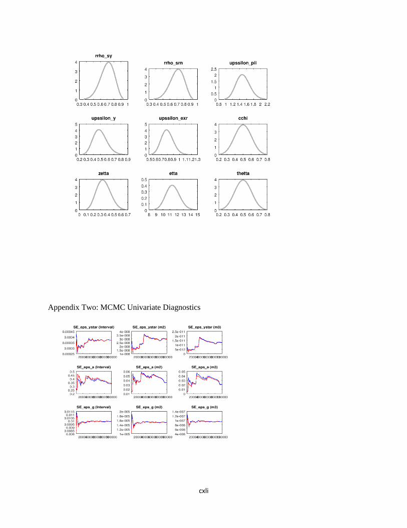
cxli
Appendix Two: MCMC Univariate Diagnostics

cxlii
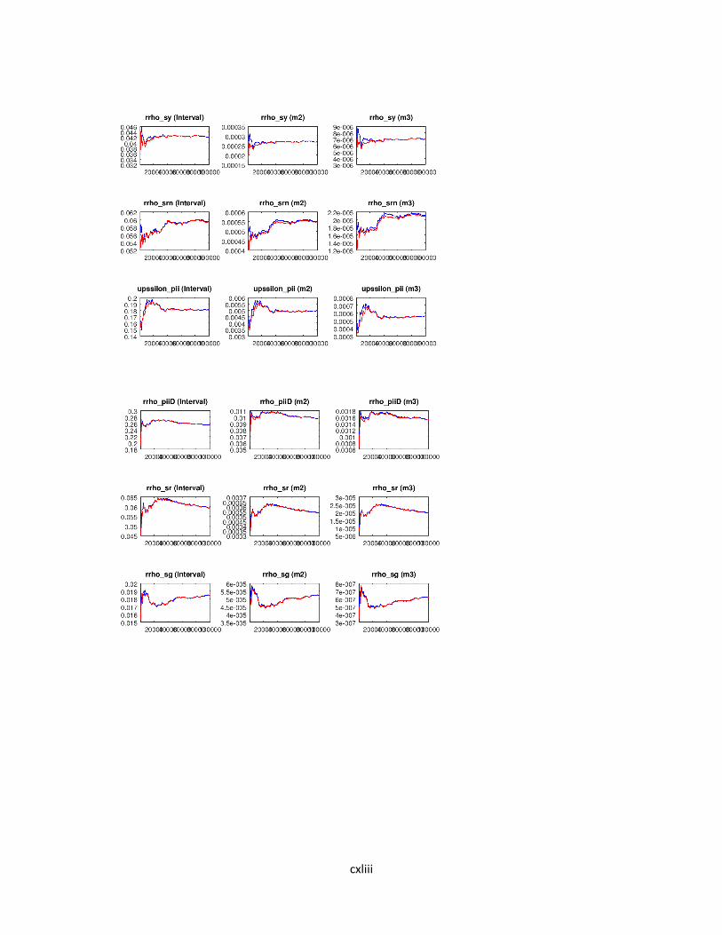
cxliii

cxliv

cxlv
Appendix Three: Dynare Code for Bayesian Estimation
var CR CNR C y pii_D mc s r exr g ytilde pii_F ystar piistar rstar a taxx w NNR TP rn
pii s_piiD s_r s_y s_g s_rn;
varexo eps_g eps_r eps_ystar eps_piistar eps_rstar eps_a eps_taxx eps_TP e_piiD e_y
eps_rn;
parameters h sigmma pssi alphha omegga betta phii rrho_r rrho_ystar rrho_piistar
rrho_rstar rrho_a rrho_taxx rrho_TP cchi zetta gamarr etta thetta upssilon_pii
upssilon_y upssilon_exr kapa_alphha sigmma_alphha paw patp rrho_rn rrho_piiD rrho_sr
rrho_sg rrho_sy rrho_srn;
h=0.7;
sigmma=3.0;
pssi=0.7;
alphha=0.4;
betta=0.95;
phii=4.38;
rrho_r=0.8;
rrho_ystar=0.7;
rrho_piistar=0.7;
rrho_rstar=0.7;
rrho_a=0.7;
rrho_rn=0.3;
rrho_taxx=0.7;
rrho_TP=0.7;
rrho_piiD=0.7;
rrho_sr=0.7;
rrho_sg=0.7;
rrho_sy=0.7;
rrho_srn=0.7;
upssilon_pii=1.5;
upssilon_y=0.5;
upssilon_exr=0.8;
cchi=0.5;
zetta=0.35;
gamarr=0.75;
etta=11.42;
thetta=0.5;
paw=3.2;
patp=1.35;
omegga=((sigmma*gamarr)+(1-alphha)*((sigmma*etta)-1));
sigmma_alphha=sigmma/((1-alphha)+(alphha*omegga));
kapa_alphha=(1-thetta)*(1-(betta*thetta))/(thetta*(sigmma_alphha+phii));
model(linear);
CR-h*CR(-1)=CR(+1)-h*CR-(1-h/sigmma)*(r-pii_D(+1));
CNR=paw*(w+NNR)+(patp*TP);
w=(sigmma/(1-h))*CNR-h*CNR(-1)+phii*NNR;
mc=w-a;
TP=rrho_TP*TP(-1)+eps_TP;
C=pssi*CR+(1-pssi)*CNR;
y=CR+(((alphha*omegga)/sigmma)*s)+g+s_y;
CR-h*CR(-1)=ystar+h*ystar(-1)+(((1-h)*(1-alphha))/sigmma)*s+g;
pii_D=betta*pii_D(+1)+(kapa_alphha*ytilde)+s_piiD;
mc=(sigmma/(1-h))*CR-h*CR(-1)+phii*y-(phii+1)*a+(alphha*s);
s=s(-1)+pii_F-pii_D;
r-rstar=exr(+1)-exr;
exr-exr(-1)=piistar-pii_F;
r=rrho_r*r(-1)+(1-rrho_r)*(upssilon_pii*pii_D+upssilon_y*y+upssilon_exr*(exr-exr(-
1)))+s_r;
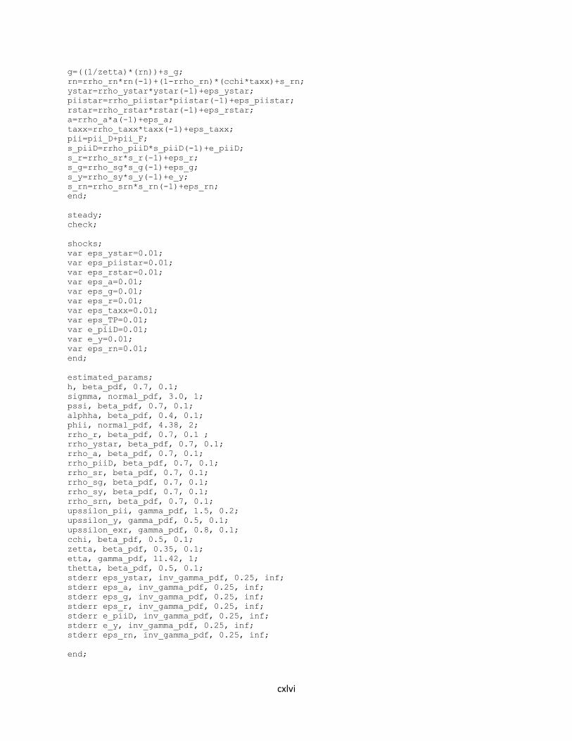
cxlvi
g=((1/zetta)*(rn))+s_g;
rn=rrho_rn*rn(-1)+(1-rrho_rn)*(cchi*taxx)+s_rn;
ystar=rrho_ystar*ystar(-1)+eps_ystar;
piistar=rrho_piistar*piistar(-1)+eps_piistar;
rstar=rrho_rstar*rstar(-1)+eps_rstar;
a=rrho_a*a(-1)+eps_a;
taxx=rrho_taxx*taxx(-1)+eps_taxx;
pii=pii_D+pii_F;
s_piiD=rrho_piiD*s_piiD(-1)+e_piiD;
s_r=rrho_sr*s_r(-1)+eps_r;
s_g=rrho_sg*s_g(-1)+eps_g;
s_y=rrho_sy*s_y(-1)+e_y;
s_rn=rrho_srn*s_rn(-1)+eps_rn;
end;
steady;
check;
shocks;
var eps_ystar=0.01;
var eps_piistar=0.01;
var eps_rstar=0.01;
var eps_a=0.01;
var eps_g=0.01;
var eps_r=0.01;
var eps_taxx=0.01;
var eps_TP=0.01;
var e_piiD=0.01;
var e_y=0.01;
var eps_rn=0.01;
end;
estimated_params;
h, beta_pdf, 0.7, 0.1;
sigmma, normal_pdf, 3.0, 1;
pssi, beta_pdf, 0.7, 0.1;
alphha, beta_pdf, 0.4, 0.1;
phii, normal_pdf, 4.38, 2;
rrho_r, beta_pdf, 0.7, 0.1 ;
rrho_ystar, beta_pdf, 0.7, 0.1;
rrho_a, beta_pdf, 0.7, 0.1;
rrho_piiD, beta_pdf, 0.7, 0.1;
rrho_sr, beta_pdf, 0.7, 0.1;
rrho_sg, beta_pdf, 0.7, 0.1;
rrho_sy, beta_pdf, 0.7, 0.1;
rrho_srn, beta_pdf, 0.7, 0.1;
upssilon_pii, gamma_pdf, 1.5, 0.2;
upssilon_y, gamma_pdf, 0.5, 0.1;
upssilon_exr, gamma_pdf, 0.8, 0.1;
cchi, beta_pdf, 0.5, 0.1;
zetta, beta_pdf, 0.35, 0.1;
etta, gamma_pdf, 11.42, 1;
thetta, beta_pdf, 0.5, 0.1;
stderr eps_ystar, inv_gamma_pdf, 0.25, inf;
stderr eps_a, inv_gamma_pdf, 0.25, inf;
stderr eps_g, inv_gamma_pdf, 0.25, inf;
stderr eps_r, inv_gamma_pdf, 0.25, inf;
stderr e_piiD, inv_gamma_pdf, 0.25, inf;
stderr e_y, inv_gamma_pdf, 0.25, inf;
stderr eps_rn, inv_gamma_pdf, 0.25, inf;
end;

cxlvii
varobs y pii_D s r g ystar;
identification;
estimation(datafile=quarter,mode_file=trialseven_mode,mode_compute=6,mh_replic=100000,
mh_nblocks=5,mh_jscale=0.24,mh_drop=0.3,mode_check,diffuse_filter,moments_varendo,filt
ered_vars,bayesian_irf,irf=20)y pii_D rn r g ;

cxlviii
Appendix Four: Dynare Code for Optimal Ramsey and Benevolent Government
var pii_D ytilde r g r_nat a ystar;
varexo eps_ytilde eps_g eps_ystar eps_a eps_piiD;
parameters betta sigmma alphha thetta phii etta gamarr rrho_ystar
rrho_a pssi lambda1 lambda2 sigmma_alphha kapa_alphha rrho_sytilde
rrho_sg rrho_spiiD upssilon_g rrho_g;
betta=0.99;
sigmma=3;
alphha=0.4;
thetta=0.5;
phii=4.38;
etta=11.42;
gamarr=1;
pssi=0.8;
upssilon_g=0.8;
rrho_g=0.7;
rrho_ystar=0.7;
rrho_a=0.7;
rrho_sytilde=0.7;
rrho_sg=0.7;
rrho_spiiD=0.7;
lambda1=0.5;
lambda2=0.5;
omegga=((sigmma*gamarr)+(1-alphha)*((sigmma*etta)-1));
sigmma_alphha=sigmma/((1-alphha)+(alphha*omegga));
kapa_alphha=(((1-thetta)*(1-
(betta*thetta)))/thetta)*(sigmma_alphha+phii);
model(linear);
//1.Open economy NK Philips curve
pii_D=betta*pii_D(+1)+kapa_alphha*ytilde+eps_piiD;
//2. Open economy Dynamic IS Curve
ytilde=ytilde(+1)-(1/sigmma_alphha)*(r-pii_D(+1)-r_nat)+eps_ytilde;
r_nat= -sigmma_alphha*gamarr*(1-rrho_a)*a +
alphha*sigmma_alphha*(thetta+pssi)*(ystar(+1)-ystar);
a=rrho_a*a(-1)+eps_a;
ystar= rrho_ystar*ystar(-1) + eps_ystar;
//3. Fiscal policy decision
g=rrho_g*g(-1)+(1-rrho_g)*(upssilon_g*ytilde)+eps_g;
end;
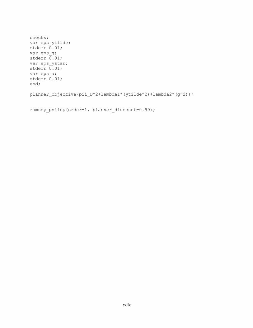
cxlix
shocks;
var eps_ytilde;
stderr 0.01;
var eps_g;
stderr 0.01;
var eps_ystar;
stderr 0.01;
var eps_a;
stderr 0.01;
end;
planner_objective(pii_D^2+lambda1*(ytilde^2)+lambda2*(g^2));
ramsey_policy(order=1, planner_discount=0.99);
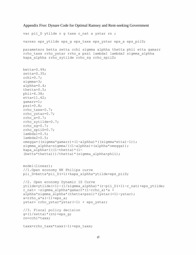
cl
Appendix Five: Dynare Code for Optimal Ramsey and Rent-seeking Government
var pii_D ytilde r g taxx r_nat a ystar rn ;
varexo eps_ytilde eps_g eps_taxx eps_ystar eps_a eps_piiD;
parameters betta zetta cchi sigmma alphha thetta phii etta gamarr
rrho_taxx rrho_ystar rrho_a pssi lambda1 lambda2 sigmma_alphha
kapa_alphha rrho_sytilde rrho_sg rrho_spiiD;
betta=0.99;
zetta=0.35;
cchi=0.7;
sigmma=3;
alphha=0.4;
thetta=0.5;
phii=4.38;
etta=11.42;
gamarr=1;
pssi=0.8;
rrho_taxx=0.7;
rrho_ystar=0.7;
rrho_a=0.7;
rrho_sytilde=0.7;
rrho_sg=0.7;
rrho_spiiD=0.7;
lambda1=0.5;
lambda2=0.5;
omegga=((sigmma*gamarr)+(1-alphha)*((sigmma*etta)-1));
sigmma_alphha=sigmma/((1-alphha)+(alphha*omegga));
kapa_alphha=(((1-thetta)*(1-
(betta*thetta)))/thetta)*(sigmma_alphha+phii);
model(linear);
//1.Open economy NK Philips curve
pii_D=betta*pii_D(+1)+kapa_alphha*ytilde+eps_piiD;
//2. Open economy Dynamic IS Curve
ytilde=ytilde(+1)-(1/sigmma_alphha)*(r-pii_D(+1)-r_nat)+eps_ytilde;
r_nat= -sigmma_alphha*gamarr*(1-rrho_a)*a +
alphha*sigmma_alphha*(thetta+pssi)*(ystar(+1)-ystar);
a=rrho_a*a(-1)+eps_a;
ystar= rrho_ystar*ystar(-1) + eps_ystar;
//3. Fiscal policy decision
g=(1/zetta)*(rn)+eps_g;
rn=cchi*taxx;
taxx=rrho_taxx*taxx(-1)+eps_taxx;

cli
end;
shocks;
var eps_ytilde;
stderr 0.01;
var eps_g;
stderr 0.01;
var eps_taxx;
stderr 0.01;
var eps_ystar;
stderr 0.01;
var eps_a;
stderr 0.01;
end;
planner_objective(pii_D^2+lambda1*(ytilde^2)+lambda2*(g^2));
ramsey_policy(order=1,periods=288, planner_discount=0.99);
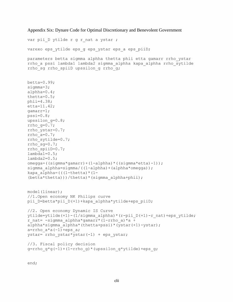
clii
Appendix Six: Dynare Code for Optimal Discretionary and Benevolent Government
var pii_D ytilde r g r_nat a ystar ;
varexo eps_ytilde eps_g eps_ystar eps_a eps_piiD;
parameters betta sigmma alphha thetta phii etta gamarr rrho_ystar
rrho_a pssi lambda1 lambda2 sigmma_alphha kapa_alphha rrho_sytilde
rrho_sg rrho_spiiD upssilon_g rrho_g;
betta=0.99;
sigmma=3;
alphha=0.4;
thetta=0.5;
phii=4.38;
etta=11.42;
gamarr=1;
pssi=0.8;
upssilon_g=0.8;
rrho_g=0.7;
rrho_ystar=0.7;
rrho_a=0.7;
rrho_sytilde=0.7;
rrho_sg=0.7;
rrho_spiiD=0.7;
lambda1=0.5;
lambda2=0.5;
omegga=((sigmma*gamarr)+(1-alphha)*((sigmma*etta)-1));
sigmma_alphha=sigmma/((1-alphha)+(alphha*omegga));
kapa_alphha=(((1-thetta)*(1-
(betta*thetta)))/thetta)*(sigmma_alphha+phii);
model(linear);
//1.Open economy NK Philips curve
pii_D=betta*pii_D(+1)+kapa_alphha*ytilde+eps_piiD;
//2. Open economy Dynamic IS Curve
ytilde=ytilde(+1)-(1/sigmma_alphha)*(r-pii_D(+1)-r_nat)+eps_ytilde;
r_nat= -sigmma_alphha*gamarr*(1-rrho_a)*a +
alphha*sigmma_alphha*(thetta+pssi)*(ystar(+1)-ystar);
a=rrho_a*a(-1)+eps_a;
ystar= rrho_ystar*ystar(-1) + eps_ystar;
//3. Fiscal policy decision
g=rrho_g*g(-1)+(1-rrho_g)*(upssilon_g*ytilde)+eps_g;
end;
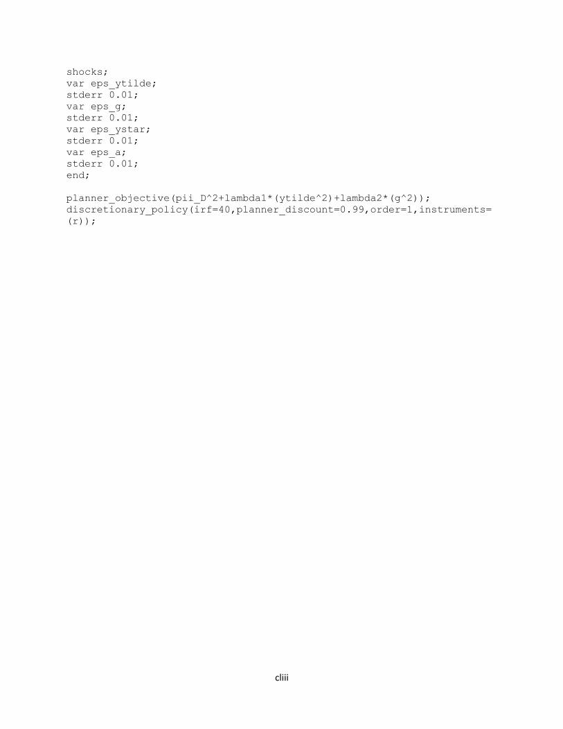
cliii
shocks;
var eps_ytilde;
stderr 0.01;
var eps_g;
stderr 0.01;
var eps_ystar;
stderr 0.01;
var eps_a;
stderr 0.01;
end;
planner_objective(pii_D^2+lambda1*(ytilde^2)+lambda2*(g^2));
discretionary_policy(irf=40,planner_discount=0.99,order=1,instruments=
(r));
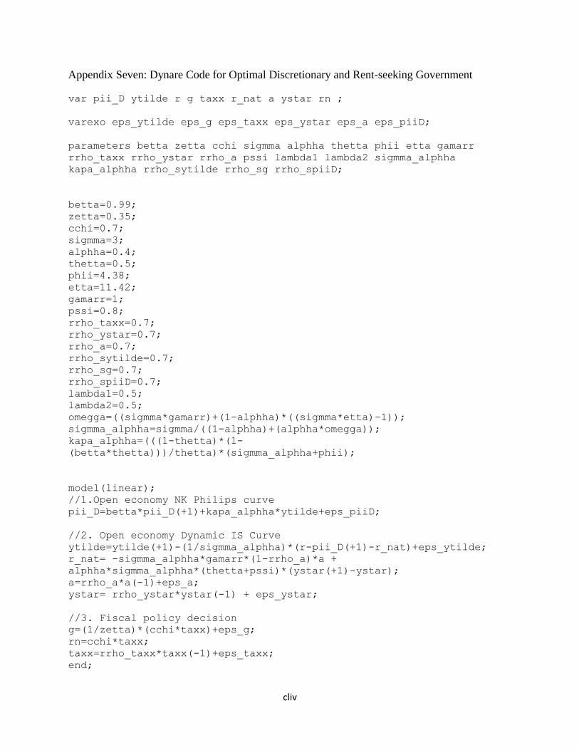
cliv
Appendix Seven: Dynare Code for Optimal Discretionary and Rent-seeking Government
var pii_D ytilde r g taxx r_nat a ystar rn ;
varexo eps_ytilde eps_g eps_taxx eps_ystar eps_a eps_piiD;
parameters betta zetta cchi sigmma alphha thetta phii etta gamarr
rrho_taxx rrho_ystar rrho_a pssi lambda1 lambda2 sigmma_alphha
kapa_alphha rrho_sytilde rrho_sg rrho_spiiD;
betta=0.99;
zetta=0.35;
cchi=0.7;
sigmma=3;
alphha=0.4;
thetta=0.5;
phii=4.38;
etta=11.42;
gamarr=1;
pssi=0.8;
rrho_taxx=0.7;
rrho_ystar=0.7;
rrho_a=0.7;
rrho_sytilde=0.7;
rrho_sg=0.7;
rrho_spiiD=0.7;
lambda1=0.5;
lambda2=0.5;
omegga=((sigmma*gamarr)+(1-alphha)*((sigmma*etta)-1));
sigmma_alphha=sigmma/((1-alphha)+(alphha*omegga));
kapa_alphha=(((1-thetta)*(1-
(betta*thetta)))/thetta)*(sigmma_alphha+phii);
model(linear);
//1.Open economy NK Philips curve
pii_D=betta*pii_D(+1)+kapa_alphha*ytilde+eps_piiD;
//2. Open economy Dynamic IS Curve
ytilde=ytilde(+1)-(1/sigmma_alphha)*(r-pii_D(+1)-r_nat)+eps_ytilde;
r_nat= -sigmma_alphha*gamarr*(1-rrho_a)*a +
alphha*sigmma_alphha*(thetta+pssi)*(ystar(+1)-ystar);
a=rrho_a*a(-1)+eps_a;
ystar= rrho_ystar*ystar(-1) + eps_ystar;
//3. Fiscal policy decision
g=(1/zetta)*(cchi*taxx)+eps_g;
rn=cchi*taxx;
taxx=rrho_taxx*taxx(-1)+eps_taxx;
end;
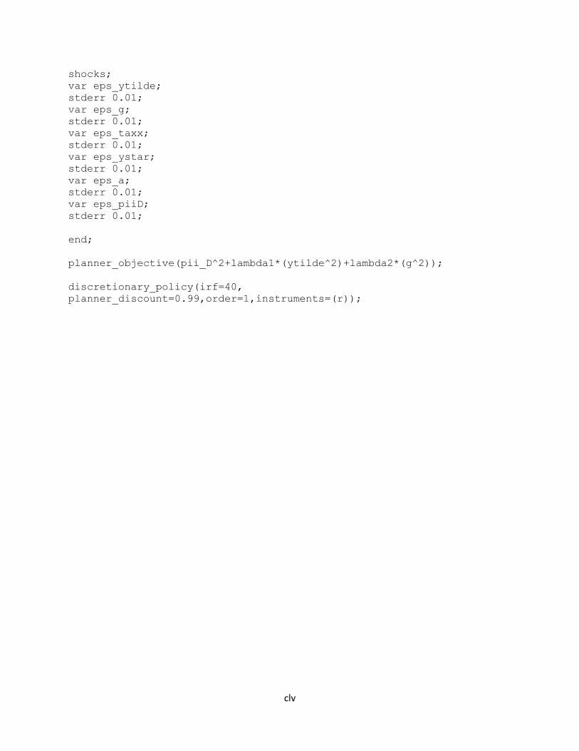
clv
shocks;
var eps_ytilde;
stderr 0.01;
var eps_g;
stderr 0.01;
var eps_taxx;
stderr 0.01;
var eps_ystar;
stderr 0.01;
var eps_a;
stderr 0.01;
var eps_piiD;
stderr 0.01;
end;
planner_objective(pii_D^2+lambda1*(ytilde^2)+lambda2*(g^2));
discretionary_policy(irf=40,
planner_discount=0.99,order=1,instruments=(r));
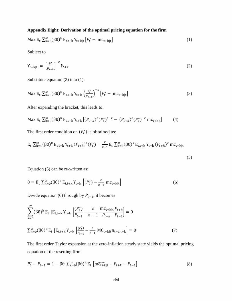
clvi
Appendix Eight: Derivation of the optimal pricing equation for the firm
Max Et ∑ (βθ)k∞k=0 Et,t+k Yt+k|t [𝑃𝑡
∗ − mct+k|t] (1)
Subject to
Yt+k|t = [𝑃𝑡
∗
𝑃𝑡+𝑘]
−𝜀
𝑌𝑡+𝑘 (2)
Substitute equation (2) into (1):
Max Et ∑ (βθ)k∞k=0 Et,t+k Yt+k (
𝑃𝑡∗
𝑃𝑡+𝑘)
−𝜀
[𝑃𝑡∗ − mct+k|t] (3)
After expanding the bracket, this leads to:
Max Et ∑ (βθ)k∞k=0 Et,t+k Yt+k [(𝑃𝑡+𝑘)𝜀(𝑃𝑡
∗)1−ε − (𝑃𝑡+𝑘)𝜀(𝑃𝑡∗)−ε mct+k|t] (4)
The first order condition on (𝑃𝑡∗) is obtained as:
Et ∑ (βθ)k∞k=0 Et,t+k Yt+k (𝑃𝑡+𝑘)𝜀(𝑃𝑡
∗) =ε
ε−1Et ∑ (βθ)k∞
k=0 Et,t+k Yt+k (𝑃𝑡+𝑘)𝜀 mct+k|t
(5)
Equation (5) can be re-written as:
0 = Et ∑ (βθ)k∞k=0 Et,t+k Yt+k [(𝑃𝑡
∗) −ε
ε−1 mct+k|t] (6)
Divide equation (6) through by 𝑃𝑡−1, it becomes
∑(βθ)k Et
∞
k=0
[Et,t+k Yt+k [(𝑃𝑡
∗)
𝑃𝑡−1−
ε
ε − 1
mct+k|t
𝑃𝑡+𝑘
𝑃𝑡+𝑘
𝑃𝑡−1] = 0
∑ (βθ)k Et ∞k=0 [Et,t+k Yt+k [
(𝑃𝑡∗)
𝑃𝑡−1−
ε
ε−1 MCt+k|tπt−1,t+k] = 0 (7)
The first order Taylor expansion at the zero-inflation steady state yields the optimal pricing
equation of the resetting firm:
𝑃𝑡∗ − 𝑃𝑡−1 = 1 − βθ ∑ (βθ)k Et
∞k=0 [mct+k|t + 𝑃𝑡+𝑘 − 𝑃𝑡−1] (8)

clvii
Where mct+k|t = mct+k|t − mc
Equation (8) can be re-arranged and re-written as:
𝑃𝑡∗ = 𝜇 + (1 − βθ) ∑ (βθ)k Et
∞k=0 [mct+k|t + 𝑃𝑡+𝑘] (9)
Where,
𝜇 = −𝑚𝑐 ≡ log휀
휀 − 1
From equation (9), it can be deduced that firms set a price according to the desired mark-up over
a weighted average of expected marginal cost

clviii
Appendix Nine: Prior-Posterior Plot

clix