Embed Size (px)
Citation preview
Name:
Department of Physics
First Year
Laboratory Scripts
MODULE I
2008/2009
October 2008

Department of Physics
1st year Laboratory
Module 1
Introduction to Experimental Procedures and Errors
Autumn 2008
Contents
Errors I - Introduction to Measurement Error ................................................................... 3 Errors II – Gaussian Distributions - The Dartboard. ....................................................... 15 Errors III – The Simple Pendulum.................................................................................. 19 Errors IV - Measurement of Time Intervals .................................................................... 20
3
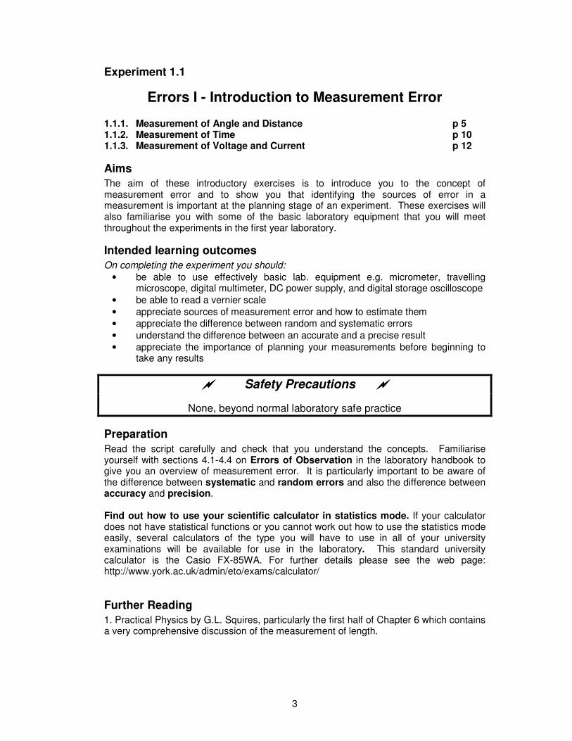
Experiment 1.1
Errors I - Introduction to Measurement Error
1.1.1. Measurement of Angle and Distance p 5 1.1.2. Measurement of Time p 10 1.1.3. Measurement of Voltage and Current p 12
Aims
The aim of these introductory exercises is to introduce you to the concept of measurement error and to show you that identifying the sources of error in a measurement is important at the planning stage of an experiment. These exercises will also familiarise you with some of the basic laboratory equipment that you will meet throughout the experiments in the first year laboratory.
Intended learning outcomes
On completing the experiment you should:
• be able to use effectively basic lab. equipment e.g. micrometer, travelling microscope, digital multimeter, DC power supply, and digital storage oscilloscope
• be able to read a vernier scale
• appreciate sources of measurement error and how to estimate them
• appreciate the difference between random and systematic errors
• understand the difference between an accurate and a precise result
• appreciate the importance of planning your measurements before beginning to take any results
Safety Precautions
None, beyond normal laboratory safe practice
Preparation
Read the script carefully and check that you understand the concepts. Familiarise yourself with sections 4.1-4.4 on Errors of Observation in the laboratory handbook to give you an overview of measurement error. It is particularly important to be aware of the difference between systematic and random errors and also the difference between accuracy and precision. Find out how to use your scientific calculator in statistics mode. If your calculator does not have statistical functions or you cannot work out how to use the statistics mode easily, several calculators of the type you will have to use in all of your university examinations will be available for use in the laboratory. This standard university calculator is the Casio FX-85WA. For further details please see the web page: http://www.york.ac.uk/admin/eto/exams/calculator/
Further Reading
1. Practical Physics by G.L. Squires, particularly the first half of Chapter 6 which contains a very comprehensive discussion of the measurement of length.

4
Introduction
Overall these introductory exercises aim to demonstrate the sort of critical approach to experimental work that we would like you to develop over the next year as well as familiarising you with some of the equipment that you will use in later experiments. This first session in the lab. will consist of a series of 3 exercises of approx. 1 hour duration which have been designed to get you thinking about some useful methods of measuring basic quantities such as length, time, angle, voltage and current. Your aims in each of the exercises are to:
a) develop a method of measuring each quantity as precisely or reproducibly as possible.
b) obtain an accurate measurement by minimising any systematic errors associated with each measuring device.
Over the course of the next 3 (or 4) years of your degree, you will handle many different instruments and there would be no time for investigating interesting physics if we spent time training you in the detailed use of each individual piece of equipment. Instead what we intend to do is to train you in the use of instruments in general and the approach you should adopt when handling any piece of equipment. Therefore the scripts for each exercise are not designed to provide step-by-step instructions in how to do the measurement but instead a demonstrator will lead you or your group through each task and discuss with you the ideas you need to think about before making any measurements. The purpose is to demonstrate to you that a good experimental physicist spends a lot of time thinking about how best to set about measuring the quantity of interest before touching any equipment. Incidentally these concepts are also just as important to theoretical and computational physicists, maths/physicists as many of the general principles of measurement and errors apply to theoretical modelling. Remember to keep a record of what you have done in your laboratory notebook as you go along. It is important to make notes about the ideas you and your group have in the discussions with the demonstrator as well as the results of your actual measurements. As well as obtaining a value for the quantity you are asked to measure in each exercise, you will be expected to give an estimate of the expected error in your measurement. Your demonstrator will help you to determine the appropriate error in your measured value. In most of the exercises your aim is to minimise both the systematic and random errors as much as you can.
Timetable of Events
Time Activity 1 Activity 2 Activity 3
12.15 Talk: Introduction to Laboratory Programme
12.45 Lunch 1.30 Talk: Introduction to Errors
2.00 Angle & Distance Time V & I 2.55 Break
3.20 Time V & I Angle & Distance 4.15 V & I Angle & Distance Time 5:10 Finish

5
1.1.1 Measurement of Angle and Distance
Measurement of Angle
In this exercise, you are asked to use the spectrometer as a surveyor’s theodolite in order to determine the distance of the spectrometer to the window. The aim of this exercise is to familiarise you with the measurement of angle using a vernier scale (see box for principles of a vernier scale).
Apparatus
You are provided with a metre ruler and a spectrometer. You may only use the ruler to measure the width of the window NOT the distance of the spectrometer from the window. Once you have calculated the distance, only then can you (if time permits) use an appropriate tape measure to check the distance you have calculated.
The Spectrometer
The spectrometer you will use, which is shown schematically in Figure 1.1, consists of three parts:
• The collimator - this is fixed in direction and has a variable width input slit and a lens which can be moved with the focusing knob. You will not be using the collimator in this exercise.
• The telescope - this has an objective lens and an eyepiece which can both be moved for focusing. It is free to rotate and has a Vernier scale attached so that the angular position can be measured accurately.
• The table - this is a flat table with a grating mounting screwed onto it. The table can be rotated independently of the telescope and it too has a Vernier scale attached. The height and tilt of the table can be adjusted.
CollimatorTelescope
TableVernier scale
Crosswires
LightSource Lens
Objective Lens
Eyepiece
Figure 1.1 Schematic Diagram of the Spectrometer
Both the table and telescope have locking screws as well as fine adjustment mechanisms. If the locking screw for the telescope is freed the telescope can be rotated by hand to any setting. If the locking screw is tightened the telescope can be moved precisely by means of the adjustment knob located close to the locking screw. Similar adjustments apply to the table rotation.
Focussing the Telescope
Look through the telescope and rotate the focusing screw until a distant object (the window in this case) is roughly in focus. Move the position of the eyepiece until the cross-wires are sharply focussed. Now make fine adjustments to the focussing screw until the distant object and the cross-wires are both sharply in focus and there is no parallax between the images. You may need to make successive small adjustments to the eyepiece and objective lens to achieve this.
6
Reading the Vernier Scale
The Vernier scale for angular measurement on the spectrometers works in a manner described in the appendix to this experiment which you should read before continuing.
The Experiment
In your group, and with your demonstrator as well, discuss how you are going to use the spectrometer to determine the distance of the mark on the laboratory bench from the window. Consider the following points:
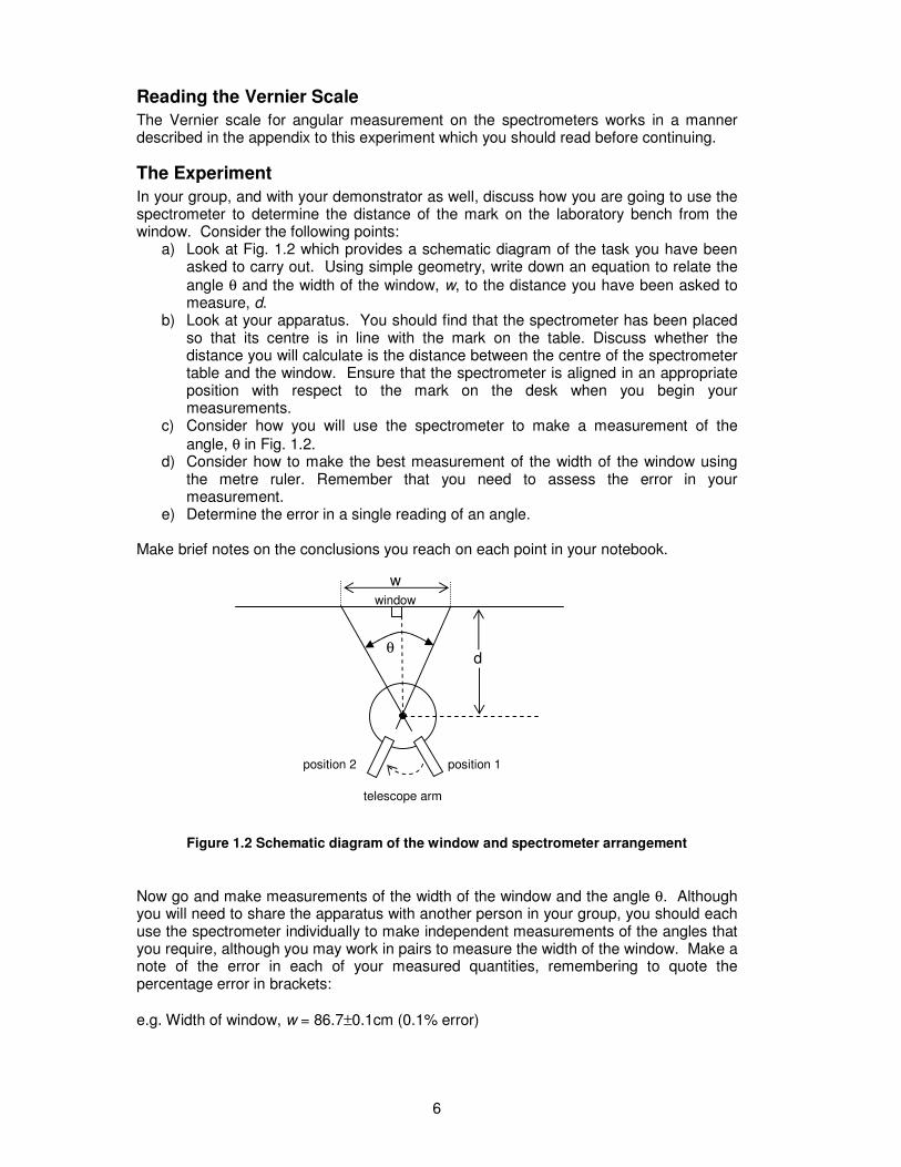
a) Look at Fig. 1.2 which provides a schematic diagram of the task you have been asked to carry out. Using simple geometry, write down an equation to relate the
angle θ and the width of the window, w, to the distance you have been asked to measure, d.
b) Look at your apparatus. You should find that the spectrometer has been placed so that its centre is in line with the mark on the table. Discuss whether the distance you will calculate is the distance between the centre of the spectrometer table and the window. Ensure that the spectrometer is aligned in an appropriate position with respect to the mark on the desk when you begin your measurements.
c) Consider how you will use the spectrometer to make a measurement of the
angle, θ in Fig. 1.2. d) Consider how to make the best measurement of the width of the window using
the metre ruler. Remember that you need to assess the error in your measurement.
e) Determine the error in a single reading of an angle. Make brief notes on the conclusions you reach on each point in your notebook. window
position 2 position 1
telescope arm
Figure 1.2 Schematic diagram of the window and spectrometer arrangement
Now go and make measurements of the width of the window and the angle θ. Although you will need to share the apparatus with another person in your group, you should each use the spectrometer individually to make independent measurements of the angles that you require, although you may work in pairs to measure the width of the window. Make a note of the error in each of your measured quantities, remembering to quote the percentage error in brackets:
e.g. Width of window, w = 86.7±0.1cm (0.1% error)
θ d
w
7
Analysis of Results
In order to calculate the error in the final result, it is necessary to combine the errors from your individual quantities in some way. You will learn more about this later in the introductory module so for the moment we will simply quote the formula that you can use to calculate the error (see laboratory handbook chapter 4). You should have worked out the distance, d using the following equation:
=
2tan2
θw
d (5)
Before we can work out the error in d, we need to work out the error in θ/2. To measure
θ, you measured the difference between two angles which we will call θ1 and θ2 and you should have errors in each quantity:
e.g. θ1 = 14.93 ± 0.01º so ∆θ1 = 0.01º
θ2 = 8.18 ± 0.01º so ∆θ2 = 0.01º
Therefore θ = θ1 - θ2 = 6.75º and the error in θ, ∆θ, is approximately 0.02º (by adding
together each error) so θ = 6.75±0.02º and therefore θ/2 = 3.38 ± 0.01º. We can work out the error in d using the expression:
2
2
2tan
2tan
∆+
∆=
∆θ
θ
w
w
d
d where θθθθ is in radians (6)
The fractional error in tan(θ/2) is a rather complicated expression and must be calculated
using θθθθ in radians:
( )2
sin2
cos2
2
2tan
22sec
21
2tan
2tan 2
θθ
θ
θ
θθ
θ
θ∆
=∆
=∆
(7)
However there is an alternative way to calculate the error in tan(θ/2) and this is the method we recommend that you use for this exercise:
1. Using equation 5, work out d using your measured values of w and θ/2.
e.g. using w = 86.7cm and θ/2 = 3.38º, d = 734 cm
2. Now work out d using your measured value of w and a value for θ/2 = measured
value of θ/2 + ∆θ/2:
e.g. using w = 86.7cm and θ/2 = 3.39º, d = 733 cm
3. So the error in d considering only the error in θ/2 = 734 - 733 = 1 cm.
4. Assume that the percentage error in d due to θ/2 equals the percentage error in
tan(θ/2) in equation 6.
e.g. % error in d = 100734
1× % = 0.1% so % error in tan(θ/2) = 0.1%
We can now work out the error in d by combining the errors in w and θ/2 using equation 6:
8
( ) ( ) %1.0%1.0%1.0
2tan
2tan
22
2
2
=+=
∆+
∆=
∆θ
θ
w
w
d
d
and ∆d = 0.1% of 734cm = ±2 cm
So the distance between the spectrometer and the window, d = 734 ±±±± 2 cm.
Discussion Questions
a) In your notebook, compare your measured value of the distance using the spectrometer to a value measured directly with a tape measure.
b) Measure the distance yourself with another person in your group (remember to include an estimate of the error in this measurement).
c) Do the two results agree within experimental error? If not, discuss reasons why (e.g. systematic errors, random errors too small).
Appendix on Reading Vernier Scales The vernier is a short supplementary scale alongside the main scale. It enables you to determine what fraction of main scale divisions the reading should be. The beginning of the vernier scale is its origin mark i.e. the zero line. It is this position on the main scale you are trying to read. The fraction between the two marks on the main scale where the zero line of the vernier lines up with the main scale is given by the number of division intervals on the vernier scale. Typically there are 10 vernier divisions, and therefore the vernier will read to 1/10th of a main scale division. There may be more divisions on some scales. For example, with 20 vernier divisions, a reading is given to 1/20th of a main scale division and this is the case for some spectrometers where the main scale divisions are 1/3 degree apart. If there are n vernier divisions, the vernier gives a reading to 1/nth of a main scale division. To read a vernier, notice that the zero line on the vernier usually lines up between two main scale divisions rather than exactly on one. Further along the vernier they come into coincidence with the main scale division lines and finally they go past them. See the diagram further down this page or look at the vernier scale on your instrument. To read the vernier, find the vernier division line that coincides exactly with a main scale division line. That vernier line gives the fraction of the main scale division you are looking for that needs to be added to the lower of the two readings on the main scale where the vernier zero line falls. Once you have learnt the secret, reading a vernier scale is easy if slightly time-consuming. It helps greatly when you are looking at finer scales to use a small magnifying glass often with an integral light. The larger the number of vernier divisions, the harder it is to judge the coincidence between scale lines. The vernier scale works because each vernier scale division is shorter than a
9
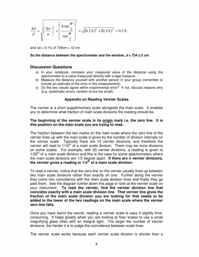
main scale division by one vernier division unit. For example, a vernier designed to read to 1/10th of a mm has divisions that are 1/10th mm shorter than the main scale divisions of 1 mm. If, as in the example below, the origin of the vernier scale starts 0.4 mm from a main scale division, it will take 4 vernier divisions before the vernier scale marks have dropped into exact alignment with a main scale mark. Hence the recipe for reading the vernier will produce the correct answer of 0.4 mm. Spend a little time to think about it.
3 4 5 6
0 10vernier scale
main scale
reading: 3.74 cm = 37.4 mm
Coincidence
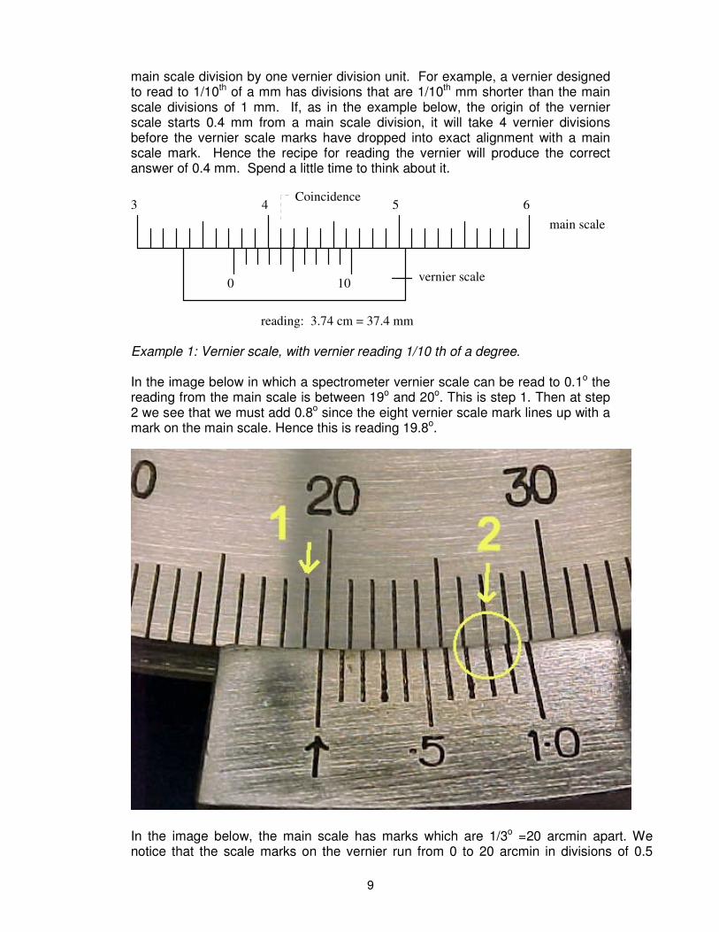
Example 1: Vernier scale, with vernier reading 1/10 th of a degree. In the image below in which a spectrometer vernier scale can be read to 0.1o the reading from the main scale is between 19o and 20o. This is step 1. Then at step 2 we see that we must add 0.8o since the eight vernier scale mark lines up with a mark on the main scale. Hence this is reading 19.8o.
In the image below, the main scale has marks which are 1/3o =20 arcmin apart. We notice that the scale marks on the vernier run from 0 to 20 arcmin in divisions of 0.5
10
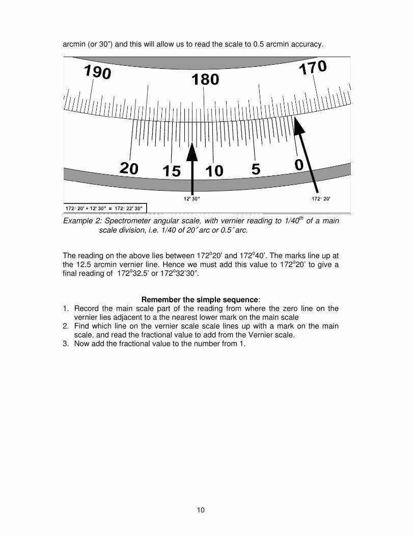
arcmin (or 30”) and this will allow us to read the scale to 0.5 arcmin accuracy.
Example 2: Spectrometer angular scale, with vernier reading to 1/40th of a main
scale division, i.e. 1/40 of 20′ arc or 0.5′ arc.
The reading on the above lies between 172o20’ and 172o40’. The marks line up at the 12.5 arcmin vernier line. Hence we must add this value to 172o20’ to give a final reading of 172o32.5’ or 172o32’30”.
Remember the simple sequence: 1. Record the main scale part of the reading from where the zero line on the
vernier lies adjacent to a the nearest lower mark on the main scale 2. Find which line on the vernier scale scale lines up with a mark on the main
scale, and read the fractional value to add from the Vernier scale. 3. Now add the fractional value to the number from 1.
11
1.1.2. Measurement of Time
In this exercise, your task is to measure time intervals of the order of milliseconds using a Digital Storage Oscilloscope (DSO). You are asked to measure the speed of sound in air using a pulsed echo technique.
Apparatus
The apparatus consists of an ultrasonic tape measure which provides a 45 kHz wave packet, or 'chirp', which is then reflected from a movable screen and is detected by two transducers mounted on a movable clamp stand. The transducers act as receivers, the first facing the tape measure to detect the outgoing chirp and the second facing the screen to measure the incoming pulse reflected from the screen. The time delay between emission and reception of the sound wave packet is measured with a Digital Storage Oscilloscope (DSO). The first transducer is connected to the Ch 1 input of the DSO and the second to Ch 2. When a transducer detects a chirp, it triggers the DSO and the wave packet is displayed on the screen. By measuring the time delay between the outgoing and incoming wave packets, the velocity of sound can be estimated if the distance of the reflecting screen is known. The distance can be estimated using a metre ruler. Remember that the actual distance travelled by the sound wave is twice the distance of the screen.
The Experiment
1. Ensure that the transducers are aligned with respect to the screen. Choose a suitable distance to begin your measurements (say 0.5m from the screen) and estimate the distance between the screen and the incoming transducer using the metre ruler. Note in your notebook your initial thoughts about the likely precision of your measurement.
2. Switch the DSO on (ON/OFF button is on the top of the box). If it is on already, switch it off for 1 second to clear any unusual previous settings and restore the scope to a default state. Once the DSO has powered up press any button to continue.
3. You will meet the DSO in more detail in later experiments this year so only very basic instructions on how to operate the ‘scope for this experiment will be given here. The DSO should power up in the default mode. Check the menu on the right hand side of the screen: Ch1 set to DC coupling, Probe set to 1X.
4. Begin with a practice run to see whether the DSO picks up a pulse on both Ch1 and Ch2. Press ‘Run’ (button on top right hand side of DSO) to begin. The DSO will trigger automatically when it detects a signal.
5. Hold the ultrasonic tape measure about 10-15cm away from the outgoing transducer and switch it on which should send out a pulse. The DSO should display a wavepacket on each Channel on the screen.
6. You can measure the distance between the two wave packets using the cursors on the DSO screen. Press the cursor menu button located on the panel of buttons on the top right hand side of the DSO. Move the cursors to the desired position using the cursor 1 and cursor 2 knobs (also Volt/div knobs) located on the main DSO control panel. The menu gives the position of cursor 1 and cursor 2 and delta gives the difference between the two cursor positions. As the wave packet has a rather complicated form it is difficult to measure the absolute time delay between emission and reception of the wave packet. Choose a prominent feature on the packet and measure the time delay.
7. Repeat the measurement a few times to see whether the time period you measure is consistent.
Once you have had a chance to look at the equipment, you need to consider how you can make the best measurements of the time interval between the pulses and the

12
distance the sound pulse travels. You are expected to make measurements of at least 5 different distances. Discuss within your group and with your demonstrator the following points:
a) what is the error in a single measurement of the distance travelled by the pulse (remember that this equals twice the distance from the clamp stand to the screen)? Consider how to make the most accurate and precise measurement of the distance.
b) what is the error in a single reading of the time interval? c) does the time interval vary when repeated readings are taken? d) Consider how to make the best measurement of the time interval for a particular
distance e) sources of systematic error - does each person in the group judge the time
interval to be the same in one particular scope trace? Make brief notes on the conclusions you reach on each point in your notebook. Now make the best measurements you can of the variation of time between the outgoing and incoming pulse at a range of distances. You should record your results in a table - a suggested format is shown here.
Distance /m
±error?
Total Distance /m
±error?
Time /ms
±error?
Mean time, t
/ms
∆t /ms
Vsound /ms-1
∆V /ms-1
Analysis of Results
The best value of your repeated readings of the time interval is given by the arithmetic mean (or average) value. If your repeated measurements of the time interval show a spread larger than the error in a single reading of the time then, to calculate the expected
error in your mean value, you need to calculate the standard deviation of your values, σ. Otherwise use the error in a single measurement as your error. You can use your scientific calculator to calculate both the mean and the standard deviation by putting your calculator into ‘statistics’ mode and enter each value of your reading as data into your calculator’s memory. You will need to consult your calculator’s manual to work out how to do this - a demonstrator may be able to help you if you are unsure. Alternatively you can calculate the standard deviation by hand (refer to section 4.4 of the lab handbook for an example of how to do this).
The best estimate of your measured value = mean of N readings = ∑x/N
The error in the mean = σ/√N Now calculate the speed of sound at each distance. Use each value to work out your best estimate of the speed of sound in air by calculating the mean of all your values. Work out the error in your mean as indicated above. Remember - only quote your error to 1 s.f. and quote your mean value to the same no of decimal places as your error. Also give the percentage error in brackets.
e.g. Mean value of speed of sound in air = 340 ± 20 ms-1 (6% error).
Discussion Question
In your notebook, compare your measured value of the speed of sound in air to the accepted value of 331ms-1 at S.T.P. Does your result agree within experimental error? If not, discuss reasons why (e.g. systematic errors, random errors too small).
13
1.1.3. Measurement of Voltage and Current
The input of an electrical meter is invariably resistive. Ideally meters should have an infinite input resistance when measuring potential difference, (p.d.) so that they draw no current from the circuit. Conversely, they should have vanishingly small input resistance when measuring current so that no p.d. is developed across them. In this exercise you will be using Digital Multimeters (DMM’s) to make voltage and current measurements, which come close to this ideal, but how close? In this exercise your task is to obtain a value of the resistance of an unknown resistor, Rx, in the circuit box provided by making measurements of voltage using the Thurlby DMM and measurements of current using another DMM and then applying Ohm’s Law.
Apparatus: Thurlby digital multimeter
Operation For DC operation leave the AC/DC push button switch in the 'out' position. For voltage measurement depress the button marked V; to measure resistance depress the button
marked Ω and to measure current depress both buttons V and Ω together. range: The range is chosen with the row of six push button switches; the meter reads directly in the unit indicated above the switch. For instance if the second button from the
left is depressed the meter reads up to 800 µA, 3200 Ω, or 3200 mV (3.2 Volts). Over-ranging: If the meter is out of range then the display will flash which indicates that you should increase the range setting. Accuracy The accuracy of the DMM is stated to be 0.05% which is +/– 5 in the last digit. You should use this value as an estimate of the error in a single reading of the voltage or current.
The Experiment
1. Connect the DC power supply (PS) to the input of the circuit box (marked ‘input’) so that it provides ~ 3 V which you can set using the dials on the power supply. Ask a demonstrator for help if you are unsure how to do this.
2. Referring to the schematic diagram of the circuit shown in Figure 3.1, connect the
meters to the circuit box as shown. Use the Thurlby DMM as your voltmeter, remembering to set it to measure voltage. Use the other DMM as your ammeter, set to read current. Seek the help of your demonstrator if you are unsure how to set this meter.
3. Now vary the p.d. across Rx by turning the potentiometer and measure the current as
a function of voltage across Rx. Use p.d. values in the range 0V – 3V. Draw a table in your notebook as shown below and use it to record your results:
14
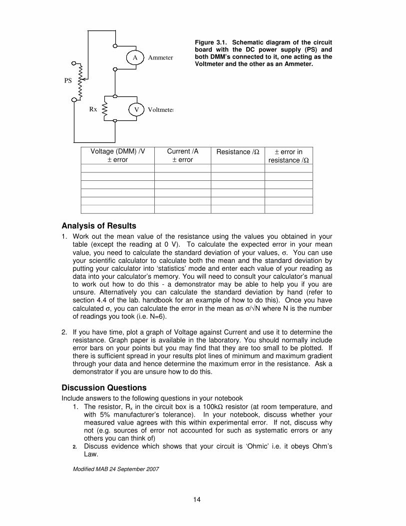
Figure 3.1. Schematic diagram of the circuit board with the DC power supply (PS) and both DMM’s connected to it, one acting as the Voltmeter and the other as an Ammeter.
Voltage (DMM) /V
± error
Current /A
± error Resistance /Ω ± error in
resistance /Ω
Analysis of Results
1. Work out the mean value of the resistance using the values you obtained in your table (except the reading at 0 V). To calculate the expected error in your mean
value, you need to calculate the standard deviation of your values, σ. You can use your scientific calculator to calculate both the mean and the standard deviation by putting your calculator into ‘statistics’ mode and enter each value of your reading as data into your calculator’s memory. You will need to consult your calculator’s manual to work out how to do this - a demonstrator may be able to help you if you are unsure. Alternatively you can calculate the standard deviation by hand (refer to section 4.4 of the lab. handbook for an example of how to do this). Once you have
calculated σ, you can calculate the error in the mean as σ/√N where N is the number of readings you took (i.e. N=6).
2. If you have time, plot a graph of Voltage against Current and use it to determine the
resistance. Graph paper is available in the laboratory. You should normally include error bars on your points but you may find that they are too small to be plotted. If there is sufficient spread in your results plot lines of minimum and maximum gradient through your data and hence determine the maximum error in the resistance. Ask a demonstrator if you are unsure how to do this.
Discussion Questions
Include answers to the following questions in your notebook
1. The resistor, Rx in the circuit box is a 100kΩ resistor (at room temperature, and with 5% manufacturer’s tolerance). In your notebook, discuss whether your measured value agrees with this within experimental error. If not, discuss why not (e.g. sources of error not accounted for such as systematic errors or any others you can think of)
2. Discuss evidence which shows that your circuit is ‘Ohmic’ i.e. it obeys Ohm’s Law.
Modified MAB 24 September 2007
Ammeter
Voltmeter Rx
A
V
PS
15
Experiment 1.2
Errors II – Gaussian Distributions - The Dartboard.
Aims
• To investigate the distribution of random errors and identify any systematic errors.
• To explore the statistical nature of random errors to quantify their effect on the error on the mean of a set of measurements.
Intended learning outcomes
On completing the experiment you should:
• understand what a Gaussian distribution is
• be able to calculate means, standard deviations and understand their relationship to repeated readings of a quantity and the Gaussian function
• be able to calculate the mean and uncertainty in the mean (standard error) for a set of data
• understand the difference between systematic and random errors
• appreciate how many repeated readings are required to generate a statistically significant Gaussian curve
Safety Precautions
Darts have sharp points and can cause injury if used carelessly. Before throwing darts, look around to check that nobody is in the way and that everyone around
you is aware that you are about to throw a dart.
Preparation
Read the script carefully and check that you understand the concepts. Remind yourself of the contents of section 4 of the Laboratory Handbook on Errors.
Further Reading
Further details regarding the Gaussian distribution can be found in ‘Practical Physics’ by G.L. Squires.
Introduction
Physical quantities observed in experiments usually have errors in the measurements which are random in nature. Random Errors vary arbitrarily from one observation to another and are likely to be positive or negative. For this reason, a single measurement of a quantity should not be relied upon. However repeated measurements of a single quantity often give a range of values and it is important to know how to obtain the best value from the measurements, and its reliability i.e. how close you think your ‘best’ value lies to the true value. In this experiment, you will build upon the ideas developed during the lecture on the Gaussian function before lunch. You will simulate repeated measurements of a single quantity by throwing darts at a central vertical strip on a dartboard and observing the spread in the attempts about the central strip. Parallel to the central strip (marked 0) are other strips of equal width (marked +1, +2, +3,etc to the right and -1, -2, -3 to the left). You will throw the darts in groups and then record the results. The number of the strip into which any darts falls is the observation for that particular throw. You should throw 20 sets of 5 darts .i.e. 100 throws in total.
16
The Experiment
Organising your notebook. You will need to organise your results table before commencing this experiment. In your lab. notebook set aside 20+ lines and use each line to record each set of 5 throws. This will take up about 2/3 of a page for your table. You will need a column for each of the strips marked on the dartboard (i.e. -10 to +10 so 21 columns) and also two slightly wider
columns, one headed ‘Mean of 5 throws’ and another headed ‘σ’ or ‘standard deviation’. You will also need an extra row at the bottom of the page to record the frequency, f, that each of the numbered strips was hit. Your demonstrator should be able to show you an example table if you are unsure. Organising your time. Due to the limited availability of space for dartboards, you will be divided into groups of 5 or 6 for this experiment. Each member of the group should throw a total of 20 sets of 5 darts in rotation. As you may have some time to wait between throwing your individual sets of darts, analyse your data after each set of five darts. You should calculate the mean and standard deviation using your calculator in its statistics mode. Remember to clear the memory after each calculation. Organising your throws. Standing on the marked base line, at a distance of 2m away from the board, throw the five darts, one-by-one, aiming at the zero strip to give a set of 5 readings and record the results. Try to throw the darts independently i.e. any one throw should not be influenced by the position of the dart previously thrown. If a dart falls out of the board before its position is recorded, throw it again; if it falls outside the numbered columns throw the dart again Continue throwing sets of 5 darts in rotation within your group until you have each thrown 20 sets of darts.
Analysis of Results
This section is much longer than a typical experiment that you will meet in the lab. because here the emphasis is on the statistical analysis. Make sure you record answers to the questions in bold in your notebook as you work through the analysis of your results. Complete the final row of the results table by counting up the total number of ‘hits’ for each of the numbered strips and enter it into the ‘frequency’ row at the bottom of your table. On a piece of graph paper, draw a histogram of your 100 observations. Remember to label your axes and to fix the graph paper into your lab notebook. If your throwing were subject to random errors, then the distribution represented by your histogram should be an approximation to a Gaussian (or Normal) distribution. The spread of your observations about the mean value is best represented by the standard
deviation, σ, which is the root mean square deviation of all the individual readings from the mean (see section 4.4 of the lab handbook):
∑ −= 2)(1
xxn
iσ (1)
Calculate the mean of 100 throws ( x ) and its standard deviation, σ using your calculator
in statistics mode. Refer to section 4.4 of the lab handbook or ask a demonstrator for assistance if you are not sure how to do this. Remember that strips to the left of 0 are negative. The mean of your observations should be quite close to 0, if not, there is a systematic error or bias in your throwing. You could adjust your values by renumbering
17
your strips but it is not necessary here. Make a note in your lab. book whether or not you have a bias in your throwing.
You will normally calculate σ using your calculator in statistics mode as above but in this
experiment, we will also calculate σ using equation 1 to help you understand the statistical meaning of the standard deviation. To do this, construct a table of 5 columns in your notebook, as follows (start your values of x from the largest negative value for which you have recorded a ‘hit): e.g. Mean value, x = -0.21
x x- x d2 = (x- x )2 f fd2
-8 -7.79 60.68 3 182.1
.. 8 Total =Sum of all fd2
You can calculate the standard deviation, σ, by rewriting equation 1 in terms of the final column of your table and the total number of throws, n=100:
)fd all of (Sum11
)(1 222
nfd
nxx
ni ==−= ∑∑σ (2)
If you haven’t made a mistake, this value of σ should be the same as the one you obtained using your calculator in statistics mode. If your values do not agree to 1 s.f., check your calculations. Mark on your histogram a vertical line corresponding to your value of the mean x and
label it accordingly. For a very large number of observations (n→∞), your histogram would fall on a smooth curve falling away evenly towards zero on either side of a central maximum situated at the mean value x . For a Gaussian distribution, ~68% of
observations should be within ±1σ of the mean and ~95% should be within ±2σ. Mark on your histogram vertical lines corresponding to these limits and find the fraction of your observations which are within these limits. Are your results consistent with what is expected for a Gaussian distribution?
If you were to throw another single dart, what can you say about where you would expect it to land? (Hint - Your histogram for 100 darts provides guidance as it represents the probability distribution of a single throw. In other words, assuming that your distribution were Gaussian, there is a 68% probability that a single throw will be
within ±σ of the mean and a 95% it will be within ±2σ. This is why we say that the
standard deviation, σσσσ, is the error associated with a single throw or measurement).
Now from the 20 sets of 5 observations, you have calculated 20 mean values, mx . The
mean of all these means gives you the mean of all 100 observations and in fact the mx ’s
themselves form a Gaussian distribution about the true mean. The true mean being that
which would be calculated if n→∞. Construct a table to show the distribution of the means to enable you to draw another histogram, superposed on your original histogram, which indicates the distribution of the means. Although 20 values is too small a number to show the form of the distribution very clearly, it should be clear that the spread of the values of the means is much smaller than the spread of the original values. We can conclude from this that finding the mean of even a few observations gives a value which has less error than a single observation. To test this, we use the standard
18
deviation σm of the 20 values of mx and use it to calculate σ
σ m . This generally should be
equal to n
1 where n is the number of observations leading to each mean (i.e. n=5 in
this case). Confirm in your notebook that the result agrees reasonably with the
theory. We can conclude from this that the precision of the mean improves as √√√√n the
number of readings e.g. a mean value of 9 readings is √9 or 3 times more precise than a single reading of the same quantity i.e. the error in the mean will be 3 times smaller.
Discussion Questions
You should include the answers to the following questions in your lab notebook:
1. Was your throwing ability (as measured by σ) constant throughout the experiment?
2. Suppose your skill were such that nearly every dart hit the zero strip. What effect
would this have on the analysis of the results and the uncertainty?
3. Discuss the validity of the following by picking out evidence from your results:
a. A single observation can be incorrect by an amount which you have no means of estimating unless other observations are made.
b. A set of repeating readings leads to a mean value in which you have more confidence than a single reading as it provides a means of estimating how reliable the mean value is.
Summary remarks
1. Normally there is a limit to the time available for repeating readings of a single value so small numbers of observations (not usually more than 10) have to suffice. In general try to take at least 5 readings if you can.
2. The best estimate of a measured value is the mean of n readings, x , and the
uncertainty or error in the mean, ∆x, is called the standard error = σσσσ/√√√√n where σ is the standard deviation.
3. Remember that the uncertainty in the standard deviation is larger with a smaller
number of readings and so the standard error in the mean is itself approximate. Therefore do not quote the standard error to an unrealistic precision.
4. As suggested in section 4.6 of the lab handbook, an estimate of the error in the mean value to 1 part in 4 is adequate so you can usually quote your estimate of the error to 1 significant figure. Quote your result to the same number of decimal places and quote the error as a percentage in brackets as follows:
e.g. Mean value of Young’s Modulus, E = (2.03 ± 0.02)*1011 Nm (1% error) Modified MAB 24 September 2007
19
Experiment 1.3
Errors III – The Simple Pendulum
Aims
• To understand the minimisations of errors in an experiment
• To discover how precisely you, as an observer, can measure time
• To analyse an expression to determine the error in a quotient
Intended learning outcomes
On completing the experiment you should:
• know how most precisely to use a stop watch.
• know how to calculate the period and error in a single oscillation of a pendulum.
• be able to estimate the acceleration due to gravity and its associated error.
• appreciate that the period of oscillation depends upon the amplitude.
Safety Precautions
Much as I have tried I cannot discover any hazards in this experiment!
Preparation
Read the script carefully and check that you understand the concepts. Further details regarding the simple pendulum can be found in almost any elementary book on mechanics. Refresh yourself of Section 4 of the laboratory handbook. Look up the value of the acceleration due to gravity ‘g’ in a data book such as Kaye and
Laby (available in the lab.) and note it in your lab. notebook.
Introduction
This experiment focuses your attention on the strategy of minimising error in simple measurements. In order to measure the acceleration due to gravity you will need to measure the length of a simple pendulum and also the time period of the oscillation. However before adopting a particular strategy you will have to discover how accurately you can use a stop watch and a metre rule because this will determine how many oscillations you will need to observe in order to make the error in your time and length measurements approximately the same.
Theory
The period T of a simple pendulum of length l is:
T = 2g
lπ
Where g is the acceleration due to gravity
Rearranging the equation we have
2
24
T
lg
π= (1)
20
Thus the fractional error in g is
2/122
2
∆+
∆=
∆
T
T
l
l
g
g (2)
Check for yourself how to arrive at eqn 2. As you require the fractional error in both l and t to be approximately the same you can see that you will need the fractional error in the time to be half that in the length.
PRELIMINARY INVESTIGATION Set up the simple pendulum by clamping the string in the jaws of the retort clamp so that it swings over the surface of the bench and is as long as practicable. Fix a piece of paper to the bench and mark the centre position of the pendulum and two lines at +/- 5 cm. Now:
• Set the pendulum swinging from one of the 5 cm lines and determine the time for five complete oscillations, counting zero at the first transit from which you start your measurement.
• Count your oscillations and stop the timer at the tenth transit (i.e. five complete oscillations) of your zero line.
• Repeat this measurement five times, taking care to start the pendulum at the
same place each time. From this, estimate the error t∆ in your measurement of
time for five oscillations. (If you anticipate the times of transit then you should be able to measure the time to about 0.01 sec.)
The reason for this procedure is that the period of a simple pendulum depends upon the amplitude. If your timing accuracy is high then the variation of time with amplitude can become an important effect. Thus it is important to make an estimate of a reasonable number of oscillations for the measurement. To do this, you will estimate the number of oscillations required to ensure that the errors associated with measurements of time and length contribute equally to the total error in g. If we define T (and T∆ ) to be the time (and error) for one oscillation, and t (and t∆ ) to be the time (and error) for n oscillations, then by equating the fractional errors from l and T we get:
∆=
∆
T
T
l
l2
But t = nT where n is the number of oscillations and T is the period.
Thus t∆ = n T∆ or n
tT
∆=∆
∴
∆
=
∆
T
t
nl
l 2
Or the number of swings n =
∆
∆
l
t
T
l2
As an example if l = 600 mm, T=1.5 sec, t∆ = 0.01 sec and l∆ = 1 mm => n = 8.
Thus 8 full swings is reasonable in this case (you should use your own measurements). If more swings are used, the increased accuracy of T will not help as the error in length is now the dominant error. THE EXPERIMENT Once you have determined the number of swings n you will use in your experiment make five sets of measurements of n oscillations and calculate the mean and standard deviation of T. Make five independent measurements of the pendulum length and find its mean and standard deviation.
21
Analysis Now calculate the acceleration of gravity g and its error from equations (1) and (2) and
compare your value with that you found in Kaye and Laby. Improving the accuracy In order to improve the timing accuracy of the experiment you could increase the number of swings. However this would be pointless unless you can improve the precision with which you measure the length. To improve the measurement of length use the two rectangular plastic discs to hold the string in the retort clamp and measure the length with this new arrangement. You should now be able to measure l more accurately and thus it is worth increasing the number of oscillations. With the improved precision recalculate the number of oscillations you require to make the errors comparable and repeat the above experiment. Determine g and its error again. If you have managed to use the stop watch to the limit of its precision you will find that you can observe the increase in time period of the pendulum with amplitude. Increase the starting displacement to 10 cm and measure the period of n swings.
Discussion Questions
1. For the increased amplitude measurements, is the result significant?
2. Is there any need to correct your original result for g for the finite amplitude of
the pendulum? Is the difference larger than the error? 3. What are the systematic errors in this experiment you have ignored?
Further reading
G.L. Squires Practical Physics Modified MAB 24 September 2007 .
20
Experiment 1.4
Errors IV - Measurement of Time Intervals
Aims
• To introduce you to the measurement of microsecond time intervals by measuring the contact time of a bouncing ball.
• To use a digital storage oscilloscope (DSO) to capture transient pulses.
• To estimate and combine errors.
• To introduce the Easyplot program for plotting and curve fitting data.
• To investigate the contact time as a function of impact velocity.
Intended learning outcomes
On completing the experiment you should:
• be able to use a DSO to capture short pulses and measure their duration with consideration of errors.
• have estimated the contact time and the depth of penetration of a bouncing ball including an estimate of the systematic and random errors.
• be able to enter data into Easyplot, plot graphs with error bars, and use the linear fitting to determine the gradient, intercept, and errors on these.
Safety Precautions
None over and above normal laboratory safe practices
Preparation
Read section 4 in the laboratory handbook on Errors of Observation, and section 6 on Easyplot.
Introduction and Theory
The contact time and the depth of penetration of a bouncing ball
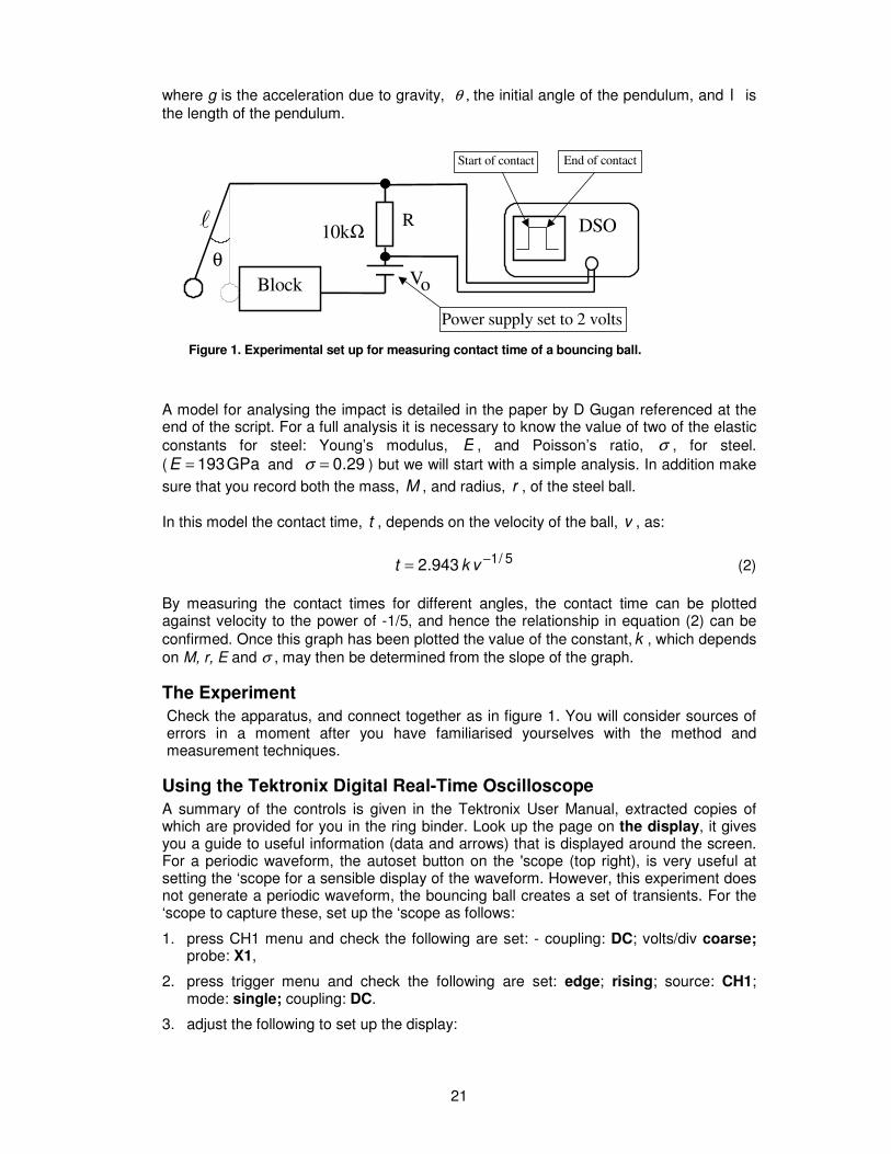
This experiment measures the time interval during which a bouncing steel ball is in contact with a steel block and from this the depth of penetration can be estimated. From figure 1 you will see that the steel ball and block act as an electrical switch and
during contact current flows around the circuit such that the potential difference, Vo,
appears across the resistor, R. By setting up the ‘scope appropriately, the onset of contact triggers the oscilloscope and the period during which the ball and block are in contact can be measured directly from the length of the trace displayed on the ‘scope
time axis at Vo. In order to estimate the depth of penetration you will need the impact
velocity of the sphere and this can be obtained from knowledge of the angle and the length of the suspension wire. It can be shown, by equating potential energy at the start of the swing to kinetic energy at the bottom of the swing, that the velocity, v, of the pendulum at the bottom of its swing, which is the point of impact, is given by:
v = (2g l (1-cosθ))½ (1)
21
where g is the acceleration due to gravity, θ , the initial angle of the pendulum, and l is
the length of the pendulum.
A model for analysing the impact is detailed in the paper by D Gugan referenced at the end of the script. For a full analysis it is necessary to know the value of two of the elastic
constants for steel: Young’s modulus, E , and Poisson’s ratio, σ , for steel.
( GPa193=E and 29.0=σ ) but we will start with a simple analysis. In addition make
sure that you record both the mass, M , and radius, r , of the steel ball.
In this model the contact time, t , depends on the velocity of the ball, v , as:
5/1943.2 −= vkt (2)
By measuring the contact times for different angles, the contact time can be plotted against velocity to the power of -1/5, and hence the relationship in equation (2) can be
confirmed. Once this graph has been plotted the value of the constant,k , which depends
on M, r, E and σ , may then be determined from the slope of the graph.
The Experiment
Check the apparatus, and connect together as in figure 1. You will consider sources of errors in a moment after you have familiarised yourselves with the method and measurement techniques.
Using the Tektronix Digital Real-Time Oscilloscope
A summary of the controls is given in the Tektronix User Manual, extracted copies of which are provided for you in the ring binder. Look up the page on the display, it gives you a guide to useful information (data and arrows) that is displayed around the screen. For a periodic waveform, the autoset button on the 'scope (top right), is very useful at setting the ‘scope for a sensible display of the waveform. However, this experiment does not generate a periodic waveform, the bouncing ball creates a set of transients. For the ‘scope to capture these, set up the ‘scope as follows:
1. press CH1 menu and check the following are set: - coupling: DC; volts/div coarse; probe: X1,
2. press trigger menu and check the following are set: edge; rising; source: CH1; mode: single; coupling: DC.
3. adjust the following to set up the display:
Block
DSO 10k Ω
V o
θ
l R
Figure 1. Experimental set up for measuring contact time of a bouncing ball.
Power supply set to 2 volts
Start of contact End of contact
22
• trigger level (arrow on right hand side of display), turn trigger level control until trigger level is about 1 V;
• turn time base control to either 10 or 25 µµµµs/div (will depend on exact contact time). You can move the trigger position (arrow at top of display) to the left by turning the horizontal position control. This will give you more space to display the contact pulse;
• turn CH1 sensitivity control to 500 mV/div and adjust ch1 position to be in the lower half of the display.
4. to set the ‘scope ready to capture the pulse at contact, press the run/stop button (at top of the display it should say ‘ready’ as opposed to ‘stop’ when it has captured a signal). The ball will bounce several times, but the ‘scope will capture only the first contact pulse.
5. now practice bouncing the ball to see if the ‘scope captures the transient contact pulse. You will need to press run/stop each time to ‘ready’ the ‘scope to capture the pulse when you are about to release the ball. Note, the display does not clear when ‘ready’ to capture the next pulse, but is updated when the new pulse is captured.
6. you can determine the contact time from the length of the trace on the ‘scope display by using the cursors. Press cursor button and select ‘time’ from the menu. The ch1 and ch2 position controls now move two cursors which you can position one on the start of contact pulse and one on the end of the contact pulse. The time difference is then displayed on the menu at the right hand side of the display.
Sources of error
In order to consider how to make the best measurements with this apparatus, you will need to consider sources of error.
• What sources of systematic errors might there be in this experiment? • What sources of random errors are there?
• How will you minimise both of these in order to obtain precise and accurate results?
Think and plan for these now.
Laboratory notebooks
You must now start writing things down in your laboratory notebook. The experiment is at the point where your input matters to the outcome, and it is therefore important to record all your actions and thoughts.
• Write down your ideas for the sources of systematic and random errors in your laboratory notebook, then discuss them with a demonstrator before proceeding. After your discussion:
• write down a plan of how you will carry out the experiment including how the systematic and random errors you listed above will be minimised.
Make any adjustments to the apparatus in the light of your plans, and record these adjustments in your notebook, including any measurements taken (e.g. length of pendulum) together with an estimate of the measurement error. You should now draw up a table into which you will directly record the results. How many columns? - Don’t forget columns for the errors and derived results (e.g. velocity, penetration depth). Check with a demonstrator. Now measure the contact times for different angles.
23
Analysis of Results
Calculate the best value of any repeated measurements by determining the average value, and the error in that average by using your calculator to calculate the standard deviation and hence the standard error (section 4.4 in errors of observation). Enter these into your results table together with all the derived results, using equation (1) to calculate the velocity of the ball at impact and also determine the contact time in each case. The error in the velocity can be found as follows using formula given in section 4.5 and table 4.1 of errors of observation. To see how to proceed let’s break down the velocity equation into identifiable steps to which we can apply the various formula for combining
errors. To do this we substitute w = cosθ, u = 1-w, and s = 2g l u. Now the velocity
equation is v = √s.
Using the power formula for combining errors: s
s
v
v ∆=
∆5.0 .
Using the product formula for combining errors:
222
∆+
∆+
∆=
∆u
u
g
g
s
s
l
l.
Note: error in g is negligible, and can be ignored.
Using the difference formula for combining errors: wu ∆=∆ . Note: there is no error in the
constant ‘1’!
Using the function formula for combining errors: θθ sin∆=∆w (θ in radians, remember).
The fractional error in u is therefore: θθθ
cos1
sin
−∆
=∆u
u
Thus the final error formula for the velocity becomes:
22
cos1
sin5.0
−∆
+
∆=
∆θθθ
l
l
v
v (3)
Finally, we need to determine an error in 5
1−
v . From the power law, we find that the
fractional error in 5
1−
v is given by v
v∆5
1
Calculate all the errors and plot a graph for equation (2) – using Easyplot (see below) or Mike’s Excel sheet – of the contact time against the velocity to the power -1/5. From the graph confirm that the straight line fit represents the data and find the value of
k from the slope.
The penetration depth,d , depends on the impact velocity, v , according to the equation:
5/4kvd = (4)
where the constant k was found from the slope of your graph. If you write a formal
report on this you should refer to Gugan’s paper and confirm that the value of k agrees with that calculated from the known values of the elastic constants of steel.
24
Easyplot
The following notes make reference to section 6 of the laboratory handbook on Easyplot. You will need to enter your data directly into Easyplot (section 6.1.1.2 Entering data directly), making sure the correct assignment for the columns are used. Click on ‘plot’ to generate graph. A few things to check that are set up correctly:
1. If error bars are not displayed refer to section 6.1.1.2 to see what to do
2. In ‘preferences’ in the ‘file’ menu, make sure ‘error bars’ are set to ‘half of entire bar’
(this assumes your error ∆x represents half the error bar, i.e. your error is ±∆x) and that the error is the ‘error value’ (not percentage or fractional error)
3. Also in ‘preferences’ select ‘CurveFit 1’ and check ‘uncertainties’ (otherwise the errors in the gradient and intercept will not be shown).
Now follow the instructions in section 6.1.5 Curve fitting to fit a straight line with gradient, intercept, error on gradient, and error on intercept shown.
Discussion Questions
You should include the answers to the following questions in your lab notebook:
1. Are the error bars significantly larger or smaller than the deviations of the points from a smooth line or curve?
2. How well does the graph that you have plotted confirm the relationship between contact time and impact speed?
3. What other graph could have been plotted as an alternative that would allow you to find the power dependence on velocity for the contact time, rather than assuming it was -1/5?
4. Would you expect the line to pass through the origin? Does it, within the error on the intercept? If not, suggest reasons why not?
5. What is the most significant source of error in your measurements, and how could this be reduced in future?
Further Reading
1) G.L. Squires, Practical Physics 2) “Inelastic Collision and the Hertz theory of impact”, D. Gugan, Am. J. Phys 68 (2000) 920-924 (or follow the link on the Year 1 Laboratory web page). Modified MAB/MDC 24 September 2007