First-Order Methods of Smooth Convex Optimization with Inexact Oracle. · First-Order Methods of Smooth Convex Optimization with Inexact Oracle. 3 on the availability and relative

Noname manuscript No.(will be inserted by the editor)

First-Order Methods of Smooth ConvexOptimization with Inexact Oracle.

Olivier Devolder ·Francois Glineur · Yurii Nesterov

the date of receipt and acceptance should be inserted later

Abstract We introduce the notion of inexact first-order oracle and analyzethe behaviour of several first-order methods of smooth convex optimizationused with such an oracle. This notion of inexact oracle naturally appears in thecontext of smoothing techniques, Moreau-Yosida regularization, AugmentedLagrangians and many other situations.

We derive complexity estimates for primal, dual and fast gradient methods,and study in particular their dependence on the accuracy of the oracle andthe desired accuracy of the objective function. We observe that the superiorityof fast gradient methods over the classical ones is no longer absolute when aninexact oracle is used. We prove that, contrary to simple gradient schemes,fast gradient methods must necessarily suffer from error accumulation.

Finally, we show that the notion of inexact oracle allows the applicationof first-order methods of smooth convex optimization to solve non-smooth orweakly smooth convex problems.

The first author is a F.R.S.-FNRS Research Fellow. This text presents research results ofthe Belgian Program on Interuniversity Poles of Attraction initiated by the Belgian State,Prime Minister’s Office, Science Policy Programming. The scientific responsibility rests withits authors.

O. DevolderUniversite catholique de Louvain, ICTEAM Institute, B-1348 Louvain-La-Neuve, Belgium;Universite catholique de Louvain, CORE, B-1348 Louvain-La-Neuve, Belgium.Tel.: +32-10-479422, Fax: +32-10-474301E-mail: [email protected]

F. GlineurUniversite catholique de Louvain, ICTEAM Institute, B-1348 Louvain-La-Neuve, Belgium;Universite catholique de Louvain, CORE, B-1348 Louvain-La-Neuve, Belgium.E-mail: [email protected]

Y. NesterovUniversite catholique de Louvain, ICTEAM Institute, B-1348 Louvain-La-Neuve, Belgium;Universite catholique de Louvain, CORE, B-1348 Louvain-La-Neuve, Belgium.E-mail: [email protected]

2 O. Devolder, F. Glineur and Yu. Nesterov

Keywords Smooth convex optimization, first-order methods, inexact oracle,gradient methods, fast gradient methods, complexity bounds.

Mathematics Subject Classification (2000) 90C06, 90C25, 90C60

1 Introduction

In large-scale convex optimization, first-order methods are methods of choicedue to their cheap iteration cost. When the objective function is assumed to besmooth, for example when its gradient is Lipschitz-continuous with constant L,the simplest numerical schemes to be considered are the gradient method andits variants. If accuracy ε is desired for the objective function, these methodsrequire O

(Lε

)iterations.

However, it is well-known that in the black-box framework [11], first-order

methods can achieve the lower complexity bound of O(√

Lε

)iterations. Such

optimal methods, called Fast Gradient Methods (FGM), have been developedfor various classes of problems since 1983 [12,13,14,15] and outperform the-oretically, and often in practice, the classical gradient methods. Interest intothese methods has been renewed recently with development of smoothing tech-niques for non-smooth convex problems (see [15,16,17,4]), where FGMs areused to minimize a smooth approximation of a non-smooth objective function.

Standard analysis of first-order methods assumes availability of exact first-order information. Namely, the oracle must provide at each given point theexact values of the function and its gradient. However, in many convex prob-lems, including those obtained by smoothing techniques, the objective func-tion and its gradient are computed by solving another auxiliary optimizationproblem. In practice, we are often only able to solve these subproblems approx-imately. Hence, in that context, numerical methods solving the outer problemare provided with inexact first-order information. This led us to investigatethe behavior of first-order methods working with an inexact oracle.

We introduce in Section 2 a new definition of inexact first-order oracleand list a few simple examples. In Section 3, we show how our concept isapplicable to situations when the inexact oracle is computed by an auxiliaryoptimization problem. In particular, we consider convex-concave saddle pointproblems, augmented Lagrangians, and Moreau-Yosida regularization.

In Sections 4 and 5, we consider classical (primal and dual) and fastgradient methods, designed for the class of convex functions with Lipschitz-continuous gradient. We obtain efficiency estimates when these methods areused with an inexact first-order oracle. We also study the link between desiredaccuracy for the objective function and necessary accuracy for the oracle. Weobserve that the superiority of the fast gradient methods over the classical onesis no longer absolute when an inexact oracle is used, because FGMs suffer fromerror accumulation. In particular, fast methods require first-order informationwith higher accuracy than standard gradient methods to obtain a solutionwith a given accuracy. Therefore, the choice between these methods depends

First-Order Methods of Smooth Convex Optimization with Inexact Oracle. 3

on the availability and relative cost of an inexact oracle at different levels ofaccuracy, as is explained in Section 6.

In Section 7, we compare our approach with other definitions of inexactoracle, as applied to the smoothed max-representable functions typically ob-tained by the smoothing techniques [3,1]. We show that our definition can givebetter complexity results.

Our definition of inexact oracle is applicable to non-smooth and weaklysmooth convex problems. Section 8 shows how to apply first-order methodsdesigned for smooth convex optimization to functions with a weaker level ofsmoothness. For that, we show that (exact) first-order information for a non-smooth problem, such as subgradients, can be viewed as an inexact oracle,so that the methods of Sections 4 and 5 can be applied. We obtain in thisway “universal” first-order methods possessing optimal rates of convergencefor objective functions with different level of smoothness. We also prove lowerbounds on the rate of error accumulation for any first-order method using aninexact oracle, which shows that all methods discussed in this paper have thelowest possible rate of error accumulation. In particular, it appears that whileslower standard gradient methods are able to maintain an error comparable tothe oracle accuracy, any optimal method must suffer from error accumulation.

2 Inexact first-order oracle

2.1 Motivation and definition

We consider the following convex optimization problem:

f∗ = minx∈Q

f(x), (1)

where Q is a closed convex set in a finite-dimensional space E, and functionf is convex on Q. Space E is endowed with the norm ‖·‖E and E∗, the dualspace of E, with the dual norm ‖g‖∗E = supy∈E|〈g, y〉| : ‖y‖E ≤ 1 where 〈., .〉denotes the dual pairing. For example, by fixing a positive definite self-adjointoperator B : E → E∗, we can define the following Euclidean norms:

‖h‖E = ‖h‖2 = 〈Bh, h〉 ∀h ∈ E

‖s‖∗E = ‖s‖∗2 = 〈s,B−1s〉 ∀s ∈ E∗.

We assume that problem (1) is solvable with optimal solution x∗.Consider F 1,1

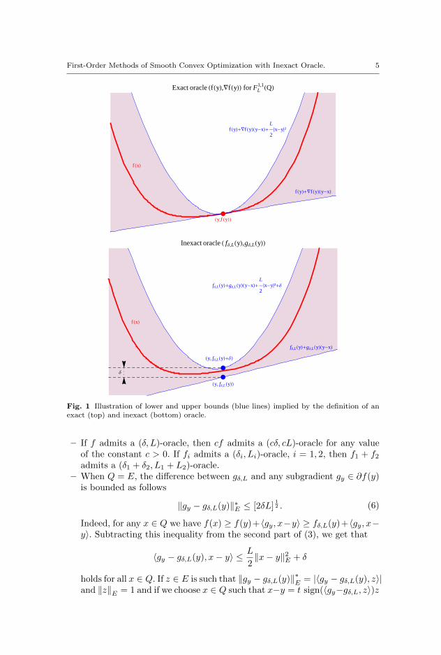
L (Q), the class of convex functions on convex set Q whose gra-dient is Lipschitz-continuous with constant L. It is well-known that functionsbelonging to this class satisfy

0 ≤ f(x)−(f(y) + 〈∇f(y), x− y〉

)≤ L

2‖x− y‖2E for all x, y ∈ Q, (2)

see the top of Figure 1. Moreover, it is easy to check that, for a given y,quantities f(y) and ∇f(y) are uniquely determined by this pair of inequalities.


Therefore, membership in F 1,1L (Q) can be characterized by the existence of an

oracle returning for each point y ∈ Q a pair (fL(y), gL(y)) ∈ R×E∗, necessarilyequal to (f(y),∇f(y)), satisfying

0 ≤ f(x)−(fL(y) + 〈gL(y), x− y〉

)≤ L

2‖x− y‖2E for all x ∈ Q

(both zeroth-order and first-order information are included in the oracle). Ourdefinition of an inexact oracle simply consists in introducing a given amountδ of tolerance in this pair of inequalities (see bottom of Figure 1).

Definition 1 Let function f be convex on convex set Q. We say that it isequipped with a first-order (δ, L)-oracle if for any y ∈ Q we can compute apair (fδ,L(y), gδ,L(y)) ∈ R× E∗ such that

0 ≤ f(x)−(fδ,L(y) + 〈gδ,L(y), x− y〉

)≤ L

2‖x− y‖2E + δ for all x ∈ Q. (3)

A function f belongs to F 1,1L (Q) if and only it admits a (0, L)-oracle, namely

(f0,L(y), g0,L(y)) = (f(y),∇f(y)). However, the class of functions admitting a(δ, L)-oracle is strictly larger, and includes non-smooth functions, as we willsee later.

2.2 Properties

We list here a few important properties of (δ, L)-oracles.

– A (δ, L)-oracle provides a lower δ-approximation of the function value.Indeed, taking x = y in (3), we obtain

fδ,L(y) ≤ f(y) ≤ fδ,L(y) + δ. (4)

– A (δ, L)-oracle provides a δ-subgradient of f at y ∈ Q, i.e.

gδ,L(y) ∈ ∂δf(y) = z ∈ E∗ : f(x) ≥ f(y) + 〈z, x− y〉 − δ ∀x ∈ Q.

Indeed, using the first inequality in (3) and (4), we have for all x, y ∈ Q

f(x) ≥ fδ,L(y) + 〈gδ,L(y), x− y〉 ≥ f(y) + 〈gδ,L(y), x− y〉 − δ. (5)

Methods of non-smooth convex optimization based on δ-subgradients havea long history (see e.g. [20,19,2,9] for subgradient methods, and [2,6,7] forproximal point and bundle methods). We will show later that a standardsubgradient can also satisfy the second inequality in (3), which opens thepossibility of using the concept of inexact oracle in the context of non-smooth convex optimization.

– A (δ, L) oracle can certify than an approximate solution has accuracy δ.Indeed, assuming gδ,L(y) satisfies 〈gδ,L(y), x−y〉 ≥ 0 for all x ∈ Q, we havethat fδ,L(y) ≤ f(x∗) = f∗ and therefore, using (4), we have f(y) ≤ f∗+ δ.


f HyL+Ñf HyLHy-xL+L

2Èx-yÈ²

f HxL

Hy,f HyLL

f HyL+Ñf HyLHy-xL

Exact oracle HfHyL,ÑfHyLL for FL1,1HQL

f∆,LHyL+g∆,LHyLHy-xL+

L

2Èx-yÈ²+∆

f HxL

Hy, f∆,LHyLL

Hy, f∆,LHyL+∆Lf∆,LHyL+g∆,LHyLHy-xL

∆

Inexact oracle H f∆,LHyL,g∆,LHyLL

Fig. 1 Illustration of lower and upper bounds (blue lines) implied by the definition of anexact (top) and inexact (bottom) oracle.

– If f admits a (δ, L)-oracle, then cf admits a (cδ, cL)-oracle for any valueof the constant c > 0. If fi admits a (δi, Li)-oracle, i = 1, 2, then f1 + f2

admits a (δ1 + δ2, L1 + L2)-oracle.– When Q = E, the difference between gδ,L and any subgradient gy ∈ ∂f(y)

is bounded as follows

‖gy − gδ,L(y)‖∗E ≤ [2δL]12 . (6)

Indeed, for any x ∈ Q we have f(x) ≥ f(y)+〈gy, x−y〉 ≥ fδ,L(y)+〈gy, x−y〉. Subtracting this inequality from the second part of (3), we get that

〈gy − gδ,L(y), x− y〉 ≤ L

2‖x− y‖2E + δ

holds for all x ∈ Q. If z ∈ E is such that ‖gy − gδ,L(y)‖∗E = |〈gy − gδ,L(y), z〉|and ‖z‖E = 1 and if we choose x ∈ Q such that x−y = t sign(〈gy−gδ,L, z〉)z


with t > 0, we obtain:

t‖gy − gδ,L(y)‖∗E ≤L

2t2 + δ ⇔ ‖gy − gδ,L(y)‖∗E ≤

L

2t+

δ

t. (7)

This upper bound attains its minimum [2δL]12 when t = [ 2δ

L ]12 . In particu-

lar, when Q = E, parameter t is free to take any real value, and we obtaininequality (6). For constrained problems, a similar bound can be obtainedin terms of the distance d(y, ∂Q) between y and the boundary of Q: letting

d(y, ∂Q) = maxr|‖x− y‖E ≤ r ⇒ x ∈ Q

we have that (7) holds for all t such that 0 < t ≤ d(y, ∂Q), so that

‖gy − gδ,L(y)‖∗E ≤

L2 d(y, ∂Q) + δ

d(y,∂Q) when 0 < d(y, ∂Q) ≤ [ 2δL ]

12 ,

[2δL]12 when d(y, ∂Q) ≥ [ 2δ

L ]12 .

– If E is endowed with the Euclidean norm ‖.‖2, the distance between exactand inexact gradient mappings can be bounded by the same quantities asthe distance between exact and inexact (sub)gradients. Recall that for anyγ > 0, g ∈ E∗ and y ∈ E, the gradient mapping Mγ(y, g), which replacesthe gradient for constrained problems, is defined by

Tγ(y, g) = arg minx∈Q〈g, x− y〉+

γ

2‖x− y‖2E (8)

Mγ(y, g) = γ(y − Tγ(y, g)). (9)

If f is subdifferentiable at point y, the exact gradient mapping for anysubgradient gy ∈ ∂f(y) is equal to Mγ(y, gy). Similarly, if an inexact (δ, L)oracle returns (fδ,L(y), gδ,L(y)) for point y, we call Mγ(y, gδ,L(y)) the in-exact gradient mapping. We are going to prove that the following holds

‖Mγ(y, gy)−Mγ(y, gδ,L(y))‖2 ≤ ‖gy − gδ,L(y)‖∗2 . (10)

First-order optimality conditions for (8) can be written as

〈g + γB(Tγ(y, g)− y), x− Tγ(y, g)〉 ≥ 0 ∀x ∈ Q. (11)

Applying those to Tγ(y, gy) and Tγ(y, gδ,L(y)) leads to

〈gy −BMγ(y, gy), x− Tγ(y, gy)〉 ≥ 0 ∀x ∈ Q〈gδ,L(y)−BMγ(y, gδ,L(y)), x− Tγ(y, gδ,L(y))〉 ≥ 0 ∀x ∈ Q

and specializing respectively to x = Tγ(y, gδ,L(y)) and x = Tγ(y, gy) gives

〈gy −BMγ(y, gy), Tγ(y, gδ,L(y))− Tγ(y, gy)〉 ≥ 0

〈gδ,L(y)−BMγ(y, gδ,L(y)), Tγ(y, gy)− Tγ(y, gδ,L(y))〉 ≥ 0 .

Using now (9) in the inner products, multiplying by γ and summing, weobtain

〈gy−BMγ(y, gy)−gδ,L(y)+BMγ(y, gδ,L(y)),Mγ(y, gy)−Mγ(y, gδ,L(y))〉 ≥ 0


and assuming that E is endowed with the Euclidean norm ‖.‖2 gives

〈gy−gδ,L(y),Mγ(y, gy)−Mγ(y, gδ,L(y))〉 ≥ ‖Mγ(y, gy)−Mγ(y, gδ,L(y))‖22 ,

from which the desired inequality (10) follows by Cauchy-Schwartz.

Characterizing the class of functions that can be endowed with a (δ, L)-oracle is an interesting open question. We provide below some necessary con-ditions in the simple case where Q = E and E is endowed with the Euclideannorm ‖.‖2. First of all, we establish the following inequality:

Theorem 1 If f is equipped with a (δ, L)-oracle, we have

1

2L(‖gδ,L(x)− gδ,L(y)‖∗2)2 ≤ f(y)− fδ,L(x)− 〈gδ,L(x), y − x〉+ δ ∀x, y ∈ E.

Proof Let x ∈ E and consider the function F (y) = f(y)− 〈gδ,L(x), y〉.As (fδ,L(y), gδ,L(y)) is a (δ, L)-oracle for f and (−〈gδ,L(x), y〉,−gδ,L(x)) is a(0, 0)-oracle for −〈gδ,L(x), y〉, the resulting sum of oracles (Fδ,L(y), Gδ,L(y)) =(fδ,L(y) − 〈gδ,L(x), y〉, gδ,L(y) − gδ,L(x)) is a (δ, L)-oracle for F (y). Using thelower bound in the definition of the oracle Fδ,L(x) + 〈Gδ,L(x), y − x〉 ≤ F (y),valid for any y, and the fact that Gδ,L(x) = 0, we derive

Fδ,L(x) ≤ F

(y − 1

LB−1Gδ,L(y)

)≤ Fδ,L(y) + 〈Gδ,L(y),− 1

LB−1Gδ,L(y)〉+

L

2

(∥∥∥∥ 1

LGδ,L(y)

∥∥∥∥∗2

)2

+ δ

= Fδ,L(y)− 1

2L

(‖Gδ,L(y)‖∗2

)2+ δ

which allows us to obtain

1

2L

(‖gδ,L(y)− gδ,L(x)‖∗2

)2 ≤ fδ,L(y)− fδ,L(x)− 〈gδ,L(x), y − x〉+ δ

≤ f(y)− fδ,L(x)− 〈gδ,L(x), y − x〉+ δ.

ut

As a Corollary, we have:

Corollary 1 If f is equipped with a (δ, L)-oracle, then we have for all x, y ∈ E

‖gδ,L(x)− gδ,L(y)‖∗2 ≤√L2 ‖x− y‖22 + 4Lδ

and for any gx ∈ ∂f(x) and any gy ∈ ∂f(y)

‖gx − gy‖∗2 ≤ (2√

2 + 2)√Lδ + L ‖x− y‖2 .


Proof Our first claim directly follows from

1

2L

(‖gδ,L(x)− gδ,L(y)‖∗2

)2 ≤ f(y)− fδ,L(x)− 〈gδ,L(x), y − x〉+ δ

(3)

≤ L

2‖x− y‖22 + 2δ.

Furthermore, for any gx ∈ ∂f(x) and gy ∈ ∂f(y), we have by (6):

‖gx − gδ,L(x)‖∗2 ≤√

2δL,

‖gy − gδ,L(y)‖∗2 ≤√

2δL,

and therefore (using the ‖ · ‖2 ≤ ‖ · ‖1 inequality for the last step)

‖gx − gy‖∗2 ≤ ‖gx − gδ,L(x)‖∗2 + ‖gδ,L(x)− gδ,L(x)‖∗2 + ‖gδ,L(y)− gy‖∗2

≤ 2√

2δL+

√L2 ‖x− y‖22 + 4Lδ

≤ (2√

2 + 2)√δL+ L ‖x− y‖2 .

ut

We conclude that the variation of subgradients of f is locally bounded, i.e.

‖gx − gy‖∗2 ≤ (2√

2 + 2)√Lδ + LR ∀x, y s.t. ‖x− y‖2 ≤ R.

Note however that this property is true for any subdifferentiable convex func-tion defined on the whole space E. Assume now that function f is endowedwith a family of (δ, L(δ))-oracles and consider the following situations:

–

limδ→0

L(δ) = L < +∞

In this case we have ‖gx − gy‖∗2 ≤ L ‖x− y‖2 and f must be a smoothconvex function with a Lipschitz-continuous gradient.

–

limδ→∞

L(δ) = 0 and limδ→∞

L(δ)δ = C < +∞,

which is the case for example when L(δ) = Cδ . We have ‖gx − gy‖∗2 ≤

(2√

2 + 2)√C so that f must be a convex function with bounded variation

of subgradients.–

limδ→∞

L(δ) = 0 and limδ→∞

L(δ)δ = 0

which would happen for example when L(δ) = Cδ2 . We have in that case

that ‖gx − gy‖∗2 ≤ 0 and f must be a constant function.


2.3 Examples

To conlude this section, we consider four simple examples of inexact oracle.More sophisticated examples will be given in Section 3.

a. Computations at shifted points. Let function f ∈ F 1,1M (Q) be endowed with

an oracle providing at each point y ∈ Q the exact values of function andgradient, albeit computed at a shifted point y different from y. Let us showthat such an oracle can be converted into a (δ, L)-oracle with

δ = M ‖y − y‖2E , L = 2M.

Convexity of f implies the following inequality for any x ∈ Q

f(x) ≥ f(y) + 〈∇f(y), x− y〉

= f(y) + 〈∇f(y), y − y〉+ 〈∇f(y), x− y〉.

Therefore, to satisfy the first inequality in (3) we can choose fδ,L(y)def= f(y)+

〈∇f(y), y − y〉, and gδ,L(y)def= ∇f(y). In order to prove the second inequality

in (3), note that we have for all x ∈ Q

f(x)(2)

≤ f(y) + 〈∇f(y), x− y〉+ M2 ‖x− y‖

2E

= f(y) + 〈∇f(y), y − y〉+ 〈∇f(y), x− y〉+ M2 ‖x− y‖

2E .

Since ‖ · ‖2E is a convex function, we have

‖x− y‖2E =

∥∥∥∥1

2

(2(x− y)

)+

1

2

(2(y − y)

)∥∥∥∥2

E

(12)

≤ 1

2‖2(x− y)‖2E +

1

2‖2(y − y)‖2E = 2‖y − y‖2E + 2‖x− y‖2E .(13)

Therefore,

f(x) ≤ fδ,L(y) + 〈gδ,L(y), x− y〉+M ‖x− y‖2E +M ‖y − y‖2E .

We can therefore choose L = 2M and δ = M‖y − y‖2E to satisfy the (δ, L)-oracle definition.


b. Convex problems with weaker level of smoothness. Let us show that thenotion of (δ, L)-oracle can be useful for solving the problems with exact first-order information but with a lower level of smoothness. Let function f beconvex and subdifferentiable on Q. For each y ∈ Q, denote by g(y) an arbitraryelement of the subdifferential ∂f(y). Assume that f satisfies the followingHolder condition:

‖g(x)− g(y)‖∗E ≤ Lν ‖x− y‖νE , ∀x, y ∈ Q, (14)

where ν ∈ [0, 1], and Lν < +∞. This condition leads to the following inequal-ity:

f(x) ≤ f(y) + 〈g(y), x− y〉+ Lν1+ν ‖x− y‖

1+νE , ∀x, y ∈ Q. (15)

Denote the class of such functions by F 1,νLν

(Q). When ν = 1, we get func-tions with Lipschitz-continuous gradient. For ν < 1, we get a lower level ofsmoothness. In particular, when ν = 0, we obtain functions whose subgradi-ents have bounded variation. Clearly, the latter class includes functions whosesubgradients are uniformly bounded by M (just take L0 = 2M).

Let us fix ν ∈ [0, 1) and an arbitrary δ > 0 . We are going to find a constantA(δ, ν) such that for any function f ∈ F 1,ν

Lν(Q) we have

f(x)− f(y)− 〈g(y), x− y〉 ≤ A(δ,ν)2 ‖x− y‖2E + δ, ∀x, y ∈ Q. (16)

Comparing (15) and (16), we need choose A(δ, ν) such that

Lν1 + ν

‖x− y‖1+νE ≤ A(δ, ν)

2‖x− y‖2E + δ .

Since t = ‖x− y‖2E can take any nonnegative value, we may choose

A(δ, ν) = 2 maxt≥0

Lν

1+ν t−1+ν − δt−2

= Lν

[Lν2δ ·

1−ν1+ν

] 1−ν1+ν

.

(the latter expression is obtained after straightforward computations, the op-

timal value of t in the maximization being t∗ =[Lν2δ ·

1−ν1+ν

]− 11+ν

). This means

that the exact first-order information (f(y), g(y)) also constitutes an inexact(δ, A(δ, ν))-oracle. We will therefore be able to apply the methods from Sec-tions 4 and 5, initially devoted for smooth problems, to the minimization ofthe non- or weakly smooth objective f .

For example, for functions with bounded variation of subgradients (ν = 0)we have

A(δ, 0) =L2

0

2δ . (17)

so that a (δ,L2

0

2δ )-oracle is available for all values of δ > 0.Note that parameter δ does not represent an actual accuracy: it can be

chosen arbitrarily, independently of the answer of the oracle. In particular, δcan be chosen as small as we want, at the price of a larger value for Lipschitz

constant L of the (δ, L)-oracle, which grows as O(δ−

1−ν1+ν

). Section 8 will

describe the details and consequences of the application of first-order methodof smooth convex optimization to non-smooth or weakly smooth functions.


Remark 1 This analysis can easily be extended to the case where δ-subgradientswith bounded variations are used instead of exact subgradients. We obtain inthis case a (2δ, A(δ, ν))-oracle.

c. Function smoothed by local averaging. Another typical approach in orderto apply first-order method of F 1,1

L (E) to a non-smooth function consists insmoothing the function by averaging of first-order information. Assume thatE is endowed with an Euclidean norm and consider a non-smooth convexfunction f ∈ F 1,0

M (E). Let r > 0, y ∈ E, and define

fδ(y) =1

Vr

∫‖z−y‖2≤r

f(z) dz

∇fr(y) = gr(y) =1

Vr

∫‖z−y‖2≤r

g(z) dz

where Vr denotes the volume of a Euclidean ball with radius r, and g(z) :‖z − y‖2 ≤ r is a measurable selection of subgradients of f in this ball. As fis convex and Lipschitz-continuous with constant M we have

0 ≤ f(x)− f(z)− 〈g(z), x− z〉 ≤M ‖x− z‖2 ∀x, z ∈ E

and therefore

f(x) ≥ f(z) + 〈g(z), x− y〉+ 〈g(z), y − z〉 ∀x, y, z ∈ Ef(x) ≤ f(z) + 〈g(z), x− y〉+ 〈g(z), y − z〉+M ‖x− z‖2 ∀x, y, z ∈ E.

Averaging now these two inequalities with respect to z over the ball z :‖z − y‖2 ≤ r, we obtain for all x, y ∈ Z

f(x) ≥ fr(y) + 〈gr(y), x− y〉 −Mr

f(x) ≤ fr(y) + 〈gr(y), x− y〉+Mr +M

Vr

∫‖z−y‖2≤r

‖x− z‖2 dz

(where we used that |〈g(z), y − z〉| ≤ ‖g(z)‖∗2‖y − z‖2 ≤ Mr). Furthermore,we have

‖x− z‖2(13)

≤√

2 ‖x− y‖22 + 2 ‖z − y‖22 ≤2 ‖x− y‖22 + 2 ‖z − y‖22

2r+r

2

(where the second inequality comes from the arithmetic-geometric inequality),and therefore

f(x) ≤ fr(y) + 〈gr(y), x− y〉+3

2Mr +M

‖x− y‖22r

+M

Vr

∫‖z−y‖2≤r

‖z − y‖2 dz

≤ fr(y) + 〈gr(y), x− y〉+5

2Mr +M

‖x− y‖22r

.

Finally, choosing fδ,L(y) = fr(y)−Mr, gδ,L(y) = gr(y), δ = 7Mr2 and L = 2M

r ,

we obtain a (δ, L) = (7Mr2 , 2M

r ) = (δ, 7M2

δ )-oracle. Note that the dependenceof L in M and δ is similar to that of the previous example, where subgradientsare used directly instead of being averaged.


d. Functions approximated by a smooth function When a function f can bewell approximated by a smooth convex function f , in the sense that theirdifference is bounded, the exact values of f and its gradient provide an inexactoracle for f . Indeed, assume that there exists a smooth convex function f ∈F 1,1L (Q) such that f is a δ-lower approximation of f on all Q, i.e.

0 ≤ f(y)− f(y) ≤ δ ∀y ∈ Q.

We can then show that

f(x) ≥ f(x) ≥ f(y) + 〈∇f(y), x− y〉 ∀x, y ∈ Q,

(using convexity of f), and

f(x) ≤ f(x) + δ ≤ f(y) + 〈∇f(y), x− y〉+L

2‖x− y‖2E + δ ∀x, y ∈ Q.

(using Lipschitz continuity of f), which shows that (f(y),∇f(y)) is a (δ, L)-oracle for f .

One might wonder whether all inexact oracles can be obtained in thatfashion, i.e. whether any inexact oracle can be seen as an exact oracle fora smooth approximation f . It turns out that is not the case: indeed, as wehave seen earlier, when f has subgradients with bounded variation, its exactfunction values and subgradients can be seen as a (δ, L)-oracle (for arbitraryvalue of δ). Clearly, such an oracle cannot be at the same time equal to theexact function values and gradient of any smooth function f .

Finally, note that the above result can be readily extended to the casewhen the δ-lower approximation f is not necessarily smooth but is equippedwith an inexact (δ′, L) oracle: we can then show that the inexact oracle of falso constitutes an inexact (δ + δ′, L) oracle for f .

3 Inexact oracle for functions defined by an optimization problem

3.1 Accuracy measures for approximate solutions

In this section, we consider smooth convex optimization problems of the form (1)whose objective function is defined by another optimization problem:

f(x) = maxu∈U

Ψ(x, u), (18)

where U is a convex set of a finite dimensional space F endowed with the norm‖.‖F and for any x ∈ Q function Ψ(x, ·) is smooth and (strongly) concave withconcavity parameter κ ≥ 0 . Computation of f and its gradient requires theexact solution of this auxiliary problem. However, in practice, such a solutionmight often be impossible or too costly to compute, so that an approximatesolution has to be used instead.


We will measure the accuracy of an approximate solution ux for problem(18) in three different ways:

V1(ux) = maxu∈U〈∇2Ψ(x, ux), u− ux〉,

V2(ux) = maxu∈U

[Ψ(x, u)− Ψ(x, ux) + κ

2 ‖ux − u‖2F

],

V3(ux) = maxu∈U

[Ψ(x, u)− Ψ(x, ux)] .

(19)

Since Ψ(x, ·) is strongly concave, we have:

Ψ(x, u) ≤ Ψ(x, ux) + 〈∇2Ψ(x, ux), u− ux〉 − κ2 ‖u− ux‖

2F , ∀u ∈ U.

Therefore our three measures are related by

V3(ux) ≤ V2(ux) ≤ V1(ux).

For a given level of accuracy δ > 0, the condition V1(ux) ≤ δ is the strongest,and condition V3(ux) ≤ δ is the most relaxed.

We describe below three classes of max-type functions for which the ap-proximate solution of subproblem (18), when satisfying one of the conditionsVi(ux) ≤ δ, allows the construction of a (δ, L)-oracle.

Let us show first how to satisfy stopping criteria (19) in practice. Themost common criterion is the third one. It amounts to estimating the optimal-ity gap in the value of objective function. Many optimization methods offerdirect control of this criterion. Other criteria might be more difficult to han-dle. Therefore, let us describe a “brute force” approach designed to satisfy thestrongest V1 criterion (Here we assume that F is endowed with an Euclideannorm).

Let Du <∞ be the diameter of U . Let us choose u0 ∈ U and form a newfunction

Ψ(x, u) = Ψ(x, u)− 12µ‖u− u0‖22.

Denote by Vi(u) the corresponding accuracy measures, and u∗x = arg maxu∈U

Ψ(x, u).

For any u ∈ U we obtain

0 ≥ 〈∇2Ψ(x, u∗x), u− u∗x〉 = 〈∇2Ψ(x, u∗x), ux − u∗x〉+ 〈∇2Ψ(x, u∗x), u− ux〉

≥ −V3(ux) + 〈∇2Ψ(x, u∗x)−∇2Ψ(x, ux), u− ux〉+ 〈∇2Ψ(x, ux), u− ux〉

≥ −V3(ux)− ‖∇2Ψ(x, u∗x)−∇2Ψ(x, ux)‖∗2Du + 〈∇2Ψ(x, ux), u− ux〉.

Since ∇2Ψ(x, ·) is Lipschitz continuous on U with constant L, we get

1

2L

(∥∥∇2Ψ(x, u∗x)−∇2Ψ(x, ux)∥∥∗

2

)2

≤ Ψ(x, u∗x)− Ψ(x, ux) + 〈∇2Ψ(x, u∗x), ux − u∗x〉

≤ Ψ(x, u∗x)− Ψ(x, ux) = V3(ux).


and therefore:

V1(ux) ≤ V1(ux) + µD2u

(2)

≤ V3(ux) +Du[2LV3(ux)]1/2 + µD2u.

Thus, if we choose µ = δ3D2

u, we can get the desired level of V1(ux) by ensuring

V3(ux) ≤ δ2

18LD2u

. Note that function Ψ(x, ·) is strongly concave. Therefore, the

complexity of its maximization in the scale V3 depends logarithmically on thedesired accuracy. If this is done, for example, by a FGM, it requires at most

O(L1/2

δ1/2ln 1

δ ) iterations (see section 2.2 in [14]).

3.2 Functions obtained by smoothing techniques

Let U be a closed, convex set of a finite dimensional space F endowed withthe norm ‖·‖F , and

Ψ(x, u) = G(u) + 〈Au, x〉,where A : F → E∗ is a linear operator, and G(u) is a differentiable, stronglyconcave function with concavity parameter κ > 0. Under these assumptions,optimization problem (18) has only one optimal solution u∗x. Moreover, f isconvex and smooth with Lipschitz-continuous gradient ∇f(x) = Au∗x. Thecorresponding Lipschitz-constant is equal to

L(f) = 1κ‖A‖

2F→E∗ (20)

where ‖A‖F→E∗ = max‖Au‖E∗ : ‖u‖F = 1. The importance of this classof functions is justified by the smoothing approach for non-smooth convexoptimization (see [15,16,17,4]).

Suppose that for all y ∈ Q we can find a point uy ∈ U satisfying condition

V3(uy) = Ψ(y, u∗y)− Ψ(y, uy) ≤ δ2 . (21)

Let us show that this allows us to construct an (δ, 2L(f))-oracle. Indeed, sinceΨ(·, u) is convex, for all u ∈ U , we have

f(x) = Ψ(x, u∗x) ≥ Ψ(x, uy) ≥ Ψ(y, uy) + 〈∇1Ψ(y, uy), x− y〉

= fδ,L(y) + 〈gδ,L(y), x− y〉,(22)

where fδ,L(y)def= Ψ(y, uy), gδ,L(y)

def= ∇1Ψ(y, uy) = Auy, and L will be speci-

fied later. Further, note that

〈∇1Ψ(y, u∗y), x− y〉 = 〈gδ,L(y), x− y〉+ 〈A(u∗y − uy), x− y〉. (23)

Since f has Lipschitz-continuous gradient, we have:

f(x) ≤ f(y) + 〈∇f(y), x− y〉+ L(f)2 ‖x− y‖2E

= f(y) + 〈∇Ψ1(y, u∗y), x− y〉+ L(f)2 ‖x− y‖2E

(23)= f(y) + 〈gδ,L(y), x− y〉+ L(f)

2 ‖x− y‖2E + 〈A(u∗y − uy), x− y〉.


On the other hand, we have:

〈A(u∗y − uy), x− y〉 ≤∥∥u∗y − uy∥∥F ∥∥AT (x− y)

∥∥∗E

(20)

≤ κ2

∥∥u∗y − uy∥∥2

F+ L(f)

2 ‖x− y‖2E .

Therefore,

f(x) ≤ f(y) + 〈gδ,L(y), x− y〉+ L(f) ‖x− y‖2E + κ2

∥∥u∗y − uy∥∥2

F.

Since Ψ is strongly concave, κ2

∥∥uy − u∗y∥∥2

F≤ Ψ(y, u∗y)− Ψ(y, uy). Thus,

f(x) ≤ Ψ(y, uy) + 2(Ψ(y, u∗y)− Ψ(y, uy)) + 〈gδ,L(y), x− y〉+ L(f) ‖x− y‖2E .

In view of conditions (21) and (22), we have proved that the pair (Ψ(y, uy), Auy),satisfying condition (21), corresponds to an (δ, L)-oracle with L = 2L(f).

3.3 Moreau-Yosida regularization

In this section, we consider functions of the form

f(x) = minu∈U

L(x, u)

def= h(u) + κ

2 ‖u− x‖22

, (24)

where h is a smooth convex function on a convex set U ⊂ Rn endowed with theusual Euclidean norm ‖x‖22 = 〈x, x〉. The function f is convex with Lipschitz-continuous gradient ∇f(x) = κ(x− u∗x), where u∗x denotes the unique optimalsolution of the problem (24). The Lipschitz constant of the gradient is equalto κ.

Instead of solving exactly the problem (24), we compute a feasible solutionux satisfying

V2(ux) = maxu∈U

L(x, ux)− L(x, u) + κ

2 ‖u− ux‖22

≤ δ. (25)

(Since L is convex in u, we inverted the sign in the definition of V2 in (19).)Let us show that for all x ∈ Q the objects

fδ,L(x) = L(x, ux)− δ = h(ux) + κ2 ‖ux − x‖

22 − δ,

gδ,L(x) = ∇1L(x, ux) = κ(x− ux)(26)


correspond to an answer of an (δ, L)-oracle with L = κ. Indeed,

f(x) = L(x, u∗x) ≥ L(y, u∗x) + κ2 〈y − x, 2u

∗x − x− y〉

(25)

≥ L(y, uy) + κ2 ‖u

∗x − uy‖22 − δ + κ

2 〈y − x, 2u∗x − x− y〉

= L(y, uy) + κ〈y − uy, x− y〉+ κ2 ‖u

∗x − uy‖

22 − δ

+κ2 〈y − x, 2u

∗x − 2uy + y − x〉

= L(y, uy) + κ〈y − uy, x− y〉 − δ

+κ2

(‖u∗x − uy‖

22 + ‖y − x‖22 + 2〈y − x, u∗x − uy〉

)≥ L(y, uy) + κ〈y − uy, x− y〉 − δ.

Thus, we satisfy the first inequality in (3) with the values defined by (26).Further, for all x, y ∈ Q we have

f(x) = h(u∗x) + κ2 ‖u

∗x − x‖

22 ≤ h(uy) + κ

2 ‖uy − x‖22

= h(uy) + κ2 ‖uy − y‖

22 + κ

2 〈x− y, x+ y − 2uy〉

= L(y, uy) + κ〈y − uy, x− y〉+ κ2 ‖y − x‖

22 .

Thus, in view of definition (26), we have proved the second inequality in (3)with L = κ.

3.4 Functions defined by Augmented Lagrangians

Consider the following convex problem:

maxu∈Uh(u) : Au = 0 , (27)

where h is a smooth concave function on the convex set U ⊂ F , F is a finite-dimensional space, and A : F → E∗ is a linear operator. Let E be endowedwith the Euclidean norm ‖.‖2. In the Augmented Lagrangian approach, weneed to solve the dual problem

minx∈E

f(x), (28)

where

f(x)def= max

u∈U

[Ψ(x, u)

def= h(u) + 〈Au, x〉 − κ

2 (‖Au‖∗2)2]. (29)

It is well-known that f is a convex smooth function with Lipschitz-continuousgradient

∇f(x) = Au∗x,


where u∗x denotes any optimal solution of the optimization problem (29). TheLipschitz constant of the gradient is equal to 1

κ .Assume that, instead of solving (28) exactly, we compute an approximate

solution ux ∈ U such that

V1(ux) = maxu∈U

〈∇2Ψ(x, ux), u− ux〉

= maxu∈U

〈∇h(ux) +ATx− κATB−1Aux, u− ux〉 ≤ δ.(30)

Let us show that the objects

fδ,L(x) = Ψ(x, ux), gδ,L(x) = ∇1Ψ(x, ux) = Aux (31)

correspond to a (δ, L)-oracle with L = 1κ . Indeed, for all x, y ∈ E we have

f(x) = maxu∈U

h(u) + 〈Au, x〉 − κ

2 (‖Au‖∗2)2

≥ h(uy) + 〈Auy, x〉 − κ2 (‖Auy‖∗2)2 = Ψ(y, uy) + 〈Auy, x− y〉.

Thus, in view of definition (31), the first inequality in (3) is proved. Further,

f(x) ≤ maxu∈Uh(uy) + 〈∇h(uy), u− uy〉+ 〈Au, x〉 − κ

2 (‖Au‖∗2)2

(30)

≤ maxu∈Uh(uy)− 〈AT y − κATB−1Auy, u− uy〉+ 〈Au, x〉 − κ

2 (‖Au‖∗2)2+ δ

= Ψ(y, uy) + 〈Auy, x− y〉

+ maxu∈U

〈A(u− uy), x− y〉 − κ

2 (‖A(u− uy)‖∗2)2

+ δ.

Thus, in view of (31), we have proved the second inequality in (3) with L = 1κ .

4 Gradient methods with inexact oracle

Consider the problem (1), where f is endowed with an inexact (δ, L)-oracle.In this section, we will use the Euclidean norm ‖.‖2. As usual when dealingwith constrained problems, we assume that the gradient mapping TL(x, g) iscomputable for any x ∈ Q and g ∈ E∗, see (8).

4.1 Primal gradient method

The classical (primal) gradient method can be adapted in a straightforwardmanner to accept first-order information from an inexact oracle: it is enoughto replace the true gradient by its approximate counterpart gδ,L. Moreover,


we allow the parameters (δk, Lk) of the inexact oracle to be different for eachiteration k. We obtain

Initialization: Choose x0 ∈ Q.

Iteration (k ≥ 0): 1. Choose δk and Lk.

2. Compute (fδk,Lk(xk), gδk,Lk(xk)).

3. Compute xk+1 = TLk(xk, gδk,Lk(xk)).

(PGM)

Theorem 2 For k ≥ 1, we have

k−1∑i=0

1Li

[f(xi+1)− f(x∗)] ≤ 12‖x0 − x∗‖22 +

k−1∑i=0

δiLi. (32)

Proof Denote rk = ‖xk − x∗‖22, fk = fδk,Lk(xk), and gk = gδk,Lk(xk). Then

r2k+1 = r2

k + 2〈B(xk+1 − xk), xk+1 − x∗〉 − ‖xk+1 − xk‖22

(11)

≤ r2k + 2

Lk〈gk, x∗ − xk+1〉 − ‖xk+1 − xk‖22

= r2k + 2

Lk〈gk, x∗ − xk〉 − 2

Lk[〈gk, xk+1 − xk〉+ Lk

2 ‖xk+1 − xk‖22]

(3)

≤ r2k + 2

Lk[f(x∗)− fk]− 2

Lk[f(xk+1)− fk − δk].

Summing up these inequalities for i = 0, . . . , k − 1, we obtain (32). utWhen exact first-order information is used (δi = 0, Li = L), it is well-

known that sequence f(xi) must be decreasing. This is no longer true whenan inexact oracle is used. Therefore, let us define

xk =∑k−1i=0 L

−1i xi+1∑k−1

i=0 L−1i

∈ Q.

Since f is convex, we have

f(xk)− f(x∗) ≤12‖x0−x∗‖22 +

∑k−1i=0 L

−1i δi∑k−1

i=0 L−1i

. (33)

In the case when the oracle accuracy is constant (δi = δ, Li = L), we have

f(xk)− f(x∗) ≤ LR2

2k + δ, Rdef= ‖x0 − x∗‖2 . (34)

Thus, there is no error accumulation, and the upper bound for the objectivefunction accuracy decreases with k and asymptotically tends to δ. Hence, if

an accuracy ε on the objective function is required (with ε > δ), k = LR2

2(ε−δ)iterations are sufficient. In particular, we see that PGM allows the oracleaccuracy to be of the same order as the desired accuracy for the objectivefunction.


4.2 Dual gradient method

This method [18] generates two sequences xkk≥0 and ykk≥0.

Initialization: Choose x0 ∈ Q.

Iteration (k ≥ 0): 1. Choose δk and Lk.

2. Compute (fδk,Lk(xk), gδk,Lk(xk)).

3. Compute xk+1 = arg minx∈Q

[k∑i=0

1Li〈gδi,Li(xi), x− xi〉+ 1

2‖x− x0‖22].

(35)

Define yk = TLk(xk, gδk,Lk(xk)), k ≥ 0.

Theorem 3 For any k ≥ 0 we have

k∑i=0

1Li

[f(yi)− f(x∗)] ≤ 12‖x0 − x∗‖22 +

k∑i=0

δiLi. (36)

Proof For k ≥ 0, denote fk = fδk,Lk(xk), gk = gδk,Lk(xk), and

ψk(x) =k∑i=0

1Li

[fi + 〈gi, x− xi〉] + 12‖x− x0‖22, ψ∗k = min

x∈Qψk(x).

In view of the first inequality in (3), we have for all x ∈ Q

ψ∗k ≤ ψk(x) ≤∑ki=0

1Lif(x) + 1

2 ‖x− x0‖22 . (37)

Let us prove that ψ∗k ≥k∑i=0

1Li

[f(yi) − δi]. Indeed, this inequality is valid for

k = 0:

f(y0)(3)

≤ f0 + 〈g0, y0 − x0〉+ L0

2 ‖y0 − x0‖22 + δ0 = L0ψ∗0 + δ0.

Assume it is valid for some k ≥ 1. Since Ψk(x) is strongly convex, we have:

ψk(x) ≥ ψ∗k + 12‖x− xk+1‖22, x ∈ Q

Therefore,

ψ∗k+1 = minx∈Q

ψk(x) + 1

Lk+1[fk+1 + 〈gk+1, x− xk+1〉]

≥ ψ∗k + 1

Lk+1minx∈Q

fk+1 + 〈gk+1, x− xk+1〉+ Lk+1

2 ‖x− xk+1‖22

(3)

≥ ψ∗k + 1Lk+1

(f(yk+1)− δk+1).


Hence, using our inductive assumption, we can prove that ψ∗k ≥k∑i=0

1Li

[f(yi)−

δi] for all k ≥ 0. To conclude we combine this fact with inequality (37) forx = x∗. ut

As for the Primal Gradient Method, we define

yk =∑ki=0 L

−1i yi∑k

i=0 L−1i

∈ Q,

and obtain the same upper bound

f(yk)− f(x∗) ≤12‖x0−x∗‖22 +

∑ki=0 L

−1i δi∑k

i=0 L−1i

, k ≥ 0. (38)

Since we obtain the same convergence results for both primal and dual gradientmethods, we will refer to both as Classical Gradient Methods (CGM) in therest of this paper.

5 Fast gradient method with inexact oracle

5.1 Convergence analysis

In this section, we adapt one of the last versions of Fast Gradient Method(FGM) developed in [15]. Let d(x) be a prox-function, differentiable and stronglyconvex on Q, and let x0 = arg min

x∈Qd(x) be its prox-center.

Translating and scaling d if necessary, we can always ensure that

d(x0) = 0, d(x) ≥ 12 ‖x− x0‖2E , ∀x ∈ Q. (39)

(here ‖·‖E denotes any norm on E). Let αk∞k=0 be a sequence of reals suchthat

α0 ∈ (0, 1],α2k

Lk≤ Ak

def=

k∑i=0

αiLi, k ≥ 0. (40)

Define τk = αk+1

Ak+1Lk+1, k ≥ 0 and consider the following method.

Initialization: Choose δ0, L0, and x0 = arg minx∈Q

d(x).

Iteration (k ≥ 0): 1. Compute (fδk,Lk(xk), gδk,Lk(xk)).

2. Compute yk = TLk(xk, gδk,Lk(xk)).

3. Compute zk = arg minx∈Qd(x) +

k∑i=0

αiLi〈gδi,Li(xi), x− xi〉.

4. Choose δk+1 and Lk+1. Define xk+1 = τkzk + (1− τk)yk.

(FGM)

Denote ψ∗k = minx∈Qd(x) +

∑ki=0

αiLi

[fδi,Li(xi) + 〈gδi,Li(xi), x− xi〉].


Theorem 4 For all k ≥ 0, we have Akf(yk) ≤ ψ∗k + Ek with Ek =k∑i=0

Aiδi.

Proof Denote fk = fδk,Lk(xk), and gk = gδk,Lk(xk). For k = 0, we have

ψ∗0 = minx∈Q

d(x) + α0

L0[f0 + 〈g0, x− x0〉]

(39)

≥ α0

L0minx∈Q

f0 + 〈g0, x− x0〉+ L0

2 ‖x− x0‖2E (3)

≥ α0

L0[f(y0)− δ0].

Assume now that the statement of the theorem is true for some k ≥ 0.Optimality conditions for the optimization problem solved at Step 3 imply

〈∇d(zk) +∑ki=0

αiLigi, x− zk〉 ≥ 0, ∀x ∈ Q.

Hence, in view of strong convexity of d,

d(x) ≥ d(zk) + 〈∇d(zk), x− zk〉+ 12‖x− zk‖

2E

≥ d(zk) +∑ki=0

αiLi〈gi, zk − x〉+ 1

2 ‖x− zk‖2E .

Thus, we have for all x ∈ Q that

d(x) +k+1∑i=0

αiLi

[fi + 〈gi, x− xi〉] ≥ d(zk) +k∑i=0

αiLi

[fi + 〈gi, zk − xi〉]

+ 12 ‖x− zk‖

2E + αk+1

Lk+1[fk+1 + 〈gk+1, x− xk+1〉].

We have obtained

ψ∗k+1 ≥ ψ∗k + minx∈Q 1

2 ‖x− zk‖2E + αk+1

Lk+1[fk+1 + 〈gk+1, x− xk+1〉].

On the other hand, we have

ψ∗k + αk+1

Lk+1[fk+1 + 〈gk+1, x− xk+1〉]

≥ Akf(yk)− Ek + αk+1

Lk+1[fk+1 + 〈gk+1, x− xk+1〉]

(3)

≥ Ak[fk+1 + 〈gk+1, yk − xk+1〉]− Ek + αk+1

Lk+1[fk+1 + 〈gk+1, x− xk+1〉]

= Ak+1fk+1 + 〈gk+1, Ak(yk − xk+1) + αk+1

Lk+1(x− xk+1)〉 − Ek.

Taking into account that

Ak(yk − xk+1) + αk+1

Lk+1(x− xk+1)

= Akτk(yk − zk) + αk+1

Lk+1x− αk+1

Lk+1τkzk − αk+1

Lk+1(1− τk)yk = αk+1

Lk+1(x− zk),


we obtain

ψ∗k + αk+1

Lk+1[fk+1 + 〈gk+1), x− xk+1〉] ≥ Ak+1fk+1 + αk+1

Lk+1〈gk+1, x− zk〉 − Ek.

Therefore,

ψ∗k+1 ≥ Ak+1fk+1 − Ek + minx∈Q 1

2 ‖x− zk‖2E + αk+1

Lk+1〈gk+1, x− zk〉

= Ak+1

[fk+1 + min

x∈Q 1

2Ak+1‖x− zk‖2E + τk〈gk+1, x− zk〉

]− Ek

(40)

≥ Ak+1

[fk+1 + minx∈Q τ

2kLk+1

2 ‖x− zk‖2E + τk〈gk+1, x− zk〉]− Ek.

For x ∈ Q, define y = τkx+ (1− τk)yk. Since y−xk+1 = τk(x− zk), we obtain

minx∈Q

τ2kLk+1

2 ‖x− zk‖2E + τk〈gk+1, x− zk〉

= miny

Lk+1

2 ‖y − xk+1‖2E + 〈gk+1, y − xk+1〉 : y ∈ τkQ+ (1− τk)yk

≥ min

y∈Q

Lk+1

2 ‖y − xk+1‖2E + 〈gk+1, y − xk+1〉.

(41)

Therefore,we have:

Ψ∗k+1 ≥ Ak+1

[fk+1 + min

x∈Q τ

2kLk+1

2 ‖x− zk‖2E + τk〈gk+1, x− zk〉]− Ek

(3),(41)

≥ Ak+1f(yk+1)− Ek −Ak+1δk+1,

and we get Ak+1f(yk+1) ≤ Ψk+1 + Ek+1 with Ek+1 = Ek +Ak+1δk+1. ut

Theorem 5 For all k ≥ 0, we have f(yk)− f∗ ≤ 1Ak

(d(x∗) +

∑ki=0Aiδi

).

Proof Denote fi = fδi,Li(xi), and gi = gδi,Li(xi). Then

ψ∗k = minx∈Q

d(x) +

k∑i=0

αiLi

[fi + 〈gi, x− xi〉]

≤ d(x∗) +k∑i=0

αiLi

[fi + 〈gi, x∗ − xi〉] ≤ d(x∗) +Akf(x∗).

The proof now simply follows from the recurrence established in Theorem 4.ut


A simple choice for the sequence αi consists in letting αi = i+12 . In that

case, the sequence of Lipschitz constants must satisfy the inequality (k+1)2

4Lk

(40)

≤k∑i=0

i+12Li

, i.e.

Lk ≥ (k+1)2

2 /

[k∑i=0

i+1Li

].

(It is true, for example, for any increasing sequence Lkk≥0.) In this case, weobtain

f(yk)− f∗ ≤ 1∑ki=0

i+12Li

(d(x∗) +

k∑i=0

i∑j=0

j+12Lj

δi

).

If the parameters of the inexact oracle are constant (δi = δ, Li = L), we

have Ak = (k+1)(k+2)4L , τk = 2

k+3 , and therefore

f(yk)− f∗ ≤ 4Ld(x∗)(k+1)2 + 1

(k+1)(k+2)

k∑i=0

(i+ 1)(i+ 2)δ.

Since∑ki=0(i+ 1)(i+ 2) = 1

6 (k + 1)(k + 2)(2k + 6), we obtain

f(yk)− f∗ ≤ 4Ld(x∗)(k+1)(k+2) + 1

6 (2k + 6)δ = 4LR2

(k+1)2 + 13 (k + 3)δ (42)

where Rdef=√d(x∗).

5.2 Error accumulation

Contrarily to the classical gradient methods, the use of inexact oracle in FGMresults in error accumulation. Indeed, while the first term in (42) decreasesas O( 1

k2 ), the second term is increasing in k, and this FGM used with aninexact oracle is asymptotically divergent. Section 8.3 will prove that erroraccumulation and divergence are unavoidable for all fast first-order methods.

We now study the non-asymptotic behavior of FGM, and consider twocases.

a. Oracle accuracy δ is fixed. In this case, we can find the number of iterationsk∗ that achieves the minimal guaranteed residual for the objective function.We let

E(k) = 4Ld(x∗)(k+1)2 + 1

3 (k + 1)δ + 23δ.

This function is convex in k and its minimum is reached at iteration k∗

k∗ = 2 3

√3Ld(x∗)

δ − 1

for which the guaranteed accuracy for the objective function is

E(k∗) = Θ(δ2/3L1/3R2/3).


b. Oracle accuracy δ can be chosen. Let us assume that parameter L of theinexact oracle is independent on δ. If we need to reach accuracy ε for theresidual f(yk)− f∗, it is enough to perform k iterations, with k satisfying twoinequalities:

4Ld(x∗)(k+1)2 ≤

ε2 ,

13 (k + 3)δ ≤ ε

2 .

The first inequality gives us k ≥√

8Ld(x∗)ε − 1, and the second one gives

k ≤ 3ε2δ − 3. Therefore attaining both ε

2 accuracies is possible if and only if

δ ≤ 3ε3/2

2√

8Ld(x∗)+4√ε. (43)

In conclusion, if we choose the oracle accuracy satisfying relation (43), thenafter

k(ε) =√

8Ld(x∗)ε − 1

iterations, we obtain a point yk(ε) ∈ Q satisfying f(yk(ε))− f∗ ≤ ε.We observe that, compared to CGM, FGM requires a higher-order accuracy

for the oracle (O(ε3/2) versus O(ε) for CGM).

6 Comparison between classical and fast gradient methods

When an exact oracle is used, FGM is an optimal method for the class F 1,1L (Q).

It reaches an objective function accuracy ε after O(√

LεR) iterations while

CGM requires O(LR2

ε

)iterations for the same result.

Performing such a comparison becomes more complicated when an inexactfirst-order oracle is used. Contrary to CGM, FGM suffers from error accumu-lation. In order to compare their efficiency, we consider two cases.

6.1 Oracle accuracy δ can be freely chosen

In this case we assume that L is independent from the oracle accuracy δ(see examples in Section 3). If we need to reach ε accuracy for the objectivefunction, CGM will work using an inexact oracle with δ = Θ(ε). However, it

will then need O(LR2

ε

)iterations.

For FGM with inexact oracle, error accumulation forces the use of a more

accurate oracle, i.e. with δ = Θ(ε3/2√LR

). However only O

(√LεR)

iterations

are needed. Thus, the choice between two methods depends on the complexityof the inexact oracle. Denote by C(δ) the cost associated with computing ananswer (fδ,L(x), gδ,L(x)) for a (δ, L) inexact oracle. We see that CGM is prefer-able to FGM if the following holds (up to constant factors in the argumentsof C(·))

1εLR

2C(ε) < 1ε1/2

L1/2RC(

ε3/2

L1/2R

).

which leads us to consider the following situations.


– Oracle for which higher accuracy is very expensive: C(δ) = Ω(

1δ

)(e.g.

C(δ) = 1δ2 ). In this case, it is preferable to use CGM.

– Oracle for which higher accuracy is moderately expensive: C(δ) = Θ(

1δ

).

For such an oracle both methods are equivalent.– Oracle for which higher accuracy is cheap: C(δ) = o

(1δ

)(for example,

C(δ) = 1δ1/2

, or even C(δ) = ln 1δ ). FGM is here better than CGM.

6.2 Oracle accuracy δ is fixed.

In this case, the sequence of iterates generated by CGM satisfies inequality

f(xk)− f∗ ≤ LR2

2k + δ,

whereas the sequence obtained by FGM satisfies inequality

f(yk)− f∗ ≤ 4LR2

(k+1)(k+2) + k+33 δ.

Figures 3, 4 and 2 depict these two rates of convergence for three differentvalues of the oracle accuracy parameter δ (with L = R = 1 in all cases).

Fig. 2 Convergence rate of CGM and FGM with δ = 0.0001, L = 1 and R = 1



The higher the accuracy of the oracle, the larger the number of iterationsfor which FGM is better than CGM. For example, on Figure 2, we see thatwhen the oracle accuracy is sufficiently high (δ = 0.0001), FGM outperformsGM accuracy at least for the first hundred iterations (except for a few initialiterations, where smaller constant factors benefit CGM). In the exact case, i.e.when the oracle accuracy δ = 0, FGM outperforms CGM for any number ofiterations.

On the other hand, when oracle accuracy is low, accumulation of oracleerrors in FGM becomes so prevalent that CGM is always better than FGM.Figure 3 (with δ = 0.01) depicts this situation.

For intermediate values of accuracy (such as on Figure 4, where δ = 0.001),the situation is more complicated. Better constant factors in the convergencerate initially lead to smaller errors for the first few iterations of CGM. Af-ter that, FGM reduces errors much better than CGM, because of its betterconvergence rate. For FGM, the error attains its minimum value after N1 =

Θ

(3

√LR2

δ

)iterations, with corresponding accuracy δ∗ = Θ(δ2/3L1/3R2/3). It

is not interesting to perform further FGM iterations since the gap can thenonly increase due to error accumulation.



Note that there exists an iteration threshold N2 (> N1) after which CGMprovides better accuracy than FGM. However, this does not mean that CGMis superior to FGM as soon as we reach that number of iterations, becauseFGM already achieved a lower accuracy δ∗ after N1 iterations. If we wait

further until we reach N3 = Θ(LR2

δ2/3

)(> N2) iterations, the accuracy of CGM

finally becomes better than δ∗, the best reachable accuracy with FGM. Finalaccuracies ε between δ∗ and δ can then only be reached by CGM (they are

inaccessible by FGM), and require Θ(LR2

ε−δ

)iterations.

In conclusion, FGM is the method of choice when we need accuracy notbetter than δ∗ = Θ(δ2/3L1/3R2/3). Indeed, accuracy δ∗ is reached by the FGMafter N1 iterations whereas the CGM needs N3 iterations in order to obtainthe same error. In order to obtain accuracy better than δ∗, CGM must be usedsince the FGM cannot decrease the error below δ∗.

7 Comparison with other types of inexact oracle

Fast-gradient methods using inexact first-order oracle have been recently stud-ied in [3] and [1]. These works assume that set Q is bounded and that the oracle


provides at each point y ∈ Q an approximate gradient g(y) satisfying condition

|〈g(y)−∇f(y), x− z〉| ≤ ξ ∀x, y, z ∈ Q. (44)

Let us compare this definition with (3), taking into account both their appli-cability and the results obtained. First of all, the existence of an inexact oraclesatisfying (44) require more assumptions than our definition:

– Set Q must be bounded (this is not needed for (3)).– Objective function f must be differentiable. The existence of the gradient

at all points is necessary since it must be compared with the approximategradient. Our approach is also able to consider non- or weakly smoothconvex functions.

Furthermore, even in the smooth case f ∈ F 1,1L (Q) with bounded Q, we

argue that condition (44) is strictly stronger than (3). Assume f ∈ F 1,1L (Q).

1. Any approximate gradient g(y) satisfying (44) also satisfies our definition.Indeed, in view of (2) and (44), we have for all x, y ∈ Q

f(y)− ξ + 〈g(y), x− y〉 ≤ f(x) ≤ f(y) + ξ + 〈g(y), x− y〉+ L2 ‖x− y‖

2E .

and therefore taking fδ,L(y) = f(y) − ξ, and gδ,L(y) = g(y) satisfies (3)with δ = 2ξ and the same value for L.

2. On the other hand, our condition (3) does not imply (44) with any ξ =Θ(δ). Indeed, consider the function f(x) = maxu∈U Ψ(x, u), where

Ψ(x, u) = − 12 ‖u‖

22 + 〈x, u〉, Q = y ∈ Rn : ‖y‖2 ≤ 1, U = Rn. (45)

Let us assume the answer of oracle for x = 0 is obtained for some pointu0 satisfying ‖u0‖2 = δ1/2. Since u∗0 = arg maxu∈U Ψ(0, u) = 0, and f(0)−Ψ(0, ux0

) = 12 ‖ux0

‖22 = δ2 , the pair (fδ,L(0), gδ,L(0)) = (− δ2 , u0) is an

acceptable answer for a (δ, L) inexact oracle with L = 2 (see Section 3.2).However we can check that

maxy,z∈Q

|〈∇f(0)− gδ,L(0), y − z〉| = 2 maxy∈Q |〈u0, y〉| = 2δ1/2.

We now compare efficiency estimates of FGM based on these oracles. FGMusing oracle (44) converges as follows:

f(yk)− f∗ ≤ CLR2

k2 + 3ξ,

where C is an absolute constant. This bound does not feature error accumu-lation, meaning the accuracy ξ of the oracle can be chosen to be of the sameorder as the desired accuracy ε of the solution. This result seems at first sightto be better than what we obtained with our (δ, L)-oracle.

However, we noted that for the same level of accuracy, condition (44) ismuch stronger than (3). Let us look at important example. Consider the class offunctions with explicit max-structure: f(x) = maxu∈U Ψ(x, u), where set U isclosed and convex, and Ψ(x, u) = G(u)+〈x,Au〉, where G(u) is a differentiable,


strongly concave function with concavity parameter κ. Assume that we wantto solve the primal problem minx∈Q f(x) with accuracy ε. With our definitionof inexact oracle, the oracle accuracy δ corresponds directly to the (objectivefunction) accuracy required when solving the dual problem (see Section 3.2).

In the case of an approximate gradient satisfying definition (44), we canalso use an approximate dual solution ux ≈ u∗x

∇f(x) = Au∗x, g(x) = Aux.

However, we need to satisfy the following relation:

|〈A(u∗x − ux), y − z〉| ≤ ε, ∀x, y, z ∈ Q. (46)

(We can take ξ = ε since the condition (44) avoids accumulation of errors).For that, we need to have ux close to u∗x according to

‖ux − u∗x‖F ≤ε

diam (Q)·‖A‖F→E∗.

Since Ψ is strongly concave, i.e. Ψ(x, u∗x)−Ψ(x, ux) ≥ κ2 ‖ux − u

∗x‖

2F , a sufficient

condition for (44) is then as follows

Ψ(x, u∗x)− Ψ(x, ux) ≤ κ2

(ε

diam (Q)·‖A‖F→E∗

)2

= O(ε2).

Compare this to our approach, for which it was enough to solve the dualproblem up to accuracy ε3/2 (see (43)) in order to avoid accumulation of errors.

Remark 2 In some cases, inequality Ψ(x, u∗x)−Ψ(x, ux) ≤ ε2/8 is also a neces-sary condition for (46). Indeed, consider again the saddle point problem defined

by (45). We have f(0)− Ψ(0, u0) = 12 ‖u0‖22. In order to satisfy condition (46)

we need to ensure

ε ≥ 2 maxy∈Q|〈u0, y〉| = 2‖u0‖2 = 2

√2(f(0)− Ψ(0, u0)).

Remark 3 The definition of inexact oracle used in [1] is slightly different from(44). The author assume that g(y) satisfies the following conditions:

f(x) ≥ f(y) + 〈g(y), x− y〉 − ξ ∀x ∈ dom f

f(x) ≥ f(y) + 〈g(y), x− y〉 − ξ ‖x− y‖ ∀x ∈ dom f

and that the set Q is bounded. It is possible to prove that this definitionimplies (44) with ξ = DQξ (where DQ denotes the diameter of Q), possiblyreplacing ∇f(y) with a subgradient when function f is non-smooth.


8 Applications to non-smooth optimization

8.1 Solving weakly smooth problems

Let f be a convex function satisfying the Holder condition (14). This classincludes non-smooth convex functions with bounded variation of subgradients(ν = 0), and smooth convex functions with Holder continuous gradient (ν ∈(0, 1]). We have shown in Section 2, that for all δ > 0 these functions can beequipped with (δ, L)-oracle with

L = A(δ, ν) = Lν

[Lν2δ ·

1−ν1+ν

] 1−ν1+ν

.

This observation allows us to apply first-order methods of F 1,1L (Q) to func-

tions with weaker level of smoothness, replacing the gradients by subgradients

and using a Lipschitz constant L that grows as O(δ−

1−ν1+ν

)in terms of the δ

parameter of the oracle.This parameter δ, which does not correspond to the actual accuracy of the

oracle, will have to be properly tuned in numerical methods, with a tradeoffbetween the high “accuracy” of the oracle, and a small Lipschitz constant L.

For the sake of simplicity, we assume in the rest of this section that a fixednumber of iterations N is performed.

Let us apply method PGM to a weakly smooth function f with an inexact(δ, L)-oracle. In view of (34), after N iterations we have

f(xN )− f(x∗) ≤ Lν

[Lν2δ ·

1−ν1+ν

] 1−ν1+ν R2

2N + δdef= CN

(1δ

) 1−ν1+ν + δ.

Denote τ = 1−ν1+ν . Then the optimal accuracy δN can be found from the equa-

tionCN

τδ1+τN

= 1.

Thus, we come to the following bound:

f(xN )− f(x∗) ≤ δN

(CNδ1+τN

+ 1)

= 2δN1−ν . (47)

Note that

δN = (τCN )1

1+τ =

(1−ν1+ν · Lν

[Lν2 ·

1−ν1+ν

] 1−ν1+ν R2

2N

) 1+ν2

= 1−ν1+ν ·

LνR1+ν

21−ν2 ·N

1+ν2

.

Thus, we come to the following upper bound:

f(xN )− f(x∗) ≤ LνR1+ν

1+ν ·(

2N

) 1+ν2 . (48)

For functions with bounded variation of subgradients (ν = 0), we get:

f(xN )− f(x∗) ≤ L0R ·(

2N

) 12 ,


which is the optimal rate of convergence (see [11,14]). However for functionswith Holder continuous gradient (0 < ν), the obtained rate is not optimal (it

should be O(N−1+3ν

2 ), see [10,8]).Let us now apply FGM to a weakly smooth function using an (δ, L)-oracle.

In view of (42), after N iterations we have:

f(yN )− f(x∗) ≤ 4Lν

[Lν2δ ·

1−ν1+ν

] 1−ν1+ν R2

(N+1)2 + δ · (N + 1)

def= CN

(1δ

) 1−ν1+ν + δ · (N + 1).

The equation for optimal δN now becomes CNτ

δ1+τN

= N + 1. Therefore, we

get

f(yN )− f(x∗) ≤ δN

(CNδ1+τN

+N + 1)

= 2δN1−ν (N + 1).

Note that

δN = (CNτ

N+1 )1

1+τ =

(1−ν1+ν · 4Lν

[Lν2 ·

1−ν1+ν

] 1−ν1+ν R2

(N+1)3

) 1+ν2

= 1−ν1+ν ·

LνR1+ν

(N+1)32(1+ν)

· 2 1+3ν2 .

Thus, we obtain the following upper bound

f(yN )− f(x∗) ≤ 2LνR1+ν

1+ν

(2

N+1

) 1+3ν2

. (49)

For functions with bounded variation of subgradients (ν = 0), we get

f(yN )− f(x∗) ≤ 2L0R(

2N+1

) 12

.

In all cases, we obtain the optimal rate of convergence. Therefore, FGM canbe seen as a universal first-order method simultaneously optimal for smooth,weakly smooth and non-smooth convex functions.

The applicability of first-order method of smooth convex optimization tonon-smooth convex problems, justified by the notion of (δ, L)-oracle, has sev-eral further interesting consequences. We describe two of them below.

– We can apply CGM and FGM to objective functions composed of a sumof smooth and non-smooth components.

– We can get lower bounds on the rate of accumulation of errors in the first-order methods based on (δ, L)-oracle. It appears that error accumulationis an intrinsic property of any fast gradient method. Slower first-ordermethods can avoid accumulation of errors, and CGM is the fastest methodamong those.


8.2 Solving composite optimization problems

Consider the composite convex objective function:

f(x) = f1(x) + f2(x),

where f1 is a smooth convex function with Lipschitz continuous gradient (con-stant L(f1)), and f2 is a non-smooth convex function with subgradients whosevariation is bounded by constant M(f2). We assume that the standard exactfirst-order oracles are available for both f1 and f2.

Note that function f1 is equipped with (0, L(f1))-oracle, and by (17) func-tion f2 has (δ, 1

2δM2(f2))-oracle. Hence, we conclude that the pair

(f1(y) + f2(y),∇f1(y) + g2(y)), g2(y) ∈ ∂f2(y), (50)

is a (δ, L)-oracle for function f with L = L(f1) + 12δM

2(f2). Assume againthat the number of iterations N for our methods is fixed.

Let us apply now CGM to function f using the inexact (δ, L)-oracle (50).Then, after N iterations we have:

f(xN )− f∗(34)

≤(L(f1) + 1

2δM2(f2)

)R2

2N + δ.

Minimizing this expression with respect to δ ≥ 0, we obtain δ∗ = M(f2)R2N1/2 .

Therefore, the best upper bound for the residual is

f(xN )− f∗ ≤ L(f1)R2

2N + M(f2)RN1/2 .

This method has the optimal rate of convergence for non-smooth part of theproblem, but not for the smooth one.

Let us check now the performance of FGM as applied to the compositeproblems. In view of (42), we have after N iterations of the scheme

f(yN )− f∗ ≤ 4(L(f1) + 1

2δM2(f2)

)R2

(N+1)2 + δ · (N + 1).

Minimizing this function in δ ≥ 0, we obtain: δ∗ = 21/2M(f2)R(N+1)3/2

. The upper-

bound therefore becomes

f(yN )− f∗ ≤ 4L(f1)R2

(N+1)2 + 23/2M(f2)R(N+1)1/2

.

For such a composite objective function, this method is optimal both for thesmooth and non-smooth parts of the problem.

Remark 4 Our analysis is in a certain sense similar to that of [5], where theauthor applies a version of FGM to a stochastic composite optimization prob-lem.

In the deterministic case, the author applies a variant of FGM, replacingthe gradients by subgradients in the non-smooth part of objective, and theLipschitz constant by a quantity of orderO(M(f2)N3/2). This method appears


to be optimal both for the smooth and non-smooth parts of the compositefunction.

In our approach,N = Θ(( 1δM(f2))2/3), and we getM(f2)N3/2 = Θ( 1

δM2(f2)),

which is, up to a constant factor, the quantity that replaces the Lispchitz con-stant for our method.

8.3 First-order methods and error accumulation

Applicability of first-order methods of smooth optimization to non-smoothproblems, based on the notion of inexact oracle, opens a possibility to derivelower bounds on error accumulation. This is the main subject of this section.We start from the following observation.

Theorem 6 Consider a first-order method for F 1,1L (Q) with convergence rate

O(LR2

kp ) when exact first-order information is used. Assume that the boundson the performance of this method, as applied to a problem equipped with aninexact (δ, L)-oracle, are given by inequality

f(zk)− f∗ ≤ C1LR2

kp + C2kqδ, (51)

where C1, C2 are absolute constants, and k is the iteration counter. Then theinequality q ≥ p− 1 must hold.

Proof Let f be a non-smooth convex function, whose subgradients have vari-ation bounded by constant M . We have seen that for such a function, the

standard oracle can be treated as (δ, M2

2δ )-oracle for any δ > 0. Therefore, byour method we can ensure the following rate of convergence:

f(zk)− f∗ ≤ C1M2R2

2δkp + C2kqδ.

Optimizing the right-hand side of this inequality in δ, we get

f(zk)− f∗ ≤ [2C1C2]1/2MR · k−p−q2 .

From the lower complexity bounds for non-smooth optimization problems, weknow that black-box methods cannot converge faster than O( 1

k1/2). Hence, we

conclude that p− q ≤ 1. utIn the exact case, when minimizing a function in F 1,1

L (Q), any first-order

method with convergence rate Θ(LR2

k2 ) is optimal (e.g. FGM), and any method

with the convergence rate Θ(LR2

k ) is suboptimal (e.g. CGM). In the case ofinexact (δ, L)-oracle, the situation is more complicated.

Total performance of the method also depends from the way it accumulatessuccessive errors coming from the oracle. In this situation, the superiority ofFGM over CGM is not completely clear anymore. As we have seen in theprevious sections, FGM suffers from accumulation of errors, but CGM doesnot.

From Theorem 6, we know that this accumulation is a direct consequenceof the fast convergence of the scheme. Any method with complexity estimate


Θ(√

LεR) must suffer from this instability. On the other hand, it appears that

in the inexact situation, both FGM and CGM are optimal, but in differentsenses.

– q = 0⇒ p ≤ 1 :It is impossible to have a first-order method without accumulation of errors,

which has better complexity than CGM, that is Θ(LR2

ε ) .– p = 2⇒ q ≥ 1 :

On the other hand, if we have a first-order method with complexityΘ(√

LεR),

then it always has accumulating of errors, which grow at least as Θ(kδ) .

The next theorem relates the rate of convergence of the method with therequired accuracy of the oracle.

Theorem 7 Let parameter L of inexact oracle (3) be independent from δ. Un-der assumptions of Theorem 6, accuracy ε in the residual of objective functionrequires at least the following accuracy of the oracle:

δ ≤ p·ε(p+q)C2

[q·ε

(p+q)C1LR2

]q/p.

Proof In order to guarantee accuracy ε by the estimate (51), we have to choosek and δ such that:

C1LR2

kp ≤ αε, C2kqδ ≤ (1− α)ε

for some α ∈ [0, 1]. The first inequality gives us k ≥[C1LR

2

αε

]1/p, and using

the second inequality, we obtain

C2

[C1LR

2

αε

]q/pδ ≤ (1− α)ε.

Thus, δ ≤ (1−α)αq/p·ε(p+q)/pC2[C1LR2]q/p

. It remains to maximize the right-hand side of this

inequality in α. ut

Corollary 2 If a first-order method has efficiency estimate Θ(LR2

ε

), then it

can be applied to an (δ, L)-oracle, with accuracy at least Ω( ε1+q

LqR2q ) or higher.For the method optimal with respect to accumulation of errors (q = p−1 = 0),we can choose δ = Ω(ε).

Corollary 3 If a first-order method has efficiency estimate Θ(√

LεR)

, then

it can be applied to an (δ, L)-oracle, with accuracy at least Ω( ε1+q/2

Lq/2Rq) or higher.

For the method optimal with respect to accumulation of errors (q = p−1 = 1),

we can choose δ = Ω( ε3/2

L1/2R).


References

1. M. Baes. Estimate sequence methods: extensions and approximations. IFOR Internalreport, ETH Zurich, Switzerland, (2009)

2. R. Correa and C. Lemarechal. Convergence of some algorithms for convex minimiza-tion. Mathematical Programming, Serie A,62, 261-275 (1993).

3. A. D’Aspremont. Smooth optimization with approximate gradient. SIAM Journal ofOptimization, 19, 1171-1183 (2008).

4. O. Devolder, F. Glineur and Y. Nesterov. Double smoothing technique for infinite-dimensional optimization problems with applications to optimal control. CORE Dis-cussion Paper, 34, (2010)

5. G. Lan. An optimal method for stochastic composite optimization. MathematicalProgramming Serie A, Online First (2010)

6. M. Hintermuller. A proximal bundle method based on approximative subgradient.Computational Optimization and Applications, 20, 245-266 (2001)

7. K. Kiwiel. A proximal bundel method with approximative subgradient linearization.SIAM Journal of Optimization, 16, 1007-1023 ( 2006)

8. L. Kachiyan, A Nemirovskii and Y. Nesterov. Optimal methods of convex program-ming and polynomial methods of linear programming. In H. Elster, editor, ModernMathematical Methods of Optimization, Akademie Verlag 75-115 (1993).

9. A. Nedic and D.Bertsekas. The effect of deterministic noise in subgradient methods.Mathematical programming, Serie A, 125, 75-99 (2010).

10. A. Nemirovskii and Y.Nesterov. Optimal methods for smooth convex minimization.Zh. Vichisl. Mat. Fiz. (In Russian), 25(3), 356-369 (1985).

11. A. Nemirovskii and D. Yudin.Problem complexity and method efficiency in optimiza-tion. John Wiley (1983)

12. Yu. Nesterov. A method for unconstrained convex minimization with the rate of con-vergence of O( 1

k2 ), Doklady AN SSSR, 269, 543-547 (1983).13. Yu. Nesterov. On an approach to the construction of optimal methods of minimization

of smooth convex function, Ekonom. i. Mat. Metody (In Russian), 24, 509-517 (1988).14. Yu. Nesterov. Introductory Lectures on Convex Optimization: A Basic Course. Kluwer

Academic Publishers (2004)15. Yu. Nesterov. Smooth minimization of non-smooth functions. Mathematical program-

ming, Serie A, 103, 127-152 (2005).16. Yu. Nesterov. Excessive gap technique in nonsmooth convex minimization. Siam Jour-

nal of Optimization, 16, 235-249 (2005).17. Yu. Nesterov. Smoothing technique and its applications in semidefinite optimization.

Mathematical Programming A, 110, 245-259 (2007).18. Yu. Nesterov. Gradient methods for minimizing composite objective function. CORE

Discussion Paper, 76, (2007)19. B.T. Polyak. Introduction to Optimization. Optimization Software Inc (1987)20. N.Z. Shor. Minimization Methods for Non-Differentiable Functions. Springer Series in

Computational Mathematics. Springer-Verlag (1985).21. P. Tseng. On accelerated Proximal Gradient Methods for Convex-Concave Optimiza-

tion Submitted to Siam. J. Optim. (2008).

Documents

First-Order Methods of Smooth Convex Optimization with Inexact Oracle. · First-Order Methods of Smooth Convex Optimization with Inexact Oracle. 3 on the availability and relative