First-order methods for distributed in-network optimizationautomatica.dei.unipd.it/tl_files/utenti/lucaschenato/ECC13_Workshop/ECC2013Workshop...First-order methods for distributed

First-order methods

for distributed in-network optimization

Angelia Nedic

[email protected]

Industrial and Enterprise Systems Engineering Department

and Coordinated Science Laboratory

University of Illinois at Urbana-Champaign

ECC 2013 Workshop on ”Distributed Optimization and Its Applications”Zurich, Switzerland, July17-19, 2013

Large Networked Systems

• The recent advances in wired and wire-

less technology lead to the emergence of

large-scale networks

• Internet

• Mobile ad-hoc networks

• Wireless sensor networks

• The advances gave rise to new network

applications including

• Decentralized network operations in-

cluding resource allocation, coordina-

tion, learning, estimation

• Data-base networks

• Social and economic networks

• As a result, there is a necessity to develop new models and tools for the design and

performance analysis of such large complex dynamics systems

1


Abstract Computational Model

• Networked system thought of a collection of nodes or agents which can

be sensors, computers, etc.

• Each agent has some capabilities to

• collect and store the information,

• process the information, and

• locally communicate with some of the other agents

• At any instant of time, we represent the system with a time-varying

graph where the edge set captures neighbor relations

• the edges can be directed or undirected

2


• The networked system can be though of as a computational system

where a global network-wide task is to be performed while using the

agents/nodes resources and the local communications to achieve the

global task

global task modeled as a network optimization problem

• MAIN ISSUE: the locality of the information - absence of central access

to all the information

• MAIN IDEA: use local information exchange to spread the information

through the entire network

• PRICE/BOTTLENECK: the agility of the system is heavily affected by

the network:

• the network ability to spread the information (connectivity topology)

• the network reliability - communication medium (noisy links, links

prone to failure)

• the communication protocol that the network is using

3


Example 1: Computing Aggregates in P2P Networks

• Distributedly compute the average size of the files stored?∗

minx∈Rn

m∑i=1

‖x− θi‖2

• θi is the average size of the files at location i

• The value θi is known at that location only

• No central access to all θi, i = 1, . . . ,m.

∗D. Kempe, A. Dobra, and J. Gehrke, “Gossip-based computation of aggregate information,” in Proc. of 44th Annual IEEESymposium on Foundations of CS, pp. 482-491, Oct. 2003.

4


Example 2: Support Vector Machine (SVM) -

Centralized CaseGiven a data set aj, bjnj=1, where aj ∈ Rd and bj ∈ +1,−1

j!

x!

1

1

!

"

• Find a maximum margin separating hyperplane x?

Centralized (not distributed) formulation

minx∈Rd,ξ∈Rn

f(x, ξ) ,1

2‖x‖2 + C

n∑j=1

ξj

s.t. (x, ξ) ∈ X , (x, ξ) | bj〈x, aj〉 ≥ 1− ξj, ξj ≥ 0, ∀j = 1, . . . , n

5


Example 2: Support Vector Machine (SVM) -

Decentralized CaseGiven m locations, each location i with its data set aj, bjj∈Ji, where aj ∈ Rd and

bj ∈ +1,−1

• Find a maximum margin separating hyperplane x?, without disclosing the data sets

minx∈Rd,ξ∈Rn

m∑i=1

1

2m‖x‖2 + C

∑j∈Ji

ξj

s.t. (x, ξ) ∈ ∩mi=1Xi,

Xi , (x, ξ) | bj〈x, aj〉 ≥ 1− ξj, ξj ≥ 0, ∀j ∈ Ji

6


General Model

• Network of m agents represented by an undirected graph ([m], E ) where [m] =

1, . . . ,m and E is the edge set

• Each agent i has an objective function fi(x) known to that agent only

• Common constraint (closed convex) set X known to all agents

The problem can be formalized:

minimizem∑i=1

fi(x) subject to x ∈ X ⊆ Rn

Distributed Self-organized Agent System

f2(x1, . . . , xn)

fm(x1, . . . , xn)

f1(x1, . . . , xn)

7


How Agents Manage to Optimize Global Network

Problem?

minimizem∑i=1


• Each agent i will generate its own estimate xi(t) of an optimal solution to the problem

• Each agent will update its estimate xi(t) by performing two steps:

• Consensus-like step (mechanism to align agents estimates toward a common point)

• Local gradient-based step (to minimize its own objective function)

C. Lopes and A. H. Sayed, ”Distributed processing over adaptive networks,” Proc. Adaptive Sensor Array Processing Workshop,

MIT Lincoln Laboratory, MA, June 2006.

A. H. Sayed and C. G. Lopes, ”Adaptive processing over distributed networks,” IEICE Transactions on Fundamentals of Electronics,

Communications and Computer Sciences, vol. E90-A, no. 8, pp. 1504-1510, 2007.

A. Nedic and A. Ozdaglar ”On the Rate of Convergence of Distributed Asynchronous Subgradient Methods for Multi-agent

Optimization” Proceedings of the 46th IEEE Conference on Decision and Control, New Orleans, USA, 2007, pp. 4711-4716.

A. Nedic and A. Ozdaglar, Distributed Subgradient Methods for Multi-agent Optimization IEEE Transactions on Automatic

Control 54 (1) 48-61, 2009.

8


Consensus Problem

Consider a connected network of m-agent,

each knowing its own scalar value xi(0) at

time t = 0.

The problem is to design a distributed and lo-

cal algorithm ensuring that the agents agree

on the same value x, i.e.,

limt→∞

xi(t) = x for all i.

Leaderless Heading Alignment

A system of autonomous agents are moving

in the plane with the same speed but with

different headings [Vicsek 95, Jadbabaie et

al. 03]

The objective is to design a local protocol that

will ensure the alignment of agent headings

9


Consensus Algorithm

Each agent combines its estimate xi(t) with the estimates xj(t) received from its neighbors

xi(t+ 1) =∑j∈Ni

aij xj(t) for all i.

where Ni is the set of neighbors of agent i (including itself)

Ni = j ∈ [m] | (i, j) ∈ E aij ≥ 0 is a weight that agent i assigns to the estimate coming from its neighbor j ∈ Ni.

The weights aij, j ∈ Ni sum to 1, i.e.,∑

j∈Niaij = 1 for all agents i

Introducing the values aij = 0 when j 6∈ Ni, the consensus algorithm can be written as:

xi(t+ 1) =m∑j=1

aij xj(t)

where

aij ≥ 0 with aij = 0 when j 6∈ Nim∑j=1

aij = 1

Under suitable conditions, the iterate sequences xi(t) converge to the same limit point.

10


Distributed Optimization Algorithm

minimizem∑i=1


• At time t, each agent i has its own estimate xi(t) of an optimal solution to the

problem

• At time t + 1, agents communicate their estimates to their neighbors and update by

performing two steps:

• Consensus-like step to mix their own estimate with those received from neighbors

wi(t+ 1) =m∑j=1

aijxj(t) (aij = 0 when j /∈ Ni)

• Followed by a local gradient-based step

xi(t+ 1) = ΠX[wi(t+ 1)− α(t)∇fi(wi(t+ 1))]

where ΠX[y] is the Euclidean projection of y on X, fi is the local objective of

agent i and α(t) > 0 is a stepsize

11


Intuition Behind the Algorithm: It can be viewed as a consensus steered by a ”force”:

xi(t+ 1) = wi(t+ 1) + (ΠX[wi(t+ 1)− α(t)∇fi(wi(t+ 1))]− wi(t+ 1))

= wi(t+ 1) + (ΠX[wi(t+ 1)− α(t)∇fi(wi(t+ 1))]−ΠX[wi(t+ 1)])︸︷︷︸small stepsize α(t)

≈ wi(t+ 1)− α(t)∇fi(wi(t+ 1))

=m∑j=1

aijxj(t)− α(t)∇fi

m∑j=1

aijxj(t)

Matrices A that lead to consensus, also yield convergence of an optimization algorithm

12


Convergence Result for Static Network

Convex Problem: Let X be closed and convex, and each fi : Rn → R be convex with

bounded (sub)gradients over X. Assume the problem minx∈X∑m

i=1 fi(x) has a solution.

Stepsize Rule: Let the stepsize α(t) be such that∑∞

t=0 α(t) =∞ and∑∞

t=0 α2(t) <∞.

Network: Let the graph ([m], E ) be directed and strongly connected. Let the matrix

A = [aij] of agents’ weights be doubly stochastic. Then,

limt→∞

xi(t) = x∗ for all i,

where x∗ is a solution of the problem.

13


Proof Outline:

Use∑m

i=1 ‖xi(t)− x∗‖2 as a Lyapunov function, where x∗ is a solution to the problem

Due to convexity and (sub)gradient boundedness, we havem∑i=1

‖xi(t+1)−x∗‖2 ≤m∑i=1

‖wi(t+1)−x∗‖2−2α(t)m∑i=1

(fi(wi(t+ 1))− fi(x∗))+α2(t)C2

By wi(t+ 1) =∑m

j=1 aij xj(t) and the doubly stochasticity of A, we have

m∑i=1

‖xi(t+1)−x∗‖2 ≤m∑j=1

‖xj(t)−x∗‖2−2α(t)m∑i=1

(fi(wi(t+ 1))− fi(x∗))+α2(t)C2

Thus, letting s(t+ 1) = 1m

∑mi=1 xi(t+ 1) we see

m∑i=1

‖xi(t+ 1)− x∗‖2 ≤m∑j=1

‖xj(t)− x∗‖2 − 2α(t)m∑i=1

(fi(s(t+ 1))− fi(x∗))

+ 2α(t)m∑i=1

(fi(s(t+ 1))− fi(wi(t+ 1))) + α2(t)C2

14


Letting F (x) =∑m

i=1 fi(x) and using (sub)gradient boundedness, we findm∑i=1

‖xi(t+ 1)− x∗‖2

︸︷︷︸V (t+1)

≤m∑j=1

‖xj(t)− x∗‖2

︸︷︷︸V (t)

−2α(t) (F (s(t+ 1))− F (x∗))︸︷︷︸≥0

+ 2α(t)Cm∑i=1

‖s(t+ 1)− wi(t+ 1)‖+ α2(t)C2

We can see∑∞

t=0 α(t)C∑m

i=1 ‖s(t+ 1)− wi(t+ 1)‖ <∞

The result would hold if we can show ‖s(t+ 1)− wi(t+ 1)‖ → 0 as t→∞ for all i

The trouble is in showing ‖s(t+ 1)−wi(t+ 1)‖ → 0 as t→∞ for all i, which is exactly

where the network impact is – it is important to know that the network is diffusing

(mixing) the information fast enough.

Formally speaking, the rate of convergence of At to its limit is critical.

When the network is connected, the matrices At converge to the matrix 1m11′, as t→∞

The convergence rate is ∣∣∣∣[At]ij − 1

m

∣∣∣∣ ≤ qt, where q ∈ (0,1)

15


We have for arbitrary 0 ≤ τ < t

xi(t+ 1) = wi(t+ 1) + (ΠX[wi(t+ 1)− α(t)∇fi(wi(t+ 1))]− wi(t+ 1)︸︷︷︸ei(t)

)

=m∑j=1

aij xj(t) + ei(t) = · · ·

=m∑j=1

[At+1−τ ]ij xj(τ) +t∑

k=τ+1

m∑j=1

[Ak]ijej(t− k) + ei(t)

Similarly, for s(t+ 1) = 1m

∑mi=1 xi(t+ 1) we have

s(t+1) = s(t)+1

m

m∑j=1

ej(t) = · · · =m∑j=1

1

mxj(τ) +

t∑k=τ+1

m∑j=1

1

mej(t− k) +

m∑j=1

1

mej(t)

Thus,

‖xi(t+1)−s(t+1)‖ ≤ qt+1−τm∑j=1

‖xj(τ)‖+t∑

k=τ+1

m∑j=1

qk‖ej(t−k)‖+m∑j=1

1

m‖ej(t)‖+‖ei(t)‖

Since

ei(t) = ΠX[wi(t+ 1)− α(t)∇fi(wi(t+ 1))]− wi(t+ 1)

16


we have

‖ei(t)‖ ≤ α(t)C

Hence

‖xi(t+ 1)− s(t+ 1)‖ ≤ qt+1−τm∑j=1

‖xj(τ)‖+mC

t∑k=τ+1

qkα(t− k) + 2Cα(t)

By choosing τ such that ‖e(t)‖ ≤ ε for all t ≥ τ and then, using some properties of the

sequences involved in the above relation, we show

‖xi(t+ 1)− s(t+ 1)‖ → 0

which in view of xi(t+ 1) = wi(t+ 1) + ei(t) and ei(t)→ 0 implies

‖wi(t+ 1)− s(t+ 1)‖ → 0

17


Convergence Result for Time-varying Networks• Consensus-like step to mix their own estimate with those received from neighbors

wi(t+ 1) =m∑j=1

aij(t)xj(t) (aij(t) = 0 when j /∈ Ni(t))

• Followed by a local gradient-projection step


For convergence, some conditions on the weight matrices A(t) = [aij(t)] are needed.

Convergence Result for Time-varying Network Let the problem be convex, fi have

bounded (sub)gradients on X, and∑∞

t=0 α(t) = ∞ and∑∞

t=0 α2(t) < ∞. Let the

graphs G(t) = ([m], E (t)) be directed and strongly connected, and the matrices A(t) be

such that aij(t) = 0 if j 6∈ Ni(t), while aij(t) ≥ γ whenever aij(t) > 0, where γ > 0.

Also assume that A(t) are doubly stochastic†. Then,

limt→∞

xi(t) = x∗ for all i,

where x∗ is a solution of the problem.†J. N. Tsitsiklis, ”Problems in Decentralized Decision Making and Computation,” Ph.D. Thesis, Department of EECS, MIT,

November 1984; technical report LIDS-TH-1424, Laboratory for Information and Decision Systems, MIT

18


Related Papers

• AN and A. Ozdaglar ”Distributed Subgradient Methods for Multi-agent

Optimization” IEEE Transactions on Automatic Control 54 (1) 48-61,

2009.

The paper looks at a basic (sub)gradient method with a constant stepsize

• S.S. Ram, AN, and V.V. Veeravalli ”Distributed Stochastic Subgradient

Projection Algorithms for Convex Optimization.” Journal of Optimiza-

tion Theory and Applications 147 (3) 516-545, 2010.

The paper looks at stochastic (sub)gradient method with diminishing

stepsizes and constant as well

• S.S. Ram, A. Nedic, and V.V. Veeravalli ”A New Class of Distributed Op-

timization Algorithms: Application to Regression of Distributed Data,”

Optimization Methods and Software 27(1) 71–88, 2012.

The paper looks at extension of the method for other types of network

objective functions

19


Other Extensions

wi(t+ 1) =m∑j=1

aij(t)xj(t) (aij(t) = 0 when j /∈ Ni(t))


Extensions include

• Gradient directions ∇fi(wi(t+ 1)) can be erroneous

xi(t+ 1) = ΠX[wi(t+ 1)− α(t)(∇fi(wi(t+ 1) + ϕi(t+ 1))]

[Ram, Nedic, Veeravali 2009, 2010, Srivastava and Nedic 2011]

• The links can be noisy i.e., xj(t) is sent to agent i, but the agent receives xj(t)+εij(t)

[Srivastava and Nedic 2011]

• The updates can be asynchronous; the edge set E (t) is random [Ram, Nedic, and

Veeravalli - gossip, Nedic 2011]

20


• The set X can be X = ∩mi=1Xi where each Xi is a private information of agent i

xi(t+ 1) = ΠXi[wi(t+ 1)− α(t)∇fi(wi(t+ 1))]

[Nedic, Ozdaglar, and Parrilo 2010, Srivastava‡ and Nedic 2011, Lee and AN 2013]

• Different sum-based functional structures [Ram, Nedic, and Veeravalli 2012]

S. S. Ram, AN, and V.V. Veeravalli, ”Asynchronous Gossip Algorithms for Stochastic

Optimization: Constant Stepsize Analysis,” in Recent Advances in Optimization and its

Applications in Engineering, the 14th Belgian-French-German Conference on Optimization

(BFG), M. Diehl, F. Glineur, E. Jarlebring and W. Michiels (Eds.), 2010, pp. 51-60.

A. Nedic ”Asynchronous Broadcast-Based Convex Optimization over a Network,” IEEE

Transactions on Automatic Control 56 (6) 1337-1351, 2011.

S. Lee and A. Nedic ”Distributed Random Projection Algorithm for Convex Optimization,”

IEEE Journal of Selected Topics in Signal Processing, a special issue on Adaptation and

Learning over Complex Networks, 7, 221-229, 2013

K. Srivastava and A. Nedic ”Distributed Asynchronous Constrained Stochastic Optimiza-

tion,” IEEE Journal of Selected Topics in Signal Processing 5 (4) 772-790, 2011.

‡Uses different weights

21


RETURN TO: Support Vector Machine (SVM)

• Challenge 1: Online Learning (the constraint set X not known in advance)

• Standard gradient projection cannot be used

x(k + 1) = ΠX[x(k)− αk∇f(x(k))],

where ΠX[x] is the projection of x on the set X.

• Challenge 2: Large number of components

• Even approximation (alternate projections) is intractable

ΠX[·] ≈ ΠXn[· · ·ΠX2[ΠX1[·]]]where Xj = (x, ξ) | bj〈x, aj〉 ≥ 1− ξj, ξj ≥ 0

• Challenge 3: What if data cannot fit in memory?

• Multiple disk I/Os

Memory Diskdata1

data 2

data 4

data 3

data1

22


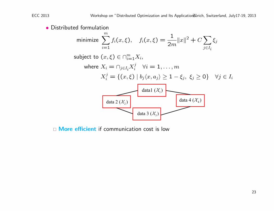
• Distributed formulation

minimizem∑i=1

fi(x, ξ), fi(x, ξ) =1

2m‖x‖2 + C

∑j∈Ii

ξj

subject to (x, ξ) ∈ ∩mi=1Xi,

where Xi = ∩j∈IiXji ∀i = 1, . . . ,m

Xji = (x, ξ) | bj〈x, aj〉 ≥ 1− ξj, ξj ≥ 0 ∀j ∈ Ii

1data1 ( )!

2data 2 ( )! 4data 4 ( )!

3data 3 ( )!

More efficient if communication cost is low

23


Distributed Optimization in Network: Distributed

Constraints

• Problem information distributed: each node (agent) knows fi and Xi only

• Agents unaware of the network topology, only talk to immediate neighbors

1 1min s.t.f !

2 2min s.t.f !

3 3min s.t.f !4 4min s.t.f !

5 5min s.t.f !

6 6min s.t.f !1

x

2x

3x

6x

5x

4x

( ) ( , ( ))

,

( )

1, m

E k V V

G k V E k

V

!

"

# $

!

• Goal: All agents to cooperatively solve

• min f(x) =m∑i=1

fi(x) s.t. x ∈ X ,m⋂i=1

Xi, Xi = ∩j∈IiXji

24


Previous Work on Distributed Optimization

• Markov incremental algorithms § ¶ ‖

• Distributed subgradient algorithms∗∗ †† ‡‡

• None of them can handle on-line constraints

• All of them use an exact projection on Xi

§B. Johansson, M. Rabi, and M. Johansson, “A simple peer-to-peer algorithm for distributed optimization in sensor networks,”in Proceedings of the 46th IEEE Conference on Decision and Control, Dec. 2007, pp. 4705–4710.¶S. S. Ram, A. Nedic, and V. V. Veeravalli, “Incremental stochastic subgradient algorithms for convex optimization,” SIAM J.

on Optimization, vol. 20, no. 2, pp. 691–717, Jun. 2009.‖J. Duchi, A. Agarwal, M. Johansson, M. Jordan, “Ergodic Mirror Descent,” SIAM Journal on Optimization∗∗K. Srivastava and A. Nedic, “Distributed asynchronous constrained stochastic optimization,” IEEE J. Sel. Topics. Signal

Process., vol. 5, no. 4, pp. 772–790, 2011.††A. Nedic, A. Ozdaglar, and P. Parrilo, “Constrained consensus and optimization in multi-agent networks,” IEEE Transactions

on Automatic Control, vol. 55, no. 4, pp. 922–938, April 2010.‡‡I. Lobel, A. Ozdaglar, and D. Feijer, “Distributed multi-agent optimization with state-dependent communication,”

Mathematical Programming, vol. 129, no. 2, pp. 255–284, 2011.

25


Distributed Random Projection (DRP) Algorithm

• Each agent i maintains an estimate sequence xi(k).

1x

2x

3x

6x

5x

4x

1 11 1 12 2

14 4 16 6

( ) ( ) ( ) ( ) ( )

( ) ( ) ( ) ( )

v k w k x k w k x k

w k x k x k x k

! "

" "

12 ( )w k

14 ( )w k

16 ( )w k

11( )w k

• Initialize xi(0), for i ∈ V . For k ≥ 0, each agent i does

1. Mixing vi(k) =m∑j=1

wij(k)xj(k)

2. Gradient update vi(k) = vi(k)− αk∇fi(vi(k))

3. Projection A random variable Ωi(k) ∈ Ii is drawn, and a component XΩi(k)i of

Xi =⋂j∈Ii

Xji is used for projection.

xi(k + 1) = ΠX

Ωi(k)i

[vi(k)]

26


Distributed Mini-Batch Random Projection (DMRP)• What if X〉 consists of 104 hyperplanes?

• 100 samples will provide a better approximation than a single sample

• Initialize xi(0), for i ∈ V . For k ≥ 0, each agent i does the following

1. Mixing vi(k) =∑m

j=1wij(k)xj(k)

2. Gradient update ψ0i (k) = vi(k)− αk∇fi(vi(k))

3. Projections A batch of b independent random variables Ωri(k) ∈ Ii,

r = 1, . . . , b is drawn. The components XΩ1i

(k)

i , . . . , XΩbi(k)

i of Xi =⋂j∈Ii

Xji

are used for sequential projections.

ψri (k) = ΠX

Ωri(k)

i

[ψr−1i (k)], for r = 1, . . . , b

xi(k + 1) = ψbi(k)

( )iv k 1( )i ky

2 ( )i ky

0 ( ) ( ) ( ( ))i i k i ik v k f v ky a= - Ñ

27


Almost Sure Convergence of DRP and DMRP

• Notations

f∗ = minx∈X

f(x), X∗ = x ∈ X | f(x) = f∗

f(x) =m∑i=1

fi(x), X = ∩mi=1Xi

Proposition 1

Let∑∞

k=0 αk =∞ and∑∞

k=0 α2k <∞.

Assume that the problem has a nonempty optimal set X∗.

Then, with typical assumptions, the iterate sequences xi(k), i = 1, . . . ,m,

generated by DRP (or DMRP) algorithm converge almost surely to some (common

random) optimal point x? ∈ X∗, i.e.,

limk→∞

xi(k) = x? for all i = 1, . . . ,m a.s.

28


Assumptions on the Functions fi and Sets Xji

Assumption 1

(a) The sets Xji , j ∈ Ii are closed and convex for every i.

(b) Each function fi : Rd → R is convex.

(c) The functions fi, i ∈ V , are differentiable and have Lipschitz gradients with a

constant L over Rd,

‖∇fi(x)−∇fi(y)‖ ≤ L‖x− y‖ for all x, y ∈ Rd.

(d) The gradients ∇fi(x) are bounded over the set X, i.e., there exists a constant Gf

such that

‖∇fi(x)‖ ≤ Gf for all x ∈ X and all i.

• Assumption 1(d) is satisfied, for example, when X is compact.

29


Assumption on the Set Process Ωi(k)

Assumption 2: Set Regularity

For all i, there exists a constant c > 0 such that

dist2(x,X) ≤ cE[dist2(x,X

Ωi(k)i )

]for all x ∈ Rd.

• This is satisfied when

• Each set Xji is given by a linear (in)equality.

• X has a nonempty interior.

!( )i k

i

!!

( )j

j

k!

!

30


Assumptions on the Network (V,E(k))

Assumption 3 For all k ≥ 0,

Network Connectivity

∃Q > 0 such that the graph(V,⋃`=0,...,Q−1E(k + `)

)is strongly connected.

Doubly Stochasticity

(a) [W (k)]ij ≥ 0 and [W (k)]ij = 0 when j 6∈ Ni(k),

(b)∑m

j=1[W (k)]ij = 1 for all i ∈ V ,

(c) There exists a scalar η ∈ (0,1) such that [W (k)]ij ≥ η when j ∈ Ni(k),

(d)∑m

i=1[W (k)]ij = 1 for all j ∈ V .

• Network is sufficiently connected.

• Each agent is equally influencing every other agent.

31


Simulation ResultsDrSVM: D(M)RP applied on SVM

• Three text classification data sets

2*Data set Statistics

n d s

astro-ph 62,369 99,757 0.08%

CCAT 804,414 47,236 0.16%

C11 804,414 47,236 0.16%

• Experimental set-up

• 80% for training (equally divided among agents), 20% for testing

• Stopping criteria

First run centralized random projection algorithm with b = 1

Set tacc as the test accuracy of the final solution

Limit the total number of iterations

• Stepsize: αk = 1k+1

, Weights: wij(k) = 1|Ni(k)|

32


Simulation Results

• Table shows the number of iterations for all agents to reach the target accuracy tacc

• Graph topologies = clique, 3-regular expander graph

• Batch sizes b = 1, 100, 1000

• Number of agents m = 2, 6, 10

• Maximum iteration = 20,000Data set tacc b m = 2 Clique 3-regular expander

m = 6 m = 10 m = 6 m = 10

astro-ph 0.95 1 1,055 695 697 695 -

100 11 8 11 11 11

1000 2 2 2 2 2

CCAT 0.91 1 752 511 362 517 -

100 11 10 8 10 8

1000 2 3 2 3 3

C11 0.97 1 1,511 1,255 799 1,226 -

100 16 17 12 17 15

1000 2 2 2 2 2

When m = 10 each agent gets about 1,200 data points for astro-ph, and

about 16,000 data points for CCAT and C11

33


Simulation Results

• Repeated 100 times for the column: clique, m = 10

Data set b Clique, m = 10 µ σ 95% confidence

3*astro-ph 1 697 622.7 54.7 [611.8 633.5]

100 11 9.9 1.2 [9.7 10.1]

1000 2 2.1 0.2 [2.0 2.1]

3*CCAT 1 362 441.0 44.8 [432.1 449.9]

100 8 8.2 0.9 [8.0 8.3]

1000 2 2.5 0.5 [2.4 2.5]

3*C11 1 799 1126.4 181.1 [1090.5 1162.3]

100 12 15.5 2.4 [15.1 16.0]

1000 2 3.1 0.7 [3.0 3.3]

• The algorithm is more reliable for larger b

34


Simulation Results - astro-ph: Convergence to f∗

0 200 400 600 800 100010−2

10−1

100

iteration

f(x)

CentralizedDistributed m=10

Compares f(x) when m = 1 (centralized) and m = 10 with b = 1

35


Proof Sketch: Part I

Lemma 1: Projection Error

Let Assumption 1-3 hold. Let∑∞

k=0 α2k <∞.

Then,∞∑k=0

dist2(vi(k), X) <∞ for all i a.s.

• Define zi(k) = ΠX[vi(k)]. This also means

limk→∞

‖vi(k)− zi(k)‖ = 0 for all i a.s.

!1

1 1

j

j I!

" !! !

2

2 2

j

j I!

" !! !

( )1

v k( )

2v k

36


Proof Sketch: Part II

Lemma 2: Disagreement Estimate

Let Assumption 3 hold (network). Consider the iterates generated by

xi(k + 1) =m∑j=1

[W (k)]ijxj(k) + ei(k) for all i.

Suppose ∃ a sequence αk such that∑∞

k=0 αk‖ei(k)‖ <∞ for all i.

Then, for all i, j,∞∑k=0

αk‖xi(k)− xj(k)‖ <∞.

• Since vi(k) =∑m

j=1[W (k)]ijxj(k), we can define ei(k) = xi(k + 1)− vi(k).

•∑∞

k=0 αk‖ei(k)‖ <∞ from Lemma 1.

!1

1 1

j

j I!

" !! !

2

2 2

j

j I!

" !! !

( )1

x k

*!

( )2

x k

37


Proof Sketch: Part III

!

1

1 1

j

j I!

" !! !2

2 2

j

j I!

" !! !

( )1

x k ( )2

x k

*!

Convergence results (Robbins and Siegmund 1971)

Let vk, uk, ak and bk be sequences of non-negative random variables such that

E[vk+1|k] ≤ (1 + ak)vk − uk + bk for all k ≥ 0 a.s.,where k denotes the collection v0, . . . , vk, u0, . . . , uk, a0, . . . , ak and b0, . . . , bk.

Also, let∑∞

k=0 ak <∞ and∑∞

k=0 bk <∞ a.s.

Then, we have limk→∞ vk = v for a random variable v ≥ 0 a.s., and∑∞

k=0 uk <∞ a.s.

38


Proof Sketch: Part III

Basic Iterate Relation and Convergence

Let Assumption 1-3 hold. Let∑∞

k=0 αk =∞ and∑∞

k=0 α2k <∞. For any x? ∈ X∗, we

have

E

[m∑i=1

‖xi(k + 1)− x?‖2 | Fk

]≤ (1 +Aα2

k)m∑i=1

‖xi(k)− x?‖2 +mBα2kG

2f

− 2αk(f(z(k))− f∗) + 4αkGf

m∑i=1

‖vi(k)− v(k)‖,

where z(k) = 1m

∑mi=1 zi(k) with zi(k) = ΠX[vi(k)]. Hence,

∑mi=1 ‖xi(k)− x?‖2

is

convergent for every x? ∈ X∗, and∞∑k=0

αk(f(z(k))− f∗) <∞.

From Lemma 1-2 and the continuity of f , we have

limk→∞

xi(k) = x? for all i a.s.

39


Removal of Doubly Stochastic Weight AssumptionThe subgradient-push method

Every node i maintains auxiliary vector variables xi(t),wi(t) in Rd, as well as an auxiliary

scalar variable yi(t), initialized as yi(0) = 1 for all i. These quantities will be updated by

the nodes according to the rules,

wi(t+ 1) =∑

j∈N ini

(t)

xj(t)

dj(t),

yi(t+ 1) =∑

j∈N ini

(t)

yj(t)

dj(t),

zi(t+ 1) =wi(t+ 1)

yi(t+ 1),

xi(t+ 1) = wi(t+ 1)− α(t+ 1)gi(t+ 1), (1)

where gi(t+ 1) is a subgradient of the function fi at zi(t+ 1). The method is initiated

with wi(0) = zi(0) = 1 and yi(0) = 1 for all i. The stepsize α(t + 1) > 0 satisfies

40


the following decay conditions∞∑t=1

α(t) =∞,∞∑t=1

α2(t) <∞, α(t) ≤ α(s) for all t > s ≥ 1. (2)

We note that the above equations have simple broadcast-based implementation: each

node i broadcasts the quantities xi(t)/di(t), yi(t)/di(t) to all of the nodes in its

out-neighborhood, which simply sum all the messages they receive to obtain wi(t + 1)

and yi(t + 1). The update equations for zi(t + 1),xi(t + 1) can then be executed

without any further communications between nodes during step t.

We note that we make use here of the assumption that node i knows its out-degree di(t).

41


Convergence

Our first theorem demonstrates the correctness of the subgradient-push method for an

arbitrary stepsize α(t) satisfying Eq. (2).

Theorem 1 Suppose that:

(a) The graph sequence G(t) is uniformly strongly connected with a self-loop at every

node.

(b) Each function fi(z) is convex and the set Z∗ = arg minz∈Rd

∑mi=1 fi(z) is nonempty.

(c) The subgradients of each fi(z) are uniformly bounded, i.e., there is Li <∞ such that

‖gi‖2 ≤ Li for all subgradients gi of fi(z) at all points z ∈ Rd.

Then, the distributed subgradient-push method of Eq. (1) with the stepsize satisfying the

conditions in Eq. (2) has the following property

limt→∞

zi(t) = z∗ for all i and for some z∗ ∈ Z∗.

42


Convergence Rate

Our second theorem makes explicit the rate at which the objective function converges to

its optimal value. As standard with subgradient methods, we will make two tweaks in

order to get a convergence rate result:

(i) we take a stepsize which decays as α(t) = 1/√t (stepsizes which decay at faster

rates usually produce inferior convergence rates),

(ii) each node i will maintain a convex combination of the values zi(1), zi(2), . . . for

which the convergence rate will be obtained.

We then demonstrate that the subgradient-push converges at a rate of O(ln t/√t). The

result makes use of the matrix A(t) that captures the weights used in the construction of

wi(t+ 1) and yi(t+ 1) in Eq. (1), which are defined by

Aij(t) =

1/dj(t) whenever j ∈ N in

i (t),

0 otherwise.(3)

43


Convergence Rate

Theorem 2 Suppose all the assumptions of Theorem 1 hold and, additionally, α(t) =

1/√t for t ≥ 1. Moreover, suppose that every node i maintains the variable zi(t) ∈ Rd

initialized at time t = 1 to zi(1) = zi(1) and updated as

zi(t+ 1) =α(t+ 1)zi(t+ 1) + S(t)zi(t)

S(t+ 1),

where S(t) =∑t−1

s=0 α(s+ 1). Then, we have that for all t ≥ 1, i = 1, . . . , n, and any

z∗ ∈ Z∗,

F (z(t))− F (z∗) ≤n

2

‖x(0)− z∗‖1√t

+n

2

(∑ni=1Li

)2

4

(1 + ln t)√t

+16

δ(1− λ)

(n∑i=1

Li

)∑nj=1 ‖xj(0)‖1√t

+16

δ(1− λ)

(n∑i=1

L2i

)(1 + ln t)√

t

where

x(0) =1

n

n∑i=1

xi(0),

and the scalars λ and δ are functions of the graph sequence G(1), G(2), . . . , which

have the following properties:

44


(a) For any B-connected graph sequence with a self-loop at every node,

δ ≥1

nnB,

λ ≤(

1−1

nnB

)1/(nB)

.

(b) If each of the graphs G(t) is regular then

δ = 1

λ ≤ min

(1−

1

4n3

)1/B

,maxt≥1

√σ2(A(t))

where A(t) is defined by Eq. (3) and σ2(A) is the second-largest singular value of a

matrix A.

Several features of this theorem are expected: it is standard for a distributed subgradient

method to converge at a rate of O(ln t/√t) with the constant depending on the

S.S. Ram, A. Nedic, and V.V. Veeravalli, ”Distributed Stochastic Subgradient Projection Algorithms for ConvexOptimization,” Journal of Optimization Theory and Applications,147 (3) 516–545, 2010

J.C. Duchi, A. Agarwal, and M.J. Wainwright, ”Dual Averaging for Distributed Optimization: Convergence Analysis andNetwork Scaling,” IEEE Transactions on Automatic Control, 57(3) 592–606, 2012

45


subgradient-norm upper bounds Li, as well as on the initial conditions xi(0). Moreover,

it is also standard for the rate to involve λ, which is a measure of the connectivity of the

directed sequence G(1), G(2), . . .; namely, the closeness of λ to 1 measures the speed at

which a consensus process on the graph sequence G(t) converges.

However, our bounds also include the parameter δ, which, as we will later see, is a measure

of the imbalance of influences among the nodes. Time-varying directed regular networks

are uniform in influence and will have δ = 1, so that δ will disappear from the bounds

entirely; however, networks which are, in a sense to be specified, non-uniform will suffer a

corresponding blow-up in the convergence time of the subgradient-push algorithm.

The details are in:

AN and Alex Olshevsky, ”Distributed optimization over time-varying directed graphs,”

http://arxiv.org/abs/1303.2289

46

Documents

First-order methods for distributed in-network optimizationautomatica.dei.unipd.it/tl_files/utenti/lucaschenato/ECC13_Workshop/ECC2013Workshop...First-order methods for distributed