First Nature vs. Second Nature Causes: Industry Location

and Growth in the Presence of an Open-Access Renewable Resource

Rafael González-Val1

Fernando Pueyo2

1 Universidad de Barcelona & Instituto de Economía de Barcelona

2 Universidad de Zaragoza, Departamento de Análisis Económico

Abstract: In this paper we present a model integrating characteristics of the New

Economic Geography, the theory of endogenous growth and the economy of natural

resources. This theoretical framework enables us to study explicitly the effect of “first

nature causes” in the concentration of economic activity, more specifically, the

consequences of an asymmetrical distribution of natural resources. The natural resource

we consider appears as a localized input in one of the two countries, giving firms

located in that country a cost advantage. In this context, after a decrease in transport

costs, firms decide to move to the country with the greatest domestic demand and

market size, where they can take more advantage of increasing returns, despite the cost

advantage of locating in the South, due to the presence of the natural resource.

Keywords: industrial location, endogenous growth, renewable resource,

geography

JEL: F43, O30, Q20, R12.

Corresponding address:

Dpto. de Análisis Económico, Universidad de Zaragoza

Facultad de CC. Económicas y Empresariales

Gran Vía 2, 50005 Zaragoza (Spain)

E-mail: fpueyo@unizar.es

1

1. Introduction

There are many factors influencing the distribution of economic activity. It is

traditional to distinguish between characteristics linked to the physical landscape, such

as temperature, rainfall, access to the sea, the presence of natural resources or the

availability of arable land, and factors relating to human actions and economic

incentives (for example, scale economies or knowledge spillovers). The first group of

factors, related to natural geographical circumstances, are called “first nature causes”,

and the second group are called “second nature causes”.

A great deal of effort has been dedicated to researching the influence of second

nature causes, especially after the pioneering work of Krugman (1991), who

demonstrated how economic forces (increasing returns and transport costs) determine

the distribution of activity. However, the models of New Economic Geography are

usually based on the assumption that the space is homogenous, thus controlling the first

nature causes. This means that less work has been invested in the theoretical study of

the effect of first nature causes, even though many empirical studies demonstrate their

important influence on economic growth and the concentration of economic activity.

For the case of the United States, Ellison and Glaeser (1999) state that natural

advantages, such as the presence of a natural harbour or a particular climate, can explain

at least half of the observed geographic concentration. Glaeser and Shapiro (2003) find

that in the 1990s people moved to warmer, dryer places. Black and Henderson (1998)

conclude that the extent of city growth and mobility are related to natural advantages, or

geography. Beeson et al. (2001) show that access to transport networks, either natural

(oceans) or produced (railroads) was an important source of growth during the period

1840-1990, and that climate is one of the factors promoting population growth. And

Mitchener et al. (2003) find that some geographical characteristics account for a high

proportion of the differences in productivity levels between American states.

The aim of this paper is to provide a theoretical model which enables us to

analyse the influence of one of the first nature causes, the presence of natural resources,

on the concentration of economic activity and growth. To do this we will build a model

in which firms can choose to locate in one of two countries which trade with each other,

which we will call North and South. This model integrates characteristics of the New

Economic Geography, the theory of endogenous growth and the economy of natural

resources.

2

We will follow the model developed by Martin and Ottaviano (1999), which

combines a model of endogenous growth similar to that of Romer (1990), and

Grossman and Helpman (1991), with a geographical framework like that of Helpman

and Krugman (1985), and Krugman (1991). Economic growth is supported by an

endogenous framework with national spillovers in innovation, causing research

activities to take place in a single country, and thus, the greater the industrial

concentration in that country, the higher the economic growth rate.

To this model, we add an open access renewable natural resource, used by firms

as a productive input. This introduces an additional element that conditions firms’

decisions about whether to locate in the North or in the South, besides the traditional

home market effect and the existence of trade costs. The relative importance of these

three forces determines a non-symmetrical location of firms. The industrial geography

here relates to the natural resource in two ways. First, the natural resource is located in

only one of the two countries, namely, the South. And, second, the international trade of

the natural resource is subject to a transport cost.

There are other theoretical models which study how the presence of natural

resources affects international trade, focusing on factors such as comparative

advantages and relative prices (Brander and Taylor, 1997a, 1997b, 1998a, 1998b), or

differences in property rights of the resources (Chichilnisky, 1994). This paper proposes

a different approach, as the natural resource has an influence not only on international

trade, but also on the distribution of firms among countries, which is endogenously

determined. In turn, the distribution of economic activity also affects the equilibrium

stock of the natural resource.

The following results are obtained. After a decrease in any of the transport costs,

firms decide to move to the country with the greatest domestic demand and market size.

Despite the cost advantage of locating in the South due to the presence of the resource,

firms prefer to move to the North, the rich country, where they can take more advantage

of increasing returns. In turn, concentration improves the economic growth rate, given

the national nature of the spillovers. The concentration of firms in the North also has a

positive effect on the stock of the natural resource, which increases. This means that in

the framework of our model, second nature causes (the home market effect), acting

centripetally, have greater weight in firm decisions than the advantages of natural

geographic circumstances (first nature causes) which act centrifugally.

3

However, the South can increase the importance of the first nature cause by

introducing public policies to reinforce the cost advantage of the resource’s presence for

firms located in the South. We will consider two public policies: imposing restrictions

on the international trade of the resource and promoting a technological change to a

technology which uses the resource more intensively. In both cases, after such policies

the South attracts firms from the North, producing decreases in the growth rate and in

the stock of the natural resource in equilibrium. The effect on welfare remains

undetermined.

The next section presents the basic characteristics of the theoretical model.

Section 3 describes the market equilibrium of differentiated goods, with special

attention given to the distribution of firms in the equilibrium. Section 4 describes the

natural resource market and solves the corresponding equilibrium. Section 5 determines

the steady state growth rate, which depends on geography, and also shows how

economic growth in turn influences geography through income inequality. Once the

general equilibrium is described, section 6 analyses the effect of changes in

differentiated goods’ and resource’s transport costs. These transport costs can also be

interpreted in terms of public policies, as seen in section 7. Finally, the paper ends with

the main conclusions.

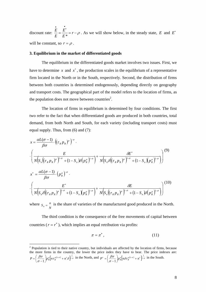
2. The model

The diagram in Figure 1 describes schematically how the model works. We will

consider two countries, North and South, which trade with each other. Both are identical

except for their initial level of capital, 0K in the North and ∗0K in the South, and the

presence of a natural resource only in the South. Let us suppose that the North has a

higher initial income level, such that ∗> 00 KK . Both countries are inhabited by

representative households playing the part of consumers, workers and researchers.

There are L households, both in the North and in the South. Labour is mobile between

sectors but immobile between countries.

Given that the model is nearly symmetrical, we will focus on describing the

economy of the North (an asterisk denotes the variables corresponding to the South).

The preferences are instantaneously nested CES, and intertemporally CES, with an

elasticity of intertemporal substitution equal to the unit:

4

[ ]∫∞ ⋅−−=0

1)()(log dtetYtDU tραα , 10 <<α , (1)

where ρ is the intertemporal discount rate, Y is the numerary good and D is a

composite good which, in the style of Dixit and Stiglitz, consists of a number of

different varieties:

⎟⎠⎞

⎜⎝⎛ −

=

−

⎥⎥⎦

⎤

⎢⎢⎣

⎡= ∫ σσ

11

1

)(

0

11)()(

tN

i i ditDtD , 1>σ . (2)

N is the total number of varieties available, both in the North and the South. σ is the

elasticity of substitution between varieties, and is also the demand price elasticity of the

demand for each variety (assuming that N is high enough). Growth comes from an

increase in the number of varieties. Note that the natural resource does not appear

explicitly in the structure of individual preferences, meaning that it lacks value for them

(but it might have social value, as a planner might exist who decides to maintain a

minimum level). This assumption is restrictive, but has a double justification. First, the

indirect utility function is very difficult to analyse even without including the natural

resource (see section 7). Including it would give rise to more indeterminacy (although,

as we will see below, the resource does appear in the indirect utility function indirectly

through its price). And second, individuals cannot move between countries. This means

that they cannot react in any way to changes in the stock of the resource, and so

introducing it into its utility function makes no sense.

The value of per capita expenditure E in terms of the numerary Y is:

EYdjDpdiDpnj jjni ii =++ ∫∫ ∗∈

∗

∈τ . (3)

The number of manufactured goods produced in each country, n and ∗n , is

endogenous, with ∗+= nnN . There is a transport cost ( )1>τ that affects international

trade between the two countries. Also, international trading of the natural resource from

South to North is also subject to a transport cost Rτ . τ and Rτ represent iceberg-type

costs, as in Samuelson (1954), and reflect the part of the good which is lost in transit.

The transport costs operate according to the following schema:

5

Thus, only 11 <−τ of each unit of differentiated variety sent from the other

country is available for consumption. Similarly, the North incurs an additional transport

cost deriving from the natural resource (only 11 <−Rτ of each unit of the natural resource

sent from the South can be used) which the South does not bear. Decreases in τ or Rτ

facilitate trade. From here we will assume that ττ ≤R ; in other words, it is less costly

or, at best, the same in terms of transaction costs to send units of the natural resource

than the differentiated good1. Meanwhile, the numerary good is not subject to any

transaction cost.

The numerary good is produced using only labour, subject to constant returns in

a perfectly competitive sector. As labour is mobile between sectors, the constant returns

in this sector tie down the wage rate w in each country at each moment. We assume

throughout the paper that the parameters of the model are such that the numerary is

produced in both countries, that is, that the total demand for the numerary is big enough

so as not to be satisfied with its production in a single country. In this way, wages are

maintained constant and identical in both countries. A unit of labour is needed to

produce a unit of Y , so free competition in the labour market implies that 1=w in both

countries.

The differentiated goods are produced with identical technologies, in an industry

with monopolistic competition with increasing scale returns in the production of each

1 The results are maintained even when transport cost for the resource is higher than that of the differentiated good, as long as the difference is not too great (it is a sufficient condition).

6

variety. To begin to produce a variety of a good, a unit of capital is needed; this fixed

cost )(FC is the source of the scale economies. Labour )(L and natural resource )(R

combine through a Cobb-Douglas type technology, μμiii RLx −= 1 , with a proportion

)1,0(∈μ for the natural resource that represents how intensive the technology is in the

use of the resource. This makes firm costs different if they are located in the North or

South. If β represents the variable cost, the costs function of a representative firm in

the North is as follows: qxFCc ii β+= , while that of a firm in the South, which does

not have to bear transport costs for the natural resource ( )Rτ , is: ∗+= qxFCc ii β ,

where q and ∗q are the price indexes of the producers: ( )μμ τ RR pwq −= 1 , and μμRpwq −∗ = 1 , and Rp is the market price of the natural resource. Therefore, firms in the

South enjoy a competitive advantage in costs derived from the presence of the natural

resource in its territory.

The standard rule of monopolistic competition determines the price of any variety

produced either in the North or the South. The difference in costs implies that these

prices are different: ( )μτσσβ RR pp ⎟

⎠⎞

⎜⎝⎛

−=

1 in the North and μ

σσβ Rpp ⎟

⎠⎞

⎜⎝⎛

−=∗

1 in the

South, where we have taken into account that 1=w in both countries. Specifically, the

price for any variety fixed by firms in the North is higher than the price fixed by firms

in the South due to the additional transport costs for the natural resource that they bear

( ∗> pp as 1>Rτ ).

The operating profits of the firms are also different depending on the country where

they are located:

( )μτσββπ RRiiiii pxqpxpxp ⎟

⎠⎞

⎜⎝⎛

−=−=

1)()( (4)

in the North, and

μ

σββπ Riiiii pxqpxpxp ⎟⎟

⎠

⎞⎜⎜⎝

⎛−

=−=∗

∗∗∗∗∗∗∗

1)()( (5)

in the South, where x and ∗x are the production scale of a representative firm in the

North and in the South, respectively.

7

In order to produce a new variety a previous investment is required, either in a

physical asset (machinery) or an intangible one (patent). The concept of capital used in

this paper corresponds to a mixture of both types of investment. We assume that each

new variety requires one unit of capital. Thus, the value of any firm is the value of its

unit of capital. The total number of varieties and firms is determined by the aggregate

stock of capital at any given time: ∗∗ +=+= KKnnN . Once the investment is made,

each firm produces the new variety in a situation of monopoly and chooses where to

locate its production, as there are no costs of relocating the capital from one country to

the other. Unlike firms, households (workers/researchers/consumers) are immobile, so

their income is geographically fixed, although the firms can move. In other words, if a

firm owner decides to locate production in the country where he does not reside, he

repatriates the profits.

Finally, we assume there is a safe asset which pays an interest rate r on units of

the numerary, whose market is characterized by freedom of international movements

( )∗= rr .

Solving the first order conditions of the problem of the consumer in the North

we obtain the demands for each variety produced in the North ( )iD , in the South ( )jD ,

and for the numerary good:

( )( )( )( ) ( )( )σμσμ

σμ

δτ

ατβσσ

−∗−

−

+⋅

−=

11

1

RRR

RRi

pnpn

EpD (6)

( )( )( ) ( )( )σμσμ

σμσ

δτ

ατβσσ

−∗−

−−

+⋅

−=

11

1

RRR

Rj

pnpn

EpD (7)

EY )1( α−= (8)

where στδ −= 1 is a parameter between 0 and 1 that measures the openness of trade:

1=δ represents a situation in which transport costs do not exist, while if 0=δ trade

would be impossible due to the high transaction costs.

The intertemporal optimization of consumers implies that the growth rate of

expenditure is given by the difference between the interest rate and the intertemporal

8

discount rate: *

E E rE E

ρ

••∗

= = − . As we will show below, in the steady state, E and ∗E

will be constant, so ρ=r .

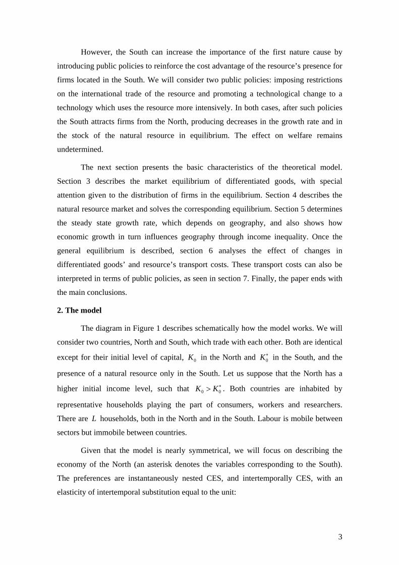
3. Equilibrium in the market of differentiated goods

The equilibrium in the differentiated goods market involves two issues. First, we

have to determine x and ∗x , the production scales in the equilibrium of a representative

firm located in the North or in the South, respectively. Second, the distribution of firms

between both countries is determined endogenously, depending directly on geography

and transport costs. The geographical part of the model refers to the location of firms, as

the population does not move between countries2.

The location of firms in equilibrium is determined by four conditions. The first

two refer to the fact that when differentiated goods are produced in both countries, total

demand, from both North and South, for each variety (including transport costs) must

equal supply. Thus, from (6) and (7):

( )( )

( )( ) ( ) ( )( ) ( )( ) ( )( )( )⎟⎟

⎠

⎞

⎜⎜

⎝

⎛

−++

−+⋅

⋅⋅−

=

−−

∗

−−

−

σμσμσμσμ

σμ

τδ

δ

δτ

τβσσα

111111

)1(

RnRRnRnRRn

RR

pSpSN

E

pSpSN

E

pLx

(9)

( )

( )( ) ( )( )( ) ( )( ) ( ) ( )( )⎟⎟

⎠

⎞

⎜⎜

⎝

⎛

−++

−+⋅

⋅⋅−

=

−−−−

∗

−∗

σμσμσμσμ

σμ

δτ

δ

τδ

βσσα

111111

)1(

RnRRnRnRRn

R

pSpSN

E

pSpSN

E

pLx

(10)

where NnSn = is the share of varieties of the manufactured good produced in the North.

The third condition is the consequence of the free movements of capital between

countries ( ∗= rr ), which implies an equal retribution via profits:

∗= ππ , (11)

2 Population is tied to their native country, but individuals are affected by the location of firms, because the more firms in the country, the lower the price index they have to bear. The price indexes are:

( )[ ] σσμμ δτσβσ

−∗− +⎟⎠⎞

⎜⎝⎛

−= 1

11

1nnpP RR

in the North, and ( )[ ] σσμμ δτσβσ

−∗−∗ +⎟⎠⎞

⎜⎝⎛

−= 1

11

1nnpP RR

in the South.

9

and, therefore, according to (4) and (5), μτ R

xx∗

= . Finally, the fourth condition, already

mentioned, indicates that the total number of varieties is fixed by the worldwide supply

of capital at each moment:

NKKnn =+=+ ∗∗ . (12)

Solving the system formed by these four equations, we obtain the optimum size

of each firm in equilibrium in the North and in the South:

( ) ( ) μτβσσα −

∗

⋅+

⋅−

= RR pN

EELx )1( , (13)

( ) μ

βσσα −

∗∗ ⋅

+⋅

−= Rp

NEELx )1( . (14)

The equilibrium production scales are different in each country. Locating in the North

implies an additional cost due to the transport of the natural resource, and the firms react

by producing fewer units of the differentiated good that they sell at a higher price. In

turn, this different behaviour is what enables profits obtained in equilibrium to be the

same in both countries.

The proportion of firms (or varieties) in the North (Nn

nS = ) is given by:

( )( )( )δφδ

φδ −−

−⋅−

=R

E

R

En

SSS 11

, (15)

where, in turn, ∗+

=EE

ESE is the participation of the North in total expenditure and

( )σμτφ −= 1RR is a parameter between 0 and 1 of similar interpretation to δ , measuring the

freedom of trade of the natural resource. It is also possible to demonstrate that, as long

as the North has a larger domestic market3 ⎟⎠⎞

⎜⎝⎛ >

21

ES , most firms are located in the

North ⎟⎠⎞

⎜⎝⎛ >

21

nS .

The location of equilibrium of the firms depends on national expenditure –

higher local expenditure or income means a larger domestic market, which attracts more 3 Below it is shown that this condition is always borne out as long as ∗> 00 KK , as we have supposed.

10

firms wanting to take advantage of increasing returns (home market effect) – and the

relationship between the level of openness of trade of differentiated goods ( )δ and of

the natural resource ( )Rφ . The natural resource influences the distribution of firms in

equilibrium via Rφ : the lower the transport cost of the natural resource, the smaller the

advantage for firms located in the South. It is easy to see that ( ) 0>−δφR as long as

ττ ≤R . Given that most firms are concentrated in the North, the home market effect,

which we may identify as a second nature cause, acts centripetally, favouring the

agglomeration of economic activity, while the cost advantage offered by the natural

resource to firms located in the South, the first nature cause, acts centrifugally.

4. Natural resource growth

The South is endowed with a stock of natural resource ( )S , characterized as in

Eliasson and Turnovsky (2004) or in Brander and Taylor (1997a, 1997b, 1998a, 1998b).

This natural resource has some specific characteristics. It is (i) renewable, (ii) open

access, (iii) used only as an input in the production of manufactured goods, and (iv) its

exploitation requires only labour. These four conditions can be considered as restrictive,

but are necessary to keep the model tractable. A natural resource with such

characteristics is, for example, the wood from the forests of the South.

At any point of time, the net change in the stock of the resource is given by

( ) RSGS −=•

, where ( )SG describes the natural growth of the resource and R is the

harvested amount. We assume that the reproduction function G is a concave function

depending on the current stock of the resource, and positive in the interval between S

and S , where S is the minimum viable stock size and S is the maximum amount

which the stock can reach, given physical and natural limitations (for example, available

space). ( )SG is analogous to a production function, with the difference that the rate of

accumulation of the stock is limited. See Brown (2000) for a wider discussion of ( )SG

and its properties.

For simplicity, we fix 0=S and assume that the growth of the resource, ( )SG ,

corresponds to a logistic function:

( ) ⎟⎠⎞

⎜⎝⎛ −=

SSSSG 1γ , 0>γ (16)

11

where γ is the intrinsic growth rate of the resource (the natural growth rate). In the

absence of harvesting ( )0=R , S converges to its maximum sustainable stock level, S .

This function has been widely used in the analysis of renewable resources, and may be

the simplest and most empirically plausible functional form of describing biological

growth in a restricted environment.

The harvest of the natural resource requires economic resources; for the sake of

simplicity, we will assume it requires only labour. We assume that harvesting is carried

out according to the Schaefer harvesting production function:

RS BSLR = , (17)

where RL is the amount of labour used in the renewable resource sector (workers in the

South, where the resource is located), SR is the harvested quantity offered by the

producers and B is a positive constant. If ( )SaRL represents the unit labour requirement

in the resource sector, (17) implies that ( )BSR

LSa S

RLR

1== . It verifies ( ) 0<′ Sa

RL :

labour requirement increases as the stock of the resource decreases.

Production is carried out by profit-maximizing firms operating under conditions

of free entry (perfect competition). Therefore, the price of the resource good must equal

its unit production cost:

BSBS

wwapRLR

1=== . (18)

Both B and w are in terms of the numerary good, so Rp is too. This price incorporates

the assumption of open access to the resource, because the only explicit production cost

is labour. There are no other explicit costs of using the resource4.

The firms in the sector of the differentiated goods demand the natural resource

as an input in the production of their varieties. Applying Shephard’s lemma to the cost

functions we obtain the demand for the natural resource: ( ) 1−⋅ μτμβ RR px for a

representative firm of the North and 1−∗ ⋅ μμβ Rpx for a representative firm of the South.

4 If there were no free access to the resource, another cost would exist deriving from the reduction of the capacity for reproduction of the resource, which relates to Hotelling’s rule. The resource would be exploited only by firms with property rights in a situation which would then not be perfect competition, making the final price greater than the unit cost, and generating additional income.

12

Substituting the equilibrium production levels given by (13) and (14), and aggregating

for the firms in the North (taking into account the transport cost they bear) and in the

South, we obtain the worldwide demand for the resource ( )DR :

( )∗− +⋅−

⋅= EELpR RD

σσαμ )1(1 . (19)

This demand depends on some structural parameters, the price of the resource and world

aggregate income, ( )∗+ EEL .

Replacing in (19) the price set by the producers, given by (18), we obtain the

resource market equilibrium condition, which gives us the equilibrium harvest level R :

( ) ( )∗+⋅−

⋅= EELBSSRσσαμ )1( . (20)

Note that this harvest level R is a function ( )SR that grows with the size of the

stock S . Steady state is reached when the stock evolves to a level in which the harvest

of the natural resource, ( )SR , is equal to its capacity for reproduction, ( )SG , given by

equation 16, meaning that ( ) ( ) 0=−=•

SRSGS . A trivial solution is reached when

0== RS . The other solution is given by:

( )⎥⎦

⎤⎢⎣

⎡+⋅

−⋅−= ∗EELBSS

γσσαμ )1(1~ . (21)

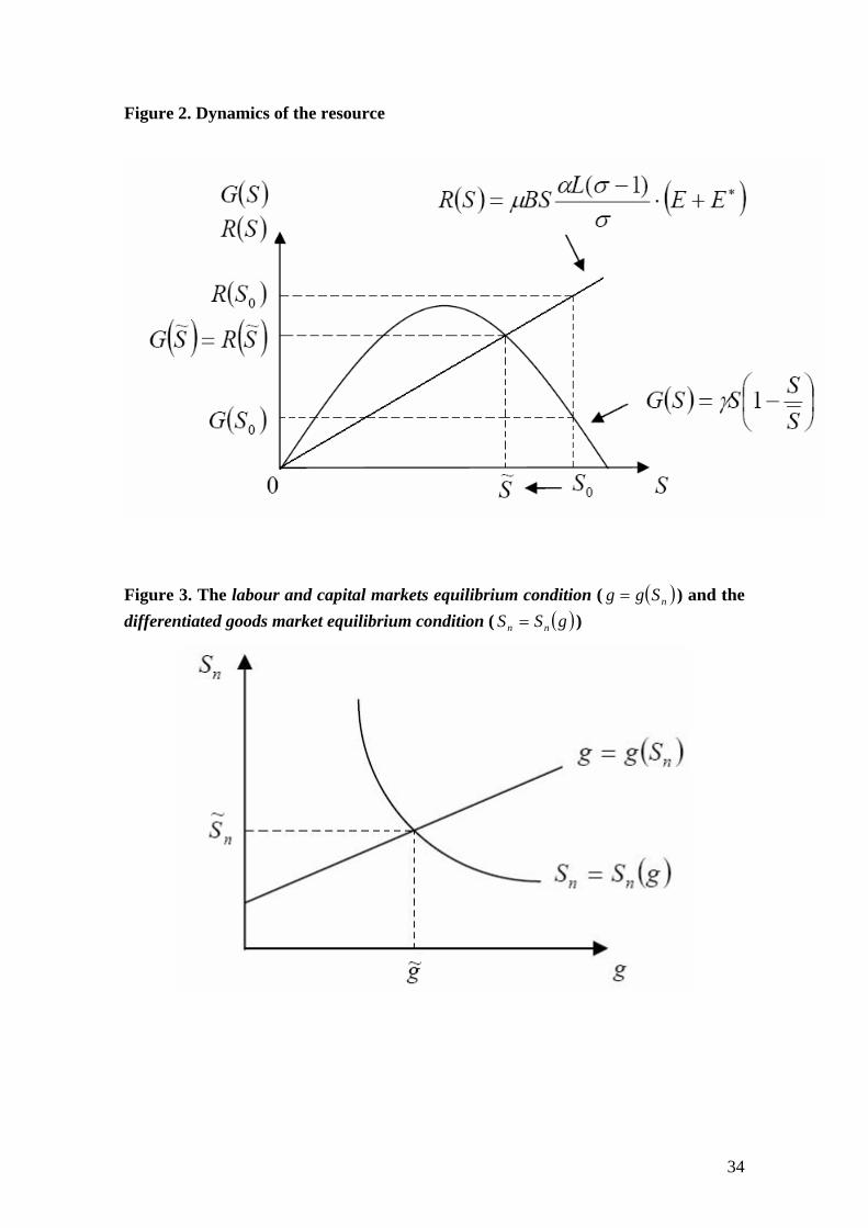
Figure 2 shows how convergence is produced to the steady state level. The

figure illustrates a situation in which at the initial stock 0S the amount harvested,

( )0SR , exceeds natural growth, ( )0SG . The stock then decreases until it reaches the

steady state level S~ . This indicates that, in steady state, the quantity of the resource

used by firms is constant.

The steady state harvest level is obtained by replacing S~ in ( )SR :

( ) ( ) ( )⎥⎦

⎤⎢⎣

⎡+⋅

−⋅−⋅+⋅

−⋅= ∗∗ EELBSEELBSR

γσσαμ

σσαμ )1(1)1(~ . (22)

As shown by Brander and Taylor (1997a), a positive steady state solution exists

if and only if the term between brackets is positive, that is to say, if the condition

13

( )L

EEB γσσαμ <+⋅−

⋅ ∗)1( holds. In this case the solution is globally stable (for any

00 >S ). If such condition is not satisfied the resource would disappear and the unique

possible steady state is 0== RS . Graphically, this condition means that, in the origin,

the slope of the function ( )SR is less than the slope of ( )SG , thus ensuring that they cut

off at some point for positive values of S.

5. Economic growth and income inequality

5.1 Economic growth

We will first examine the growth rate of the economy. Starting from the solution

of the problem of the intertemporal optimization of the consumer, we know that, in

equilibrium, ρ−== ∗

•∗

•

rEE

EE . As the capital flows are free, ∗= rr , and the expenditure

growth rate will be the same in both countries. From (15), this implies that the ratio of

firms producing in the North, nS , is also constant in time, and, therefore, n , ∗n and N

grow at the same constant rate ∗

•∗

••

===nn

nn

NNg .

National spillovers exist in the innovation sector, so that the more firms

producing different manufactured goods are located in the same country, the less costly

is R&D5. This sector follows Grossman and Helpman (1991), with nη being the cost in

terms of labour of an innovation in the North and ∗nη in the South. The immediate

conclusion of this formulation of the sector is that, for reasons of efficiency, research

activity will take place in only one of the two countries: the one with the most firms

producing manufactured goods (which will be the rich country, the North, given that

21

>nS ). No researcher will have any incentive to begin R&D in the other country. This

formulation makes the analytical treatment of the model easier, although the results are

5 This type of knowledge spillovers is closer to the concept of Jacobs (1969) than to that of Marshall-Arrow-Romer (MAR). The empirical evidence for these external effects between different industries in the same geographical unit is documented; see, for example, Glaeser et al. (1992) and Henderson et al. (1995).

14

maintained even if a certain degree of diffusion of the knowledge exists at the

international level (Hirose and Yamamoto, 2007).

The value of the firm is given by the value of its unit of capital. As the capital

market is competitive, this value ( v ) will be given by the marginal cost of innovation,

nNSnv ηη

== , which is therefore decreasing at the rate g , the rate of innovation

( gvv

−=

•

). As the number of varieties increases, the profits of each firm decrease, and

also does its value, which can also be interpreted as the future flow of discounted profits

[ ] ⎟⎠⎞

⎜⎝⎛

−= ∫

∞ −−

t

trsr dssxetv1)()( )()(

σβ , where r represents the cumulative discount factor.

Taking into account the arbitrage condition between the capital market and the safe

asset market, the relation between the interest rate and the value of the capital is given

by 6:

vvvr π+=

•

. (23)

On the other hand, the constraint of world resources, ( ) ( )nLSrEE η+=+ ∗ 2 ,

where the right-hand includes the sum of labour income ( 1=w in the two countries)

and capital returns, implies that worldwide expenditure is constant over time, so that in

steady state ρ=r , as pointed above. Note that this restriction includes only labour and

capital returns; the harvest of the natural resource does not generate additional income

for either of the two countries, as it is an open access resource exploited in a

competitive industry.

Finally, we must take into account the labour market. The world’s labour is

devoted to R&D activities (using only workers from the North), and to the production of

goods. From the latter, a proportion ( )α−1 is dedicated to the production of the

numerary good, and a proportion α to the production of differentiated goods. In turn,

given the Cobb-Douglas technology properties, from the labor used, either directly or

indirectly, in the production of manufactured goods, a proportion μ is used in the

6 This condition is formulated in terms of the profits of the firms in the North ( )π , but applies in the same way to the South because, although the expressions of π and ∗π differ (equations 4 and 5), one of the conditions of equilibrium (equation 11) requires that ∗= ππ .

15

exploitation of the resource (using only workers in the South), and a proportion 1 μ− is

used directly as an input in the production of varieties. Thus, the world labour market

equilibrium condition is given by:

LEELSg

n

2)( =+⎟⎠⎞

⎜⎝⎛ −

+ ∗

σαση . (24)

In steady state (see details in Appendix A), all the variables will grow at a

constant rate. Replacing in (23) the profits obtained in (4), the optimum size of firms in

the equilibrium (13), and considering (24) and that in steady state ρ=r , we obtain the

labour and capital markets equilibrium condition:

( )nn SgSLg =⎟⎠⎞

⎜⎝⎛ −

−⋅= ρσασ

σα

η2 . (25)

where g is the growth rate of K and ∗K (the same for the two countries) in steady

state7. This rate depends on structural parameters of the model ( ρσαη ,,,,L ), but also

on nS (the geography), lineally.

5.2 World income distribution

Secondly, we are interested in how this economic growth rate affects income

inequality between the countries. Remember that we assumed the North to be richer

initially ( ∗> 00 KK ). The per capita income of each country is the sum of labour income

(which, as we have already seen, is the unit), plus the capital income, which is r times

the value of per capita wealth. Thus, it will be L

KvL

KvrE ρ+=+= 11 for any

individual in the North. If we replace v from the arbitrage condition between the

capital market and the safe asset market (23), the equilibrium profits (4), and the

optimum production scale (13), it is possible to express Northern expenditure as a

function of g :

( ) gS

E K

σρασαρ

+−+=

21 , (26)

7 Again the results are presented in terms of the variables of the North (π and x ). Using ∗π and ∗x the same result is obtained (the steady state economic growth rate is the same for the two countries), taking into account that in equilibrium ∗= ππ , meaning that

μτ R

xx∗

= .

16

where ∗+=

KKKSK is the share of capital owned by the individuals in the North, that

remains constant because K and ∗K grow at the same rate g in the steady state.

Similarly, for the South:

( )( ) g

SE K

σρασαρ

+−−

+=∗ 121 . (27)

We have previously defined the ratio ∗+

=EE

ES E , which represents the

participation of the North in total income or expenditure. Replacing the expressions (26)

and (27) we obtain:

( ) ( )( )g

SgS K

E +−++

⋅=ρσαρρσ 12

21 . (28)

If, as we have supposed, the North is richer and 21

>KS , then 21

>ES . However, the

relationship of ES with the economic growth rate is negative: as the number of varieties

increases, the value of the capital is reduced, and, as the North individuals own more

capital, the income difference is reduced in relative terms.

Finally, to carry out the analysis of the next section, we need to relate the geography

)( nS with the growth rate g . To do this, we replace (28) in (15), obtaining the

differentiated goods market equilibrium condition, indicating the distribution of firms

for each value of g :

( ) ( )( ) ( ) ( ) ( )( ) ( )[ ]gSS

gS

gS Enk

RRRR

n =⎥⎦

⎤⎢⎣

⎡+−

⋅−+−+−⋅−

=ρσ

αρφδδφδ

δφφδ12

1211

21

22 . (29)

5.3. Equilibrium

We have obtained two equations, (25) and (29), representing, respectively, the

labour and capital markets equilibrium condition and the differentiated goods market

equilibrium condition. These functions relate the growth rate with the spatial

distribution of firms, and define the equilibrium values of these variables. Since the

algebraic solution is not easy, we follow a graphical approach.

The function ( )nSgg = is linear and increasing: given the nature of the

technological spillovers (national), the greater the concentration of firms, the lower the

17

costs of innovation and the higher the growth rate. The function ( )gSS nn = is convex

and decreasing8. Remember that this equation incorporates the inequality of income,

( )[ ]gSSS Enn = , and that this decreases as g increases via the reduction of

monopolistic profits of firms. At the same time, as the differences in income vanish,

industrial concentration and the market size of the rich country decrease due to the

home market effect.

These functions are represented in Figure 3. The intersection point determines

the steady state location of firms as well as the growth rate of the economy.

6. Effects of reducing trade costs

As we explained in the introduction, the purpose of this paper is explicitly to

study the effect of first nature causes on the concentration of economic activity,

analyzing one of the possible natural geographical characteristics, the role which may

be played by a natural resource.

Starting from the equilibrium situation, a change in differentiated goods’ or

natural resource’s transport cost will lead to changes in the distribution of firms. Firms

move according to two types of incentives: the North attracts firms thanks to its larger

domestic market, 21

>ES , which we can identify as one of the second nature causes of

concentration of firms, while the first nature causes in our model refer to the advantage

in costs enjoyed by firms in the South thanks to the geographical presence of the natural

resource in its territory.

Variations in any type of transaction cost do not affect the function ( )nSgg = ,

which depends only on the structural parameters of the model. It is the curve

( )gSS nn = which will reflect the changes in transport costs, moving and changing its

slope. We carry out our analysis, first, from the perspective of the effects that

decreasing transport costs have on the industrial localization and the growth rate. Then,

the effect on the equilibrium stock of the resource is analyzed.

8 ( )gSS nn = is convex and decreasing as long as ( ) 0>−δφR . This condition is verified if ττ ≤R , as we have been assuming from the begining. Additionally, ( )δφ −R is greater than zero even when transport cost for the resource is higher than that of the differentiated good, as long as the difference is not too great.

18

6.1 Effects on industrial concentration and economic growth

Decrease in the transport cost of differentiated goods

Let us consider first a decrease in the differentiated goods trading cost: 0<τd .

After differentiating the equations (25) and (29), we obtain that 0<τd

dSn , 0<τd

dg and,

thus, both the proportion of firms located in the North and the economic growth rate

increase. This situation is represented in Figure 4.

The decrease in transaction costs enables an easier access to the market of the

other country, so some firms prefer to move to the North (remember that there are no

relocation costs). Despite the cost advantage of locating in the South due to the presence

of the natural resource, firms prefer to move to the North, the rich country and thus the

bigger market, where they can take more advantage of increasing returns. This means

that, in the framework of our model, the home market effect (second nature causes),

acting centripetally, have a greater weight in firm decisions than the advantages of

natural geographic circumstances (first nature causes), which act centrifugally.

In turn, concentration speeds up the economic growth rate, because the more

manufacturing firms are located in the North, the lower the cost of innovation given the

national nature of the spillovers.

Decrease in the transport cost of the resource

If the transport cost of the natural resource decreases, 0<Rdτ , we obtain that

0<R

n

ddSτ

, 0<Rd

dgτ

. Thus, both the proportion of firms located in the North and the

economic growth rate rise: Figure 5 shows this situation. The difference from Figure 4

is that, in this case, the slope of the curve ( )gSS nn = moves upwards rather than

downwards.

The lower transport cost of the natural resource means a loss in the cost

advantage of the firms located in the South, close to the natural resource, over those

located in the North. At the limit, if this transport cost did not exist ( 1=Rτ ) the firms

could not extract any advantage from its location close to the resource and there would

be no relationship between the distribution of natural resource and the economic

19

geography. In other words, as the transport cost of natural resources decreases, the

importance of the first nature cause (in our model, the natural resource) vanishes.

As a consequence of this decrease in relative costs in the North, firms move

from the South to the North, which has a bigger domestic market and greater demand.

Moreover, as the number of firms in the North increases, the cost of research decreases

due to national spillovers, and the economic growth rate increases.

6.2 Effects on the stock of the natural resource

Any variation in the distribution of firms or in the economic growth rate,

whether due to a change in the transport cost of differentiated goods or of the resource,

will have an effect on the stock level of the resource in steady state. That is, changes in

the geographical distribution of firms affect the market of the natural resource.

Let us remember that both the harvest level, given by the resource market

equilibrium condition (equation 20), and the stock of the resource in equilibrium

(equation 21), depend on aggregate world income ( )∗+ EEL . In turn, world income can

be related to nS and g , replacing in (23) the profits obtained in (4) and the optimum

size of firms in the equilibrium (13):

nSgEEL

αρησ )()( +

=+ ∗ . (30)

If we replace this expression of world income in (20) and (21) we obtain:

⎥⎦

⎤⎢⎣

⎡ +⋅

−⋅−=

nSgBSS )()1(1 ρη

γσμ , (31)

( )nS

gBSSR )()1( +⋅−⋅=

ρησμ . (32)

From these expressions we can analyse the effects on the natural resource of the

changes in the distribution of firms. Let us consider changes in the transport costs that

lead to a higher proportion of firms located in the North ( 0>ndS ), that is, reductions in

the transport cost of either the intermediate goods or the natural resource. In turn, given

the national nature of the R&D spillovers, the higher concentration of firms in the North

reduces the cost of innovation and raises economic growth: 0>dg . So, by

20

differentiating (31), we obtain the effect of the reduction in transport costs on the stock

of the natural resource in steady state:

( ) ⎥⎦

⎤⎢⎣

⎡+−⋅

−⋅−= n

nn

dSgS

dgS

BSdS ρηγ

σμ 11)1( .

This expression enables us to identify two opposite effects:

a) Industry localization effect: As the number of firms located in the North increases,

the amount of the resource which is harvested decreases, because the firms in the

North produce less units of differentiated good ( )∗< xx and thus require less

natural resource.

b) Growth effect: As the number of firms in the North increases, the growth rate of

the number of varieties also increases, so that the number of firms grows faster.

More firms require a higher aggregate amount of the natural resource.

However, applying that, from (25), ndSLdgσα

η⋅=

2 , it is possible to obtain a clear sign:

01)1(2 >⎥⎦

⎤⎢⎣⎡−⋅

−⋅−= n

n

dSS

BSdS ρσαη

γσμ ,

indicating that the firms localization effect dominates: more firms in the North means

that less resource is consumed on average, enabling the level of stock to increase in

steady state.

On the other hand, the effect on the harvested amount is not clearly determined.

If we differentiate (32), and replace dg and dS with the expressions obtained earlier,

we have:

02

2)1( 2><⎥

⎦

⎤⎢⎣

⎡−⎟

⎠⎞

⎜⎝⎛ −−= n

n

dSSSS

BdR ρσαησμ .

The sign of the above expression depends on 2SS − , that is, on whether the initial

steady state stock exceeds or not 2S . The same conclusion can be obtained if we

differentiate the function ( )SG (equation 16). Graphically, it depends on whether S~ is

21

on the increasing or decreasing part of ( )SG . Figures 6 and 7 illustrate the two

possibilities.

In Figure 6 we consider the case 2

~ SS > , meaning that 0<dR after the

reduction in transport costs. In this situation, the increasing number of firms in the

North is accompanied by a decrease in the amount harvested. This will be the most

common solution, as it corresponds to situations where the slope of the function ( )SR is

low. From (32), this is the more probable case when the industry is highly concentrated

in the North and/or the technology of the intermediate good firms is not very intensive

in the use of the natural resource.

In contrast, if the function ( )SR is very steep and 2

~ SS < , the amount harvested

increases ( 0>dR ). This case is represented in Figure 7, and corresponds to situations

where, despite consuming more resource, the equilibrium stock increases due to the

high capacity of regeneration of the natural resource on this side of the curve ( )SG .

7. Public policies: How to protect the South’s natural advantage?

In the previous section we analyzed the effects of decreases in transport costs,

obtaining as a result an increase in industrial concentration in the North, the rich

country, and an increase in the growth rate and the stock level of the resource in steady

state. Such lower transport cost of the natural resource meant that the firms of the South

lost some of the cost advantage due to the closer location of the natural resource. That

is, as the transport cost of the resource decreases, the less important this first nature

cause becomes, configured as a centrifugal force, and the more firms concentrate in the

North.

From this point of view, there is not much the South can do faced with a rich

North with the home market effect in its favour, in a context of international transport

costs trending downwards over time, so that sooner or later the cost advantage will

disappear. However, the South can consider some public policies in order to protect the

cost advantage.

22

Restrictions on international trading of the resource

A first route, the most direct, would be to influence Rτ , since higher transport

costs for the resource increase the cost advantage for firms in the South. By modifying

slightly the interpretation of the parameter Rτ , we can consider some ways the South

could protect and even increase the cost advantage given by nature.

Martin and Rogers (1995) posited that the transport costs used in the models of

Economic Geography can alternatively be interpreted as a measure of the quantity and

quality of transport infrastructures, and, thus, can be modified by public policies. From

this point of view, they defined public transport infrastructures as any good or service

provided by the state which can facilitate the connection between production and

consumption. It is evident that transport and communication media can be included

among these trade infrastructures, but there are other non-physical elements, such as the

legal system or the levels of public safety, which have an equally great influence on

trade. Good infrastructures mean low transaction costs; poor infrastructures represent a

situation where trade is difficult because of the high costs incurred. From this wide

sense of the term, the parameter Rφ becomes an index between 0 and 1 which measures

the level of infrastructures and/or legal restrictions related to the natural resource trade.

The best (worst) quality in trade infrastructures is found when )0(1 =Rφ . Such is also

the case when there are no legal restrictions for trade of the natural resource.

In this way, the South could act through public policies and reinforce the cost

advantage of Southern firms by restricting the international trade of the natural resource.

The easiest way can be the introduction of exportation tariffs. The more difficult it is to

access the natural resource from outside, the more firms will decide to locate in the

South. This will enable to attract firms from the North, which would in turn cause a

reduction in the growth rate and in the stock of the natural resource in equilibrium

(because the firms in the South use more quantity of the natural resource than those in

the North).

Technological change

There is another parameter that can influence the importance of the cost

advantage which the natural resource gives to firms in the South. This is μ , which

measures the degree in which the technology of the differentiated goods sector is

intensive in the use of the natural resource.

23

Specifically, the more dependent the technology is on the natural resource, the

greater the cost advantage of locating production in the South. If the South could use

some kind of public policy, such as subsidising firms, to promote a change to a

technology that used the resource more intensively, this would reinforce the cost

advantage of its firms.

This policy can be represented as an increase in the parameter μ ( )0>μd . After

differentiating the equations (25) and (29), we find that this leads to a decrease in the

proportion of firms located in the North, nS , as well as in the economic growth rate g ,

due to the national nature of the spillovers: 0<μd

dSn , 0<μd

dg .

The equilibrium stock of the resource also decreases. Differentiating (31), and

taking into account that, from (25), ndSLdgσα

η⋅=

2 , we have:

0)(1)1(<⎥

⎦

⎤⎢⎣

⎡⋅−+⋅

−⋅−= n

nn

dSS

dgS

BSdS ρσαμμρη

γσ

.

The effect on the harvested amount in equilibrium is again not clearly determined,

depending on whether S~ is in the increasing or decreasing side of the function ( )SG .

Meanwhile, the effect on the variables would be the opposite if the North were

to try to reduce firms’ technological dependence ( )0<μd on the natural resource not

present in its territory. In this case the concentration of firms in the North and the

economic growth rate would increase.

It is not difficult to find examples of this kind of policies, carried out by

countries either to protect their advantages associated to the presence of natural

resources, either to reduce the dependence in the case of importers. The case of oil,

although it is not a renewable open access natural resource, is possibly the more

representative. On one hand, the producers try to protect the profits derived from its

exploitation by controlling (even reducing) the international availability of the input. On

the other hand, the countries which have to import the resource promote changes in the

technology and research in substitute inputs in order to reduce its dependence.

24

What about utility?

The two types of policies proposed above strengthen the influence of the first

nature cause, leading firms to move from the North to the South. A question that arises

at this point is whether such change would be desirable.

In order to try to answer this question, we analyse the indirect utility functions.

Although it is difficult to carry out a rigorous analysis of welfare, given that any

variation in the distribution of firms (the ratio nS ) has several different effects on the

indirect utility function, with the global sign remaining undetermined, we can identify

the different effects that consumers would experience in utility. The indirect utility

function of a household in the North is given by:

( ) ( )( )⎪⎭

⎪⎬⎫

⎪⎩

⎪⎨⎧

+−⎟⎟⎠

⎞⎜⎜⎝

⎛+⎟⎟

⎠

⎞⎜⎜⎝

⎛⎟⎟⎠

⎞⎜⎜⎝

⎛ −−=

−−−− )1(11

01 1111ln1 σρ

ασα

σα

δδφρη

βσσαα

ρ

α

μ

ααα

g

eSNLSS

pV Rn

n

k

R

. (33)

As we remarked above, although the natural resource does not appear explicitly in

consumer preferences (equation 1), it influences the indirect utility function indirectly

through its price Rp . If we replace Rp from (18), the utility function becomes:

( ) ( ) ( )( )⎪⎭

⎪⎬⎫

⎪⎩

⎪⎨⎧

+−⎟⎟⎠

⎞⎜⎜⎝

⎛+⎟⎟

⎠

⎞⎜⎜⎝

⎛ −−=

−−−− )1(11

01 111ln1 σρ

ασα

σα

δδφρη

βσσαα

ραμ

ααα

g

eSNLSS

BSV Rnn

k . (34)

The impact of a change in the concentration of firms9 can be obtained by

differentiating the above function with respect to nS , taking into account that, from

(25), ndSLdgσα

η⋅=

2 , and considering the expression obtained earlier for the change in

the natural resource stock nn

dSS

BSdS ⎥⎦⎤

⎢⎣⎡⋅

−⋅= ρ

σαη

γσμ 2

1)1( :

( ) ( ) ( )( ) 01

)()(

112

2

22

2

2

2><∂⎥

⎦

⎤⎢⎣

⎡ −+

+−−

⋅−

+−

++

−=∂ nnRn

R

knn

k SSS

BSS

LSSLS

SV

σγησμα

δδφδφ

σρα

σησρα

ρηη

9 This analysis of utility is partial, as we consider that the change in nS is exogenous. In the concrete

case that the cause of the variation in the concentration of firms were a change in Rτ or in μ , additional effects would exist that would increase indeterminacy. See Appendix B.

25

The effect on a Northern household welfare is undetermined. Besides the three effects

obtained by Martin and Ottaviano (1999), in our model a fourth effect deriving from the

price of the natural resource arises. Thus, if the South manages, using public policies, to

attract firms from the North ( )0<ndS , not only the economic growth rate and the level

of equilibrium stock of the resource will decrease. Consumers in the North also

experience four effects on utility:

a) The first element of the above derivative captures the positive impact of a

decrease in the growth rate on the wealth of Northern households. Since the

concentration of firms in the North is reduced, the cost of R&D rises and the

economic growth rate decreases. This leads to a rise in intermediate firms’

monopolistic profits and, thus, per capita income increases in the North.

b) The second element represents the negative impact on the reduction of the growth

rate, which implies a slower rate of introduction of new varieties of the

intermediate good, on the utility of individuals due to their structure of

preferences and the love-of-variety effect.

c) The third term captures the decrease in welfare due to rising trade costs for

consumers in the North when nS decreases, since a higher range of varieties have

to be imported. This effect depends on the differential ( )δφ −R . It is easy to see

that ( ) 0>−δφR as long as ττ ≤R , as we supposed. Thus, a lower proportion of

firms located in the North, imply that Northern consumers will bear higher

transport costs.

d) The last element represents the negative effect of a lower concentration of firms in

the North on the price of the natural resource. As the proportion of firms in the

North decreases, so does the stock of the natural resource in equilibrium,

0>ndS

dS , and this leads to an increase in its price (equation 18). In turn, this

increase in the price of the input translates to the price of the differentiated goods,

with consumers losing utility.

Similarly, the indirect utility function of a household in the South is:

26

( ) ( ) ( ) ( )( )⎪⎭

⎪⎬⎫

⎪⎩

⎪⎨⎧

−−⎟⎟⎠

⎞⎜⎜⎝

⎛ −+⎟⎟

⎠

⎞⎜⎜⎝

⎛ −−=

−−−−∗ )1(11 111

111ln10

1 σρα

σα

σα

δφρη

βσσαα

ραμ

ααα

g

eSNLSS

BSV Rnn

K .

(35)

And, by differentiating this function with respect to nS , we obtain an analogous

expression to that above:

( )( ) ( ) ( )

( )( )( )

( ) 0111

111

21

12

22

2

2

2><

∗ ∂⎥⎦

⎤⎢⎣

⎡ −+

−−−

⋅−

−−

+−+

−−=∂ n

nRn

R

Knn

K SSS

BSS

LSSLS

SVσγ

ησμαδφ

δφσρα

σησρα

ρηη

with the difference that the sign of the third effect is the opposite, since a lower

concentration of firms in the North causes a decrease in the transport costs borne by

consumers in the South, so that their welfare increases via prices.

In this situation, in which both the concentration of firms in the North and the

economic growth rate decrease, two negative effects on welfare are shared by the

individuals of both countries: the love-of-variety effect (negative as the consequence of

a slower growth rate of the number of varieties), and the negative effect of the increased

price of the natural resource on the price of the differentiated goods. In the opposite, the

reduction in the growth rate causes monopolistic profits of intermediate good producers

to rise, and thus increase per capita income in both countries.

Only the trading cost effect has an opposite impact on each country. While

Northern consumers lose utility because they have to import more varieties and bear

higher transport costs, the opposite holds for Southern individuals, which gain utility.

This enables us to affirm that, when the South succeeds in attracting firms from the

North, either consumers in the South lose utility, although less than the consumers in

the North (in which case the public policy would be pointless), or they would gain

utility, depending on the concrete values of the parameters. Therefore, in some

situations (for a certain range of parameters), the South will be interested in applying

such public policies that enable it to increase the cost advantage of the presence of the

natural resource in its territory, the first nature cause, thus attracting firms from the

other country.

27

8. Conclusions and future lines of research

In this paper, we present a model integrating characteristics of the New

Economic Geography, the theory of endogenous growth, and the economy of natural

resources. This theoretical framework enables us to study explicitly the effect of first

nature causes in the concentration of economic activity, analyzing one of the possible

natural geographical characteristics, the presence of a natural resource in the territory.

Geography enters the model via transport costs, which condition the distribution

of firms which attempt to take advantage of increasing returns in a market of

monopolistic competition. Economic growth is supported by an endogenous framework

with national spillovers in innovation, causing research activities to take place in a

single country (the North), and thus, the greater the industrial concentration in that

country, the higher the economic growth rate. And the natural resource appears as a

localized input in one of the two countries (the South), giving firms located in that

country a cost advantage.

After a decrease in any of the transport costs, firms decide to move to the

country with the greatest domestic demand and market size. Despite the cost advantage

of locating in the South, due to the presence of the natural resource, firms prefer to

move to the North, where they can take more advantage of increasing returns. In turn,

concentration improves the economic growth rate, given the national nature of the

spillovers.

Finally, the concentration of firms in the North would also have a positive effect

on the stock of the natural resource in steady state, which would increase. Despite

identifying two opposite effects, an industry localization effect and a growth effect, the

industry localization effect dominates. Firms located in the North use a lower amount of

natural resource, enabling the stock in steady state to increase. This is so because the

firms in the North react to the cost advantage of firms in the South by producing a lower

quantity of the differentiated good (and thus using less natural resource) and selling

them at a higher price.

This means that, in the framework of our model, the home market effect (second

nature causes), acting centripetally, have greater weight in firm decisions than the

advantages of natural geographic circumstances (first nature causes), which act

centrifugally.

28

However, the South can increase the importance of the first nature cause by

introducing public policies to reinforce the cost advantage due to the natural resource

presence in its territory. We have considered two different public policies: imposing

restrictions on the international trade of the natural resource and promoting a

technological change towards a technology which uses the resource more intensively. In

both cases, the South attracts firms from the North, causing both the economic growth

rate and the stock level of the natural resource in equilibrium to decrease. The effect of

such policies on welfare, both for Northern and Southern households, is undetermined.

However, our results depend on the particular characteristics of the natural resource

considered in our model: (i) it is renewable, (ii) with open access, (iii) used as an input

only in the production of manufactured goods, and (iv) it is exploited using only labour.

These assumptions have enabled us to build the simplest possible model in analytical

terms, which we can call the basic model. Variations in any of these characteristics can

produce extensions of the model.

In particular, there are two possible extensions which could add to our

knowledge of the relationship between natural resources and the distribution of

economic activity. Firstly, since at present most natural resources used in the production

of manufactured goods are derived from oil or mining, it would be interesting to analyse

how our model changes when the natural resource is not renewable. Secondly, another

very interesting aspect would be to consider alternative mechanisms for the property

rights of the natural resource. If the resource were not open access, the sector would

generate additional income which, if most property rights were owned by Southern

households, could have a positive impact on the size of the South market. This income

effect, added to the advantage in costs which already appears in our model, would

increase the weight of the first nature causes in the decisions made by firms.

29

Appendix A: Steady state equilibrium

The value of nS in the steady state equilibrium is the solution of the second

degree equation:

( )( )( )( ) ( ) ( ) ( )

( ) ( ) ( )( )

21 2

1 1 2 1

1 1 0.

R R n

n R R R R R

R R k R

L S

S L L

S

δ ϕ ϕ δ

δ ϕ ϕ δ ρη ϕ δ δ δ ϕ δ δ ϕ

ρη ϕ δ δ δ ϕ δ δ ϕ

− ⋅ − ⋅ +

⎡ ⎤+ − ⋅ − − − + − ⋅ + − ⋅ −⎡ ⎤⎣ ⎦⎣ ⎦

− − + − ⋅ − − ⋅ =⎡ ⎤⎣ ⎦

The valid solution is given by:

( ) ( )[ ] ( )( ) ( )[ ]( )( )δφφδ

φδδρηδφφδφδδδφ−⋅−

Δ+⋅−−−⋅−−⋅−+−=

RR

RRRRRn L

LLS

141211

,

where

( )( ) ( ) ( ) ( )

( )( ) ( ) ( ) ( )( )

21 1 2 1

8 1 1 1 .

R R R R R

R R R R k R

L L

L S

δ ϕ ϕ δ ρη ϕ δ δ δ ϕ δ δ ϕ

δ ϕ ϕ δ ρη ϕ δ δ δ ϕ δ δ ϕ

⎡ ⎤Δ = − ⋅ − − − + − ⋅ + − ⋅ +⎡ ⎤⎣ ⎦⎣ ⎦

+ − ⋅ − ⋅ − + − ⋅ − − ⋅⎡ ⎤⎣ ⎦

The other root is greater than the unit and thus has no economic meaning. From this

equilibrium value of nS , which indicates the location of firms, we can obtain the steady

state growth rate g in (25), and the North share in aggregate expenditure ES in (28).

Appendix B: Public policies and changes in utility

Section 7 gives an overall analysis of utility, in which we considered directly a

change in nS without paying attention to its causes. But if such variation in the

concentration of firms is the consequence of any of the public policies suggested (a

change in Rτ or in μ ), additional effects on welfare appear which increase the

aggregate indeterminacy, as both parameters appear in the indirect utility function.

In the case of 0>Rdτ , after differentiating the indirect utility for the North in (34) we

obtain:

( ) ( ) ( )( )

( ) 0)(

1)()(

112

2

22

2

2

2

><⋅

+−−

−⎥⎦

⎤⎢⎣

⎡ −+

+−−

⋅−

+−

++

−=

RRnR

n

nnRn

R

knn

k

dS

S

dSSS

BSS

LSSLS

SdV

τδδφρφ

αμσγ

ησμαδδφ

δφσρα

σησρα

ρηη

30

And, similarly for the South, after differentiating (35):

( )( ) ( ) ( )

( )( )( )

( )

( )( ) 011

111

111

21

12

22

2

2

2

><

∗

⋅−−

−

−⎥⎦

⎤⎢⎣

⎡ −+

−−−

⋅−

−−

+−+

−−=

RRnR

n

nnRn

R

Knn

K

dS

S

dSSS

BSS

LSSLS

SdV

τδφρφ

αμδσγ

ησμαδφ

δφσρα

σησρα

ρηη

A new term appears which affects the utility of consumers in the North and in

the South. This last term, with a negative sign, represents the loss of utility experienced

by consumers in both countries when the transport cost of the natural resource is

increased.

In the case of 0>μd , after differentiating the indirect utility for the North in

(34), we obtain:

( ) ( ) ( )( )

( )( ) ( )

( ) ( ) 0ln)(ln1

1

1)()(

112

2

22

2

2

2

><⎥

⎦

⎤⎢⎣

⎡⋅+

+−−

⋅−

+

+⎥⎦

⎤⎢⎣

⎡ −+

+−−

⋅−

+−

++

−=

μρα

δδφτφσ

σρα

σγησμα

δδφδφ

σρα

σησρα

ρηη

dBSS

S

dSSS

BSS

LSSLS

SdV

Rn

RRn

nnRn

R

knn

k

And, similarly for the South, after differentiating (35):

( )( ) ( ) ( )

( )( )( )

( )

( )( ) ( )

( )( ) ( ) 0ln11

ln11

111

111

21

12

22

2

2

2

><

∗

⎥⎦

⎤⎢⎣

⎡⋅+

−−−

⋅−

+

+⎥⎦

⎤⎢⎣

⎡ −+

−−−

⋅−

−−

+−+

−−=

μρα

δφτφσδ

σρα

σγησμα

δφδφ

σρα

σησρα

ρηη

dBSS

S

dSSS

BSS

LSSLS

SdV

Rn

RRn

nnRn

R

Knn

K

To the effects noted above a new term affecting the utility of consumers in the

North and the South appears. It represents the direct impact on utility that would be

caused by changing to a technology which uses the resource more intensively, and has

an indeterminate sign.

31

References

[1] Beeson, P.E., D. N. DeJong, and W. Troesken, (2001). Population Growth in US

Counties, 1840-1990. Regional Science and Urban Economics, 31: 669-699.

[2] Black, D., and V. Henderson, (1998). Urban evolution in the USA. Brown

University Working Paper No. 98-21.

[3] Brander, J. A., and M. S. Taylor, (1997a). International Trade and Open-Access

Renewable Resources: The Small Open Economy Case. The Canadian Journal of

Economics / Revue canadienne d'Economique, Vol. 30(3): 526-552.

[4] Brander, J. A., and M. S. Taylor, (1997b). International trade between consumer

and conservationist countries. Resource and Energy Economics 19, 267–298.

[5] Brander, J. A., and M. S. Taylor, (1998a). Open access renewable resources:

Trade and trade policy in a two-country model. Journal of International

Economics, 44: 181–209.

[6] Brander, J. A., and M. S. Taylor, (1998b). The simple economics of Easter Island:

a Ricardo-Malthus model of renewable resource use. American Economic

Review, 88: 119– 138.

[7] Brown, G. M., (2000). Renewable natural resource management and use without

markets. Journal of Economic Literature 38, 875-914.

[8] Chichilnisky, G., (1994). North-south trade and the global environment. American

Economic Review, 84: 851 - 874.

[9] Eliasson, L., and S. J. Turnovsky, (2004). Renewable Resources in an

Endogenously Growing Economy: Balanced Growth and Transitional Dynamics.

Journal of Environmental Economics and Management, 48, 1018-1049.

[10] Ellison, G., and E. L. Glaeser, (1999). The geographic concentration of industry:

Does natural advantage explain agglomeration? American Economic Review

Papers and Proceedings 89(2), 311–316.

32

[11] Glaeser, E. L., H. Kallal, J. Scheinkman, and A. Schleifer, (1992). Growth in

cities. Journal of Political Economy 100, 1126-1152.

[12] Glaeser, E. L., and J. Shapiro, (2003). Urban Growth in the 1990s: Is city living

back? Journal of Regional Science, Vol. 43(1): 139-165.

[13] Grossman, G., and E. Helpman, (1991). Innovation and growth in the world

economy. MIT Press, Cambridge, MA.

[14] Helpman, E., and P. Krugman, (1985). Market structure and foreign trade. MIT

Press, Cambridge, MA.

[15] Henderson, V., A. Kuncoro, and M. Turner, (1995). Industrial development in

cities. Journal of Political Economy 103 (5), 1067-1090.

[16] Hirose, K., and K. Yamamoto, (2007). Knowledge spillovers, location of industry,

and endogenous growth. Annals of Regional Science 41, 17-30.

[17] Jacobs, J., (1969). Economy of Cities. Vintage, New York.

[18] Krugman, P., (1991). Increasing returns and economic geography. Journal of

Political Economy 99, 483-499.

[19] Martin, P., and G.I.P. Ottaviano, (1999). Growing locations: industry location in a

model of endogenous growth. European Economic Review 43:281-302.

[20] Martin, P., and C.A. Rogers, (1995). Industrial location and public infrastructure.

Journal of International Economics 39:335-351.

[21] Mitchener, K. J., and I. W. McLean, (2003). The Productivity of US States since

1880. Journal of Economic Growth, 8: 73-114.

[22] Romer, P., (1990). Endogenous technical change. Journal of Political Economy

98(5): S71-S102.

[23] Samuelson, P., (1954). The transfer problem and transport costs, II: analysis of

effects of trade impediments. Economic Journal 64:264-289.

33

Figures

Figure 1. Schematic diagram of the model

Note: στδ −= 1 and ( )σμτφ −= 1

RR .

34

Figure 2. Dynamics of the resource

Figure 3. The labour and capital markets equilibrium condition ( ( )nSgg = ) and the differentiated goods market equilibrium condition ( ( )gSS nn = )

35

Figure 4. Effects of a reduction in the transport cost of differentiated goods

Figure 5. Effects of a reduction in the transport cost of the natural resource

36

Figure 6. Evolution of the stock of the natural resource when the concentration of

firms in the North increases ( 0>ndS ): Case in which 2SS >

Figure 7. Evolution of the stock of the natural resource when the concentration of

firms in the North increases ( 0>ndS ): Case in which 2SS <