Experimental evidence of neutrinos produced in the CNOfusion cycle in the SunThe Borexino Collaboration*

For most of their existence stars are fueled by the fusion of hydrogen into helium proceedingvia two theoretically well understood processes, namely the pp chain and the CNO cycle 1, 2.Neutrinos emitted along such fusion processes in the solar core are the only direct probe ofthe deep interior of the star. A complete spectroscopy of neutrinos from the pp chain, pro-ducing about 99% of the solar energy, has already been performed 12. Here, we report thedirect observation, with a high statistical significance, of neutrinos produced in the CNOcycle in the Sun. This is the first experimental evidence of this process obtained with theunprecedentedly radio-pure large-volume liquid-scintillator Borexino detector located at theunderground Laboratori Nazionali del Gran Sasso in Italy. The main difficulty of this ex-perimental effort is to identify the excess of the few counts per day per 100 tonnes of targetdue to CNO neutrino interactions above the backgrounds. A novel method to constrain therate of 210Bi contaminating the scintillator relies on the thermal stabilisation of the detectorachieved over the past 5 years. In the CNO cycle, the hydrogen fusion is catalyzed by thecarbon (C) - nitrogen (N) – oxygen (O) and thus its rate, as well as the flux of emitted CNOneutrinos, directly depends on the abundance of these elements in solar core. Therefore,this result paves the way to a direct measurement of the solar metallicity by CNO neutrinos.While this result quantifies the relative contribution of the CNO fusion in the Sun to be ofthe order of 1%, this process is dominant in the energy production of massive stars. Theoccurrence of the primary mechanism for the stellar conversion of hydrogen into helium inthe Universe has been proven.

The nuclear fusion mechanisms active in stars, the pp chain and the CNO cycle, are as-sociated with the production of energy and the emission of a rich spectrum of electron-flavourneutrinos 1, 2, shown in Fig. 1, lower plot. The relative importance of these mechanisms dependsmostly on stellar mass and on the abundance of elements heavier than helium in the core (“metal-licity”). For stars similar to the Sun, but heavier than about 1.3M�

3, the energy production rate isdominated by the CNO cycle, while the pp chain prevails in lighter, cooler stars. The CNO cycleis believed to be the primary mechanism for the stellar conversion of hydrogen into helium in theUniverse and is thought to contribute to the energy production in the Sun at the level of 1%, witha large uncertainty related to poorly known metallicity. Metallicity is relevant for two reasons: i)

*A list of participants and their affiliations appears at the end of the paper

1

arX

iv:2

006.

1511

5v2

[he

p-ex

] 2

2 Ju

l 202

1

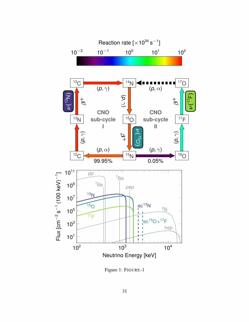
“metals” directly catalyse the CNO cycle, and ii) they affect the plasma opacity, indirectly chang-ing the temperature of the core and modifying the evolution of the Sun and its density profile. Wenotice that in the Sun the CNO sub-cycle I (see Fig. 1, upper plot) is dominant 4.

The CNO neutrino flux scales with the metal abundance in the solar core, itself a tracer ofthe initial chemical composition of the Sun at the time of its formation. The metal abundance inthe core is thought to be decoupled from the surface by a radiative zone, where no mixing occurs.CNO neutrinos are the only probe of that initial condition.

The neutrinos produced by the solar pp chain have been extensively studied since the early70’s leading the discovery of nuclear fusion reactions in the Sun and the matter-enhanced neutrinoflavour conversion 5–11. Recently, the Borexino experiment has published a comprehensive studyof the neutrino from the pp chain 12.

We report here the first direct detection of the CNO solar neutrinos and prove that the catal-ysed hydrogen fusion envisaged by Bethe and Weizsacker in the 30’s indeed exists 13, 14. This resultquantifies the rate of the CNO cycle in the Sun and paves the way to the solution of the long stand-ing “solar metallicity problem” 2 arising from the discrepancy on the metallicity predicted by solarmodels using updated (low) metal abundances from spectroscopy (SSM-LZ) 18 and that inferredfrom helioseismology, which favors a higher metal content (SSM-HZ). Despite detailed studies,this puzzle remains an open problem in solar physics.

The observation of CNO neutrinos reported here experimentally confirms the overall solarpicture and shows that a direct measurement of the metallicity of the Sun’s core is within reach ofan improved, future measurement.

Borexino detector and data

Borexino is a solar neutrino experiment located underground at the Laboratori Nazionali del GranSasso in Italy, where the cosmic muon flux is suppressed by a factor of ∼106. The detector ac-tive core consists of approximately 280 tonnes of liquid scintillator contained in a spherical nylonvessel of 4.25 m radius. Particles interacting in the scintillator emit light that is detected by 2212photomultiplier tubes 19 (PMTs).

Solar neutrinos are detected in Borexino via elastic scattering off electrons. The total number

2

of detected photons and their arrival times are used to reconstruct the electron recoil energy andthe interaction point in the detector, respectively. The energy and spatial resolution in Borexinohas slowly deteriorated over time due to the steady loss of PMTs (on average 1238 channels areactive for this analysis) and they are currently σE/E ≈6% and σx,y,z ≈11 cm for 1 MeV events atthe center of the detector.

The time profile of the scintillation light provides a powerful way to distinguish among dif-ferent particle types (α, β−, and β+) via pulse-shape discrimination methods 20, 21 and is essentialfor the selection of 210Po α decays used to constrain 210Bi background, as discussed below.

In spite of the very high number of solar neutrinos reaching the Earth (≈6× 1010 ν cm−2 s−1)their interaction rate is low, namely few tens of counts per day (cpd) in 100 tonnes (t) of scintillator.Their detection is especially challenging, because the neutrino signals cannot be easily disentan-gled from radioactive backgrounds. Borexino’s success rests on its unprecedented radio-puritycombined with the careful selection of materials 22 and clean assembly protocols.

This paper is based on data collected during Borexino Phase-III, from July 2016 to February2020, corresponding to 1072 days of live time. The event sample is filtered by applying a set ofselection criteria 21 that reduce events from residual radioactive impurities, cosmic muons, cosmo-genic isotopes, instrumental noise, and external gamma rays. The latter are significantly suppressedby selecting events occurring within an innermost volume of scintillator (fiducial volume, FV) de-fined by a cut on the reconstructed radius and vertical position (r < 2.8 m and -1.8 m<z < 2.2 m).Data are analysed in the electron recoil energy interval from 320 to 2640 keV.

The counting rate of events surviving the selection as a function of their visible energy isshown in Fig. 2. The data distribution is understood to be the sum of solar neutrino componentsand of backgrounds due to the decays of residual radioactive contaminants of the scintillator (85Kr,210Bi, 210Po, 40K) and of cosmogenic 11C, and to γ-rays from the decays of 40K, 214Bi, and 208Tl inthe materials external to the scintillator. These backgrounds have been characterized in Phase-II 21

and their rates range between a few and tens of cpd per 100 t , to be compared with the expectedCNO signal of a few cpd per 100 t . The key backgrounds for this study are 11C and 210Bi. Togetherwith solar pep neutrinos (an alternative proton fusion first step of the pp chain), they represent themain obstacle to the extraction of the CNO signal, as discussed in the next section. The expectedbackground due to the elastic scattering of 40K geo-antineutrinos 25 is negligible. The yellow ver-tical band in Fig. 2 highlights the region of largest CNO signal-to-background ratio.

3

CNO neutrino detection strategy and the 210Bi challenge

Neutrinos from the CNO cycle produce a broad energy spectrum ranging between 0 and 1740 keV(see Fig. 1, lower plot). Consequently, the recoil energy of electrons has a rather featureless con-tinuous distribution that extends up to 1517 keV (see Fig. 2). In this work, the three CNO neutrinocomponents (Fig. 1) were treated as a single contribution by fixing the ratio between them accord-ing to the SSM prediction 1, 2. Several backgrounds contribute to the same energy interval with arate comparable to or larger than the signal. To disentangle all contributions, we fit the data with aprocedure similar to that adopted in 12, 21, 26 and described in Methods.

The CNO analysis is affected by two additional complications: the similarity between theCNO-ν recoil electron and the 210Bi β− spectra and their strong correlations with the pep-ν recoilelectron spectrum. In addition, the data are contaminated by cosmogenic 11C in the high energypart of the CNO spectrum. The muon-neutron-positron three-fold-coincidence (TFC) tagging tech-nique 21 for 11C is essential to make the CNO detection possible.

The sensitivity to CNO neutrinos is low unless the 210Bi and pep-ν rates are sufficientlyconstrained in the fit 27. The pep-ν rate is constrained to 1.4% precision 27, using: solar luminosity,robust assumptions on the pp to pep neutrino rate ratio, existing solar neutrino data 28, 29, and themost recent oscillation parameters 30. We underline that the luminosity of the Sun depends veryweakly on the contribution of the CNO cycle, making the pep constraint essentially independent ofany reasonable assumption on the CNO rate.

The other main background for the CNO-ν measurement comes from the decays of 210Bi 27,a β emitter with a short half-life (5.013 days) and whose decay rate is supported by 210Pb throughthe sequence:

210Pbβ−

−−−−−→22.3 years

210Biβ−−−−→5 days

210Poα−−−−−→

138.4 days

206Pb . (1)

We note that the endpoint energy of the 210Pb β-decay is 63.5 keV, well below the analysis thresh-old (320 keV). Therefore, the determination of the 210Bi content must rely on measuring 210Po 31.The α particles from 210Po decay, selected event-by-event by means of pulse-shape discrimination,are ideal tracers of 210Bi , if secular equilibrium in sequence (1) is achieved. It is hence crucial tounderstand under what conditions such an equilibrium is established.

Since 2007, the data have shown that out-of-equilibrium components of 210Po were presentin the fiducial volume. A dedicated effort was implemented to study and ultimately to prevent

4

these components from migrating into the fiducial volume by stabilising the detector temperature.This upgrade allowed us to reach a sufficient equilibrium in one central sub-volume of the detector,which made the result reported in this paper possible. We distinguish between a Scintillator (S)210Po component (210PoS) sourced by 210Pb in the liquid and assumed to be stable in time andin equilibrium with 210Bi, and a Vessel (V) component (210PoV). The source of 210PoV for thisdataset is understood to be 210Pb deposited on the inner surfaces of the vessel. The daughter 210Pomay detach and move into the scintillator by diffusion or following slow convective currents. It isimportant to note that, as explained in detail below, there is no evidence of 210Pb itself leachingfrom those surfaces, since the rate of 210Bi observed in the scintillator has not significantly changedover several years.

The diffusion length of 210Po atoms in one half-life is significantly less than the separationbetween the vessel and the FV (approximately 1 m). We can therefore conclude that diffusion isnegligible for both 210Po and 210Bi . However, Borexino data show that slow convective currentscaused by temperature gradients and variations may indeed carry the 210Po into the FV. The sameeffect does not occur for the short-lived 210Bi that might also detach from the vessel, since it decaysbefore reaching the FV.

Prior to 2016, Borexino was equipped with neither detailed temperature mapping, thermalinsulation, or active temperature control. Convective currents were substantial, because of seasonaltemperature variations and human activities affecting the temperature of the experimental hall. Thelarge fluctuations of the 210Po activity in the FV induced by these currents are shown in Fig. 3,where the 210Po rate in different detector positions is plotted as a function of time. It is evidentthat before 2016 the 210Po counts in the FV were both high (> 100 cpd per 100 t) and greatlyunstable, on time scales shorter than the 210Po half-life, because of sizeable fluid movements,which prevented the separation of PoS from PoV.

In order to suppress convection, a stable vertical thermal gradient needed to be established.The Borexino installation atop a cold floor in contact with the rock, acting as an infinite thermalsink, offers a unique opportunity to achieve such a gradient, once the detector is insulated againstinstabilities of the air temperature. Thermal insulation of the detector was completed in December2015 and an active temperature control system 33 was installed in January 2016 atop the detector(see Methods). A residual seasonal modulation of the order of 0.3◦C/6 months is still visible in thedetector and in the rock below it, but its effect is small for the purpose of this paper.

5

This extensive stabilisation effort paid off: the 210Po rate initially decreased and reached itslowest value in a region that we named Low Polonium Field (LPoF), above the equator aroundz ' +80 cm. The existence of this volume, compatible in size and location with fluid dynamicssimulation 34, is crucial in determining the 210Bi constraint. We note that the result of this paper isstable against small variations of the shape and location of the LPoF.

210Bi constraint

The amount of 210Bi in the scintillator is determined from the minimum value of the 210Po rate inthe LPoF through the relation

R(210Pomin) = R(210Bi) + R(210PoV), (2)

where, as discussed above, the 210Bi rate is equal to 210PoS according to secular equilibrium. Since210PoV is always positive, 210Pomin yields an upper limit for the 210Bi rate.

The 210Po content is not spatially uniform within the LPoF but exhibits a clear minimumwith no sizable plateau around it. This yields a robust upper limit for the rate of 210Bi, but doesnot guarantee that 210PoV is actually zero. Only a spatially extended minimum of the 210Po ratewould have yielded a measurement of the 210Bi rate.

The minimum 210Po rate was estimated from the 210Po distribution within the LPoF with 2Dand 3D fits following two mutually compatible procedures (see Methods). The spatial position ofthe minimum is stable over the analysis period (it slowly moves by less than 20 cm per month),showing that the detector is in a fluid dynamical quasi-steady condition and that the 210Po rateminimum is not a statistical fluctuation. Both procedures consistently yieldR(210Pomin) = (11.5±1.0) cpd per 100 t. The error includes the systematic uncertainty of the fit (see Methods).

The 210Bi rate can then be extrapolated over the whole FV, provided that it is uniform inthe FV during the time period over which the estimation is performed. Lacking the possibility toindividually tag 210Bi events, the analysis is performed by selecting β-like events at energies wherethe relative bismuth contribution is maximum. We find the 210Bi angular and spatial distributionuniform within errors. The systematic uncertainty associated to possible spatial non-uniformity of210Bi is conservatively estimated at 0.78 cpd per 100 t. The observed 210Bi uniformity in Phase-IIIis expected from the substantial fluid mixing that has occurred prior to the thermal insulation, andagrees with 2D and 3D fluid dynamic simulations.

6

Because of the low velocity of convection currents, the uniformity of 210Bi provides a con-vincing evidence that 210Pb does not leach off the vessel. As a cross check, the rate of β-like eventsshows the expected 3.3% annual modulation of the solar neutrino rate (dominated by 7Be-ν) dueto the eccentricity of the Earth’s orbit, proving that background β-like events are stable in time.See Methods for details.

In summary, the 210Bi rate used as a constraint in the CNO-ν analysis is:

R(210Bi) ≤ (11.5± 1.3) cpd per 100 t, (3)

which includes the statistical and systematic uncertainties in the 210Po minimum determinationand the systematic uncertainty related to the 210Bi uniformity hypothesis (added in quadrature).

Results and conclusions

We performed a multivariate analysis, simultaneously fitting the energy spectra in the window be-tween 320 keV and 2640 keV and the radial distribution of the selected events, with details givenin Methods. The following rates are treated as free parameters: CNO neutrinos, 85Kr, 11C, internaland external 40K, external 208Tl and 214Bi, and 7Be neutrinos. The pep neutrino rate is constrainedto (2.74 ± 0.04) cpd per 100 t by multiplying the standard likelihood with a symmetric Gaussianterm. The upper limit to the 210Bi rate obtained from eq. 3 is enforced asymmetrically by multi-plying the likelihood with a half-Gaussian term, i.e., leaving the 210Bi rate unconstrained between0 and 11.5 cpd per 100 t .

The reference spectral and radial distributions (PDFs) of each signal and background speciesto be used in the multivariate fit are obtained with a complete GEANT4-based Monte Carlo sim-ulation 21, 36. The results of the multivariate fit for data in which the 11C has been subtracted withthe TFC technique are shown in Fig. 2. The p-value of the fit is high (0.3) demonstrating the goodagreement between data and the underlying fit model. The corresponding negative log-likelihoodfor CNO-ν, profiled over the other neutrino fluxes and background sources, is shown in Fig. 4(dashed black line in the right panel). The best fit value is 7.2 cpd per 100 t with an asymmetricconfidence interval of -1.7 cpd per 100 t and +2.9 cpd per 100 t (68% C.L., statistical error only),obtained from the quantile of the likelihood profile.

We have studied possible sources of systematic error following an approach similar to theone used in 12, 21. We have investigated the impact of varying fit parameters (fit range and binning)

7

on the result by performing 2500 fits in different conditions and found it to be negligible with re-spect to the CNO statistical uncertainty. We also considered the effect of different theoretical 210Bishapes from 37–39 and found that the CNO result is robust with respect to the selected one 37. Dif-ferences are included in the systematic error. We have performed a detailed study of the impact ofpossible deviations of the energy scale and resolution from the Monte Carlo model: non-linearity,non-uniformity, and variation in the absolute magnitude of the scintillator light yield have beeninvestigated by simulating several million Monte Carlo pseudo-experiments with deformed shapesand fitting them with the regular non-deformed PDFs. The magnitude of the deformations waschosen to be within the range allowed by the available calibrations 40 and by two ”standard can-dles” (210Po, 11C) present in the data. The overall contribution to the total error of all these sourcesis -0.5/+0.6 cpd per 100 t. Folding the systematic uncertainty over the log-likelihood profile wedetermine the final CNO interaction rate to be 7.2 +3.0

−1.7 cpd per 100 t. The rate can be converted toa flux of CNO-ν on Earth of 7.0 +3.0

−2.0 × 108 cm−2 s−1, assuming MSW conversion in matter 41, neu-trino oscillation parameters from 42 and Refs. therein, and a density of electrons in the scintillatorof (3.307± 0.015)× 1031 e− per 100 t.

Other sources of systematic error investigated in the previous precision measurement of thepp chain 12, such as, fiducial volume, scintillator density, and lifetime were found to be negligiblewith respect to the large CNO statistical uncertainty.

The log-likelihood profile including all the errors combined in quadrature is shown in Fig. 4right (black solid line). The asymmetry of the profile is due to the applied half-Gaussian constrainton the 210Bi , see eq. (3) and causes the profile to be relatively steep on the left side of the minimum.The shallow shape on the right side of the profile reflects the modest sensitivity to distinguish thespectral shapes of 210Bi and CNO recoil spectra. From the corresponding profile-likelihood we ob-tain a 5.1σ significance of the CNO observation. Additionally, a hypothesis test based on a profilelikelihood test statistic 43 using 13.8 million pseudo-data sets with the same exposure of Phase-IIIand systematic uncertainties included (see Methods) excludes the no-CNO signal scenario with asignificance better than 5.0σ at 99.0% C.L.

This observed CNO rate is compatible with both SSM-HZ and SSM-LZ predictions. Thuswe cannot distinguish between the two different models (we quote the statistical compatibility forthe reader: HZ is at 0.5σ and LZ is at 1.3σ), see Fig. 4. When combined with other solar neutrinofluxes measured by Borexino the LZ hypothesis is disfavoured at 2.1σ.

8

We underline that the sensitivity to CNO neutrinos mainly comes from a small energy regionbetween 780 keV and 885 keV (region of interest, ROI, see yellow band in Fig. 2), where the signal-to-background ratio is maximal 27. In this region, the count rate is dominated by events from CNOand pep neutrinos, and by 210Bi decays. The remaining backgrounds contribute less than 20%(see Fig. 4, left plot). A simple counting analysis confirms that the number of events in the ROIexceeds the sum from all known backgrounds, leaving room for CNO neutrinos, as depicted inFig. 4, left. In this simplified approach (described in detail in Methods), we use the 210Bi rate asdetermined in eq. 3 applying a symmetric Gaussian penalty and assuming an analytical descriptionof the background model and the detector response. The statistical significance of the presence inthe data of CNO neutrino events from this counting analysis, after accounting for statistical andsystematic errors is lower (' 3.5σ) than that obtained with the main analysis, given the simplifiednature of this approach. In conclusion, we exclude the absence of a CNO solar neutrino signal witha significance of 5.0σ. This is the first direct detection of CNO solar neutrinos.

Acknowledgements We acknowledge the generous hospitality and support of the Laboratori Nazionalidel Gran Sasso (Italy). The Borexino program is made possible by funding from Istituto Nazionale di FisicaNucleare (INFN) (Italy), National Science Foundation (NSF) (USA), Deutsche Forschungsgemeinschaft(DFG) and Helmholtz-Gemeinschaft (HGF) (Germany), Russian Foundation for Basic Research (RFBR)(Grants No. 16-29-13014ofi-m, No. 17-02-00305A, and No. 19-02-00097A) and Russian Science Foun-dation (RSF) (Grant No. 17-12-01009) (Russia), and Narodowe Centrum Nauki (NCN) (Grant No. UMO2017/26/M/ST2/00915) (Poland). We gratefully acknowledge the computing services of Bologna INFN-CNAF data centre and U-Lite Computing Center and Network Service at LNGS (Italy), and the computingtime granted through JARA on the supercomputer JURECA 44 at Forschungszentrum Julich (Germany).This research was supported in part by PLGrid Infrastructure (Poland).

Authors Contributions The Borexino detector was designed, constructed, and commissioned by the Borex-ino Collaboration over the span of more than 30 years. The Borexino Collaboration sets the science goals.Scintillator purification and handling, material radiopurity assay, source calibration campaigns, photomul-tiplier tube and electronics operations, signal processing and data acquisition, Monte Carlo simulations ofthe detector, and data analyses were performed by Borexino members, who also discussed and approved thescientific results. This manuscript was prepared by a subgroup of authors appointed by the Collaborationand subjected to an internal collaboration-wide review process. All authors reviewed and approved the finalversion of the manuscript.

Competing Interests The authors declare that they have no competing financial interests.

Correspondence Correspondence and requests for materials should be addressed to the Borexino Collab-

9

oration through the spokesperson’s email: spokesperson-borex@lngs.infn.it.

Data Availability The datasets generated during the current study are freely available in the repositoryhttps://bxopen.lngs.infn.it/. Additional information is available from the Borexino Collaboration spokesper-son (spokesperson-borex@lngs.infn.it) upon reasonable request.

The Borexino Collaboration*

M. Agostini1, 2, K. Altenmuller2, S. Appel2, V. Atroshchenko3, Z. Bagdasarian4,26, D. Basilico5,G. Bellini5, J. Benziger6, R. Biondi7, D. Bravo5,27, B. Caccianiga5, F. Calaprice8, A. Caminata9,P. Cavalcante10,28, A. Chepurnov11, D. D’Angelo5, S. Davini9, A. Derbin12, A. Di Giacinto7, V. DiMarcello7, X.F. Ding8, A. Di Ludovico8, L. Di Noto9, I. Drachnev12, A. Formozov13,5, D. Franco14,C. Galbiati8,15, C. Ghiano7, M. Giammarchi5, A. Goretti8,28, A.S. Gottel4,16, M. Gromov11,13,D. Guffanti17, Aldo Ianni7, Andrea Ianni8, A. Jany18, D. Jeschke2, V. Kobychev19, G. Korga20,30,S. Kumaran4,16, M. Laubenstein7, E. Litvinovich3,21, P. Lombardi5, I. Lomskaya12, L. Ludhova4,16,G. Lukyanchenko3, L. Lukyanchenko3, I. Machulin3,21, J. Martyn17, E. Meroni5, M. Meyer22,L. Miramonti5, M. Misiaszek18, V. Muratova12, B. Neumair2, M. Nieslony17, R. Nugmanov3,21

L. Oberauer2, V. Orekhov17, F. Ortica23, M. Pallavicini9, L. Papp2, L. Pelicci5, O. Penek4,16,L. Pietrofaccia8, N. Pilipenko12, A. Pocar24, G. Raikov3, M.T. Ranalli7, G. Ranucci5, A. Razeto7,A. Re5, M. Redchuk4,16, A. Romani23, N. Rossi7, S. Schonert2, D. Semenov12, G. Settanta4,M. Skorokhvatov3,21, A. Singhal4,16, O. Smirnov13, A. Sotnikov13, Y. Suvorov7,3,29, R. Tartaglia7,G. Testera9, J. Thurn22, E. Unzhakov12, F.L. Villante7,25, A. Vishneva13, R.B. Vogelaar10, F. von Feilitzsch2,M. Wojcik18, M. Wurm17, S. Zavatarelli9, K. Zuber22, G. Zuzel18.

*Corresponding address: spokesperson-borex@lngs.infn.it

1Department of Physics and Astronomy, University College London, Gower Street, London WC1E6BT, UK;2Physik-Department E15, Technische Universitat Munchen, 85748 Garching, Germany;3National Research Centre Kurchatov Institute, 123182 Moscow, Russia;4Institut fur Kernphysik, Forschungszentrum Julich, 52425 Julich, Germany;5Dipartimento di Fisica, Universita degli Studi and INFN, 20133 Milano, Italy;6Chemical Engineering Department, Princeton University, Princeton, NJ 08544, USA;7INFN Laboratori Nazionali del Gran Sasso, 67010 Assergi (AQ), Italy;8Physics Department, Princeton University, Princeton, NJ 08544, USA;

10

9Dipartimento di Fisica, Universita degli Studi and INFN, 16146 Genova, Italy;10Physics Department, Virginia Polytechnic Institute and State University, Blacksburg, VA 24061,USA;11Lomonosov Moscow State University Skobeltsyn Institute of Nuclear Physics, 119234 Moscow,Russia;12St. Petersburg Nuclear Physics Institute NRC Kurchatov Institute, 188350 Gatchina, Russia;13Joint Institute for Nuclear Research, 141980 Dubna, Russia;14Universite de Paris, CNRS, Astroparticule et Cosmologie, F-75013 Paris, France;15Gran Sasso Science Institute, 67100 L’Aquila, Italy;16III. Physikalisches Institut B, RWTH Aachen University, 52062 Aachen, Germany;17Institute of Physics and Excellence Cluster PRISMA+, Johannes Gutenberg-Universitat Mainz,55099 Mainz, Germany;18M. Smoluchowski Institute of Physics, Jagiellonian University, 30348 Krakow, Poland;19Institute for Nuclear Research of NAS Ukraine, 03028 Kyiv, Ukraine;20Department of Physics, Royal Holloway, University of London, Department of Physics, Schoolof Engineering, Physical and Mathematical Sciences, Egham, Surrey, TW20 OEX;21National Research Nuclear University MEPhI (Moscow Engineering Physics Institute), 115409Moscow, Russia;22Department of Physics, Technische Universitat Dresden, 01062 Dresden, Germany;23Dipartimento di Chimica, Biologia e Biotecnologie, Universita degli Studi e INFN, 06123 Peru-gia, Italy;24Amherst Center for Fundamental Interactions and Physics Department, University of Mas-sachusetts, Amherst, MA 01003, USA;25Dipartimento di Scienze Fisiche e Chimiche, Universita dell’Aquila, 67100 L’Aquila, Italy.26Present address: University of California, Berkeley, Department of Physics, CA 94720, Berkeley,USA;27Present address: Departamento de Fısica Teorica, Universidad Autonoma de Madrid, CampusUniversitario de Cantoblanco, 28049 Madrid, Spain;28Present address: INFN Laboratori Nazionali del Gran Sasso, 67010 Assergi (AQ), Italy;29Present address: Dipartimento di Fisica, Universita degli Studi Federico II e INFN, 80126Napoli, Italy;30Also at Institute of Nuclear Research (Atomki), H-4001, Debrecen, POB.51., Hungary.

11

Methods

Experimental setup and neutrino detection technique

The Borexino detector 19 was designed and built to achieve the utmost radio-purity at its core. It ismade of an unsegmented Stainless Steel Sphere (SSS) mounted within a large Water Tank (WT).The SSS contains the organic liquid and supports the photomultipliers (PMTs), while the watershields the SSS against external radiation and is the active medium of a Cherenkov muon tagger.A schematic drawing is shown in ED Fig. 1.

Within this SSS, two thin (125µm) nylon vessels separate the volume in three shells of radii4.25 m, 5.50 m, and 6.85 m, the latter being the radius of the SSS itself.

The inner nylon vessel (IV), concentric to the SSS, contains a solution of Pseudocumene(PC) as solvent and PPO (2,5-diphenyloxazole) as fluor dissolved at a concentration of about1.5 g/l. The second and the third shells are filled with a buffer liquid comprised of a solutionof DMP (dimethylphthalate) in PC. The purpose of this double buffer is to shield the IV against γradiation emitted by contaminants present in the PMTs and the steel, while the outer nylon vesselprevents the diffusion of emanated Radon into the IV. The total amount of liquid within the SSS isapproximately 1300 tonnes, of which about 280 tonnes are the active liquid scintillator.

The IV scintillator density is slightly smaller than that of the buffer liquid, yielding an upwardbuoyant force. The IV is therefore anchored to the bottom of the SSS through thin high molecularweight polyethylene cords, thus minimising the amount of material close to the scintillator andkeeping the IV in stable mechanical equilibrium.

The SSS is equipped with nominally 2212 8” PMTs that collect scintillation light emit-ted when a charged particle, either produced by neutrino interactions or by radioactivity, releasesenergy in the scintillator. Most of the PMTs (1800) are equipped with light concentrators (Win-ston cones) for an effective optical coverage of 30%. Scintillation light is detected at approx-imately 500 photoelectrons per MeV of electron equivalent of deposited energy (normalized to2000 PMTs). In organic liquid scintillators, the light yield per unit of deposited energy is affectedby ionisation quenching 45. Alpha particles, characterised by higher ionisation rates along theirpath, experience more quenching compared to electrons and thus, produce less scintillation light.The distribution of photon arrival times on PMTs allows the reconstruction of the location of theenergy deposit by means of time-of-flight triangulation and the determination of the particle typeby exploiting the pulse shape 21.

12

The very nature of the scintillation emission makes it impossible to distinguish the signalemitted by electrons scattered by neutrinos from that produced by electrons emitted in nuclear βdecays or Compton-scattered by γ rays. Therefore, the radioactive background must be kept ator below the level of the expected signal rate, which for the total solar neutrino spectrum is of theorder of a few events per tonne per day and, in the case of CNO neutrinos, two orders of magnitudesmaller. Taking into account that typical materials (air, water, metals) are normally contaminatedwith radioactive impurities at the level of 10,000 or even 100,000 decays per tonne per second, thisrequirement is indeed a formidable challenge.

The scintillator procurement procedure was conceived to select an organic hydrocarbon witha very low 14C(β−, Q= 156 keV) content. Carbon-14 is cosmogenically activated in atmosphericcarbon and an irreducible radioactive contaminant in organic hydrocarbons. The scintillator wasdelivered to the Gran Sasso laboratory in special tanks following procedures conceived to avoidcontamination and to minimise the exposure to cosmic rays, which also produce other long livingisotopes. Once underground, it was purified following various steps in plants specifically devel-oped over more than 10 years for this purpose and installed close to the detector. The purificationduring the 2007 initial scintillator fill was done mainly by distillation and counterflow spargingusing low-argon-krypton nitrogen. A dedicated purification campaign in 2010 - 2011 processedthe scintillator through several cycles of ultra-pure water extraction. These purification techniquesare described in 46, 47, and 21.

This effort paid off: the extreme purity of the scintillator and the careful selection of thematerial surrounding it (nylon, plastic supports of the nylon vessels, steel, and PMT glass in partic-ular), the use of carefully selected components (valves, pumps, fittings, etc.) together with specialcare during detector construction and installation yielded unprecedented low values of radioactivecontaminants in the active scintillator. In addition, through the selection of a fiducial volume, theresidual external gamma ray background (from IV nylon, SSS, and PMTs) is substantially reducedfurther. All Borexino results owe directly to this unprecedented radio-purity.

The Water Tank is itself equipped with 208 PMTs to detect Cherenkov light emitted bymuons crossing the water. The capability to detect muons, to reconstruct their tracks throughthe scintillator was crucial to identify and tag cosmogenic contaminants (i.e. short living nucleiproduced by muon spallation with scintillator components 48, 49), especially 11C background. Muontagging allows Borexino to also efficiently detect cosmogenic neutrons 50, which occasionally areproduced with high multiplicity, another crucial ingredient in 11C tagging.

13

Thermal insulation system and control

The thermal stability of the Borexino detector is required to avoid undesired background variationsdue to the mixing of the scintillator inside the Inner Vessel. This mixing is caused by convectivecurrents induced by temperature changes due to human activities in the underground Hall and toseasonal effects. A significant upgrade of the detector in this respect was carried out.

Between May and December 2015, 900 m2 of thermal insulation was installed on the outsideof the Borexino Water Tank. In addition, the system used to recirculate water inside the WT wasstopped in July 2015 to contribute to the inner detector thermal stability and allow its fluid tovertically stratify.

The thermal insulation consists of two layers: an outer 10 cm layer of Ultimate Tech Roll 2.0mineral wool (thermal conductivity at 10◦C of 0.033 W/m/K) and an inner 10 cm layer of UltimateProtect wired Mat 4.0 mineral wool reinforced with Al foil 65 g/cm2 with glass grid on one side(thermal conductivity at 10◦C of 0.030 W/mK). The thermal insulation material is anchored to theWT with 20 m long nails on a metal plate attached to the tank (5 nails/m2). In addition, an activetemperature control system (ATCS) was completed in January 2016. In ED Fig. 2 the BorexinoWT is shown wrapped in thermal insulation.

A system of 66 probes with 0.07◦C resolution, the position of which is shown in ED Fig. 3,monitors the temperature of Borexino. They are arranged as follows: 14 protruding 0.5 m radiallyinward into the SSS (ReB probes) and in operation since October 2014, measure the temperatureof the outer part of the buffer liquid (OB); 14 mounted 0.5 m radially outward from the SSS (ReWprobes) and in operation since April 2015, measure the temperature of the water; 20 installedbetween the insulation layer and the external surface of the WT (WT probes) are in operationsince May 2015; 4 located inside a pit underneath the Borexino WT are in operation since October2015; 14 on the Borexino detector WT dome installed in early 2016. Since 2016 the averagetemperature of the floor underneath the detector in contact with the rock is 7.5◦C, while at the topof the detector it is 15.8◦C. This temperature difference corresponds to a naturally-driven gradient∆T/∆z > 0 ∼ 0.5◦C/m. Ensuring this gradient does not decrease it is the key to reducingconvective currents, scintillator mixing, and consequently stabilizing the 210Po background for theCNO analysis.

Out of the last 14 probes, three are part of the Active Temperature Control System (ATCS)kept in operation during the present data taking. The ATCS consists of a water based system madewith copper tube coils installed on the upper part of the detector’s dome. The coils are in contact

14

with the WT steel, with the addition of an Al layer to enhance the thermal coupling. A 3 kWelectric heater, a circulation pump, a temperature controller, and an expansion tank are connectedto the coils. The ATCS trims the natural thermal gradient and is essential to eliminate convectionmotion.

The Outer Detector head tank (a 70-liter vessel connected with the 1346 m3 volume of theSSS) is used as a sensitive detector thermometer. After the thermal insulation system installationthe head tank had to be refilled with 289 kg of PC because of the detector overall cooling andcorresponding shrinkage. Calibration established the sensitivity of this thermometer to be of theorder of 10−2 ◦C per 100 mm change of fluid height.

The deployment of both the thermal insulation and the temperature control systems werequickly effective in stabilizing the inner detector temperature. As of 2016 the heat loss due to thethermal insulation system was equal to 247 W. Yet, changes of the experimental hall temperatureinduced residuals variations in the top buffer probes of the order of 0.3◦C/6 months. To furtherreduce these effects an active system to control the seasonal changes of the air temperature enter-ing the experimental Hall and surrounding the Borexino WT was designed and installed in 2019.It consists of a 70 kW electrical heater installed inside the inlet air duct, which has a capacity12000 m3/h (in normal conditions). The heater is deployed just a few meters before the Hall maindoor. The temperature control is based on a master/slave architecture with a master PID controllerthat acts on a second slave PID controller. Probes deployed around the WT monitor the temper-ature of the air. After commissioning, a set point temperature for the master PID of 14.5◦C ischosen. This system controls the temperature of the inlet air within approximately 0.05◦C.

The thermal insulation, active temperature control of the detector, and the Hall C air temper-ature control have enabled remarkable temperature stability of the detector. ED Figure 4 shows thetemperature time profile read by all probes since 2016. A stable temperature gradient was clearlyestablished as needed to avoid mixing of the scintillator.

The Low Polonium Field and its properties

After the completion of the thermal insulation (Phase-III), the Bismuth-210 background activity ismeasured from the 210Po activity assuming secular equilibrium of the A = 210 chain. The mea-sured 210Po rate is the sum of two contributions: a scintillator 210Po component supported by the210Pb in the liquid (210PoS), which we assume to be stable in time and equal to the intrinsic rateof 210Bi in the scintillator, and a vessel component (210PoV). The latter has a 3D diffusive-likestructure given by polonium detaching from the Inner Vessel and migrating into the fiducial vol-

15

ume. The origin of this component is the 210Pb contamination of the vessel. The 210Po migrationprocess is driven by residual convective currents. A rough estimation of the migration length λmig

obtained by fitting the spatial distribution of 210Po, is found to range between 50 and 100 cm, whichcorresponds to a migration coefficient Dmig = (1.0 ± 0.4) × 10−9 m2 s−1 (where we have usedthe relation λmig =

√DmigτPo with the 210Po lifetime, τPo = 199.7 days). This value is slightly

lower than the diffusion coefficient Ddiff ∼ 1.5× 10−9 m2 s−1 (corresponding to a diffusion lengthλdiff ∼ 20 cm), predicted by the Stokes-Einstein formula 51 and observed for heavy atoms in hy-drocarbons 32. We interpret this difference as due to the presence of residual convective motionsin Phase-III. These motions are localized in small regions and create a diffusive-like structure withan effective migration length λmig & λdiff .

The α’s from 210Po decays are selected event-by-event with a highly efficient α/β pulseshape discrimination neural network method based on a Multi-layer Perceptron (MLP) 52. Theresulting three-dimensional 210Po activity distribution, named the Low Polonium Field (LPoF),exhibits an effective migration profile with an almost stable minimum located above the detectorequator (see 3D shape in ED Fig. 5, and dark blue regions in ED Fig. 6 top). The qualitative shapeand approximate position of the LPoF is reproduced by fluid dynamical numerical simulationsreported in 34.

Assuming azimuthal symmetry around the detector z-axis, confirmed by 3D analysis, the210Po minimum activity is determined by fitting LPoF with a 2D paraboloidal function:

d2R(210Po)

d(ρ2)dz=[R(210Pomin)εEεMLP +Rβ

]×

×(

1 +ρ2

a2+

(z − z0)2

b2

),

(4)

where ρ2 = x2 + y2, a and b are the paraboloid axes, z0 is the position of the minimum along the zaxis, εE and εMLP are the efficiency of energy and MLP cuts used to select α’s from 210Po decays,and Rβ is the residual rate of β events after the selection of α’s. The fit is initially performed indata bins of 2 months, but compatible results are obtained using the bins of 1 month. ED Figure 6top shows the result of the z0 minimum position as a function of time. The minimum slowly movesalong the z direction by less than 20 cm per month. In order to perform a better estimation of the210Po minimum, we sum up all the time bins after aligning the 3D distributions with respect to z0.Possible intrinsic biases, due to the minimum determination in different time intervals, have beenminimized by blindly aligning the data from each time bin according to the z0 inferred from theprevious time interval.

16

The distribution of 210Po events after applying this procedure is shown in ED Fig. 6 bottom,where the LPoF structure is clearly visible. The final fit is then performed on 20 tonnes of thisaligned data set containing about 5000 210Po events. From this fit we extract the 210Po minimum.This value might still have a small contribution from the vessel component (eq. 2), i.e. R(210Bi) ≤R(210Pomin). Therefore this method provides only an upper limit for the 210Bi rate. A companionanalysis was performed using a 3D paraboloidal function. The 2D and 3D fits were performed witha standard binned likelihood and a Bayesian approach using non-informative priors. In particular,the latter was implemented with MULTINEST 53–55, a nested sampling algorithm.

In addition, because the shape of the LPoF might show more complexity along the z-axisthan a simple paraboloidal shape, a Bayesian framework was also used to perform the fit with acubic spline along the z axis. Splines are piecewise polynomials connected by knots. The numberof knots defines the complexity of the curve. To prevent over-fitting, a Bayesian factor analysis wasused to decide on the most appropriate number of knots for the data set. While it was found that thesplines were, in general, a better fit to the data (Bayes factor > 102), the final result is compatibleto the simpler model within statistical uncertainties. This result has been further cross-checked byfitting the 210Po distribution along different angular directions with a family of analytical functionsfound as solution of the Fick diffusion equation 56 for the migration of decaying 210Po . Possiblebiases have been quantified by testing the fit model on simulated LPoF patterns based on numericalfluid dynamical simulations. They were found to be negligible for our purpose.

Spatial uniformity and time stability of 210Bi

The 210Bi independent constraint inferred from the LPoF can be extended over the whole fiducialvolume if, and only if, the 210Bi itself is uniform in space. Observation of the time stability of210Bi rate, not strictly required if the time periods of the LPoF and main analyses are the same, canadditionally crosscheck the overall robustness of the data set.

We have evidence that at the beginning of Borexino Phase-II, after the purification campaignperformed from 2010 to mid-2011, the 210Bi was not uniform: the cleanest part of the scintillatorwas concentrated on the top, partially out of the fiducial volume. In fact, the purification wasperformed in loop, taking the scintillator out from the bottom, purifying it, and re-inserting itfrom the top. For this reason, at the beginning of Phase-II the apparent 210Bi rate was higher andslowly decreased in time as mixing was taking place, thanks to the strong pre-insulation convectivecurrents. This decreasing trend stopped in early 2016 suggesting that the mixing had completed.Numerical fluid dynamical simulations, performed using as input the velocity field obtained from

17

210Po movements during the pre-insulation time, confirm this hypothesis.

A more conservative approach, which uses heuristic arguments based on the effective migra-tion of ions as measured from LPoF, suggests that 210Bi at the beginning of Phase-III (mid-2016)must be uniform at least within a volume scale of about 20 m3. This argument is also verified bymeans of fluid dynamics numerical simulations.

All the a priori arguments and qualitative studies described above are confirmed a posterioriby looking at the β event rate in optimized energy windows where the 210Bi signal-to-backgroundratio is maximal. The observed non-uniformity is then conservatively assigned only to 210Bi ,contributing about 15% to the overall rate in the selected energy window.

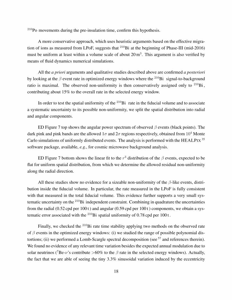
In order to test the spatial uniformity of the 210Bi rate in the fiducial volume and to associatea systematic uncertainty to its possible non-uniformity, we split the spatial distribution into radialand angular components.

ED Figure 7 top shows the angular power spectrum of observed β events (black points). Thedark pink and pink bands are the allowed 1σ and 2σ regions respectively, obtained from 104 MonteCarlo simulations of uniformly distributed events. The analysis is performed with the HEALPIX 35

software package, available, e.g., for cosmic microwave background analysis.

ED Figure 7 bottom shows the linear fit to the r3 distribution of the β events, expected to beflat for uniform spatial distribution, from which we determine the allowed residual non-uniformityalong the radial direction.

All these studies show no evidence for a sizeable non-uniformity of the β-like events, distri-bution inside the fiducial volume. In particular, the rate measured in the LPoF is fully consistentwith that measured in the total fiducial volume. This evidence further supports a very small sys-tematic uncertainty on the 210Bi independent constraint. Combining in quadrature the uncertaintiesfrom the radial (0.52 cpd per 100 t ) and angular (0.59 cpd per 100 t ) components, we obtain a sys-tematic error associated with the 210Bi spatial uniformity of 0.78 cpd per 100 t .

Finally, we checked the 210Bi rate time stability applying two methods on the observed rateof β events in the optimized energy windows: (i) we studied the range of possible polynomial dis-tortions; (ii) we performed a Lomb-Scargle spectral decomposition (see 57 and references therein).We found no evidence of any relevant time variation besides the expected annual modulation due tosolar neutrinos (7Be-ν’s contribute >60% to the β rate in the selected energy windows). Actually,the fact that we are able of seeing the tiny 3.3% sinusoidal variation induced by the eccentricity

18

of the Earth’s orbit around the Sun, is in itself a further proof of the excellent time stability of the210Bi rate. In particular, by studying the time dependence of the β-like events in the optimizedwindow, the uncertainty on the 210Bi rate change is 0.18 cpd per 100 t , which is indeed negligibleas compared with the global error quoted in Eq. 3.

We note that, even after complete mixing, the true 210Bi rate is not perfectly constant in time,as it must follow the decay rate of the parent 210Pb (τ = 32.7 y). This effect is not detectable overthe ∼3 years time period of our analysis, but for substantially longer periods it could be used forbetter constraining the 210Bi by fitting its long-lived temporal trend.

Details of the CNO analysis

The analysis presented in this work is based on the data collected from June 2016 to February2020 (Borexino Phase-III) and is performed in a fiducial volume (FV) defined as r < 2.8 m and−1.8 m<z < 2.2 m (r and z being the reconstructed radial and vertical position, respectively). Thetotal exposure of this dataset corresponds to 1072 days × 71.3 tonnes.

In Borexino, the energy of each event is given by the number of collected photoelectrons,while its position is determined by the photon arrival times at the PMTs. The energy and spatial res-olution in Borexino has slowly deteriorated over time due to the steady loss of PMTs (the averagenumber of active channels in Phase-III is 1238) and it is currently σE/E ≈6% and σx,y,z ≈11 cmfor 1 MeV events in the center of the detector.

Events are selected by a sequence of cuts, which are specifically designed to veto muonsand cosmogenic isotopes, to remove 214Bi - 214Po fast coincidence events from the 238U chain,electronic noise, and external background events. The fraction of neutrino events lost by thisselection criteria is measured with calibration data to be of the order of 0.1% and is thereforenegligible. More details on data selection can be found in 21.

The main backgrounds surviving the cuts and affecting the CNO analysis are: 210Bi and210Po in secular equilibrium with 210Pb which, as discussed thoroughly in the previous paragraphs,have a rate in Borexino Phase-III of ≤ (11.5± 1.3) cpd per 100 t ; 210PoV from the vessel; 85Kr (β,Q-value = 687 keV); 40K (β and γ, Q-value = 1460 keV), 11C (β+, Q-value = 960 keV; τ = 30 min),which is continuously produced by cosmic muons crossing the scintillator; γ rays emitted by 214Bi,208Tl, and 40K from materials external to the scintillator (buffer liquid, PMTs, stainless steel sphere,etc.).

19

CNO neutrinos are disentangled from residual backgrounds through a multivariate analy-sis, which includes the energy and radial distributions of the events surviving the selection. Dataare split into two complementary data sets: the TFC-subtracted spectrum, where 11C is selec-tively filtered out using the muon-neutron-positron three-fold coincidence algorithm (TFC) 20, 58

and the TFC-tagged spectrum, enriched in 11C. The TFC is a space and time coincidence veto-ing the 11C β+ decay events, by tagging the spallation muon and the neutron capture from thereactions: µ +12 C →11 C + n and n + p → d + γ. The reference shapes, i.e. the probabilitydistribution functions (PDFs) for signal and backgrounds used in the fit, are obtained through acomplete GEANT4-based Monte Carlo code 36, which simulates all physics processes occurring inthe scintillator, including energy deposition, photon emission, propagation, and detection, gener-ation and processing of the electronic signal. The simulation takes into account the evolution intime of the detector response and produces data that are reconstructed and selected following thesame pipeline of real data. The relevant input parameters of the simulation, mainly related to theoptical properties of the scintillator and of the surrounding materials, have been initially obtainedthrough small-scale laboratory tests and subsequently fine-tuned on calibration data, reaching anagreement at the sub-percent level 40. Data is then fitted as the sum of signal and background PDFs:the weights of this sum (the energy integral of the rates with zero threshold of each component inBorexino) are the only free parameters of the fit. The details of the multivariate fit tool, used alsoto perform other solar neutrino analysis in Borexino, are described thoroughly in 12 and 21. Differ-ently from the previous comprehensive pp chain analysis the fit is performed performed between320 and 2640 keV, thus excluding the contribution of 14C decays and its pile-up. This choice ismotivated by the loss of energy and position resolutions due to the decreased number of activechannels in Phase-III, which has an impact mainly in the low energy region.

In addition to the energy shape, other information is exploited to help the fit to disentangle thesignal from background: the 11C β+ events are tagged by TFC, and contributions from the externalbackgrounds (208Tl, 214Bi, and 40K) are further constrained thanks to their radial distribution.

In order to enhance the sensitivity to CNO neutrinos, the pep neutrino rate is constrained tothe value (2.74 ± 0.04) cpd per 100 t derived from a global fit 28, 29 to solar neutrino data and im-posing the pp/pep ratio and the solar luminosity constraint, considering the MSW matter effect onthe neutrino propagation, as well as the errors on the neutrino oscillation parameters. As discussedin the main text, the spectral fit has little capability to disentangle events due to CNO neutrino in-teractions and 210Bi decay. Therefore, we use the results of the independent analysis on the 210Podistribution in the LPoF to set an upper limit to the 210Bi rate of (11.5± 1.3) cpd per 100 t .

20

The results of the simultaneous multivariate fit are given in ED Fig. 8, showing the TFC-subtracted and TFC-tagged energy spectra, and in ED Fig. 9, demonstrating the fit of the radialdistribution. The fit is performed in the energy estimator Nhits (defined as the sum of all photonstriggering a PMT, normalized to 2000 active PMTs) and the results are reported also in keV. Thep-value of the fit is 0.3, demonstrating fair agreement between data and the underlying fit model.The fit clearly prefers a non-zero CNO neutrino rate as shown in the log-likelihood profile of Fig. 4(dashed black curve).

Many sources of possible systematic errors have been considered.

The systematic error associated to the fit procedure has been studied by performing 2500 fitswith slightly changed conditions (different fit ranges and binning) and was found to be negligiblewith respect to the statistical uncertainty.

Since the multivariate analysis relies critically on the simulated PDFs of signal and back-grounds, any mismatch between the realistic and simulated energy shapes can alter the result ofthe fit and bias the significance on the CNO neutrinos. In order to study the impact of these possiblemismatches, we simulated over a million of pseudo-data sets with the same exposure of Phase-III,injecting deformations in the signal and background shapes, following 59. Each data-set is thenfitted with the standard non-deformed PDFs. The study was performed injecting different valuesof CNO including the one obtained by our best fit. We studied the impact of the following sourcesof deformations:

• Energy response function: inaccuracies in the energy scale (at the level of ' 0.23%) and inthe description of non-uniformity and non-linearity of the response (at the level of ' 0.28%and' 0.4%, respectively). The size of the applied deformations has been chosen in the rangeallowed by calibration data and by data from specific internal backgrounds (11C and 210Po)taken as reference “standard candles”;

• Deformations of the 11C spectral shape induced by cuts to remove noise events, not fullytaken into account by the Monte Carlo PDFs (at the level of 2.3%);

• Spectral shape of 210Bi: we have studied the systematic error associated to the shape of theforbidden β-decay of 210Bi simulating data with alternative spectra (found in 38 and in 39)with respect to the default one 37. Differences in the shapes may be as large as 18%;

From this Monte Carlo study we evaluate the CNO systematic error due to a mismatch between realand simulated PDFs to be -0.5/+0.6 cpd per 100 t . This uncertainty is deduced by comparing the

21

CNO output distributions from toy Monte Carlo’s with and without injecting systematic distortionsas described above.

In order to evaluate the significance of our result in rejecting the no-CNO hypothesis, weperformed a frequentist hypothesis test using a profile likelihood test statistics q defined followingRef. 43 as:

q = −2 logL(CNO = 0)

L(CNO), (5)

where L(CNO = 0) and L(CNO) is the maximum likelihood obtained by keeping the CNO ratefixed to zero or free, respectively. ED Figure 10, shows the q distribution obtained from 13.8millions of pseudo-data sets simulated with deformed PDFs (see discussion above) and no-CNOinjected (q0, grey curve). In the same plot, the theoretical q0 distribution in case of no PDF deforma-tion is shown (blue curve). The result on data obtained from the fit is the black line (qdata = 30.05).

The plot in ED Fig. 10, allows us to reject the CNO = 0 hypothesis with a significance betterthan 5.0σ at 99.0% C.L. 60. This construction is consistent with the significance evaluation of5.1σ, reported in the main text, by means of the quantiles of the profile likelihood folded with thesystematic uncertainty.

In ED Fig. 10, we also provide as reference the q distribution (red) obtained with one millionpseudo-data sets including systematic deformations and injected CNO rate equal to 7.2 cpd per100 t, i.e., our best fit value.

A cross-check of the main analysis has been performed with a nearly independent method(counting analysis), in which we simply count events in an optimized energy window (region ofinterest, ROI) and subtract the contributions due to known backgrounds in order to reveal the CNOsignal. This method is simpler, albeit less powerful, with respect to the multivariate fit and is lessprone to possible correlations between different species. However, while the multivariate analysisimplicitly checks the validity of the background model by the goodness of the fit, the countinganalysis relies completely on the assumption that there are no unknown backgrounds contributingto the ROI.

The counting analysis is based on a different energy estimator than the multivariate analysis(Npe, the total charge of all hits, normalized to 2000 active channels) and relies on a different re-sponse function (analytically derived, instead of Monte Carlo based) to determine the percentageof events for each of the signal and background species falling inside the ROI. The chosen ROI,(780 - 885) keV, is obtained optimizing the CNO signal-to-background ratio. An advantage of thismethod is that in the ROI some of the backgrounds which affect the multivariate analysis (like 85Kr

22

and 210Po) are not present or contribute less than 2% (e.g. external backgrounds). The count rateis dominated by CNO, pep, and 210Bi (80%), with smaller contributions from 7Be neutrinos andresidual 11C (18%). The rate of pep neutrinos and 210Bi are constrained to the same values usedin the multivariate fit. Note that while in the spectral fit the 210Bi rate is left free to vary between0 up to (11.5± 1.3) cpd per 100 t (the upper limit determined in the LPoF analysis), the countinganalysis conservatively constrains it to the maximum value with a Gaussian error of 1.3 cpd per100 t . The 7Be neutrino rate is sampled uniformly between the LZ (43.7 ± 2.5 cpd per 100 t )and the HZ (47.9 ± 2.8 cpd per 100 t ) values predicted by the Standard Solar Model 18 with 1σerror, while the 11C rate is obtained from the average Borexino Phase-II results with an additionalconservative error of 10% deriving from uncertainties on the energy scale (quenching of the 1 MeVannihilation γ’s). The CNO rate is obtained by subtracting all background contributions definedabove and by propagating the uncertainties by randomly sampling their rates from Gaussian distri-butions with proper widths. Note that the uncertainty related to the energy response (which affectsthe percentage of the spectrum of each component falling in the ROI) also contributes to the totalerror associated to the count rate of each species.

The CNO rate obtained with this method is demonstrated by the red histogram in Fig. 4. Themean value and width of the distribution are (5.6± 1.6) cpd per 100 t , confirming the presence ofCNO at the 3.5σ level.

The counting analysis shows that the core of the sensitivity to CNO neutrinos in Borexinomainly comes, as expected, from a narrow energy region in which the contributions from CNO,pep, 210Bi are dominant over the residual backgrounds, as discussed in 27. The multivariate fit, onthe other hand, effectively exploits additional information contained in the data with a substantialenhancement of the CNO solar neutrino signal significance.

1. J.N. Bahcall, Neutrino Astrophysics, Cambridge University Press, 1989.

2. N. Vinyoles, A.M. Serenelli, F.L. Villante, S. Basu, J. Bergstrom, M.C. Gonzalez-Garcia,M. Maltoni, C. Pena-Garay, and N. Song, A New Generation of Standard Solar Models, Astro-phys. J., 835(2):202, 2017.

3. M. Salaris and S. Cassisi, Evolution of Stars and Stellar Populations, John Wiley & Sons Ltd.,2005.

4. C. Angulo et al., A compilation of charged-particle induced thermonuclear reaction rates, Nu-clear Physics A, 656(1):3–183, 1999.

23

5. R. Davis, A Half-Century with Solar Neutrinos, Nobel Prize Lecture, www.nobelprize.org,2002.

6. P. Anselmann et al. (GALLEX collaboration), Solar neutrinos observed by GALLEX at GranSasso Phys. Lett. B 285, 376, 1992.

7. J. Abdurashitov et al. (SAGE collaboration), Results from SAGE (The Russian-American Gal-lium solar neutrino experiment), Phys. Lett. B 328, 234, 1994.

8. A.B. McDonald, The Sudbury Neutrino Observatory: Observation of Flavor Change for SolarNeutrinos, Nobel Prize Lecture, www.nobelprize.org, 2015.

9. K. Hirata et al. (Kamiokande-II collaboration), Observation of 8B solar neutrinos in theKamiokande-II detector, Phys. Rev. Lett. 63, 16, 1989.

10. Q. Ahmad et al. (SNO collaboration), Direct Evidence for Neutrino Flavor Transformationfrom Neutral-Current Interactions in the Sudbury Neutrino Observatory, Phys. Rev. Lett. 89,011301, 2002.

11. T. Arakiet al. (KamLAND collaboration), Measurement of Neutrino Oscillation with Kam-LAND: Evidence of Spectral Distortion, Phys. Rev. Lett. 94, 081801, 2005.

12. M.Agostini et al. (Borexino Collaboration), Comprehensive measurement of pp-chain solarneutrinos, Nature, 562(7728):505–510, 2018.

13. H.A. Bethe., Energy production in stars, Physical Review, 55(5):434–456, 1939.

14. C.F. Weizsacker, On Elementary Transmutations in the Interior of Stars: Paper II, Physik.Zeit., (38), 1937.

15. J.N. Bahcall, Line versus continuum solar neutrinos, Physical Review D, 41(10):2964–2966,1990.

16. L.C. Stonehill, J. A. Formaggio, and R. G. H. Robertson, Solar neutrinos from CNO electroncapture, Physical Review C, 69(1), 2004.

17. F.L. Villante, CNO solar neutrinos: A challenge for gigantic ultra-pure liquid scintillator de-tectors, Physics Letters B, 742:279–284, 2015.

18. A.M. Serenelli, W. C. Haxton, and C. Pena-Garay, Solar Models with Accretion. I. Applicationto the Solar Abundance Problem, The Astrophysical Journal, 743(1):24, 2011.

24

19. G.Alimonti et al. (Borexino Collaboration), The Borexino detector at the Laboratori Nazionalidel Gran Sasso, Nuclear Instruments and Methods in Physics Research Section A: Accelerators,Spectrometers, Detectors and Associated Equipment, 600(3):568–593, 2009.

20. G. Bellini et al. (Borexino Collaboration), Final results of Borexino Phase-I on low-energysolar neutrino spectroscopy, Phys. Rev. D, 89(11):112007, 2014.

21. M. Agostini et al. (Borexino Collaboration), Simultaneous precision spectroscopy of pp, 7Beand pep solar neutrinos with Borexino Phase-II, Physical Review D, 100(8), 2019.

22. G. Alimonti et al. (Borexino Collaboration), Science and Technology of BOREXINO: A RealTime Detector for Low Energy Solar Neutrinos, Astrop. Phys., 16:205–2034, 2002.

23. M. Agostini et al. (Borexino Collaboration), Neutrinos from the primary proton–proton fusionprocess in the Sun, Nature, 512(7515):383–386, 2014.

24. G. Bellini et al. (Borexino Collaboration), Precision Measurement of the 7Be Solar NeutrinoInteraction Rate in Borexino, Physical Review Letters, 107(14), 2011.

25. M. Agostini et al. (Borexino Collaboration), Comprehensive geoneutrino analysis with Borex-ino, Phys. Rev. D, 101:012009, 2020.

26. X.F. Ding, GooStats: A GPU-based framework for multi-variate analysis in particle physics,Journal of Instrumentation, 13(12):P12018–P12018, 2018.

27. M. Agostini et al. (Borexino Collaboration), Sensitivity to neutrinos from the solar CNO cyclein Borexino, arXiv:2005.12829, 2020.

28. F. Vissani, Solar Neutrinos, World Scientific , pp. 121-141 (2019).

29. J. Bergstrom, M.C. Gonzalez-Garcia, M. Maltoni, C. Pena-Garay, A.M. Serenelli, andN. Song, Updated determination of the solar neutrino fluxes from solar neutrino data, JHEP 03,2016:132, 2016.

30. F. Capozzi, E. Lisi, A. Marrone, and A. Palazzo, Global analysis of oscillation parameters,J.Phys.Conf.Ser., 1312, 2019.

31. F.L. Villante, A. Ianni, F. Lombardi, G. Pagliaroli, and F. Vissani, A step toward CNO solarneutrino detection in liquid scintillators, Physics Letters B, 701(3):336–341, 2011.

25

32. M. Wojcik, W. Wlazlo, G. Zuzel, and G. Heusser, Radon diffusion through polymer mem-branes used in the solar neutrino experiment Borexino, Nucl. Instrum. Meth. A, 449:158–171,2000.

33. D. Bravo-Berguno et al., The Borexino Thermal Monitoring & Management System and sim-ulations of the fluid-dynamics of the Borexino detector under asymmetrical, changing boundaryconditions, Nucl. Instrum. Meth. A, 885:38–53, 2018.

34. V. Di Marcello, D. Bravo-Berguno, R. Mereu, F. Calaprice, A. Di Giacinto, A. Di Ludovico,Aldo Ianni, Andrea Ianni, N. Rossi, and L. Pietrofaccia, Fluid-dynamics and transport of 210Poin the scintillator Borexino detector: A numerical analysis, Nucl. Instrum. Meth. A, 964:163801,2020.

35. K.M. Gorski, B.D. Wandelt, F.K. Hansen, E. Hivon, and A.J. Banday. The HEALPix Primer.arXiv:9905275, 1999.

36. M. Agostini et al. (Borexino Collaboration), The Monte Carlo simulation of the Borexinodetector, Astropart. Phys., 97:136–159, 2018.

37. H. Daniel, Das β-spektrum des RaE, Nuclear Physics, 31:293–307, 1962.

38. A. Grau Carles and A. Grau Malonda, Precision measurement of the RaE shape factor, NuclearPhysics A, 596(1):83–90, 1996.

39. I.E. Alekseev et al, Precision measurement 210Bi β-spectrum, e-print: 2005.08481.

40. H. Back et al. (Borexino Collaboration), Borexino calibrations: Hardware, Methods, and Re-sults, JINST, 7:P10018, 2012.

41. P.C. de Holanda, W. Liao, and A.Yu. Smirnov, Toward precision measurements in solar neu-trinos, Nuclear Physics B, 702(1-2):307–332, 2004.

42. F. Capozzi, E. Lisi, A. Marrone, and A. Palazzo, Current unknowns in the three neutrinoframework, Progress in Particle and Nuclear Physics, 102:48–72, 2018.

43. G. Cowan, K. Cranmer, E. Gross, and O. Vitells, Asymptotic formulae for likelihood-basedtests of new physics, Eur. Phys. J. C, 71:1554, 2011. (Erratum: Eur. Phys. J. C 73, 2501, 2013).

44. D. Krause and P. Thornig, JURECA, Modular supercomputer at julich supercomputing centre,Journal of large-scale research facilities, 4(A132), 2018.

26

45. J.B. Birks, The Theory and practice of scintillation counting, Pergamon Press, Oxford, 1964.

46. J. Benziger et al, The Scintillator Purification System for the Borexino Solar Neutrino DetectorNucl. Instrum. Meth. A, 587:277–291, 2008.

47. G. Alimonti et al. (Borexino Collaboration), The liquid handling systems for the Borexinosolar neutrino detector, Nucl. Instrum. Meth. A, 609:58–78, 2009.

48. G. Bellini et al. (Borexino Collaboration), Cosmic-muon flux and annual modulation in Borex-ino at 3800 m water-equivalent depth, JCAP, 05:015, 2012.

49. G. Bellini et al. (Borexino Collaboration), Cosmogenic Backgrounds in Borexino at 3800 mwater-equivalent depth, JCAP, 08:049, 2013.

50. G. Bellini et al. (Borexino Collaboration), Muon and cosmogenic neutron detection in Borex-ino, JINST, 6:P05005, 2011.

51. C. Miller Cruickshank, The Stokes-Einstein law for diffusion in solution, Royal Society, 106,1924.

52. A. Hoecker, P. Speckmayer, J. Stelzer, J. Therhaag, H. von Toerne and E. Voss, TMVA -Toolkit for Multivariate Data Analysis, PoS, ACAT:040, 2007.

53. F. Feroz, M.P. Hobson, E. Cameron, and A.N. Pettitt, Importance Nested Sampling and theMultiNest Algorithm, Open J.Astrophys. 2-1, 10, 2019.

54. F. Feroz, M. P. Hobson, and M. Bridges, MultiNest: an efficient and robust Bayesian inferencetool for cosmology and particle physics, Monthly Notices of the Royal Astronomical Society,398(4):1601–1614, 2009.

55. F. Feroz and M. P. Hobson, Multimodal nested sampling: an efficient and robust alternativeto Markov Chain Monte Carlo methods for astronomical data analyses, Monthly Notices of theRoyal Astronomical Society, 384(2):449–463, 2008.

56. A. Fick, Ueber Diffusion, Annalen der Physik, 170(1):59–86, 1855.

57. M. Agostini et al. (Borexino Collaboration), Seasonal modulation of the 7Be solar neutrinorate in Borexino, Astropart. Phys., 92:21–29, 2017.

58. G. Bellini et al. (Borexino Collaboration), First Evidence of pep Solar Neutrinos by DirectDetection in Borexino, Phys. Rev. Lett., 108:051302, 2012.

27

59. R.D. Cousins and V.L. Highland, Incorporating systematic uncertainties into an upper limit,Nucl. Instrum. Meth. A, 320:331–335, 1992.

60. L.D. Brown, T.T. Cai, and A. Das Gupta, Interval Estimation for a Binomial Proportion, Sta-tistical science, 16(2):101–133, 2001.

FIGURE 1 | CNO nuclear fusion sequences and the energy spectra of solar neutri-nos. Upper plot : the double CNO cycle in the Sun, where sub-cycle I is dominant. Thecolored arrows indicate the reaction rates integrated over the Sun’s volume. The rate of17O(α, p)14N reaction is below the low end of the color scale (dashed arrow). Lower plot :energy spectra of solar neutrinos from the pp chain (grey, pp, pep, 7Be, 8B, and hep) andCNO cycle (in colour). The two dotted lines indicate electron capture 15–17. For mono-energetic lines the flux is given in cm−2 s−1.

FIGURE 2 | Spectral fit of the Borexino data. Distribution of the electron recoil energyscattered by solar neutrinos in Borexino (black points) and corresponding spectral fit (ma-genta). CNO-ν, 210Bi , and pep-ν are highlighted in solid red, dashed blue, and dottedgreen, respectively. All other components are in grey. The yellow band represents theregion with the largest signal-to-background ratio for CNO-ν.

FIGURE 3 | Space and time distribution of the 210Po activity. 210Po rate in Borexino incpd per 100 t (rainbow color scale) as a function of time in small cubes of about 3 tonneseach ordered from the bottom, “0”, to the top, “58”, along the vertical direction (Latestupdate: May 2020). All cubes are selected inside a sphere of radius r = 3 m. The redcurve with its red scale on the right represents the average temperature in the innermostregion surrounding the nylon vessel. The dashed vertical lines indicate the most impor-tant milestones of the temperature stabilisation program: 1. Beginning of the “InsulationProgram”; 2. Turning off of the water recirculation system in the Water Tank; 3. Firstoperation of the active temperature control system; 4. Change of the active control setpoint; 5. Installation and commissioning of the Hall C temperature control system. Thewhite vertical bands represent different DAQ interruptions due to technical issues.

FIGURE 4 | Results of the CNO counting and spectral analyses. Left. Counting analysisbar chart. The height represents the number of events allowed by the data for CNO-νand backgrounds in ROI; on the left, the CNO signal is minimum and backgrounds aremaximum, while on the right, CNO is maximum and backgrounds are minimum. It is clear

28

from this figure that CNO cannot be zero. Right. CNO-ν rate negative log-likelihood pro-file directly from the multivariate fit (dashed black line) and after folding in the systematicuncertainties (black solid line). Histogram in red: CNO-ν rate obtained from the countinganalysis. Finally, the blue, violet, and grey vertical bands show 68% confidence intervals(C.I.) for the SSM-LZ (3.52±0.52 cpd per 100 t ) and SSM-HZ (4.92±0.78 cpd per 100 t ) 2,27

predictions and the Borexino result (corresponding to black solid-line log-likelihood pro-file), respectively.

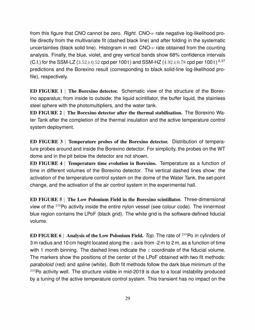
ED FIGURE 1 | The Borexino detector. Schematic view of the structure of the Borex-ino apparatus; from inside to outside: the liquid scintillator, the buffer liquid, the stainlesssteel sphere with the photomultipliers, and the water tank.ED FIGURE 2 | The Borexino detector after the thermal stabilisation. The Borexino Wa-ter Tank after the completion of the thermal insulation and the active temperature controlsystem deployment.

ED FIGURE 3 | Temperature probes of the Borexino detector. Distribution of tempera-ture probes around and inside the Borexino detector. For simplicity, the probes on the WTdome and in the pit below the detector are not shown.ED FIGURE 4 | Temperature time evolution in Borexino. Temperature as a function oftime in different volumes of the Borexino detector. The vertical dashed lines show: theactivation of the temperature control system on the dome of the Water Tank, the set-pointchange, and the activation of the air control system in the experimental hall.

ED FIGURE 5 | The Low Polonium Field in the Borexino scintillator. Three-dimensionalview of the 210Po activity inside the entire nylon vessel (see colour code). The innermostblue region contains the LPoF (black grid). The white grid is the software-defined fiducialvolume.

ED FIGURE 6 | Analysis of the Low Polonium Field. Top. The rate of 210Po in cylinders of3 m radius and 10 cm height located along the z axis from -2 m to 2 m, as a function of timewith 1 month binning. The dashed lines indicate the z coordinate of the fiducial volume.The markers show the positions of the center of the LPoF obtained with two fit methods:paraboloid (red) and spline (white). Both fit methods follow the dark blue minimum of the210Po activity well. The structure visible in mid-2019 is due to a local instability producedby a tuning of the active temperature control system. This transient has no impact on the

29

final result. Bottom. Distribution of 210Po events after the blind alignment of data using thez0 from the paraboloidal fit (red markers in ED Fig. 6 top). The red solid lines indicate theparaboloidal fit within 20 tonnes with Eq. 4.

ED FIGURE 7 | Angular and radial uniformity of the β events in the optimized energy win-dow. Top. Angular power spectrum as a function of the multipole moment l of observedβ events (black points) compared with 104 uniformly distributed events from Monte Carlosimulations at one (dark pink) and two σ C.L. (pink). Data are compatible with a uniformdistribution within the uncertainty of 0.59 cpd per 100 t . Inset : Angular distribution of theβ events. Bottom. Normalized radial distribution of β events r/r0 (black points), wherer0 = 2.5 m is the radius of the sphere surrounding the analysis fiducial volume. The linearfit of the data (red solid line) is shown along with the 1σ (yellow) and 2σ (green) C.L.bands. The data are compatible with a uniform distribution within 0.52 cpd per 100 t .

ED FIGURE 8 | Multivariate fit of the Borexino data: energy distributions. Full multi-variate fit results for the TFC-subtracted (left) and the TFC-tagged (right) energy spectrawith corresponding residuals. In both figures the magenta lines represent the resulting fitfunction, the red line is the CNO neutrino electron recoil spectrum, the green dotted line isthe pep neutrino electron recoil spectrum, the dashed blue line is the 210Bi beta spectrum,and in grey we report the remaining background contributions.

ED FIGURE 9 | Multivariate fit of the Borexino data: radial distribution. Radial distri-bution of events in the multivariate fit. The red line is the resulting fit, the green linerepresents the internal uniform contribution and the blue line shows the non-uniform con-tribution from the external background.

ED FIGURE 10 | Frequentist hypothesis test for the CNO observation. Distribution of thetest statistics q (eq. 5) from Monte Carlo pseudo-data sets. The grey distribution q0 is ob-tained with no CNO simulated data and includes the systematic uncertainty. The blackvertical line represents qdata = 30.05. The corresponding p-value of q0 with respect to qdata

gives the significance of the CNO discovery (>5.0σ at 99% C.L.). For comparison, in blueis the q0 without the systematics. The red histogram represents the expected test statisticsdistribution for injected CNO rate equal to 7.2 cpd per 100 t, i.e. our best fit value.

30

12C

13N

13C 14N

15O

15N 16O

17F

17O(p

,γ)

β+

ν(

13N)

(p, γ)

(p,γ)β

+

ν(

15O)

(p,α)

99.95%

(p, γ)

0.05%

(p,γ

)β

+

ν(

17F)

(p,α)

CNOsub-cycle

I

CNOsub-cycle

II

10−2 10−1 100 101 102

Reaction rate [×1034 s−1]

102 103 104

101

103

105

107

109

1011 pp

pep

7Be7Be

8B

hep

13N

15O

17F

ec13N

ec15O+17F

Neutrino Energy [keV]

Flux

[cm

−2

s−1

(100

keV

)−1]

Figure 1: FIGURE-1

31

Energy [keV]

1

10

210

310

hE

vent

s / 5

N

νCNO-νpep-

Bi210

νB-8 and νBe-7

C11

external backgroundsother backgrounds

Total fit: p-value = 0.3

200 300 400 500 600 700 800 900hN

500 1000 1500 2000 2500

Figure 2: FIGURE-2

32

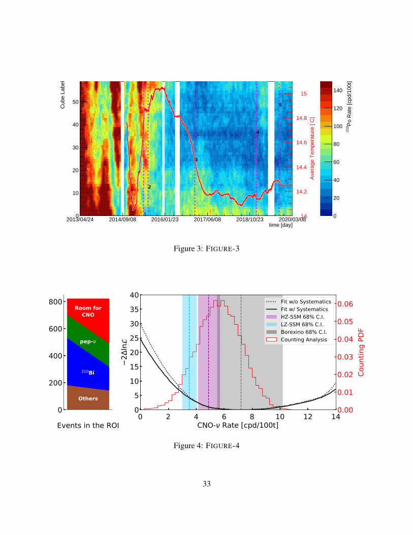
2013/04/24 2014/09/08 2016/01/23 2017/06/08 2018/10/23 2020/03/08 time [day]

0

10

20

30

40

50

Cub

e La

bel

0

20

40

60

80

100

120

140

Po

Rat

e [c

pd/1

00t]

210

1

2

3

4

5

14

14.2

14.4

14.6

14.8

15

C]

°A

vera

ge T

empe

ratu

re [

Figure 3: FIGURE-3

Events in the ROI

0

200

400

600

800Room for

CNO

pep-ν

210Bi

Others

0.00

0.01

0.02

0.03

0.04

0.05

0.06

Coun

ting

PDF

0 2 4 6 8 10 12 14CNO-ν Rate [cpd/100t]

05

10152025303540

−2Δl

n

Fit w/o SystematicsFit w/ SystematicsHZ-SSM 68% C.I.LZ-SSM 68% C.I.Borexino 68% C.I. Counting Analysis

Figure 4: FIGURE-4

33

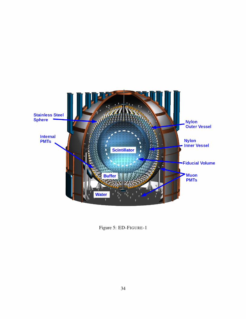
Figure 5: ED-FIGURE-1

34

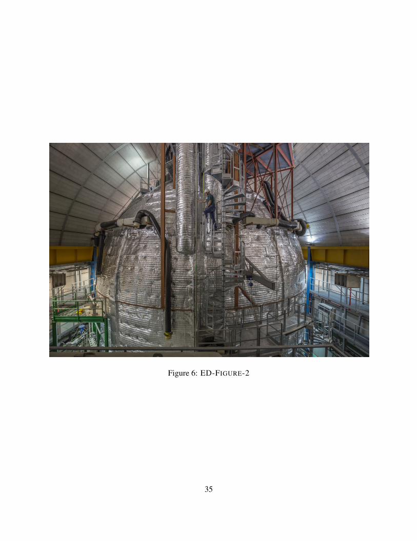
Figure 6: ED-FIGURE-2

35

Figure 7: ED-FIGURE-3

36

Jan-2015 Jan-2016 Jan-2017 Jan-2018 Jan-2019 Jan-202010

11

12

13

14

15

16

17

Tem

pera

ture

(°C)

1 2 3 4 5 6

1 - Beginning of the Insulation 4 - Start of ATCS2 - Water Loop turning OFF 5 - Change of ATCS set-points3 - Completion of the Insulation 6 - Start of Hall C TCS

N1S1N2S2N3S3N4S4N5S5N6S6N7S7

Figure 8: ED-FIGURE-4

37

Figure 9: ED-FIGURE-5

38

Figure 10: ED-FIGURE-6

39

Figure 11: ED-FIGURE-7

40

1

10

210

310

hE

vent

s / 5

N

200 300 400 500 600 700 800 900hN

νCNO- νB-8 and νBe-7

νpep- C11

Bi210 external bkgsTotal fit: p-value = 0.3 other bkgs

1

10

210

310

hE

vent

s / 5

N

200 300 400 500 600 700 800 900hN

4−3−2−1−0

1

2

3

4

Res

idua

ls

500 1000 1500 2000 2500Energy [keV]

4−3−2−1−0

1

2

3

4

Res

idua

ls

500 1000 1500 2000 2500Energy [keV]

Figure 12: ED-FIGURE-8

41

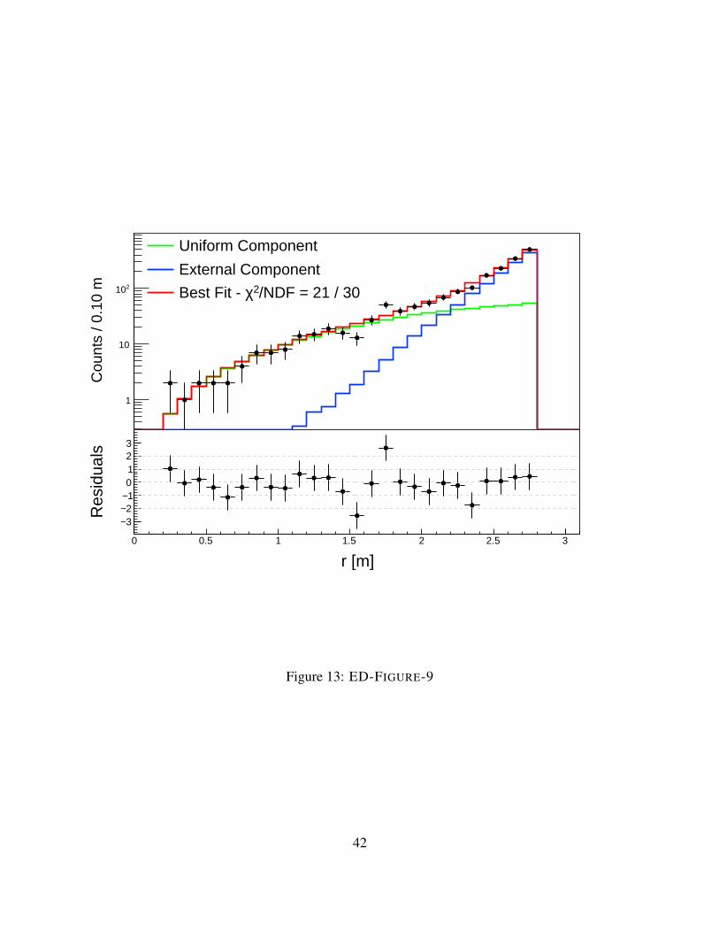
R [m]

1

10

210

Cou

nts

/ 0.1

0 m

Uniform Component

External Component

/NDF = 21 / 302χBest Fit -

0 0.5 1 1.5 2 2.5 3

r [m]

3−2−1−0123

Res

idua

ls

Figure 13: ED-FIGURE-9

42

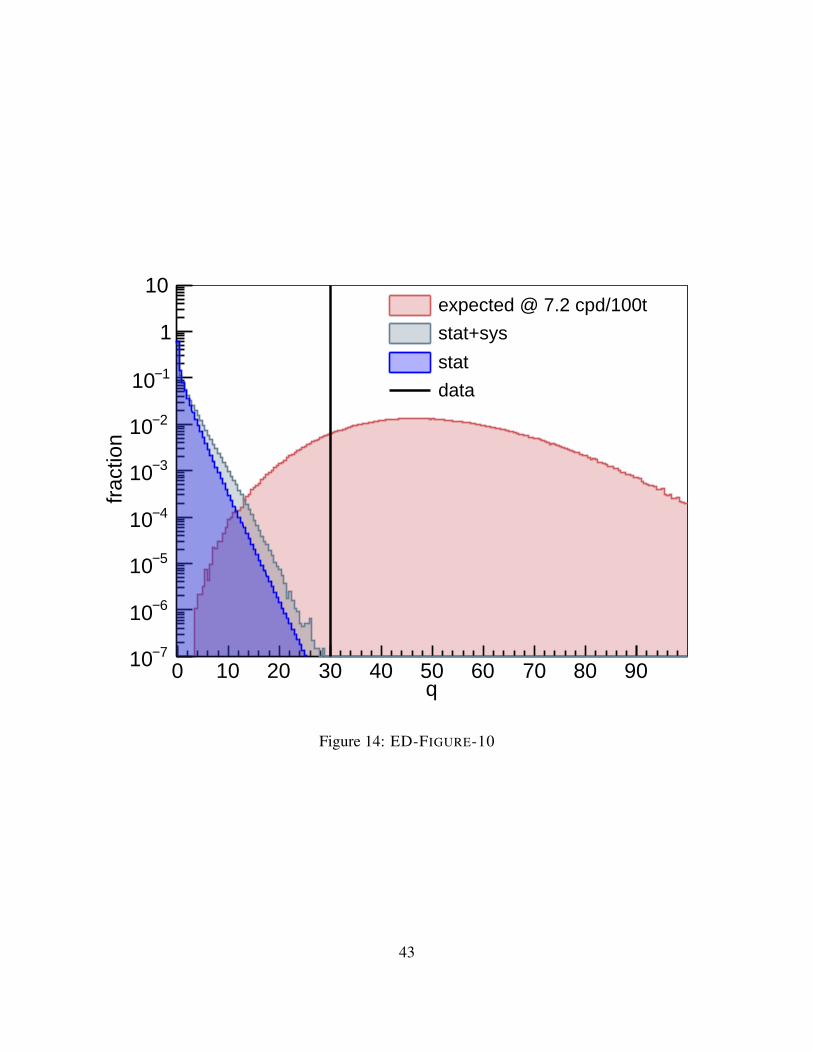
0 10 20 30 40 50 60 70 80 90q

7−10

6−10

5−10

4−10

3−10

2−10

1−10

1

10

frac

tion

expected @ 7.2 cpd/100t

stat+sys

stat

data

Figure 14: ED-FIGURE-10

43