First-arrival traveltime tomography with long- and short-wavelength statics constraints Ziang Li*, Jie Zhang, University of Science and Technology of China (USTC)

Summary Tomographic inversion with statics (TIS) method has been developed to solve jointly for short static corrections and a velocity model. Statics-optimized traveltime tomography (SOTT) produces a velocity model that ensures an effective long-wavelength statics solution at the same time. We combine the two methods to produce a velocity model with both long- and short-wavelength statics accounted for. Applying the TIS method, we first obtain the short-wavelength statics solution and apply that to correct the traveltime picks, and then we invert corrected traveltimes with long-wavelength statics optimization for constraints. The final velocity results fit the data corrected by residual statics and also ensure effectiveness of the long-wavelength statics solution at the same time. We demonstrate the two-step approach with synthetics and real data. For the real data example, CMP stacking results with both the long- and short-wavelength statics applied show improved structure images. Introduction Seismic velocity variations in the near surface area can cause significant long- and short-wavelength statics problems (Taner et al., 1974). It requires to apply static time shifts to solve the problem in seismic data processing. Static corrections compensate for reflection or the refraction distortions introduced by elevation changes and weathering velocities. Near surface imaging may recover the long-wavelength scale of structures accounting for the corrections, subsequent small short-wavelength statics may be solved separately with refraction or reflection data. First-arrival traveltime tomography is one of the near surface imaging approaches for resolving long-wavelength structures, and the corresponding static corrections (Zhu et al., 1992; Zhang and Toksӧz, 1998). Bergman et al. (2004, 2006) develop a tomographic inversion method with short-wavelength statics (TIS) accounted for. They suggest jointly solving short-wavelength static corrections along with the velocity model in tomography studies. Their approach presumably absorbs the short-wavelength near-surface velocity variations (Tryggvason et al., 2009). The approach of TIS is dealing with short-wavelength statics due to partial traveltime misfit that cannot be represented by any long-wavelength velocity model. Zhang (2015) develops statics-optimized traveltime tomography (SOTT), and suggests solving a first-arrival traveltime tomography problem that fits the traveltime data and also minimizes the

traveltime variance in the common-offset domain after applying the long-wavelength static corrections. This method can ensure that the long-wavelength statics solution effectively removes the near surface variances by using traveltime data alone. In this study, we develop a first-arrival traveltime tomography approach with both long- and short-wavelength statics constraints. The long-wavelength statics constraints and the short-wavelength static corrections to the traveltime picks should help reconstructing a more accurate velocity model. We apply the method to both synthetic data and a real dataset acquired in Sichuan, China. The common midpoint (CMP) stacking is performed to verify the effectiveness of the method in the real data test. Method According to Zhang (2015), in SOTT method, the objective function is defined as

22 2( ) ( ) ( ( ) ( )) ( )x off s rG D T T L m d m d m m m (1)

where d is the picked traveltimes, G(m) is calculated traveltimes using model m, doff is the common-offset traveltime data, Ts and Tr are the up-down going source and receiver statics associated with model m, Dx is a first-order derivative operator over distance, L is a Laplacian operator. α and β are the scaling factors for the second and third terms. After applying the Gauss-Newton method, the equation (1) can be written as

( ( ))

( ( ) ( ))

T T T T

T Toff s r

G

T Tx

A A B B L L m A d m

B d m m L Lm

(2)

where

( )=

G

mA

m

2 2( ) ( )s rT T

x x

m mB

m m (3)

We add the short-wavelength static corrections t0 to the traveltime residual term, so the equation (2) can be written as

Traveltime tomography with statics constraints

0( ( ) )

( T ( ) T ( ))

T T T T

T Toff s r

G

x

A A B B L L m A d m t

B d m m L Lm

(4)

In TIS method, the t0 term is solved by singular value decomposition (SVD) method (Pavlis and Booker, 1980). The computed static term t0 can be considered as a surface-consistent term that is a combination of receivers and all involved source-location static shifts (Tryggvason et al., 2009).

I

j j i ii

t r w s (5)

where rj is the receiver static term, si are all the I source static terms involved in computing tj , and wi is a weighting parameter (we use 1 / I for weighting). Thus, our inversion process includes two steps: the first step is to solve the short-wavelength static corrections t0

according to the SVD method and equation (5), the second step is to update the velocity model according to the equation (4). Conjugate gradient algorithm is applied to solve the Gauss-Newton problem. During the inversion process, the selection of weighting factors α and β is important. In this study, we estimate the parameter α and β from several trial-and-error experiments. Synthetic test We apply the traveltime tomography with statics constraints to a 2D synthetic model. Figure 1a shows the true model. It includes both long- and short-wavelength velocity variations and rugged topography. To test the resolving capability of the survey geometry, we choose the similar shot and receiver intervals for the synthetic test as in Sichuan seismic survey that we discuss later, which includes 201 shots with a shot interval of 50 m and 401 receivers for each shot with a receiver interval of 25 m. Figure 1b shows a starting model for the standard traveltime tomography and tomography with statics constraints. Figure 1c shows the near-surface model estimated by first-arrival traveltime tomography. The traveltime tomography results include most of the features of the true model, but the high velocity subjects are not well resolved. The velocity model from the tomography with statics constraints is shown in Figure 1d. The resolution of the high velocity zone is significantly improved and the low velocity zones also show higher contrasts. The short-wavelength statics of shots and receivers are shown in Figure 1e.

a)

b)

c)

d)

Traveltime tomography with statics constraints

e)

Figure 1: Synthetic experiment: a) True model; b) Initial velocity model; c) First-arrival traveltime tomography result; d) Tomography with statics constraints result (Top white curve-Final datum; Bottom white curve-Intermediate datum); e) Short-wavelength statics of shots and receivers.

Figure 2 shows the long-wavelength statics solutions from the traveltime tomography and the statics-optimized tomography. The overall trend is similar, but the two solutions differ in details. Long-wavelength statics from statics-optimized tomography helps flatten COG traveltimes.

Figure 2: Long-wavelength statics based on the traveltime tomography results (blue) and statics-optimized tomography results (red). The solid line denotes the statics of receivers, and the dashed line denotes the statics of shots.

Sichuan data example We process a real 2D dataset from Sichuan, China, with the method presented above. The geometry consists of 194 shots with an average shot interval of 39 m. A total of 445 receiver groups for each shot is placed along a 13 km line at a 30 m interval. Figure 3a shows a starting model for the traveltime tomography and statics-optimized tomography, which is created by picking refraction turning points from the first-

arrival traveltimes. The first-arrival traveltime tomography generates the velocity solution shown in Figure 3b. The results show strong vertical velocity variations below the rugged topography. Figure 3c presents the velocity model inverted from the statics-optimized tomography. The low velocity zone seems to be sharper and more continuous in the very shallow area due to the statics constraints. The short-wavelength statics are shown in Figure 3d. a)

b)

c)

d)

Traveltime tomography with statics constraints

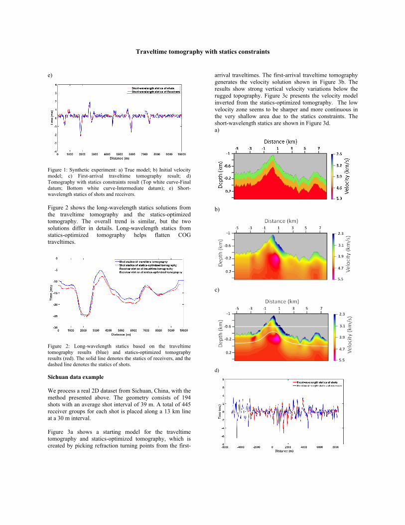
Figure 3: Sichuan data experiment: a) Initial velocity model; b) First-arrival traveltime tomography solution; c) Tomography with statics constraints result (Top white curve-Final datum; Bottom white curve-Intermediate datum); d) Short-wavelength statics of shots and receivers. Figure 4a shows the long-wavelength statics based on the results of the traveltime tomography and statics-optimized tomography. The statics differences are calculated for these two models and are shown in Figure 4b. The major differences are found between 0 and 3 km. a)

b)

Figure 4: a) Long-wavelength statics based on the traveltime tomography results (blue) and statics-optimized tomography results (red). The solid line denotes the statics of receivers, and the dashed line denotes the statics of shots. b) Difference between the long-wavelength statics curves from the shots (red) and receivers (blue) for the two models.

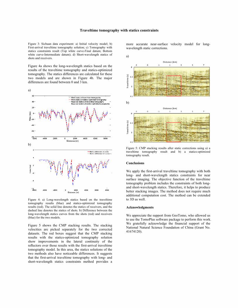
Figure 5 shows the CMP stacking results. The stacking velocities are picked separately for the two corrected datasets. The red boxes suggest that the CMP stacking results with the statics-optimized tomography solution show improvements in the lateral continuity of the reflectors over those results with the first-arrival traveltime tomography model. In this area, the statics solutions of the two methods also have noticeable differences. It suggests that the first-arrival traveltime tomography with long- and short-wavelength statics constraints method provides a

more accurate near-surface velocity model for long-wavelength static corrections. a)

b)

Figure 5: CMP stacking results after static corrections using a) a traveltime tomography result and b) a statics-optimized tomography result.

Conclusions We apply the first-arrival traveltime tomography with both long- and short-wavelength statics constraints for near surface imaging. The objective function of the traveltime tomography problem includes the constraints of both long- and short-wavelength statics. Therefore, it helps to produce better stacking images. The method does not require much additional computation cost. The method can be extended to 3D as well. Acknowledgments We appreciate the support from GeoTomo, who allowed us to use the TomoPlus software package to perform this work. We gratefully acknowledge the financial support of the National Natural Science Foundation of China (Grant No. 41674120).