Firm’s Problem - UCLA Economics Homepage - UCLA …€™s Problem Simon Board⁄ This Version: September 20, 2009 First Version: December, 2009. In these notes we address the ﬂrm’s

Firm’s Problem

Simon Board∗

This Version: September 20, 2009

First Version: December, 2009.

In these notes we address the firm’s problem. We can break the firm’s problem into threequestions.

1. Which combinations of inputs produce a given level of output?

2. Given input prices, what is the cheapest way to attain a certain output?

3. Given output prices, how much output should the firm produce?

We study the firm’s technology in Sections 1–2, the cost minimisation problem in Section 3 andthe profit maximisation problem in Section 4.

1 Technology

1.1 Model

We model a firm as a production function that turns inputs into outputs. We assume:

1. The firm produces a single output q ∈ <+. One can generalise the model to allow forfirms which make multiple products, but this is beyond this course.

∗Department of Economics, UCLA. http://www.econ.ucla.edu/sboard/. Please email suggestions and typosto [email protected].

1

Eco11, Fall 2009 Simon Board

2. The firm has N possible inputs, {z1, . . . , zN}, where zi ∈ <+ for each i. We normallyassume N = 2, but nothing depends on this. We can think of inputs as labour, capital orraw materials.

3. Inputs are mapped into output by a production function q = f(z1, z2). This is normallyassumed to be concave and monotone. We discuss these properties later.

To illustrate the model, we can consider a farmer’s technology. In this case, the output is thefarmer’s produce (e.g. corn) while the inputs are labour and capital (i.e. machinery). There isclearly a tradeoff between these two inputs: in the developing world, farmers use little capital,doing many tasks by hand; in the developed world, farmers use large machines to plant seedsand even pick fruit.

In some examples inputs may be close substitutes. To illustrate, suppose two students areworking on a homework. In this case the output equals the number of problems solved, whilethe inputs are the hours of the two students. The inputs are close substitutes if all that mattersis the total number of hours worked (see Section 2.3).

In other cases inputs may be complements. To illustrate, suppose an MBA and a computerengineer are setting up a company. Each worker has specialised skills and neither can do theother’s job. In this case, output depends on which worker is doing the least work, and we saythe inputs are perfect compliments (see Section 2.2).

The marginal product of input zi is the output from one extra unit of good i.

MPi(z1, z2) =∂f(z1, z2)

∂zi,

The average product of input i is

APi(z1, z2) =f(z1, z2)

zi.

1.2 Isoquants

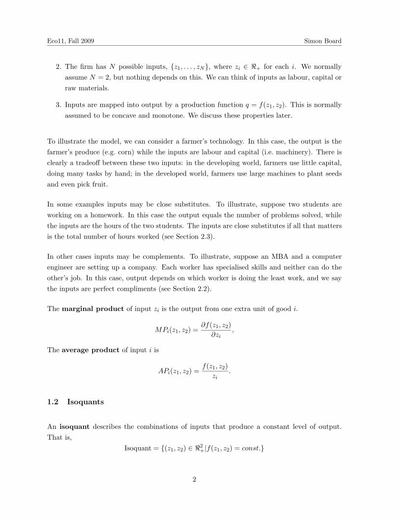
An isoquant describes the combinations of inputs that produce a constant level of output.That is,

Isoquant = {(z1, z2) ∈ <2+|f(z1, z2) = const.}

2


Figure 1: Isoquant. This figure shows two isoquants. Each curve depicts the bundles that yieldconstant output.

A firm has a collection of isoquants, each one corresponding to a different level of output. Byvarying this level, we can trace out the agent’s entire production possibilities.

To illustrate, suppose a firm has production technology

f(z1, z2) = z1/31 z

1/32

Then the isoquant satisfies the equation z1/31 z

1/32 = k. Rearranging, we can solve for z2, yielding

z2 =k3

z1(1.1)

which is the equation of a hyperbola. This function is plotted in figure 1.

1.3 Marginal Rate of Technical Substitution

The slope of the isoquant measures the rate at which the agent is willing to substitute one goodfor another. This slope is called the marginal rate of technical substitution or MRTS.Mathematically,

MRTS = −dz2

dz1

∣∣∣f(z1,z2)=const.

(1.2)

3


We can rephrase this definition in words: the MRTS equals the number of z2 the firm canexchange for one unit of z1 in order to keep output constant.

The MRTS can be related to the firm’s production function. Let us consider the effect of asmall change in the firm’s inputs. Totally differentiating the production function f(z1, z2) weobtain

dq =∂f(z1, z2)

∂z1dz1 +

∂f(z1, z2)∂z2

dz2 (1.3)

Equation (1.3) says that the firm’s output increases by the marginal product of input 1 timesthe increase in input 1 plus the marginal product of input 2 times the increase in input 2. Alongan isoquant dq = 0, so equation (1.3) becomes

∂f(z1, z2)∂z1

dz1 +∂f(z1, z2)

∂z2dz2 = 0

Rearranging,

−dz2

dz1=

∂f(z1, z2)/∂z1

∂u(z1, z2)/∂z2

Equation (1.2) therefore implies that

MRTS =MP1

MP2(1.4)

The intuition behind equation (1.4) is as follows. Using the definition of MRTS, one unit of z1

is worth MRTS units of z2. That is, MP1 = MRTS×MP2. Rewriting this equation we obtain(1.4).

1.4 Properties of Technology

In this section we present three properties of production functions that will prove useful.

1. Monotonicity. The production function is monotone if for any two input bundles z = (z1, z2)and z′ = (z′1, z

′2),

zi ≥ z′i for each i }implies f(z1, z2) > f(z′1, z

′2).

zi > z′i for some i

In words: the production function is monotone if more of any input strictly increases thefirm’s output. Monotonicity implies that isoquants are thin and downwards sloping (see thePreferences Notes). As a result, it implies that MRTS is positive.

4


2. Quasi–concavity. Let z = (z1, z2) and z′ = (z′1, z′2). The production function is quasi–concave

if whenever f(z) ≥ f(z′) then

f(tz + (1− t)z′) ≥ f(z′) for all t ∈ [0, 1] (1.5)

Suppose z and z′ are two input bundles that produce the same output, f(z) = f(z′). Then(1.5) says a mixture of these bundles produces even more output. That is, mixtures of inputsare better than extremes.

Under the assumption of monotonicity, quasi–concavity says that isoquants are convex. Thismeans that the MRTS decreasing in z1 along the isoquant. Formally, an isoquant defines animplicit relationship between z1 and z2,

f(z1, z2(z1)) = k

Convexity then implies that MRTS(z1, z2(z1)) is decreasing in z1. This is illustrated in Pref-erences Notes.

3. Returns to Scale. A production function has decreasing returns to scale if

f(tz1, tz2) ≤ tf(z1, z2) for t ≥ 1 (1.6)

so that doubling the inputs less that doubles the output. A production function has constant

returns to scale iff(tz1, tz2) = tf(z1, z2) for t ≥ 1

so that doubling the inputs also doubles output. Finally, a production function has increasing

returns to scale iff(tz1, tz2) ≥ tf(z1, z2) for t ≥ 1

so that doubling the inputs more than doubles the output.

We will sometimes use the assumption that the production function f(z1, z2) is concave. Thatis, for z = (z1, z2) and z′ = (z′1, z

′2),

f(tz + (1− t)z′) ≥ tf(z) + (1− t)f(z′) for t ∈ [0, 1] (1.7)

Concavity implies that the production function is quasi–concave (1.5) and hence that isoquantsare convex. This follows immediately from definitions: if f(z) ≥ f(z′) then concavity (1.7)

5


impliesf(tz + (1− t)z′) ≥ tf(z) + (1− t)f(z′) ≥ f(z′)

so the production function is quasi–concave. In addition, concavity implies decreasing returnsto scale. Applying the definition of concavity (1.7) to the points z = sz′′ and z′ = 0 for s ≥ 1,and letting t = 1/s, we obtain

f

(1s(sz) +

(1− 1

s

)0)≥ 1

sf(sz) +

(1− 1

s

)f(0)

Using f(0) = 0 and simplifying, we obtain (1.7)

2 Examples of Production Functions

Here we present some examples of production functions. Many details are omitted since this arepetition of the examples of utility functions.

2.1 Cobb Douglas

A Cobb–Douglas production function is given by

f(z1, z2) = zα1 zβ

2 for α ≥ 0 and β ≥ 0

Typical isoquants are shown in figure 1. The marginal products are given by

MP1 = αzα−11 zβ

2

MP2 = βzα1 zβ−1

2

The marginal rate of technical substitution is

MRTS =MP1

MP2=

αz2

βz1

The returns to scale are easy to evaluate.

f(tz1, tz2) = (tz1)α(tz2)βt = tα+βzα1 zβ

2 = tα+βf(z1, z2)

6


Figure 2: Isoquants for Leontief Technology. The isoquants are L–shaped, with the kink along theline αz1 = βz2.

Hence there are decreasing returns if α + β ≤ 1, constant returns if α + β = 1 and increasingreturns if α + β ≥ 1.

Exercise: Assume α + β ≤ 1. Show that f(z1, z2) is concave.1

2.2 Perfect Complements (Leontief)

A Leontief production function is given by

f(z1, z2) = min{αz1, βz2}

The isoquants are shown in figure 2. These are L–shaped with a kink along the line αz1 = βz2.This production function exhibits constant returns to scale.

2.3 Perfect Substitutes

With perfect substitutes, the production function is given by

f(z1, z2) = αz1 + βz2

1For the definition of concavity with two variables, see the p. 5–6 of the math notes.

7


Figure 3: Isoquants for Perfect Substitutes. The isoquants are straight line with slope −α/β.

The isoquants are shown in figure 3. These are straight lines with slope −α/β. This productionfunction exhibits constant returns to scale.

3 Cost Minimisation Problem (CMP)

We make several assumptions:

1. There are N inputs. For much of the analysis we assume N = 2 but nothing depends onthis.

2. The agent takes input prices as exogenous. We assume these prices are linear and strictlypositive and denote them by {r1, . . . , rN}.

3. The firm has production technology f(z1, z2). We normally assume that the productionfunction is differentiable, which ensures that any optimal solution satisfies the Kuhn–Tucker conditions. If the production function is quasi–concave and MPi(z1, z2) > 0 forall (z1, z2), then any solutions to the Kuhn–Tucker conditions are optimal. See Section4.1 of the UMP notes for more details.

8


3.1 Cost Minimisation Problem

The cost minimisation problem is

minz1,...,zN

N∑

i=1

rizi subject to f(z1, . . . , zN ) ≥ q (3.1)

zi ≥ 0 for all i

The idea is that the firm is trying to find the cheapest way to attain a certain output, q. Thesolution to this problem yields the firm’s input demands which are denoted by

z∗i (r1, . . . , rN , q)

The money the firm must spend in order to attain its target output is its cost. The cost

function is therefore

c(r1, . . . , rN , q) = minz1,...,zN

N∑

i=1

rizi subject to f(z1, . . . , zN ) ≥ q

zi ≥ 0 for all i

Equivalently, the cost function equals the amount the firm spends on her optimal inputs,

c(r1, . . . , rN , q) =N∑

i=1

riz∗i (r1, . . . , rN , q) (3.2)

Note this problem is formally identical to the agent’s expenditure minimisation problem. Thecost function is therefore equivalent to the agent’s expenditure function.

Given a cost function, the average cost is,

AC(r1, r2, q) =c(r1, r2, q)

q

The marginal cost equals the cost of each additional unit,

MC(r1, r2, q) =dc(r1, r2, q)

dq

9


Figure 4: Constraint Set. This figure shows the set of inputs that deliver the target output, q.

3.2 Graphical Solution

The firm wishes to find the cheapest way to attain a certain output.

First, we need to understand the constraint set. The firm can choose any bundle of inputswhere (a) the firm attains her target output, f(z1, z2) ≥ q; and (b) the quantities are positive,z1 ≥ 0 and z2 ≥ 0. If the firm’s production function is monotone, then the bundles that meetthese conditions are the ones that lie above the isoquant with output q. See figure 4.

Second, we need to understand the objective. The firm wishes to pick the bundle in theconstraint set that minimises her cost. Define an isocost curve by the bundles of z1 and z2 thatdeliver constant cost:

{(z1, z2) : r1z1 + r2z2 = const.}

These isocost curves are just like budget curves and so have slope −r1/r2. See figure 5.

Ignoring boundary problems and kinks, the solution to the CMP has the feature that the isocostcurve is tangent to the target isoquant. As a result, their slopes are identical. The tangencycondition can thus be written as

MRTS =r1

r2(3.3)

This is illustrated in figure 6.

10


Figure 5: Isocost. The isocost function shows the set of inputs which cost the same amount of money.

Figure 6: Tangency. This figure shows that, at the optimal input combination, the isocost curve istangent to the isoquant.

11


The intuition behind (3.3) is as follows. Using the fact that MRTS = MP1/MP2, equation(3.3) implies that

MP1

MP2=

r1

r1(3.4)

Rewriting (3.4) we find

r1

MP1=

r2

MP1

The ratio ri/MPi measures the cost of increasing output by one unit. At the optimum the agentequates the cost–per–unit of the two goods. Intuitively, if good 1 has a higher cost–per–unitthan good 2, then the agent should spend less on good 1 and more on good 2. In doing so, shecould attain the same output at a lower cost.

If the production function is monotone, then the constraint will bind,

f(z1, z2) = q. (3.5)

The tangency equation (3.4) and constraint equation (3.5) can then be used to solve for thetwo input demands. In addition, one can derive the cost function using equation (3.2).

If there are N inputs, the agent will equalise the cost–per–unit from each good, giving us N −1equations. Using the constraint equation (3.5), we can again solve for the firm’s input demands.

3.3 Example: Cobb Douglas

Suppose a firm has production function f(z1, z2) = z1/31 z

1/32 . The MRTS is

MRTS =13z−2/31 z

1/32

13z

1/31 z

−2/32

=z2

z1

The tangency condition from the CMP is thus

r1

r2=

z2

z1

Rewriting, this says r1z1 = r2z2, so the firm spends the same on both its inputs.

12


Figure 7: Cost curves. This figure shows the cost, average cost and marginal cost curves for theCobb–Douglas example.

The constraint equation is q = z1/31 z

1/32 . This means that

q3 = z1z2 = z1r1z1

r2

where the second equality uses the tangency condition. Rearranging, we find the optimal inputdemands are

z∗1 =(

r1

r2

)1/2

q3/2 and z∗2 =(

r2

r1

)1/2

q3/2

The cost function isc(r1, r2, q) = r1z

∗1 + r2z

∗2 = 2(r1r2)1/2q3/2

The average and marginal costs are

AC(r1, r2, q) = 2(r1r2)1/2q1/2 and MC(r1, r2, q) = 3(r1r2)1/2q1/2

These are illustrated in figure 7.

3.4 Lagrangian Solution

Using a Lagrangian, we can encode the tangency conditions into one formula. As before, let usignore boundary problems. The CMP can be expressed as minimising the Lagrangian

L = r1z1 + r2z2 + λ[q − f(z1, z2)]

13


As usual, the term in brackets can be thought as the penalty for violating the constraint. Thatis, the firm is punished for falling short of the target output.

The FOCs with respect to z1 and z2 are

∂L

∂z1= r1 − λ

∂u

∂z1= 0 (3.6)

∂L

∂z2= r2 − λ

∂u

∂z2= 0 (3.7)

If the production function is monotone then the constraint will bind,

f(z1, z2) = q (3.8)

These three equations can then be used to solve for the three unknowns: z1, z2 and λ.

Several remarks are in order. First, this approach is identical to the graphical approach. Di-viding (3.6) by (3.7) yields

∂u/∂z1

∂u/∂z2=

r1

r2

which is the same as (3.4). Moreover, the Lagrange multiplier is exactly the cost–per–unit,

λ =r1

MP1=

r2

MP2.

Second, if preferences are not monotone, the constraint (3.5) may not bind. If it does not bind,the Lagrange multiplier in the FOCs will be zero.

Third, the approach is easy to extend to N inputs. In this case, one obtains N first–orderconditions and the constraint equation (3.5).

3.5 Properties of Cost Functions

We now develop six properties of the cost function. The first four are identical to the propertiesof the expenditure function: see the EMP Notes for more details.

1. The cost function is homogenous of degree one in prices. That is,

c(r1, r2, q) = c(tp1, tp2, q) for t > 0

14


Figure 8: Concavity of Cost Function in Input Prices. This figure shows how the cost functionlies under the pseudo–cost function.

Intuitively, if the prices of r1 and r2 double, then the cheapest way to attain the target outputdoes not change. However, the cost of attaining this output doubles.

2. The cost function is increasing in (r1, r2, q). If we increase the target output then theconstraint becomes harder to satisfy and the cost of attaining the target increases. If weincrease r1 then it costs more to buy any bundle of inputs and it costs more to attain the targetoutput.

3. The cost function is concave in input prices (r1, r2). Fix the target utility q and prices(r1, r2) = (r′1, r

′2). Solving the CMP we obtain input demands z′1 = z∗1(r

′1, r

′2, q) and z′2 =

z∗2(r′1, r

′2, q). Now suppose we fix demands and change r1, the price of input 1. This gives us a

pseudo–cost functioncz′1,z′2(p1) = r1z

′1 + r′2z

′2

which is linear in r1. Of course, as r1 rises the firm can reduce her costs by rebalancing herinput demand towards the input that is cheaper. This means that real cost function lies belowthe pseudo–cost function and is therefore concave. See figure 8.

4. Sheppard’s Lemma: The derivative of the cost function equals the input demand. That is,

∂

∂r1c(r1, r2, q) = z∗1(r1, r2, q) (3.9)

The idea behind this result can be seen from figure 8. At r1 = r′1 the cost function is tangential

15


to the pseudo–cost function. The pseudo–cost is linear in r1 with slope z∗1(r′1, r

′2, q), so the

expenditure function also has slope z∗1(r′1, r

′2, q).

The intuition behind Sheppard’s Lemma is as follows. When r1 increases by ∆r1 there aretwo effects. First, holding input demand constant, the firm’s cost rises by z∗1(r1, r2, q) ×∆r1.Second, the firm rebalances its demands, buying less of input 1 and more of input 2. However,this has a small effect on the firm’s costs since it is close to indifferent buying the optimalquantity and nearby quantities.

5. If f(z1, z2) is concave then c(r1, r2, q) is convex in q. Intuitively, concavity of the productionfunction, implies that the marginal product of an input is decreasing in the amount of the inputused:

d

dziMPi(z1, z2) =

d2

dz2i

f(z1, z2) ≤ 0

Therefore, as the firm expands, it needs more inputs to produce each additional unit of output.As a result, the cost of producing this unit increases, and the total cost is convex. When thereis only one input this is easy to see formally: if f(z) is concave, then c(q) = rf−1(q) is convex.

6. AC(q) is increasing when MC(q) ≥ AC(q), is flat when MC(q) = AC(q) and is anddecreasing when MC(q) ≤ AC(q). Suppose the firm currently produces n units of output, andthat the marginal cost of the (n + 1)st unit is higher than the average cost of the first n. Thenthe average cost of producing n + 1 units is higher that producing n units since the costs isbeing dragged up by the final unit. To prove this result formally, we can differentiate the AC

curve,d

dqAC(q) =

d

dq

c(q)q

=c′(q)q − c(q)

q2

Hence AC(q) is increasing if and only if c′(q)q ≥ c(q). Rearranging, this condition is justMC(q) ≥ AC(q), as required.

3.6 Pictures of Cost Functions

Figure 7 shows the cost curves associated with a concave production function. One can seethat the cost function is convex and, as a result, the marginal cost is increasing and exceedsthe average cost.

Figure 9 shows the cost curves associated with a production function which is concave for

16


Figure 9: Cost Curves for a Nonconcave Production Function I: Fixed Cost. This figureshows the cost, average cost and marginal cost curves when the firm must pay a fixed cost.

positive quantities but requires a fixed cost needed to initiate production.2 The marginal costof the first unit is infinite and is therefore not shown in the picture; the marginal cost of eachsubsequent unit is increasing. The average cost is U–shaped: it starts at infinity, is minimised atq′ and then rises as the higher marginal cost drags up the average cost. Note that the marginalcost intersects the average cost at its lowest point: this follows from property 6 from Section3.5.

Figure 10 shows the cost curves associated with a second nonconcave production function.3

The cost curve is S–shaped. As a result, the marginal cost and average cost functions are U–shaped. For the first unit, the marginal cost and average cost coincide; for low levels of output,the marginal cost is decreasing and lies below the average cost; for high levels of output, themarginal cost is increasing, exceeding the average cost for q ≥ q′.

3.7 Long Run vs. Short Run Costs

The cost of a firm depend on which factors of production are flexible. We differentiate betweenfour cases, and then illustrate them with an example.4

2For example, try f(z) = (z − 1)1/2.3For example, try f(z) = 100z − 16z2 + z3.4While the idea of short and long run is standard, different authors mean different things by the “short run”

and “long run”.

17


Figure 10: Cost Curves for a Nonconcave Production Function II. This figure shows the cost,average cost and marginal cost curves.

1. In the very short run all the factors of production are fixed, and output is fixed.

2. In the short run some factors are flexible, while others are fixed. For example, thefirm may be able hire some more workers, but may not be able to order new capitalequipment. Any fixed costs are also sunk, so that they cannot be avoided even if the firmceases production.

3. In the medium run all factors are flexible, but fixed costs are sunk.

4. In the long run all factors are flexible and fixed costs are not sunk. Hence the firm cancostlessly exit.

In practice, the meaning of short and long run depend on the application. For example, considera farmer who wishes to increase her output. It may take her a few days to hire an extra worker,a few weeks to lease an extra tractor and a few months for a new farmer to buy land and enterthe business (or for an old one to exit).

To illustrate, suppose a firm has production function5

f(z1, z2) = (z1 − 1)1/3(z2 − 1)1/3

This firm has Cobb–Douglas production, except that the first unit of both inputs is useless,inducing a fixed cost.

5Since negative outputs are impossible, we should say that q = 0 if either z1 < 1 or z2 < 1.

18


First, let us solve for the long–run cost function. The firm’s Lagrangian is

L = r1z1 + r1z2 + λ[q − (z1 − 1)1/3(z2 − 1)1/3]

Differentiating, this induces the tangency condition r1(z1−1) = r2(z2−1). Using the constraint,q = (z1 − 1)1/3(z2 − 1)1/3 − 1, we obtain

z∗1 =(

r1

r2

)1/2

(q)3/2 + 1 and z∗2 =(

r2

r1

)1/2

(q)3/2 + 1

The cost function is

c(r1, r2, q) = r1z∗1 + r2z

∗2 = 2(r1r2)1/2(q)3/2 + (r1 + r2)

In addition, the firm can shutdown and produce zero at cost c(r1, r2, 0) = 0. Observe that thiscost function is the same as that in Section 3.3 with a startup cost of r1 + r2.

In the medium run, the fixed cost r1 + r2 is sunk. The medium run cost curve is therefore

c(r1, r2, q) = 2(r1r2)1/2(q)3/2 + (r1 + r2)

where c(r1, r2, 0) = r1 + r2.

In the short run, z1 is flexible but z2 is fixed at z′2. The fixed cost is also sunk. The constraintin the CMP becomes

q = (z1 − 1)1/3(z′2 − 1)1/3

Rearranging,

z∗1 =q3

z′2 − 1+ 1

The cost function is therefore given by

c(r1, r2, q; z′2) = r1z∗1 + r2z

′2 = r1

q3

z′2 − 1+ r1 + r2z

′2

Figure 11 illustrates the short run cost curves for three different levels of z2. Observe that thelong run cost curve is given by the lower envelope of the short run cost curves. To see why thisis the case, fix an output level q′ and calculate the optimal input demands when both factors areflexible, denoted by z′1 and z′2. Now suppose we fix z2 at z′2 and consider the cost of attainingdifferent output levels. If q = q′ then the firm is using the optimal amount of input 2 and theshort–run cost will coincide with the long–run cost. If q > q′ then the firm is using too little of

19


Figure 11: Long Run and Short Run Costs. This figure shows the long run cost curve and theshort run cost curves corresponding to three levels of the second input.

z2 and too much of z1, raising the short–run cost over the long–run cost. If q < q′ then the firmis using too much of z2 and too little of z1, again raising the short–run cost over the long–runcost.

In the very short run, inputs are fixed at z1 = z′1 and z2 = z′2. Hence the firm can produceq′ = (z′1 − 1)1/3(z′2 − 1)1/3 at cost r1z

′1 + r1z

′2, but is unable to produce anything else.

4 Profit Maximisation Problem (PMP)

Assumptions:

1. There is one output good, with linear price p. This means that the firm is a price–takerin the output market.

2. There are two input goods with linear prices r1 and r2. The firm is therefore a price–takerin the input market.

3. The firm has production technology f(z1, z2). We normally assume that the productionfunction is differentiable, which ensures that any optimal solution satisfies the first–orderconditions.

20


The firm’s profit equals its revenue from selling the output minus it’s cost:

π = pf(z1, z2)− r1z1 − r2z2

We now explore two ways of solving this problem.

4.1 One–Step Solution

The firm’s profit maximisation problem is

maxz1,z2

pf(z1, z2)− r1z1 − r2z2 subject to zi ≥ 0 for all i (4.1)

The first–order conditions are

dπ

dz1= p

∂f(z1, z2)∂z1

− r1 = 0 (4.2)

dπ

dz2= p

∂f(z1, z2)∂z2

− r2 = 0 (4.3)

Together (4.2) and (4.3) define the optimal input demands of the firm, z∗1(p, r1, r2) and z∗2(p, r1, r2).we can then derive the optimal output:

q∗(p, r1, r2) = f(z∗1 , z∗2)

which is called the supply function. We can also derive the firm’s optimal profit,

π∗(p, r1, r2) = pq∗ − r1z∗1 − r2z

∗2

which is called the profit function.

Observe that solving (4.1) is much easier than solving the utility maximisation problem. Withthe UMP, the consumer maximises her utility subject to spending no more than her income.With the PMP, the firm’s expenses directly enter the firm’s objective function, so we only haveto solve an unconstrained optimisation problem.

In order for the FOCs (4.2) and (4.3) to characterise a maximum, the second–order conditions

21


must hold. That is, f(z1, z2) must be locally concave, which implies

∂2

∂z21

f(z1, z2) =∂

∂z1MP1(z1, z2) ≤ 0

∂2

∂z22

f(z1, z2) =∂

∂z2MP2(z1, z2) ≤ 0

If f(z1, z2) is globally concave, then any solution to the FOCs is a maximum.


Suppose a firm has production function f = z1/31 z

1/32 . Profit is given by

π = pz1/31 z

1/32 − r1z1 − r2z2

The FOCs are

13pz−2/31 z

1/32 = r1

13pz

1/31 z

−2/32 = r2

Solving these two equations yields input demands:

z∗1(p, r1, r2) =127

p3

r21r2

and z∗2(p, r1, r2) =127

p3

r1r22

The optimal supply is

q∗(p, r1, r2) = (z∗1)1/3(z∗2)

1/3 =19

p2

r1r2

The profit function is

π∗(p, r1, r2) = pq∗ − r1z∗1 − r2z

∗2 =

127

p3

r1r2

4.3 Two–Step Solution

Step 1. Find the cheapest way to attain output q. Recall the cost function is given by

c(q, r1, r2) = minz1,z2

r1z1 + r2z2 subject to f(z1, z2) ≥ q

zi ≥ 0 for all i

22


Step 2. Find the profit–maximising output. Given a cost function, the firm’s problem is

maxq

π = pq − c(q, r1, r2) subject to q ≥ 0

The first–order condition for this problem is

dπ

dq= p− d

dqc(q, r1, r2) = 0

That is,

p = MC(q, r1, r2) (4.4)

The idea behind this result is shown in the left panel of figure 12, which shows the firm’s revenueand costs as a function of output, q. The firm wishes to maximise the vertical distance betweenthe two lines so, at the optimum, they are parallel. The slope of the revenue line is p while theslope of the cost function is MC, which yields (4.4).

One can also look at this result with the right panel of figure 12. The difference p − MC

equals the profit the firm makes on the last unit. The FOC (4.4) says that the firm will keepproducing while the profit–per–unit is positive and will stop when it falls to zero. Note that, inthis picture, one can measure profits two ways. First, profit equals the price obtained per unitminus the average cost of a unit multiplied by the number of units sold:

π(q) = pq − c(q) = pq −AC(q)q = [p−AC(q)]q

In the picture, this equals the areas given by A+B+C.

Second, the profit of a marginal unit is p−MC(q). Hence the total profit of the firm, ignoringfixed costs, is the area below the price and above the MR curve. That is,

π(q) = pq − c(q) =∫ q

0pdq̃ −

∫ q

0MC(q̃)dq̃ − F =

∫ q

0[p−MC(q̃)] dq̃ − F

where F is the fixed cost. Hence the firm’s profit is A+B+D+E minus the fixed cost, F .

In order for the FOC (4.4) to constitute an optimum, the second–order condition should hold:

d2π

dq2= − d2

dq2c(q, r1, r2) = − d

dqMC(q, r1, r2) ≤ 0

So the marginal cost needs to be locally increasing. Conversely, if the cost function is convex,

23


Figure 12: Profit maximisation. The left panel shows that profit is maximised when the revenue lineis parallel to the cost line. The vertical gap, is then equal to the firm’s profit. The right panel showsthat profit is maximised when the price equals to marginal cost. Profit then equals A+B+C.

which is guaranteed by the concavity of f(z1, z2), then any solution to the FOC (4.4) is anoptimum.


We now return to the example in Section 4.2, deriving the same results using the two–stepapproach.

Suppose f(z1, z2) = z1/31 z

1/32 . Using the results in Section 3.3, the cost function is

c(q, r1, r2) = 2(r1r2)1/2q3/2

The first–order condition (4.4) yields

p = 3(r1r2q)1/2

Rearranging, the supply curve is given by

q∗(p, r1, r2) =19

p2

r1r2

24


The profit function is then

π∗(p, r1, r2) = pq∗ − r1z∗1 − r2z

∗2 =

127

p3

r1r2

as in Section 4.2.

4.5 Examples of Supply Functions

Figure 13 shows the supply function that results from a convex cost function with no fixedcost.6 The marginal cost is increasing and is always above the average cost. For any givenprice, the firm chooses quantity such that p = MC(p). Hence the supply curve coincides withthe MC curve.

Figure 14 shows the supply function that results from a convex cost function with a fixed cost.7

The marginal cost function is increasing so, if the firm produces, its supply curve coincides withMC(q). However, when the price lies below the average cost, the firm makes negative profits.Hence the firm’s supply curve coincides with the MC(q) curve above the AC(q) curve and iszero elsewhere.

Figure 15 shows the supply function that results from a U–shaped marginal cost functionwithout a fixed cost.8 For prices below p′ the marginal cost is below the average cost, so thefirm cannot make a profit and it chooses to produce q∗(p) = 0. At p = p′ the firm is indifferentbetween producing 0 and q′. For price above p′ the firm produces on the increasing part of themarginal cost function.

Figure 16 shows the supply function that results from a nonconvex cost curve.9 For low pricesthe supply curve coincides with the first part of the MC curve. At a price p′ the supply jumpsto the right. Intuitively, if the firm is going to pay to produce the expensive units in region Athen it should also produce the cheap units in region B. At the optimum, the area of A equalsthe area of B, so the profit lost by producing the expensive units is exactly offset by the profitgained by producing the cheap units.

One can also use these figures to understand the difference between the short–run and long–run supply curves. In the very short run, supply is fixed and the supply curve is vertical. In

6For example, try c(q) = q + q2.7For example, try c(q) = 1 + q + q2.8For example, try c(q) = 15q − 12q2 + q3.9For example, try c(q) = 20q2 − 8q3 + q4.

25


Figure 13: Supply Curve with Convex Costs. This figure shows how the supply curve coincideswith the marginal cost curve.

Figure 14: Supply Curve with Nonconvex Costs I: Fixed Costs. This figure shows how thesupply curve coincides with the marginal cost curve when it lies above the average cost.

26


Figure 15: Supply Curve with Nonconvex Costs II: U–Shaped Marginal Cost. This figureshows how the supply curve coincides with the marginal cost curve when it lies above the average cost.

Figure 16: Supply Curve with Nonconvex Costs III. This figure shows how the supply curvecoincides with the marginal cost curve when it lies above the average cost.

27


the short–run, some of the inputs are fixed and the supply curve coincides with the short–runmarginal cost. In the medium–run, the firm can change all its inputs, but cannot close down.Hence the supply curve coincides with the marginal cost curve above the average variable cost.In the long–run the firm can shut down, so the supply curve coincides with the marginal costabove the average cost.

4.6 Properties of the Profit Function

The profit function π∗(p, r1, r2) has four key properties:

1. π∗(p, r1, r2) is homogenous of degree one in (p, r1, r2). If all prices double then the opti-mal production choices remain unchanged and profit also doubles. Intuitively, if currency isdenominated in a different currency this should not affect the firm’s choices.

2. π∗(p, r1, r2) is increasing in p and decreasing in (r1, r2). An increase in p increases profitsfor any output q, and therefore increases profit for the optimal output choice. An increase inr1 increases costs and decreases profits for any output q, and therefore decreases profit for theoptimal output choice.

3. π∗(p, r1, r2) is convex in (p, r1, r2). Let us first consider changes in p, and ignore the inputprices. Fix p = p′ and solve for the optimal output q′ = q∗(p′). Now suppose we fix the outputand change p, yielding a pseudo–profit function pq′ − c(q′) which is linear in p. Of course, asp rises the firm can increase her output, so the real cost function lies above this straight lineand is therefore convex. See figure 16. Second, the profit function is convex in (r1, r2) becauseprofit is equal π = pq − c(q, r1, r2) and c(q, r1, r2) is concave in (r1, r2).

4. Hotelling’s Lemma: The derivative of the profit function with respect to the output priceequals the optimal output. That is,

∂

∂pπ∗(p, r1, r2) = q∗(p, r1, r2) (4.5)

The idea behind this result can be seen from figure 16. At p = p′ the profit function is tangentialto the pseudo–profit function. The pseudo–profit is linear in p with slope q∗(p′). Hence theexpenditure function also has slope q∗(p).

The intuition behind Hotelling’s Lemma can be seen in figure 17. We start at p = p′, with

28


Figure 17: Convexity of Profit Functions This figure shows how the profit function equals the upperenvelope of the pseudo–profit functions, pq − c(q).

profit equal to area A.10 When the price increases to p′′ there are two effects. First, holdingoutput constant, the firm’s profit rises by q∗(p) × (p′′ − p′), illustrated by area B. Second, thefirm increases its output, yielding extra profit C. However, for small price changes this secondeffect is small, which yields Hotelling’s Lemma. One can also see from this picture that profitis convex in price: output is higher when the price is higher, so the change in profit induced bya 1¢ increase in the price is higher when the price is higher.

4.7 Properties of Supply Functions

There are two important properties of the supply function.

1. Supply q∗(p, r1, r2) is homogenous of degree zero in (p, r1, r2). If prices are denominated ina different currency this will not affect the firm’s optimal output.

2. Law of Supply: q∗(p, r1, r2) is increasing in p. The supply curve is always upward sloping.Intuitively, an increase in the price increases the benefits to producing and so increases theoptimal output. Formally, Hotelling’s Lemma implies that

d

dpq∗(p, r1, r2) =

d2

dp2π∗(p, r1, r2) ≥ 0

10Note there are no fixed costs in this picture

29


Figure 18: Convexity of Profit Functions This figure shows how the profit function is convex in theprice and that the derivative equals the current supply.

where the inequality come from the convexity of the profit function.

30

Documents

Firm’s Problem - UCLA Economics Homepage - UCLA …€™s Problem Simon Board⁄ This Version: September 20, 2009 First Version: December, 2009. In these notes we address the ﬂrm’s