DPRIETI Discussion Paper Series 19-E-032

Firm Performance and Asymmetry of Supplier and Customer Relationships

FUJII, DaisukeRIETI

The Research Institute of Economy, Trade and Industryhttps://www.rieti.go.jp/en/

SAITO, YukikoRIETI

1

RIETI Discussion Paper Series 19-E-032

April 2019

Firm Performance and Asymmetry of Supplier and Customer Relationships 1

Daisuke Fujii (RIETI and University of Tokyo)

Yukiko Umeno Saito (RIETI and Waseda University)

Abstract

This paper examines how transaction relationships are correlated with firm performance focusing on

differences between supplier and customer relationships. In theory, both suppliers and customers

positively affect sales and profit but their channels are different. A supplier set affects a firm's

productivity lowering its marginal cost of production whereas a customer set only expands the size

without affecting productivity. We consider a simple model of production with intermediate inputs, and

examine whether theoretical implications are consistent with empirical evidence by estimating panel

regressions using Japanese inter-firm transaction network data. We find that sales elasticities of in- and

out-degree are positive. In- and out-degrees exhibit complementarity on sales implying that the marginal

benefit of having more suppliers increases with the number of customers, and vice versa. Also, the

elasticity of in-degree increases with size while that of out-degree is constant. This is also consistent

with the theory, which predicts a leveraged effect of lowering a marginal cost when the scale is large.

Keywords: inter-firm network, firm growth, supplier, customer, network formation

JEL classification: D22, D85

RIETI Discussion Papers Series aims at widely disseminating research results in the form of professional

papers, thereby stimulating lively discussion. The views expressed in the papers are solely those of the

author(s), and neither represent those of the organization to which the author(s) belong(s) nor the Research

Institute of Economy, Trade and Industry.

1This study is conducted as a part of the Projects ”Dynamics of Inter-organizational Network and Geography”

undertaken at Research Institute of Economy, Trade and Industry (RIETI) and ”Evaluation of Long-term Policy and

Analysis of Growth Process of Japanese Small and Medium Enterprises” undertaken at the Small and Medium

Enterprises Agency of the Ministry of Economy, Trade and Industry (METI).

1 Introduction

In the past decade, many empirical studies have revealed that our economy comprises

complex interfirm production networks, which are the backbone of modern economic

prosperity. Through the production networks, heterogeneous firms can trade compar-

ative advantages to produce their goods efficiently. Since most of the intermediate

goods and services are traded directly via firm-to-firm transactions rather than cen-

tralized markets, a firm’s performance largely depends on the sets of its suppliers and

customers.

This paper investigates asymmetric relationships of suppliers and customers on firm

performance using a large-scale panel data of firm-to-firm transactions in Japan. To

guide empirical analysis, we first build a simple production model, in which a firm com-

bines labor and intermediate inputs from its suppliers to produce a final good. The final

good is demanded by its customers with a constant elasticity. Assuming a CES (con-

stant elasticity of substitution) production aggregator with constant returns to scale,

the firm’s marginal cost, and hence output price, decreases in the number of suppliers

or the “quality” of suppliers. The firm’s sales to each customer is additively separable,

so the total sales is linearly increasing in the number of customers or the demand base

of customers. Notice that the supplier set affects the network-augmented productivity

whereas the customer set only affects the sales of the firm. This asymmetry implies a

number of things. The marginal benefit of having more or better suppliers increases

with size, but the marginal benefit of having more customers does not. Also, the the-

ory predicts the complementarity between in- and out-degrees. Empirical evidence is

consistent with the model. We find that both in-degree and out-degree are positively

correlated with sales. In-degree exhibits a higher sales elasticity than out-degree.

A number of theoretical models of production network formation have been proposed

recently. The model in this paper is a simplified partial equilibrium version of Baqaee

2

(2017) and Lim (2017). In the static part of Lim’s model, firms have incentives to form

as many supplier and customer relationships as possible due to “the love for variety” in

the production process and constant returns to scale. He assumes that sellers must incur

random fixed costs to maintain the transaction links to counterbalance the incentives.

The model in this paper also assumes the fixed cost for maintaining a link but that

is not a crucial assumption. Antras (2017) consider a model of global sourcing. In

their framework, complementarity between productivity and the supplier set plays a

key role for the strict hierarchy of outsourcing partners in a productivity dimension.

Our model also exhibits a super-modularity between productivity and out-degree, but

not in-degree. The complementarity between productivity and out-degree incentivizes

productive firms to form more customer links. Due to the complementarity between

out- and in-degrees, this leads to more supplier links.

Section 2 presents the theoretical framework in which a firm combines labor and

intermediate inputs from its suppliers to produce a final good. After deriving a num-

ber of theoretical predictions, Section 3 confirms if they are consistent with empirical

evidence estimating panel regressions. Section 4 concludes.

2 Model

2.1 Discrete Case

A firm combines labor and intermediate inputs to produce a differentiated good. Let

S be the set of suppliers and S be the total number of suppliers. The firm buys a

differentiated input from each supplier. Suppliers are indexed by j. Technology is

3

defined by the following production function

y =

[[φl]

σ−1σ +

S∑j=1

αxσ−1σ

j

] σσ−1

(1)

where y is the quantity produced, l is the amount of labor, and xj measures the inter-

mediate input from a supplier j. The firm’s fundamental productivity is given by φ, σ

is the elasticity of substitution between intermediate inputs (assumed to be larger than

one), and α measures the share of intermediate inputs.1 Wage is used as a numeraire

and let pj denote the price of an intermediate input xj. The marginal cost (MC) of the

firm is given by

c =

[φσ−1 + ασ−1

S∑j=1

p1−σj

] 11−σ

(2)

Due to constant returns to scale, the marginal cost is constant, and is decreasing in

productivity φ and intermediate input share α given the set of suppliers.2 It is also

decreasing in the number of suppliers. Consider the effect of adding another supplier

whose price is pk. The MC will be

c =

[φσ−1 + ασ−1

S∑j=1

p1−σj + p1−σk

] 11−σ

Since the inside of the square bracket increases, c < c for any pk. Access to an additional

supplier includes the choice of not outsourcing (xj = 0), so the MC is not increasing.1We assume that σ > 1 and 0 ≤ α < 1.2

∂c

∂φ= −φσ−2

φσ−1 + ασ−1S∑j=1

p1−σj

σ1−σ

< 0

∂c

∂α= −ασ−2

φσ−1 + ασ−1S∑j=1

p1−σj

σ1−σ

< 0

4

Due to the CES structure, the first small unit of xj gives an infinite marginal return to

the production, so xj is positive as long as pj is finite.

Demand for this firm comes from the final good consumer and other firms. The

demand elasticity is σ for all firms and final good consumption, but the demand shifter

is heterogeneous. The set and the number of customers are denoted by C and C re-

spectively. For brevity, the final good consumer is also counted as one of the customers.

They are indexed by i and ei is the demand shifter of customer i. Hence, the quantity

demanded by customer i is

xi = eip−σ

Due to the monopolistic competition, price is given by p = σσ−1c, where c is from (2).

The sales of the firm is

X = p1−σC∑i=1

ei

and the profit is π = Xσ. Using (2), we can write

X = λC∑i=1

ei

[φσ−1 + ασ−1

S∑j=1

p1−σj

](3)

where λ is a constant. Sales (and profit) is increasing in∑C

i=1 ei (aggregate demand

base) and∑S

j=1 p1−σj (aggregate intermediate productivity). Especially, sales is increas-

ing in the extensive margin, but decreasing in the intensive margin of∑S

j=1 p1−σj .

Although both the numbers of customers and suppliers raise the sales and profit,

underlying mechanism is different. The number of suppliers raises productivity by re-

ducing the marginal cost. Since the demand is elastic, this increased productivity leads

to sales growth. The number of customers only affects the scale and does not affect

the productivity. The difference is illustrated in Figure 1. These results imply that the

benefit of connecting to more or better suppliers is leveraged by the number of cus-

5

quantity

pric

edemand

marginal costprofit

new profit

new marginal cost

(a) Having more suppliers

quantity

pric

e

demand new demand

profit additional profit

marginal cost

(b) Having more customers

Figure 1: Differential effects of changing supplier and customer sets

6

tomers, but the benefit of connecting to an additional customer does not depend on the

current customer set. The positive elasticity of in-degree (the number of suppliers) on

sales should increase in size, but the elasticity of out-degree (the number of customers)

should be constant.

Suppose there exists a partner-specific fixed cost for maintaining a transaction link.

For a customer i, this is denoted by fi and for a supplier j, this is denoted by gj. Let

Nc be the set and number (with abuse of notation) of potential customers the firm can

choose, and define Ns for suppliers analogously. Then, the firm’s optimal link formation

problem is

maxIi∈{0,1}Nci=1,Jj∈{0,1}

Nsj=1

π (φ, I1, .., INc , J1, ..., JNs) =λ

σ

Nc∑i=1

Iiei

[φσ−1 + ασ−1

Ns∑j=1

Jjp1−σj

]

−Nc∑i=1

Iifi −Ns∑j=1

Jjgj

where Ii and Jj are indicator variables. In general, this optimization problem is complex,

and one needs to search all possible combinations of Ii and Jj to find a global maximum.

To simplify the analysis, we assume that the demand shifter is common across all

customers (ei = e for all i) and the quality of intermediate inputs is common across all

suppliers (pj = p for all j). Also, order customers according to their fixed costs fi such

that f1 is the lowest. Similarly, order suppliers based on the values of gj so that g1 is

the lowest. Due to this monotonicity, the above problem reduces to find a threshold

customer and supplier C∗ and S∗ such that customers 1 through C∗ and suppliers 1

through S∗ are included in the firm’s trading partner set.

7

2.2 Continuous Case

For more theoretical implications, consider a continuum of customers and suppliers.

Customer x’s fixed cost is given by f (x). Due to the ordering based on the fixed cost,

f (x) is increasing in x. Assume that this fixed cost for customers is given by the

following function

f (x) = xγc for x ∈ [0,∞)

As a firm sells to more customers, the marginal fixed cost for link maintenance increases.

We assume that γc > 1 so that f ′ (x) is also increasing in x. A higher γc means that the

fixed costs for maintaining customers are high, which prohibits the firm to have many

customers. Similarly, assume the fixed cost for maintaining suppliers g (x) is given by

the following function

g (x) = xγs for x ∈ [0,∞)

We also assume γs > 1.

We maintain the assumption that demand shifters are common across customers

and intermediate input prices are common across suppliers. From equation (3), if a

firm chooses C and S as its customer and supplier sets, the sales is given by

X (C, S) = λeC

[φσ−1 +

(α

p

)σ−1S

](4)

The profit maximization problem is

maxC,S

π (C, S) =λ

σeC

[φσ−1 +

(α

p

)σ−1S

]−∫ C

0

xγcdx−∫ S

0

yγsdy

8

which reduces to

maxC,S

π (C, S) =λ

σeC

[φσ−1 +

(α

p

)σ−1S

]− 1

γc + 1Cγc+1 − 1

γs + 1Sγs+1

The first order conditions are

λ

σe

[φσ−1 +

(α

p

)σ−1S

]= Cγc

λ

σ

(α

p

)σ−1eC = Sγs

Then, we can pin down the optimal C∗ and S∗ using the above two equations.

From the expression (4), we obtain the following

∂X

∂C= λe

[φσ−1 +

(α

p

)σ−1S

]∂X

∂S= λe

(α

p

)σ−1C

∂2X

∂C∂S= λe

(α

p

)σ−1> 0

The third result tells us that the customer and supplier sets are complementary. The

more customers a firm has, the more attractive an additional supplier is, and vice versa.

Also, the elasticity of out-degree (number of customers) on sales is constant at one, but

that of in-degree is

elas =

(αp

)σ−11Sφσ−1 +

(αp

)σ−1which is increasing in in-degree. We will check if empirical evidence is consistent with

these results in the next section.

9

3 Empirical Results

3.1 Data

We use the data form Tokyo Shoko Research (TSR) Ltd. to build our datasets. TSR

is a credit reporting company, which collects detailed information on Japanese firms to

assess their credit scores. Firms provide their information in the course of obtaining

credit reports on potential suppliers and customers or when attempting to qualify as a

supplier. The information is updated at an annual frequency, and the datasets compiled

between 2007 and 2016 are provided to the authors by the Small and Medium Enterprise

Agency.

For each firm, information of company code, address of headquarters, year of es-

tablishment (by which age is calculated), four-digit industry classification, number of

employees, and sales are reported. The unique feature of the TSR data comes from in-

formation of transaction partners. Firms report their suppliers, customers, and major

shareholders up to 24 firms. Despite this truncation threshold, we can grasp the inter-

firm network quite well by merging self- and other-reported data. We can also compute

in- and out-degrees (the number of suppliers and customers) from this database. Some

firms are reported to have thousands of transaction partners while most of the firms

have only several partners exhibiting a scale-free degree distribution.3 Due to this

skewed degree distribution, only a small fraction of firms fill up the list of 24 partners.

If a firm has more than 24 partners, they do not show up on the self-reported list, but

if the transaction is considered to be important by the partners, the links are reported

by them. Thus, the only case we miss an existing link is that it is not important for

both ends.

We build a firm-by-year panel of manufacturing firms (2-digit JSIC 09-32), wherein3For more data description, see Saito et al. (2007), Bernard et al. (2015), Carvalho et al. (2014),

and Fujii (2016).

10

for each firm in each year, we have the number of buyers (out-degree) and sellers

(in-degree), sales, employment and firm age. We use this firm panel to examine the

dynamics of inter-firm linkages and its relationship with the characteristics of each firm.

We focus on manufacturers since the model considered in this paper is most suitable

for firms that deal with physical inputs and outputs.

Figure 2 illustrates the relationship between sales and degrees (both in- and out-

degrees). Scatterplots are smoothed by kernel-weighted local polynomials. The top

panel shows the relationship in levels and the bottom panel shows that in growth rates.

There is a clear positive relationship between sales and degrees in levels. Growth rates

also exhibit positive relationships but with larger confidence bands around tails. Figure

3 shows the relationship between indegree and out-degree. We can confirm a clear

positive relationship between indegree and out-degree in both levels and growth rates.

These facts are consistent with the basic model considered in the previous section.

3.2 Panel Regression Results

To see if the theoretical model is consistent with empirical evidence, we estimate panel

regression models of sales on in-degree and out-degree. We consider sales mainly due

to data availability, but the variable profit is proportional to sales in the model so sales

should be a plausible proxy. Tables 1 and 2 present the results without firm fixed

effects and with firm fixed effects respectively. All variables are in logs except age. All

estimated coefficients are significant at 1% level. The first three columns of Table 1

show that both in-degree and out-degree are positively correlated with sales. In-degree

exhibit a higher sales elasticity than out-degree. This implies a high demand elasticity

or a low elasticity of substitution between intermediate inputs. If the intensive margin of

all customers are equal, the elasticity of out-degree must be one at least theoretically.

In reality, most of the sales goes to final good consumer whose intensive margin is

11

02

46

Deg

ree

5 10 15 20Sales, mill yen

to suppliers to customers

(a) Level

-.10

.1.2

Deg

ree

Gro

wth

-2 -1 0 1 2Sales Growth, mill yen

to suppliers to customers

(b) Growth

Figure 2: Degree and sales

12

02

46

Inde

gree

0 2 4 6Outdegree

lbsup/ubsup lpoly smooth: lnindeg

(a) Level

-.20

.2.4

.6In

degr

ee

-2 -1 0 1 2Outdegree

lbsup/ubsup lpoly smooth: lngrowth_indeg

(b) Growth

Figure 3: In-degree and out-degree

13

disproportionately large, so one percent increase of out-degree does not result in one

percent sales increase. The fourth column shows that the ratio of new links is positively

associated with sales for both in- and out-degrees. Again, in-degree exhibits a higher

elasticity. These ratios of new links are proxies for the quality of supplier and customer

sets. Firms have incentives to form new links only if they bring benefits to them either

through lower intermediate costs (suppliers) or higher demand base (customers). Even

the total number of links remains the same, if a firm reshuffles many of the existing

partners, the new set of partners should have a better quality. Columns 5 and 6 show

that the interaction term of in- and out-degree is positive. This is also consistent with

the theory which predicts the cross partial of in- and out-degree on sales is positive.

The marginal benefit of having more suppliers is amplified by the number of customers,

and vice versa. The last two columns consider the interaction terms with age. In-

degree interaction term is positive whereas out-degree interaction is negative (but the

magnitude is small). If we treat age a a proxy for size, then the marginal benefit

of having more suppliers is increasing in size whereas that of having more customers

is decreasing or at least remains constant. This is also consistent with the theory

considered in the previous section.

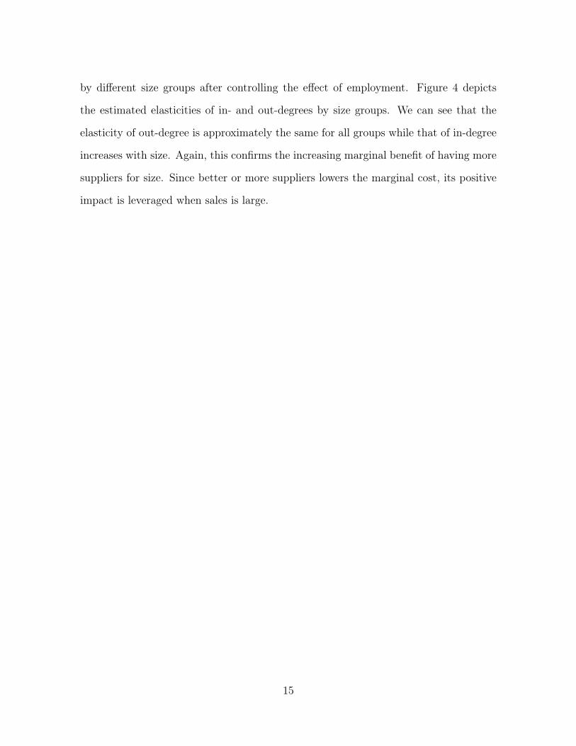
Table 2 presents the estimated coefficients with firm fixed effects. All the qualitative

features are the same as the case of no firm fixed effects. Hence, the results are not

driven by the heterogeneity across firms, and hold for change to change over firm life

cycle. The first three columns show that the growth of in- and out-degrees are positively

associated with sales growth. Again, the coefficient is larger for in-degree. The last three

columns also confirm the robustness of the positive impact of the customer and supplier

sets, and the complementarity between in- and out-degrees.

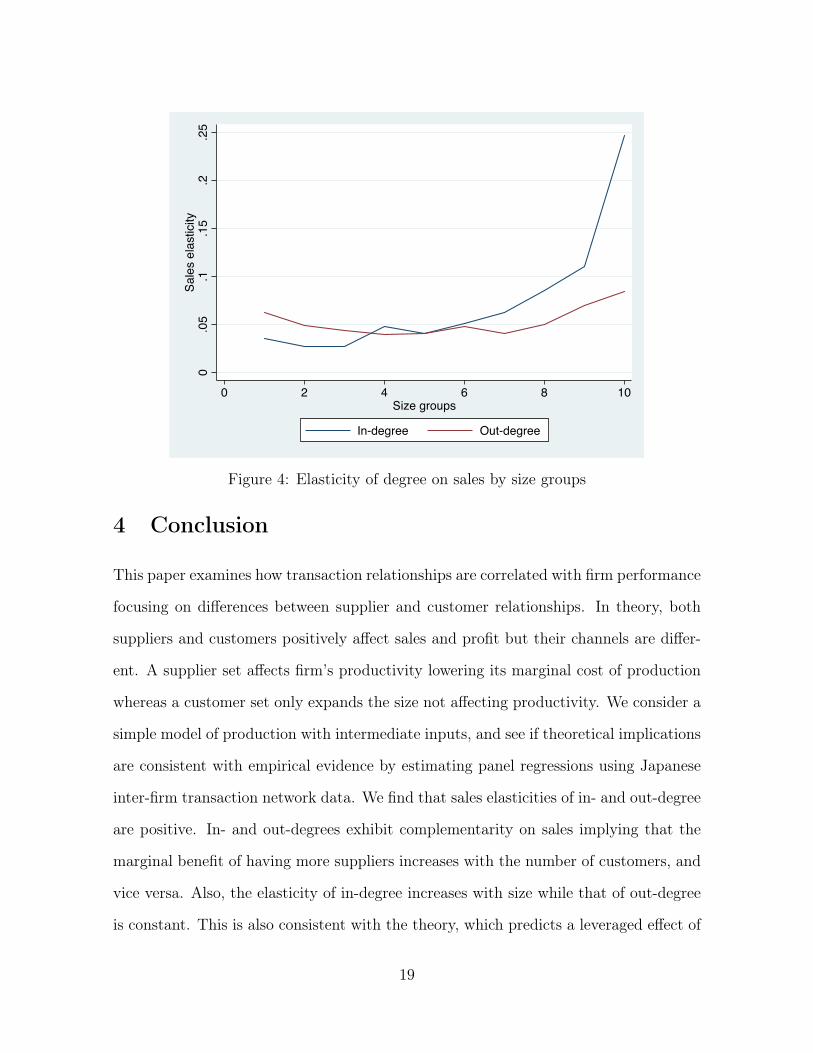
To see the difference in sales elasticities across size groups, we divided firms into ten

groups based on their mean sales across time. Table 3 presents the elasticities on sales

14

by different size groups after controlling the effect of employment. Figure 4 depicts

the estimated elasticities of in- and out-degrees by size groups. We can see that the

elasticity of out-degree is approximately the same for all groups while that of in-degree

increases with size. Again, this confirms the increasing marginal benefit of having more

suppliers for size. Since better or more suppliers lowers the marginal cost, its positive

impact is leveraged when sales is large.

15

(1) (2) (3) (4) (5) (6) (7) (8)Sales Sales Sales Sales Sales Sales Sales Sales

In-degree 1.118*** 0.871*** 0.881*** 0.747*** 0.761*** 0.611*** 0.630***(0.000556) (0.000746) (0.00348) (0.00108) (0.00379) (0.00190) (0.00528)

Out-degree 0.927*** 0.433*** 0.429*** 0.299*** 0.299*** 0.304*** 0.300***(0.000638) (0.000730) (0.00287) (0.00106) (0.00275) (0.00172) (0.00384)

Ratio of new in-degree 0.350*** 0.348*** 0.332***(0.0649) (0.0646) (0.0631)

Ratio of new out-degree 0.156*** 0.151*** 0.136***(0.0105) (0.0105) (0.0104)

In-degree × out-degree 0.0788*** 0.0764*** 0.0754*** 0.0717***(0.000459) (0.000511) (0.000508) (0.000583)

In-degree × age 0.00328*** 0.00321***(4.23e-05) (5.56e-05)

Out-degree × age -0.000969*** -0.000794***(4.09e-05) (5.36e-05)

Constant 10.94*** 10.92*** 10.91*** 10.83*** 11.04*** 10.96*** 11.18*** 11.10***(0.00630) (0.00661) (0.00704) (0.0121) (0.00704) (0.0123) (0.00719) (0.0128)

Observations 7,191,843 6,512,372 4,930,832 4,418,792 4,930,832 4,418,792 4,695,762 4,209,399R-squared 0.453 0.390 0.531 0.540 0.534 0.544 0.528 0.537

Table 1: Panel regression results (without firm fixed effects)

16

(1) (2) (3) (4) (5) (6)Sales Sales Sales Sales Sales Sales

In-degree 0.158*** 0.146*** 0.156*** 0.0922*** 0.105***(0.000480) (0.000564) (0.000646) (0.000758) (0.000839)

Out-degree 0.101*** 0.0796*** 0.0889*** 0.0272*** 0.0392***(0.000433) (0.000493) (0.000579) (0.000695) (0.000779)

Ratio of new in-degree 0.0323*** 0.0323***(0.000426) (0.000426)

Ratio of new out-degree 0.0229*** 0.0225***(0.000411) (0.000410)

In-degree × out-degree 0.0435*** 0.0413***(0.000407) (0.000434)

In-degree × age

Out-degree × age

Constant 12.01*** 11.98*** 12.17*** 12.14*** 12.22*** 12.18***(0.000626) (0.000627) (0.000908) (0.00105) (0.001000) (0.00114)

Observations 7,191,843 6,512,372 4,930,832 4,418,792 4,930,832 4,418,792R-squared 0.968 0.968 0.971 0.973 0.971 0.973

Table 2: Panel regression results (with firm fixed effects)

17

(1) (2) (3) (4) (5) (6) (7) (8) (9) (10)Group 1 Group 2 Group 3 Group 4 Group 5 Group 6 Group 7 Group 8 Group 9 Group 10

In-degree 0.0359 0.0268 0.0276 0.0482 0.0407 0.0513 0.0624 0.0857 0.110 0.247(0.00471) (0.00352) (0.00316) (0.00307) (0.00284) (0.00280) (0.00287) (0.00296) (0.00329) (0.00432)

Out-degree 0.0625 0.0489 0.0437 0.0392 0.0408 0.0480 0.0407 0.0496 0.0694 0.0846(0.00406) (0.00320) (0.00297) (0.00295) (0.00279) (0.00283) (0.00292) (0.00297) (0.00322) (0.00371)

Employment 0.316 0.333 0.340 0.352 0.350 0.367 0.379 0.356 0.382 0.406(0.00444) (0.00364) (0.00349) (0.00356) (0.00349) (0.00336) (0.00356) (0.00339) (0.00346) (0.00369)

Constant 9.919 10.57 10.90 11.13 11.39 11.59 11.82 12.18 12.47 12.95(0.00672) (0.00719) (0.00789) (0.00894) (0.00955) (0.0101) (0.0117) (0.0125) (0.0146) (0.0203)

Observations 112,600 112,587 112,704 112,467 112,576 112,585 112,587 112,587 112,586 112,577R-squared 0.839 0.526 0.450 0.421 0.399 0.400 0.416 0.481 0.652 0.961

Table 3: Results by different size groups

18

0.0

5.1

.15

.2.2

5Sa

les

elas

ticity

0 2 4 6 8 10Size groups

In-degree Out-degree

Figure 4: Elasticity of degree on sales by size groups

4 Conclusion

This paper examines how transaction relationships are correlated with firm performance

focusing on differences between supplier and customer relationships. In theory, both

suppliers and customers positively affect sales and profit but their channels are differ-

ent. A supplier set affects firm’s productivity lowering its marginal cost of production

whereas a customer set only expands the size not affecting productivity. We consider a

simple model of production with intermediate inputs, and see if theoretical implications

are consistent with empirical evidence by estimating panel regressions using Japanese

inter-firm transaction network data. We find that sales elasticities of in- and out-degree

are positive. In- and out-degrees exhibit complementarity on sales implying that the

marginal benefit of having more suppliers increases with the number of customers, and

vice versa. Also, the elasticity of in-degree increases with size while that of out-degree

is constant. This is also consistent with the theory, which predicts a leveraged effect of

19

lowering a marginal cost when the scale is large.

20

References

Antras, Pol, Teresa C. Fort, and Felix Tintelnot (2017) “The Margins of Global Sourcing:

Theory and Evidence from US Firms,” American Economic Review, Vol. 107, No.

9, pp. 2514–64.

Baqaee, David Rezza (2017) “Cascading Failures in Production Networks,” Working

Paper.

Bernard, Andrew B., Andreas Moxnes, and Yukiko U. Saito (2015) “Production Net-

works, Geography and Firm Performance,” NBER Working Paper 21082.

Carvalho, Vasco M., Makoto Nirei, and Yukiko U. Saito (2014) “Supply Chain Dis-

ruptions: Evidence frmo the Great East Japan Earthquake,” RIETI Discussion

Paper Series 14-E-035.

Fujii, Daisuke (2016) “Shock Propagations in Granular Networks,” RIETI Discussion

Paper Series 16-E-057.

Lim, Kevin (2017) “Frim-to-firm Trade in Sticky Production Networks,” Working Paper.

Saito, Yukiko U., Tsutomu Watanabe, and Mitsuru Iwamura (2007) “Do Larger Firms

Have More Interfirm Relationship?” RIETI Discussion Paper Series 07-E-028.

21