FIRING RATE ANALYSIS FOR A LINEAR

INTEGRATE-AND-FIRE NEURONAL MODEL

by

Ryan M. O’Grady

B.S., Allegheny College, 2002

M.A., University of Pittsburgh, 2009

Submitted to the Graduate Faculty of

the Department of Mathematics in partial fulfillment

of the requirements for the degree of

Doctor of Philosophy

University of Pittsburgh

2011

UNIVERSITY OF PITTSBURGH

MATHEMATICS DEPARTMENT

This dissertation was presented

by

Ryan M. O’Grady

It was defended on

April 22, 2011

and approved by

William C. Troy, Department of Mathematics

Brent Doiron, Department of Mathematics

Gunduz Caginalp, Department of Mathematics

Satish Iyengar, Department of Statistics

Dissertation Director: William C. Troy, Department of Mathematics

ii

FIRING RATE ANALYSIS FOR A LINEAR INTEGRATE-AND-FIRE

NEURONAL MODEL

Ryan M. O’Grady, PhD

University of Pittsburgh, 2011

We investigate a stochastic linear integrate-and-fire (IF) neuronal model and use the corre-

sponding Fokker-Planck equation (FPE) to study the mean firing rate of a population of IF

neurons. The firing rate (or emission rate) function, ν(t), is given in terms of an eigenfunc-

tion expansion solution of the FPE. We consider two parameter regimes of current input and

prove the existence of infinitely many branches of eigenvalues and derive their asymptotic

properties. We use the eigenfunction expansion solution to prove asymptotic properties of

the firing rate function, ν(t). We also perform a numerical experiment of 10, 000 IF neurons

and show that our simulation is in agreement with our theoretical results. Finally, we state

several open problems for future research.

iii

TABLE OF CONTENTS

PREFACE . . . . . . . . . . . . . . . . . . . . . . . . . . . . . . . . . . . . . . . . . x

1.0 INTRODUCTION . . . . . . . . . . . . . . . . . . . . . . . . . . . . . . . . . 1

1.1 The Mean Firing Rate in Neurons . . . . . . . . . . . . . . . . . . . . . . . 1

1.2 Mathematical Models . . . . . . . . . . . . . . . . . . . . . . . . . . . . . . 2

1.2.1 The Integrate-and-Fire Model . . . . . . . . . . . . . . . . . . . . . . 3

1.2.2 The Leaky Integrate-and-Fire Model . . . . . . . . . . . . . . . . . . 3

1.2.3 The Hodgkin-Huxley Equations: The Space Clamped Simplification . 4

1.2.4 Simplifications of the Hodgkin-Huxley Equations . . . . . . . . . . . 4

1.3 Stochastic Integrate-and-Fire Models . . . . . . . . . . . . . . . . . . . . . 5

1.3.1 Why study integrate-and-fire models rather than HH type models . . 6

1.4 The Focus of This Thesis . . . . . . . . . . . . . . . . . . . . . . . . . . . . 11

1.5 Our Mathematical Results . . . . . . . . . . . . . . . . . . . . . . . . . . . 13

1.5.1 Thesis Goals and Results . . . . . . . . . . . . . . . . . . . . . . . . 13

1.5.2 Chapter Outline . . . . . . . . . . . . . . . . . . . . . . . . . . . . . 14

2.0 LEAKY (LIF) AND LINEAR (IF) MODELS: A COMPARISON . . . 17

2.1 The Leaky Integrate-and-Fire Model . . . . . . . . . . . . . . . . . . . . . . 18

2.1.1 The Fokker-Plank Equation FPE for the LIF Model . . . . . . . . . 18

2.1.2 The Firing Rate Function for the LIF Model . . . . . . . . . . . . . . 19

2.1.3 The FPE BVP for the LIF Model . . . . . . . . . . . . . . . . . . . . 20

2.2 The Linear Integrate-and-Fire Model . . . . . . . . . . . . . . . . . . . . . 20

2.2.1 The Fokker-Plank Equation for the IF Model . . . . . . . . . . . . . 21

2.2.2 The Firing Rate Function for the IF Model . . . . . . . . . . . . . . 22

iv

2.2.3 The FPE Boundary Value Problem for the IF Model . . . . . . . . . 22

2.3 Eigenfunction Expansion for the LIF Model . . . . . . . . . . . . . . . . . . 23

2.3.1 The ODE BVP for Eigenfunctions of the LIF Model . . . . . . . . . 24

2.3.2 Stationary Solution of the FPE of the LIF Model . . . . . . . . . . . 25

2.3.3 Behavior of the Stationary Solution of the LIF . . . . . . . . . . . . 29

2.3.4 Numerical Exploration of the Neighborhood U . . . . . . . . . . . . 33

2.3.5 The Difficulty in the LIF Eigenvalue Problem . . . . . . . . . . . . . 34

2.4 The Eigenfunction Expansion for the IF Model . . . . . . . . . . . . . . . . 34

2.4.1 The ODE BVP for Eigenfunctions of the IF Model . . . . . . . . . . 36

2.4.2 ODE Eigenvalue Problem for the Case VL = VR . . . . . . . . . . . . 37

2.4.3 The Eigenvalue Problem for the IF in the General Case . . . . . . . 42

2.4.4 The Stationary Solution when VL = −∞ . . . . . . . . . . . . . . . . 47

2.5 Conclusion and Open Problem . . . . . . . . . . . . . . . . . . . . . . . . . 49

3.0 BACKGROUND PROPERTIES OF THE IF MODEL WHEN VL = VR 50

3.1 The Linear Integrate and Fire (IF) FPE Boundary Value Problem . . . . . 51

3.2 The Operators L and L+ when VL = VR = 0. . . . . . . . . . . . . . . . . . 55

3.3 The Eigenfunction Expansion When VL = VR . . . . . . . . . . . . . . . . . 57

3.4 The Mattia-Del Giudice Conjecture . . . . . . . . . . . . . . . . . . . . . . 58

4.0 THE MAIN RESULTS: EXISTENCE OF EIGENVALUES WHEN

VL = VR . . . . . . . . . . . . . . . . . . . . . . . . . . . . . . . . . . . . . . . . 59

4.1 Eigenvalue Structure of the IF When VL = VR . . . . . . . . . . . . . . . . 60

4.1.1 The Fokker Planck Problem When −∞ < VL = VR < θ . . . . . . . . 60

4.1.2 The Eigenvalue Problem When VL = VR . . . . . . . . . . . . . . . . 61

4.1.3 The Nonlinear Eigenvalue Equation . . . . . . . . . . . . . . . . . . . 62

4.1.4 The Eigenfunctions φn of L and ψn of L+ . . . . . . . . . . . . . . . 64

4.2 Eigenvalues for the IF model when µ = 0 . . . . . . . . . . . . . . . . . . . 66

4.2.1 The ODE Boundary Value Problem . . . . . . . . . . . . . . . . . . 66

4.2.2 The Main Theoretical Result . . . . . . . . . . . . . . . . . . . . . . 67

4.3 Eigenvalues for the IF model when z = µθσ2 > 0 . . . . . . . . . . . . . . . . 77

4.3.1 The Nonlinear Algebraic Equations for γ1 and γ2 . . . . . . . . . . . 78

v

4.3.2 ODEs for γ1 and γ2 . . . . . . . . . . . . . . . . . . . . . . . . . . . 79

4.3.3 Infinitely Many Initial Values for the (γ1, γ2) ODEs. . . . . . . . . . 80

4.3.3.1 Outline of the Proof of Theorem 3 . . . . . . . . . . . . . . . 81

4.3.3.2 Proof of Theorem 3. . . . . . . . . . . . . . . . . . . . . . . . 81

4.3.4 Infinitely many C1((0,∞)) solutions of the ODEs. . . . . . . . . . . 93

4.3.5 Properties of λn1 (z) and λn2 (z) as z = µθσ2 → 0+ . . . . . . . . . . . . . 106

4.4 Eigenvalues for the IF model when z = µθσ2 < 0 . . . . . . . . . . . . . . . . 110

4.4.1 Existence and Asymptotic Behavior When z = µθσ2 < 0 . . . . . . . . 111

4.4.1.1 Proof of Theorem 8. . . . . . . . . . . . . . . . . . . . . . . . 113

4.4.1.2 Proof of Theorem 9. . . . . . . . . . . . . . . . . . . . . . . . 116

4.4.1.3 Proof of Theorem 10. . . . . . . . . . . . . . . . . . . . . . . 129

4.4.1.4 Proof of Theorem 11. . . . . . . . . . . . . . . . . . . . . . . 132

4.5 Partial Proof of the Mattia-Del Giudice Conjecture when µ > 0 . . . . . . . 135

4.5.1 All Eigenvalues are Complex When µ > 0 . . . . . . . . . . . . . . . 136

4.5.2 The Real Parts of the Eigenvalues are Negative . . . . . . . . . . . . 142

4.5.3 Open Problem: Real parts of the Eigenvalues are Negative . . . . . . 143

4.6 Partial Proof of the Mattia-Del Giudice Conjecture when µ < 0 . . . . . . . 144

4.6.1 Eigenvalues are Negative when γ1 = 0 . . . . . . . . . . . . . . . . . 144

4.6.2 Open Problem: The Eigenvalues are Real and Negative . . . . . . . . 145

5.0 THE FIRING RATE . . . . . . . . . . . . . . . . . . . . . . . . . . . . . . . 146

5.1 Numerical Simulations for IF when µ > 0 . . . . . . . . . . . . . . . . . . . 146

5.1.1 Numerical Computation of the Eigenvalues. . . . . . . . . . . . . . . 147

5.1.1.1 Remarks About the Eigenvalue Tables . . . . . . . . . . . . . 148

5.1.2 The Firing Rate Function . . . . . . . . . . . . . . . . . . . . . . . . 149

5.1.2.1 Numerical Simulation of a Population of IF neurons . . . . . 149

5.2 Firing Rate Analysis when µ > 0 . . . . . . . . . . . . . . . . . . . . . . . . 150

5.2.1 The Firing Rate function generated by the FPE. . . . . . . . . . . . 150

5.2.2 Asymptotic Results for the Firing Rate Function . . . . . . . . . . . 152

5.2.3 Relative Error Between Theoretical and Numerical Values of ν(∞) . 153

5.3 Firing Rate when µ(t) is a step function . . . . . . . . . . . . . . . . . . . . 153

vi

5.3.1 Theoretical Firing rate . . . . . . . . . . . . . . . . . . . . . . . . . . 154

5.3.2 Population Firng Rate . . . . . . . . . . . . . . . . . . . . . . . . . . 155

5.4 Proof that E([νN(t)− ν(t)]2

)≈ ν(t)

N∆t, N >> 1. . . . . . . . . . . . . . . . 156

6.0 OPEN PROBLEMS AND FUTURE RESEARCH . . . . . . . . . . . . . 170

6.1 Open Problem 1: Extremum properties of the Stationary Solution for the

LIF FPE . . . . . . . . . . . . . . . . . . . . . . . . . . . . . . . . . . . . . 170

6.2 Open Problem 2: Existence of eigenvalues and eigenfunctions for the LIF FPE171

6.3 Open Problem 3: Resolution of the Mattia-Del Giudice Conjecture for the

IF Model . . . . . . . . . . . . . . . . . . . . . . . . . . . . . . . . . . . . . 171

APPENDIX. NUMERICAL CODES . . . . . . . . . . . . . . . . . . . . . . . . 173

A.1 Reproducing the plots of the stationary solutions for the LIF and IF . . . . 173

A.2 Numerical Investigation of the Neighborhood U . . . . . . . . . . . . . . . . 180

A.3 The functions γ(z) and λ(z) . . . . . . . . . . . . . . . . . . . . . . . . . . 181

A.4 Calculating the Eigenvalues for the FPE of the IF model . . . . . . . . . . 188

A.5 The Firing Rate Function . . . . . . . . . . . . . . . . . . . . . . . . . . . . 190

A.5.1 Calculating the Theoretical Firing Rate, ν(t) . . . . . . . . . . . . . 190

A.5.2 Simulation of the Population Firing Rate . . . . . . . . . . . . . . . 193

BIBLIOGRAPHY . . . . . . . . . . . . . . . . . . . . . . . . . . . . . . . . . . . . 197

vii

LIST OF TABLES

1 Gamma Values when µ = 20 . . . . . . . . . . . . . . . . . . . . . . . . . . . 158

2 Eigenvalues when µ = 20 . . . . . . . . . . . . . . . . . . . . . . . . . . . . . 159

3 Gamma Values when µ = 5 . . . . . . . . . . . . . . . . . . . . . . . . . . . . 160

4 Eigenvalues when µ = 5 . . . . . . . . . . . . . . . . . . . . . . . . . . . . . . 161

5 Gamma Values when µ = 1 . . . . . . . . . . . . . . . . . . . . . . . . . . . . 162

6 Eigenvalues when µ = 1 . . . . . . . . . . . . . . . . . . . . . . . . . . . . . . 163

7 Gamma Values when µ = 0.1 . . . . . . . . . . . . . . . . . . . . . . . . . . . 164

8 Eigenvalues when µ = 0.1 . . . . . . . . . . . . . . . . . . . . . . . . . . . . . 165

9 Relative Error . . . . . . . . . . . . . . . . . . . . . . . . . . . . . . . . . . . 169

viii

LIST OF FIGURES

1 The firing rate when µ(t) is a step function . . . . . . . . . . . . . . . . . . . 10

2 Stationary solution of the LIF when τ = 1 . . . . . . . . . . . . . . . . . . . . 27

3 Stationary solution of the LIF when τ = 20 . . . . . . . . . . . . . . . . . . . 28

4 The neighborhood U . . . . . . . . . . . . . . . . . . . . . . . . . . . . . . . . 35

5 Stationary solution of the IF when VL = VR . . . . . . . . . . . . . . . . . . . 41

6 Stationary solution of the IF when VL < VR . . . . . . . . . . . . . . . . . . . 48

7 The rectangle Bn . . . . . . . . . . . . . . . . . . . . . . . . . . . . . . . . . . 82

8 The rectangle Dn and the initial point for the ODE . . . . . . . . . . . . . . 95

9 The functions γ1(z) and γ2(z) . . . . . . . . . . . . . . . . . . . . . . . . . . . 96

10 The eigenvalues λ1(z) and λ2(z) . . . . . . . . . . . . . . . . . . . . . . . . . 107

11 γ1(z), γ2(z) and corresponding eigenvalues for µ < 0. . . . . . . . . . . . . . . 114

12 Theoretical Firing Rate . . . . . . . . . . . . . . . . . . . . . . . . . . . . . . 166

13 Firing Rate: Population versus Theoretical . . . . . . . . . . . . . . . . . . . 167

14 Firing Rate as µ varies . . . . . . . . . . . . . . . . . . . . . . . . . . . . . . 168

15 The firing rate when µ(t) is a step function . . . . . . . . . . . . . . . . . . . 169

ix

PREFACE

The completion of this thesis would not have been possible without the assistance and

support of several people.

Most importantly, I would like to thank my advisor Professor William C. Troy. His

insight, guidance, and patience are truly invaluable.

To my committee members, Professors Brent Doiron, Gunduz Caginalp, and Satish Iyen-

gar: thank you for being excellent teachers and mentors. Your courses and personal discus-

sions have been helpful and productive.

I would also like to thank Dr. Cheng Ly, Dr. Mark DeSantis, Sashi Marella, and Justin

Dunmyre. Each of you has been a great help over the last few years. Your insight and

suggestions were greatly appreciated.

The Pitt math department faculty, staff, and students: you have all made the last few

years challenging and exciting. Thank you!

Lastly, I must thank my family and friends, especially Amy. You have know clue what it

is that I do, yet you only complain some of the time. I wish this thesis could serve as proof

that I have actually worked over the last few years. However, I am quite sure you won’t

understand a word that follows this!

x

1.0 INTRODUCTION

The purpose of this thesis is to provide mathematical analysis of the firing rate of a linear

integrate-and-fire neuronal model (1.10). In this chapter we introduce the notion of mean

firing rate of a neuron, its importance, and how it is studied mathematically. Next, goals

and mathematical results are discussed. In particular, we do the following:

1.1 This section gives a motivation of the main problem in this thesis: mean firing rate

analysis of a neuron.

1.2 This section gives a description of the important mathematical models used to study the

mean firing rate over the last 104 years.

1.3 This section introduces the two stochastic integrate-and-fire neuronal models analyzed

in this thesis. We describe the advantages and disadvantages of studying these models.

1.5 This section describes our main mathematical results. An outline is given which describes

the results proved in each chapter.

1.1 THE MEAN FIRING RATE IN NEURONS

The concept of mean firing rate in neurons has been a central focus of experimental studies

ever since the pioneering work of Adrian and Zotterman [1, 2] in 1926. These authors gave

evidence which showed how frog muscle responded to stimulation of single motor neuron

nerve fibers. The stimulation they used included the pressure on the muscle, as well as

pricking the muscle with a needle. Their recordings “showed that the firing rate of stretch

receptor neurons in the muscles is related to the force applied to the muscle” (Gerstner and

1

Kistler [13]). In 1928 Adrian and Bronk [3] extended the experimental techniques in [1, 2]

to record the firing rate response of skin to a stimulus of constant intensity. Due to the

ease of measuring firing rates experimentally, this method has been widely used over the last

83 years [13]. As pointed out by Gerstner and Kistler in their 2002 textbook [13], a central

modern day issue is to understand the role of mean firing rate in the mammalian brain, which

“contains more than 1010 densely packed neurons that are connected to an intricate network.

In every small volume of cortex, thousands of spikes are emitted each millisecond.” These

large scale neuronal firing properties have led to the following fundamental questions (e.g.

see Gerstner and Kistler [13], Haken [14], Tuckwell [35]):

• Question 1. What is the information contained in a spatio-temporal pattern of pulses?

• Question 2. What is the code used by the neurons to transmit the information in a

spatio-temporal pattern of pulses?

• Question 3. How might other neurons decode the signal?

• Question 4. As external observers, can we read the code and understand the message

of the neuronal activity pattern?

An important approach to answering Questions 1-4 is to investigate firing rate phenomena

in mathematical models. Below, we describe relevant models.

1.2 MATHEMATICAL MODELS

A first step in addressing the issues raised in Questions 1-4 above is to combine exper-

imental results, together with mathematical modeling, in order to understand underlying

mechanisms responsible for firing rate phenomena in neuronal settings. Thus, in this section

our goal is to give a brief description of mathematical models that have been used during

the last 100 years to understand firing rate phenomena.

2

1.2.1 The Integrate-and-Fire Model

One of the earliest models (e.g. see Tuckwell [35], Cronin [8]) of neuronal firing is the equation

CmdVmdt

= I(t), (1.1)

where Vm(t) and I(t) are the transmembrane voltage and current, respectively. This model,

which was proposed in 1907 by Louis Lapicque [21], results from taking the time derivative

of the law of capacitance CmVm(t) = Q(t). When a positive constant current I is applied in

equation (1.1), the membrane voltage increases with time until Vm(tT ) = threshold = VT at

a time tT . At tT a delta function spike occurs and the voltage Vm(t) is reset to its resting

potential, V = VR < VT , after which the model again determines the behavior of Vm(t). As

the input current I(t) is increased the firing frequency of the neuron also increases. One way

to improve the biological accuracy of this model is to introduce a refractory period TR > 0,

which limits the frequency of firing during a period of length TR immediately following the

voltage reset after the neuron fires[35]. Thus, when TR > 0, the maximum firing frequency of

the neuron is 1/TR. In a recent review article by Brunel and Van Rossum [6], they point out

that “the simplicity of equation (1.1) makes it one of the most popular models of neuronal

firing to this day: it has been used in computational neuroscience for both cellular and neural

networks studies, as well as in mathematical neuroscience.”

1.2.2 The Leaky Integrate-and-Fire Model

A more biologically accurate model is the leaky integrate-and-fire model (e.g. see [35]) given

by the equation

CmdVmdt

+Vm(t)

Rm

= I(t). (1.2)

Rm is the membrane resistance. As with the integrate-and-fire model (1.1), the membrane

voltage increases with time until Vm(tT ) = threshold = VT at a time tT . At tT a delta function

spike occurs and the voltage Vm(t) is reset to its resting potential, V = VR, after which the

model (1.2) again determines the behavior of Vm(t).

3

1.2.3 The Hodgkin-Huxley Equations: The Space Clamped Simplification

In 1952 Hodgkin and Huxley [16] introduced the following nonlinear system to model a space

clamped axon:

dV

dt=

1

CM

[I − gNam3h (V − VNa)− gKn4 (V − VK)− gl (V − Vl)

],

dm

dt= αm (1−m)− βmm,

dh

dt= αh (1− h)− βhh,

dn

dt= αn (1− n)− βnn.

Here, V is membrane potential, and the variables m, n, and h where proposed by Hodgkin

and Huxley to control the conductance of sodium and potassium ions. The functions αm,

βm, αh, βh, αn, βn in the odes for m, n, and h are assumed to be functions of V. The

Hodgkin-Huxley (HH) equations model the variations of the membrane potential and ion

conductance that occur at a fixed point of the neuron [8]. The difficulty in analytically

studying neuronal mean firing rate in the HH system is that the functions αm, βm, αh, βh,

αn, βn are transcendental [14]. Also, experimental indicates that the threshold is not well

defined, hence the maximum voltage varies during a spike [17].

1.2.4 Simplifications of the Hodgkin-Huxley Equations

The FitzHugh-Nagumo Model

To aid in the study of the HH equations, simplifications have been made [8, 14, 35]. A

fundamentally important example is the two-dimensional model developed independently

by Fitzhugh [10] and Nagumo [26] given by the system

dV

dt= V − 1

3V 3 −W + I,

dW

dt= φ (V + a− bW ) ,

where a, b, and φ are positive constants. As before, I is the membrane current and V is the

membrane potential. The new function W is a recovery variable.

4

The Morris-Lecar Equations

In 1981 Morris and Lecar combined Hodgkin-Huxley and FitzHugh-Nagumo into a voltage-

gated calcium channel model with a delayed-rectifier potassium channel, represented by

CdV

dt= −Iion(V,w) + I

dw

dt= φ

w∞ − wτw(V )

where

Iion(V,w) = gCam∞(V )(V − VCa) + gKw(V − VK) + gL(V − VL).

Other two variable models similar to the FitzHugh-Nagumo equations, and the Morris-

Lecar system, have been developed by Hindmarsh-Rose [15] in 1984, Rinzel [29] in 1985 and

Wilson [36] in 1999.

1.3 STOCHASTIC INTEGRATE-AND-FIRE MODELS

As Tuckwell [35] points out (see page 111 in Vol II), the deterministic models discussed in Sec-

tion 1.2 are inadequate when describing firing rate behavior (and hence address Questions

1-4) for a real neuron. In particular, sequences of firing times in experimentally studied

neurons are random. This is due to thermo-molecular processes and channel noise. The

overwhelming source of randomness is from synaptic transmission (e.g. the random arrival

of synaptic events, and/or synaptic failure). This randomness in firing rate characterizes the

behavior of realistic neurons, hence realistic models should be stochastic. Stochastic firing

rate models where first introduced by Gerstein and Mandelbrot [12] in 1964, and subsequently

by Stein [32] in 1965, and Knight [18] in 1972. Fusi and Mattia [11] introduced refractory

barriers in stochastic integrate-and-fire models in 1999. Two of the most widely studied

stochastic integrate-and-fire models are known as leaky integrate-and-fire (LIF) model and

the linear integrate-and-fire (IF) model. These models, which are the focus of this thesis,

are extensions of equations (1.1) and (1.2), and are described below:

5

I. The stochastic linear integrate-and-fire (IF) model, which is an extension of (1.1) consists

of the stochastic differential equation (SDE)

dV = µ(t)dt+ σ(t)dW. (1.3)

Here, the membrane potential V (t) satisfies V ∈ [VL, VT ], where VL ≤ VR < VT , σ(t)dW rep-

resents Brownian motion, and the function µ(t) describes the input of current. The param-

eter VL represents the lowest possible value of transmembrane potential. For a real neuron,

VL ≈ −85 mV, which corresponds to the reversal potential for potassium (see Section 2.2 for

further discussion). Descriptions of this model, together with the eigenfunction-eigenvalue

expansion approach to its analysis, were given by Knight [18, 19] in 1972 and 2000, and by

Mattia and Del Giudice [24] in 2002.

II. The stochastic leaky integrate-and-fire (LIF) model, which is an extension of (1.2) consists

of the SDE

dV =

(µ(t)− V

τ

)dt+ σ(t)dW, (1.4)

where −Vτ

is a leakage term that is not present in the IF model (1.3). A complete description

of this spiking model is given by Gerstner and Kistler [13].

1.3.1 Why study integrate-and-fire models rather than HH type models

As pointed out by Tuckwell [35], Cronin [8], Lindner [22] and Izhikevich [17], integrate-and-

fire models are not as biologically accurate as conductance based HH type models described

above in Section 1.2. The obvious question arises: why study integrate-and-fire models rather

than HH type models? Three important reasons for studying integrate-and-fire models are

the following:

I. Computational efficiency. In 2004 Izikevich [17] published the paper “Which Model to

Use for Cortical Spiking Neurons?” in which compared the efficiency and accuracy of firing

rates in a multitude of diverse models. These include integrate-and-fire models, the Hodgkin

Huxley equations, the FitzHugh-Nagumo system, and the Morris-Lecar model. He found

that integrate-and-fire models were computationally very efficient, whereas Hodgkin-Huxley

6

type systems were extremely inefficient, for recording firing rates in populations of large

numbers of neurons. For example, a 1ms simulation of an IF model requires approximately

5 flops1 while a Hodgkin-Huxley simulation for 1ms requires approximately 1200 flops.

II. Applicability. Below, we describe five examples of recent studies which have successfully

made use of integrate-and-fire models to understand firing rate phenomena in biological

systems.

(A.) In 2006 Doiron, Rinzel and Reyes used a multi-layer IF model to show that interaction

between populations of spiking neurons in the cortex may depend critically on the size of the

populations. In particular, they performed a simulation of 10 layers of 500 IF neurons. Their

results agreed with experimentally observed behavior in a rat somatosensory cortex [28].

(B.) In 2008, Mullowney and Iyengar [25] studied maximum likelihood estimates of a leaky

integrate-and-fire neuron. They develop an algorithm for estimating parameters when only

the firing rate is known. Their results were in agreement with previously published theoretical

results.

(C.) In 2009 Ly and Doiron [23] used integrate-and-fire models to successfully estimate

dynamic neural response in normal sensory and motor behavior. In particular, they con-

struct an integrate-and-fire model with realistic, time varying inputs that agree with clamp

experimental data in rat somatosensory cortex [7].

(D.) In 2009, Okamoto and Fukai [27] make use of integrate-and-fire model to study neu-

ronal firing rate behavior in rat prefrontal and entorhinal cortex. Their results suggest that

populations of neurons (in various brain areas) can act like non-leaky integrate-and-fire neu-

rons at the population level. In addition, their results are in agreement with in agreement

with experimental observations.

(E.) In his 2011 PH.D. thesis, Sashi Morelli [] obtained theoretical predictions of the firing

rate of IF and LIF model neurons receiving mean or variance coded time-varying inputs.

These predictions were tested via real neurons in the somatosensory cortex of a rat.

III. Mathematical tractability. Because of the simplicity of stochastic integrate-and-

1The number of flops represents the number of floating point operations required for a simulation

7

fire models, they are much easier to analyze than systems of nonlinear HH conductance

type models which have large numbers of functions and constants. To study stochastic

integrate-and-fire type models, Knight [18, 19], as well as Mattia and Del Giudice [24], have

successfully made use of eigenfunction expansion methods to study solutions of the Fokker

Planck Equation (FPE) corresponding to the IF SDE (1.3):

∂

∂tρ = −µ(t)

∂

∂Vρ+

σ2(t)

2

∂2

∂V 2ρ+ ν(t)δ(V − VR), (1.5)

where V (t) ∈ [VL, VT ], and V (t) satisfies a reflective boundary condition at VL. An eigen-

function expansion solution of the FPE1.5, which has the form

ρ(V, t|V0, 0) =∑λ

An(t)eλtφn(V ), (1.6)

has allowed these authors to successfully investigate the behavior of the firing rate (or emis-

sion rate) function

ν(t) = −σ2

2

∂

∂Vρ(VT , t|V0, 0). (1.7)

Question: What is the connection between the mean firing rate of a population

of real neurons and the mean firing rate constructed by using the eigenfunction

expansion method?

In real nervous systems neurons react to inputs from dynamic environments (e.g. sensory,

memory recall). The input statistics for a given neuron change during the course of a task.

Thus, in the context of the stochastic IF SDE equation (1.3), µ(t) and/or σ(t) are time

dependent quantities. A simple example illustrating this property is when the neuron input

µ(t) is a step function, e.g.

µ(t) =

0 0 ≤ t < T ∗ = 1000 msec.,

25 t ≥ T ∗,

(1.8)

and σ(t) is constant, e.g.

σ(t) = 1 ∀t ≥ 0. (1.9)

The left panel of Figure 1 illustrates a simulation of population mean firing rate, νN(t),

for N = 10, 000 neurons. Here, we assume that each neuron satisfies the initial condition

8

V (0) = VR = 0. Over the subinterval 0 ≤ t < T ∗ = 1000 the neurons receive constant

input µ = 0, and the population mean firing rate quickly relaxes to the equilibrium level

νN(∞) ≈ 1. When t ≥ 1000 the input discontinuously jumps to the new constant level

µ = 25. In response to this discontinuous change of input, the population mean firing rate

initially undergoes oscillations (i.e. ringing) with peaks that decrease in amplitude during a

transition period of length approximately 200 msecs. By the end of this transition interval,

the firing rate has relaxed to its equilibrium level, νN ≈ 25. The right panel shows the

theoretical mean firing rate, ν(t), resulting from the eigenfunction expansion method. During

the transition interval, [1000, 1200), the theoretical firing rate ν(t) also undergoes oscillations,

with peaks that decrease to zero in amplitude as the ν(t) relaxes to its equilibrium level,

ν ≈ 25 (see Section 5.2.2). A major thrust of this thesis is to give a firm foundation to

the use of the eigenfunction expansion to understand non equilibrium behavior of firing

rate when µ and σ are constant during the two subintervals [0, T ∗) and [T ∗,∞). Our study

includes the parameter regime µ > 0 and σ > 0, and also the regime µ < 0 and σ > 0.

Eigenfunction expansions have played an important rule in several of the neuronal studies

described above ( e.g. studies (A), (C) and (E)). In each application, numerical simulations

led the authors to assume, without proof, that branches of eigenvalues, and corresponding

eigenfunctions actually exist. However, to our knowledge there has been no rigorous analysis

which establishes their existence. Thus, the focus of this thesis is to rigorously establish the

existence of branches of eigenvalues and eigenfunctions. This will give a firm mathematical

foundation for using eigenvalue/eigenfunction expansions to investigate firing rate properties

in the stochastic models described above. The first step is to investigate these issues for the

IF model, for both µ > 0 and µ < 0. It is hoped that our results will form a baseline from

which we can gain insight for future analytical studies of the more complicated LIF model.

Our approach is described below.

9

0 500 1000 14000

25

νN

N=10000 θ=1, σ=1

t

0 500 1000 14000

25

50

νθ=1, σ=1

t

0 250 500 750 1000

0

1

3

νN

t

Blowup

1000 1200 14000

25

50

ν

t

Blowup

Figure 1: Left Panel: population mean firing rate, νN(t), (see formula (5.9)) for N = 10, 000

neurons when σ(t) ≡ 1, and µ(t) is the step function defined in (1.8), i.e µ(t) = 0 ∀t ∈

[0, 1000), and µ(t) = 25 ∀t ∈ [1000,∞). Right Panel: Theoretical mean firing rate, ν(t),

of the FPE (1.5) constructed using the eigenfunction expansion method. See text.

10

1.4 THE FOCUS OF THIS THESIS

In this thesis we fix µ(t) and σ(t) to be constant, hence the stochastic IF model (1.3) becomes

dV = µdt+ σdW, (1.10)

with corresponding FPE

∂

∂tρ = −µ ∂

∂Vρ+

σ2

2

∂2

∂V 2ρ+ ν(t)δ(V − VR). (1.11)

Interpretation of µ and σ

We now discuss the interpretation of µ and σ in equations (1.10) and (1.11). Each neuron

in a neural network has a base (or intrinsic) current β that defines its resting state [22, 35].

The neuron also receives input current from other neurons via synapses. Each synapse

is characterized as either excitatory or inhibitory depending on the electric and chemical

signal it sends to a connected neuron. The total input current to a neuron modeled by

equation (1.10) is

I = µ+ σξ, (1.12)

where we decompose µ as

µ = β + µexc + µinh. (1.13)

In equation (1.13) β is the intrinsic current characteristic of the neuron, µexc represents the

average input current over all excitatory synapses, and µinh represents the average input

current over all inhibitory synapses. Finally, the parameter σ represents the total magnitude

of the variances of the summed input currents. Below, we describe values of µ and σ in two

different physical settings, namely slice (i.e. “in vitro”) experiments, and living brain (i.e.

“in vivo”) experiments.

11

• In vitro: In general, for slice experiments, synaptic input current is negligible. Thus,

µexc = µinh = 0, and equation (1.13) reduces to

µ = β, (1.14)

and (1.12) reduces to

I = β + σξ. (1.15)

In equation (1.15), σ > 0 represents natural fluctuations in input current due to remnant

synaptic contributions. This suggests that σ is relatively small compared to in-vivo

experiments. For cortical slice experiments, an external current is often required to

force the transmembrane potential above the resting level so that the neuron fires. This

suggests that the intrinsic current, β, is negative in equations (1.14) and (1.15). However,

a recent study of auditory cortex, (Tzounopoulos, Leao, Lie and Doiron[34] forthcoming)

have shown that there is a neuronal population for which β > 0, and also a population

for which β < 0.

• In vivo: Experimental evidence indicates that cortical neurons receive both excitable

and inhibitory synaptic inputs, and that these inputs cancel each other out, i.e. µexc +

µinh = 0 [5, 20, 33]. Thus, (1.13) reduces to

µ = β, (1.16)

and (1.12) reduces to

I = β + σξ. (1.17)

The value of the intrinsic current, β, in (1.16) and (1.17) could be either positive or

negative depending on the specific experimental preparation. Finally, the variances of

the intrinsic, excitable and inhibitory currents are all positive, and therefore the value of

σ in (1.17) can be relatively large compared to in-vitro experiments.

12

1.5 OUR MATHEMATICAL RESULTS

Mattia and Del Giudice [24] consider equations (1.10) when VL = VR, and derive the following

nonlinear equation for the eigenvalues of the FPE (1.11):

λ =σ4 (γ2

1 − γ22)− µ2V 2

T

2V 2T σ

2+ i

γ1γ2σ2

V 2T

, (1.18)

where

z =µVTσ2

, γ = γ1 + iγ2 =VTσ2

√µ2 + 2λσ2, (1.19)

and

γez = γ cosh(γ) + z sinh(γ). (1.20)

Mattia and Del Giudice [24] make the following conjecture:

The Mattia-Del Giudice Conjecture for problem (1.18)-(1.19)-(1.20)

(a) When µ > 0 the eigenvalues are complex with negative real parts, and the corresponding

eigenfunctions ‘form a complete set.’

(b) When µ < 0 the eigenvalues are real and negative, and the corresponding eigenfunctions

‘form a complete set.’

Mattia and Del Giudice [24] also claim that this conjecture is true when VL < VR (see

Section 3.4 for details).

1.5.1 Thesis Goals and Results

The main mathematical goals of this thesis are the following:

(I) Resolve the Mattia-Del Giudice conjecture.

(II) Use the Theorems proved in part (I) to analyze the firing rate function.

Our main mathematical advances:

13

• (I) We give a rigorous proof of existence of eigenvalues of problem (1.18)-(1.19)-(1.20).

Although many authors (e.g. Knight [19], Doiron [9], Mattia and Del Giudice [24],

Cheng, Tranchina) have simulated these eigenvalues, to date there has been no rigor-

ous analysis of this fundamental problem. In Chapter 4 we investigate the Mattia-Del

Giudice eigenvalue problem and prove that infinitely many branches of solutions do exist.

Our results apply to both the µ > 0 and µ < 0 settings.

• (II) We make use of the Theorems proved in part (I) to give a rigorous analysis of the

firing rate function of the IF SDE model (1.10). Chapter 5 contains all of these results.

1.5.2 Chapter Outline

Chapter 2: Comparison of the IF and LIF Models

The goal of Chapter 2 is to exhibit the difficulties in studying the LIF model, and hence

explain why we focus on the IF model. We begin by introducing the complete SDEs for both

the LIF and IF models, as well as the corresponding Fokker-Planck equation (FPE). We

follow Knight [18, 19], as well as Mattia and Del Giudice [24], and investigate the existence

of eigenfunction expansion solutions of (1.11) under appropriate boundary conditions. Next,

we derive the corresponding FPE boundary value problems for the LIF and IF models and

derive two identities involving the firing rate, ν(t). We also derive a formula for the stationary

solution (time-independent solution), φ0(V ), of the LIF model and point out the prohibitive

difficulties of finding solutions of the eigenfunctions corresponding to non-zero eigenvalues.

A particular parameter region is considered where it is proved that the slope of the stationary

solution solution at reset changes sign exactly once as a function of the input current, µ.

Our numerical experiments lead to a conjecture on the size of this parameter region. In

Section 2.4 we investigate the existence of eigenfunction expansion solutions to the IF FPE

boundary value problem. We derive formulas for the stationary solution in two different

regimes:

−∞ < VL = VR < VT and −∞ < VL < VR < VT .

In both cases we derive nonlinear algebraic equations that describe the eigenvalues of the

corresponding FPE boundary value problem. Lastly, in Section 2.5 we offer a brief discussion

14

on the difficulties of studying the LIF model analytically.

Chapter 3: Background Properties of the IF Model

We consider the IF model (1.10) when ∞ < VL ≤ VR < VT , V ∈ [VL, Vt] and µ and σ

constant. We follow Mattia and Del Giudice [24] and develop the FPE boundary value

problem in two cases:

VL < VR < VT and VL = VR < VT .

In the case VL = VR < VT we follow Knight [19], as well as Mattia and Del Giudice [24], and

develop ODE boundary value problems for the eigenvalues of the FPE (1.11). In Section 3.4

we state the Mattia-Del Giudice conjecture in detail.

Chapter 4: Existence Theorems

This Chapter contains our main mathematical results. In particular, our goal is to determine

the behavior of solutions of the FPE (1.11) for the IF model (1.10) when VL = VR. First,

we follow Mattia and Del Giudice [24] and derive the nonlinear eigenvalue problem (1.18)-

(1.19)-(1.20). Next, we analyze this problem in three parameter regimes:

Case I, µ > 0 : In Theorem 5 we give a rigorous proof that equation (1.20) has infinitely

many branches of solutions, and hence there exist infinitely many branches of eigenvalues.

We prove asymptotic results for the eigenvalues. In Section 4.5 we provide a partial proof of

the Mattia-Del Giudice conjecture (see Section 3.4).

Case II, µ < 0 : In Theorems 8 and 9 we assume that the eigenvalues are real2 and give

a rigorous proof that equation (1.20) has infinitely many branches of solutions, and hence

there exist infinitely many eigenvalues. We prove asymptotic properties of the eigenvalues

and provide a partial proof of the Mattia-Del Giudice conjecture (see Section 3.4) for µ < 0.

Case III, µ = 0 : In Theorem 2 we prove that the eigenvalues are real and negative. We

also show that an eigenfunction expansion solution of the FPE boundary value problem does

not exist.

2This assumption is based upon numerical calculations and the implication that the eigenvalues are real.

15

Chapter 5: Analysis of the Firing Rate Function

We begin Chapter 5 by calculating the eigenvalues of the FPE in different parameter regimes.

Next, we perform a numerical simulation of 10, 000 IF neurons and compare the mean firing

rate of the population with our theoretical results from Chapter 4. We prove asymptotic

results of the theoretical mean firing rate in terms of the parameters µ and σ.

Chapter 6: Open Problems

For completeness we state open problems and discuss future research possibilities for the IF

and LIF models. In particular, we discuss the next step towards answering Questions 1-4

above.

Appendix : Matlab Programs

In the appendix we provide instructions and Matlab code to reproduce all the figures and

numerical experiments.

16

2.0 LEAKY (LIF) AND LINEAR (IF) MODELS: A COMPARISON

In this chapter we compare the eigenvalue problem for two neuronal models: the leaky

integrate-and-fire (LIF) and the linear integrate-and-fire (IF). In particular, we do the fol-

lowing:

2.1 We state the complete SDE for the leaky integrate-and-fire (LIF) model. We then state

the associated Fokker-Planck equation (FPE) and derive the complete FPE boundary value

problem.

2.2 We state the complete SDE for the linear integrate-and-fire (IF) model. We then state

the associated FPE and derive the complete FPE boundary value problem.

2.3 We look for eigenfunction expansion solutions to the associated FPE of the LIF model.

We derive stationary solutions and investigate the behavior of these solutions both analyti-

cally, and numerically.

2.4 We look for eigenfunction expansion solutions to the associated FPE of the IF model. We

derive stationary solutions and investigate the behavior of these solutions both analytically,

and numerically.

2.5 We discuss the difficulty in studying the LIF model and point out why the IF is more

accessible for analytic results. We also discuss the difficulties that arise in giving a complete,

general analysis of the IF model.

17

2.1 THE LEAKY INTEGRATE-AND-FIRE MODEL

The first model we consider is the leaky integrate-and-fire model (LIF):

dV =

(µ− V

τ

)dt+ σdW, −∞ < V (0) = V0 ≤ VT . (2.1)

It is assumed [9], [24], [19] that there exists a value VR ∈ (−∞, VT ) where VR is a reset value

defined as follows:

if V (t−) = VT , then V (t+) = VR, (2.2)

where VT is the “threshold” and where the neuron fires. The range of V (t) is

−∞ < V (t) ≤ VT , ∀ t ≥ 0. (2.3)

Goals: In the remainder of this section our goals are:

2.1.1 State the Fokker-Planck Equation (FPE) for ρ(V, t|V0, 0), the conditional probability

density function which is used to determine the probable value of V (t).

2.1.2 We develop a formula for ν(t), the firing rate emission function.

2.1.3 We state the full FPE boundary value problem associated with the LIF model.

2.1.1 The Fokker-Plank Equation FPE for the LIF Model

A standard approach [9], [24], [19] in determining the most probable value of V (t) is to make

use of the associated Fokker-Planck equation (FPE) [30]

∂ρ

∂t= − ∂

∂V

[(µ− V

τ

)ρ

]+σ2

2

∂2ρ

∂V 2+ ν(t)δ(V − VR). (2.4)

The relevant solution of (2.4), which is used to determine the probable value of V (t), is

denoted by the conditional probability density function ρ(V, t|V0, 0). It satisfies(ρ(V, t|V0, 0),

∂

∂Vρ(V, t|V0, 0)

)→ (0, 0) as V → −∞, ∀t > 0, (2.5)

the initial condition

ρ(V, 0|V0, 0) = δ(V − V0), (2.6)

18

the absorbing condition

ρ(VT , t|V0, 0) = 0, ∀t ≥ 0, (2.7)

and the normalizing condition

∫ VT

−∞ρ(V, t|V0, 0) dV = 1, ∀t > 0. (2.8)

Proving the existence and behavior of ρ(V, t|V0, 0) is a formidable analysis problem. A stan-

dard approach is to express ρ(V, t|V0, 0) as an eigenfunction expansion. The relevant eigen-

functions satisfy an ODE boundary value problem. The difficulty in studying the resultant

ODE boundary value problem is discussed in Section 2.3. In particular, see Section 2.3.5.

2.1.2 The Firing Rate Function for the LIF Model

To develop the formula for ν(t), we proceed as follows: first, an integration of (2.4) with

respect to V from −∞ to VT , together with (2.5), (2.7) and (2.8), gives the formula

ν(t) = −σ2

2

∂

∂Vρ(VT , t|V0, 0), for all t > 0. (2.9)

Next, integrate (2.4) with respect to V from VR − ε to VR + ε, let ε → 0+, and obtain the

equivalent formula

ν(t) = −σ2

2

[∂

∂Vρ(V +

R , t|V0, 0)− ∂

∂Vρ(V −R , t|V0, 0)

], ∀t > 0. (2.10)

19

2.1.3 The FPE BVP for the LIF Model

Equations (2.9) and (2.10) give two representations of ν(t). Therefore, we replace the term

ν(t)δ(V − VR) in (2.4) by the boundary condition

∂

∂Vρ(VT , t|V0, 0) =

∂

∂Vρ(V +

R , t|V0, 0)− ∂

∂Vρ(V −R , t|V0, 0). (2.11)

Thus, the FPE boundary value problem for the LIF model is

∂ρ∂t

= − ∂∂V

[(µ− V

τ

)ρ]

+ σ2

2∂2ρ∂V 2(

ρ(V, t|V0, 0), ∂∂Vρ(V, t|V0, 0)

)→ (0, 0) as V → −∞, ∀t > 0

ρ(V, 0|V0, 0) = δ(V − V0)

ρ(VT , t|V0, 0) = 0, ∀t > 0∫ VT−∞ ρ(V, t|V0, 0) dV = 1, ∀t > 0

∂∂Vρ(VT , t|V0, 0) = ∂

∂Vρ(V +

R , t|V0, 0)− ∂∂Vρ(V −R , t|V0, 0), ∀t > 0.

(2.12)

2.2 THE LINEAR INTEGRATE-AND-FIRE MODEL

For comparison with the LIF model we state the complete linear integrate-and-fire (IF)

SDE [9],[24],[19] problem:

dV = µdt+ σdW, VL ≤ V (0) = V0 ≤ VT . (2.13)

where VL < VT . The possible range of values for VL depend critically on the choice of µ.

When µ < 0 we require VL to be finite. As we show below, this constraint is necessary

to construct a stationary solution of the FPE boundary value problem (see Section 2.4.4).

When µ ≥ 0 it is theoretically possible that VL = −∞, since a stationary solution of the FPE

problem can be constructed in this case. However, as pointed out in the introduction, the

lowest possible value of VL for a real neuron is VL ≈ −85 mV. Thus, in the remainder of this

thesis we follow Mattia [24] (see p. 051917-3) and focus only on the case −∞ < VL ≤ VR.

20

The next assumption, as with the LIF model (see equation (2.2) in Section 2.1), is that there

exists VR ∈ (VL, VT ) where VR is a reset value defined as follows:

if V (t−) = VT , then V (t+) = VR. (2.14)

When VL is finite the range of V (t) is

VL ≤ V (t) ≤ VT , ∀ t ≥ 0, (2.15)

and we assume reflective boundary conditions when V (t) = VL.

Goals: In the remainder of this section our goals are

2.2.1 State the associated Fokker-Planck Equation (FPE) for ρ(V, t|V0, 0), the conditional

probability density function which is used to determine the probable value of V (t).

2.2.2 We develop a formula for ν(t), the firing rate emission function for the IF model.

2.2.3 We state the full FPE boundary value problem associated with the IF model.

2.2.1 The Fokker-Plank Equation for the IF Model

The FPE associated with the IF model is given by

∂

∂tρ = −µ ∂

∂Vρ+

σ2

2

∂2

∂V 2ρ+ νδ(V − VR), (2.16)

where VL < V (t) < VT and t > 0. Again, as with the LIF model, the solution to (2.16) is

denoted by ρ(V, t|V0, 0) and it satisfies the initial condition

ρ(V, 0|V0, 0) = δ(V − V0), (2.17)

the absorbing condition

ρ(VT , t|V0, 0) = 0, ∀t ≥ 0, (2.18)

and the normalizing condition∫ VT

VL

ρ(V, t|V0, 0) dV = 1, ∀t > 0. (2.19)

21

2.2.2 The Firing Rate Function for the IF Model

Exactly as in the case of the LIF model, the firing rate, ν(t), satisfies two identities:

ν(t) = −σ2

2

∂

∂Vρ(VT , t|V0, 0), ∀t > 0, (2.20)

and

ν(t) = −σ2

2

[∂

∂Vρ(V +

R , t|V0, 0)− ∂

∂Vρ(V −R , t|V0, 0)

], ∀t > 0. (2.21)

2.2.3 The FPE Boundary Value Problem for the IF Model

As with the LIF, the equations (2.20) and (2.21) give the boundary condition

∂

∂Vρ(VT , t|V0, 0) =

∂

∂Vρ(V +

R , t|V0, 0)− ∂

∂Vρ(V −R , t|V0, 0). (2.22)

Since VL is finite, the reflecting boundary condition at VL implies [24, 35]

0 = −µρ(VL, t) +σ2

2

∂

∂Vρ(VL, t) ∀ t ≥ 0, (2.23)

which we do not have in the Leaky case.

Remark: The probability current function [24, 35], Sρ(V, t), is given by

Sρ(V, t) =σ2

2

∂

∂Vρ(V, t)− µρ(V, t). (2.24)

It should be noted that (2.23) is equivalent to the net flux at VL being zero, i.e.

Sρ(VL, t) = 0. (2.25)

22

It follows that, when VL is finite, the complete FPE boundary value problem for the IF

model is

∂∂tρ = −µ ∂

∂Vρ+ σ2

2∂2

∂V 2ρ

ρ(V, 0|V0, 0) = δ(V − V0)

ρ(VT , t|V0, 0) = 0, ∀t > 0

0 = −µρ(VL, t) + σ2

2∂∂Vρ(VL, t), ∀ t ≥ 0∫ VT

VLρ(V, t|V0, 0) dV = 1, ∀t > 0

∂∂Vρ(VT , t|V0, 0) = ∂

∂Vρ(V +

R , t|V0, 0)− ∂∂Vρ(V −R , t|V0, 0), ∀t > 0.

(2.26)

Now that we have derived the boundary value problems for both the LIF and the IF models,

we turn our attention to their respective eigenvalue problems.

2.3 EIGENFUNCTION EXPANSION FOR THE LIF MODEL

A standard approach [9], [24], [19] to solving a FPE boundary value problem is to assume

that ρ(V, t|V0, 0) has an eigenfunction/eigenvalue expansion of the form

ρ(V, t|V0, 0) =∞∑

n=−∞

Anφn(V )eλnt. (2.27)

Goals: In the remainder of this section we do the following:

2.3.1 Develop the ODE boundary value problem associated with the eigenvalues λn and

corresponding eigenfunctions φn.

2.3.2 Derive the stationary solution, φ0(V ), corresponding to the eigenvalue λ = 0. In

particular, we show that

φ0(V ) =

Ae− τσ2

(µ−Vτ )2

, V < VR

ABe−

τσ2

(µ−Vτ )2 ∫ VT

Veτσ2

(µ−xτ )2

dx, VR < V ≤ VT .

(2.28)

23

where A and B are positive constants. In Figures 2 and 3 we plot φ0(V ) in different parameter

regions.

2.3.3 We set VR = 0, VT = 1 and study φ′0(0+) as a function of τ, σ and µ. The main result,

Theorem 1, is fundamental to answering questions about the maximum value of φ0(V ).

2.3.4 We perform numerical computations to gain confidence of the results proved in Sec-

tion 2.3.3. A conjecture is made on the size of the parameter space in which Theorem 1

holds.

2.3.5 We discuss the difficulty in finding closed form expressions for the eigenfunctions φn(V )

when n ≥ 0.

2.3.1 The ODE BVP for Eigenfunctions of the LIF Model

A standard approach to analyze (2.12) is to look for solutions of the form

ρ(V, t|V0, 0) = φ(V )eλt. (2.29)

The first step is to replace ρ in (2.12) with (2.29), and obtain the ODE

φ′′(V )− 2

σ2

(µ− V

τ

)φ′(V ) +

2

σ2

(1

τ− λ)φ(V ) = 0, (2.30)

with boundary conditions

(φ(V ), φ′(V ))→ (0, 0) as V → −∞

φ(VT ) = 0

φ′(VT ) = φ′(V +R )− φ′(V −R ).

(2.31)

Thus, the complete boundary value problem for eigenfunctions is (2.30)-(2.31).

24

2.3.2 Stationary Solution of the FPE of the LIF Model

The first step in studying (2.30) and (2.31) is to let n = 0, and to look for a stationary

solution, φ0(V ), corresponding to the eigenvalue λ0 = 0. Our goal is to show that the

stationary solution is given by

φ0(V ) =

Ae− τσ2

(µ−Vτ )2

, V < VR

ABe−

τσ2

(µ−Vτ )2 ∫ VT

Veτσ2

(µ−xτ )2

dx, VR < V ≤ VT .

(2.32)

where A and B are positive constants.

To find the solution φ0(V ) we first set λ = 0 in (2.30) and obtain

φ′′0 −2

σ2

[(µ− V

τ

)φ0

]′= 0. (2.33)

First, we focus on the interval VR < V < VT . From (2.33) it follows that

φ′0 −2

σ2

(µ− V

τ

)φ0 = C. (2.34)

Since φ0(VT ) = 0 it follows that φ′0(VT ) = C. Integration of (2.34) from V to VT , along with

φ0(VT ) = 0, yields

φ0(V ) = −Ce−τσ2

(µ−Vτ )2∫ VT

V

eτσ2

(µ−xτ )2

dx, VR < V ≤ VT . (2.35)

To solve (2.33) for V < VR, we integrate (2.33) from −∞ to V . The condition

(φ(V ), φ′(V ))→ (0, 0) as V → −∞

yields a first order ODE with solution

φ0(V ) = Ae−τσ2

(µ−Vτ )2

, V < VR. (2.36)

For the solution to be continuous at VR it must be that φ0(V +R ) = φ0(V −R ). That is,

−CB = A where B =

∫ VT

VR

eτσ2

(µ−xτ )2

dx ∈ R. (2.37)

25

Therefore,

φ0(V ) =

Ae− τσ2

(µ−Vτ )2

, V < VR

ABe−

τσ2

(µ−Vτ )2 ∫ VT

Veτσ2

(µ−xτ )2

dx, VR < V ≤ VT .

(2.38)

To solve for A recall the normality condition,∫ VT−∞ φ0(V ) dV = 1, [30]. Thus,

A =1

I1 + 1BI2

(2.39)

where

I1 =

∫ VR

−∞e−

τσ2

(µ−Vτ )2

dV and (2.40)

I2 =

∫ VT

0

e−τσ2

(µ−Vτ )2∫ VT

V

eτσ2

(µ−xτ )2

dx dV. (2.41)

Finally, a straightforward calculation shows that the jump condition φ′(VT ) = φ′(V +R ) −

φ′(V −R ) is satisfied. Therefore, the stationary solution is given by (2.38)-(2.39)-(2.40)-(2.41).

In Figures 2 and 3 we plot the stationary solution given by (2.38)-(2.39)-(2.40)-(2.41) for

two different parameter sets.

The Most Probable Value of V(t): Recall that V (t) is the membrane potential of a

neuron and that ρ(V, t|V0, 0) is used to find the probable value of V (t). If the real part of

the eigenvalues, λn, of the FPE are negative, then

ρ(V, t|V0, 0) = φ0(V ) +∑n 6=0

An(V )eλntφn(V )→ φ0(V ) as t→∞. (2.42)

Thus, the most probable value of V (t) is given by critical Vcrit where φ0(V ) achieves a

maximum. The numerical simulations (See Figures 2 and 3) provide evidence that Vcrit is a

decreasing function of µ.

Remark: The leaky integrate-and-fire (LIF) ODE boundary value problem (2.30)-(2.31) is

especially difficult to solve when n 6= 0. The analytic difficulty is due to the presence

of the “leaky term” −Vτφ′(V ) in equation (2.30). To our knowledge there are no proofs

of the existence of closed form solutions for φn(V ), n ≥ 1.

26

−4 −2 00

1

φo

V

LIFV

R=0

µ =2

τ=1

−4 −2 00

1

φo

V

µ =1

τ=1

−4 −2 00

1

φo

V

µ =0.5

τ=1

−4 −2 00

1

φo

V

µ =0

τ=1

−4 −2 00

1

φo

V

µ =−0.5

τ=1

−4 −2 00

1

φo

V

µ =−2

τ=1

Figure 2: Stationary solutions for the LIF model defined by (2.38)-(2.39)-(2.40)-(2.41). Pa-

rameters: τ = 1, VR = 0, θ = σ = 1 and µ decreases from µ = 2 (upper left) to µ = −0.5

(lower right). The value V = Vµ where the peak occurs is a continuous function of µ. We

think that Vµ → −∞ as µ → −∞ and Vµ → 0 as µ → ∞. See Listing .7 in Appendix A.1

for the Matlab code.

27

−4 −2 00

1LIF

VR

=0µ=2τ=20

φo

V −4 −2 00

1µ=1τ=20

φo

V

−4 −2 00

1 µ=0.5

τ=20

φo

V −4 −2 00

1 µ=0

τ=20

φo

V

−15 −10 −5 00

0.15

0.3

µ=−0.25

τ=20

φo

V −20 −10 00

0.08

0.16

µ=−0.5τ=20

φo

V

Figure 3: (Stationary solutions for the LIF model defined by (2.38)-(2.39)-(2.40)-(2.41).

Parameters: τ = 20, VR = 0, θ = σ = 1 and µ decreases from µ = 2 (upper left) to µ = −0.5

(lower right). The value V = Vµ where the peak occurs is a continuous function of µ. We

think that Vµ → −∞ as µ → −∞ and Vµ → 0 as µ → ∞. See Listing .7 in Appendix A.1

for the Matlab code.

28

2.3.3 Behavior of the Stationary Solution of the LIF

In this section we study the behavior of the solution (2.38)-(2.39)-(2.40)-(2.41). Notice

that (see Figures 2 and 3), for fixed τ and σ, φ′0(0+) changes sign as µ decreases from 2 to

0. In what follows we will prove the following

Theorem 1. Let VR = 0 and VT = 1. Then, there exists a neighborhood U in the (τ, σ) plane,

and a unique µ∗ ∈ (0, 1), such that (1, 1) ∈ U and φ′0(0+) = 0 when µ = µ∗. Furthermore,

there exists a unique

µ∗(τ, σ) ∈ C1(U,R) (2.43)

such that φ′0(0+) = 0 when µ = µ∗(τ, µ) for all (τ, σ) ∈ U. In particular, φ′0(0+) > 0 when

µ > µ∗ and φ′0(0+) < 0 when µ < µ∗.

Proof. We prove Theorem 1 in the following four steps:

Step I. Fix τ = 1 = σ. Prove that there exists µ1 and µ2 such that φ′0(0+) < 0 when µ = µ1

and φ′0(0+) > 0 when µ = µ2.

Step II. Show that φ′0(0+) is a continuous function of µ. Therefore, by Step I, the interme-

diate value theorem guarantees µ∗ ∈ (µ1, µ2) such that φ′0(0+) = 0 provided µ = µ∗.

Step III. Prove that µ∗ is unique.

Step IV. Use the implicit function theorem to show that the unique µ∗ exists in a neigh-

borhood U of τ = 1, σ = 1.

Proof of Step I. Fix τ = σ = 1 and assume that 0 < V < 1. It follows from (2.38) that

φ0(V ) =A

Be−

τσ2

(µ−Vτ

)2∫ 1

V

eτσ2

(µ−xτ

)2 dx, (2.44)

and thus

φ′0(V ) =A

B

[2

σ2

(µ− V

τ

)e−

τσ2

(µ−Vτ

)2∫ 1

V

eτσ2

(µ−xτ

)2 dx− 1

]. (2.45)

The function of importance is

φ′0(0+) =A

B

[2µ

σ2e−

τµ2

σ2

∫ 1

0

eτσ2

(µ−xτ

)2 dx− 1

]. (2.46)

29

Recall that A and B are positive constants. To study equation (2.46) we set

F (µ, τ, σ) =2µ

σ2e−

τµ2

σ2

∫ 1

0

eτσ2

(µ−xτ

)2 dx. (2.47)

To complete Step I we prove two technical lemmas.

Lemma 1. Let τ = σ = 1 and µ = 0. Then φ′0(0+) < 0.

Proof. A direct evaluation of (2.47) gives F (0, 1, 1) = 0. Combine (2.46) with the fact that

A > 0 and B > 0 to obtain the desired result.

Lemma 2. Let τ = σ = 1 and µ = 1. Then φ′0(0+) > 0.

Proof. It is enough to show that F (1, 1, 1) > 1. We produce two proofs.

Proof 1: Notice that

F (1, 1, 1) =2

e

∫ 1

0

e(1−x)2 dx. (2.48)

By Jensen’s inequality we have that

F (1, 1, 1) >2

eexp

(∫ 1

0

(1− x)2 dx

)= 2e−

23 > 1. (2.49)

Proof 2: A change of variable shows that

F (1, 1, 1) = 2e−1

∫ 1

0

ey2

dy. (2.50)

It follows that

F (1, 1, 1) >2

e

∫ 1

0

(1 + y2 +

y4

2

)dy

=2

e

(1 +

1

3+

1

10

)=

2

e

43

10> 1, (2.51)

as claimed.

30

This completes the proof of Step I.

Proof of Step II. Notice that F is the product of three continuous functions and hence con-

tinuous on [0,∞)× (0,∞)×R. An application of the intermediate value theorem, combined

with Lemmas 1 and 2, proves the following

Lemma 3. Let τ = σ = 1. Then there exists µ∗ ∈ (0, 1) such that F (µ∗, 1, 1) = 1. In

particular,

φ′0(0+) = 0 when µ = µ∗. (2.52)

Proof of Step III. We show that µ∗ is unique:

Lemma 4. Let τ = σ = 1. Then there exists a unique µ∗ ∈ (0, 1) such that F (µ∗, 1, 1) = 1. In

particular, φ′0(0+) = 0 when µ = µ∗. Furthermore, for µ > µ∗, φ′0(0+) > 0 while φ′0(0+) < 0

for µ ∈ (0, µ∗).

Proof. We set G(x) = F (x, 1, 1) and show that if there exists x∗ ≥ 0 such that G(x∗) = 1,

then G′(x∗) > 0. Thus, once F crosses the line F = 1 it can not cross the line F = 1 again.

This implies that φ′0(0+) = 0 only once. To complete the proof of Lemma 4 we need two

lemmas.

Lemma 5. The function H(x) = 1 − 2x2e1−2x on R+ obtains a minimum at x = 1 and

H(1) > 0.

Proof. First notice that H(0) = 1 = H(∞). Since H ′(x) = 4x(x−1)(1−e−2x), it follows that

H achieves a minimum at x = 1. As H(1) = 1− 2e< H(0) we conclude that H is bounded

below 1− 2e.

Lemma 6. Let τ = σ = 1 and µ > 0. Also, suppose that G(x) = 1. Then, G′(x) > 0.

Proof. A differentiation of (2.47), with τ = 1 = σ, shows that G satisfies the ODE

G′ =F

µ− 2µG− 2µe−µ

2[e(µ−1)2 − eµ2

]. (2.53)

Suppose that G(x) = F (x, 1, 1) = 1. An application of Lemma 5 gives the desired result:

G′ =1

µ

(1− 2µ2e1−2µ

)> 0. (2.54)

31

This completes the proof of Lemma 6.

It follows that there exists a unique µ∗ ∈ (0, 1) such that φ′0(0+) = 0 when µ = µ∗. Further-

more, if 0 < µ < µ∗, then φ′0(0+) < 0. If µ > µ∗, then φ′0(0+) > 0. This completes the proof

of Lemma 4.

This completes the Proof of Step III.

Proof of Step IV. Thus far, we have shown that there exists a unique µ∗ ∈ (0, 1) such that

F (µ∗, 1, 1) = 1. It remains to show that ∂∂µF (µ∗, 1, 1) 6= 0. Notice that

∂

∂µF (µ, τ, σ) =

1

µF (µ, τ, σ)− 2µτ

σ4F (µ, τ, σ)

+2µ

σ2e−

τµ2

σ2

∫ 1

0

2τ

σ2

(µ− x

τ

)eτσ2

(µ−xτ

) dx

=1

µF (µ, τ, σ)− 2µτ

σ4F (µ, τ, σ)

− 2µτ

σ2e−

τµ

σ2

(eτσ2

(µ− 1τ

)2 − eτµ2

σ2

)=

1

µF (µ, τ, σ)− 2µτ

σ4F (µ, τ, σ)− 2µτ

σ2

(e

1σ2

(1−2µ) − 1).

It follows from Lemma 5 that

∂

∂µF (µ∗, 1, 1) =

1

µ∗F (µ∗, 1, 1)− 2µ∗F (µ∗, 1, 1)− 2µ∗

(e(1−2µ∗) − 1

)=

1

µ∗− 2µ∗e(1−2µ∗)

=1

µ∗(−2(µ2)∗e(1−2µ∗)

)> 0.

The implicit function theorem applies: there exists a neighborhood U of (1, 1) in the (τ, σ)

plane, and a continuously differentiable function µ∗(τ, σ) ∈ C1(U,R) such that

F (µ∗(τ, σ), τ, σ) = 1. (2.55)

This completes the proof of Step IV as well as the proof of Theorem 1.

Question: How large is the neighborhood U?

To investigate this question we perform a numerical experiment.

32

2.3.4 Numerical Exploration of the Neighborhood U

In this section we use a numerical experiments to investigate the neighborhood U . These

experiments lead us to make the following conjecture:

Conjecture: Let VR = 0 and VT = 1. Then, for each τ > 0 and σ > 0 we conjecture

that there is a unique µ∗ > 0 such that φ′0(0+) = 0. In fact, φ′0(0+) > 0 when µ > µ∗ and

φ′0(0+) < 0 when µ < µ∗.

The Mathematical Setting: To verify this conjecture numerically, we need to analyze the

equation

F (µ∗(τ, σ), τ, σ) = 1. (2.56)

That is, for a given parameter set (τ, σ), a solution µ∗(τ, σ) of (2.56) gives a µ value such

that φ′0(0+) = 0. We claim that a solution µ∗(τ, σ) of (2.56) is unique for each σ > 0 and

τ > 0. To check this claim numerically we develop an algorithm to compute µ∗(τ, σ) as a

function of τ when σ is fixed, and also as a function of σ when τ is fixed. For this, we

differentiate (2.56) with respect to both τ and σ and obtain the two ODES

dµ∗

dτ= −Fτ

Fµand

dµ∗

dσ= −Fσ

Fµ. (2.57)

In particular,∂F

∂µ= F

(1

µ∗− 2µ∗τ

σ2

)− 2µ∗τ

σ2

[e

1σ2

( 1τ−2µ∗) − 1

], (2.58)

∂F

∂σ= F

(2(µ∗)2τ

σ3− 1

σ

)+

2µ∗τ

σ3

[(µ∗ − 1

τ

)e

1σ2

( 1τ−2µ∗) − µ∗

], (2.59)

∂F

∂τ= F

(1

2τ− (µ∗)2

σ2

)− µ∗

σ2e

1σ2

( 1τ−2µ)

[µ∗ +

1

τ

]+

(µ∗)2

σ2. (2.60)

The Numerical Experiment First, fix τ = 1 and solve the equation dµdσ

= −FσFµ

with initial

value (σ, µ) = A1 = (1, .743622). The next step is to choose a σ value. In particular, we

chose σ = 2.5 and σ = 5. These σ values correspond to the points A1, A2 and A3 in Figure 4.

We start by fixing σ = 1 and solve the equation dµdτ

= −FτFµ

with initial point A1. Perform a

similar computation with σ = 2.5 and σ = 5. In all three cases the results imply that µ∗(τ)

33

exists throughout U (see Figure 4). The numerical code to perform this computation and

reproduce Figure 4 can be found in Listing ?? in the Appendix . We plot these solutions

below. It appears, see Figure 4, that the solutions exist for each τ > 0 and σ > 0. That is,

the neighborhood U is actually all of the first quadrant: U = (0,∞)× (0,∞).

Open Problem: It remains to prove that U = (0,∞)× (0,∞).

2.3.5 The Difficulty in the LIF Eigenvalue Problem

As we pointed out at the end of Section 2.3.2, to our knowledge there are no rigorous proofs

of the existence of eigenvalues, and corresponding eigenfunctions, for problem (2.30)-(2.31)

when n ≥ 1. What makes this problem mathematically formidable is the presence

of the “leaky” term −Vτφ′(V ) in (2.30). However, Apfaltrer, Ly and Tranchina [4]

have performed extensive numerical calculations of the eigenvalues and eigenfunctions for a

problem which is equivalent to (2.30)-(2.31).

2.4 THE EIGENFUNCTION EXPANSION FOR THE IF MODEL

A standard approach [9], [24], [19] to solving a FPE boundary value problem is to assume

that ρ(V, t|V0, 0) has an eigenfunction/eigenvalue expansion of the form

ρ(V, t|V0, 0) =∞∑n=0

An(V )φn(V )eλnt. (2.61)

Goals: In the remainder of this section we consider the following:

2.4.1 Develop the ODE boundary value problem associated with the eigenvalues λn and

corresponding eigenfunctions φn.

2.4.2 We consider the eigenvalue problem in the case −∞ < VL = VR. In particular, we

derive the nonlinear algebra equation that describes the eigenvalues. We also compute the

eigenfunctions and plot the stationary solution for different parameter values (see Figure 5).

34

0

µ*

τ=1

1

•.74

A1

2.5

•13.2

A2

5

•77.5A

3

σ 0 1 30

1

2.5

5A

3

A2

A1•

•

•

τ

σ

0 1 100

0.74

4

µ*

τ

σ=1A1

0 0.120

0.06

τ

Blowup

σ=1A1

0 1 100

13

25

µ*

τ

σ=2.5A2

0.5 1

11.5

12.5

µ*

τσ=2.5

Blowup

A2

Figure 4: Top Left: With τ held at the constant value τ = 1, the solid curve is the solution,

µ∗(σ), of dµ∗

dσ= −Fσ

Fµthrough the point A1 = (1, .74), i.e. the initial value is µ∗(1) = 0.74

Top Right: The first components of A1 = (1, .74), A2 = (2.5, 13.2) and A3 = (5, 77.5) are

the σ values corresponding to τ = 1. Thus, the (τ, σ) values (1, 1), (1, 2.5) and (1, 5) are

graphed on the vertical line τ = 1 in the (τ, σ) plane. Second Row, Left: With σ held at

the constant value σ = 1, the solid curve is the solution, µ∗(τ), of dµ∗

dτ= −Fτ

Fµcorresponding

to A1 = (1, .74), i.e. the initial value is µ∗(1) = .74 Third Row, Left: With σ held at the

constant value σ = 2.5, the solid curve is the solution, µ∗(τ), of dµ∗

dτ= −Fτ

Fµcorresponding

to A2 = (2.5, 13.2), i.e. the initial value is µ∗(1) = 13.2 Middle and Bottom Right: The

graphs are blowups of solutions in the left panels. See Listing .10 in the Section A.2 for the

code.

35

2.4.3 We consider the eigenvalue problem in the case −∞ < VL < VR. In particular, we

derive the eigenfunctions and the nonlinear algebra equations that describe the eigenvalues.

Next, we set VR = 0 and let VL → V −R , and show the resulting equation for the eigenvalues is

in agreement with the results of Section 2.4.3. Lastly, we derive the stationary solution, i.e.

the eigenfunction corresponding to the eigenvalue λ = 0 and plot this function for different

parameter values (see Figure 6).

2.4.4 We show that a stationary solution for the IF can not be constructed when µ < 0 and

VL = −∞.

2.4.1 The ODE BVP for Eigenfunctions of the IF Model

Recall that the full FPE boundary value problem for the IF model is given by (2.26). Here

V (t) is constrained to lie in a finite interval [VL, VT ], where −∞ < VL ≤ VR ≤ VT , and with

a reflecting boundary condition when V (t) = VL. Analogous to the Leaky case, i.e. LIF

model, we search for solutions to (2.26) of the form

ρ(V, t) = φ(V )eλt. (2.62)

Place (2.62) into (2.26) and obtain the ODE

φ′′(V )− 2µ

σ2φ′(V )− 2λ

σ2φ(V ) = 0. (2.63)

with boundary conditions

µφ(VL)− σ2

2φ′(VL) = 0

φ(VT ) = 0

φ′(VT ) = φ′(V +R )− φ′(V −R )

φ(V +R ) = φ(V −R ).

(2.64)

Remark: When τ =∞, equation (2.30) formally reduces to the eigenvalue ODE for the IF

problem, namely

φ′′(V )− 2µ

σ2φ′(V )− 2λ

σ2φ(V ) = 0, (2.65)

in agreement with (2.63).

36

2.4.2 ODE Eigenvalue Problem for the Case VL = VR

We first consider the special case where VL = VR = 0 < VT = θ. In this case the eigenvalue

problem becomes φ′′ − 2µ

σ2φ′ − 2λ

σ2φ = 0

φ(θ) = 0

φ′(θ) = φ′(0)− 2µσ2φ(0).

(2.66)

Remark: Notice that the jump condition φ′(VT ) = φ′(V +R ) − φ′(V −R ) has changed in this

case.

We show why. For VL < VR < VT we recall that µφ(VL)− σ2

2φ′(VL) = 0. Letting VL → V −R ,

it follows that

µφ(V −R )− σ2

2φ′(V −R ) = 0. (2.67)

Under the assumption that φ is continuous it follows that

φ′(V −R ) =2µ

σ2φ(VR) = 0. (2.68)

Combine this with the jump condition φ′(VT ) = φ′(V +R )− φ′(V −R ) so that

φ′(VT ) = φ′(V +R )− 2µ

σ2φ(VR). (2.69)

Thus, in the special case −∞ < VL = VR = 0 < VT = θ, we have that

φ′(θ) = φ′(0)− 2µ

σ2φ(0) (2.70)

as claimed.

Goals: We prove the following properties:

I. The eigenvalues of (2.66) are given by the equation

γez = γ cosh(γ) + z sinh(γ), (2.71)

where

z =µθ

σ2and γ =

θ

σ2

√µ2 + 2λσ2 (2.72)

37

as claimed by Mattia and Del Giudice [24]. We show (see Section 4.5) that the only real

solutions of (2.71) are γ = 0,±z, and that these gamma values correspond to the trivial

eigenfunction φn(V ) = 0.

II. In the special case, µ = 0, the eigenfunction corresponding to the eigenvalue λ = 0 is

given by

φ0(V ) =2

θ2(θ − V ) , 0 ≤ V ≤ θ. (2.73)

III. The eigenfunction φ0(V ), corresponding to the eigenvalue λ = 0, is given by

φ0(V ) = C0

(1− exp

[−2z(θ − V )

θ

]), (2.74)

where C0 is a normalizing constant.

Proof of I: We derive (2.71). A standard approach is to look for solutions to (2.66) of the

form

φ(V ) = emVθ . (2.75)

Put (2.75) into (2.63) and obtain the algebra equation

m2 − 2µθ

σ2m− 2λθ2

σ2= 0 (2.76)

with solution

m =µθ

σ2± θ

σ2

√µ2 + 2λσ2. (2.77)

Set

z =µθ

σ2and γ =

θ

σ2

√µ2 + 2λσ2. (2.78)

It follows that the general solution to (2.63) is

φ(V ) = exp

[zV

θ

](c1 exp

[γV

θ

]+ c2 exp

[−γV

θ

]). (2.79)

Next, apply the boundary condition φ(θ) = 0 to obtain

c2 = −c1e2γ. (2.80)

38

Combining (2.79) with (2.80) yields

φ(V ) = exp

[zV

θ

](c1 exp

[γV

θ

]+ c2 exp

[−γV

θ

])=c1 exp

[zV

θ

]exp [γ]

[exp

[γV

θ− γ]− exp

[γ +

γV

θ

]]=cλ exp

[zV

θ

]sinh

[γ(θ − V )

θ

].

Note that

φ′(θ) = −cλγ

θez, (2.81)

φ′(0) = −cλz

θsinh(γ)− cλ

γ

θcosh(γ), (2.82)

and

φ′(0) = cλ sinh(γ)2µ

σ2. (2.83)

The identities (2.81)-(2.82)-(2.83), combined with the boundary condition φ′(θ) = φ′(0) −2µσ2φ(0) yield the desired result:

γez = γ cosh(γ) + z sinh(γ). (2.84)

This completes the proof of I.

Proof of II: Set µ = λ = 0 so that the ODE boundary value problem (2.66) becomesφ′′ = 0

φ(θ) = 0 and∫ θ

0φ(V ) dV = 1

φ′(θ) = φ′(0).

(2.85)

The general solution of (2.85) is given by

φ0(V ) = C1V + C2, 0 < V < θ. (2.86)

Apply the boundary condition φ′(θ) = φ′(0) and the normalizing condition∫ θ

0φ(V ) dV = 1

to (2.85) and obtain

φ0(V ) =2

θ2(θ − V ) , 0 ≤ V ≤ θ. (2.87)

39

This completes the proof of II.

Proof of III: To find φ0(V ) we set λ = 0 in (2.66) and obtain the appropriate ODE boundary

boundary value problem

φ′′ − 2µ

σ2φ′ = 0

φ(θ) = 0 and∫ θ

0φ(V ) dV = 1

φ′(θ) = φ′(0)− 2µσ2φ(0).

(2.88)

The boundary condition φ(θ) = 0 implies that the φ′′ − 2µσ2φ

′ = 0 has the general solution

φ0(V ) = C exp

[2µ

σ2V

] ∫ V

θ

exp

[−2µ

σ2x

]dx. (2.89)

Integrate (2.89) to obtain

φ0(V ) = C0

(1− exp

[−2z(θ − V )

θ

]). (2.90)

The normality condition,∫ θ

0φ0 = 1, implies that

C0 =

[σ2

2µ

(2z − 1 + e−2z

)]−1

. (2.91)

A routine calculation shows that all boundary conditions in (2.88) are satisfied by φ0(V ).

Remark: An application of L’Hospital’s rule shows that

limµ→0+

φ0(V ) =2

θ2(θ − V ) , 0 ≤ V ≤ θ (2.92)

in agreement with (2.87).

In Figure (5) below we plot φ0(V ) for different values of µ. In each case σ = 1 and θ = 1.

This completes the proof of III.

40

−2 −1 0 10

1.5

3µ =2

φo

V

IFV

L=V

R=0

−2 −1 0 10

1.5

3µ =1

φo

V

−2 −1 0 10

1.5

3µ =0.5

φo

V −2 −1 0 10

1.5

3µ =0

φo

V

−2 −1 0 10

1.5

3µ =−0.5

φo

V −2 −1 0 10

1.5

3µ =−2

φo

V

Figure 5: Stationary solutions for the IF model with parameters VL = VR = 0, θ = σ = 1

and µ decreases from µ = 2 (upper left) to µ = −2 (lower right). As µ passes through 0 from

above, the concavity changes because of the no flux boundary condition: µφ(VL)− σ2

2φ′(VL) =

0. See Listing .8 in the Appendix for the Matlab code.

41

2.4.3 The Eigenvalue Problem for the IF in the General Case

We examine the IF eigenvalue problem for the case −∞ < VL < VR < VT = θ. In this case,

the appropriate ODE boundary value problem is

φ′′ − 2µσ2φ

′ − 2λσ2φ = 0

µφ(VL)− σ2

2φ′(VL) = 0

φ(θ) = 0

φ′(θ) = φ′(V +R )− φ′(V −R )

φ(V +R ) = φ(V −R ).

(2.93)

Goals: Our goal is to prove the following properties:

I. The solution to (2.93) is given by

φλ(V ) =

DλeZVθ

[BAe(V−VL) γ

θ + e−(V−VL) γθ

], VL < V < VR,

CλeZVθ sinh

[γ(θ−V )

θ

], VR < V < θ,

(2.94)

where Dλ and Cλ are normalizing constants.

II. In the special case where VR = 0, the algebra equations that determine the eigenvalues

are

Cλ sinh(γ) = Dλ

[BAe−

VLγ

θ + eVLγ

θ

]−Cλ γθ e

z = Cλθ

[z sinh(γ)− γ cosh(γ)]

− Dλθ

[z(BAe−

VLγ

θ + eVLγ

θ

)+ γ

(BAe−

VLγ

θ − eVLγ

θ

)]DλI3 + CλI4 = 1

(2.95)

where

I3 =

∫ 0

VL

eZVθ

[B

Ae(V−VL) γ

θ + e−(V−VL) γθ

]dV, (2.96)

and

I4 =

∫ θ

0

eZVθ sinh

[γ (θ − V )

θ

]dV. (2.97)

III. In the special case where VR = 0, (2.95) reduces to

γez = γ cosh(γ) + z sinh(γ). (2.98)

42

as VL → 0−.

IV. When VR = 0, the stationary solution to (2.93) is

φ0(V ) =

C(

1− e2µθ

σ2

)e

2µ

σ2V , VL ≤ V ≤ VR

C(e

2µ

σ2V − e

2µθ

σ2

), VR ≤ V ≤ θ.

(2.99)

where C is a normalizing constant.

Proof of I: We prove (2.94). We consider VR < V < θ. Here, the argument is identical to

that of Section (see Section 2.4.2). It follows that

φ(V ) = CλezVθ sinh

[γ (θ − V )

θ

], VR < V < θ. (2.100)

Next, consider the interval VL < V < VR. We search for solutions of the form

φ(V ) = eM V

VL (2.101)

in which case we have the algebra problem

M2 − 2µVLσ2

M − 2λV 2L

σ2= 0. (2.102)

It follows that

M =µVLσ2± VLσ2

√µ2 + 2λσ2

=VLθm

where

m =µθ

σ2± θ

σ2

√µ2 + 2λσ2

=z ± γ

as in Section2.4.2. Thus, we have the relationship

eM V

VL = emVθ , (2.103)

43

implying that the algebra problem is precisely the same as the case VL = VR in Section 2.4.2.

Therefore,

φ(V ) = C1e(z+γ)V

θ + C2e(z−γ)V

θ , VL < V < VR. (2.104)

Apply the boundary condition µφ(VL)− σ2

2φ′(VL) = 0 to obtain

C1 = C2B

Ae−2γ

VLθ , (2.105)

where

A = µ− σ2 (z + γ)

2θand B =

σ2 (z − γ)

2θ− µ. (2.106)

Next, combine (2.104) and (2.105). It follows that

φ(V ) = DλezVθ

[B

Ae(V−VL) γ

θ + e−(V−VL) γθ

], VL < V < VR. (2.107)

In summary, we combine (2.100) and (2.107) to obtain the desired result:

φλ(V ) =

DλeZVθ

[BAe(V−VL) γ

θ + e−(V−VL) γθ

], VL < V < VR,

CλeZVθ sinh

[γ(θ−V )

θ

], VR < V < θ.

(2.108)

This completes the proof of I.

Proof of II: We assume that VR = 0. The continuity condition, φ(0+) = φ(0−), applied

to (2.108) implies that

Cλ sinh(γ) = Dλ

[B

Ae−

VLγ

θ + eVLγ

θ

](2.109)

Combine the reset condition, φ′(θ) = φ′(0+)− φ′(0−), with (2.108)

−Cλγ

θez =

Cλθ

[z sinh(γ)− γ cosh(γ)]

− Dλ

θ

[z

(B

Ae−

VLγ

θ + eVLγ

θ

)+ γ

(B

Ae−

VLγ

θ − eVLγ

θ

)](2.110)

Equation (2.109), applied to (2.110), yields

−Cλγ

θez =

Cλθ

[z sinh(γ)− γ cosh(γ)]

− z

θCλ sinh(γ)− Dλγ

θ

(B

Ae−

VLγ

θ − eVLγ

θ

),

44

which simplifies to

Cλez = Cλ cosh(γ) +Dλ

(B

Ae−

VLγ

θ − eVLγ

θ

). (2.111)

It remains to consider the constants Cλ and Dλ. The normality condition,∫ θVLφ = 1, implies

that

DλI3 + CλI4 = 1 (2.112)

where

I3 =

∫ 0

VL

eZVθ

[B

Ae(V−VL) γ

θ + e−(V−VL) γθ

]dV, (2.113)

and

I4 =

∫ θ

0

eZVθ sinh

[γ (θ − V )

θ

]dV. (2.114)

Thus, the equations (2.109), (2.110) and (2.112) determine the eigenvalues, λn :

Cλ sinh(γ) = Dλ

[BAe−

VLγ

θ + eVLγ

θ

]−Cλ γθ e

z = Cλθ

[z sinh(γ)− γ cosh(γ)]

− Dλθ

[z(BAe−

VLγ

θ + eVLγ

θ

)+ γ

(BAe−

VLγ

θ − eVLγ

θ

)]DλI3 + CλI4 = 1.

(2.115)

This completes the proof of II.

Proof of III: Note that (2.115) reduces to

Cλ sinh(γ) = Dλ

[BA

+ 1]

−Cλ γθ ez = Cλ

θ[z sinh(γ)− γ cosh(γ)]

− Dλθ

[z(BA

+ 1)

+ γ(BA− 1)]

CλI4 = 1

(2.116)

as VL → 0−. Put the first equality in (2.116) into the second equality so that

−Cλγ

θez =

Cλθ

[z sinh(γ)− γ cosh(γ)]

− Cλ sinh(γ)(BA

+ 1)θ

[z

(B

A+ 1

)+ γ

(B

A− 1

)]. (2.117)

(2.118)

45

That is,

γez =− z sinh(γ) + γ cosh(γ) + sinh(γ)

[z + γ

B + A

B − A

]=γ cosh(γ) + sinh(γ)

[γB + A

B − A

]=γ cosh(γ) + sinh(γ)

[γµθ

γσ2

]=γ cosh(γ) + z sinh(γ),

since z = µθσ2 . We remark that this is consistent with the previous case, VL = VR = 0. This

completes the proof of III.

Proof of IV: We look for the stationary solutions corresponding, i.e. the eigenfunction

corresponding to λ = 0 :

φ′′ − 2µ

σ2φ = 0. (2.119)

For VR < V ≤ θ the argument is identical to that of the previous section. It follows that

φ+0 (V ) = Ae

−2µ

σ2V +B, VR < V ≤ θ (2.120)

It remains to consider the regime of VL ≤ V < VR. An integration of (2.119) from VL to V

along with the condition φ(VL)− σ2

2µφ(VL) = 0 yields the ODE

(φe−

2µ

σ2V)′

= De−2µ

σ2V . (2.121)

Integration of (2.121) from VL to V yields the solution

φ−0 (V ) = D +Ne2µ

σ2V . (2.122)

The continuity condition at VR gives D=B. The jump condition φ′0(θ) = φ0(V +R )− φ′0(V −R )

implies that

N = A(

1− e2µ

σ2θ). (2.123)

It follows that the stationary solution of (2.93) when VR = 0 is

φ0(V ) =

C(

1− e2µθ

σ2

)e

2µ

σ2V , VL ≤ V ≤ VR

C(e

2µ

σ2V − e

2µθ

σ2

), VR ≤ V ≤ θ

(2.124)

46

where C is a normalizing constant.

Figure (6) below plots (2.124) for different values of µ. The completes the proof of IV.

2.4.4 The Stationary Solution when VL = −∞

In this section we assume that VL = −∞, µ < 0, and prove that a stationary solution of the

FPE boundary value problem corresponding to the IF model does not exist. Thus, when

investigating the IF model we require

−∞ < VL ≤ VR < VT . (2.125)

Recall from Section 2.2.3 that the stationary solution of the FPE boundary value problem

is a solution of

−µ ∂∂Vρ+ σ2

2∂2

∂V 2ρ = 0,

ρ(VT ) = 0, ∀t > 0,∫ VT−∞ ρ(V ) dV = 1, ∀t, > 0

∂∂Vρ(VT ) = ∂

∂Vρ(V +

R )− ∂∂Vρ(V −R ), ∀t > 0,

(ρ(V ), ρ(V ))→ (0, 0) as V → −∞.

(2.126)

First, notice that

−µ ∂

∂Vρ(V ) +

σ2

2

∂2

∂V 2ρ(V ) = 0 (2.127)

is equivalent to

−µρ(V ) +σ2

2

∂

∂Vρ(V ) = C1, (2.128)

for some real number C1. Suppose that −∞ < V < VR, and let V → −∞ in (2.128) to find

that C1 = 0. Thus,

−µρ(V ) +σ2

2

∂

∂Vρ(V ) = 0, ∀ V ∈ (−∞, VR). (2.129)

The general solution of (2.129) is

ρ(V ) = C2e2µ

σ2V . (2.130)

47

−3 −2 −1 0 10

0.5

1

µ=2

φo

V

IF−2=V

L<V

R=0

−3 −2 −1 0 10

0.5

1

µ=1

φo

V

−3 −2 −1 0 10

0.5

1

µ=0.5

φo

V −3 −2 −1 0 10

0.5

1

µ=0

φo

V

−3 −2 −1 0 10

0.5

1

µ=−0.5

φo

V −3 −2 −1 0 10

0.5

1

µ=−2

φo

V

Figure 6: Stationary solutions for the IF with parameters: VL = −2, VR = 0, θ = σ = 1 and µ

decreases from µ = 2 (upper left) to µ = −2 (lower right). As µ passes through 0 from above,

the concavity changes because of the no flux boundary condition: µφ(VL) − σ2

2φ′(VL) = 0.

See Listing .7 in the Appendix for the Matlab code.

48

Recall that µ < 0. Thus

limV→−∞

ρ(V ) =∞, (2.131)

contradicting the boundary condition

(ρ(V ), ρ(V ))→ (0, 0) as V → −∞. (2.132)

We conclude that a stationary solution of the FPE corresponding to the IF model does not

exist when µ < 0 and VL = −∞.

2.5 CONCLUSION AND OPEN PROBLEM

As previously noted the LIF model is more biologically reasonable when compared to the

IF model. However, the LIF model presents many challenges when attempting rigorous

analysis. As we noted in Section (2.3.5) the primary analytic difficulty, due to the presence

of the term −Vτφ′(V ) in the ODE (2.30) makes analytic treatment very difficult. This term

is present even when we assume that µ = 0.

Open Problem: It remains an open problem to give a rigorous proof of the existence

of branches of eigenvalues of the FPE corresponding to the LIF model. A first step is to

prove the existence of the first eigenvalue (i.e. the ‘dominate’ eigenvalue), and corresponding

eigenfunction for problem (2.30)-(2.31), for both µ > 0 and µ < 0. The resolution of this

problem will allow us to begin the construction of an eigenfunction expansion for firing

rate for the LIF model. To our knowledge there are no rigorous results for this challenging

problem.

In this thesis, our focus is on the IF model, which is more analytically tractable than the

LIF equation. In studying the IF model we have found that the general IF eigenvalue

problem also presents significant challenges. As was shown in (2.95), the eigenvalues for

the IF problem are given by three nonlinear algebra equations. In Chapter 4 we begin our

analytic treatment of the IF model by assuming that VL = VR = 0 < VT . As we will see

in Chapter (4), proving the existence of eigenvalues under these particular assumptions is

easier, but still highly non trivial.

49

3.0 BACKGROUND PROPERTIES OF THE IF MODEL WHEN VL = VR

In this chapter we follow [9],[24],[19] and develop appropriate mathematical properties that

will be used in the remainder of this thesis to analyze the linear integrate and fire (IF) model.

In particular, we focus on the case

VL = VR = 0, VT = θ > 0 (3.1)

and do the following:

3.1 We state the Fokker-Planck equation (FPE) partial differential equation (PDE) that is

associated with the IF model when (3.1) holds:

∂∂tρ = −µ ∂

∂Vρ+ σ2

2∂2

∂V 2ρ

ρ(V, 0|V0, 0) = δ(V − V0)

ρ(θ, t|V0, 0) = 0, for all t > 0

−µρ(0, t|V0, 0) + σ2

2∂∂Vρ(0, t|V0, 0) = 0, for all t ≥ 0∫ θ

0ρ(V, t|V0, 0) dV = 1, for all t > 0

∂∂Vρ(θ, t|V0, 0) = ∂

∂Vρ(0+, t|V0, 0)− 2µ

σ2ρ(0, t|V0, 0), for all t > 0.

(3.2)

3.2 We define the operator L and its adjoint operator L+. We develop ODE eigenvalue

boundary value problems associated with L and L+.

3.3 We construct an eigenfunction expansion solution for the ODE eigenvalue boundary value

problems developed in Section 3.2. In particular, we make use of eigenfunctions {φn} and

{ψn} of the operators L and L+, respectively, to construct the probability density function

ρ(V, t|V0, 0) =∞∑−∞

ψn(V0)φn(V )eλnt. (3.3)

50

3.4 We state a conjecture by Mattia and Guidice [24] regarding the eigenvalues of the

operator L.

3.1 THE LINEAR INTEGRATE AND FIRE (IF) FPE BOUNDARY VALUE

PROBLEM

We follow a two step procedure:

Step 1. We assume that VL < VR = 0 < θ and develop the FPE boundary value problem.

Step 2. We let VL → VR = 0 in the FPE boundary value problem developed in Step 1,

and dereive the FPE boundary value problem when VL = VR = 0.

Step 1. The IF stochastic differential equation (SDE) [24],[19] is

dV = µdt+ σdW, VL ≤ V (0) = V0 ≤ VT (3.4)

where−∞ < VL < VT , W is a Brownian motion, and V (t) represents the membrane potential

of a neuron. Throughout, we assume that the input µ, and the variation σ, are constant,

independent of t. (see Mattia [24] for a discussion of the general case µ = µ(t) and σ = σ(t)).

If V (t) = VT , the neuron is assumed to fire, and immediately thereafter the membrane

potential is reset to a resting value VR ∈ (VL, VT ) as follows:

if V (t−) = VT , then V (t+) = VR. (3.5)

The range of V (t) is

VL ≤ V (t) ≤ VT , for all t ≥ 0. (3.6)

Finally, it is assumed that V (t) satisfies a reflective boundary condition when V (t) = VL.

Remark: For convenience we adopt subscript notation for partial derivative, e.g.

∂∂tρ = ρr.

The corresponding FPE PDE [9] for the IF model is

∂

∂tρ = −µ ∂

∂Vρ+

σ2

2

∂2

∂V 2ρ+ ν(t)δ(V − VR). (3.7)

51

The function ν(t) in (3.7) is the firing rate, or emission rate function. The appropriate solu-

tion of the FPE PDE (3.7), which corresponds to the IF SDE model (3.4), is the conditional

probability ρ(V, t|, V0, 0). It satisfies the initial condition

ρ(V, 0|V0, 0) = δ(V − V0), (3.8)

the absorbing boundary condition

ρ(θ, t|V0, 0) = 0, for all t > 0, (3.9)

the normalizing condition ∫ θ

VL

ρ(V, t|V0, 0) dV = 1, for all t > 0, (3.10)

and the reflective boundary condition

−µρ(VL, t|V0, 0) +σ2

2

∂

∂Vρ(VL, t|V0, 0) = 0, for all t ≥ 0. (3.11)

We assume that ρ(V, t|V0, 0) is a continous function of V, t and V0, and that ∂∂tρ(V, t|V0, 0)

and ∂∂Vρ(V, t|V0, 0) are piecewise continuous functions.

FPE Boundary Value Problem: To develop the FPE boundary value problem, the first

step is to develop two identities involving the firing rate function ν(t).

First Firing Rate Identity: We begin by integrating (3.7) from V = VL to V = VT to

obtain ∫ θ

VL

ρt(V, t|V0, 0) dV = −µ∫ θ

VL

ρV (V, t|V0, 0) dV +σ2

2

∫ θ

VL

ρV V (V, t|V0, 0) dV

+ ν(t)

∫ θ

VL

δ(V − VR) dV. (3.12)

Since ρ(V, t|V0, 0) is assumed to be continuous we can interchange the integral and derivative.

Thus, upon applying the normalizing condition (3.10) to (3.12), we have that

0 = −µ∫ θ

VL

ρV (V, t|V0, 0) dV +σ2

2

∫ θ

VL

ρV V (V, t|V0, 0) dV

+ ν(t)

∫ θ

VL

δ(V − VR) dV. (3.13)

52

By the definition of δ(V ) we have that∫ θVLδ(V − VR) dV = 1 and (3.13) becomes

0 = −µ∫ θ

VL

ρV (V, t|V0, 0) dV +σ2

2

∫ θ

VL

ρV V (V, t|V0, 0) dV + ν(t). (3.14)

Evaluate the integrals in (3.14), and apply (3.9), (3.11), to obtain the firing rate formula

ν(t) = −σ2

2

∂

∂Vρ(VT , t|V0, 0), for all t ≥ 0. (3.15)

Second Firing Rate Identity: Integrate (3.7) from V = VR − ε to V = VR + ε :

∫ VR+ε

VR−ερt(V, t|V0, 0) dV = −µ

∫ VR+ε

VR−ερV (V, t|V0, 0) dV

+σ2

2

∫ VR+ε

VR−ερV V (V, t|V0, 0) dV

+ ν(t)

∫ VR+ε

VR−εδ(V − VR) dV. (3.16)

Evaluating the three integrals in the right hand side of (3.16) gives

∫ VR+ε

VR−ερt(V, t|V0, 0) dV = −µ (ρ(VR + ε, t|V0, 0)− ρ(VR + ε, t|V0, 0))

+σ2

2(ρV (ρ(VR + ε, t|V0, 0)− ρ(VR + ε, t|V0, 0))

+ ν(t). (3.17)

Recall that ρ is assumed to be continuous while ρV is piecewise continuous. Interchange the

integral with derivative, and let ε→ 0+ to obtain

ν(t) = −σ2

2

(∂

∂Vρ(V +

R , t|V0, 0)− ∂

∂Vρ(V −R , t|V0, 0)

)for all t ≥ 0. (3.18)

Equating (3.15) and (3.18) gives the identity

∂

∂Vρ(θ, t|V0, 0) =

∂

∂Vρ(V +

R , t|V0, 0)− ∂

∂Vρ(V −R , t|V0, 0), for all t > 0. (3.19)

53

We remove the term ν(t)δ(V − V0) in (3.7) and impose the condition (3.19). The FPE

boundary value problem becomes

∂∂tρ = −µ ∂

∂Vρ+ σ2

2∂2

∂V 2ρ

ρ(V, 0|V0, 0) = δ(V − V0)

ρ(θ, t|V0, 0) = 0, for all t > 0

−µρ(VL, t|V0, 0) + σ2

2∂∂Vρ(VL, t|V0, 0) = 0, for all t ≥ 0∫ θ

VLρ(V, t|V0, 0) dV = 1, ∀t > 0

∂∂Vρ(θ, t|V0, 0) = ∂

∂Vρ(V +

R , t|V0, 0)− ∂∂Vρ(V −R , t|V0, 0), for all t > 0.

(3.20)

Step 2. We now fix VR = 0 and let VL → V −R , i.e. VL → 0−. As ρ is assumed continu-

ous, (3.11) reduces to

µρ(0, t|V0, 0)− σ2

2

∂

∂Vρ(0−, t|V0, 0) = 0, for all t > 0, VL = 0. (3.21)

Next, combine (3.19) with (3.21) to obtain

∂

∂Vρ(θ, t|V0, 0) =

∂

∂Vρ(0+, t|V0, 0)− 2µ

σ2ρ(0, t|V0, 0), for all t > 0. (3.22)

Thus, when VL = VR = 0 < VT = θ, the FPE boundary value problem for the IF model is

∂∂tρ = −µ ∂

∂Vρ+ σ2

2∂2

∂V 2ρ

ρ(V, 0|V0, 0) = δ(V − V0)

ρ(θ, t|V0, 0) = 0, for all t > 0∫ θ0ρ(V, t|V0, 0) dV = 1, ∀t > 0

∂∂Vρ(θ, t|V0, 0) = ∂

∂Vρ(0+, t|V0, 0)− 2µ

σ2ρ(0−, t|V0, 0), for all t > 0.

(3.23)

54

3.2 THE OPERATORS L AND L+ WHEN VL = VR = 0.

A standard approach [9],[24],[19] to solve the FPE boundary value problem (3.23) is to

assume that

ρ(V, t, |V0, 0) =∑

Anρn(V, t), (3.24)

where

ρn(V, t) = φn(V )eλnt. (3.25)

Substitution of (3.25) into (3.23) gives the ODE boundary value problem

λφ(V ) = −µφ′(V ) + σ2

2φ′′(V )

φ(θ) = 0

φ′(θ) = φ′(0+)− 2µσ2φ(0).

(3.26)

The linear Operator L : Define the linear operator

L : C2([0, θ])→ C((0, θ)) (3.27)

by

L = −µ ∂

∂V+σ2

2

∂2

∂V 2. (3.28)

Therefore

L(φ) = −µφ′ + σ2

2φ′′, φ ∈ C2([0, θ]). (3.29)

The appropriate solution of (3.26) is an eigenpair, (φ, λ), of the operator L.

The Adjoint Operator L+ : First, introduce the inner product

(ψ, φ) =

∫ θ

0

ψ(V )φ(V ) dV ∈ R. (3.30)

Define the linear operator

L+ : C2([0, θ])→ C((0, θ)) (3.31)

by (L+ψ, φ

)= (ψ,Lφ) . (3.32)

55

For each eigenfunction φ, and associated eigenvalue λ, there exist corresponding eigenfunc-

tions, ψ, and eigenvalues β of L+. The boundary value problem satisfied by ψ(V ) (see Mattia

and Del Giudice [24], page 051917-3) isβψ(V ) = µψ′(V ) + σ2

2ψ′′(V )

ψ(0) = ψ(θ)

ψ′(0) = 0.

(3.33)

It follows from (3.29), (3.32) and (3.33) (see Mattia and Del Giudice [24], page 051917-3)

that

L+ = µ∂

∂V+σ2

2

∂2

∂V 2. (3.34)

Therefore

L+(ψ) = µψ′ +σ2

2ψ′′, ψ ∈ C2([0, θ]). (3.35)

Remark: Why L is not Hermitian. Mattia and Del Giudice [24] point out that L is not

Hermitian. We give a brief explanation why this is so. First, it follows from (3.34) that

L∗ = L+ = µ∂

∂V+σ2

2

∂2

∂V 2. (3.36)

This, together with (3.28), implies that L∗ 6= L, i.e. L is not Hermitian. Since L is not Her-

mitian, Mattia and Del Giudice [24] also point out that one can not immediately claim that

the eigenfunctions of L form a complete basis for the range of L. However, they conjecture

that the eigenfunctions of L do form a complete basis. Much of their analysis assumes that

this conjecture is true.

Orthonormal Properties: Mattia and Del Giudice [24] (see page 051917-4) show that,

“under the completeness assumption of the eigenfunctions of the Fokker-Planck operator,”

(i) the operators L and L+ have the same eigenvalues, and

(ii) eigenfunctions φ(V ) and ψ(V ) corresponding to eigenvalues λ and β satisfy

(ψ(V ), φ(V )) = 0, if λ 6= β, (3.37)

56

(ψ(V ), φ(V )) = 1, if λ = β. (3.38)

Mattia and Del Giudice [24] (see page 051917-4) also show that “If λn is an eigenvalue,

also λ∗n is an eigenvalue, with eigenfunction |φ∗n > (< ψ∗n|),” and that “we set λ−n = λ∗n

and consequently |φ−n >= |φ∗n >, so that the sums over the spectrum of the Fokker-Planck

operator range over all the integer numbers.”

3.3 THE EIGENFUNCTION EXPANSION WHEN VL = VR

Assume that a solution of the FPE boundary value problem (3.23) is of the form (3.24), i.e.

ρ(V, t, |V0, 0) =∞∑−∞

Anφn(V )eλnt. (3.39)

We need to prove that

An = ψ(V0), for all n. (3.40)

The first step in proving (3.40) is to multiply (3.39) on both sides by ψk(V ) to obtain

ψk(V )ρ(V, t, |V0, 0) = ψk(V )∑

Anφn(V )eλnt. (3.41)

Formally, upon an integration of (3.41), we have that

∫ θ

0

ψk(V )ρ(V, t, |V0, 0) dV =∑(

Aneλnt

∫ θ

0

φn(V )ψk(V ) dV

). (3.42)

Apply the orthonormal conditions (3.37) and (3.38) to (3.42):

∫ θ

0

ψk(V )ρ(V, t, |V0, 0) dV = Akeλkt. (3.43)

The identity (3.43) holds for all t ≥ 0. In particular, it holds when t = 0 :

∫ θ

0

ψk(V )ρ(V, 0, |V0, 0) dV = Ak. (3.44)

57

Apply the initial condition, ρ(V, 0, |V0, 0) = δ(V − V0), to (3.44) and obtain

ψk(V0) = Ak. (3.45)

This completes the proof of (3.40).

From (3.39) and (3.40) we conclude that

ρ(V, t|V0, 0) =∞∑−∞

ψn(V0)φn(V )eλnt. (3.46)

This completes the derivation of (3.39)-(3.40).

3.4 THE MATTIA-DEL GIUDICE CONJECTURE

Mattia and Del Giudice [24] (see page ) make the following conjecture describing the nature

of the eigenvalues of L when VL = VR :

I. When µ > 0 the eigenfunctions of L ‘form a complete set’, and the corresponding eigen-

values are complex with negative real parts.

II. When µ < 0 the eigenfunctions of L ‘form a complete set’, and the corresponding

eigenvalues are real and negative.

Mattia and Del Giudice [24] also claim that this conjecture is true when VL < VR.

For a partial proof of this conjecture when VL = VR and µ > 0 see Theorems 12 and 13

in Section 4.5. For a partial proof when VL = VR and µ < 0 see Section 4.6.

58

4.0 THE MAIN RESULTS: EXISTENCE OF EIGENVALUES WHEN

VL = VR

This chapter contains the main mathematical results of this thesis. In particular, we have

the following:

4.1 We develop the eigenvalue problem associated with the Fokker Planck boundary value

problem when −∞ < VL = VR < VT = θ. Next, we derive the nonlinear equation whose

solutions are eigenvalues of the Fokker Planck boundary value problem when −∞ < VL =

VR < VT = θ.

4.2 We investigate the FPE boundary value problem when µ = 0 and −∞ < VL = VR <

VT = θ. We prove that there infinitely many real, negative eigenvalues. We derive formulas

for the eigenvalues and eigenfunctions and show that there is no eigenfunction expansion

solution of the FPE boundary value.

4.3 We investigate the FPE boundary value problem when µ > 0 and −∞ < VL = VR <

VT = θ. A proof of the existence of infinitely many branches of eigenvalues is given. Asymp-

totic properties of these branches are derived as µ→ 0.

4.4 We investigate the FPE boundary value problem when µ < 0 and −∞ < VL = VR <

VT = θ. A proof of the existence of infinitely many branches of eigenvalues is given. Asymp-

totic properties of these branches are derived as µ→ 0 and µ−∞.

4.5 A partial proof of the Mattia-Del Giudice conjecture is given when µ > 0.

4.6 A partial proof of the Mattia-Del Giudice conjecture is given when µ < 0.

59

4.1 EIGENVALUE STRUCTURE OF THE IF WHEN VL = VR

The goal in this section is to develop the nonlinear equation whose solutions are eigenvalues

of the Fokker Planck boundary value problem associated with the IF model. The resulting

eigenvalue problem will be referred to in subsequent sections, namely Sections 4.2,4.3 and 4.4.

We develop this problem in three steps:

4.1.1 First, we recall the Fokker Planck boundary value problem in the case −∞ < VL <

VR < VT = θ. Next, we let VL → V −R and develop the Fokker Planck boundary value problem

when −∞ < VL = VR < VT = θ.

4.1.2 Second, we develop the eigenvalue problem associated with the Fokker Planck bound-

ary value problem when −∞ < VL = VR < VT = θ.

4.1.3 Third, we derive the nonlinear equation whose solutions are eigenvalues of the Fokker

Planck boundary value problem when −∞ < VL = VR < VT = θ.

4.1.4 The eigenfunctions φn of L and ψn of L+ are derived.

4.1.1 The Fokker Planck Problem When −∞ < VL = VR < θ

In this section we develop the Fokker Planck equation (FPE) boundary value problem when

−∞ < VL = VR < θ. The first step is to recall from Chapter 2 that the complete FPE

boundary value problem for the IF model when −∞ < VL < VR < VT = θ is given by the

partial differential equation

∂

∂tρ(V, t|V0, 0) = −µ ∂

∂Vρ(V, t|V0, 0) +

σ2

2

∂2

∂V 2ρ(V, t|V0, 0) (4.1)

with initial condition

ρ(V, 0|V0, 0) = δ(V − V0), (4.2)

absorbing condition

ρ(VT , t|V0, 0) = 0, ∀t > 0, (4.3)

60

reflective boundary condition

µρ(VL, t)−σ2

2

∂

∂Vρ(VL, t), ∀ t ≥ 0, (4.4)

normalizing condition

∫ VT

VR

ρ(V, t|V0, 0) dV = 1, ∀t > 0, (4.5)

and jump condition

∂

∂Vρ(VT , t|V0, 0) =

∂

∂Vρ(V +

R , t|V0, 0)− ∂

∂Vρ(V −R , t|V0, 0), ∀t > 0. (4.6)

When VL → V −R it was shown in Section 2.4.2 that the jump condition, i.e. equation (4.6),

reduces to

∂

∂Vρ(VT , t|V0, 0) =

∂

∂Vρ(V +

R , t|V0, 0)− σ2

2ρ(VR, t|V0, 0), ∀t > 0. (4.7)

4.1.2 The Eigenvalue Problem When VL = VR

In this subsection we assume that −∞ < VL = VR < VT = θ. Our goal is to derive the

eigenvalue boundary value problem coresponding to the Fokker Planck problem (4.1)-(4.2)-

(4.3)-(4.4)-(4.5)-(4.7).

The first step in solving problem (4.1)-(4.2)-(4.3)-(4.4)-(4.5)-(4.7) is to investigate the exis-

tence of a solution ρ(V, t|V0, 0) of equation (4.1) of the form

ρ(V, t|V0, 0) = φ(V )eλt. (4.8)

Substitution of (4.8) into (4.1), (4.3), (4.4) and (4.7) gives the ODE boundary value problem

φ′′(V )− 2µ

σ2φ′(V )− 2λ

σ2φ(V ) = 0, (4.9)

with absorbing condition

φ(θ) = 0, (4.10)

61

reflective boundary condition

µφ(0)− σ2

2φ′(0) = 0, (4.11)

and jump condition

φ′(θ) = φ′(0)− 2µ

σ2φ(0). (4.12)

4.1.3 The Nonlinear Eigenvalue Equation

In this section we analyize problem (4.9)-(4.10)-(4.11)-(4.12) and derive the nonlinear equa-

tion that determines the eigenvalues λ. Although the derivation was originally given by

Mattia [24], here we give the details for completeness. In particular, we show that the

eigenvalues are determined by

λ =σ4 (γ2

1 − γ22)− µ2θ2

2θ2σ2+ i

γ1γ2σ2

θ2, (4.13)

where

γez = γ cosh(γ) + z sinh(γ), (4.14)

and

z =µθ

σ2and γ =

θ

σ2

√µ2 + 2λσ2. (4.15)

Derivation of (4.13)-(4.14)-(4.15).

We follow Mattia [24] and look for solutions to problem (4.9)-(4.12) of the form

φ(V ) = emVθ , m real. (4.16)

Substitute (4.16) into (4.9) and obtain

m2 − 2µθ

σ2m− 2λθ2

σ2= 0. (4.17)

62

Solve (4.17) for m and obtain

m =µθ

σ2± θ

σ2

√µ2 + 2λσ2. (4.18)

Next, set

z =µθ

σ2and γ =

θ

σ2

√µ2 + 2λσ2. (4.19)

The general solution of (4.9) is

φ(V ) = exp

[zV

θ

](c1 exp

[γV

θ

]+ c2 exp

[−γV

θ

]). (4.20)

Substituting (4.20) into the absorbing condition, φ(θ) = 0, gives

c2 = −c1e2γ. (4.21)

Next, combine (4.21) and (4.20) and obtain

φ(V ) = c1 exp

[zV

θ

]exp [γ]

[exp

[γV

θ− γ]− exp

[γ − γV

θ

]]. (4.22)

The identity (4.21) applied to (4.22) gives

φ(V ) = cλ exp

[zV

θ

]sinh

[γ(θ − V )

θ

], (4.23)

where cλ = −2c1 exp(γ). It follows from (4.23) that

φ(0) = cλ sinh(γ), (4.24)

φ′(θ) = −cλγ

θez, (4.25)

and

φ′(0) = −cλz

θsinh(γ)− cλ

γ

θcosh(γ). (4.26)

63

Lastly, combine (4.24), (4.25) and (4.26) with the jump condition φ′(θ) = φ′(0)− 2µσ2φ(0) to

obtain the nonlinear eigenvalue equation

γez = γ cosh(γ) + z sinh(γ). (4.27)

4.1.4 The Eigenfunctions φn of L and ψn of L+

The eigenfunctions φn(V ) and adjoint eigenfunctions ψn(V ) are needed to construct the

mean firing rate generated by an eigenfunction expansion. In this section we derive the

eigenfunctions φn(V ) and adjoint eigenfunctions ψn(V ) for n 6= 0. In particular, we show

that

φn(V ) = CnezθV sinh

(γ(θ − V )

θ

), (4.28)

and

ψn(V ) = e−zθV(γ cosh

(γθV)

+ z sinh(γθV))

, (4.29)

where

Cn =2z

θ(zγ cosh(γ) + (γ2 − z) sinh(γ)). (4.30)

Derivation of (4.28)-(4.29)-(4.30): The eigenfunctions (4.28) were derived in Section 2.4.

Therefore, it remains to derive the eigenfunctions corrresponding to the boundary value

problem 4.31. Recall from Section 3.2 the appropriate boundary value problem is

λψ(V ) = µψ′(V ) + σ2

2ψ′′(V )

ψ(0) = ψ(θ)

ψ′(0) = 0.

(4.31)

We follow Mattia and Del Giudice [24] and assume that

ψn(V ) = emθV . (4.32)

64

Thus, the general solution of βψ(V ) = µψ′(V ) + σ2

2ψ′′(V ) is

ψn(V ) = e−zθV(C1e

γθV + C2e

−γθV). (4.33)

where

γez = γ cosh(γ) + z sinh(γ), (4.34)

and

z =µθ

σ2and γ =

θ

σ2

√µ2 + 2λσ2. (4.35)

The boundary condition ψ(0) = ψ(θ) implies that

C1 =z + γ

γ − z. (4.36)

Thus, equation (4.33) may be expressed as

ψn(V ) =2C2

γ − ze

−zθV

(1

2(z + γ)e

γθV +

1

2(γ − z)e

−γθV

). (4.37)

A rearrangment of the terms in (4.37), combined with standard identities for cosh and sinh,

gives

ψn(V ) =2C2

γ − ze

−zθV(γ cosh

(γθV)

+ z sinh(γθV))

. (4.38)

It remains to determine the constant C2. To this end recall the orthonormal properties from

Chapter 3:

(ψn, φm) = δnm. (4.39)

Suppress C2 in Cn and note that, since (ψn, φn) = 1, it follows after an integration that

Cn =2z

θ(zγ cosh(γ) + (γ2 − z) sinh(γ)). (4.40)

65

4.2 EIGENVALUES FOR THE IF MODEL WHEN µ = 0

In this chapter we set µ = 0 in the IF model and compute the associated eigenvalues and

eigenfunctions. We then investigate whether the associated Fokker Planck solution exists as

a series expansion of eigenfunctions and eigenvalues. In particular we do the following

4.2.1 First, we recall the eigenvalue problem developed in Chapter 3.

4.2.2 We state and prove our main result, namely, that the Fokker-Planck boundary value

problem does not have an eigenfunction expansion solution when µ = 0.

4.2.1 The ODE Boundary Value Problem

Recall from Chapter 3 that the ODE boundary value problem for the eigenvalues is given

by L(φ) = λφ

φ(θ) = 0

φ′(θ) = φ′(0)− 2µσ2φ(0)

(4.41)

where

L(φ) = −µφ′(V ) +σ2

2φ′′(V ). (4.42)

Set µ = 0 and obtain the ODE boundary value problem

σ2

2φ′′(V ) = λφ(V ), 0 < V < θ, (4.43)

φ(θ) = 0, (4.44)

and

φ′(θ) = φ′(0). (4.45)

Similarly, the associated adjoint ODE boundary value problem is given by (see Chapter 3

for details) is given by

σ2

2ψ′′(V ) = λψ(V ), 0 < V < θ, (4.46)

66

ψ(θ) = ψ(0) (4.47)

and

and ψ′(0) = 0. (4.48)

We follow Mattia [24] (see Chapter 3) and impose the orthogonality condition

(φn, ψm) = δnm. (4.49)

Remark: Below, we show that property (4.49) fails to hold when we assume that prob-

lem (4.43)-(4.44)-(4.45) has an eigenfunction expansion type solution.

4.2.2 The Main Theoretical Result

We investigate the existence of a solution of problem (4.43)-(4.44)-(4.45) which can be written

as a series of eigenfunctions φn and eigenvalues λn :

ρ(V, t|V0, 0) =∞∑n=0

Aneλntφn(V ). (4.50)

In Theorem 2 we investigate key properties of the eigenvalues and eigenfunctions associated

with problem (4.43)-(4.44)-(4.45) and the adjoint problem (4.46)-(4.47)-(4.48). In particular,

we show how these properties lead to the non existence of a solution of the form (4.50).

Theorem 2. Let θ > 0 and σ > 0. The following are true:

(A.) Suppose that when λ = 0. Then φ0(V ) = 2θ2

(θ − V ) and ψ0(V ) = 1.

(B.) For n ≥ 1, the eigenvalues of (4.43)-(4.44)-(4.45) are λn = −2σ2n2π2

θ2with eigenfunc-

tions

φn(V ) = sin

(2nπ

θV

). (4.51)

(C.) For n ≥ 1, the eigenvalues of (4.46)-(4.47)-(4.48) are λn = −2σ2n2π2

θ2with eigenfunc-

tions

ψn(V ) = cos

(2nπ

θV

). (4.52)

67

(D.) When n ≥ 1 :∫ θ

0

φn dV = 0,

∫ θ

0

ψn dV = 0, and

∫ θ

0

φnψn dV = 0. (4.53)

(E.) For n ≥ 0, An = ψn(V0) = cos(

2nπθV0

).

(F.) A solution to problem (4.43)-(4.44)-(4.45), of the form (4.50), does not exist.

Proof of A. When λ = 0 equation (4.43) reduces to

φ′′ = 0, (4.54)

with general solution

φ0(V ) = C1V + C2. (4.55)

The boundary conditions (4.44) and (4.45), combined with (4.55) give

φ0(V ) =2

θ2(θ − V ), 0 ≤ V ≤ θ. (4.56)

Next, let λ = 0 and note that equation (4.46) reduces to

ψ′′ = 0, (4.57)

with general solution is

ψ0(V ) = D1V +D2. (4.58)

Substitute the boundary conditions (4.47) and (4.48) and obtain

ψ0(V ) = 1, 0 ≤ V ≤ θ. (4.59)

This completes the proof of Part A.

Proof of B. We assume that λ 6= 0 and show that the eigenvalues of the ODE problem (4.43)-

(4.44)-(4.45) are real and negative. The proof of this requires three Lemmas.

68

Lemma 7. Suppose that φ is a solution of the ODE problem (4.43)-(4.44)-(4.45). Then

φ(0) = 0. (4.60)

Proof. First, multiply (4.43) by φ′ :

φ′φ′′ − 2λ

σ2φ′φ = 0. (4.61)

Integration of (4.61) shows that there is a real constant C such that

[φ′]2

2− λ

σ2φ2 = C, 0 < V < θ. (4.62)

It follows from (4.44) that φ(θ) = 0. This fact, combined with (4.62) gives

[φ′(θ)]2

2= C. (4.63)

Thus, (4.62) may be rewritten as

[φ′]2

2− λ

σ2φ2 =

[φ′(θ)]2

2, 0 < V < θ. (4.64)

Lastly, combine boundary condition (4.45), i.e. φ′(0) = φ′(θ), with (4.64) and obtain

− λ

σ2φ2(0) = 0. (4.65)

Since λ 6= 0 it follows that φ(0) = 0, as claimed. This completes the proof of Lemma 7.

We now show that λ is real.

Lemma 8. The eigenvalues of the ODE problem (4.43)-(4.44)-(4.45) are real.

69

Proof. For contradiction assume that λ = x+ iy is complex. Then

φ′′ − 2λ

σ2φ = 0 (4.66)

and

φ′′ − 2λ

σ2φ = 0. (4.67)

Next, multiply (4.66) by φ and multiply (4.67) by φ. Thus,

φφ′′ − 2λ

σ2φφ = 0 (4.68)

and

φφ′′ − 2λ

σ2φφ = 0. (4.69)

Subtracting (4.69) from (4.68) yields

(φφ′ − φ′φ

)′=

2(λ− λ

)σ2

φφ. (4.70)

An integration of (4.70) from 0 to θ, combined with equation (4.44) and Lemma 7, imply

that2(λ− λ

)σ2

∫ θ

0

φφ = 0. (4.71)

A non trivial eigenfunction, φ, is not identically zero. Thus,∫ θ

0φφ > 0. It follows that λ = λ,

i.e. λ is real. This completes the proof of Lemma 8.

Next, we prove that the eigenvalues are negative.

Lemma 9. The non zero eigenvalues of the ODE problem (4.43)-(4.44)-(4.45) are negative.

Proof. For contradiction suppose that λ > 0 and that φ is an associated non trivial eigen-

function. Then (4.43) is equivalent to

φ′′ − r2φ = 0, 0 < V < θ, (4.72)

where r =√

2λσ2 > 0.

70

The general solution of (4.72) is

φ(V ) = E1erV + E2e

−rV . (4.73)

The boundary condition (4.44), i.e. φ(0) = 0, implies that E1 = −E2 and thus

φ(V ) = E1erV − E1e

−rV . (4.74)

The boundary condition φ(θ) = 0 implies that

E1

(erθ − e−rθ

)= 0. (4.75)

Since(erθ − e−rθ

)> 0 when r > 0, it follows from (4.75) that E1 = 0. In turn, this implies

that φ = 0 for all V, a contradiction of our assumption that φ is a non trivial eigenfunction.

Summary: Lemmas 7-8-9 imply that the non zero eigenvalues of the ODE problem (4.43)-

(4.44)-(4.45) are real and negative. It remains to find their exact values.

Suppose that B > 0 and 2λσ2 = −B2. Then the general solution of

φ′′ +B2φ = 0 (4.76)

is

φ(V ) = C1 cos(BV ) + C2 sin(BV ). (4.77)

The condition φ(0) = 0 implies that C1 = 0 so that (4.77) becomes

φ(V ) = C2 sin(BV ). (4.78)

The condition φ′(θ) = φ′(0) implies that

cos(Bθ) = 1. (4.79)

71

It follows from (4.79), and the fact that B > 0, that B = 2nπθ, n ≥ 1. Therefore, the

eigenvalues are

λn = −2n2π2σ2

θ2, n ≥ 1, (4.80)

with corresponding eigenfunctions

φn = sin

(2nπ

θV

). (4.81)

Proof of C. First, we consider (4.46) when λ 6= 0 and show that the eigenvalues of the ODE

problem (4.46)-(4.47)-(4.47) are real and negative. The proof of this requires three Lemmas.

Remark: For notational convenience we set α = λ for the remainder of this proof.

Lemma 10. Let ψ solve the ODE problem (4.46)-(4.47)-(4.47). Then

ψ′(θ) = 0. (4.82)

Proof. First, multiply (4.46) by ψ′ :

ψ′ψ′′ − 2α

σ2ψ′ψ = 0. (4.83)

Integration of (4.83) shows that there is a real constant C such that

[ψ′]2

2− α

σ2ψ2 = C, 0 < V < θ. (4.84)

Recall from (4.48) that ψ′(0) = 0. This, combined with (4.84) gives

− α

σ2ψ2(0) = C. (4.85)

Thus, (4.84) becomes

[ψ′]2

2− α

σ2ψ2 = − α

σ2ψ2(0), 0 < V < θ. (4.86)

Lastly, apply the boundary condition (4.47), i.e. ψ(0) = ψ(θ), to (4.86) and obtain

[ψ′(θ)]2

2= 0. (4.87)

It follows that ψ′(θ) = 0, as claimed. This completes the proof of Lemma 10.

72

Next, we show that the eigenvalues of (4.46)-(4.47)-(4.47) are real.

Lemma 11. The eigenvalues of the ODE problem (4.46)-(4.47)-(4.47) are real.

Proof. For contradiction assume that α = x+ iy is complex. Then

ψ′′ − 2α

σ2ψ = 0 (4.88)

and

ψ′′ − 2α

σ2ψ = 0. (4.89)

Multiply (4.88) by ψ and multiply (4.89) by ψ. Thus,

ψψ′′ − 2α

σ2ψψ = 0 (4.90)

and

ψψ′′ − 2α

σ2ψψ = 0. (4.91)

Subtracting (4.91) from (4.90) yields

(ψψ′ − ψ′ψ

)′=

2 (α− α)

σ2ψψ. (4.92)

An integration of (4.92) from 0 to θ, combined with (4.48) and (4.82), gives

2 (α− α)

σ2

∫ θ

0

ψψ = 0. (4.93)

A non trivial eigenfunction, ψ, is not identically zero. Thus,∫ θ

0ψψ > 0. It follows that

α = α, i.e. α is real. This completes the proof of Lemma 11.

Lastly, we prove the following Lemma:

Lemma 12. The non zero eigenvalues of the ODE problem (4.46)-(4.47)-(4.47) are negative.

73

Proof. For contradiction suppose that α > 0 and that ψ is an associated non trivial eigen-

function. Then (4.46) is equivalent to

ψ′′ − r2ψ = 0, 0 < V < θ, (4.94)

where r =√

2ασ2 > 0. The general solution of (4.94) has the form ψ(V ) = F1e

rV + F2e−rV .

The boundary condition ψ′(0) = 0 implies that F1 = F2 so that

ψ(V ) = F1erV + F1e

−rV . (4.95)

The boundary condition ψ′(θ) = 0 implies that

F1r(erθ − e−rθ

)= 0. (4.96)

Since(erθ − e−rθ

)> 0 when r > 0, it follows from (4.96) that F1 = 0. In turn, this implies

that ψ = 0 for all V, a contradiction of our assumption that ψ is a non trivial eigenfunction.

The previous three Lemmas imply that the non zero eigenvalues of the ODE problem (4.46)-

(4.47)-(4.47) are real and negative. It remains to find their exact values.

Suppose that B > 0 and 2ασ2 = −B2. Then the general solution of

ψ′′ +B2ψ = 0 (4.97)

has the form

ψ(V ) = G1 cos(BV ) +G2 sin(BV ). (4.98)

The condition ψ′(0) = 0 implies that G2 = 0 so that (4.98) becomes

ψ(V ) = G1 cos(BV ). (4.99)

The condition ψ(θ) = ψ(0) implies that

cos(Bθ) = 1. (4.100)

74

It follows from (4.100), and the fact that B > 0, that B = 2nπθ, n ≥ 1. Therefore, the

eigenvalues are

λn = αn = −2n2π2σ2

θ2, n ≥ 1, (4.101)

with corresponding eigenfunctions

ψn = cos

(2nπ

θV

). (4.102)

Proof of D. Let n ≥ 1 and notice that a straight forward calculation gives

∫ θ

0

φn(V ) dV =

∫ θ

o

sin

(2nπ

θV

)dV = 0,

and ∫ θ

0

ψn(V ) dV =

∫ θ

o

cos

(2nπ

θV

)dV = 0.

Finally, ∫ θ

0

φn(V )ψn(V ) dV =

∫ θ

o

sin

(2nπ

θV

)cos

(2nπ

θV

)dV = 0.

Proof of E. Recall that we are assuming that a solution to problem (4.43)-(4.44)-(4.45)

exists, and has the form

ρ(V, t|V0, 0) =∞∑n=0

Aneλntφn(V ), for all t ≥ 0, 0 ≤ V ≤ θ. (4.103)

To prove property V., we need to find the values of the coefficients on the right side of

(4.103). For this, a standard approach is to multiply (4.103) by ψm :

ψm(V )ρ(V, t|V0, 0) =∞∑n=0

Aneλntψm(V )φn(V ), for all t ≥ 0. (4.104)

A formal integration of (4.104) yields

∫ θ

0

ψm(V )ρ(V, t|V0, 0) dV = Ameλmt, for all t ≥ 0. (4.105)

75

Let t = 0 and recall the requirement that ρ(V, 0|V0, 0) = δ(V −V0). Then (4.105) reduces to∫ θ

0

ψ(V )δ(V − V0) dV = Am, m ≥ 0. (4.106)

Combining (4.106) with (4.52) gives

Am = ψm(V0) = cos

(2mπ

θV0

), m ≥ 0. (4.107)

This completes the proof of Part E.

Proof of F. We show that a solution to problem (4.43)-(4.44)-(4.45) of the form (4.50) does

not exist. By Part A and Part E, (4.50) becomes

ρ(V, t|V0, 0) =2

θ2(θ − V ) +

∞∑n=1

eλnt cos

(2nπ

θV0

)sin

(2nπ

θV

)for all t ≥ 0. (4.108)

When t = 0, equation (4.108) reduces to

ρ(V, 0|V0, 0) =2

θ2(θ − V ) +

∞∑n=1

cos

(2nπ

θV0

)sin

(2nπ

θV

)0 ≤ V ≤ θ. (4.109)

Substituting the requirement that ρ(V, 0|V0, 0) = δ(V − V0) into (4.109) gives

δ(V − V0) =2

θ2(θ − V ) +

∞∑n=1

cos

(2nπ

θV0

)sin

(2nπ

θV

), 0 ≤ V ≤ θ. (4.110)

Now, let V = 0. Then (4.110) reduces to

δ(−V0) =2

θ. (4.111)

Alternatively, let V = θ2. Then (4.110) reduces to

δ

(θ

2− V0

)=

1

θ. (4.112)

Properties (4.111) and (4.112) contradict the fact that the delta function can have at most

one non zero value. Thus, we conclude that problem (4.43)-(4.44)-(4.45) does not have an

eigenfunction expansion solution of the form (4.50). This completes the proof of Part F

The proof of Theorem 2 is now complete.

76

4.3 EIGENVALUES FOR THE IF MODEL WHEN Z = µθσ2 > 0

In this section we fix µ > 0 in the IF model and analytically investigate properties of the

eigenvalues of the associated Fokker Planck equation (FPE). Recall from Section 4.1 that,

to compute the eigenvalues, λ, we set z = µθσ2 , where θ > 0 and σ > 0 are fixed, and solve

the nonlinear algebraic equation

γez = γ cosh(γ) + z sinh(γ), (4.113)

where

z =µθ

σ2> 0 and γ = γ1 + iγ2 =

θ

σ2

√µ2 + 2λσ2. (4.114)

It follows from (4.114) that the eigenvalues are given by

λ =σ4 (γ2

1 − γ22)− µ2θ2

2θ2σ2+ i

γ1γ2σ2

θ2. (4.115)

The remainder of this section consists of Subsections 4.3.1-4.3.5, which focus on the following

issues:

4.3.1 We develop non linear algebraic equations for γ1 and γ2.

4.3.2 Using the non linear algebra equations derived in Subsection 4.3.1, we develop ODEs

for γ1 and γ2. The solutions of these ODEs will, because of equation (4.115), generate

corresponding branches of eigenvalues.

4.3.3 For small, fixed z > 0, we prove the existence of infinitely many initial values for the

(γ1, γ2) ODEs developed in Subsection 4.3.2.

4.3.4 We prove that, corresponding to the infinitely many initial values proved in Subsec-

tion 4.3.3, there are infinitely many distinct solutions, (γn1 (z), γn2 (z)), n ≥ 1, of the ODEs

developed in Subsection 4.3.2. In turn, these solutions generate infinitely many branches of

eigenvalues, λn(z) = λn1 (z) + iλn2 (z), n ≥ 1, of the form given in (4.115).

4.3.5 We analyze the asymptotic behavior, as z → 0+, of the eigenvalues λn(z).

77

4.3.1 The Nonlinear Algebraic Equations for γ1 and γ2

Assume that γ = γ1 + iγ2. Then (4.113) becomes

(γ1 + iγ2)ez = γ1 [cosh(γ1) cosh(iγ2) + sinh(γ1) sinh(iγ2)]

+ iγ2 [cosh(γ1) cosh(iγ2) + sinh(γ1) sinh(iγ2)] (4.116)

+ z [sinh(γ1) cosh(iγ2) + cosh(γ1) sinh(iγ2)] .

Note that cosh(ix) = cos(x) and sinh(ix) = i sin(x). Separating real and imaginary parts

in (4.116) and obtain the two algebraic equations

γ1ez − γ1 cosh(γ1) cos(γ2) + γ2 sinh(γ1) sin(γ2)− z sinh(γ1) cos(γ2) = 0, (4.117)

γ2ez − γ1 sinh(γ1) sin(γ2)− γ2 cosh(γ1) cos(γ2)− z cosh(γ1) sin(γ2) = 0. (4.118)

We keep σ > 0 and θ > 0 fixed, and vary µ > 0. Thus, we assume that z = µθσ2 > 0 varies

only with µ > 0. Our goal is to make use of the implicit function theorem to solve (4.117)-

(4.118) for real functions γ1(z) and γ2(z). The first step is to define functions f(γ1, γ2, z)

and g(γ1, γ2, z) by

f = γ1ez − γ1 cosh(γ1) cos(γ2) + γ2 sinh(γ1) sin(γ2)− z sinh(γ1) cos(γ2), (4.119)

g = γ2ez − γ1 sinh(γ1) sin(γ2)− γ2 cosh(γ1) cos(γ2)− z cosh(γ1) sin(γ2). (4.120)

To use the implicit function theorem we must find a solution (γ1, γ2, z), which satisfies

f(γ1, γ2, z) = 0, (4.121)

g(γ1, γ2, z) = 0. (4.122)

78

4.3.2 ODEs for γ1 and γ2

Our approach to proving the existence of infinitely many branches of solutions of the non-

linear algebra problem

f(γ1, γ2, z) = 0, (4.123)

g(γ1, γ2, z) = 0, (4.124)

is to develop ODEs for γ1(z) and γ2(z). The first step is to differentiate (4.123) and (4.124)

with respect to z :∂f

∂γ1

dγ1

dz+∂f

∂γ2

dγ2

dz+∂f

∂z= 0, (4.125)

∂g

∂γ1

dγ1

dz+

∂g

∂γ2

dγ2

dz+∂g

∂z= 0. (4.126)

Solving for γ′1(z) and γ′2(z) gives the system

dγ1

dz=

1

J

(∂f

∂γ1

∂f

∂z− ∂g

∂γ2

∂g

∂z

), (4.127)

dγ2

dz=

1

J

(∂g

∂γ1

∂f

∂z− ∂f

∂γ1

∂g

∂z

), (4.128)

with initial values

γ1(z) = γ1 and γ2(z) = γ2, (4.129)

where

J =

(∂f

∂γ1

)2

+

(∂f

∂γ2

)2

, (4.130)

∂f

∂z= γ1e

z − sinh(γ1) cos(γ2), (4.131)

∂g

∂z= γ2e

z − cosh(γ1) sin(γ2), (4.132)

79

∂f

∂γ1

= ez + γ2 cosh(γ1) sin(γ2)− (1 + z) cosh(γ1) cos(γ2)− γ1 sinh(γ1) cos(γ2), (4.133)

∂f

∂γ2

= γ1 cosh(γ1) sin(γ2) + (1 + z) sinh(γ1) sin(γ2) + γ2 sinh(γ1) cos(γ2), (4.134)

∂g

∂γ1

= −γ1 cosh(γ1) sin(γ2)− (1 + z) sinh(γ1) sin(γ2)− γ2 sinh(γ1) cos(γ2), (4.135)

and

∂g

∂γ2

= ez + γ1 sinh(γ1) cos(γ2)− (1 + z) cosh(γ1) cos(γ2) + γ2 cosh(γ1) sin(γ2). (4.136)

Below, in Theorem 3, we show that there are infinitely many solutions of the algebra prob-

lem (4.123)-(4.124), each of which provides the initial values, at an appropriately chosen z,

for the ODE initial value problem (4.127)-(4.128)-(4.129). We will prove below, see subsec-

tion 4.3.4, that equations (4.125)-(4.126) can be solved for γ′1(z) and γ′2(z).

4.3.3 Infinitely Many Initial Values for the (γ1, γ2) ODEs.

This entire subsection is devoted to proving the existence of infinitely many solutions of

(4.123)-(4.124), each of which is an initial value for the ODE initial value problem (4.127)-

(4.128)-(4.129). We do this in

Theorem 3. Let z > 0 and n ≥ 1, and define

γ∗1(z) = ln(ez +

√e2z − 1

). (4.137)

For sufficiently small z > 0 and ε > 0, there is at least one solution (γ1, γ2, z) of (4.123)-

(4.124), where (γ1, γ2) lies in a rectangle

Bn ⊂(ε√z, γ∗1(z)

)×(

2nπ, 2nπ +π

2

). (4.138)

Remarks: (i) The specific definition of Bn is given below in equation (4.142) in the proof

of Theorem 3. (ii) Each solution (γ1, γ2) is an initial value, at z = z, for the ODE prob-

lem (4.127)-(4.128)-(4.129).

80

4.3.3.1 Outline of the Proof of Theorem 3 Step I. Let z > 0 and n ≥ 1 be fixed,

and define the rectangle Bn (see Figure 7).

Step II. Use the implicit function theorem to show that there is a C1 function γ2 =

γ2(γ1) such that (γ1, γ2(γ1)) defines a continuous curve Cn ⊂ Bn with the property that

f(γ1, γ2(γ1), z) = 0 everywhere on Cn. We prove that Cn begins on the right edge of Bn,

enters the interior of Bn, and exits along a point (γ1, γ2) ∈ Γ1,n ∪ Γ4,n. (see Figure 7).

Step III. Evaluate g(γ1, γ2(γ1), z) along the curve Cn. Show that g(γ1, γ2(γ1), z) changes

sign along Cn. This implies that g(γ1, γ2(γ1), z) = 0 at some point (γ1, γ2(γ1)) ∈ Cn. In

particular, we prove that g(γ1, γ2(γ1), z) < 0 at the point where Cn intersects the right edge

of Bn, and that g(γ1, γ2(γ1), z) > 0 along Γ1,n ∪ Γ4,n. Thus, g(γ1, γ2(γ1), z) > 0 at the first

point where Cn leaves Bn. An application of the intermediate value theorem shows that

g(γ1, γ2(γ1), z) = 0 at some point (γ1, γ2(γ1)) ∈ Cn (see Figure 7).

4.3.3.2 Proof of Theorem 3. We begin Step I with the construction of the rectangle

Bn. Assume throughout that z > 0 and n ≥ 1 are fixed. Recall from equation (4.120) that

g(γ1, 2nπ, z) = 0⇔ cosh(γ1) = ez.

Taking the inverse hyperbolic cosine yields

γ∗1 := γ1 = ln(ez +

√e2z − 1

). (4.139)

Next, consider the function ln(x) = tan(x)− z2nπ+x

.

Lemma 13. Let z > 0 and n ≥ 1 be fixed. Then ln(x) = 0 has a unique solution in (0, π/2).

Proof. A calulation shows that

l′n(x) = sec2(x) +z

(2nπ + x)2. (4.140)

It follows that ln is strictly increasing. Since limx→π/2− ln(x) = ∞ there exists δ > 0 such

that ln(x) > 0 for x ∈ (π/2 − δ, π/2). Since ln(0) < 0, the intermediate value theorem

guarantees a unique root of ln(x) = 0 in (0, π/2).

81

ε −−√z

•

γ1*

Bn

2nπ

2nπ+An(z)−

( γ1*,γ

2* )

γ1

γ2

Γ3,n

Γ2,n

Γ1,n

Γ4,n

Figure 7: The rectangle Bn = (ε√z, γ∗1) × (2nπ, 2nπ + An(z)) in the (γ1, γ2) plane. Here,

z = µθσ2 > 0 is fixed, ε is small, and γ∗1 = ln

(ez +

√e2z − 1

). The three curves represent the

possible behavior of the curve Cn generated by the C1 function γ2(γ1) that passes through

the point (γ∗1 , γ∗2). By the implicit function theorem Cn enters Bn at the point (γ∗1 , γ

∗2) and

continues through Bn, exiting along one of the other three sides. Along each of the three

curves we prove that f(γ1, γ2(γ1), z) = 0. Secondly, at the right endpoint of each curve we

show that g(γ∗1 , γ∗2 , z) < 0. Finally, we prove that g(γ1, γ2(γ1), z) > 0 at the point where

each of the three curves exit Bn. Thus, there is an interior point, (γ1, γ2(γ1), z), on Cn where

f(γ1, γ2(γ1), z) = g(γ1, γ2(γ1), z) = 0.

82

To define Bn we need

Definition 1. Let z > 0 and n ≥ 1 be fixed. Then An(z) is the unique number in (0, π/2)

such that

tan(An(z)) =z

2πn+ An(z). (4.141)

We are now ready to define the sets Bn.

Definition 2. Let z > 0 and n ≥ 1 be fixed, and let 0 < ε <√

1/2. We define

Bn = Bε,z,n =(ε√z, γ∗1

)× (2nπ, 2nπ + An(z)) . (4.142)

The boundary of Bn consists of four sides (see Figure 7):

Γ1,n ={

(γ1, γ2) ∈ R2 | γ1 = ε√z, 2nπ ≤ γ2 ≤ 2nπ + An(z)

}Γ2,n =

{(γ1, γ2) ∈ R2 | 0 < γ1 < γ∗1 , γ2 = 2nπ + An(z)

}Γ3,n =

{(γ1, γ2) ∈ R2 | γ1 = γ∗1 , 2nπ ≤ γ2 ≤ 2nπ + An(z)

}Γ4,n =

{(γ1, γ2) ∈ R2 | 0 < γ1 < γ∗1 , γ2 = 2nπ

}This completes the construction of Bn.

Existence of a C1 function γ2(γ1).

The next step is to show the existence of a C1 function γ2(γ1) that generates a curve Cn ⊂ Bn.

We do this in Lemma 14.

Lemma 14. Fix z > 0 and n ≥ 1. For sufficiently small β > 0, there exists a C1 function

γ2(γ1) such that f(γ1, γ2(γ1), z) = 0 for all γ1 ∈ [γ∗1 − β, γ∗1 ] . Furthermore, γ2(γ1) continues

to exist for γ1 ≤ γ∗1 − β until (γ1, γ2(γ1)) exits Bn at a point (γ1, γ2) ∈ Γ1,n ∪ Γ4,n.

Proof. Notice that f(γ1, γ2, z) is C1 by definition. Also, recall that Γ3,n forms the right

side of Bn. We need to show that there exists (γ∗1 , γ∗2) ∈ Γ3,n such that f(γ∗1 , γ

∗2 , z) = 0. A

calculation shows that

f(γ∗1 , 2nπ, z) = γ∗1 (ez − cosh(γ∗1))− z sinh(γ∗1) = −z sinh(γ∗1) < 0. (4.143)

83

Simlarly,

f(γ∗1 , 2nπ + An(z), z) =γ∗1ez (1− cos(An(z))) (4.144)

+ sinh(γ∗1) [(2nπ + An(z)) sin(An(z))− z cos(An(z))] .

Applying the definition of An(z), (see Definition 1 above), it follows that

f(γ∗1 , 2nπ + An(z), z) = γ∗1ez (1− cos(An(z))) > 0. (4.145)

By the intermediate value theorem there exists γ∗2 ∈ (2nπ, 2nπ+An(z)) such that (γ∗1 , γ∗2) ∈

Γ3,n and f(γ∗1 , γ∗2 , z) = 0. To use the implicit function theorem we need only show that

fγ2(γ∗1 , γ

∗2 , z) 6= 0. A differentiation of (4.119) with respect to γ2 shows that

fγ2(γ∗1 , γ

∗2 , z) =γ∗1 cosh(γ∗1) sin(γ∗2) (4.146)

+ sinh(γ∗1) [sin(γ∗2) + γ∗2 cos(γ∗2) + z sin(γ∗2)]

Since γ∗2 ∈ (2nπ, 2nπ + An(z)) ⊂ (2nπ, 2nπ + π/2), both terms in (4.146) are positive and

therefore the implicit function theorem guarantees a neighborhood (γ∗1 − β, γ∗1 + β) where

γ2(γ1) exists as a C1 function.

Next, we show that fγ2(γ1, γ2, z) > 0 for all (γ1, γ2) ∈ Bn. A calculation shows that

fγ2(γ1, γ2, z) = γ1 cosh(γ1) sin(γ2) + (1 + z) sinh(γ1) sin(γ2) + γ2 sinh(γ1) cos(γ2). (4.147)

Since all three terms are positive for (γ1, γ2) ∈[ε√z, γ∗1

]× [2nπ, 2nπ + An(z)] we conclude

that

fγ2(γ1, γ2, z) > 0

on the closure of Bn. This property, together with the implicit function theorem, guarantees

that γ2(γ1) continues to exist for γ1 ≤ γ∗1 − β until (γ1, γ2(γ1)) exits Bn at a point (γ1, γ2) ∈

84

Γ1,n ∪Γ2,n ∪Γ4,n. Finally, we eliminate the possibilty that (γ1, γ2) ∈ Γ2,n. For this, it suffices

to prove that

f(γ1, γ2, z) > 0 for all (γ1, γ2) ∈ Γ2,n. (4.148)

Let (γ1, γ2) ∈ Γ2,n. Then

f(γ1, γ2, z) = γ1ez − γ1 cosh(γ1) cos(An(z)) + (2nπ + An(z)) sinh(γ1) sin(An(z)).

− z sinh(γ1) cos(An(z)) (4.149)

By the definition of An(z) we have that

f(γ1, γ2, z) =γ1ez − γ1 cosh(γ1) cos(An(z))

>γ1ez − γ1 cosh(γ1).

Since cosh is an increasing function, we apply the definition of γ∗1 and obtain

f(γ1, γ2, z) > γ1 (cosh(γ∗1)− cosh(γ1)) > 0 for all (γ1, γ2) ∈ Γ2,n (4.150)

as claimed. This completes the proof of Lemma 14.

Summary: We have now completed Step II. That is, we have shown how to use the implicit

function theorem to prove that there is a C1 function γ2 = γ2(γ1) such that (γ1, γ2(γ1)) defines

a continuous curve Cn ⊂ Bn with the property that f(γ1, γ2(γ1), z) = 0 everywhere on Cn.

We have proved that Cn begins on the right edge of Bn, enters the interior of Bn, and exits

along one of the edges, Γ1,n, or Γ4,n, of Bn (see Figure 7).

We now proceed with Step III of the proof of Theorem 3 and show that g(γ1, γ2, z) = 0 at

a point (γ1, γ2(γ1)) ∈ Cn. We first evaluate g(γ1, γ2, z) along the boundary of Bn.

Analysis of g(γ1, γ2, z) on the boundary of Bn.

We need the following two technical lemmas:

85

Lemma 15. Let z > 0 and n ≥ 1 be fixed, and let (γ1, γ2) ∈ Bn. Then

γ1ez − γ1 cosh(γ1) cos(γ2) > 0. (4.151)

Proof. Recall that cosh is an increasing function. Thus,

cosh(γ1) cos(γ2) < cosh(γ1) < cosh(γ∗1) = ez. (4.152)

Multiply (4.152) by γ1 and obtain (4.151).

Lemma 16. Let z > 0 and n ≥ 1 be fixed, and let (γ1, γ2) ∈ Bn. Suppose that f(γ1, γ2, z) = 0.

Then

γ2 sin(γ2)− z cos(γ2) < 0. (4.153)

Proof. For contradiction assume that

γ2 sin(γ2)− z cos(γ2) ≥ 0. (4.154)

A rearrangement of equation (4.119) gives

f(γ1, γ2, z) = γ1ez − γ1 cosh(γ1) cos(γ2) + sinh(γ1) [γ2 sin(γ2)− z cos(γ2)] . (4.155)

Set f = 0 and note that sinh(γ1) > 0 on (ε√z, γ∗1). Lemma 15, together with (4.154) gives

0 =γ1ez − γ1 cosh(γ1) cos(γ2) + sinh(γ1) [γ2 sin(γ2)− z cos(γ2)]

≥γ1ez − γ1 cosh(γ1) cos(γ2) > 0,

which is a contradiction. This completes the proof of Lemma 16.

86

We now determine the sign of g(γ1, γ2(γ1), z) on the right boundary of Bn.

Analysis of g(γ1, γ2(γ1), z) on Γ3,n.

Below, in Lemma 17 we prove that g(γ1, γ2, z) < 0 for each (γ1, γ2) ∈ Γ3,n provided

f(γ1, γ2, z) = 0 and z > 0 is sufficiently small.

Lemma 17. Let n ≥ 1. There exists a value δ1 > 0 such that, if 0 < z < δ1, then the

following property holds:

if (γ1, γ2) ∈ Γ3,n and f(γ1, γ2, z) = 0 then g(γ1, γ2, z) < 0. (4.156)

In particular, g(γ∗1 , γ2(γ∗1), z) < 0.

The proof of Lemma 17 requires four lemmas, Lemmas 18-21.

Lemma 18. Fix z > 0 and n ≥ 1. If (γ1, γ2) ∈ Bn, then

gγ2γ2(γ1, γ2, z) > 0. (4.157)

Proof. A differentiation of (4.120) gives

gγ2γ2 = ez + sinh(γ1) sin(γ2) + cosh(γ1) [(2 + z) sin(γ2) + γ2 cos(γ2)] . (4.158)

Note that sin(γ2) ≥ 0 and cos(γ2) ≥ 0 when γ2 ∈ [2nπ, 2nπ + An(z)] . Thus, the last two

terms in (4.158) are nonnegative on Bn. From this, and the fact that ez > 0, it follows

that (4.158) reduces to gγ2γ2 > 0, as claimed.

Remark: Recall that to prove Theorem 3 we must show the existence of only one solution

(γ1, γ2, z) to (4.123)-(4.124). As we mentioned at the beginning of this section, to find this

solution we must put restrictions on the size of z. That is, some proofs hold only when z is

sufficiently small.

The next goal is to show that gγ2(γ∗1 , γ2, z) < 0 on Γ3,n. This is done in Lemma 17. Both

the statement and proof of Lemma 17 require the next three technical lemmas which place

a restriction on the size of z.

87

Lemma 19. There exists δ1 > 0 such that

ez +√e2z − 1− e

√z > 0 for all 0 < z < δ1. (4.159)

Proof. Let z > 0 and consider the C1 function H(z) = ez +√e2z − 1 − e

√z. By Taylor’s

theorem, there exist functions q1(z), q2(z), q3(z) such that

q1(z)√z→ 0,

q2(z)

z→ 0 and

q3(z)√z→ 0, as z → 0, (4.160)

and

H(z) = 1 + z + q1(z) +√

1 + 2z − q2(z)− 1−[1 +√z +

z

2+ q3(z)

]=z

2+ q1(z) +

√2z − q2(z)−

√z − q3(z). (4.161)

It follows from (4.161) that there is δ1 > 0 such that, if 0 < z < δ, then

H(z) =√z

{√z

2+q1(z)√z

+

√2− q2(z)

z− 1− q3(z)√

z

}> 0. (4.162)

Lemma 20. Let 0 < z < δ1 where δ1 satisfies Lemma 19. Then

√z < γ∗1 = ln(ez +

√e2z − 1). (4.163)

Proof. By the definition of γ∗1 , the inequality√z < γ∗1 is equivalent to

√z < ln(ez +

√e2z − 1). (4.164)

Recall that ex is an increasing function. Thus, (4.164) is equivalent to

e√z < ez +

√e2z − 1. (4.165)

Let 0 < z < δ1. Then, (4.165) is a true statement by Lemma 19. Thus,√z < γ∗1 , as

claimed.

88

We can now prove

Lemma 21. Let 0 < z < δ1 where δ1 satisfies Lemma 19 and let n ≥ 1. If (γ∗1 , γ2) ∈ Γ3,n

and f(γ∗1 , γ2, z) = 0, then

gγ2(γ∗1 , γ2, z) < 0. (4.166)

Proof. First notice that f(γ∗1 , γ2, z) = 0 implies that

γ1ez − γ∗1 cosh(γ∗1) cos(γ2) = z sinh(γ∗1) cos(γ2)− γ2 sinh(γ∗1) sin(γ2). (4.167)

Multiply gγ2 by γ∗1 , and combine with (4.167), to obtain

gγ2(γ∗1 , γ2, z) =

(z − (γ∗1)2

)sinh(γ∗1) cos(γ2)− γ2 sinh(γ∗1) sin(γ2)

+ γ∗1 cosh(γ∗1) [γ2 sin(γ2)− z cos(γ2)] . (4.168)

By Lemma 20, γ∗1 >√z so that the first term of (4.168) is negative. The third term of (4.168)

is also negative because of Lemma 16. Since the second term of (4.168) is always negative

on Bn, we have that gγ2(γ∗1 , γ2, z) < 0.

Lemma 21 implies the desired result regarding the sign of g(γ1, γ2, z) on Γ3,n.

Proof of Lemma 17

Let 0 < z < δ1 where δ1 satisfies Lemma 19. Observe that

gγ2(γ∗1 , 2nπ, z) = −γ∗1 sinh(γ∗1)− z cosh(γ∗1) < 0. (4.169)

By Lemma 21, g(γ∗1 , γ2, z) is decreasing. This completes the proof of Lemma 17.

We now continue with the completion of Step III of the proof of Theorem 3. In Lemma 17

we proved that

g(γ∗1 , γ2(γ∗1), z) < 0. (4.170)

89

By Lemma 14, the curve Cn, generated by γ2(γ1) exits Bn at some point (γ1, γ2) ∈ Γ1,n∪Γ4,n.

It remains to show that g(γ1, γ2, z) > 0. First, we consider the case where (γ1, γ2) ∈ Γ4,n.

Analysis of g(γ1, γ2, z) on Γ4,n.

We consider the case where Cn exits Bn along Γ4,n. We prove the following

Lemma 22. Let z > 0 and n ≥ 1. If (γ1, γ2) ∈ Γ4,n then

g(γ1, γ2, z) > 0. (4.171)

In particular, if Cn exits Bn at a point (γ1, γ2) = (γ1, γ2(γ1)) ∈ Γ4,n, then γ2 = 2nπ and

g(γ1, 2nπ, z) > 0. (4.172)

Proof. By definition, ez = cosh(γ∗1) > cosh(γ1). Therefore,

g(γ1, 2nπ, z) = 2nπ (ez − cosh(γ1)) > 0. (4.173)

From this, and the definition of Bn, it follows that if Cn exits Bn at a point (γ1, γ2) ∈ Γ4,n,

then γ2 = γ2(γ1) = 2nπ and

g(γ1, γ2(γ1), z) > 0. (4.174)

This completes the proof of Lemma 22.

Lastly, we consider the possibility that Cn exits Bn at a point (γ1, γ2) ∈ Γ1,n.

Analysis of g(γ1, γ2, z) on Γ1,n

We consider the case that Cn exits Bn at a point (γ1, γ2) ∈ Γ1,n. We prove

90

Lemma 23. Let z > 0 and n ≥ 1. There exists a value δ4 > 0 such that, if 0 < z < δ4 and

(γ1, γ2) ∈ Γ1,n, then

g(γ1, γ2, z) > 0. (4.175)

In particular, if Cn exits Bn at a point (γ1, γ2) = (γ1, γ2(γ1)) ∈ Γ1,n, then

g(γ1, γ2, z) > 0. (4.176)

The proof of Lemma 23 requires the following technical result:

Lemma 24. Fix z > 0 and n ≥ 1. There exists a value δ2 > 0 such that, if 0 < z < δ2, then

ez − 12

(eε√z + e−ε

√z)

z>

1

2. (4.177)

Proof. Let

m(z) =ez − 1

2

(eε√z + e−ε

√z)

z. (4.178)

By Taylor’s theorem there exist functions q1(z) and q2(z) such that

qi(z)

z→ 0 as z → 0, i = 1, 2. (4.179)

and

m(z) =1

z

[1 + z + q1(z)− 1

2

(1 + ε

√z +

ε2z

2+ 1− ε

√z +

ε2z

2+ q2(z)

)]. (4.180)

By (4.179), there exists a value δ2 > 0 such that when 0 < z < δ2, we have

−ε2

4<q1(z)

z<ε2

4and − ε2

4<q2(z)

z<ε2

4.

Thus, if 0 < z < δ2,

m(z) = 1 +q1(z)

z− ε2

2− q2(z)

z

> 1− ε2

4− ε2

2− ε2

4

= 1− ε2 > 0. (4.181)

91

Proof of Lemma 23.

Fix 0 < z < δ2 where δ2 satisfies Lemma 24 and suppose that (γ1, γ2) ∈ Γ1,n. It follows that

g(γ1, γ2, z) = γ2ez − ε

√z sinh(ε

√z) sin(γ2)

− γ2 cosh(ε√z) cos(γ2)− z cosh(ε

√z) sin(γ2)

Note that − sin(x) ≥ −1 and − cos(x) ≥ −1. Thus,

g(γ1, γ2, z) ≥ γ2ez − ε

√z sinh(ε

√z)− γ2 cosh(ε

√z)− z cosh(ε

√z). (4.182)

The definition of the hyperbolic cosine, and a rearrangment of terms, yields

g(γ1, γ2, z) ≥ γ2

[ez − 1

2

(eε√z + e−ε

√z)]− ε2z sinh(ε

√z)

ε√z

− z cosh(ε√z). (4.183)

Factor out z and obtain

g(γ1, γ2, z) ≥ z

γ2

ez − 12

(eε√z + e−ε

√z)

z− ε2 sinh(ε

√z)

ε√z

− cosh(ε√z)

. (4.184)

By Lemma 24, it follows that

g(γ1, γ2, z) > z

[γ2

1

2− ε2 sinh(ε

√z)

ε√z

− cosh(ε√z)

]. (4.185)

Since 2π ≤ 2nπ ≤ γ2 it follows that

g(γ1, γ2, z) > z

[π − ε2 sinh(ε

√z)

ε√z

− cosh(ε√z)

]. (4.186)

Note thatsinh(ε

√z)

ε√z

→ 1 and cosh(ε√z)→ 1 as z → 0. (4.187)

Thus, there is a δ3 > 0 such that 0 < ε√z < δ3 implies

π − ε2 sinh(ε√z)

ε√z

− cosh(ε√z) > 0. (4.188)

92

Let δ4 = min(δ2,δ23ε2

) and suppose that 0 < z < δ4. Then,

g(γ1, γ2, z) > 0 (4.189)

as desired. This completes the proof of Lemma 23.

Summary and Conclusion

Let δ = min(δ1, δ4). Let 0 < z < δ, n ≥ 1 and 0 < ε <√

1/2. By Lemma 14 there exists

γ2(γ1) ∈ C1([ε√z, γ∗1

])such that γ2(γ1) ∈ [2nπ, 2nπ + An(z)) and

f(γ1, γ2(γ1), z) = 0. (4.190)

An important consequence of Lemma 14 is that γ2(γ1) generates a curve Cn ⊂ Bn that enters

Bn at (γ∗1 , γ∗2) ∈ Γ3,n and exists Bn at a point (γ1, γ2) ∈ Γ1,n ∪ Γ4,n. In Lemmas 17,22,23

we showed that g(γ∗1 , γ∗2) < 0 while g(γ1, γ2, z) > 0. Since g(γ1, γ2, z) is continous in each

variable, the intermediate value theorem guarantees a point (γ1, γ2) = (γ1, γ2(γ1)) ∈ Bn with

the property that

f(γ1, γ2, z) = 0 and g(γ1, γ2, z) = 0. (4.191)

Furthermore, for each n ≥ 1, the solution (γ1, γ2), at z = z, of the non linear algebra

problem (4.123)-(4.124) is an initial value for the ODE problem (4.127)-(4.128)-(4.129).

This completes the proof of Theorem 3.

4.3.4 Infinitely many C1((0,∞)) solutions of the ODEs.

In this section we address the issue raised at the beginning of Section 4.3.2. That is, we

prove the existence of infinitely many branches of functions, γn1 (z) and γn2 (z), which satisfy,

for each n ≥ 1,

f(γn1 (z), γn2 (z), z) = 0 and g(γn1 (z), γn2 (z), z) = 0, for all z > 0. (4.192)

Remark: For the remainder of this section the superscpript n denotes the solu-

tion corresponding to the natural number n ≥ 1.

We prove the following result:

93

Theorem 4. Fix 0 < z < δ, where δ satisfies Theorem 3, and n ≥ 1. Let J denote the

Jacobian matrix of F = (f, g). There are functions

γn1 (z) ∈ C1((0,∞)) and γn2 (z) ∈ C1((0,∞)) (4.193)

with initial values

(γn1 (z), γn2 (z)) = (γn1 , γn2 ) ∈ Bn, (4.194)

such that

f(γn1 (z), γn2 (z), z) = 0 and g(γn1 (z), γn2 (z), z) = 0, for all z > 0, (4.195)

and

(γn1 (z), γn2 (z)) ∈ Dn(z) for all z > 0, (4.196)

where (see Figure 8)

Dn(z) = (0, γ∗1(z))× (2nπ, 2nπ + An(z)). (4.197)

Furthermore,

Det(J) =

(∂f

∂γn1

)2

+

(∂g

∂γn1

)2

> 0, for all z > 0, (4.198)

dγn1dz

=1

Det(J)

(∂f

∂γn1

∂f

∂z− ∂g

∂γn2

∂g

∂z

), for all z > 0, (4.199)

anddγn2dz

=1

Det(J)

(∂g

∂γn1

∂f

∂z− ∂f

∂γn1

∂g

∂z

), for all z > 0. (4.200)

A direct, and important, consequence of Theorem 4 is the existence of infinitely many

branches of eigenvalues:

Theorem 5. For each n ≥ 1, let (γn1 (z), γn2 (z)) solve Theorem 4. The corresponding eigen-

values are given by

λn(z) = λn1 (z) + iλn2 (z) =σ4 ((γn1 )2 − (γn2 )2)− µ2θ2

2θ2σ2+ i

γn1 γn2 σ

2

θ2, (4.201)

and are continuously differentiable for z ∈ (0,∞).

94

0

2nπ

2nπ+An(z)

2nπ+π/2

γ1(z)*

. (γ1(z),γ

2(z))

Dn(z)

0 10 20 γ1

γ2

2π

Figure 8: Left Panel: Dn(z) is the rectangle defined in (4.197). As z increases or decreases,

the size ofDn(z) increases or decreases. Lemma 27 proves that the large dot, which represents

(γn1 (z), γn2 (z)), is contained in the interior of Dn(z) for all z > 0.Right Panel: As z increases

and decreases the green dot generates the curve in the (γn1 , γn2 ) plane.

The proof of Theorem 5 follows directly from formula (4.115) and Theorem 4. The proof

of Theorem 4 requires Lemmas 25, 26 and 27, together with an application of the implicit

function theorem. We prove Theorem 4 immediately following the proof of Lemma 27.

The first step is to let J denote the Jacobian matrix in the statement of Theorem 4. In

Lemma 25 we prove that the determinant of J is nonzero at the point (γn1 , γn2 , z).

Lemma 25. Let 0 < z < δ, where δ satisifies Theorem 3, and n ≥ 1. Suppose that (γn1 , γn2 ) ∈

Bn, then

Det(J) =

(∂f

∂γn1

)2

+

(∂g

∂γn1

)2

> 0, for all z ∈ (0, δ). (4.202)

Proof. Note that

J =

∂f∂γn1

∂f∂γn2

∂g∂γn1

∂g∂γn2

. (4.203)

95

0 5 15

γ2

z

5π/2

9π/2

2π

4π

6π

n=1

n=2

n=3

0 5 15

2π

4π

π

5π/2

9π/2γ2

z

n=1

n=2

0 0.25 0.750

1

z

n=1 n=2

γ1

0 10 20 γ1

γ2

2π

Figure 9: Top Left: The function γn2 (z) for n = 1, n = 2 and n = 3 (solid blue curves).

Top Right: The function γn2 (z) for n = 1 and n = 2 (solid blue curves). The functions

A1(z) and A2(z) are represented by the dotted red lines. Bottom Left: The function γn1 (z)

for n = 1 and n = 2. Bottom Right: The function γn2 (z) plotted against γn1 (z) when n = 1.

To reproduce the figures see Section A.3

96

A calculation shows that

∂f

∂γn1=

∂g

∂γn2and

∂f

∂γn2= − ∂g

∂γn1. (4.204)

Thus, Det(J) =(∂f∂γn1

)2

+(

∂g∂γn1

)2

where

∂f

∂γn1= −(1 + z) cosh(γn1 ) cos(γn2 )− γn1 sinh(γn1 ) cos(γn2 ) + γn2 cosh(γn1 ) sin(γn2 ) + ez (4.205)

and

∂g

∂γn1= (1 + z) sinh(γn1 ) sin(γn2 ) + γn1 cosh(γn1 ) sin(γn2 ) + γn2 sinh(γn1 ) cos(γn2 ). (4.206)

Notice that all three terms in (4.206) are nonnegative since γn2 ∈ (2nπ, 2nπ + An(z)). Since

all three can not be 0 for the same γn1 and γn2 we conclude that ∂g∂γn1

> 0. Furthermore,

Det(J) > 0.

An important consequence of Lemma 25 is the following

Lemma 26. Fix 0 < z < δ, where δ satisfies Theorem 3, and n ≥ 1. Then, there exists

ρ > 0 and functions γn1 (z) ∈ C1((z − ρ, z + ρ)) and γn2 (z) ∈ C1((z − ρ, z + ρ)) where

f(γn1 (z), γn2 (z), z) = g(γn1 (z), γn2 (z), z) = 0, for all z ∈ (z − ρ, z + ρ). (4.207)

Furthermore, the functions γn1 (z) and γn2 (z) are determined by the equations

dγn1dz

=1

Det(J)

(∂f

∂γn1

∂g

∂z− ∂g

∂γn2

∂f

∂z

)(4.208)

anddγn2dz

=1

Det(J)

(∂g

∂γn1

∂f

∂z− ∂f

∂γn1

∂g

∂z

). (4.209)

97

Proof. By Theorem 3 there exist (γn1 , γn2 ) ∈ Bn such that (4.191) holds. A differentiation

of (4.191) with respect to z yields

∂f

∂γn1

dγn1dz

+∂f

∂γn2

dγn2dz

+∂f

∂z= 0 (4.210)

∂g

∂γn1

dγn1dz

+∂g

∂γn2

dγn2dz

+∂g

∂z= 0. (4.211)

By Lemma 25, we can solve (4.210) and (4.211) fordγn1dz

anddγn2dz

and obtain equations (4.208)-

(4.208). By the implicit function thereom, there exists ρ > 0 such that

γn1 (z) ∈ C1((z − ρ, z + ρ)) and γn2 (z) ∈ C1((z − ρ, z + ρ)).

It remains to prove that γn1 (z) ∈ C1((0,∞)) and γn2 (z) ∈ C1((0,∞)). We need the following

Lemma 27. Let 0 < z < δ, where δ satisfies Theorem 3, and n ≥ 1. Then

0 < γn1 (z) < γ∗1(z) for all z ∈ (0,∞), (4.212)

and

2nπ < γn2 (z) < 2nπ + An(z) for all z ∈ (0,∞). (4.213)

Proof. By Theorem 3, (γn1 (z), γn2 (z)) ∈ (0, γ∗1(z))× (2nπ, 2nπ + An(z)). Recall that

Dn(z) = (0, γ∗1(z))× (2nπ, 2nπ + An(z)). (4.214)

For contradiction, assume that there exists β > 0 such that

(γn1 (β), γn2 (β)) ∈ ∂Dn(β) (4.215)

and

f(γn1 (β), γn2 (β), β) = 0 = g(γn1 (β), γn2 (β), β). (4.216)

There are sixteen cases to consider:

98

Case 1a: There exists 0 < β < z such that

(γn1 (z), γn2 (z)) ∈ Dn for all z ∈ (β, z), (4.217)

and (4.215) is given by

(γn1 (β), γn2 (β)) = (0, 2nπ + An(β)). (4.218)

Notice that

g(γn1 (β), γn2 (β), β) =(2nπ + An(β))eβ − (2nπ + An(β)) cos(An(β))− β sin(An(β))

> (2nπ + An(β))eβ − (2nπ + An(β))− βAn(β)

> An(β)(eβ − (1 + β)

)> 0,

contradicting (4.216). We conclude that (4.217) and (4.218) cannot hold.

Case 1b: There exists 0 < z < β such that

(γn1 (z), γn2 (z)) ∈ Dn for all z ∈ (z, β), (4.219)

and (4.215) is given by

(γn1 (β), γn2 (β)) = (0, 2nπ + An(β)). (4.220)

Notice that

g(γn1 (β), γn2 (β), β) =(2nπ + An(β))eβ − (2nπ + An(β)) cos(An(β))− β sin(An(β))

> (2nπ + An(β))eβ − (2nπ + An(β))− βAn(β)

> An(β)(eβ − (1 + β)

)> 0,

contradicting (4.216). We conclude that (4.219) and (4.220) cannot hold.

Case 2a: There exists 0 < β < z such that

(γn1 (z), γn2 (z)) ∈ Dn for all z ∈ (β, z) (4.221)

and (4.215) is given by

(γn1 (β), γn2 (β)) = (0, γn2 (β)), γn2 (β) ∈ (2nπ, 2nπ + An(β)). (4.222)

99

Notice that

g(γn1 (β), γn2 (β), β) =γn2 (β)eβ − γn2 (β) cos(γn2 (β))− β sin(γn2 (β))

> γn2 (β)eβ − γn2 (β))− βγn2 (β)

> γn2 (β)(eβ − (1 + β)

)> 0,

contradicting (4.216). We conclude that (4.221) and (4.222) cannot hold.

Case 2b: There exists 0 < β < z such that

(γn1 (z), γn2 (z)) ∈ Dn for all z ∈ (β, z) (4.223)

and (4.215) is given by

(γn1 (β), γn2 (β)) = (0, γn2 (β)), γn2 (β) ∈ (2nπ, 2nπ + An(β)). (4.224)

Notice that

g(γn1 (β), γn2 (β), β) =γn2 (β)eβ − γn2 (β) cos(γn2 (β))− β sin(γn2 (β))

> γn2 (β)eβ − γn2 (β))− βγn2 (β)

> γn2 (β)(eβ − (1 + β)

)> 0,

contradicting (4.216). We conclude that (4.223) and (4.224) cannot hold.

Case 3a: There exists 0 < β < z such that

(γn1 (z), γn2 (z)) ∈ Dn for all z ∈ (β, z) (4.225)

and (4.215) is given by

(γn1 (β), γn2 (β)) = (0, 2nπ). (4.226)

Notice that

g(γn1 (β), γn2 (β), β) =2nπeβ − 2nπ

=2nπ(eβ − 1

)> 0,

contradicting (4.216). We conclude that (4.225) and (4.226) cannot hold.

100

Case 2b: There exists 0 < β < z such that

(γn1 (z), γn2 (z)) ∈ Dn for all z ∈ (β, z) (4.227)

and (4.215) is given by

(γn1 (β), γn2 (β)) = (0, 2nπ). (4.228)

Notice that

g(γn1 (β), γn2 (β), β) =2nπeβ − 2nπ

=2nπ(eβ − 1

)> 0,

contradicting (4.216). We conclude that (4.227) and (4.228) cannot hold.

Case 4a: There exists 0 < β < z such that

(γn1 (z), γn2 (z)) ∈ Dn for all z ∈ (β, z) (4.229)

and (4.215) is given by

(γn1 (β), γn2 (β)) = (γn1 (β), 2nπ), γn1 (β) ∈ (0, γ∗1(β)). (4.230)

Recall that

eβ − cosh(γ∗1(β)) > 0 since γn1 (β) ∈ (0, γ∗1(β)). (4.231)

Therefore,

g(γn1 (β), γn2 (β), β) =2nπeβ − 2nπ cosh(γ∗1(β))

=2nπ(eβ − cosh(γ∗1(β))

)> 0,

contradicting (4.216). We conclude that (4.229) and (4.230) cannot hold.

Case 4b: There exists 0 < β < z such that

(γn1 (z), γn2 (z)) ∈ Dn for all z ∈ (β, z) (4.232)

and (4.215) is given by

(γn1 (β), γn2 (β)) = (0, 2nπ). (4.233)

101

Recall that

eβ − cosh(γ∗1(β)) > 0 since γn1 (β) ∈ (0, γ∗1(β)). (4.234)

Therefore,

g(γn1 (β), γn2 (β), β) =2nπeβ − 2nπ cosh(γ∗1(β))

=2nπ(eβ − cosh(γ∗1(β))

)> 0,

contradicting (4.216). We conclude that (4.232) and (4.233) cannot hold.

Case 5a: There exists 0 < β < z such that

(γn1 (z), γn2 (z)) ∈ Dn for all z ∈ (β, z) (4.235)

and (4.215) is given by

(γn1 (β), γn2 (β)) = (γ∗1(β), 2nπ). (4.236)

Recall from Lemma 17 that g(γ∗1(z), γn2 (z), z) < 0 for all z > 0 and γn2 (z) ∈ [2nπ, 2nπ+An(z)],

contradicting (4.216). We conclude that (4.235) and (4.236) cannot hold.

Case 5b: There exists 0 < β < z such that

(γn1 (z), γn2 (z)) ∈ Dn for all z ∈ (β, z) (4.237)

and (4.215) is given by

(γn1 (β), γn2 (β)) = (γ∗1(β), 2nπ). (4.238)

Recall from Lemma 17 that g(γ∗1(z), γn2 (z), z) < 0 for all z > 0 and γn2 (z) ∈ [2nπ, 2nπ+An(z)],

contradicting (4.216). We conclude that (4.237) and (4.238) cannot hold.

Case 6a: There exists 0 < β < z such that

(γn1 (z), γn2 (z)) ∈ Dn for all z ∈ (β, z) (4.239)

and (4.215) is given by

(γn1 (β), γn2 (β)) = (γ∗1(β), γn2 (β)) γn2 (β) ∈ (2nπ, 2nπ + An(z)). (4.240)

102

Recall from Lemma 17 that g(γ∗1(z), γn2 (z), z) < 0 for all z > 0 and γn2 (z) ∈ [2nπ, 2nπ+An(z)],

contradicting (4.216). We conclude that (4.239) and (4.240) cannot hold.

Case 6b: There exists 0 < β < z such that

(γn1 (z), γn2 (z)) ∈ Dn for all z ∈ (β, z) (4.241)

and (4.215) is given by

(γn1 (β), γn2 (β)) = (γ∗1(β), γn2 (β)) γn2 (β) ∈ (2nπ, 2nπ + An(z)). (4.242)

Recall from Lemma 17 that g(γ∗1(z), γn2 (z), z) < 0 for all z > 0 and γn2 (z) ∈ [2nπ, 2nπ+An(z)],

contradicting (4.216). We conclude that (4.241) and (4.242) cannot hold.

Case 7a: There exists 0 < β < z such that

(γn1 (z), γn2 (z)) ∈ Dn for all z ∈ (β, z) (4.243)

and (4.215) is given by

(γn1 (β), γn2 (β)) = (γ∗1(β), 2nπ + An(z)) (4.244)

Recall from Lemma 17 that g(γ∗1(z), γn2 (z), z) < 0 for all z > 0 and γn2 (z) ∈ [2nπ, 2nπ+An(z)],

contradicting (4.216). We conclude that (4.243) and (4.244) cannot hold.

Case 7b: There exists 0 < β < z such that

(γn1 (z), γn2 (z)) ∈ Dn for all z ∈ (β, z) (4.245)

and (4.215) is given by

(γn1 (β), γn2 (β)) = (γ∗1(β), 2nπ + An(z)). (4.246)

Recall from Lemma 17 that g(γ∗1(z), γn2 (z), z) < 0 for all z > 0 and γn2 (z) ∈ [2nπ, 2nπ+An(z)],

contradicting (4.216). We conclude that (4.245) and (4.246) cannot hold.

Case 8a: There exists 0 < β < z such that

(γn1 (z), γn2 (z)) ∈ Dn for all z ∈ (β, z), (4.247)

103

and (4.215) is given by

(γn1 (β), γn2 (β)) = (γn1 (β), 2nπ + An(β)), γn1 (β) ∈ (0, γ∗1(β)). (4.248)

Recall from the definition of An(z) that

(2nπ + An(z)) sin(An(z))− β cos(An(z)) = 0. (4.249)

Therefore,

f(γn1 (β), γn2 (β), β) =γn1 (β)eβ − γn1 (β) cosh(γn1 (β)) cos(An(β))

+ sinh(γn1 (β)) [(2nπ + An(z)) sin(An(z))− β cos(An(z))]

= γn1 (β)[eβ − cosh(γn1 (β)) cos(An(z))

]> γn1 (β)

(eβ − cosh(γn1 (β))

)> 0,

contradicting (4.216). We conclude that (4.247) and (4.248) cannot hold.

Case 8b: There exists 0 < z < β such that

(γn1 (z), γn2 (z)) ∈ Dn for all z ∈ (z, β), (4.250)

and (4.215) is given by

(γn1 (β), γn2 (β)) = (0, 2nπ + An(β)). (4.251)

Recall from the definition of An(z) that

(2nπ + An(z)) sin(An(z))− β cos(An(z)) = 0. (4.252)

Therefore,

f(γn1 (β), γn2 (β), β) =γn1 (β)eβ − γn1 (β) cosh(γn1 (β)) cos(An(β))

+ sinh(γn1 (β)) [(2nπ + An(z)) sin(An(z))− β cos(An(z))]

= γn1 (β)[eβ − cosh(γn1 (β)) cos(An(z))

]> γn1 (β)

(eβ − cosh(γn1 (β))

)> 0,

contradicting (4.216). We conclude that (4.250) and (4.251) cannot hold.

104

We can now complete the proof of Theorem 4.

Proof of Theorem 4. First, note that the Jacobian of F = (f, g) is

J =

∂f∂γn1

∂f∂γn2

∂g∂γn1

∂g∂γn2

. (4.253)

A calculation shows that

∂f

∂γn1=

∂g

∂γn2and

∂f

∂γn2= − ∂g

∂γn1. (4.254)

Thus, Det(J) =(∂f∂γn1

)2

+(

∂g∂γn1

)2

where

∂f

∂γn1= −(1 + z) cosh(γn1 ) cos(γn2 )− γn1 sinh(γn1 ) cos(γn2 ) + γn2 cosh(γn1 ) sin(γn2 ) + ez (4.255)

and

∂g

∂γn1= (1 + z) sinh(γn1 ) sin(γn2 ) + γn1 cosh(γn1 ) sin(γn2 ) + γn2 sinh(γn1 ) cos(γn2 ). (4.256)

By Lemma 27, γn1 ∈ (0, γ∗1) and γn2 ∈ (2nπ, 2nπ + An(z)). It follows that all three terms

in (4.256) are positive and furthermore, Det(J) > 0. An application of the implicit function

theorem shows that

γn1 (z) ∈ C1((0,∞)) and γn2 (z) ∈ C1((0,∞)) (4.257)

with (4.199) and (4.200) holding for all z > 0. (See Section 4.3.2 for the derivation.) This

completes the proof of Theorem 4.

Next, we study the functions γn1 (z) and γn2 (z) when z > 0 is near zero.

105

4.3.5 Properties of λn1 (z) and λn2 (z) as z = µθσ2 → 0+

In this section we investigate the behavior of the eigenvalues, λn1 (z) and λn2 (z), as z = µθσ2 →

0+, where

λ(z) = λn1 (z) + iλn2 (z) =σ4 ((γn1 )2 − (γn2 )2)− µ2θ2

2θ2σ2+ i

γn1 γn2 σ

2

θ2. (4.258)

Therefore, we first study the functions γn1 (z) and γn2 (z) as z → 0+. Our first of two results

in this subsection is

Theorem 6. (Behavior of γn1 (z) and γn2 (z) as z → 0+.) Let z > 0 and n ≥ 1. Let γn1 (z)

and γn2 (z) satisfy Theorem 4. Then (see Figures 8-9)

limz→0+

(γn1 (z), γn2 (z)) = (0, 2nπ), (4.259)

and

0 ≤ γn2′(0+) ≤ A′n(0+) =

1

2nπ. (4.260)

Theorem 7. (Behavior of λn(z) = λn1 (z) + iλn2 (z) as z → 0+.) Let z > 0 and n ≥ 1. Let

γn1 (z) and γn2 (z) satisfy Theorem 4. Then (see Figures 8-9-10) the eigenvalues

λ(z) = λn1 (z) + iλn2 (z) =σ4 ((γn1 )2 − (γn2 )2)− µ2θ2

2θ2σ2+ i

γn1 γn2 σ

2

θ2(4.261)

satisfy

limz→0+

(λn1 (z), λn2 (z)) =

(−2σ2n2π2

θ2, 0

). (4.262)

Let ε > 0 satisfy Theorem 3. If z > 0 is sufficiently small, then

C1n√z < λn2 (z) < C2n

√z and (λn2 )′(0+) =∞, (4.263)

where

C1 =2επσ2

θ2and C2 =

3σ2

4θ2(4π + π/n). (4.264)

Remark: Note that inequality (4.263) explains the gap between each branch of λn2 (z) (see

Figure 10, right panel).

The proofs of Theorems 6 and 7 make use of the following three technical results:

Lemma 28. Let z > 0 and n ≥ 1. Then 0 < An(z) <√z.

106

0 2 4

−200

−150

−100

−50

0

z

λ1

−5 0

−100

−50

0

50

z

λ2

Figure 10: Left: The function λn1 (z) for n = 1, n = 2 and n = 3. The dotted lines represent

the values −2n2π2. Right: The function λn2 (z) for n = ±1,±2 and n = ±3. To reproduce

the figures see Section A.3.

Proof. For contradiction, assume that An(z) ≥√z and consider the function G(x) =

sin(x)(2nπ + x)− z cos(x). By the definition of An(z) it follows that

G(An(z)) = 0. (4.265)

However,

G(An(z)) = sin(An(z))(2nπ + An(z))− z cos(An(z))

= cos(An(z)) [tan(An(z))(2nπ + An(z))− z] .

Recall that tan(x) > x when x > 0. Thus, tan(An(z)) > An(z) and

G(An(z)) > cos(An(z)) [An(z)2nπ + An(z)z − z] . (4.266)

If An(z) ≥√z and 2nπ > 2π we have that

G(An(z)) > 2π√z cos(an(z)) > 0, (4.267)

contradicting (4.265). We conclude that 0 < An(z) <√z.

107

Next, we prove a result regarding the derivative of An(z).

Lemma 29. Let z > 0 and n ≥ 1. Then

limz→0+

A′n(z) =1

2nπ. (4.268)

Proof. By definition, An(z) satisfies

tan (An(z)) =z

2nπ + An(z). (4.269)

Differentiate (4.269) with respect to z and solve for A′n(z) to obtain

A′n(z) =2nπ + An(z)

(2nπ + An(z))2 sec2 (An(z)) + z. (4.270)

Notice that limz→0+ An(z) = 0 by Lemma 28. Therefore, upon taking limits, equation (4.270)

reduces to

limz→0+

A′n(z) =1

2nπ(4.271)

as claimed.

Lemma 30. There exists α > 0 such that

γ∗1(z)√z

<3

2for all 0 < z < α. (4.272)

Proof. Recall that γ∗1(z) = ln(ez +

√e2z − 1

). An application of L’Hospital’s rule shows that

limz→0+

γ∗1(z)√z

=√

2. (4.273)

Note that√z < 3

2. Thus, there exists α > 0 such that

∣∣∣∣γ∗1(z)√z−√

2

∣∣∣∣ < 3

2−√

2, for all 0 < z < α. (4.274)

Rearranging the terms in (4.274) gives the desired result.

108

Proof of Theorem 6.

First, we prove (4.259). Recall from Lemma 27 that

0 < γn1 (z) < γ∗1(z) and 2nπ < γn2 (z) < 2nπ + An(z), for all z > 0. (4.275)

Combine the first part of (4.275) with the definiton of γ∗1(z) and obtain

0 < γn1 (z) < γ∗1(z) = ln(ez +√e2z − 1), for all z > 0. (4.276)

Combinine the second part of (4.275) with Lemma 28 to get

2nπ < γn2 (z) < 2nπ + An(z) < 2nπ +√z, for all z > 0. (4.277)

Let z → 0+ in both (4.276) and (4.277) to obtain (4.259), namely

(γn1 (0+), γn2 (0+)) = limz→0+

(γn1 (z), γn2 (z)) = (0, 2nπ). (4.278)

Next, we prove (4.260). Let z > 0. It then follows from (4.275) and (4.278) that

0 <γn2 (z)− γn2 (0+)

z=γn2 (z)− 2nπ

z<An(z)

z. (4.279)

Letting z → 0+ in (4.279) gives

0 ≤ limz→0+

γn2 (z)− γn2 (0)

z≤ lim

z→0+

An(z)

z. (4.280)

By Lemma 28, An(0+) = 0. This, combined with Lemma 29 and (4.280) gives

0 ≤ γn2′(0+) ≤ A′n(0+) =

1

2nπ, (4.281)

as claimed. This completes the proof of Theorem 6.

Proof of Theorem 7. First, we prove (4.262). Recall from (4.261) that

λ = λn1 (z) + iλn2 (z) =σ4 ((γn1 )2 − (γn2 )2)− µ2θ2

2θ2σ2+ i

γn1 γn2 σ

2

θ2. (4.282)

Let z → 0+ in (4.282) and apply (4.259) to obtain (4.262). To prove 4.263 recall from (4.282)

that

λn2 (z) =γn1 γ

n2 σ

2

θ2. (4.283)

109

Combine (4.283) with Lemma 27 and obtain

εσ22nπ

θ2

√z < λn2 (z) <

2nπ + An(z)

θ2γ∗1(z), for all z > 0. (4.284)

By Lemma 30 there exists α > 0 such that

εσ22nπ

θ2<λn2 (z)√

z<

5(2nπ + An(z))

2θ2, for all 0 < z < α. (4.285)

By Lemma 28, An(z) <√z. This, combined with (4.285), gives

εσ22nπ

θ2

√z < λn2 (z) <

5(2nπ +√z)

2θ2, for all 0 < z < α. (4.286)

This completes the proof of Theorem 7.

4.4 EIGENVALUES FOR THE IF MODEL WHEN Z = µθσ2 < 0

In this chapter we fix z = µθσ2 < 0 in the IF model and analytically investigate properties

of the associated eigenvalues. Recall from Section 4.1 that, to compute the eigenvalues, we

need to solve the system

γez = γ cosh(γ) + z sinh(γ), (4.287)

where

z =µθ

σ2< 0 and γ = γ1 + iγ2 =

θ

σ2

√µ2 + 2λσ2. (4.288)

We assume that θ > 0 and σ > 0. It follows from (4.288) that the eigenvalues λ have the

form

λ =σ4 (γ2

1 − γ22)− µ2θ2

2θ2σ2+ i

γ1γ2σ2

θ2. (4.289)

In Section 4.4.1 below we state and prove four theorems which describe the existence and

asymptotic behavior of the eigenvalues. In Theorem 8 we assume that γ is real (i.e. γ2 = 0

in (4.288)) and prove that there are precisely two eigenvalues, λ = 0 and λ = − µ2

2σ2 . In

Theorem 9 we assume that γ is purely imaginary (i.e. γ1 = 0 in (4.288)) and prove that

there are infinitely many branches of real, negative eigenvalues. Theorems 10 and 11 are

110

devoted to proving the asymptotic behavior of the eigenvalues as z → 0− and z → ∞,

respectively

Remark: The Open Problem When z = µθσ2 < 0.

It remains a challenging open problem to prove whether complex eigenvalues

λ = λ1 + iλ2 (4.290)

exist when z = µθσ2 < 0. Numerical evidence (Mattia [24]) suggests that the eigenvalues are

real and non positive, i.e. λ1 ≤ 0 and λ2 = 0, when z = µθσ2 < 0.

4.4.1 Existence and Asymptotic Behavior When z = µθσ2 < 0

Here, our goal is to consider the general setting, and give a rigorous proof of the existence

of infinitely many branches of eigenvalues of the form (4.289) when µ < 0 (see Figure 11,

left column). Below, in Theorems 8-11, we analyze the existence and behavior of γ, and the

associated eigenvalues, as z = µθσ2 < 0 varies, and prove the following:

Theorem 8. (Existence When z = µθσ2 < 0 and γ is Real)

Let γ = γ1 + iγ2 be real, i.e. γ2 = 0. For each fixed z < 0, (4.287) has precisely three real

solutions, γ1 = ±z and γ1 = 0. That is, there are three real eigenvalues of the form

λ =σ4γ2

1 − µ2θ2

2θ2σ2(4.291)

and are given by

λ = 0 and λ = − µ2

2σ2. (4.292)

Theorem 9. (Existence When z = µθσ2 < 0 and γ is Imaginary) Let γ = γ1 + iγ2 be

purely imaginary, i.e. γ1 = 0. Then, for each fixed z < 0, equation (4.287) has infinitely

many solutions of the form

γ = iγn12 (z) and γ = iγn2

2 (z) for n ≥ 1, (4.293)

111

where

γn12 (z), γn2

2 (z) ∈ C1((−∞, 0)), (4.294)

with

γn12 ∈ ((2n− 1)π, 2nπ), (4.295)

and

γn22 ∈ (2nπ, (2n+ 1/2)π). (4.296)

The eigenvalues corresponding to γn12 (z) and γn2

2 (z) are real and have the forms

λn1(z) = − σ2

2θ2((γn1

2 (z))2 + z2) and λn2(z) = − σ2

2θ2((γn2

2 (z))2 + z2). (4.297)

Equation (4.287) has no solution in the interval [(2n+ 1/2) π, (2n+ 1)π] .

Theorem 10. (Asymptotic Behavior of γn22 (z) and λn2(z))

For each z < 0, the C1 function γn22 (z) satisfies

γn22 (z)→ 2nπ as z → 0−, (4.298)

γn22 (z)→ 2nπ as z → −∞. (4.299)

The corresponding eigenvalues λn2(z) = − (γn22 (z))2+z2

2∈ C1 satisfy

λn2(z)→ −2(nπ)2 as z → 0−, (4.300)

and

λn2(z)→ −∞ as z → −∞. (4.301)

112

Theorem 11. (Asymptotic Behavior of γn12 (z) and λn1(z))

For each z < 0, the C1 function γn12 (z) satisfies

γn12 (z)→ 2nπ as z → 0−, (4.302)

γn12 (z)→ (2n− 1)π as z → −∞. (4.303)

The corresponding eigenvalues λn1(z) = − (γn12 (z))2+z2

2∈ C1 satisfy

λn1(z)→ −2(nπ)2 as z → 0−, (4.304)

and

λn1(z)→ −∞ as z → −∞. (4.305)

Remark: The above asymptotic properties of γn12 (z), γn2

2 (z), λn1(z) and λn2(z) are illus-

trated in the left column of Figure 11.

4.4.1.1 Proof of Theorem 8. We assume that γ = γ1 + iγ2 is real, hence γ2 = 0, and

(4.287) reduces to

γ1ez = γ1 cosh(γ1) + z sinh(γ1). (4.306)

To prove Theorem 8 we study the function

H(z, γ1) = γ1ez − γ1 cosh(γ1)− z sinh(γ1). (4.307)

A direct evaluation shows that H(z,−z) = H(z, 0) = H(z, z) = 0. We claim that γ1 = ±z

or γ1 = 0 are the only real solutions of H(z, γ1) = 0. To prove this, first note that for each

fixed z, H(z, γ1) is an odd function of γ1. Therefore, we concentrate on the positive γ1 axis

and show that there is exactly one real zero of H(z, γ1) = 0 other than γ1 = 0.

To prove that H(z, γ1) has a unique positive zero, namely γ1 = −z, we make use of four

technical results, Lemmas 31-34.

Lemma 31. The function f(x) = ex − (1 + x) is positive for all x 6= 0.

113

−20 −15 −10 −50

γ2

z

π

2π

3π

4π

γ211(z)

γ212(z)

γ221(z)

γ222(z)

•

•

•

•

0

−10

0

10

20

π 2π 3π 4π γ2

F

• • • •

F(−5,γ2)

−5 −2.5 0 2.5

−100

−50

z

0−2π2

−8π2

λ11(z)

λ12(z)

λ21(z)

λ22(z)

0

−10

0

10

20

π 2π 3π 4π γ2

F

F(−8,γ2)

↓F(−1,γ

2)

↓

Figure 11: In all plots the parameter values are σ = θ = 1 and VL = VR = 0. Top Left:

The functions γ112 (z), γ12

2 (z), γ212 (z), and γ22

2 (z). The dotted lines represent integer multiples

of π. Top Right: The function F (−5, γ2). The four green dots in both left and right

figures represent the first four solutions of F (−5, γ2) = 0. Bottom Left: The functions

λ11(z), λ12(z), λ21(z) and λ22(z). This plot precisely matches the results of Mattia [24], page

66, figure 2. Botttom Right: The functions F (−1, γ2) and F (−8, γ2).

114

Proof. Notice that f ′(x) = ex − 1 so that f has a minimum at x = 0. Since f ′ > 0 for x > 0

and f ′ < 0 for x < 0 it follows that f > 0 for each x 6= 0.

Lemma 32. For each fixed z, Hγ1(z, 0) > 0.

Proof. Since Hγ1(z, γ1) = ez − cosh(γ1)− γ1 sinh(γ1)− z cosh(γ1) it follows from Lemma 31

that

Hγ1(z, 0) = ez − (1 + z) > 0, (4.308)

as desired.

Remarks: (i) It follows from Lemma 32 and the fact that H(z, 0) = 0 that H(z, γ1) > 0 for

small γ1 > 0.

(ii) Below we let Hγ1(z, γ1) = ∂H∂γ1

(z, γ1) and Hγ1γ1(z, γ1) = ∂2H∂γ21

(z, γ1).

Next, fix z < 0 and suppose that there is more than one γ1 > 0 such that H(z, γ1) = 0.

Denote the smallest non zero positive root of H(z, γ1) = 0 by γ. We claim that γ is in fact

the only root. Since H(z, γ1) > 0 ∀γ1 ∈ (0, γ), it follows that Hγ1(z, γ) ≤ 0. We first show

that Hγ1(z, γ) < 0.

Lemma 33. For each fixed z < 0, Hγ1(z, γ) < 0.

Proof. For contradiction, suppose that Hγ1(z, γ) = H(z, γ) = 0. A calculation shows that

Hγ1γ1(z, γ) = − sinh(γ)(2 + z)− γ cosh(γ) < 0 (4.309)

since γ > 0. This implies that there exists a δ > 0 such that Hγ1(z, γ1) > 0 for all γ1 ∈

[γ − δ, γ). Therefore,

H(z, γ1) = −∫ γ

γ1

Hγ1(z, x) dx < 0 ∀γ1 ∈ [γ − δ, γ), (4.310)

contradicting the fact that H(z, γ1) > 0 ∀γ1 ∈ [γ−δ, γ). We conclude that Hγ1(z, γ) < 0.

To show that this root is unique we assume that there exists a positive root larger than γ.

We show that this is impossible.

Lemma 34. For each fixed z < 0, γ is the largest positive root.

115

Proof. Because of Lemma 33, there exists an ε > 0 such that H(z, γ1) < 0 for each γ1 ∈

(γ1, γ1 + ε]. Thus, if there is a root of H(z, γ1) = 0 that is larger than γ, then there is a

γ∗ > γ such that

H(z, γ∗) < 0, Hγ1(z, γ∗) = 0 and Hγ1γ1(z, γ

∗) > 0. (4.311)

As in the proof of Lemma (33), it follows that Hγ1γ1(z, γ∗) < 0. This contradicts (4.311),

hence there is no root of H(z, γ1) = 0 larger than γ.

We conclude from Lemmas 31-34 that there is at most one positive root of H(z, γ1) = 0

provided z < 0. Since H(z,−z) = 0, we conclude that γ1 = −z is the only positive root of

H(z, γ1) = 0. This completes the proof of Theorem (8).

4.4.1.2 Proof of Theorem 9. We assume that γ = iγ2. Then (4.287) reduces to

γ2ez = γ2 cos(γ2) + z sin(γ2). (4.312)

We study the function

F (z, γ2) = γ2ez − γ2 cos(γ2)− z sin(γ2). (4.313)

Let n ≥ 1 and consider the interval (2nπ, (2n + 1/2)π). The first result (see Lemma 35) we

prove is that F (z, γ2) = 0 has a unique solution in (2nπ, (2n+ 12)π) for each fixed z < 0.

Lemma 35. Let z < 0 and n ≥ 1. Then F (z, γ2) = 0 has a unique solution in (2nπ, (2n +

12)π). We denote this root by γ2 = γn2

2 (z). Furthermore,

γn22 (z) ∈ C1((−∞, 0)) (4.314)

and

2nπ < γn22 (z) < (2n+ 1/2)π. (4.315)

The corresponding eigenvalues λn2(z) satisfy

λn2(z) = −(γn22 (z))2 + z2

2∈ C1((−∞, 0)). (4.316)

116

Proof. The first step is to show that the solution exists. As in the previous section, we

note that F (z, γ2) is an odd function of γ2 for each fixed z < 0. We complete the proof of

Lemma 35 with the aide of two technical results, Lemmas 36-37.

Lemma 36. Let z < 0 and n ≥ 1. Then there exists a c ∈ (2nπ, (2n + 1/2)π) such that

F (z, c) = 0.

Proof. A calculation shows that

F (z, 2nπ) = 2nπ(ez − 1) < 0 (4.317)

and

F (z, (2n+ 1/2)π) = (2n+ 1/2) πez − z > 0. (4.318)

Since F (z, γ2) is continous the intermediate value theorem guarantees a root c ∈ (2π, 2π +

π2).

We now show that this solution is unique.

Lemma 37. For each z < 0 the cn satisfying F (z, cn) = 0 is unique on [2nπ, (2n+ 1/2)π] .

Proof. It is enough to show that Fγ2(z, γ2) > 0 on [2nπ, (2n+ 1/2)π] . Observe that cos(γ2) >

0 and sin(γ2) > 0 on (2nπ, (2n + 12)π). We first let γ2 ∈ (2nπ, (2n + 1/2)π) and consider

three cases.

1. z + 1 < 0: Thus,

Fγ2(z, γ2) = ez − cos(γ2)(1 + z) + γ2 sin(γ2) > 0 (4.319)

as desired.

2. z + 1 > 0: Then − cos(γ2)(1 + z) > −(1 + z). Thus,

Fγ2(z, γ2) =ez − cos(γ2)(1 + z) + γ2 sin(γ2)

>ez − (1 + z) + γ2 sin(γ2).

This, together with Lemma (31), imply that Fγ2(z, γ2) > 0.

117

3. z = −1: When z = −1 it follows that

Fγ2 = ez + γ2 sin(γ2) > 0. (4.320)

Since Fγ2 > 0 on (2nπ,(2n+ 1

2

)π) we conclude that the root is unique.

We let γn22 (z) denote the unique root of F (z, γ2) = 0 in (2nπ,

(2n+ 1

2

)π).

This completes the proof of Lemma 35.

Next, we show that there is no root in the interval[(

2n+ 12

)π, (2n+ 1)π

]. This property

follows immediately from the following lemma.

Lemma 38. For each fixed z < 0, F (z, γ2) > 0 on[(

2n+ 12

)π, (2n+ 1)π

].

Proof. Let z < 0. At the left and right endpoints of[(

2n+ 12

)π, (2n+ 1)π

], observe that

F

(z,

(2n+

1

2

)π

)=

(2n+

1

2

)πez − z > 0, (4.321)

and

F (z, (2n+ 1) π) = (2n+ 1)π(ez + 1) > 0. (4.322)

Next, recall that cos(γ2) < 0 and sin(γ2) > 0 on ((2n+ 1

2

)π, (2n+ 1)π). Therefore,

F (z, γ2) = γ2ez − γ2 cos(γ2)− z sin(γ2) > 0 (4.323)

when z < 0 and γ2 ∈ ((2n+ 1

2

)π, (2n+ 1)π).

This completes the proof that there is no solution of F (z, γ2) = 0 when z < 0, n ≥ 1 and

γ2 ∈[(

2n+ 12

)π, (2n+ 1)π

].

We now turn our attention to proving the existence and uniqueness properties of γn12 . For

this, we fix z < 0 and n ≥ 1, and analyze properties of the function F (z, γ2) when γ2 ∈

((2n− 1)π, 2nπ). First, we observe that, if z < 0 and n ≥ 1, then

F (z, (2n− 1)π) = (2n− 1)π(ez + 1) > 0, (4.324)

and

F (z, 2nπ) = 2nπ(ez − 1) < 0. (4.325)

118

From (4.324)-(4.325) and the intermediate value theorem we immediately obtain the follow-

ing result:

Lemma 39. Let z < 0 and n ≥ 1. Then there exists at least one solution of F (z, γ2) = 0 in

((2n− 1)π, 2nπ).

Our goal is to prove the following lemma:

Lemma 40. Let z < 0 and n ≥ 1. Then F (z, γ2) = 0 has a unique solution in ((2n −

1)π, 2nπ). We denoted this solution by γn12 (z). Furthermore,

γn12 (z) ∈ C1((−∞, 0)) (4.326)

and

(2n− 1)π < γn12 (z) < 2nπ. (4.327)

The corresponding eigenvalues λn1(z) satisfy

λn1(z) = −(γn12 (z))2 + z2

2∈ C1((−∞, 0)). (4.328)

Proof. We consider two regimes of z values:

Regime I. −∞ < z ≤ −2.

Regime II. −2 < z < 0.

Regime I. We assume that z ≤ −2 is fixed, and that n ≥ 1. We prove three technical

results. First, a direct calculation leads to

Lemma 41. Let z ≤ −2 and n ≥ 1. Then

F (z, (2n− 1)π) = (2n− 1)π (ez + 1) > 0 and Fγ2(z, (2n− 1)π) = ez + 1 + z < 0. (4.329)

Next, we focus on the interval γ2 ∈ [(2n− 1/2)π, 2nπ] when n ≥ 1. Again, a direct calculation

gives

Lemma 42. Let z ≤ −2 and n ≥ 1. Then

Fγ2γ2(z, γ2) = sin(γ2)(2 + z) + γ2 cos(γ2) > 0 (4.330)

when γ2 ∈ [(2n− 1/2)π, 2nπ] .

119

Lemma 43. Let z ≤ −2 and n ≥ 1. Then Fγ2(z, γ2) < 0 on [(2n− 1)π, (2n− 1/2)π] .

Proof. A calculation shows that

Fγ2(z, γ2) =ez − cos(γ2)(1 + z) + γ2 sin(γ2) (4.331)

< 1 + cos(γ2) + γ2 sin(γ2).

The function h(γ2) = 1 + cos(γ2) + γ2 sin(γ2) satisfies h((2n − 1)π) = 0 and h′(γ2) < 0 for

γ2 ∈ ((2n− 1)π, (2n− 1)π) . Thus,

Fγ2(z, γ2) < 0 for all γ2 ∈ [(2n− 1)π, (2n− 1/2)π] . (4.332)

Below, in Lemma 44 we make use of Lemmas 41-43 to show that there is a unique value

γ∗ ∈ ((2n − 1)π, 2nπ) where Fγ2(z, γ∗) = 0. Lemma 43 implies that F (z, γ2) is strictly

decreasing on [(2n− 1)π, (2n− 1/2)π) when z ≤ −2.

Lemma 44. Let z ≤ −2 and n ≥ 1. Then there exists a unique γ∗ ∈ ((2n− 1/2)π, 2nπ)

such that Fγ2(z, γ∗) = 0. In particular,

Fγ2(z, γ2) < 0 for γ2 ∈ [(2n− 1)π, γ∗), (4.333)

and

Fγ2(z, γ2) > 0 for γ2 ∈ (γ∗, 2nπ]. (4.334)

Proof. Recall, from Lemma 41 that

Fγ2(z, (2n− 1)π) = ez + 1 + z < 0. (4.335)

At the right endpoint a calculation shows that

Fγ2(z, 2nπ) = ez − (1 + z) > 0. (4.336)

It follows from (4.335)-(4.336) and the intermediate value theorem that there is at least one

solution of Fγ2(z, γ2) = 0 on the interval ((2n − 1)π, 2nπ). We claim that there is exactly

one such solution, and that it lies in ((2n−1/2)π, 2nπ). These properties follow immediately

from Lemmas 42-43. This completes the proof of Lemma 44.

120

We are now ready to prove our main result for Regime 1.

Lemma 45. Let z ≤ −2 and n ≥ 1, and let γ∗ ∈ ((2n − 1/2)π, 2nπ) denote the unique

value such that Fγ2(z, γ∗) = 0. Then there is a unique γn1

2 (z) ∈ ((2n − 1)π, 2nπ) such that

F (z, γn12 (z)) = 0. Furthermore, γn1

2 (z) ∈ C1((−∞,−2]),

γn12 (z) ∈ ((2n− 1)π, γ∗) and

d

dzγn1

2 (z) > 0. (4.337)

Proof. Lemma 44 implies that

F (z, γ2) < F (z, 2nπ) < 0 for γ2 ∈ [γ∗, 2nπ]. (4.338)

Thus, the unique solution γn12 (z) of F (z, γ2) = 0 must satisfy

γn12 (z) ∈ ((2n− 1)π, γ∗) for all z ≤ −2. (4.339)

Lemma 44 guarantees that γn12 (z) is unique because

Fγ2(z, γ2) < 0 for all γ2 ∈ ((2n− 1)π, γ∗). (4.340)

Thus,

Fγ2(z, γn12 (z)) < 0 for all z ≤ −2. (4.341)

It follows from (4.341) and the implicit function theorem that

γn12 (z) ∈ C1((−∞,−2]). (4.342)

Next, a direct calculation shows that

Fz(z, γn12 (z)) = γn1

2 (z)ez − sin(γn12 (z)) > 0 for all z ≤ −2. (4.343)

Finally, a differentiation of F (z, γn12 (z)) = 0 shows that

Fz(z, γn12 (z)) + Fγ2(z, γ

n12 (z)

d

dzγn1

2 (z) = 0 for all z ≤ −2. (4.344)

Combining (4.341), (4.343) and (4.344) gives

d

dzγn1

2 (z) =−Fz(z, γn1

2 (z))

Fγ2(z, γn12 (z))

> 0 for all z ≤ −2. (4.345)

121

This concludes the analysis of γn12 (z) in Regime 1: z ∈ (−∞,−2].

Regime II: z ∈ (−2, 0). We assume that z ∈ (−2, 0) is fixed, and that n ≥ 1. Our goal

is to complete the proof of Lemma 40 in this regime. That is, it remains to be proved that

there is exactly one solution of F (z, γ2) = 0, denoted by γn12 (z), in ((2n − 1)π, 2nπ) when

z ∈ (−2, 0), and γn12 (z) ∈ C1((−2, 0)).

The first step is to consider n ≥ 3 and show that there is no solution of F (z, γ2) = 0 on the

interval ((2n− 1)π, (2n− 1/2)π). The proof of this requires Lemmas 46 and 47

In the following Lemma we determine the values of F (z, γ2) at the left and right endpoints

of the γ2 interval [(2n− 1)π, (2n− 1/2)] .

Lemma 46. Let z ∈ (−2, 0) and n ≥ 3. Then

F (z, (2n− 1)π) = (2n− 1)π(ez + 1) > 0, (4.346)

and

F (z, (2n− 1/2)π) > 0. (4.347)

Proof. Property (4.346) follows immediately from (4.313). To verify (4.347) we combine the

assumption that n ≥ 3 with (4.313). Then,

F (z, (2n− 1/2)π) =(2n− 1/2)πez + z (4.348)

≥11π

2ez + z

≥11π

2e−2 − 2 > 0.

Next, we show that F (z, γ2) is concave down when γ2 ∈ [(2n− 1)π, (2n− 1/2)] . It should

be noted that this property holds for each n ≥ 1.

Lemma 47. Let z ∈ (−2, 0) and n ≥ 1. Then

Fγ2γ2(z, γ2) < 0 for all γ2 ∈ [(2n− 1)π, (2n− 1/2)π] . (4.349)

122

Proof. Two differentiations of equation (4.313) give

Fγ2γ2(z, γ2) = sin(γ2)(2 + z) + γ2 cos(γ2). (4.350)

Since sin(x) ≤ 0 and cos(x) ≤ 0 on [(2n− 1)π, (2n− 1/2)π] the result follows.

In the next Lemma we make use of Lemmas 46 and 47 to prove that F (z, γ2) > 0 on the

entire interval [(2n− 1)π, (2n− 1/2)π] when z ∈ (−2, 0) and n ≥ 3 :

Lemma 48. Let z ∈ (−2, 0) and n ≥ 3. Then F (z, γ2) > 0 on [(2n− 1)π, (2n− 1/2)π] .

Proof. Suppose for contradiction that F (z, γ) ≤ 0 at some γ ∈ ((2n− 1)π, (2n− 1/2)π) .

This, and Lemma 46 imply that there exists a point γ2 = β ∈ ((2n− 1)π, (2n− 1/2)π)

where F (z, γ2) attains a minimum. As F (z, γ2) is C∞ it follows that

Fγ2γ2(z, β) ≥ 0. (4.351)

However, Lemma 47 implies that

Fγ2γ2(z, β) < 0, (4.352)

which contradicts (4.351). This completes the proof of Lemma 48.

We have now proved the following: F (z, γ2) = 0 does not have a solution on the interval

[(2n− 1)π, (2n− 1/2)π] when z ∈ (−2, 0) and n ≥ 3. Below, in Lemma 52, we prove that

F (z, γ2) = 0 has a unique solution in [(2n− 1/2)π, 2nπ] for each z ∈ (−2, 0) when n ≥ 3.

The proof of Lemma 52 requires three Lemmas. First, recall from (4.324) that

F (z, 2nπ) = 2nπ(ez − 1) < 0 for all z ∈ (−2, 0). (4.353)

This fact, along with Lemma 46 and the intermediate value theorem, yield the following

result:

Lemma 49. Let z ∈ (−2, 0) and n ≥ 3. Then there exists at least one solution of F (z, γ2) =

0 in ((2n− 1/2)π, 2nπ).

123

It remains to shows that there is exactly one such root. We prove this claim in the next

three Lemmas.

Lemma 50. Let z ∈ (−2, 0) and n ≥ 3. Then

Fγ2γ2γ2(z, γ2) > 0 for all γ2 ∈ [(2n− 1/2)π, 2nπ] . (4.354)

Proof. Three differentiations of equation (4.313) give

Fγ2γ2γ2(z, γ2) = cos(γ2)(3 + z)− γ2 sin(γ2). (4.355)

Property (4.354) follows from (4.355) together with the observations that cos(x) ≥ 0 and

sin(x) ≤ 0 on [(2n− 1/2)π, 2nπ] .

Lemma 51. Let z ∈ (−2, 0) and n ≥ 3. Then there is a unique solution to Fγ2γ2(z, γ2) = 0

on ((2n− 1/2)π, 2nπ).

Proof. Recall from Lemma 47 that

Fγ2γ2(z, γ2) = sin(γ2)(2 + z) + γ2 cos(γ2) (4.356)

so that

Fγ2γ2(z, (2n− 1/2)π) = −(2 + z) < 0 (4.357)

and

Fγ2γ2(z, 2nπ) = 3 + z > 0. (4.358)

Existence is guaranteed by the intermediate value theorem. To prove uniqueness we appeal

to the third derivative. By Lemma 50 it follows that Fγ2γ2(z, γ2) is increasing in γ2. We

conclude that there is a unique solution of Fγ2γ2(z, γ2) = 0 on ((2n− 1/2)π, 2nπ).

We are now ready to show that F (z, γ2) = 0 has a unique root in ((2n− 1/2)π, 2nπ).

Lemma 52. Let z ∈ (−2, 0) and n ≥ 3. Then there is a unique α ∈ ((2n− 1/2)π, 2nπ) such

that

F (z, α) = 0. (4.359)

124

Proof. We have already shown that a root γ2 = α of F (z, γ2) = 0 exists. Recall that

F (z, (2n− 1/2)π) > 0, Fγ2(z, (2n− 1/2)π) < 0 (4.360)

and

F (z, 2nπ) < 0, Fγ2(z, 2nπ) > 0. (4.361)

Now suppose that there exist two distinct roots γ2 = α1 and γ2 = α2 with

(2n− 1/2)π < α1 < α2 < 2nπ. (4.362)

From this supposition and (4.360)-(4.361) we may conclude that

F (z, α1) = 0, Fγ2(z, α1) ≤ 0, (4.363)

and

F (z, α2) = 0, Fγ2(z, α2) ≥ 0. (4.364)

Furthermore, we conclude from Lemmas 50 and 51 that Fγ2γ2(z, γ2) has at most one zero

on [(2n− 1/2)π, 2nπ] . In turn, this property implies that Fγ2(z, γ2) has at most one zero on

[(2n− 1/2)π, 2nπ] . Therefore, we conclude that

Fγ2(z, α1) < 0 or Fγ2(z, α2) > 0. (4.365)

It follows from (4.360) and (4.361), and (4.363)-(4.364)-(4.365), that F (z, γ2) has at least

two distinct minima and one maximum on ((2n− 1/2)π, 2nπ). Hence there would exist two

points β1 and β2 where

Fγ2γ2(z, βi) = 0, i = 1, 2. (4.366)

As this contradicts Lemma 51 the proof is complete.

Remark: It follows from Lemma 52 that for each z ∈ (−2, 0) and n ≥ 3 there is a unique

solution, γn12 (z), of the equation F (z, γ2) = 0.

It remains to show that γn12 (z) ∈ C1((−2, 0)) for n ≥ 3. This property follows immediately

from the implicit function theorem if we prove that

Fγ2(z, γn12 (z)) 6= 0 z ∈ (−2, 0), n ≥ 3. (4.367)

125

Lemma 53. Let z ∈ (−2, 0) and n ≥ 3. Then

Fγ2(z, γn12 (z)) < 0 (4.368)

Proof. Recall that

F (z, (2n− 1/2)π) > 0 and F (z, 2nπ) < 0. (4.369)

From (4.369) and the uniqueness of γn12 (z) we conclude that

F (z, γ2) > 0 ∀ γ2 ∈[(2n− 1/2)π, γn1

2 (z))

and F (z, γn12 (z)) = 0. (4.370)

Therefore

Fγ2(z, γ2) ≤ 0. (4.371)

For contradiction suppose that there exists a z ∈ (−2, 0) such that

Fγ2(z, γn12 (z)) = 0. (4.372)

Then it must be true that

Fγ2γ2(z, γn12 (z)) ≥ 0. (4.373)

It follows from Lemma 50 that

Fγ2γ2γ2(z, γ2) > 0 for all γ2 ∈[γn1

2 (z), 2nπ]. (4.374)

Combining (4.373) and (4.374) gives

Fγ2γ2(z, γ2) > 0 for all γ2 ∈[γn1

2 (z), 2nπ]. (4.375)

It follows from (4.372) and (4.375) that

Fγ2(z, γ2) > 0 for all γ2 ∈[γn1

2 (z), 2nπ]. (4.376)

It follows from (4.370) and (4.376) that F (z, 2nπ) > 0, contradicting (4.369). We conclude

that Fγ2(z, γn12 (z)) < 0. This completes the proof of the Lemma.

126

Summary: To this point we have proven the following about Regime 2: For z ∈ (−2, 0)

and n ≥ 3 we have proved that there exists γn12 (z) ∈ C1((−2, 0)) such that

F (z, γn12 (z)) = 0, (4.377)

and

γn12 (z) ∈ ((2n− 1/2)π, 2nπ) . (4.378)

To finish the analyis of γn12 (z), it remains to consider the cases n = 1 and n = 2, and show

that γn12 (z) is unique, and that γn1

2 (z) ∈ C1((−2, 0)). Thus, in the remainder of this proof

we keep z ∈ (−2, 0) fixed, and vary γ2.

The first step is to recall from Lemma 39 that at least one solution of F (z, γ2) = 0 exists in

the interval ((2n− 1)π, 2nπ) for each n ≥ 1. We denote the smallest root by γ2 = γ∗2 . Note

that

F (z, (2n− 1/2)π) = (2n− 1/2)πez + z. (4.379)

When n = 1, 2 the sign of F (z, (2n − 1/2)π) can be positive or negative, depending on the

value of z. Lemma 47 shows that F (z, γ2) is positive at γ2 = (2n − 1)π, and concave down

on [(2n− 1)π, (2n− 1/2)π] . This property, together with (4.379), allow us to determine the

location of the smallest solution of F (z, γ2) = 0 on ((2n− 1)π, 2nπ) :

(i) If F (z, (2n− 1/2)π) > 0, then γ∗2 ∈ ((2n− 1/2)π, 2nπ).

(ii) If F (z, (2n− 1/2)π) = 0, then γ∗2 = (2n− 1/2)π.

(iii) If F (z, (2n− 1/2)π) < 0, then γ∗2 ∈ ((2n− 1)π, (2n− 1/2)π).

We now prove that γ∗2 is the only solution in ((2n− 1)π, 2nπ).

Lemma 54. Let z ∈ (−2, 0) and n = 1, 2. Then the equation F (z, γ2) = 0 has a unique

solution, γn12 (z), in ((2n− 1)π, 2nπ).

Proof. In cases (i) and (ii), where F (z, (2n − 1/2)π) ≥ 0, the proofs are identical to the

proof of Lemma 52. We thus focus on case (iii). This and Lemma 41 imply that

F (z, (2n− 1/2)π) < 0 and Fγ2(z, (2n− 1/2)π) < 0. (4.380)

127

For contradiction, suppose that there is a second value, γ2 = α ∈ ((2n−1)π, 2nπ), such that

F (z, α) = 0. By choosing α to be the first such value greater than γ∗2 , we conclude that

F (z, α) = 0 and Fγ2(z, α) ≥ 0. (4.381)

It follows from (4.380) and the fact that F (z, γ2) is concave down on [(2n− 1)π, (2n− 1/2)π]

that

γ∗2 < (2n− 1/2)π < α. (4.382)

The definition of α, together with (4.380), imply that F (z, γ2) attains a relative minimum

at some point in ((2n− 1/2)π, α). Thus, there exists a point β ∈ ((2n− 1/2)π, α) such that

Fγ2γ2(z, β) ≥ 0. (4.383)

It follows from equation (4.383) and Lemma (50) that

Fγ2γ2(z, γ2) > 0 for all γ2 ∈ (β, 2nπ]. (4.384)

Finally, from (4.381) and (4.384) we conclude that

F (z, 2nπ) > 0, (4.385)

which contradicts the fact that F (z, 2nπ) < 0. This completes the proof.

It remains to prove that

γn12 (z) ∈ C1((−2, 0)) (4.386)

when n = 1, 2. We consider two cases:

1. γn12 (z) ≥ (2n− 1/2)π.

2. γn12 (z) < (2n− 1/2)π.

128

The details for case 1 are exactly the same as those given in the proof of Lemma 53. For

case 2 we note that the definition of γn12 (z) implies that

F (z, γ2) > 0 ∀ γ2 ∈[(2n− 1)π, γn1

2 (z)), F (z, γn1

2 (z)) = 0 (4.387)

and

Fγ2(z, γn12 (z)) ≤ 0. (4.388)

Suppose that Fγ2(z, γn12 (z)) = 0. Then the fact that Fγ2γ2(z, γ

n12 (z)) < 0 implies that

F (z, γ2) < 0 on an interval of the form (γn12 (z)− ε, γn1

2 (z)), contradicting (4.387).

This concludes the analysis of γn12 (z) in Regime II: z ∈ (−2, 0). The proof of Lemma 40 is

now complete.

Theorem 9 follows from Lemmas 35, 40

4.4.1.3 Proof of Theorem 10. Recall from Lemma 35 in Part II that γn22 (z) ∈

C1((−∞, 0)) for each n ≥ 1 and

2nπ < γn22 (z) < (2n+ 1/2)π ∀z < 0. (4.389)

The proofs of (4.298)-(4.299) require the next three technical Lemmas.

Lemma 55. There exists z∗ < 0 such that

1 + z − cos(

2√|z|)> 0 when z∗ < z < 0. (4.390)

Proof. First, notice that (4.390) is equivalent to proving g(x) > 0 where

g(x) = 1− x− cos(2√x), x ≥ 0. (4.391)

We claim that there exists δ > 0 such that g(x) > 0 for x ∈ (0, δ). Indeed,

g′(x) = −1 +sin (2

√x)√

x, x > 0, (4.392)

129

so that

g′(0) = limx→0

g′(x) = 1. (4.393)

As g(0) = 0 it follows that g(x) > 0 on (0, δ). Therefore, there exists z∗ < 0 such that

1 + z − cos(

2√|z|)> 0 for z∗ < z < 0.

Lemma 56. There exists z1 < 0 such that

(2nπ +

3π2

|z|

)[ez − cos

(3π2

|z|

)]> −2nπ − π

2when z < z1. (4.394)

Proof. Elementary calculus shows that

limz→−∞

(2nπ +

3π2

|z|

)[ez − cos

(3π2

|z|

)]= −2nπ. (4.395)

It follows that there exists z1 < 0 such that

∣∣∣∣(2nπ +3π2

|z|

)[ez − cos

(3π2

|z|

)]+ 2nπ

∣∣∣∣ < π

2(4.396)

for z < z1. Rearranging the terms completes the proof of the lemma.

Lemma 57. There exists z2 < 0 such that

sin

(3π2

|z|

)>

6π

|z|when z < z2. (4.397)

Proof. Recall that sin(x) > 2πx for x ∈

(0, π

2

). Since limx→∞

3π2

x= 0, there exists a z2 < 0

such that 3π2

|z| ∈ (0, π2) when z < z2. Therefore,

sin

(3π2

|z|

)>

2

π

(3π2

|z|

)=

6π

|z|when z < z2 < 0. (4.398)

130

We now have the necessary tools to prove Theorem 10.

Proof of Theorem 10. First, we prove (4.298). Recall that

F (z, 2nπ) < 0 when z < 0 and n ≥ 1. (4.399)

Next, we claim that there exists a z∗ < 0 such that

F (z, 2nπ + 2√|z|) > 0 when z∗ < z < 0 and n ≥ 1. (4.400)

A calculation shows that

F (z, 2nπ + 2√|z|) =

(2nπ + 2

√|z|) [ez − cos

(2√|z|)]− z sin

(2√|z|)

>(

2nπ + 2√|z|) [ez − cos

(2√|z|)]

>(

2nπ + 2√|z|) [

1 + z − cos(

2√|z|)]

where the last inequality follows from Lemma 31. By Lemma 55 it follows that F (z, 2nπ +

2√|z|) > 0 for z∗ < z < 0. Since γn2

2 (z) is continous and unique, it follows from (4.399) and

(4.400) that

2nπ < γn22 (z) < 2nπ + 2

√|z| when z∗ < z < 0. (4.401)

Property (4.298) follows immediately from (4.401).

It remains to prove (4.299). First, we claim that there exists z∗ < 0 such that

F (z, 2nπ +3π2

|z|) > 0 when z < z∗ and n ≥ 1. (4.402)

By Lemmas 56 and 57 there exists a z < 0 such that

F

(z, 2nπ +

3π2

|z|

)=

(2nπ +

3π2

|z|

)[ez − cos

(3π2

|z|

)]− z sin

(3π2

|z|

)(4.403)

=

(2nπ +

3π2

|z|

)[ez − cos

(3π2

|z|

)]+ |z| sin

(3π2

|z|

)> −2π − π

2+ |z|6π

|z|=

7π

2> 0 ∀ z < z.

131

Since γn22 (z) is continous and unique, it follows from (4.399) and (4.403) that

2nπ +3π2

|z|< γn2

2 (z) < 2nπ when z < z and n ≥ 1. (4.404)

Property (4.299) follows from (4.404). This completes the proof of properties (4.298) and

(4.299) in Theorem 10.

A fundamentally important consequence of property (4.298) in Theorem 10 is that we can

now prove the limiting asymptotic result given in (4.300) regarding the eigenvalues λn2(z) :

λn2(z)→ −(2nπ)2

2as z → 0−. (4.405)

It follows from (4.297) that

λn2(z) = −(γn22 (z))2 + z2

2when z < 0 and n ≥ 1. (4.406)

Applying property (4.298) in Theorem 10 to (4.406) gives (4.405). Lastly, property (4.301)

follows from (4.299) and (4.406).

This completes the proof of Theorem 8.

4.4.1.4 Proof of Theorem 11. Recall from Lemma 40 in Part II above that γn12 (z) ∈

C1((−∞, 0)) for each n ≥ 1 and

(2n− 1)π < γn12 (z) < 2nπ ∀z < 0. (4.407)

We begin with the proof of (4.302). Recall that

F (z, 2nπ) < 0 when z < 0 and n ≥ 1. (4.408)

Next, we claim that there exists a z∗ < 0 such that

F (z, 2nπ − 2√|z|) > 0 when z∗ < z < 0 and n ≥ 1. (4.409)

132

A calculation shows that

F (z, 2nπ − 2√|z|) =

(2nπ − 2

√|z|) [ez − cos

(2√|z|)]− z sin

(2√|z|)

>(

2nπ − 2√|z|) [ez − cos

(2√|z|)]

>(

2nπ − 2√|z|) [

1 + z − cos(

2√|z|)]

where the last inequality follows from Lemma 31. Notice that (2nπ − 2√|z|) → 2nπ as

z → 0−. Therefore, there exists z < 0 such that

2nπ − 2√|z| > 0 when z < z < 0. (4.410)

By Lemma 55 there exists z# < 0 such that

1 + z − cos(

2√|z|)> 0 when z# < z < 0. (4.411)

Then, if z∗ = Min(|z|, |z#|), it follows from (4.410) and (4.411) that

F (z, 2nπ − 2√|z|) > 0 when z∗ < z < 0 and n ≥ 1. (4.412)

Since γn12 (z) is continous and unique, it follows from (4.408) and (4.412) that

2nπ − 2√|z| < γn1

2 (z) < 2nπ when z∗ < z < 0. (4.413)

Property (4.302) follows immediately from (4.413).

It remains to prove (4.303). We first prove two technical Lemmas.

Lemma 58. Fix n ≥ 1. Then there exists z3 < 0 such that

− sin

(2nπ2

|z|

)< −4nπ

|z|when z < z3. (4.414)

Proof. Fix n ≥ 1. Recall that − sin(x) < − 2πx for x ∈

(0, π

2

). Since limx→∞

2nπ2

x= 0, there

exists a z3 < 0 such that 2nπ2

|z| ∈ (0, π2) when z < z3. Therefore,

− sin

(2nπ2

|z|

)< − 2

π

(2nπ2

|z|

)= −4nπ

|z|when z < z3 < 0. (4.415)

133

Lemma 59. Fix n ≥ 1. Then there exists a z4 < 0 such that((2n− 1)π +

2nπ2

|z|

)[ez + cos

(2nπ2

|z|

)]<

8nπ − 3π

2when z < z4. (4.416)

Proof. Elementary calculus shows that

limz→−∞

((2n− 1)π +

2nπ2

|z|

)[ez + cos

(2nπ2

|z|

)]= 2(2n− 1)π. (4.417)

It follows that there exists z4 < 0 such that∣∣∣∣((2n− 1)π +2nπ2

|z|

)[ez + cos

(2nπ2

|z|

)]− 2(2n− 1)π

∣∣∣∣ < π

2(4.418)

for z < z4.

Rearranging the terms we have that((2n− 1)π +

2nπ2

|z|

)[ez + cos

(2nπ2

|z|

)]<π

2+ 4nπ − 2π =

8nπ − 3π

2(4.419)

when z < z4.

We now prove (4.303). Recall that

F (z, (2n− 1)π) > 0 when z < 0 and n ≥ 1. (4.420)

Next, we claim that there exists a z∗ < 0 such that

F

(z, (2n− 1)π +

2nπ2

|z|

)< 0 when z < z∗ < 0 and n ≥ 1. (4.421)

A calculation shows that

F

(z, (2n− 1)π +

2nπ2

|z|

)=

((2n− 1)π +

2nπ2

|z|

)[ez + cos

(2nπ2

|z|

)]+ z sin

(2nπ2

|z|

)=

((2n− 1)π +

2nπ2

|z|

)[ez + cos

(2nπ2

|z|

)]− |z| sin

(2nπ2

|z|

)By Lemmas 58 and 59 there exists z∗ < 0 such that

F

(z, (2n− 1)π +

2nπ2

|z|

)<

8nπ − 3π

2− |z|4nπ

|z|= −3π

2when z < z∗ (4.422)

and (4.421) follows.

134

Since γn12 (z) is continuous and unique, it follows from (4.420) and (4.421) that

(2n− 1)π < γn12 (z) < (2n− 1)π +

2nπ2

|z|when z < z∗ < 0 (4.423)

Property (4.303) follows immediately from (4.423).

A fundamentally important consequence of property (4.302) in Theorem 11 is that we can

now prove the limiting asymptotic result given in (4.304) regarding the eigenvalues λn1(z) :

λn1(z)→ −2(nπ)2 as z → 0−. (4.424)

It follows from (4.297) that

λn1(z) = −(γn12 (z))2 + z2

2when z < 0 and n ≥ 1. (4.425)

Applying property (4.302) in Theorem 11 to (4.425) gives (4.424). Lastly, property (4.305)

follows from (4.303) and (4.425).

This completes the proof of Theorem 11.

4.5 PARTIAL PROOF OF THE MATTIA-DEL GIUDICE CONJECTURE

WHEN µ > 0

In this section we provide a partial proof of the Mattia-Del Giudice Conjecture (see 3.4)

when µ > 0 and VL = VR in the IF model. First, recall from Section 4.1 that the eigenvalues

associated with the FPE for the IF model are given by

λ =σ4 (γ2

1 − γ22)− µ2θ2

2θ2σ2+ i

γ1γ2σ2

θ2, (4.426)

where γ1 and γ2 satisfy

γ = γ1 + iγ2 =θ

σ2

√µ2 + 2λσ2, (4.427)

135

and γ = γ1 + iγ2 satisfies the algebraic equation

γez = γ cosh(γ) + z sinh(γ), z =µθ

σ2> 0. (4.428)

The remainder of this section addresses the following:

4.5.1 In Theorem 12 we prove that all eigenvalues satisfying problem (4.426)-(4.427)-(4.428)

must be complex.

4.5.2 We consider the branches of eigenvalues, λn(µ), whose existence was proved in Theo-

rem 5 (see Section 4.3). In Theorem 13 we prove that

Re(λn(µ)) < 0 when 0 < µ <4θπ2

ln(2)n2 − σ2

2θ, n 6= 0. (4.429)

4.5.3 We state open problems that remain regarding the Mattia-Del Giudice conjecture.

4.5.1 All Eigenvalues are Complex When µ > 0

In this section we investigate solutions of problem (4.426)-(4.427)-(4.428) describing the

eigenvalues of the FPE corresponding to the IF model when µ > 0, σ > 0, VL = VR and

VT = θ > 0.

Our goal is to prove

Theorem 12. Let λ satisfy (4.426)-(4.427)-(4.428). Then each λ is complex.

Proof. Assume that λ is given by (4.426) and is real, i.e.

iγ1γ2σ

2

θ2= 0. (4.430)

There are three cases to consider:

Case I: γ1 = γ2 = 0.

Case II: γ1 = 0, γ2 6= 0.

Case III: γ2 = 0γ1 6= 0.

136

Case I. Assume that γ1 = γ2 = 0. Then γ = 0 is a solution of equation (4.428). Set

γ1 = γ2 = 0 in (4.426), and therefore

λ = − µ2

2σ2. (4.431)

We claim that the eigenfunction corresponding to λ = − µ2

2σ2 is identically zero. The first step

in proving this claim is to recall from Chapter 3 (see Section 3.2) that the corresponding

eigenvalue problem is λφ(V ) = −µφ′(V ) + σ2

2φ′′(V )

φ(θ) = 0

φ′(θ) = φ′(0)− 2µσ2φ(0).

(4.432)

Assume that λ = − µ2

2σ2 and obtain the boundary value problem

− µ2

2σ2φ(V ) = −µφ′(V ) + σ2

2φ′′(V )

φ(θ) = 0

φ′(θ) = φ′(0)− 2µσ2φ(0).

(4.433)

To show that the only solution of the boundary value problem (4.433) is the trivial solution

φ ≡ 0 first note that

− µ2

2σ2φ(V ) = −µφ′(V ) +

σ2

2φ′′(V ) (4.434)

is equivalent to

φ′′(V )− 2µ

σ2φ′(V ) +

µ2

σ4φ(V ) = 0. (4.435)

The general solution of equation (4.435) is

φ(V ) = C1eµ

σ2V + C2V e

µ

σ2V . (4.436)

The condition φ(θ) = 0 implies that

C1 = −C2θ. (4.437)

137

Thus, C1 = 0⇔ C2 = 0, in which case φ(V ) = 0 for all V. Assume that C1 6= 0 and C2 6= 0.

Next, a differentiation of (4.436) gives

φ′(V ) = C1µ

σ2eµ

σ2V + C2e

µ

σ2V + C2

µ

σ2V e

µ

σ2V . (4.438)

Combine (4.436)-(4.437)-(4.438) with the boundary condition φ′(θ) = φ′(0) − 2µσ2φ(0), and

obtain

ez = z + 1, z =µθ

σ2> 0. (4.439)

However, a routine calculation shows that

ez = z + 1⇔ z = 0. (4.440)

Under the assumption that z > 0, we conclude that C1 = C2 = 0, and therefore φ(V ) = 0 for

all V. To summarize, if γ1 = γ2 = 0, there exist no non zero eigenvalues satisfying (4.426)-

(4.427)-(4.428). This completes the analysis of Case I.

Case II. Assume that γ1 = 0 and γ2 6= 0. Then γ = iγ2, and (4.428) reduces to

iγ2ez = iγ2 cosh(iγ2) + z sinh(iγ2)

= iγ2 cos(γ2) + iz sin(γ2) (4.441)

Consider the function

F (z, γ2) = γ2ez − γ2 cos(γ2)− z sin(γ2), z ≥ 0, γ2 6= 0. (4.442)

Our goal is to show that F (z, γ2) 6= 0 when z > 0 and γ2 6= 0. The following two lemmas

will play a key role in proving this claim.

Lemma 60. Let F (z, γ2) be given by (4.442). Then

F (0, γ2) =

γ2(1− cos(γ2)) ≥ 0, γ2 > 0

γ2(1− cos(γ2)) ≤ 0, γ2 < 0.

(4.443)

Proof. The result follows from a direct calculation of F (0, γ2) and the inequality −1 ≤

cos(γ2) ≤ 1.

138

Lemma 61. Let F (z, γ2) be given by (4.442). Then

Fz(0, γ2) =

γ2 − sin(γ2) > 0, γ2 > 0

γ2 − sin(γ2) < 0, γ2 < 0.

(4.444)

Furthermore, for z > 0,

Fz(z, γ2) =

γ2ez − sin(γ2) > 0, γ2 > 0

γ2ez − sin(γ2) < 0, γ2 < 0.

(4.445)

Proof. Property (4.444) follows from the well-known fact that

x− sin(x) > 0, x > 0 (4.446)

and

x− sin(x) < 0, x < 0. (4.447)

To prove (4.445) first consider the case γ2 > 0 and note by (4.446) that γ2 > sin(γ2). It

follows that

Fz(z, γ2) = γ2ez − sin(γ2) > γ2(ez − 1) > 0. (4.448)

Next, assume that γ2 < 0 and apply (4.447), i.e. γ2 < sin(γ2). Then

Fz(z, γ2) = γ2ez − sin(γ2) < γ2(ez − 1) < 0 (4.449)

as desired. This completes the proof of Lemma 61.

139

We now show that γ2 = 0 is the only solution of F (z, γ2) = 0 for z = µθσ2 > 0. Fix γ2 > 0. By

the fundamental theorem of calculus we have that

F (z, γ2) = F (0, γ2) +

∫ z

0

Fz(t, γ2) dt, z ≥ 0. (4.450)

By Lemma 60 it follows that

F (z, γ2) ≥∫ z

0

Fz(t, γ2) dt, z ≥ 0. (4.451)

Combine Lemma 61 with (4.451) and conclude that

F (z, γ2) ≥∫ z

0

Fz(t, γ2) dt > 0, z > 0. (4.452)

A similar argument shows that F (z, γ2) < 0 for each z > 0 and γ2 < 0. This concludes the

proof that F (z, γ2) 6= 0 when z > 0 and γ2 6= 0.

It follows that, if γ1 = 0 and γ2 6= 0, there are no non zero eigenvalues satisfying (4.426)-

(4.427)-(4.428). This completes Case II.

Case III. Assume that γ2 = 0 and γ1 6= 0. Then γ = γ1, and (4.428) reduces to

γ1ez = γ1 cosh(γ1)− z sinh(γ1). (4.453)

We look for (z, γ1) satisfying (4.453) by studying the function

H(z, γ1) = γ1ez − γ1 cosh(γ1)− z sinh(γ1). (4.454)

A direct evaluation of (4.454) shows that

H(z,±z) = 0. (4.455)

We prove that γ1 = ±z are the only solutions when z > 0. The proof of this requires two

lemmas:

140

Lemma 62. Let H(z, γ1) be given by (4.454). Then,

H(0, γ1) < 0 and Hz(0, γ1) < 0 for all γ1 > 0, (4.456)

and

H(0, γ1) > 0 and Hz(0, γ1) > 0 for all γ1 < 0. (4.457)

Proof. A straighforward calculation gives

H(0, γ1) =

γ1(1− cosh(γ1)) < 0, γ1 > 0

γ1(1− cosh(γ1)) > 0, γ1 < 0.

(4.458)

Lemma 63. Let H(z, γ1) be given by (4.454). Then

Hzz(z, γ1) =

γ1ez < 0, γ1 < 0

γ1ez > 0, γ1 > 0.

(4.459)

Proof. The result follows from a direct calculation.

We now complete the proof that γ1 = ±z are the only solutions of H(z, γ1) = 0 when γ1 6= 0.

Assume that γ1 = γ > 0. Lemma 4.457 implies that

H(0, γ) < 0. (4.460)

Define

z∗ = sup {z|H(z, γ) < 0, for all z ∈ [0, z]} (4.461)

Because H(γ, γ) = 0 we conclude that 0 < z∗ ≤ γ. From (4.461) it follows that

H(z∗, γ) = 0 and Hz(z∗, γ) ≥ 0. (4.462)

By the fundamental theorem of calculus

Hz(z, γ) = Hz(z∗, γ) +

∫ z

z∗Hzz(t, γ) dt, for all z ≥ z∗. (4.463)

141

By (4.462),

Hz(z, γ) ≥∫ z

z∗Hzz(t, γ) dt for all z ≥ z∗. (4.464)

Lemma 63, along with (4.464) gives

Hz(z, γ) ≥∫ z

z∗Hzz(t, γ) dt > 0, for all z ≥ z∗. (4.465)

We conclude that H(z, γ) > 0 for all z > z∗. Therefore, z∗ is the only solution of H(z, γ) = 0.

Since H(γ, γ) = 0 it must be the case that z∗ = γ and the proof of Case III when γ1 > 0

is complete. A similar argument shows that the only negative solution of H(z, γ1) = 0 is

γ1 = −z.

Remark: The eigenvalues corresponding to γ2 = 0, γ1 = ±z.

Assume that γ2 = 0 and γ1 = ±z. Then equation (4.426) reduces to

λ = 0. (4.466)

Therefore, there is no nonzero eigenvalue, λ, satisfying (4.426)-(4.427)-(4.428). This com-

pletes Case III and the proof of Theorem 12.

4.5.2 The Real Parts of the Eigenvalues are Negative

In this section we consider the branches of eigenvalues proved in Theorem 5 and prove the

following:

Theorem 13. Let n 6= 0 be an integer, and let λn(µ) satisfy Theorem 5. Then

Re(λn) < 0 when 0 < µ <4θπ2

ln(2)n2 − σ2

2θ. (4.467)

142

Proof. Recall from Lemma 27 (see Section 4.3) that γn(z) = γn1 (z) + iγn2 (z) satisfies

0 < γn1 < γ∗1 = ln(ez +√e2z − 1), z > 0, (4.468)

and

2nπ < γn2 < 2nπ + π/2. (4.469)

Next, recall from (4.426) that

Re(λn) =σ4 (γ2

1 − γ22)− µ2θ2

2θ2σ2. (4.470)

Applying the inequalities (4.468) and (4.469) to (4.470) gives

σ4 (γ21 − γ2

2)− µ2θ2

2θ2σ2<σ4((ln(ez +

√e2z − 1))2 − 4n2π2

)− µ2θ2

2θ2σ2. (4.471)

Note that√e2z − 1 < ez when z > 0. Therefore, by (4.470) and (4.471), we have

Re(λn) <σ4 ([ln(2ez)]2 − 4n2π2)− µ2θ2

2θ2σ2. (4.472)

Expand the term [ln(2ez)]2 and obtain

Re(λn) <σ4 (ln(2)2 + 2 ln(2)z + z2 − 4n2π2)− µ2θ2

2θ2σ2. (4.473)

Set z = µθσ2 in (4.473) to obtain

Re(λn) <σ2 ln(2)2

2θ2+ ln(2)

µ

θ− 2n2π2σ2

θ2. (4.474)

The right hand side of (4.474) is negative when

0 < µ <4θπ2

ln(2)n2 − σ2

2θ. (4.475)

This completes the proof of Theorem 13.

4.5.3 Open Problem: Real parts of the Eigenvalues are Negative

Suppose that λ = λ1 + iλ2 is an eigenvalue satisfying (4.426)-(4.427)-(4.428). Prove that the

corresponding eigenfunctions form a complete set, and that

Re(λ) < 0 for all z =µθ

σ2> 0. (4.476)

143

4.6 PARTIAL PROOF OF THE MATTIA-DEL GIUDICE CONJECTURE

WHEN µ < 0

In this section we give a partial proof of the Mattia-Del Giudice Conjecture (see 3.4) when

µ < 0 and VL = VR in the IF model. Recall from Section 4.1 that the eigenvalues associated

with the FPE for the IF model are given by

λ =σ4 (γ2

1 − γ22)− µ2θ2

2θ2σ2+ i

γ1γ2σ2

θ2, (4.477)

where γ1 and γ2 satisfy

γ = γ1 + iγ2 =θ

σ2

√µ2 + 2λσ2, (4.478)

and γ = γ1 + iγ2 satisfies the algebraic equation

γez = γ cosh(γ) + z sinh(γ), z =µθ

σ2> 0. (4.479)

In this section we address the following:

4.6.1 We consider the branches of eigenvalues proved in Theorem 9 and give a partial proof

of the Mattia-Del Giudice Conjecture (see 3.4) when µ < 0 and VL = VR in the IF model.

4.6.2 We state an open problem regarding the Mattia-Del Giudice Conjecture.

4.6.1 Eigenvalues are Negative when γ1 = 0

We consider the branches of eigenvalues proved in Theorem 9 and prove the following

Theorem 14. Let n 6= 0 be an integer, and let λn1(µ) and λn2(µ) satisfy Theorem 9. Then

λn1(µ) < 0 and λn2(µ) < 0, µ < 0, n 6= 0. (4.480)

Proof. Recall that in Theorem 9 we assume λn1 and λn2 are real and set γ1 = 0. Thus, (4.477)

reduces to

λn1 = − σ4

2θ2σ2

(γ2

2 + µ2θ2)< 0, µ < 0. (4.481)

A similar argument shows that λn2 < 0, µ < 0. This completes the proof of Theorem 14.

144

4.6.2 Open Problem: The Eigenvalues are Real and Negative

Suppose that λ = λ1 + iλ2 is an eigenvalue satisfying (4.477)-(4.478)-(4.479). Prove that the

corresponding eigenfunctions form a complete set, and that λ is real with

λ < 0 for all z =µθ

σ2< 0. (4.482)

145

5.0 THE FIRING RATE

In this chapter we make use of the eigenvalues and eigenfunctions whose existence was

proved in Chapter 4 to study the firing rate function corresponding to the IF model when

VL = VR = 0 and VT = θ > 0. In particular, we set µ > 0 and do the following:

5.1 The eigenvalues are explicitly calculated and the theoretical firing rate function is gen-

erated by an eigenfunction expansion. Next, a numerical simulation of the population firing

rate is performed. Upon comparison, one sees that the numerical simulation is in agreement

with theoretical results of Chapter 4.

5.2 Asymptotic properties of the firing rate function are developed. Relative error is intro-

duced and a numerical experiment is performed to illustrate the relative error.

5.1 NUMERICAL SIMULATIONS FOR IF WHEN µ > 0

In this section our primary goal is to compute the firing rate function ν(t) when µ > 0.

For this computation we make use of the eigenvalue structure of the IF model to generate

the eigenfunction expansion representation for the Fokker Planck PDE. This will give us

confidence in our theoretical predictions. Throughout, we follow Mattia [24], and keep θ and

σ fixed at the values θ = σ = 1. In particular, we do the following:

5.1.1 We numerically compute the eigenvalues, denoted by λi, when µ > 0. In Tables 2, 4, 6, 8

below we list the first ten eigenvalues when µ = 20, 5, 1 and .1

5.1.2 We use the computed values to determine, and plot (see Figure 12), the correspond-

ing neuronal firing rate functions, ν(t). Next (see Figure 14), we simulate a population of

146

N = 10000 IF neurons and plot the population firing rate. In Figure 14 we compare the

population (i.e. N is finite) firing rate with the theoretical (i.e. N =∞) firing rate.

5.1.1 Numerical Computation of the Eigenvalues.

Recall from Section 4.1.3 that the eigenvalues λ satisfy

γez = γ cosh(γ) + z sinh(γ), (5.1)

where

z =µθ

σ2< 0 and γ = γ1 + iγ2 =

θ

σ2

√µ2 + 2λσ2. (5.2)

We use Matlab (see Section A.4 for details) to do the following computations: First, we

compute γ1 and γ2. Then, using (5.2), we compute the eigenvalues

λ = Re(λ) + i Im(λ) =γ2

1 − γ22 − µ2

2+ iγ1γ2. (5.3)

To compute γ1 and γ2 replace γ with γ1 + iγ2 in (5.1). Separating real and imaginary parts,

we have two non linear functions

F (γ1, γ2, z) = γ1ez − γ1 cosh(γ1) cos(γ2) + γ2 sinh(γ1) sin(γ2)− z sinh(γ1) cos(γ2)

and

G(γ1, γ2, z) = γ2ez − γ1 sinh(γ1) sin(γ2)− γ2 cosh(γ1) cos(γ2)− z cosh(γ1) sin(γ2).

Thus, to find γ1 and γ2, we solve the system

F (γ1, γ2, z) =0

G(γ1, γ2, z) =0.

To solve this system we use Matlab solver fsolve. Tables 2, 4, 6 and 8 below give the γ and

λ values when µ = 20, 5, 1, 0.1 For a discussion of these tables see Section 5.1.1.1.

147

5.1.1.1 Remarks About the Eigenvalue Tables

• The left two columns of Table 1 represent the first 10 values of γ = γ1 + iγ2, where γ1 and

γ2 are the simulated solutions of the equations F (γ1, γ2) = 0, G(γ1, γ2) = 0. The right

two columns of Table 1 are the values of F (γ1, γ2) and G(γ1, γ2). The number of zeros

to the right of the decimal point in the F and G evaluations increases as µ decreases

to zero (see Tables 3,5,7 below). This suggests an improvement in numerical error as µ

decreases. Table 2 gives the real and imaginary parts of the eigenvalues corresponding

to the γ values in Table 1.

• The left two columns of Table 3 represent the first 10 values of γ = γ1 + iγ2, where γ1 and

γ2 are the simulated solutions of the equations F (γ1, γ2) = 0, G(γ1, γ2) = 0. The right

two columns of Table 3 are the values of F (γ1, γ2) and G(γ1, γ2). The number of zeros

to the right of the decimal point in the F and G evaluations increases as µ decreases to

zero (see Tables 1, 5, 7). Again, this suggests an improvement in numerical error as µ

decreases. Table 4 gives the real and imaginary parts of the eigenvalues corresponding

to the γ values in Table 3. These results match the results of Mattia [24] (Fig. 1, p. 12).

• The left two columns of Table 5 represent the first 10 values of γ = γ1 + iγ2, where γ1 and

γ2 are the simulated solutions of the equations F (γ1, γ2) = 0, G(γ1, γ2) = 0. The right

two columns of Table 5 are the values of F (γ1, γ2) and G(γ1, γ2). The number of zeros

to the right of the decimal point in the F and G evaluations increases as µ decreases to

zero (see Tables 1,3,7 ). This suggests an improvement in numerical error as µ decreases.

Table 6 gives the real and imaginary parts of the eigenvalues corresponding to the γ

values in Table 5. These results match the results of Mattia [24] (Fig. 1, p. 12).

• The left two columns of Table 7 represent the first 10 values of γ = γ1 + iγ2, where γ1 and

γ2 are the simulated solutions of the equations F (γ1, γ2) = 0, G(γ1, γ2) = 0. The right

two columns of Table 7 are the values of F (γ1, γ2) and G(γ1, γ2). The number of zeros

to the right of the decimal point in the F and G evaluations increases as µ decreases

to zero (see Tables 1,3,5 above). This suggests an improvement in numerical error as µ

decreases. Table 8 gives the real and imaginary parts of the eigenvalues corresponding

to the γ values in Table 7. These results match the results of Mattia [24] (Fig. 1, p. 12).

148

5.1.2 The Firing Rate Function

In this section we use the first four eigenvalues computed in Section 5.1.1 to approximate the

theoretical firing rate function (see Figures 12 and 14). For this, recall from Section 2.2.2

that the theoretical firing rate (see Mattia [24] pp. 051917-3, equation 2.6) is given by

ν(t) = −σ2

2ρV (θ, t|V0, 0), (5.4)

where

ρ(V, t|V0, 0) =∞∑−∞

ψn(V0)eλntφn(V ). (5.5)

The eigenfunctions φn(V ) and ψn(V ) above where developed in Chapter 4.1.4. Below, in

Figure 12, we plot ν(t) for four different values of µ. For instructions on reproducing these

plots see Section A.5.

5.1.2.1 Numerical Simulation of a Population of IF neurons To perform a nu-

merical simulation first recall that an IF neuron is modeled by the SDE

dV = µdt+ σdW, VL ≤ V (0) = V0 ≤ VT . (5.6)

where ∞ < VL < VT . There exists a reset value VR ∈ (VL, VT ) when the neuron fires:

if V (t−) = VT , then V (t+) = VR. (5.7)

The range of V (t) is

VL ≤ V (t) ≤ VT , ∀ t ≥ 0, (5.8)

and we assume reflective boundary conditions when V (t) = VL.

Computation of the Firing Rate

For a finite number N of IF neurons, we follow Mattia [24], and define the population firing

rate νN(t) by

νN(t) = lim∆t→0

N(t, t+ ∆t)

N∆t(5.9)

where N(t, t+ ∆t) is the number of times the neurons fire in the time interval (t, t+ ∆t).

149

The precise instructions to duplicate the simulation and Figure 14 can be found in Sec-

tion A.5.2 in the Appendix .

5.2 FIRING RATE ANALYSIS WHEN µ > 0

In this chapter we investigate asymptotic properties of the firing rate function generated by

an eigenfunction expansion of solutions of the FPE (i.e. the Fokker Planck equation), when

µ > 0. In particular we do the following:

5.2.1 We develop the theoretical firing rate function ν(t) generated by an eigenfunction

expansion of solutions of the FPE problem when µ > 0, σ > 0 and VT = θ > 0. Using the

resultant formula for ν(t), we show that

ν(∞) = limt→∞

ν(t) = C =

[σ2

2µ2

(2µθ

σ2− 1 + e−2 µθ

σ2

)]−1

. (5.10)

5.2.2 We prove Theorem 15, which describes asymptotic formulas for the following:

(i) ν(∞) when µ > 0 is fixed and σ → 0+.

(ii) ν(∞) when σ > 0 is fixed and µ→ 0+.

5.2.3 We provide a numerical calculation to illustrate the relative error between C and the

formulas provided in Theorem 15.

5.2.1 The Firing Rate function generated by the FPE.

Recall from Chapter 2 that the theoretical firing rate (see Mattia [24] pp. 051917-3, equation

2.6) is given by

ν(t) = −σ2

2ρV (θ, t|V0, 0), (5.11)

where ρ(V, t|V0, 0) is assumed to have the eigenfunction expansion

ρ(V, t|V0, 0) = φ0(v) +∑n6=0

ψn(V0)eλntφn(V ). (5.12)

150

A differentiation of (5.12) gives

ρV (θ, t|V0, 0) = φ′0(θ) +∑n6=0

ψn(V0)eλntφ′n(θ). (5.13)

Thus, combining (5.11) and (5.13) gives

ν(t) = −σ2

2

(φ′0(θ) +

∑n 6=0

ψn(V0)eλntφ′n(θ)

). (5.14)

In Section 4.3 we proved that the nth eigenvalue, λn, is complex and of the form

λn = λn1 + iλn2 , n ≥ 1 (5.15)

where λn1 < 0 and λn2 6= 0. We also proved that

λ−n = λn, n ≥ 1. (5.16)

These properties, combined with (5.14), imply that

ν(∞) = limt→∞

ν(t) = −σ2

2φ′0(θ). (5.17)

It was shown in Chapter 2 that

φ0(V ) =C

µ

[1− e−2

z(θ−V )θ

](5.18)

where

C =

[σ2

2µ2

(2µθ

σ2− 1 + e−2 µθ

σ2

)]−1

. (5.19)

Remark: This formula for C was previously developed by Mattia [24].

Next, a differentiation of 5.18 yields

φ′0(V ) = −2zC

µθe−2

z(θ−V )θ (5.20)

Thus, since z = µθσ2 , it follows that

φ′0(θ) = −2zC

µθ= − 2

σ2C (5.21)

This, together with (5.17) and (5.19), give

ν(∞) = −σ2

2φ′0(θ) = C =

[σ2

2µ2

(2µθ

σ2− 1 + e−2 µθ

σ2

)]−1

. (5.22)

151

5.2.2 Asymptotic Results for the Firing Rate Function

Below, in Theorem 15 we prove asymptotic formulae for ν(∞). The statement of Theorem 15

requires the following definition for asymptotic limit:

f(x) ∼ g(x) as x→ a⇐⇒ limx→a

f(x)

g(x)= 1. (5.23)

Theorem 15. Let C be defined as in (5.22), i.e.

ν(∞) = C =

[σ2

2µ2

(2µθ

σ2− 1 + e−2 µθ

σ2

)]−1

. (5.24)

(i) Let µ > 0. Then

C ∼ µ

θ

(1 +

σ2

2µθ

)as σ → 0+. (5.25)

(ii) Let σ > 0. Then

C ∼ σ2

θ2

(1 +

2µθ

3σ2

)as µ→ 0+. (5.26)

Proof. We begin by proving (5.25). A direct computation shows that

limσ→0+

θ

µ

C

1 + σ2

2µθ

= limσ→0+

2µθ

σ2

(1

1 + σ2

2µθ

)(1

2µθσ2 − 1 + e−2µθ/σ2

)

= limσ→0+

(2µθ

1 + σ2

2µθ

)(1

2µθ − σ2 + σ2e−2µθ/σ2

).

=1

This completes the proof of (5.25).

To prove (5.26) first apply L’Hospital’s rule twice and obtain

limµ→0+

µ2

2µθσ2 − 1 + e−2µθ/σ2

= limµ→0+

2µ2θσ2 − 2θ

σ2 e−2µθ/σ2

= limµ→0+

24θ2

σ4 e−2µθ/σ2

=σ4

2θ2. (5.27)

Note thatCθ2

σ2

1

1 + 2µθ3σ2

=2θ2

σ4

(1

1 + 2µθ3σ2

)(µ2

2µθσ2 − 1 + e−2µθ/σ2

). (5.28)

152

Finally, combine (5.27) and (5.28), and obtain

limµ→0+

Cθ2

σ2

1

1 + 2µθ3σ2

=2θ2

σ4· 1 · σ

4

2θ2= 1. (5.29)

This completes the proof of Theorem 15.

5.2.3 Relative Error Between Theoretical and Numerical Values of ν(∞)

In this section we investigate the relative error between C and the approximations described

in Theorem 15. The relative error between C and the approximation µθ

(1 + σ2

2µθ

)is given

by

Relative Error =

∣∣∣C − µθ

(1 + σ2

2µθ

)∣∣∣|C|

. (5.30)

Similarly, the relative error between C and the approximation σ2

θ2

(1 + 2µθ

3σ2

)is given by

Relative Error =

∣∣∣C − σ2

θ2

(1 + 2µθ

3σ2

)∣∣∣|C|

. (5.31)

Below, in Table 5.2.3 we compute the relative errors, (5.30) and (5.31), for the numerical

results in Figure 12, that was completed in Section 5.1.

5.3 FIRING RATE WHEN µ(T ) IS A STEP FUNCTION

In real nervous systems neurons react to inputs from dynamic environments (e.g. sensory,

memory recall). The input statistics for a given neuron change during the course of a task.

Thus, in the context of the stochastic IF SDE

dV = µdt+ σdW, (5.32)

153

µ(t) and/or σ(t) are time dependent quantities. A simple example illustrating this property

is when the neuron input µ(t) is a step function, e.g.

µ(t) =

0 0 ≤ t < T ∗ = 1000 msec.,

25 t ≥ T ∗,

(5.33)

and σ(t) is constant, e.g.

σ(t) = 1 ∀t ≥ 0. (5.34)

In this section we assume that µ(t) is of the form (5.33) and σ(t) ≡ 1 and perform two tasks.

I. Determine the theoretical firing rate in terms of an eigenfunction expansion solution of

the corresponding FPE.

II. Next, we simulate a population of 10000 IF neurons and determine the population mean

firing rate, and we see that the theory and simulation are in agreement.

5.3.1 Theoretical Firing rate

Recall that VL = VR = 0 and VT = θ. Since µ(t) is constant on the intervals [0, 1000] and

(1000,∞) we apply the results of Chapter 4. Thus, on the interval (1000,∞), µ = 25 and it

follows that

ρ(V, t|V0, 0) =∞∑

n=−∞

Aneλntφn(V ), t > 1000. (5.35)

It was shown in Section 4.2 that there is no eigenfunction expansion solution for ρ(V, t|V0, 0)

when µ = 0. Under the assumption that ρ(V, t|V0, 0) relaxes to its stationary solution for

large t we set

ρ(V, t|V0, 0) =2

θ2(θ − V ), 0 ≤ t ≤ 1000. (5.36)

Therefore,

ρ(V, t|V0, 0) =

2θ2

(θ − V ), 0 ≤ t ≤ 1000,∑∞n=−∞Ane

λn(t−1000)φn(V ), t > 1000.

(5.37)

154

The constants An are determined so that ρ(V, t|V0, 0) is continuous at t = 1000 :

2

θ2(θ − V ) =

∞∑n=−∞

Anφn(V ). (5.38)

Recall that the functions ψn(V ) satisfy the orthonormal condition

∫ θ

0

φn(V )ψm(V ) dV =

1, m = n,

0, m 6= n.

(5.39)

Mulitply each side of (5.38) by ψm(V ), integrate, and apply (5.39) to obtain

An =

∫ θ

0

2

θ2(θ − V )ψn(V ) dV. (5.40)

5.3.2 Population Firng Rate

The left panel of Figure 15 illustrates a simulation of population mean firing rate, νN(t),

for N = 10, 000 neurons. Here, we assume that each neuron satisfies the initial condition

V (0) = VR = 0. Over the subinterval 0 ≤ t < T ∗ = 1000 the neurons receive constant

input µ = 0, and the population mean firing rate quickly relaxes to the equilibrium level

νN(∞) ≈ 1. When t ≥ 1000 the input discontinuously jumps to the new constant level

µ = 25. In response to this discontinuous change of input, the population mean firing rate

initially undergoes oscillations (i.e. ringing) with peaks that decrease in amplitude during a

transition period of length approximately 200 msecs. By the end of this transition interval,

the firing rate has relaxed to its equilibrium level, νN ≈ 25. The right panel shows the

theoretical mean firing rate, ν(t), resulting from the eigenfunction expansion method. During

the transition interval, [1000, 1200), the theoretical firing rate ν(t) also undergoes oscillations,

with peaks that decrease to zero in amplitude as the ν(t) relaxes to its equilibrium level,

ν ≈ 25 (see Section 5.2.2). A major thrust of this thesis is to give a firm foundation to the use

of the eigenfunction expansion to understand non equilibrium behavior of firing rate when µ

and σ are constant during the two subintervals [0, T ∗) and [T ∗,∞). Our study includes the

parameter regime µ > 0 and σ > 0, and also the regime µ < 0 and σ > 0.

155

5.4 PROOF THAT E([νN(T )− ν(T )]2

)≈ ν(T )

N∆T, N >> 1.

In this section our goal is to obtain, under reasonable assumptions on a population of neurons,

the following approximation:

E([νN(t)− ν(t)]2

)≈ ν(t)

N∆t, N >> 1. (5.41)

Proof of (5.41): Fix N >> 1 and consider a population of N neurons with uncorrelated

input. For each i ∈ [1, N ], define

Xi(t) = the number of spikes emitted by the ith cell in (0, t). (5.42)

Set

∆Xi(t) = Xi(t+ ∆t)−Xi(t), (5.43)

and note that

∆Xi(t) = the number of spikes emitted by the ith cell in the interval (t, t+ ∆t). (5.44)

Fix t > 0, and let ∆t > 0 be small. Assume that each ∆Xi(t) is a Poisson random variable

with parameter ν(t), which is essentially constant for large t. Then

E (∆i(t)) = ν(t)∆t = V ar (∆Xi(t)) , 1 ≤ i ≤ N. (5.45)

An application of the Central Limit Theorem gives

N∑i=1

(∆Xi(t))−Nν(t)∆t ≈√ν(t)N∆tN(0, 1), N >> 1. (5.46)

Mutiply (5.46) by 1N∆t

to obtain

1

N∆t

N∑i=1

(∆Xi(t))− ν(t) ≈√

ν(t)

N∆tN(0, 1), N >> 1. (5.47)

156

Recall that

νN(t) ≈ N(t, t+ ∆t)

N∆t=

∑Ni=1 (∆Xi(t))

N∆t. (5.48)

It follows from (5.47) and (5.48) that

νN(t)− ν(t) ≈√

ν(t)

N∆tN(0, 1), N >> 1. (5.49)

Recall that E(N(0, 1)) = 0. Therefore,

E([νN(t)− ν(t)]2

)=V ar (νN(t)− ν(t))

=V ar

(√ν(t)

N∆tN(0, 1)

)

=ν(t)

N∆tV ar (N(0, 1))

=ν(t)

N∆t.

157

Table 1: γ = γ1 + iγ2 when µ = 20, θ = σ = 1.

γ1 γ2 F (γ1, γ2) G(γ1, γ2)

20.0472 6.4344 0.000003814697 0.000004291534

20.1347 12.8242 -0.000008583064 -0.000003814697

20.2334 19.1633 -0.000029563903 -0.000001907348

20.3219 25.4668 0.000004291534 -0.000026702880

20.3943 31.7497 -0.000032424926 0.000005722045

20.4515 38.0220 -0.000048637390 0.000026702880

20.4962 44.2896 -0.000061988830 0.000003814697

20.5311 50.5556 0.000030517578 -0.000049591064

20.5586 56.8215, 0.000031471252 0.000034332275

20.5805 63.0882, 0.000064849853 -0.000045776367

158

Table 2: λ = Re(λ) + iIm(λ) when µ = 20, θ = σ = 1.

Re(λ) Im(λ)

-19.755 128.993

-79.526 258.214

-178.920 387.742

-317.788 517.535

-496.057 647.515

-713.706 777.611

-970.739 907.772

-1267.170 1037.967

-1603.014 1168.176

-1978.283 1298.388

159

Table 3: γ = γ1 + iγ2 when µ = 5, θ = σ = 1.

γ1 γ2 F (γ1, γ2) G(γ1, γ2)

5.3346 6.6063 -0.000000000000 -0.000000000000

5.5307 12.8469 0.000000000078 0.000000000077

5.6095 19.0715 0.000000000000 -0.000000000007

5.6458 25.3117 -0.000000000005 -0.000000000001

5.6648 31.5644 0.000000000001 -0.000000000002

5.6758 37.8254 0.000000000009 0

5.6827 44.0920 0.000000000003 -0.000000000003

5.6874 50.3623 0.000000000005 0.000000000002

5.6906 56.6352 -0.000000000025 0.000000000003

5.6929 62.9101 -0.000000000007 0

160

Table 4: λ = Re(λ) + iIm(λ) when µ = 5, θ = σ = 1.

Re(λ) Im(λ)

-20.092 35.242

-79.727 71.053

-178.628 106.983

-316.904 142.905

-494.612 178.807

-711.776 214.692

-968.406 250.566

-1264.508 286.431

-1600.084 322.289

-1975.136 358.144

161

Table 5: γ = γ1 + iγ2 when µ = 1, θ = σ = 1.

γ1 γ2 F (γ1, γ2) G(γ1, γ2)

1.6207 6.4243 0.000000016769 0.000000033862

1.6547 12.6438 0.000000000000 0

1.6620 18.9022 -0.000000000000 0.000000000000

1.6647 25.1725 0.000000000000 0.000000000000

1.6659 31.4478 -0.000000000000 0.000000000000

1.6666 37.7257 -0.000000000000 -0.000000000000

1.6670 44.0051 0.000000000000 0.000000000000

1.6673 50.2855 0.000000000000 -0.000000000000

1.6675 56.5664 0.000000000000 0.000000000000

1.6676 62.8479 0.000000000000 -0.000000000000

162

Table 6: λ = Re(λ) + iIm(λ) when µ = 1, θ = σ = 1.

Re(λ) Im(λ)

-19.822 10.412

-79.064 20.922

-177.766 31.416

-315.943 41.905

-493.597 52.390

-710.728 62.875

-967.338 73.358

-1263.427 83.842

-1598.993 94.324

-1974.038 104.807

163

Table 7: γ = γ1 + iγ2 when µ = 0.1, θ = σ = 1.

γ1 γ2 F (γ1, γ2) G(γ1, γ2)

0.4532 6.2989 0.000000000000 0.000000000000

0.4543 12.5743 0.000000000000 0.000000000000

0.4545 18.8548 0.000000000000 0.000000000000

0.4546 25.1367 0.000000000000 0.000000000000

0.4546 31.4191 0.000000000000 0.000000000000

0.4546 37.7017 0.000000000000 0.000000000000

0.4546 43.9845 0.000000000000 0.000000000001

0.4546 50.2674 0.000000000000 0.000000000001

0.4546 56.5504 0.000000000000 0.000000000002

0.4546 62.8334 0.000000000000 0.000000000002

164

Table 8: λ = Re(λ) + iIm(λ) when µ = 0.1, θ = σ = 1.

Re(λ) Im(λ)

-0.019 0.002

-0.078 0.005

-0.177 0.008

-0.315 0.011

-0.493 0.014

-0.710 0.017

-0.967 0.019

-1.263 0.022

-1.598 0.025

-1.973 0.028

165

0 100 200 3000

20.5

40

νµ=20, θ=1, σ=1

t

ν(∞)=20.5128

0 100 200 3000

5.6

40

νµ =5, θ=1, σ=1

t

ν(∞)=5.5555

0 100 200 3000

20

40

νµ =1, θ=1, σ=1

t

ν(∞)=1.7616

0 100 200 3000

20

40

νµ =0.1, θ=1, σ=1

t

ν(∞)=1.0678

Figure 12: Graphs of the firing rate function ν(t) generated by the Fokker Planck eigen-

function expansion method when θ = σ = 1, and µ decreases from µ = 20 (upper left) to

µ = 0.1 (lower right). Theory (see Section 5.2) shows that ν(t) → C as t → ∞, where

the formula for C, the normalizing constant for the eigenfunction φ0(V ), is given in (see

Section 5.2). When µ is large relative to σ, e.g. when µ = 20 and σ = 1, note that

ν(∞) = C ≈ µθ

(1 + σ2

2µθ

)= 20.5 This reflects the fact that, when µ is large relative to σ,

the main contribution to ν(∞) is the input µ, while a much lesser contribution is due to the

noise term, σ. When µ is small relative to σ, e.g. when µ = 0.1 and σ = 1, we find that

C ≈ σ2

θ2

(1 + 2µθ

3

)= 1.06 This reflects the fact that, when µ is small relative to σ, the main

contribution to ν(∞) is σ, while the input plays a lesser role.

166

0 100 200 300

0

15

30

45

νN

µ=25, θ=1, σ=1

t (ms) 0 100 200 300

0

15

30

45

ν

µ=25, θ=1, σ=1

t (ms)

Figure 13: Left Panel: Plot of the population firing rate νN(t) with N = 10000 simulated IF

neurons all with paremeters µ = 25 and σ = 1, where V (0) = 0, VL = VR = 0 and VT = θ = 1.

Right Panel: The theoretical (i.e. N =∞) firing rate ν(t) (red) plotted together with the

population (i.e. N = 10000) firing rate νN(t) (blue). Again, the paremeters are µ = 25 and

σ = 1 = θ. Listing .23 in Section A.5 provides the Matlab code to produce both figures.

167

0 100 200 300

0

15

30

45

ν

µ=20

θ=1, σ=1

t (ms)

ν

µ=20

θ=1, σ=1

t (ms)

ν

µ=20

θ=1, σ=1

t (ms) 0 100 200 300

0

15

30

45

ν

µ=5

θ=1, σ=1

t (ms)

ν

µ=5

θ=1, σ=1

t (ms)

0 100 200 300

0

15

30

45

ν

µ=1

θ=1, σ=1

t (ms)

ν

µ=1

θ=1, σ=1

t (ms)

ν

µ=1

θ=1, σ=1

t (ms) 0 100 200 300

0

15

30

45

ν

µ=0.1

θ=1, σ=1

t (ms)

Figure 14: Graphs of the theoretical firing rate function ν(t) generated by the Fokker Planck

eigenfunction expansion method (blue) and the population firing rate function νN(t) (red)

when N = 10000, θ = σ = 1, and µ decreases from µ = 20 (upper left) to µ = 0.1 (lower

right). Listing .23 in Section A.5 provides the Matlab code to produce the figures.

168

Table 9: Parameters: σ = θ = 1. The Left Panel shows the relative error given by equa-

tion (5.30). The error becomes worse as µ decreases and gets closer to σ. The Right Panel

shows the relative error given by equation (5.31). The error becomes smaller as µ decreases

below, and away from, σ.

C µ Relative Error

20.513 20 0.0006

5.556 5 0.0101

C µ Relative Error

1.762 1 0.0541

1.067 0.1 0.0003

0 500 15000

25

νN N=10000

θ=1, σ=1

t 0 500 15000

25

ν(t)

θ=1, σ=1

t

Figure 15: Left Panel: population mean firing rate, νN(t), (see formula (5.9)) for N =

10, 000 neurons when σ(t) ≡ 1, and µ(t) is the step function defined in (1.8), i.e µ(t) =

0 ∀t ∈ [0, 1000), and µ(t) = 25 ∀t ∈ [1000,∞). Right Panel: Theoretical mean firing rate,

ν(t), of the FPE (1.5) constructed using the eigenfunction expansion method. See text.

169

6.0 OPEN PROBLEMS AND FUTURE RESEARCH

In this thesis we investigated the Mattia-Del Giudice conjecture for the IF firing rate model.

We proved the existence of infinitely many branches of eigenvalues when µ > 0 and µ < 0.

These results allowed us to derive eigenfunction expansions which give reasonble approxima-

tions for the firing rate. However, there were fundamentally important components of the

Mattia-Del Giudice conjecture that we were unable to prove. These will provide a starting

point for future research, both for the IF and LIF models. Below, we state open problems

for both models.

6.1 OPEN PROBLEM 1: EXTREMUM PROPERTIES OF THE

STATIONARY SOLUTION FOR THE LIF FPE

In Theorem 1 it was proved that there exists an open neighborhood U ⊂ R × R such that

(1, 1) ∈ U, and a function µ∗(τ, σ) such that

µ∗(τ, σ) ∈ C1(U,R). (6.1)

Furthermore, for each (τ, σ) ∈ U, there is a unique value, µ∗(τ, σ), such that φ′0(0+) = 0

when µ = µ∗. The importance of this result is as follows: To our knowledge, it is an open

problem to give a rigorous proof establishing extremum properties of the stationary solution.

I believe the key to locating the critical points where φ0(V ) achieves a maximum value is

understanding the sign of φ′0(0+) as a function of µ, τ, and σ. Since ρ(V, t|V0, 0)→ Cφ0(V )

as t→∞, for some constant C, the results of Theorem 1 provide a starting point for locating

170

the most probable value of V (t) as t→∞, and also the behavior of the firing rate, ν(t), as

t→∞.

Numerical experiments suggest that U = R×R. Proving this conjecture may provide insight

towards a complete analysis of the stationary solution for the LIF model.

6.2 OPEN PROBLEM 2: EXISTENCE OF EIGENVALUES AND

EIGENFUNCTIONS FOR THE LIF FPE

It remains an open problem to give a rigorous proof of the existence of branches of eigenvalues

of the FPE corresponding to the LIF model. A first step is to prove the existence of the

first eigenvalue (i.e. the ‘dominate’ eigenvalue), and corresponding eigenfunction, for both

µ > 0 and µ < 0. The resolution of this problem will allow us to begin the construction of

an eigenfunction expansion for firing rate for the LIF model. To our knowledge there are no

rigorous results for this challenging problem.

6.3 OPEN PROBLEM 3: RESOLUTION OF THE MATTIA-DEL GIUDICE

CONJECTURE FOR THE IF MODEL

In Sections 4.5 and 4.6 partial proofs of the Mattia-Del Giudice conjecture were given. Recall

that the eigenvalues are given by

λ =σ4 (γ2

1 − γ22)− µ2θ2

2θ2σ2+ i

γ1γ2σ2

θ2, (6.2)

where γ1 and γ2 satisfy

γ = γ1 + iγ2 =θ

σ2

√µ2 + 2λσ2, (6.3)

and γ = γ1 + iγ2 satisfies the algebraic equation

γez = γ cosh(γ) + z sinh(γ), z =µθ

σ2> 0. (6.4)

171

To our knowledge it is an open problem to give a rigorous proof of the following:

Suppose that λ = λ1 + iλ2 is an eigenvalue satisfying (6.2)-(6.3)-(6.4). Prove that the

corresponding eigenfunctions form a complete set, and that

Re(λ) < 0 for all z =µθ

σ2> 0. (6.5)

Suppose that λ = λ1 + iλ2 is an eigenvalue satisfying (6.2)-(6.3)-(6.4). Prove that the

corresponding eigenfunctions form a complete set, and that λ is real with

λ < 0 for all z =µθ

σ2< 0. (6.6)

172

APPENDIX

NUMERICAL CODES

In this chapter we provide the Matlab code that was used to compute all the figures and

numerical experiments in this thesis. For ease of use, the code is ready to be copied and

pasted.

A.1 REPRODUCING THE PLOTS OF THE STATIONARY SOLUTIONS

FOR THE LIF AND IF

How to reproduce Figures 2 and 3

To reproduce Figures 2 and 3 recall that the stationary solution, φ0(V ), of the FPE corre-

sponding to the LIF is given by (see equation 2.38 in Chapter 2)

φ0(V ) =

Ae− τσ2

(µ−Vτ )2

, V < VR

ABe−

τσ2

(µ−Vτ )2 ∫ VT

Veτσ2

(µ−xτ )2

dx, VR < V ≤ VT .

(.1)

where A and B are constants. The first step is to define the function files statsol fun1.m,

statsol fun2.m and statsol fun3.m in Matlab.

Listing .1: Function file for Figures 2 and 3

% s t a t s o l f u n 1 .m% Goal : Def ine one o f the three f u n c t i o n s f o r the LIF s t a t i o n a r y s o l u t i o nfunc t i on B=s t a t s o l f u n 1 ( var ,mu, tau , sigma )B=exp ( tau . / ( sigma . ˆ 2 ) . ∗ (mu−(var . / tau ) ) . ˆ 2 ) ;

173

Listing .2: Function file for Figures 2 and 3

% s t a t s o l f u n 2 .m% Goal : Def ine one o f the three f u n c t i o n s f o r the LIF s t a t i o n a r y s o l u t i o nfunc t i on y=s t a t s o l f u n 2 (v , x ,mu, tau , sigma )y=exp(−tau . / ( sigma . ˆ 2 ) . ∗ (mu−(v . / tau ) ) . ˆ 2 ) . ∗ . . .

exp ( tau . / ( sigma . ˆ 2 ) . ∗ (mu−(x . / tau ) ) . ˆ 2 ) ;

Listing .3: Function file for Figures 2 and 3

% s t a t s o l f u n 3 .m% Goal : Def ine one o f the three f u n c t i o n s f o r the LIF s t a t i o n a r y s o l u t i o nfunc t i on B=s t a t s o l f u n 3 (v ,mu, tau , sigma )B=exp(−tau . / ( sigma . ˆ 2 ) . ∗ (mu−(v . / tau ) ) . ˆ 2 ) ;

Secondly, calculate the constants A and B with Statsol LIF constants.m and save the data.

Listing .4: File for calculating the constants

% S t a t s o l l i f c o n s t a n t s .m% Goal : Find Constants A and B f o r the s t a t i o n a r y s o l u t i o n o f the LIF .% This f i l e c a l l s the f u n c t i o n s s t a t s o l f u n 1 .m, s t a t s o l f u n 2 .m and% s t a t s o l f u n 3 .m The Vectors A and B are c a l l e d by the f i l e% Sta t so l L IF .m

format long% Set the parameters

mu=[2 ,1 ,0 .50 ,0 , − . 5 , −2 ] ;sigma =1; theta =1; tau =1; VR=0;z=mu.∗ theta . / ( sigma . ˆ 2 ) ; i n f =−100;

% Set the s o l u t i o n v ec to r sA=ze ro s ( 1 , 6 ) ; B=ze ro s ( 1 , 6 ) ;I1=ze ro s ( 1 , 6 ) ; I2=ze ro s ( 1 , 6 ) ;

% Set the lower bound o f i n t e g r a t i o nbounds=@( s ) s ;

% Compute the cons tant s A and Bf o r k=1:6

B( k)=quad ( ’ s t a t s o l f u n 1 ’ ,VR, theta , [ ] , [ ] , mu( k ) , tau , sigma ) ;I1 ( k)=quad ( ’ s t a t s o l f u n 3 ’ , i n f ,VR, [ ] , [ ] , mu( k ) , tau , sigma ) ;I2 ( k)=quad2d (@(v , x ) s t a t s o l f u n 2 (v , x ,mu( k ) , tau . . .

, sigma ) ,VR, theta , bounds , theta ) ;end

CheckB=B;CheckA=1./( I1 +(1./B) . ∗ I2 ) ;

% Save the datasave S ta t s o l c on s tan t A . dat −a s c i i CheckAsave S t a t s o l c o n s t a n t B . dat −a s c i i CheckB

Thirdly, define the ode file Statsol LIF ode.m and solver phi plus LIF.m

174

Listing .5: ODE for Figures 2 and 3

% Stat so l L IF ode .m% Goal : Compute ph i 0 when V>VR f o r LIF s t a t s o lf unc t i on phiprime = Sta t so l L IF ode (v , phi ,mu, sigma , tau ,A,B) ;phiprime = ( 2 . / ( sigma . ˆ 2 ) ) . ∗ phi . ∗ (mu−v . / tau)−A. /B;

Listing .6: Function to solve the ODE and save the data

% phi p lus LIF .m% Goal : So lve the the r i g h t hand s i d e o f the LIF s t a t so l , ph i 0ˆ+t i c

% Set the parametersmu=[2 ,1 ,0 .50 ,0 , − . 5 , −2 ] ;sigma =1; theta =1; tau =1; VR=0; i n f =−10;% Load the cons tant s from S t a t s o l l i f c o n s t a n t s .mload Sta t so l c on s tan t A . datload S t a t s o l c o n s t a n t B . datA=Sta t so l c on s tan t A ;B=S t a t s o l c o n s t a n t B ;span=theta : −0 .01 :VR;SS=s i z e ( span ) ;t=l i n s p a c e ( theta ,VR, SS ( 2 ) ) ;s o l=ze ro s (SS ( 2 ) , 7 ) ;s o l ( : , 1 )= t ;f o r k=1:6[ v , phi ]=ode45 (@(v , phi ) S ta t so l L IF ode (v , phi ,mu( k ) , sigma , . . .

tau ,A( k ) ,B( k ) ) , span , 0 ) ;f o r m=1:SS (2 )

s o l (m, k+1)=phi (m) ;end

endso lda ta=s o l ;% Save the data f o r export to Sta t so l L IF .m

save S t a t s o l p h i r i g h t . dat −a s c i i s o lda ta

toc

Lastly, run the file Statsol LIF.m to reproduce Figures 2 and 3:

Listing .7: Master file for Figures 2 and 3

% Stat so l L IF .m% 3−15−11%+++++++++++++++++++++++++++++++++++++++++++++++% Goal : p l o t s t a t i o n a r y s o l u t i o n f o r the LIF%+++++++++++++++++++++++++++++++++++++++++++++++% This f i l e c a l l s the f u n c t i o n s s t a t s o l f u n 1 .m, s t a t s o l f u n 2 .m and% s t a t s o l f u n 3 .m, the f i l e s S t a t s o l L I F c o n s t a n t s .m and ph i p lus LIF .m% I t a l s o uses the ode f i l e S ta t so l L IF ode .mt i c

175

% Set the parametersmu=[2 ,1 ,0 .50 ,0 , − . 5 , −2 ] ;% −−−−−−−−−−−−REMARK−−−−−−−−−−−−−−−−−−−−−−−−% I f you change a mu value in t h i s f i l e you must a l s o change% mu in the f i l e s ph i p lus LIF .m and S t a t s o l L I F c o n s t a n t s .m% −−−−−−−−−−−−−−−−−−−−−−−−−−−−−−−−−−−−−−−−−−

sigma =1; theta =1; tau =1; VR=0; i n f =−5;z=mu.∗ theta . / ( sigma . ˆ 2 ) ;% Load the normal i z ing cons tant s from S t a t s o l l i f c o n s t a n t s t e s t .m

load Sta t so l c on s tan t A . datload S t a t s o l c o n s t a n t B . datA=Sta t so l c on s tan t A ;B=S t a t s o l c o n s t a n t B ;% Load the va lue s o f ph i oˆ+ from phi p lus LIF .m

load S t a t s o l p h i r i g h t . dats o l=S t a t s o l p h i r i g h t ; c l f% Set the vec to r to check normal i ty

check in t=ze ro s ( 1 , 6 ) ;% Plot the S o l u t i o n s ph i 0

t1=l i n s p a c e ( in f ,VR, 1 0 0 0 ) ;ph i 1=ze ro s (6 , l ength ( t1 ) ) ;f o r n=1:6ph i 1 (n , : )=A(n ) . ∗ s t a t s o l f u n 3 ( t1 ,mu(n ) , tau , sigma ) ;f i g u r e (n)p l o t ( t1 , ph i 1 (n , : ) , ’ l i n ew id th ’ , 4 . 5 ) ;hold onp lo t ( s o l ( : , 1 ) , s o l ( : , n+1) , ’ l i n ew id th ’ , 4 . 5 ) ;hold onp lo t ( [ 0 , 0 ] , [ 0 , 2 ] , ’−k ’ , ’ l i n ew id th ’ , 3 ) ;hold o f fs e t ( gca , ’ XTick ’ , −4:2 :0 , ’ f o n t s i z e ’ , 3 0 ) ;s e t ( gca , ’ YTick ’ , 0 : 1 : 1 , ’ f o n t s i z e ’ , 3 0 ) ;s e t ( gca , ’ l i n ew id th ’ , 3 . 5 , ’ f o n t s i z e ’ , 3 0 ) ;t ex t ( −4 .8 ,1 .2 , ’ \ phi o ’ , ’ f o n t s i z e ’ , 3 5 ) ;t ex t (1 .75 , − . 1 , ’V ’ , ’ f o n t s i z e ’ , 3 5 ) ;i f n==2

text ( . 7 5 , 1 . 1 , [ ’ \mu =’ , num2str (mu(n ) ) ] , ’ f o n t s i z e ’ , 3 0 ) ;t ex t ( . 7 5 , . 9 4 , ’ \ tau=1 ’ , ’ f o n t s i z e ’ , 30)

e l s e i f n==1text ( −3 .3 ,1 .05 , ’ LIF ’ , ’ f o n t s i z e ’ , 3 5 ) ;t ex t ( −3 .5 , . 89 , ’V R=0 ’ , ’ f o n t s i z e ’ , 3 0 ) ;t ex t ( . 7 5 , 1 . 1 , [ ’ \mu =’ , num2str (mu(n ) ) ] , ’ f o n t s i z e ’ , 3 0 ) ;t ex t ( . 7 5 , . 9 4 , ’ \ tau=1 ’ , ’ f o n t s i z e ’ , 30)

e l s et ex t ( . 2 5 , 1 . 1 , [ ’ \mu =’ , num2str (mu(n ) ) ] , ’ f o n t s i z e ’ , 3 0 ) ;t ex t ( . 2 5 , . 9 4 , ’ \ tau=1 ’ , ’ f o n t s i z e ’ , 30)

enda x i s ([−4 2 0 1 . 2 ] ) ;g r i d o f f ;check in t (n)=trapz ( f l i p l r ( s o l ( : , 1 ) ’ ) , f l i p l r ( s o l ( : , n + 1 ) ’ ) ) + . . .

t rapz ( t1 , ph i 1 (n , : ) ) ;endcheck=checkint ’% Save the p l o t s

176

% pr in t −f 1 −depsc2 s t a t s o l l e a k y m u 2 t a u 1 . eps% pr in t −f 2 −depsc2 s t a t s o l l e a k y m u 1 t a u 1 . eps% pr in t −f 3 −depsc2 s t a t s o l l e a k y m u h a l f t a u 1 . eps% pr in t −f 4 −depsc2 s t a t s o l l e a k y m u 0 t a u 1 . eps% pr in t −f 5 −depsc2 s t a t s o l l e a k y m u n e g h a l f t a u 1 . eps% pr in t −f 6 −depsc2 s t a t s o l l e aky muneg2 tau1 . epstoc

How to reproduce Figure 5

Figure 5 corresponds to the stationary solution of the FPE corresponding to the IF model

when −∞ < VL = VR < VT given by

φ0(V ) = C0

(1− exp

[−2z(θ − V )

θ

]), (.2)

where C0 is a normalizing constant. To reproduce Figure 5 refer to the Matlab code in

Listing .8 below.

Listing .8: Matlab code for Figure 5

% Statsol VLeqVR IF .m% 3−27−11%+++++++++++++++++++++++++++++++++++++++++++++++++++++%Goal : Plot s t a t i o n a r y s o l u t i o n f o r IF when V L=V R%+++++++++++++++++++++++++++++++++++++++++++++++++++++c l f

% Set the parametersmu=[ −2 , − . 5 ,0 .0001 , . 5 ,1 ,2 ] ;sigma =1; theta =1; %V T=thetaVL=0; VR=0; z=mu.∗ theta . / ( sigma . ˆ 2 ) ;% Set the normal i z ing constantterm1 =2.∗(mu.∗ theta . / ( sigma .ˆ2))−1+exp (−2.∗(mu.∗ theta . / ( sigma . ˆ 2 ) ) ) ;term2=(( sigma .∗ sigma ) . / ( 2 . ∗mu) ) . ∗ term1 ;C=1./ term2 ;% Set the domainsV = VR: . 0 0 1 : theta ;phi=ze ro s ( l ength (V) , 6 ) ;% Set the vec to r to check normal i tycheck in t=ze ro s ( 1 , 6 ) ;f o r k=1:6% Def ine the f u n c t i o n sphi ( : , k ) =C( k).∗(1− exp (−2.∗ z ( k ) . ∗ ( theta−V) . / theta ) ) ;% Plot the s o l u t i o n

i f k==3f i g u r e ( k ) ;p l o t (V, phi ( : , k ) , ’ l i n ew id th ’ , 4 . 5 ) ;hold on

177

p lo t ( [ 0 , 0 ] , [ − . 5 , 4 . 5 ] , ’ k ’ , ’ l i n ew id th ’ , 3 ) ;hold o f fa x i s ([−2 2 0 4 ] ) ;g r i d o f f ;s e t ( gca , ’ XTick ’ , −2:1 :1 , ’ f o n t s i z e ’ , 3 0 ) ;s e t ( gca , ’ YTick ’ , 0 : 1 . 5 : 4 , ’ f o n t s i z e ’ , 3 0 ) ;s e t ( gca , ’ l i n ew id th ’ , 3 . 5 , ’ f o n t s i z e ’ , 3 0 ) ;t ex t ( . 7 , 3 . 3 , ’ \mu =0 ’ , ’ f o n t s i z e ’ , 3 5 ) ;t ex t ( −2 .5 ,3 .8 , ’ \ phi o ’ , ’ f o n t s i z e ’ , 3 5 ) ;t ex t (1 .8 , − . 26 , ’V ’ , ’ f o n t s i z e ’ , 3 5 ) ;

e l s ef i g u r e ( k ) ;p l o t (V, phi ( : , k ) , ’ l i n ew id th ’ , 4 . 5 ) ;hold onp lo t ( [ 0 , 0 ] , [ − . 5 , 4 . 5 ] , ’ k ’ , ’ l i n ew id th ’ , 3 ) ;hold o f fa x i s ([−2 2 0 4 ] ) ;g r i d o f f ;s e t ( gca , ’ XTick ’ , −2:1 :1 , ’ f o n t s i z e ’ , 3 0 ) ;s e t ( gca , ’ YTick ’ , 0 : 1 . 5 : 4 , ’ f o n t s i z e ’ , 3 0 ) ;s e t ( gca , ’ l i n ew id th ’ , 3 . 5 , ’ f o n t s i z e ’ , 3 0 ) ;t ex t ( . 5 , 3 . 3 , [ ’ \mu =’ , num2str (mu( k ) ) ] , ’ f o n t s i z e ’ , 3 5 ) ;t ex t ( −2 .5 ,3 .8 , ’ \ phi o ’ , ’ f o n t s i z e ’ , 3 5 ) ;t ex t (1 .8 , − . 26 , ’V ’ , ’ f o n t s i z e ’ , 3 5 ) ;

i f k==6text ( −1 .3 ,3 .3 , ’ IF ’ , ’ f o n t s i z e ’ , 3 5 ) ;t ex t ( −1 .7 ,2 .7 , ’V L=V R=0 ’ , ’ f o n t s i z e ’ , 3 0 ) ;

endend

% check that the f u n c t i o n s i n t e g r a t e to 1check in t ( k)=trapz (V, phi ( : , k ) ) ;endcheck=checkint ’% Save the p l o t s% pr in t −f 1 −depsc2 statsol VLeqVR mu neg2 . eps% pr in t −f 2 −depsc2 statsol VLeqVR mu neghalf . eps% pr in t −f 3 −depsc2 statsol VLeqVR mu 0 . eps% pr in t −f 4 −depsc2 statsol VLeqVR mu half . eps% pr in t −f 5 −depsc2 statsol VLeqVR mu 1 . eps% pr in t −f 6 −depsc2 statsol VLeqVR mu 2 . eps

How to reproduce Figure 6

Figure 6 corresponds to the stationary solution of the FPE corresponding to the IF model

when −∞ < VL < VR < VT given by

φ0(V ) =

C(

1− e2µθ

σ2

)e

2µ

σ2V , VL ≤ V ≤ VR

C(e

2µ

σ2V − e

2µθ

σ2

), VR ≤ V ≤ θ

(.3)

178

where C is a normalizing constant. To reproduce Figure 6 refer to the Matlab code in

Listing .9 below.

Listing .9: Matlab code for Figure 6

%Statso l VLlessVR IF .m%3−27−11%+++++++++++++++++++++++++++++++++++++++++++++++++++++%Goal : Plot s t a t i o n a r y s o l u t i o n f o r IF when V L<V R%+++++++++++++++++++++++++++++++++++++++++++++++++++++c l f% Set the parameters

mu=[ −2 , − . 5 ,0 .00001 , .5 ,1 ,2 ] ;sigma =1; theta =1; %V T=theta=1VL=−2; VR=0; z=mu.∗ theta . / ( sigma . ˆ 2 ) ;% Compute the normal i z ing constant

term1=(1−exp ( 2 .∗ z ) ) . ∗ ( ( sigma . ˆ 2 ) . / ( 2 . ∗mu) ) ;term2=exp ( ( 2 . ∗mu.∗VR) . / ( sigma .ˆ2))− exp ( ( 2 . ∗mu.∗VL) . / ( sigma . ˆ 2 ) ) ;term3=exp ( 2 .∗ z)−exp ( ( 2 . ∗mu.∗VR) . / ( sigma . ˆ 2 ) ) ;term4=exp ( 2 .∗ z ) . ∗ ( theta−VR) ;Ctest1=term1 .∗ term2+term3 . ∗ ( sigma . ˆ 2 ) . / ( 2 . ∗mu)−term4 ;C=(1./ Ctest1 ) ;%−−−−−−−−−−−−The normal i z ing constant found via−−−−−−%−−−−−−−−−−−− Mathematica s o l v e command−−−−−−−−−−−−−−

C2=[0.00136692 ,0 .232402 ,−20000.1 ,−0.402295 ,−0.136415 ,−0.0183171] ;% Check the two methods agreeC Check=C−C2 ;% Set the domainsV1 = VL: . 0 0 1 :VR; V2 = VR: . 0 0 1 : theta ;y1=ze ro s ( l ength (V1 ) , 6 ) ; y2=ze ro s ( l ength (V2 ) , 6 ) ;% Set the vec to r to check normal i ty

check in t=ze ro s ( 1 , 6 ) ;f o r k=1:6% Def ine the f u n c t i o n s

y1 ( : , k ) =C( k).∗(1− exp ( 2 .∗mu( k ) . / . . .( sigma ˆ 2 ) .∗ theta ) ) . ∗ exp ( 2 .∗mu( k ) . / ( sigma ˆ 2 ) .∗V1 ) ;

y2 ( : , k ) =C( k ) . ∗ ( exp ( 2 .∗mu( k ) . ∗V2 . / . . .( sigma ˆ2))−exp ( 2 .∗mu( k ) . ∗ theta . / ( sigma ˆ 2 ) ) ) ;

f i g u r e ( k )p l o t (V1 , y1 ( : , k ) , ’ l i n ew id th ’ , 4 . 5 ) ;hold onp lo t (V2 , y2 ( : , k ) , ’ l i n ew id th ’ , 4 . 5 ) ;hold onp lo t ( [ 0 , 0 ] , [ 0 , 2 ] , ’−k ’ , ’ l i n ew id th ’ , 3 ) ;hold o f fs e t ( gca , ’ XTick ’ , −4:2 :0 , ’ f o n t s i z e ’ , 3 0 ) ;s e t ( gca , ’ YTick ’ , 0 : 1 : 1 , ’ f o n t s i z e ’ , 3 0 ) ;s e t ( gca , ’ l i n ew id th ’ , 3 . 5 , ’ f o n t s i z e ’ , 3 0 ) ;t ex t ( −3 .6 ,1 .9 , ’ \ phi o ’ , ’ f o n t s i z e ’ , 3 5 ) ;t ex t (1 .8 , − . 15 , ’V ’ , ’ f o n t s i z e ’ , 3 5 ) ;i f k==3

text ( . 6 , 1 . 6 , ’ \mu =0 ’ , ’ f o n t s i z e ’ , 3 0 ) ;e l s e i f k==6

179

t ex t ( −2 . ,1 .7 , ’ IF ’ , ’ f o n t s i z e ’ , 3 5 ) ;t ex t ( −2 .7 ,1 .4 , ’−2=V L<V R=0 ’ , ’ f o n t s i z e ’ , 3 0 ) ;t ex t ( . 4 , 1 . 6 , [ ’ \mu =’ , num2str (mu( k ) ) ] , ’ f o n t s i z e ’ , 3 0 ) ;

e l s et ex t ( . 4 , 1 . 6 , [ ’ \mu =’ , num2str (mu( k ) ) ] , ’ f o n t s i z e ’ , 3 0 ) ;

enda x i s ([−3 2 0 2 ] ) ;g r i d o f f ;% check that the func t i on i n t e g r a t e s to 1

check in t ( k)=trapz (V1 , y1 ( : , k))+ trapz (V2 , y2 ( : , k ) ) ;endcheck=checkint ’% Save the p l o t s% pr in t −f 1 −depsc2 statsol VLlessVR mu neg2 . eps% pr in t −f 2 −depsc2 statso l VLlessVR mu negha l f . eps% pr in t −f 3 −depsc2 statso l VLlessVR mu 0 . eps% pr in t −f 4 −depsc2 stat so l VLles sVR mu hal f . eps% pr in t −f 5 −depsc2 statso l VLlessVR mu 1 . eps% pr in t −f 6 −depsc2 statso l VLlessVR mu 2 . eps

A.2 NUMERICAL INVESTIGATION OF THE NEIGHBORHOOD U

In this section we provide the code to reproduce Figure 4. First, Run the ODE file µ star.ode

in XXP and save the data. Next, export the data to Matlab and plot the simulated solution.

Listing .10: XPP code to Investigate the Neighborhood U

#Ryan O’ Grady 3−6−2010#This ode f i l e i s used to i n v e s t i g a t e the s o l u t i o n muˆ∗#when sigma=1 and tau i s p o s i t i v e .#we wish to know i f t h i s s o l u t i o n f a i l s to e x i s t .#Here tau i s the v a r i a b l e and hence tau=t .#Use numeric s o l v e r to f i n d i n i t .#we use i n i t U=.743622 , s t a r t =1, dt =−0.001 and .0001 , t o t a l 1#we use i n i t U=13.20207 , f o r sigma =2.5#Run the ode and save the data f o r export to matlab .p sigma =2.5#i n i t U=0.743622i n i t U=13.20207

#Term1 i s F tauterm1=1/(2∗ t )−(U/( sigma∗ sigma ) )∗ exp (1/( sigma∗ sigma )∗ (1/ t−2∗U) )∗ (U+1/t )#term2 i s F muterm2=1/U−2∗t ∗U/( sigma∗ sigma ) − . . .

2∗ t ∗U/( sigma∗ sigma )∗ ( exp (1/( sigma∗ sigma )∗ (1/ t−2∗U))−1)U’= −(term1 )/( term2 )#aux fun=t ∗Ud

180

A.3 THE FUNCTIONS γ(Z) AND λ(Z)

In this section we provide the instructions for reproducing Figures 9 and 10.

How to reproduce Figure 9

First, write the the function file if fandg 2.m and the file if gammaofz startingpoint.m

to find initial values for the ODEs.

Listing .11: Function file for Figure 9

% i f f a n d g 2 .m% The f u n c t i o n s f and g used to c a l c u l a t e the eva lue s o f the IFfunc t i on FF=i f f a n d g 2 (gamma, z ) ;T1=gamma( 1 ) . ∗ exp ( z)−gamma( 1 ) . ∗ cosh (gamma( 1 ) ) . ∗ cos (gamma ( 2 ) ) ;T2=gamma( 2 ) . ∗ s inh (gamma( 1 ) ) . ∗ s i n (gamma ( 2 ) ) ;T3=z∗ s inh (gamma( 1 ) ) . ∗ cos (gamma ( 2 ) ) ;T4=gamma( 2 ) . ∗ exp ( z)−gamma( 1 ) . ∗ s inh (gamma( 1 ) ) . ∗ s i n (gamma ( 2 ) ) ;T5=gamma( 2 ) . ∗ cosh (gamma( 1 ) ) . ∗ cos (gamma ( 2 ) ) ;T6=z∗ cosh (gamma( 1 ) ) . ∗ s i n (gamma ( 2 ) ) ;FF=[T1+T2−T3 ; T4−T5−T6 ] ;

Listing .12: Initial value solver

% i f g am m ao f z s t a r t i n gp o i n t .m% Goal : To f i n d a s t a r t i n g po int f o r odes gamma1( z )% and gamma2( z ) when z i s smal l . This f i l e r e q u i r e s the% func t i on f i l e i f f a n d g 2 .m% This s t a r t i n g i s used in the ode f i l e% if gamma1 and gamma2 . ode in XPPformat longz =.1;g1=log ( exp ( z)+ s q r t ( exp (2∗ z )−1)) ;% Make sure to check the n ! ! ! ! ! ! ! ! ! ! ! ! ! ! ! ! ! ! ! !n=1;% Make a s t a r t i n g guess at the s o l u t i o nx0 = [ g1 ; 2∗n∗ pi ] ;% Option to d i s p l a y outputopt ions=opt imset ( ’ Display ’ , ’ o f f ’ ) ;% Use the b u i l t in Newton s o l v e r[ x , f v a l ] = f s o l v e ( @i f fandg 2 , x0 , opt ions , z ) ;% DEfine the s o l u t i o n vec to rs o l u t i o n=x% Check the s o l u t i o n i s a s o l u t i o nmatlabscheck=f v a l% Double Check the s o l u t i o n i s a s o l u t i o nmycheck=i f f a n d g 2 ( so lu t i on , z )

181

Next, write the ode files if g1 g2 zpos.ode and An ofz.ode to be used in XPP.

Listing .13: ODE file for An

# i f g 1 g 2 z p o s . ode# Goal : to p l o t the f u n c t i o n s gamma1( z ) and gamma2( z )# when z>0.# Def ine the ODESFterm1=exp ( t)+gamma2∗ cosh (gamma1)∗ s i n (gamma2)Fterm2=cos (gamma2)Fterm3=(1+t )∗ cosh (gamma1)+gamma1∗ s inh (gamma1)F gamma1=Fterm1−Fterm2∗Fterm3Fterm4=gamma1∗ cosh (gamma1)∗ s i n (gamma2)Fterm5=s inh (gamma1)Fterm6=gamma2∗ cos (gamma2)+(1+t )∗ s i n (gamma2)F gamma2=Fterm4+Fterm5∗Fterm6F3=−s inh (gamma1)∗ cos (gamma2)+exp ( t )∗gamma1G gamma1=−F gamma2G gamma2=F gamma1G3=−cosh (gamma1)∗ s i n (gamma2)+exp ( t )∗gamma2Jac=F gamma1∗F gamma1+F gamma2∗F gamma2gamma1’=(F gamma2∗G3−G gamma2∗F3)/ Jacgamma2’=(G gamma1∗F3−F gamma1∗G3)/ Jac# Get the s t a r t i n g po int from i f g am m ao f z s t a r t i n gp o in t .m# Run the s o l v e r both forward and backward . Save the data# f o r export to Matlab .#++++++++++++++++++++++++++++++++++++++++#++++++++++++++++++++++++++++++++++++++++# I used z =.1# =======================================# n=1# =======================================#gamma1(0)=.4532754622#gamma2(0)=6.298935755# =======================================# n=2# =======================================#gamma1(0)=.45434214488#gamma2(0)=12.574307449# =======================================# n=3# =======================================# gamma1(0)=.454542329200# gamma2(0)=18.8548548743# =======================================# For a smal l s t a r t i n g po int# =======================================# This time I used n=1 and s t a r t i n g po int z =0.0000001#gamma1(0)=.000447213603066#gamma2(0)=6.283185307179586# =======================================# n=−1 s t a r t i n g po int z =0.1# =======================================

182

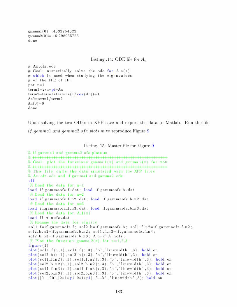
gamma1(0)=.4532754622gamma2(0)=−6.298935755done

Listing .14: ODE file for An

# An ofz . ode# Goal : numer i ca l ly s o l v e the ode f o r A n ( z )# which i s used when studying the e i g e n v a l u e s# o f the FPE of IF .par n=1term1=2∗n∗ pi+Anterm2=term1∗ term1 ∗(1/ cos (An))+ tAn’=term1/term2An(0)=0done

Upon solving the two ODEs in XPP save and export the data to Matlab. Run the file

if gamma1 and gamma2 ofz plots.m to reproduce Figure 9

Listing .15: Master file for Figure 9

% if gamma1 and gamma2 ofz plots .m% ++++++++++++++++++++++++++++++++++++++++++++++++++++++++++% Goal : p l o t the f u n c t i o n s gamma 1( z ) and gamma 2( z ) f o r z>0% ++++++++++++++++++++++++++++++++++++++++++++++++++++++++++% This f i l e c a l l s the data s imulated with the XPP f i l e s% An ofz . ode and if gamma1 and gamma2 . odec l f% Load the data f o r n=1

load i f gammaofz f . dat ; load i f gammaofz b . dat% Load the data f o r n=2

load i f gammaofz f n2 . dat ; load i f gammaofz b n2 . dat% Load the data f o r n=3

load i f gammaofz f n3 . dat ; load i f gammaofz b n3 . dat% Load the data f o r A 1 ( z )

load i f A n o f z . dat% Rename the data f o r c l a r i t y

s o l 1 f=i f gammaofz f ; s o l 2 b=if gammaofz b ; s o l 1 f n 2=i f gammaofz f n2 ;s o l 2 b n 2=if gammaofz b n2 ; s o l 1 f n 3=i f gammaofz f n3 ;s o l 2 b n 3=if gammaofz b n3 ; A n=i f A n o f z ;% Plot the func t i on gamma 2( z ) f o r n=1 ,2 ,3

f i g u r e (1 )p l o t ( s o l 1 f ( : , 1 ) , s o l 1 f ( : , 3 ) , ’ b ’ , ’ l i n ew id th ’ , 3 ) ; hold onp lo t ( s o l 2 b ( : , 1 ) , s o l 2 b ( : , 3 ) , ’ b ’ , ’ l i n ew id th ’ , 3 ) ; hold onp lo t ( s o l 1 f n 2 ( : , 1 ) , s o l 1 f n 2 ( : , 3 ) , ’ b ’ , ’ l i n ew id th ’ , 3 ) ; hold onp lo t ( s o l 2 b n 2 ( : , 1 ) , s o l 2 b n 2 ( : , 3 ) , ’ b ’ , ’ l i n ew id th ’ , 3 ) ; hold onp lo t ( s o l 1 f n 3 ( : , 1 ) , s o l 1 f n 3 ( : , 3 ) , ’ b ’ , ’ l i n ew id th ’ , 3 ) ; hold onp lo t ( s o l 2 b n 3 ( : , 1 ) , s o l 2 b n 3 ( : , 3 ) , ’ b ’ , ’ l i n ew id th ’ , 3 ) ; hold onp lo t ( [ 0 1 2 0 ] , [ 2∗1∗ pi 2∗1∗ pi ] , ’−−k ’ , ’ l i n ew id th ’ , 3 ) ; hold on

183

p lo t ( [ 0 1 2 0 ] , [ 2∗2∗ pi 2∗2∗ pi ] , ’−−k ’ , ’ l i n ew id th ’ , 3 ) ; hold onp lo t ( [ 0 1 2 0 ] , [ 2∗1∗ pi+pi /2 2∗1∗ pi+pi / 2 ] , ’−−k ’ , ’ l i n ew id th ’ , 3 ) ; hold onp lo t ( [ 0 1 2 0 ] , [ 2∗2∗ pi+pi /2 2∗2∗ pi+pi / 2 ] , ’−−k ’ , ’ l i n ew id th ’ , 3 ) ; hold onp lo t ( [ 0 1 2 0 ] , [ 2∗3∗ pi 2∗3∗ pi ] , ’−−k ’ , ’ l i n ew id th ’ , 3 ) ; hold onp lo t ( [ 0 1 2 0 ] , [ 2∗3∗ pi+pi /2 2∗3∗ pi+pi / 2 ] , ’−−k ’ , ’ l i n ew id th ’ , 3 ) ; hold ona x i s ( [ 0 20 5 7∗ pi + . 8 ] ) ; hold ons e t ( gca , ’ x t i c k ’ , [ 0 5 1 5 ] , ’ f o n t s i z e ’ , 2 5 ) ; hold ontext (−1.9 ,23 , ’ \gamma 2 ’ , ’ f o n t s i z e ’ , 3 0 ) ; hold ons e t ( gca , ’ y t i c k ’ , [ 0 2 5 ] , ’ f o n t s i z e ’ , 2 5 ) ; hold ontext ( 1 9 , 4 . 2 , ’ z ’ , ’ f o n t s i z e ’ , 3 0 ) ; hold ontext (16 . 5 , 2∗ pi +2.6 , ’ 5\ pi /2 ’ , ’ f o n t s i z e ’ , 2 5 ) ; hold ontext (16 . 5 , 4∗ pi +2.6 , ’ 9\ pi /2 ’ , ’ f o n t s i z e ’ , 2 5 ) ; hold ontext (−2.3 ,2∗ pi − .2 , ’ 2\ pi ’ , ’ f o n t s i z e ’ , 3 0 ) ; hold ontext (−2.3 ,2∗2∗ pi − .2 , ’ 4\ pi ’ , ’ f o n t s i z e ’ , 3 0 ) ; hold ontext (−2.3 ,2∗3∗ pi − .2 , ’ 6\ pi ’ , ’ f o n t s i z e ’ , 3 0 ) ; hold ontext (8 ,2∗ pi +2.6 , ’n=1 ’ , ’ f o n t s i z e ’ , 3 0 ) ; hold ontext (8 ,4∗ pi +2.6 , ’n=2 ’ , ’ f o n t s i z e ’ , 3 0 ) ; hold ontext (8 ,6∗ pi +2.6 , ’n=3 ’ , ’ f o n t s i z e ’ , 3 0 ) ; hold ons e t ( gca , ’ l i n ew id th ’ , 3 . 5 , ’ f o n t s i z e ’ , 3 0 ) ; hold o f f% Plot the func t i on gamma 2( z ) f o r n=1 and A 1 ( z )

f i g u r e (2 )p l o t ( s o l 1 f ( : , 1 ) , s o l 1 f ( : , 3 ) , ’ b ’ , ’ l i n ew id th ’ , 3 ) ; hold onp lo t ( s o l 2 b ( : , 1 ) , s o l 2 b ( : , 3 ) , ’ b ’ , ’ l i n ew id th ’ , 3 ) ; hold onp lo t ( s o l 1 f n 2 ( : , 1 ) , s o l 1 f n 2 ( : , 3 ) , ’ b ’ , ’ l i n ew id th ’ , 3 ) ; hold onp lo t ( s o l 2 b n 2 ( : , 1 ) , s o l 2 b n 2 ( : , 3 ) , ’ b ’ , ’ l i n ew id th ’ , 3 ) ; hold onp lo t ( s o l 1 f n 3 ( : , 1 ) , s o l 1 f n 3 ( : , 3 ) , ’ b ’ , ’ l i n ew id th ’ , 3 ) ; hold onp lo t ( s o l 2 b n 3 ( : , 1 ) , s o l 2 b n 3 ( : , 3 ) , ’ b ’ , ’ l i n ew id th ’ , 3 ) ; hold onp lo t ( A n ( : , 1 ) , A n ( : ,2)+2∗ pi , ’−−r ’ , ’ l i n ew id th ’ , 3 ) ; hold onp lo t ( A n ( : , 1 ) , A n ( : ,2)+2∗2∗ pi , ’−−r ’ , ’ l i n ew id th ’ , 3 ) ; hold onp lo t ( [ 0 1 2 0 ] , [ 2∗1∗ pi 2∗1∗ pi ] , ’−−k ’ , ’ l i n ew id th ’ , 3 ) ; hold onp lo t ( [ 0 1 2 0 ] , [ 2∗2∗ pi 2∗2∗ pi ] , ’−−k ’ , ’ l i n ew id th ’ , 3 ) ; hold onp lo t ( [ 0 1 2 0 ] , [ 2∗1∗ pi+pi /2 2∗1∗ pi+pi / 2 ] , ’−−k ’ , ’ l i n ew id th ’ , 3 ) ; hold onp lo t ( [ 0 1 2 0 ] , [ 2∗2∗ pi+pi /2 2∗2∗ pi+pi / 2 ] , ’−−k ’ , ’ l i n ew id th ’ , 3 ) ; hold onp lo t ( [ 0 1 2 0 ] , [ 2∗3∗ pi 2∗3∗ pi ] , ’−−k ’ , ’ l i n ew id th ’ , 3 ) ; hold onp lo t ( [ 0 1 2 0 ] , [ 2∗3∗ pi+pi /2 2∗3∗ pi+pi / 2 ] , ’−−k ’ , ’ l i n ew id th ’ , 3 ) ; hold ona x i s ( [ 0 22 5 5∗ pi ] ) ; hold ons e t ( gca , ’ x t i c k ’ , [ 0 5 1 5 ] , ’ f o n t s i z e ’ , 2 5 ) ; hold ons e t ( gca , ’ y t i c k ’ , [ 0 2 5 ] , ’ f o n t s i z e ’ , 2 5 ) ; hold ontext (−2.4 ,2∗ pi +.1 , ’ 2\ pi ’ , ’ f o n t s i z e ’ , 3 0 ) ; hold ontext (−2.4 ,2∗2∗ pi +.1 , ’ 4\ pi ’ , ’ f o n t s i z e ’ , 3 0 ) ; hold ontext (−1.8 , p i +.1 , ’ \ pi ’ , ’ f o n t s i z e ’ , 3 0 ) ; hold ontext (17 . 7 , 2∗ pi +2.3 , ’ 5\ pi /2 ’ , ’ f o n t s i z e ’ , 2 5 ) ; hold ontext (17 . 7 , 4∗ pi +2.3 , ’ 9\ pi /2 ’ , ’ f o n t s i z e ’ , 2 5 ) ; hold ontext ( −2 .3 ,15 .5 , ’ \gamma 2 ’ , ’ f o n t s i z e ’ , 3 0 ) ; hold ontext ( 2 1 , 4 . 3 5 , ’ z ’ , ’ f o n t s i z e ’ , 3 0 ) ; hold ontext ( 8 . 5 , 2∗ pi +2.3 , ’n=1 ’ , ’ f o n t s i z e ’ , 3 0 ) ; hold ontext ( 8 . 5 , 4∗ pi +2.3 , ’n=2 ’ , ’ f o n t s i z e ’ , 3 0 ) ; hold ons e t ( gca , ’ l i n ew id th ’ , 3 . 5 , ’ f o n t s i z e ’ , 3 0 ) ; hold o f f% Plot the func t i on gamma 1( z ) f o r n=1,2

f i g u r e (3 )p l o t ( s o l 2 b ( : , 1 ) , s o l 2 b ( : , 2 ) , ’ l i n ew id th ’ , 3 ) ; hold onp lo t ( s o l 1 f ( : , 1 ) , s o l 1 f ( : , 2 ) , ’ l i n ew id th ’ , 3 ) ; hold onp lo t ( s o l 1 f n 2 ( : , 1 ) , s o l 1 f n 2 ( : , 2 ) , ’−−r ’ , ’ l i n ew id th ’ , 3 ) ; hold onp lo t ( s o l 2 b n 2 ( : , 1 ) , s o l 2 b n 2 ( : , 2 ) , ’−−r ’ , ’ l i n ew id th ’ , 3 ) ; hold on

184

a x i s ( [ 0 1 0 2 ] ) ; hold ontext ( .95 , − . 1 , ’ z ’ , ’ f o n t s i z e ’ , 3 0 ) ; hold ontext ( . 2 2 , 1 , ’n=1 ’ , ’ f o n t s i z e ’ , 3 2 ) ; hold ontext ( . 6 , . 9 6 , ’n=2 ’ , ’ f o n t s i z e ’ , 3 2 ) ; hold ontext ( − . 074 ,1 .9 , ’ \gamma 1 ’ , ’ f o n t s i z e ’ , 3 0 ) ; hold ons e t ( gca , ’ x t i c k ’ , [ 0 . 25 . 7 5 ] , ’ f o n t s i z e ’ , 2 5 ) ; hold ons e t ( gca , ’ y t i c k ’ , [ 0 1 ] , ’ f o n t s i z e ’ , 2 5 ) ; hold ons e t ( gca , ’ l i n ew id th ’ , 3 . 5 , ’ f o n t s i z e ’ , 3 0 ) ; hold o f f% Plot gamma 1( z ) aga in s t gamma 2( z )

f i g u r e (4 )p l o t ( s o l 2 b ( : , 2 ) , s o l 2 b ( : , 3 ) , ’ l i n ew id th ’ , 3 ) ; hold onp lo t ( s o l 1 f ( : , 2 ) , s o l 1 f ( : , 3 ) , ’ l i n ew id th ’ , 3 ) ; hold onp lo t ( [ 0 1 2 0 ] , [ 2∗1∗ pi 2∗1∗ pi ] , ’−−k ’ , ’ l i n ew id th ’ , 3 ) ; hold ona x i s ( [ 0 25 5 .5 7 ] ) ; hold ons e t ( gca , ’ x t i c k ’ , [ 0 10 2 0 ] , ’ f o n t s i z e ’ , 2 5 ) ; hold ons e t ( gca , ’ y t i c k ’ , [ 0 1 0 ] , ’ f o n t s i z e ’ , 2 5 ) ; hold ontext ( 2 3 , 5 . 4 , ’ \gamma 1 ’ , ’ f o n t s i z e ’ , 3 0 ) ; hold ontext (−2.2 ,7 , ’ \gamma 2 ’ , ’ f o n t s i z e ’ , 3 0 ) ; hold ontext (−2.3 ,2∗ pi , ’ 2\ pi ’ , ’ f o n t s i z e ’ , 2 5 ) ; hold ontext (17 . 5 , 2∗ pi +1.1 , ’ A 1 ( z ) ’ , ’ f o n t s i z e ’ , 2 5 ) ; hold ontext (10 ,2∗ pi +1.8 , ’n=1 ’ , ’ f o n t s i z e ’ , 3 5 ) ; hold ons e t ( gca , ’ l i n ew id th ’ , 3 . 5 , ’ f o n t s i z e ’ , 3 0 ) ; hold onp lo t ( [ 3 3 ] , [ 2 ∗ pi +.25 2∗ pi +.25 ] , ’ og ’ , ’ l i n ew id th ’ , 9 ) ; hold ons e t ( gca , ’ l i n ew id th ’ , 3 . 5 , ’ f o n t s i z e ’ , 3 0 ) ; hold o f f% Save the p l o t s

% pr in t −f 1 −depsc2 g 2 o f z . eps% pr in t −f 2 −depsc2 g2 ofz andA n . eps% pr in t −f 3 −depsc2 g 1 o f z . eps% pr in t −f 4 −depsc2 g 1 v g 2 o f z . eps

How to reproduce Figure 10

Run the ode file if g1 g2 zpos.ode (see Listing .13) in XPP and export the saved data to

the Matlab file if lambda1 and lambda2 ofz plots.m found below in Listing .16.

Listing .16: Master file for Figure 10

% i f l ambda1 and lambda2 o f z p l o t s .m% Goal : Use the gamma data s imulated% with the xpp f i l e i f g 1 g 2 z p o s . ode% to p lo t the f u n c t i o n s lambda 1 ( z )% and lambda 2 ( z )% Clear any cur rent f i g u r e sc l f

% Load the data f o r n=1load i f gammaofz f . dat ; load i f gammaofz b . dat% Load the data f o r n=2load i f gammaofz f n2 . dat ; load i f gammaofz b n2 . dat% Load the data f o r n=3load i f gammaofz f n3 . dat ; load i f gammaofz b n3 . dat

185

% Load the data f o r A 1 ( z )load i f A n o f z . dat% Rename the data f o r c l a r i t ygamma f n1=i f gammaofz f ; gamma b n1=if gammaofz b ;gamma f n2=i f gammaofz f n2 ; gamma b n2=if gammaofz b n2 ;gamma f n3=i f gammaofz f n3 ; gamma b n3=if gammaofz b n3 ;A n=i f A n o f z ;% Def ine the parameterstheta =1; sigma =1; mu=1; z=mu∗ theta /( sigma ˆ 2 ) ;% Def ine the func t i on lambda ( z )term1=sigma ˆ4∗( gamma f n1 ( : , 2 ) . ˆ2 − gamma f n1 ( : , 3 ) . ˆ 2 ) − . . .

sigma ˆ4 .∗ gamma f n1 ( : , 1 ) . ˆ 2 ;l ambda f n1 r=term1 /(2∗ theta ˆ2∗ sigma ˆ 2 ) ;

term2=sigma ˆ4∗( gamma b n1 ( : , 2 ) . ˆ2 − gamma b n1 ( : , 3 ) . ˆ 2 ) − . . .sigma ˆ4 .∗ gamma b n1 ( : , 1 ) . ˆ 2 ;

lambda b n1 r=term2 /(2∗ theta ˆ2∗ sigma ˆ 2 ) ;

term3=sigma ˆ4∗( gamma f n2 ( : , 2 ) . ˆ2 − gamma f n2 ( : , 3 ) . ˆ 2 ) − . . .sigma ˆ4 .∗ gamma f n2 ( : , 1 ) . ˆ 2 ;

l ambda f n2 r=term3 /(2∗ theta ˆ2∗ sigma ˆ 2 ) ;

term4=sigma ˆ4∗( gamma b n2 ( : , 2 ) . ˆ2 − gamma b n2 ( : , 3 ) . ˆ 2 ) − . . .sigma ˆ4 .∗ gamma b n2 ( : , 1 ) . ˆ 2 ;

lambda b n2 r=term4 /(2∗ theta ˆ2∗ sigma ˆ 2 ) ;

term5=sigma ˆ4∗( gamma f n3 ( : , 2 ) . ˆ2 − gamma f n3 ( : , 3 ) . ˆ 2 ) − . . .sigma ˆ4 .∗ gamma f n3 ( : , 1 ) . ˆ 2 ;

l ambda f n3 r=term5 /(2∗ theta ˆ2∗ sigma ˆ 2 ) ;

term6=sigma ˆ4∗( gamma b n3 ( : , 2 ) . ˆ2 − gamma b n3 ( : , 3 ) . ˆ 2 ) − . . .sigma ˆ4 .∗ gamma b n3 ( : , 1 ) . ˆ 2 ;

lambda b n3 r=term6 /(2∗ theta ˆ2∗ sigma ˆ 2 ) ;% Plot the f u n c t i o n s Re ( lambda ( z ) )f i g u r e (1 )p l o t ( gamma f n1 ( : , 1 ) , lambda f n1 r , ’b ’ , ’ l i n ew id th ’ , 4 ) ; hold onp lo t ( gamma b n1 ( : , 1 ) , lambda b n1 r , ’b ’ , ’ l i n ew id th ’ , 4 ) ; hold onp lo t ( gamma f n2 ( : , 1 ) , lambda f n2 r , ’ k ’ , ’ l i n ew id th ’ , 4 ) ; hold onp lo t ( gamma b n2 ( : , 1 ) , lambda b n2 r , ’ k ’ , ’ l i n ew id th ’ , 4 ) ; hold onp lo t ( gamma f n3 ( : , 1 ) , lambda f n3 r , ’ g ’ , ’ l i n ew id th ’ , 4 ) ; hold onp lo t ( gamma b n3 ( : , 1 ) , lambda b n3 r , ’ g ’ , ’ l i n ew id th ’ , 4 ) ; hold onp lo t ([−5 5] , [−2∗1∗ pi ˆ2 −2∗1∗pi ˆ 2 ] , ’−−k ’ , ’ l i n ew id th ’ , 3 ) ; hold onp lo t ([−5 5] , [−2∗2ˆ2∗ pi ˆ2 −2∗2ˆ2∗ pi ˆ 2 ] , ’−−k ’ , ’ l i n ew id th ’ , 3 ) ; hold onp lo t ([−5 5] , [−2∗3ˆ2∗ pi ˆ2 −2∗3ˆ2∗ pi ˆ 2 ] , ’−−k ’ , ’ l i n ew id th ’ , 3 ) ; hold ons e t ( gca , ’ x t i c k ’ , [ 0 2 4 ] , ’ f o n t s i z e ’ , 2 0 ) ; hold ons e t ( gca , ’ y t i c k ’ ,[−200 −150 −100 −50 0 ] , ’ f o n t s i z e ’ , 2 0 ) ; hold ontext (4.7 ,−263 , ’ z ’ , ’ f o n t s i z e ’ , 3 0 ) ; hold ontext (− .47 ,41 , ’ \ lambda 1 ’ , ’ f o n t s i z e ’ , 3 0 ) ; hold ons e t ( gca , ’ l i n ew id th ’ , 3 . 5 , ’ f o n t s i z e ’ , 3 0 ) ; hold ona x i s ( [ 0 5 −250 5 0 ] ) ; hold o f f% Def ine the func t i on IM lambda ( z )lambda f n1 im=gamma f n1 ( : , 2 ) . ∗ gamma f n1 ( : , 3 ) ;lambda b n1 im=gamma b n1 ( : , 2 ) . ∗ gamma b n1 ( : , 3 ) ;lambda f n2 im=gamma f n2 ( : , 2 ) . ∗ gamma f n2 ( : , 3 ) ;

186

lambda b n2 im=gamma b n2 ( : , 2 ) . ∗ gamma b n2 ( : , 3 ) ;lambda f n3 im=gamma f n3 ( : , 2 ) . ∗ gamma f n3 ( : , 3 ) ;lambda b n3 im=gamma b n3 ( : , 2 ) . ∗ gamma b n3 ( : , 3 ) ;% p lo t the In ( lambda ( z ) )f i g u r e (2 )p l o t ( gamma f n1 ( : , 1 ) , lambda f n1 im , ’b ’ , ’ l i n ew id th ’ , 3 ) ; hold onp lo t ( gamma b n1 ( : , 1 ) , lambda b n1 im , ’b ’ , ’ l i n ew id th ’ , 3 ) ;p l o t ( gamma f n2 ( : , 1 ) , lambda f n2 im , ’ k ’ , ’ l i n ew id th ’ , 3 ) ;p l o t ( gamma b n2 ( : , 1 ) , lambda b n2 im , ’ k ’ , ’ l i n ew id th ’ , 3 ) ;p l o t ( gamma f n3 ( : , 1 ) , lambda f n3 im , ’ g ’ , ’ l i n ew id th ’ , 3 ) ;p l o t ( gamma b n3 ( : , 1 ) , lambda b n3 im , ’ g ’ , ’ l i n ew id th ’ , 3 ) ;p l o t ( gamma f n1 ( : ,1) , − lambda f n1 im , ’b ’ , ’ l i n ew id th ’ , 3 ) ;p l o t ( gamma b n1 ( : ,1) , − lambda b n1 im , ’b ’ , ’ l i n ew id th ’ , 3 ) ;p l o t ( gamma f n2 ( : ,1) , − lambda f n2 im , ’ k ’ , ’ l i n ew id th ’ , 3 ) ;p l o t ( gamma b n2 ( : ,1) , − lambda b n2 im , ’ k ’ , ’ l i n ew id th ’ , 3 ) ;p l o t ( gamma f n3 ( : ,1) , − lambda f n3 im , ’ g ’ , ’ l i n ew id th ’ , 3 ) ;p l o t ( gamma b n3 ( : ,1) , − lambda b n3 im , ’ g ’ , ’ l i n ew id th ’ , 3 ) ;p l o t ([−5 0 ] , [ 0 0 ] , ’ k ’ , ’ l i n ew id th ’ , 4 ) ;t ex t (3.7 ,−132 , ’ z ’ , ’ f o n t s i z e ’ , 3 0 ) ;%text (−6 ,110 , ’\ lambda 2 ’ , ’ f o n t s i z e ’ , 3 0 ) ;s e t ( gca , ’ x t i c k ’ ,[−5 0 5 ] , ’ f o n t s i z e ’ , 2 0 ) ;s e t ( gca , ’ y t i c k ’ ,[−100 −50 0 50 100 ] , ’ f o n t s i z e ’ , 1 5 ) ;s e t ( gca , ’ l i n ew id th ’ , 3 . 5 , ’ f o n t s i z e ’ , 3 0 ) ;t i t l e ( ’ Im(\ lambda ( z ) ) ’ ) ;a x i s ([−5 5 −120 1 2 0 ] ) ; hold o f f%% Load the XPP dataload IF muneg gamma1 . dat ; load IF muneg gamma1 . datload IF muneg gamma2 . dat ; load IF muneg gamma2 . datload IF muneg gamma3 . dat ; load IF muneg gamma3 . datload IF muneg gamma4 . dat ; load IF muneg gamma4 . dat% Rename the data f o r conveniencep=IF muneg gamma1 ; n=IF muneg gamma1 ;q=IF muneg gamma2 ; r=IF muneg gamma2 ;s=IF muneg gamma3 ; t=IF muneg gamma3 ;u=IF muneg gamma4 ; v=IF muneg gamma4 ;% Check the s i z e o f the matrix p .s i z e (p ) ;

% Def ine the f u n c t i o n s lambda ( z )y1=−(p ( : , 2 ) . ∗ p ( : ,2 )+ p ( : , 1 ) . ∗ p ( : , 1 ) ) . / 2 ;y2=−(n ( : , 2 ) . ∗ n ( : ,2 )+ n ( : , 1 ) . ∗ n ( : , 1 ) ) . / 2 ;y3=−(q ( : , 2 ) . ∗ q ( : ,2 )+ q ( : , 1 ) . ∗ q ( : , 1 ) ) . / 2 ;y4=−(r ( : , 2 ) . ∗ r ( : , 2 )+ r ( : , 1 ) . ∗ r ( : , 1 ) ) . / 2 ;y5=−(s ( : , 2 ) . ∗ s ( : , 2 )+ s ( : , 1 ) . ∗ s ( : , 1 ) ) . / 2 ;y6=−(t ( : , 2 ) . ∗ t ( : , 2 )+ t ( : , 1 ) . ∗ t ( : , 1 ) ) . / 2 ;y7=−(u ( : , 2 ) . ∗ u ( : ,2 )+ u ( : , 1 ) . ∗ u ( : , 1 ) ) . / 2 ;y8=−(v ( : , 2 ) . ∗ v ( : ,2 )+ v ( : , 1 ) . ∗ v ( : , 1 ) ) . / 2 ;f i g u r e (3 )p l o t ( gamma f n1 ( : , 1 ) , lambda f n1 r , ’b ’ , ’ l i n ew id th ’ , 4 ) ; hold onp lo t ( gamma b n1 ( : , 1 ) , lambda b n1 r , ’b ’ , ’ l i n ew id th ’ , 4 ) ;p l o t ( gamma f n2 ( : , 1 ) , lambda f n2 r , ’ k ’ , ’ l i n ew id th ’ , 4 ) ;p l o t ( gamma b n2 ( : , 1 ) , lambda b n2 r , ’ k ’ , ’ l i n ew id th ’ , 4 ) ;p l o t ( gamma f n3 ( : , 1 ) , lambda f n3 r , ’ g ’ , ’ l i n ew id th ’ , 4 ) ;p l o t ( gamma b n3 ( : , 1 ) , lambda b n3 r , ’ g ’ , ’ l i n ew id th ’ , 4 ) ;

187

p lo t (p ( : , 1 ) , y1 , ’b ’ , ’ l i n ew id th ’ , 3 . 5 ) ;p l o t (n ( : , 1 ) , y2 , ’b ’ , ’ l i n ew id th ’ , 3 . 5 ) ;p l o t ( q ( : , 1 ) , y3 , ’b ’ , ’ l i n ew id th ’ , 3 . 5 ) ;p l o t ( r ( : , 1 ) , y4 , ’b ’ , ’ l i n ew id th ’ , 3 . 5 ) ;p l o t ( s ( : , 1 ) , y5 , ’ k ’ , ’ l i n ew id th ’ , 3 . 5 ) ;p l o t ( t ( : , 1 ) , y6 , ’ k ’ , ’ l i n ew id th ’ , 3 . 5 ) ;p l o t (u ( : , 1 ) , y7 , ’ k ’ , ’ l i n ew id th ’ , 3 . 5 ) ;p l o t ( v ( : , 1 ) , y8 , ’ k ’ , ’ l i n ew id th ’ , 3 . 5 ) ;p l o t ([−5 5] , [−2∗1∗ pi ˆ2 −2∗1∗pi ˆ 2 ] , ’−−r ’ , ’ l i n ew id th ’ , 2 . 5 ) ;p l o t ([−5 5] , [−2∗2ˆ2∗ pi ˆ2 −2∗2ˆ2∗ pi ˆ 2 ] , ’−−r ’ , ’ l i n ew id th ’ , 2 . 5 ) ;p l o t ([−5 5] , [−2∗3ˆ2∗ pi ˆ2 −2∗3ˆ2∗ pi ˆ 2 ] , ’−−r ’ , ’ l i n ew id th ’ , 3 ) ;s e t ( gca , ’ x t i c k ’ ,[−5 0 5 ] , ’ f o n t s i z e ’ , 2 0 ) ;s e t ( gca , ’ y t i c k ’ ,[−100 −50 0 ] , ’ f o n t s i z e ’ , 2 0 ) ;t ex t (3.7 ,−122 , ’ z ’ , ’ f o n t s i z e ’ , 3 0 ) ;%text (−5.47 ,0 , ’\ lambda 1 ’ , ’ f o n t s i z e ’ , 3 0 ) ;s e t ( gca , ’ l i n ew id th ’ , 3 . 5 , ’ f o n t s i z e ’ , 3 0 ) ;t i t l e ( ’Re(\ lambda ( z ) ) ’ ) ;a x i s ([−5 5 −115 0 ] ) ; hold o f f

%pr in t −f 1 −depsc2 l ambda rea l z pos . eps%pr in t −f 2 −depsc2 lambda im z pos . epsp r i n t −f 2 −depsc2 d e f 1 . epsp r i n t −f 3 −depsc2 d e f 2 . eps

A.4 CALCULATING THE EIGENVALUES FOR THE FPE OF THE IF

MODEL

First, define the function file nonlinear FandG if.m which defines the nonlinear algebra

problem (F,G) = (0, 0). Next, run the Matlab file gamma and evalues IF.m to calculate

the γ and λ values listed in Tables 1-8.

Listing .17: M-file for calculating the Eigenvalues

% gamma and evalues IF .m% Goal : Ca l cu la t e the gamma va lue s ( and hence eva lue s ) o f the IF when% V L=V R=0 and V T=theta .%+++++++++++++++++++++++++++++++++++++++++++++++++++++++++++++++t i c % Set the t imermu=0.001; theta =1; sigma =5; % Set parametersz1=mu∗ theta /( sigma∗ sigma ) ; % Set z f o r gammaˆ s t a rg s t a r=log ( exp ( z1)+ s q r t ( exp (2∗ z1 )−1)) ; %+++++++++++++++++++++gamma1old=gs ta r ; % Set I n i t i a l gue s s e s%gamma1old=0 % i f mu<0gamma2old =6.4 ; %+++++++++++++++++++++%gamma2old=3.3 % i f mu<0

188

numberofe igenvalues =10; % How many e i g e n v a l u e s do we want% Set the s o l u t i o n matr i ce s .o ld=ze ro s ( numberofe igenvalues , 5 ) ;gammavalues=ze ro s ( numberofe igenvalues , 4 ) ;newsol=ze ro s ( 1 , 2 ) ;% Set i n i t i a l i z e Guesseso ld (1 ,2)=gamma1old ; o ld (1 ,3)=gamma2old ;gamma1old=old ( 1 , 2 ) ; gamma2old (1 ,3)= old ( 1 , 3 ) ;f o r i =1: numberofe igenvaluesmyf 1=@(gamma) nonl inear FandG IF (gamma,mu, theta , sigma ) ;opt ions=opt imset ( ’ Display ’ , ’ o f f ’ ) ;s o l=f s o l v e ( myf 1 , [ gamma1old gamma2old ] , opt i ons ) ;% Check we a c t u a l l y found a s o l u t i o nCheck=nonlinear FandG IF ( [ s o l (1 ) s o l ( 2 ) ] ,mu, theta , sigma ) ;gammavalues ( i ,1)= s o l ( 1 ) ;gammavalues ( i ,2)= s o l ( 2 ) ;gammavalues ( i ,3)= Check ( 1 ) ;gammavalues ( i ,4)= Check ( 2 ) ;gamma1old=s o l ( 1 ) ;% gamma2old=s o l (2 )+6 .4 ;gamma2old=s o l (2)+ pi ; % i f mu<0% Save the gamma va lue s in the matrix o ldo ld ( i ,1)=mu;o ld ( i ,2)= s o l ( 1 ) ;o ld ( i ,3)= s o l ( 2 ) ;%check e r r o ro ld ( i ,4)= Check ( 1 ) ;o ld ( i ,5)= Check ( 2 ) ;endold ; gammavalues ;% Def ine the gamma va lue sgammadata=[gammavalues ( : , 1 ) gammavalues ( : , 2 ) ]% Save the gamma va lue s

save gammavalues mupt001 sigma5 . dat −a s c i i gammadata% Calcu la te the r e a l par t s o f the e i g e n v a l u e sterm1=sigma ˆ ( 4 ) . ∗ ( o ld ( : , 2 ) . ∗ o ld ( : ,2)− o ld ( : , 3 ) . ∗ o ld ( : , 3 ) ) . . .

−mu∗mu∗ theta ∗ theta ;term2=2∗ theta ∗ theta ∗ sigma∗ sigma ;lambdareal=term1 . / term2 ;% Calcu la te the imaginary par t sterm3=old ( : , 2 ) . ∗ o ld ( : , 3 ) . ∗ sigma∗ sigma ;lambdaim=term3 /( theta ∗ theta ) ;% Def ine the matrix o f e i g e n v a l u e se i g e n v a l u e s =[ lambdareal lambdaim ]% Save the e i g e n v a l u e s

save evalues mupt001 s igma5 . dat −a s c i i e i g e n v a l u e stoc

189

A.5 THE FIRING RATE FUNCTION

In this section we provide Matlab code to plot the theoretical firing rate and the population

firing rate.

A.5.1 Calculating the Theoretical Firing Rate, ν(t)

To reproduce Figure 12 five programs are needed. First we need three function files (see

Listings .18-.19-.20).

Listing .18: Function file for the Eigenfunction φ′n(V )

% phipr ime gene ra l .m

% This func t i on f i l e i s used in the f i l e t h e o r y f i r i n g r a t e I F .m% to determine the value o f the d e r i v a t i v e o f the% e i g e n f u n c t i o n phi n .f unc t i on y=ph ipr ime gene ra l (v , gammaval ,mu, sigma , theta )% Def ine zz=mu.∗ theta . / ( sigma .∗ sigma ) ;% Begin d e f i n i n g phi nterm1=exp ( z .∗ v . / theta ) ;term2=(z . / theta ) . ∗ s inh ( gammaval . ∗ ( theta−v ) . / theta ) ;term3=(gammaval . / theta ) . ∗ cosh ( gammaval . ∗ ( theta−v ) . / theta ) ;% Def ine the constant c lambdaterm4=gammaval .∗ z .∗ cosh ( gammaval ) ;term5=(gammaval .∗ gammaval−z ) . ∗ s inh ( gammaval ) ;term6=theta . ∗ ( term4+term5 ) ;csublambda =2.∗gammaval . / term6 ;y=(csublambda ) . ∗ term1 . ∗ ( term2−term3 ) ;

Listing .19: Function file for the Eigenfunction φ′0(V )

% ph i z e rop r ime gene ra l .m

% This func t i on f i l e i s used in the f i l e t h e o r y f i r i n g r a t e I F .m% to determine the value o f the d e r i v a t i v e o f the% e i g e n f u n c t i o n p h i z e r o .f unc t i on y=ph i z e rop r ime gene ra l (v ,mu, sigma , theta )% Def ine zz=mu.∗ theta . / ( sigma .∗ sigma ) ;% Def ine the constantc o e f =(sigma .∗ sigma ) . / ( 2 . ∗mu.∗mu) ;c1=c o e f . ∗ ( 2 . ∗mu.∗ theta . / ( sigma .∗ sigma ) − 1 . . . .

+exp (−2.∗mu.∗ theta . / ( sigma .∗ sigma ) ) ) ;cAA=1./ c1 ;

190

term1000= −2.∗(cAA. / ( sigma .∗ sigma ) ) . ∗ exp (−2.∗ z . ∗ ( theta−v ) . / theta ) ;y=term1000 ;

Listing .20: Function file for the Eigenfunction ψ(V )

% p s i g e n e r a l .m

% This func t i on f i l e i s used in the f i l e t h e o r y f i r i n g r a t e I F .m% to determine the value o f the o f the func t i on p s i n .f unc t i on y=p s i g e n e r a l (v , gammaval ,mu, sigma , theta )% Def ine zz=mu.∗ theta . / ( sigma .∗ sigma ) ;term1=exp(−z .∗ v . / theta ) ;termA=sinh ( gammaval .∗ v . / theta ) ;termB=cosh ( gammaval .∗ v . / theta ) ;y=term1 . ∗ ( gammaval .∗ termB+z .∗ termA ) ;

Next, export the eigenvalue data saved in Listing .17 to the following code:

Listing .21: Driver for Figure 12

% t h e o r y f i r i n g r a t e I F .m% Goal : Ca l cu la t e the t h e o r e t i c a l f i r i n g ra t e nu( t ) o f the IF neuron% when V L=V R=0. This program c a l l s data from gamma and evalues IF .m% I t uses the func t i on f i l e s ph i z e rop r ime gene ra l .m,% ph ipr ime gene ra l .m and p s i g e n e r a l .m%++++++++++++++++++++++++++++++++++++++++++++++++++++++++c l f % Clear a l l f i g u r e s and va luest i c % Set the t imer

%======== Load the gamma and lambda va lue s===============load gammavalues mupt05 sigma5 . datload evalues mupt05 s igma5 . datgammaval11=gammavalues mupt05 sigma5 ;lambdavalues11=evalues mupt05 s igma5 ;% Def ine the v e c t o r s o f r e a l par t s o f gamma/lamba

realgamma=gammaval11 ( : , 1 ) ; real lambda=lambdavalues11 ( : , 1 ) ;% Def ine the v e c t o r s o f imaginary par t s o f gamma/lambda

imaggamma=gammaval11 ( : , 2 ) ; imaglambda=lambdavalues11 ( : , 2 ) ;% Def ine the vec to r o f complex gamma va lue s .

gammavals=gammaval11 ( : ,1 )+1 i ∗gammaval11 ( : , 2 ) ;gammavals conj=gammaval11 ( : ,1)−1 i ∗gammaval11 ( : , 2 ) ;

% Def ine the vec to r o f complex lambda va lue s .lambdavals=lambdavalues11 ( : ,1 )+1 i ∗ lambdavalues11 ( : , 2 ) ;lambdaval s conj=lambdavalues11 ( : ,1)−1 i ∗ lambdavalues11 ( : , 2 ) ;

%=========================================================t =0 : . 0001 : 100 ; % Set the domain o f nu( t ) .mu=.05; % Set the c o r r e c t mu, theta and sigma va lue s .sigma =5; theta =1; v0=0;%−−−−−−−−−−−−−−−−−−−−Def ine nu( t)−−−−−−−−−−−−−−−−−−−−−−−−% Set the f i r s t term in the f i r i n g ra t e : −sigma ˆ2/2

191

term1=−(sigma∗ sigma ) / 2 ;% The f i r s t term in the expansionterm2=ph i z e rop r ime gene ra l ( theta ,mu, sigma , theta ) ;% Check that our l i m i t i n g value i s c o r r e c tp r e d i c t i o n=term1∗ term2B=p r e d i c t i o n ;% The f i r s t term in the expansion ( and conj )term3=exp ( lambdaval s conj (1)∗ t ) ∗ . . .

ph ip r ime gene ra l ( theta , gammavals conj ( 1 ) ,mu, sigma , theta ) ;term4=exp ( lambdavals (1)∗ t ) ∗ . . .

ph ip r ime gene ra l ( theta , gammavals ( 1 ) ,mu, sigma , theta ) ;term5=p s i g e n e r a l ( v0 , gammavals ( 1 ) ,mu, sigma , theta ) ;term6=p s i g e n e r a l ( v0 , gammavals conj ( 1 ) ,mu, sigma , theta ) ;

% The second term in the expansion ( and conj )term31=exp ( lambdava l s conj (2)∗ t ) ∗ . . .

ph ip r ime gene ra l ( theta , gammavals conj ( 2 ) ,mu, sigma , theta ) ;term41=exp ( lambdavals (2)∗ t ) ∗ . . .

ph ip r ime gene ra l ( theta , gammavals ( 2 ) ,mu, sigma , theta ) ;term51=p s i g e n e r a l ( v0 , gammavals ( 2 ) ,mu, sigma , theta ) ;term61=p s i g e n e r a l ( v0 , gammavals conj ( 2 ) ,mu, sigma , theta ) ;

% The th i rd term in the expansion ( and conj )term32=exp ( lambdava l s conj (3)∗ t ) ∗ . . .

ph ip r ime gene ra l ( theta , gammavals conj ( 3 ) ,mu, sigma , theta ) ;term42=exp ( lambdavals (3)∗ t ) ∗ . . .

ph ip r ime gene ra l ( theta , gammavals ( 3 ) ,mu, sigma , theta ) ;term52=p s i g e n e r a l ( v0 , gammavals ( 3 ) ,mu, sigma , theta ) ;term62=p s i g e n e r a l ( v0 , gammavals conj ( 3 ) ,mu, sigma , theta ) ;

% The four th term in the expansion ( and conj )term33=exp ( lambdava l s conj (4)∗ t ) ∗ . . .

ph ip r ime gene ra l ( theta , gammavals conj ( 4 ) ,mu, sigma , theta ) ;term43=exp ( lambdavals (4)∗ t ) ∗ . . .

ph ip r ime gene ra l (1 , gammavals ( 4 ) ,mu, sigma , theta ) ;term53=p s i g e n e r a l ( v0 , gammavals ( 4 ) ,mu, sigma , theta ) ;term63=p s i g e n e r a l ( v0 , gammavals conj ( 4 ) ,mu, sigma , theta ) ;

% Def ine the f i r i n g ra t e nu( t )nu=term1 ∗( term2+term3∗ term6+term4∗ term5 + . . .

term31∗ term61+term41∗ term51 + . . .term32∗ term62+term42∗ term52 + . . .

term33∗ term63+term43∗ term53 ) ;% This expansion i s f o r the f i r s t f our e i g e n v a l u e s .% This works but i t i s too long to put in .% Need a more e f f e c i e n t way to ente r the f u n c t i o n s .

% Save the func t i on nu( t ) f o r each mu.So l data =[1000∗ t ; nu ] ;%save t h e o r y f i r i n g r a t e m u 2 0 . dat −a s c i i So l data%save t h e o r y f i r i n g r a t e m u 5 . dat −a s c i i So l data%save t h e o r y f i r i n g r a t e m u 1 . dat −a s c i i So l data%save t h e o r y f i r i n g r a t e m u p t 1 . dat −a s c i i So l data%save t h e o r y f i r i n g r a t e m u 2 5 s i g m a 1 0 . dat −a s c i i So l data

192

%save t h e o r y f i r i n g r a t e m u p t 1 s i g m a 5 . dat −a s c i i So l data

%++++++++++++++Plot the f i r i n g ra t e++++++++++++++++++++++++++f i g u r e (1 )p l o t ( So l data ( 1 , : ) , So l data ( 2 , : ) , ’ l i n ew id th ’ , 4 . 5 ) ; hold onp lo t ( So l data ( 1 , : ) , 0 ∗ So l data (1 , : )+B, ’−−k ’ , ’ l i n ew id th ’ , 3 . 5 ) ;s e t ( gca , ’ y t i c k ’ , [ 0 20 40 6 0 ] , ’ f o n t s i z e ’ , 25)s e t ( gca , ’ x t i c k ’ , [ 0 100 200 300 ] , ’ f o n t s i z e ’ , 25)t ex t (−25 ,58 , ’ \nu ’ , ’ f o n t s i z e ’ , 3 0 ) ;t ex t (150 ,50 , ’ \mu =0.1 , \ theta =1, \ sigma=5 ’ , ’ f o n t s i z e ’ , 2 5 ) ;t ex t (380 ,−7 , ’ t ’ , ’ f o n t s i z e ’ , 3 0 ) ;t ex t ( 1 5 0 , 4 0 , [ ’ \nu(\ i n f t y )= ’ num2str (B) ] , ’ f o n t s i z e ’ , 2 5 ) ;s e t ( gca , ’ l i n ew id th ’ , 3 . 5 , ’ f o n t s i z e ’ , 3 0 ) ;a x i s ( [ 0 400 −2 6 0 ] ) ;hold o f f%pr in t −f 1 −depsc2 theory fr mup1 . epstoc

A.5.2 Simulation of the Population Firing Rate

To simulate a population of N IF neurons and calculate the population run the Matlab file

pop firingrate IF.m below.

Caution: The simulation of 10000 neurons requires roughly 50 minutes.

Listing .22: Driver to Compute the Population Firing Rate

% p o p f i r i n g r a t e i f .m% Goal : To c a l c u l a t e the populat ion f i r i n g ra t e f o r N IF% neurons . In p a r t i c u l a r , we use t h i s f i l e to p l o t the% populat ion f i r i n g ra t e and the t h e o r e t i c a l f i r i n g ra t e% on the same a x i s . This i s s i m i l a r to Figure 2 o f Mattiac l f % Clear a l l f i g u r e s

% Set the t imer ( f o r a populat ion o f 10000 neurons% i t takes roug ly 60 minutes to compute )t i cneurons =10; % Set the number o f neuronsd e l t a= 0 . 0 0 1 ; % Set the value d e l t a th=d e l t a /100 ; % Set the s tep s i z eV T=1; % Set the th r e sho ld value V T=theta where a sp ike occursV 0=0; % Set the i n i t i a l cond i t i on V 0=V(0)V L=0; % Set the r e f l e c t i v e boundary V LV R=0; % Set the r e s e t va lue V Rmu=−1; % Set the parameters mu and sigmasigma =5; % I n i t i a l i z e the number o f s p i k e s f o r the populat ionnumberofspikes =0; % I n i t i a l i z e the number o f s p i k e s per neuroncount =0; % I n i t i a l i z e the i n i t a l TOTAL sp ike counts e c s =.5 ; % How many seconds to s imulateI I=s e c s /h ; % Set the number o f i t e r a t i o n s f o r the Euler method .

193

t imes=l i n s p a c e (0 , secs , s e c s /h+1); % Set the vec to r o f t imes f o r which% the SDE i s so lved .

V=ze ro s (1 , s e c s /h ) ; % Set the s o l u t i o n vec to r V( t ) .sp ike t imes = [ ] ; % Set the vec to r whose e n t r i e s are the sp ike t imes .

% Find the equ i l i b r i um valueterm1=−(sigma∗ sigma ) / 2 ;% The f i r s t term in the expansionterm2=ph i z e rop r ime gene ra l (V T ,mu, sigma , V T ) ;% Check that our l i m i t i n g value i s c o r r e c tn u i n f i n i t y=term1∗ term2

% Use Forward Euler to s imulate a populat ion o f neuronsf o r i =1: neurons

f o r k=1: I IV( k+1)=V( k)+h∗mu+sigma∗ s q r t (h)∗ randn ;

i f (V( k+1)<V L)V( k+1)=V R ;

end ;i f (V( k+1)>V T)

V( k)=V T ;V( k+1)=V R ;sp ike t imes =[ sp ike t imes t imes ( k ) ] ;count=count +1;numberofspikes=numberofspikes +1;

end ;end ;end ;sp ike t imes=sp ike t imes ;numberofspikes=count % Print the number o f s p i k e s f o r the populat ion .% We need to f i n d the number o f s p i k e s in each% s u b i n t e r v a l ( t , t+h ) . Reca l l that% n( t , t+h)=number o f s p i k e s in ( t , t+h ) .sub in t s=s e c s / de l t a ; % Set the number o f s u b i n t e r v a l s .va lue s=ze ro s (1 , sub in t s ) ; % Set the vec to r that shows the number o f

% s p i k e s in each o f the s u b i n t e r v a l s .% Count the number o f s p i k e s in each s u b i n t e r v a l .

f o r m=1: sub in t sf o r n=1: numberofspikes

count 1 =0;i f ( (m−1)∗ d e l t a < sp ike t imes (n ) ) ;

count 1=count 1 +1;end ;i f ( sp ike t imes (n)>m∗ d e l t a )

count 1=count 1 −1;end ;

va lue s (m)= va lue s (m)+count 1 ;end

endva lue s ;% Check that the number o f s p i k e s in each sub−% i n t e r v a l add up to the t o t a l number o f s p i k e s .t h i s b e t t e r b e z e r o=sum( va lues )−numberofspikes % you should get 0

% Def ine the populat ion f i r i n g ra t e func t i on .num f i r i ng ra t e=va lues /( neurons ∗ d e l t a ) ;

194

% Def ine the vec to r o f t imes to p l o t aga in s t the% populat ion f i r i n g ra t e func t i on .t imes 1=l i n s p a c e (0 , secs , s e c s / d e l t a ) ;% Mult ip ly the domain by 1000 to get msSo l data =[1000∗ t imes 1 ; num f i r i ng ra t e ] ;% +++++++++++++++++++++++++++++++++++++++% Save the data to p l o t with t h e o r e t i c a l .% +++++++++++++++++++++++++++++++++++++++% Make sure the c o r r e c t mu i s used ! ! ! ! ! !% +++++++++++++++++++++++++++++++++++++++% save p o p f i r i n g r a t e m u 2 0 . dat −a s c i i So l data% save p o p f i r i n g r a t e m u 5 . dat −a s c i i So l data% save p o p f i r i n g r a t e m u 1 . dat −a s c i i So l data% save p o p f i r i n g r a t e m u p t 1 . dat −a s c i i So l data% save po p f i r i n g r a t e m u 2 5 s i gm a 1 0 . dat −a s c i i So l data% save p o p f i r i n g r a t e m u p t 1 s i g m a 5 . dat −a s c i i So l data% save pop f i r i ng ra t e mu neg1 s i gma 1 . dat −a s c i i So l data% save pop f i r i ng ra t e mu neg1 s i gma 5 . dat −a s c i i So l data% +++++++++++++++++++++++++++++++++++++++% Plot the populat ion f i r i n g ra t e .% +++++++++++++++++++++++++++++++++++++++f i g u r e (1 )% Mult ip ly the domain by 1000 to use msp lo t (1000∗ t imes 1 , num f i r i ng ra t e )%a x i s ( [ 0 s e c s ∗1000 −2 6 0 ] )

load pop f i r i ng ra t e mu neg1 s i gma 5 . datp f r=pop f i r i ng ra t e mu neg1 s i gma 5 ;

f i g u r e (2 )p l o t ( p f r ( 1 , : ) , p f r ( 2 , : ) , ’ l i n ew id th ’ , 3 . 5 ) ; hold on

a x i s ( [ 0 40 −2 3 5 ] ) ; hold o f ftoc

How to Reproduce Figure 13: First, use Listing .17 to calculate the eigenvalues and store

the data. Then run the Matlab file IF firingrate pop theory.m below.

Listing .23: Driver to Plot Population and Theoretical Firing Rate

% I F f i r i n g r a t e p o p t h e o r y .mt i c ; c l f

% Load populat ion and theory data .load p o p f i r i n g r a t e m u p t 1 s i g m a 5 . datload t h e o r y f i r i n g r a t e m u p t 1 s i g m a 5 . datload p o p f i r i n g r a t e m u 2 0 . dat ; load t h e o r y f i r i n g r a t e m u 2 0 . datload p o p f i r i n g r a t e m u 5 . dat ; load t h e o r y f i r i n g r a t e m u 5 . datload p o p f i r i n g r a t e m u 1 . dat ; load t h e o r y f i r i n g r a t e m u 1 . datload p o p f i r i n g r a t e m u p t 1 . dat ; load t h e o r y f i r i n g r a t e m u p t 1 . dat

% Rename the data .

195

p20=pop f i r i ng ra t e mu 20 ’ ; t20=t h e o r y f i r i n g r a t e m u 2 0 ’ ;p5=pop f i r i ng ra t e mu 5 ’ ; t5=t h e o r y f i r i n g r a t e m u 5 ’ ;p1=pop f i r i ng ra t e mu 1 ’ ; t1=t h e o r y f i r i n g r a t e m u 1 ’ ;pp1=pop f i r i ng ra t e mu pt1 ’ ; tp1=t h e o r y f i r i n g r a t e m u p t 1 ’ ;pnp=pop f i r i ng ra t e mu pt1 s i gma 5 ’ ;pnt=t h e o r y f i r i n g r a t e m u p t 1 s i g m a 5 ’ ;

% Def ine the Matices p and t whose columns are the datap=[p20 ( : , 1 ) , p20 ( : , 2 ) , p5 ( : , 2 ) , p1 ( : , 2 ) , pp1 ( : , 2 ) ] ;t =[ t20 ( : , 1 ) , t20 ( : , 2 ) , t5 ( : , 2 ) , t1 ( : , 2 ) , tp1 ( : , 2 ) ] ;% Set the vec to r o f mu va lues f o r l a b e l i n g the p l o t smu= [ 2 0 , 5 , 1 , 0 . 1 ] ;% Plot the f u n c t i o n sf o r k=1:4

f i g u r e ( k )p l o t (p ( : , 1 ) , p ( : , k+1) , ’ r ’ , ’ l i n ew id th ’ , 4 . 5 ) ; hold onp lo t ( t ( : , 1 ) , t ( : , k+1) , ’ l i n ew id th ’ , 4 . 5 ) ; hold ons e t ( gca , ’ l i n ew id th ’ , 3 . 5 , ’ f o n t s i z e ’ , 2 5 ) ;s e t ( gca , ’ y t i c k ’ , [ 0 15 30 4 5 ] , ’ f o n t s i z e ’ , 25)s e t ( gca , ’ x t i c k ’ , [ 0 100 200 300 ] , ’ f o n t s i z e ’ , 25)t ex t (−30 ,58 , ’ \nu ’ , ’ f o n t s i z e ’ , 2 5 ) ;t ex t ( 1 5 0 , 5 0 , [ ’ \mu=’ num2str (mu( k ) ) ] , ’ f o n t s i z e ’ , 3 5 ) ;t ex t (145 ,40 , ’ \ theta =1, \ sigma=1 ’ , ’ f o n t s i z e ’ , 3 5 ) ;t ex t (350 ,−9.8 , ’ t (ms) ’ , ’ f o n t s i z e ’ , 2 5 ) ;a x i s ( [ 0 400 −5 6 0 ] )

endf i g u r e (5 )

p l o t ( pnp ( : , 1 ) , pnp ( : , 2 ) , ’ r ’ , ’ l i n ew id th ’ , 4 . 5 ) ; hold onp lo t ( pnt ( : , 1 ) , pnt ( : , 2 ) , ’ l i n ew id th ’ , 4 . 5 ) ; hold ons e t ( gca , ’ l i n ew id th ’ , 3 . 5 , ’ f o n t s i z e ’ , 2 5 ) ;s e t ( gca , ’ y t i c k ’ , [ 0 10 2 0 ] , ’ f o n t s i z e ’ , 25)s e t ( gca , ’ x t i c k ’ , [ 0 10 20 3 0 ] , ’ f o n t s i z e ’ , 25)t ex t (−3 ,29 , ’ \nu ’ , ’ f o n t s i z e ’ , 2 5 ) ;t ex t (15 ,15 , ’ \mu=0.1 ’ , ’ f o n t s i z e ’ , 3 5 ) ;t ex t ( 1 4 . 5 , 1 0 , ’ \ theta =1, \ sigma=5 ’ , ’ f o n t s i z e ’ , 3 5 ) ;t ex t (35 ,−7 , ’ t (ms) ’ , ’ f o n t s i z e ’ , 2 5 ) ;a x i s ( [ 0 40 −5 3 0 ] )

% Save the p l o t s%pr in t −f 1 −depsc2 i f f i r i n g r a t e b o t h m u 2 0 . eps%pr in t −f 2 −depsc2 i f f i r i n g r a t e b o t h m u 5 . eps%pr in t −f 3 −depsc2 i f f i r i n g r a t e b o t h m u 1 . eps%pr in t −f 4 −depsc2 i f f i r i n g r a t e b o t h m u p t 1 . eps%pr in t −f 5 −depsc2 i f f i r i n g r a t e b o t h m u p t 1 s i g m a 5 . eps

toc

196

BIBLIOGRAPHY

[1] E. D. Adrian, Y. Zotterman, The impulses produced by sensory nerve-endings: Part ii.The response of a single end-organ, J Physiol, 61(2):151171, Apr 1926.

[2] E. D. Adrian, Y. Zotterman, The impulses produced by sensory nerve endings: Part iii.Impulses set up by touch and pressure, J Physiol, 61(4):465483, Aug 1926.

[3] E. D. Adrian, D. W. Bronk, The Discharge of Impulses in Motor Nerve Fibres. Part I.Impulses in single fibres of the phrenic nerve, J. Physiol. 66:81-101, 1928

[4] F. Apfaltrer, C. Ly, D. Tranchina, Population density methods for stochastic neuronswith realistic synaptic kinetics: Firing rate dynamics and fast computational methods,Network: Computation in Neural Systems, Vol. 17: pp. 373-419 (2006)

[5] J. S. Anderson, I. Lampl, D. Gillespie, D. Ferster, The contribution of Noise to ContrastInvariance of Orientation Tuning in Cat Visual Cortex, Science 8 December 2000, Vol.290 no. 5498 pp. 1968-1972

[6] N. Brunel, M.C. Van Rossum Lapicque’s 1907 paper: from frogs to integrate-and-fire,Biol. Cybern. 97 (5-6): 337339, 2007

[7] F. Chance, L. Abbott, A. Reyes, Gain modulation from background synaptic input, Neu-ron 35: 773782. 2002

[8] J. Cronin, Mathematical aspects of Hodgkin-Huxley neural theory, Cambridge UniversityPress, 1987

[9] B. Doiron, J. Rinzel, and A. Reyes, Stochastic Synchronization in Finite Size SpikingNetworks, Physical Review E 74, 2006

[10] J. FitzHugh, Impulses and physiological states in theoretical models of nerve membrane,Biophysical Journal 1, 1961

[11] S. Fusi, M. Mattia, Collective Behavior of Networks with Linear Integrate-and-Fire Neu-rons, Neural Computation 11, 633 1999

[12] G.L. Gerstein, B. Mandelbrot, Random walk models for the spike activity of a singleneuron, Biophys J. Jan;4:41-68. 1964

197

[13] W. Gerstner, W.M. Kistler, Spiking Neuron Models, Cambridge University Press, Au-gust 2002

[14] H. Haken, Brain Dynamics: An Introduction to Models and Simulations, Springer, 2008

[15] J.L. Hindmarsh, R.M. Rose, A model of neuronal bursting using three coupled first orderdifferential equations, Proc. R. Soc. London, Ser. B 221:87102. 1984

[16] A.L. Hodgkin, A. Huxley, A quantitative description of membrane current and its ap-plication to conduction and excitation in nerve, Journal of Physiology 117, 1952

[17] E.M. Izhikevich, Which model to use for cortical spiking neurons?, IEE transactions onneural networks, VOL. 15, NO. 5 2004

[18] B. W. Knight, Dynamics of Encoding in a Population of Neurons, Journal of GeneralPhysiology 59, 734 1972

[19] B. W. Knight, Dynamics of Encoding in Neuron Populations: Some General Mathemat-ical Features, Neural Computation 12, 473 2000

[20] A. Kuhn, A. Aertsen, S. Rotter, Neuronal Integration of Synaptic Input in theFluctuation-Driven Regime, The Journal of Neuroscience, March 2004, 24(10):2345-2356

[21] L. Lapicque, Recherches quantitatives sur l’excitation lectrique des nerfs traite commeune polarisation, J. Physiol. Pathol. Gen. 9: 620635, 1907

[22] B. Lindner, Coherence and Stochastic Resonance in Nonlinear Dynamical Systems,(Ph.D Dissertation), Humboldt University Berlin, 2002

[23] C. Ly, B. Doiron, Divisive Gain Modulation with Dynamic Stimuli in Integrate-and-FireNeurons, PLoS Comput Biol 5, e1000365, 2009

[24] M. Mattia, P. Del Giudice, Population Dynamics of Interacting Spiking Neurons, Phys-ical Review E 66, 051917 (2002)

[25] P. Mullowney, S. Iyengar Parameter estimation for a leaky integrate-and-fire neuronalmodel from ISI data, Journal Computational Neuroscience, 24(2):179-94, 2008

[26] J. Nagumo, S. Arimato, S. Yoshizawa, An active pulse transmission line simulatingnerve axon, Proceedings of the IEEE 50, 1962

[27] H. Okamoto, T. Fukai, Recurrent Network Models for Perfect Temporal Integration ofFluctuating Correlated Inputs, PLOs Computational Biology, Vol 5. Issue 6., 2009

[28] A. Reyes, Synchrony-dependent propagation of firing rate in iteratively constructed net-works in vitro, Nature Neuroscience Vol. 6, 6. June 2003

[29] J. Rinzel, Excitation dynamics: insights from simplified membrane models, FederationProceedings 44, 1985

198

[30] H. Risken, The Fokker-Planck Equation, 2nd ed., Springer-Verlag, Berlin, 1989

[31] J. M. Steele, Stochastic Calculus and Financial Applications, Springer, New York, 2001

[32] R. Stein, A theoretical analysis of neuronal variability, Biophys. J. 5 , pp. 173194 1965

[33] W. R. Softky, C. Koch, The Highly Irregular Firing of Cortical Cells is Inconsistentwith Temporal Integration of Random EPSPs, The Journal of Neuroscience, January1983, 13(1): 334-350

[34] R. Leao, S. Li, B. Doiron, T. Tzounopoulos, Diverse Expression of a Single PottasiumConductance Generates Heterogeneous Neuronal Behavior in a Population of PyramidalNeurons

[35] H.C. Tuckwell, Introduction to Theoretical Neurobiology, Cambridge University Press,1988

[36] H.R. Wilson, Simplified dynamics of human and mammalian neocortical neurons, Jour-nal of Theoretical Biology 200, 1999

199