Embed Size (px)
DESCRIPTION
Fire and Explosion Risk Analysis
Citation preview

JJ OO ÃÃ OO LL UU ÍÍ SS SS AA NN TT OO SS
FIRE AND EXPLOSION RISK ANALYSIS
FFUUNNDDAAMMEENNTTAALL AANNAALLYYSSIISS
22 00 00 99

FF II RR EE AA NN DD EE XX PP LL OO SS II OO NN FF UU NN DD AA MM EE NN TT AA LL AA NN AA LL YY SS II SS
AA BB OO UU TT TT HH EE AA UU TT HH OO RR The author is a professional engineer and an independent consultant with more than ten years of industrial experience in chemical, petroleum and petrochemical industries where he designed process safety systems and made industrial risk analysis, performed safety reviews, implemented compliance solutions, and participated in process safety management (PSM). The author holds a Bachelor (B. Eng.) degree in Chemical Engineering and Licentiate (Lic. Eng.) degree in Chemical Engineering from School of Engineering of Polytechnic Institute of Oporto (Portugal), and a Master (M. Sc.) degree in Environmental Engineering from Faculty of Engineering of the University of Oporto (Portugal). Also, he has an Advanced Diploma in Safety and Occupational Health from the Institute for Welding and Quality (ISQ) and he is licensed and certified by ACT (National Examination Board in Occupational Safety and Health, Work Conditions National Authority). Notice This report was prepared as an account of work sponsored by Risiko Technik Gruppe (RTG). Reference herein to any specific commercial product, process, or service by trade name, trademark, manufacturer, or otherwise, does not necessarily constitute or imply its endorsement, recommendation, or favoring by the Risiko Technik Gruppe, any agency thereof, or any of their contractors or subcontractors. Available to the public from the sponsor agency: Risiko Technik Gruppe Office of Scientific and Technical Information can be requested to: E-Mail: [email protected] Website: http://www.geocities/risiko.technik/index.html Available to the public from the author: E-Mail: [email protected]

FF II RR EE AA NN DD EE XX PP LL OO SS II OO NN RR II SS KK AA NN AA LL YY SS II SS
AACC RR OO NN YY MM SS ADP Automatic Data Processing AFFF Aqueous Film-Forming Foam ASTM American Society for Testing and Materials EMCS Energy Monitoring and Control System ESFR Early Suppression Fast-Response Sprinklers FS Flame Spread Rating IBC International Building Code LED Light Emitting Diode LOX Liquid Oxygen NFPA National Fire Protection Association NIMA National Imagery and Mapping Agency NRTL Nationally Recognized Testing Laboratory P. E. Registered Professional Engineer POL Petroleum Oil Lubricant SD Smoke Developed Rating SFPE Society of Fire Protection Engineers UL Underwriters Laboratories Inc. USC United States Code

FF II RR EE AA NN DD EE XX PP LL OO SS II OO NN FF UU NN DD AA MM EE NN TT AA LL AA NN AA LL YY SS II SS
CCOO NN TT EE NN TT Preface 7 Thermodynamics Fundamentals 11
Introduction 11 Thermodynamic Systems and Surroundings 11 Thermodynamic Process 12
Overall Mass Balance and Continuity Equation 13 Derivative Equation of a Function 13 Overall Mass Balance 16 Differential Equations of Continuity and Momentum Transfer 19 Diffusion in Gas 22
Principles of Steady State Heat Transfer 24 Heat Conduction Transfer 25 Convective Heat Transfer 26 Internal Heat Generation 27 Volumetric Coefficient of Expansion 28 Radiation Heat Transfer 28
Principles of Unsteady State Heat Transfer 35 Unstedy State Heat Conduction Transfer 35 Unstedy State Heat Convection Transfer 36 Unstedy State Heat Radiation Transfer 37
Combustion and Smoke 39 Smoke Production 39 Combustion 42
Bibliography 45 Atmospheric Dispersion Fundamentals 46
Introduction 46 Momentum Transfer 46 Energy Transfer 48
Atmospheric Mass Transfer 49 Atmospheric Diffusion Coefficients 52
Topography and Meteorological Conditions 54 Turbulent Eddy Diffusion 55 Potencial Temperature and Atmospheric Stability 55 Effective Height of an Emission 57 Smoke Transfer Film Theory 58
Bibliography 59 Fire and Explosion Risk 60
Introduction 60 Understand Fire Hazards 60
Hydrocarbon Substances and Their Properties 61 Sources of Oxygen 63 Ignition Sources 63 Natural Suppressants 65
Safety Analysis and Risk Management of Fires 66 Flame Emissive Power 66 Limiting Thermal Radiation Damage Criteria 67 Thermal Radiation Damage Probits 67 Safety Issues Related with Potential Damage Caused by Fires 69
Risk Assessment of Fire Hazards 73 Risk Analysis Elements of a Potential Hydrocarbon Spill 73 Potential Consequences from an Hydrocarbon Spill 74 Evaluation of Four Recent Hydrocarbon Spill Modeling Studies 76 Accidental Hydrocarbon Spill and Hazard Analyses 77 Intentional Hydrocarbon Spill and Hazard Analyses 79

FF II RR EE AA NN DD EE XX PP LL OO SS II OO NN RR II SS KK AA NN AA LL YY SS II SS
Risk Management Strategies (Prevention and Mitigation) 81 Hydrocarbon Spill and Dispersion Analysis 84
Pool Boiling 84 Rapid Phase Transition (RPT) Explosions 85 Dispersion 86
Pool Fire and Vapor Cloud Studies 88 Detonation Studies 91 Flame Acceleration Studies 92 Air Combustion to Generate Damaging Pressure 92
Magnitude of Liquified Natural Gas (LNG) and Air Misture Explosion Overpressure 93 Hydrocarbon Spill Dispersion and Thermal Hazards 93
Mass Fires and Pool Fires 96 Hydrocarbon Dispersion 98 Fireballs Resulting from an Hydrocarbon Spill 99 Thermal Damage on Structures 99
Hydrocarbon Gas Explosion 100 Explosion Consequences Analysis 101 Effects of Dispersion Parameters 102
Dust Explosion 102 Contributing Factors 103 Hazards Associated With Combustible Dusts 104 Incidents Involving Dust 105 Strategy for Dust Explosion Protection 106
Bibliography 107 Thermal Radiation Model 110
Introduction 110 Thermal Radiation Hydrocarbon Hazardous 112
Determining the Acceptable Separation Distance (ASD) 115 Point Source Model for Combustible Gases 117
Quantification of Fire Scenarios 118 Design Fire Curves 118 Prediction of Fire Effects 120 Prediction of Hazards 122 Fire Computer Models 125
Bibliography 126 Fire Hazards Classification 128
Classification of Occupancies 128 Light Hazard Occupancies 128 Ordinary Hazard – Group 1 Occupancies 128 Ordinary Hazard – Group 2 Occupancies 128 Special Occupancies 129
Hazardous Area Classification 129 Class I Areas 129 Class II Areas 130 Class III Areas 131 Area Classification Assessment 131 Protection Methods and Hazard Reduction 132
Bibliography 133 Engineering Economics 134
Introduction 134 Cash-Flow Concepts 134 Interest Factors 135 Other Interest Calculation Concepts 136 Comparison of Alternatives 137
Benefit-Cost Analysis 138

FF II RR EE AA NN DD EE XX PP LL OO SS II OO NN FF UU NN DD AA MM EE NN TT AA LL AA NN AA LL YY SS II SS
Identification of Relevant Benefits and Costs 138 Measurement of Benefits and Costs 139 Selection of Best Alternative 139 Treatment of Uncertainty 139
Bibliography 140 Appendix A 141
Voume and Area Formulae 141

FF II RR EE AA NN DD EE XX PP LL OO SS II OO NN RR II SS KK AA NN AA LL YY SS II SS
PPRREEFFAACCEE Available methods to estimate the potential impact of fire can be divided into two categories: risk-based and hazard-based. Both types of methods estimate the potential consequences of possible events. Risk-based methods also analyze the likelihood of scenarios occurring and the safety level implied, whereas hazard-based methods do not. The goal of a fire hazards analysis (FHA) is to determine the expected outcome of a specific set of conditions called a fire scenario. The scenario includes details of the following issues: (1) Space facility dimensions, contents, and materials of construction; (2) Arrangement of facilities in the plant or building; (3) Sources of combustion air; (4) Position of escape pathways; (5) Numbers, locations, and characteristics of occupants; (6) And any other details that have an effect on the outcome of interest. This outcome determination can be made by expert judgment, by probabilistic methods using data from past incidents, or by deterministic means such as fire models. Fire models include empirical correlations, computer programs, full-scale and reduced-scale models, and other physical models. The trend today is to use models whenever possible, supplemented if necessary by expert judgment. Although probabilistic methods are widely used in risk analysis, they find little direct application in modern hazard analyses. Typically, when the potential impact of fire is estimated, a hazard basis is used. When probabilities or frequencies are considered, it is usually in the context of determining whether or not a scenario is sufficiently likely to warrant further analysis. Hazard analysis can be used for one of two purposes. One is to determine the hazards that are present in an existing or planned facility. The other use is for design, where trial design strategies are evaluated to determine whether they achieve a set of fire safety goals. Hazard analysis can be thought of as a component of risk analysis. That is, a risk analysis is a set of hazard analyses that have been weighted by their likelihood of occurrence, frequency of exposure, criticality of event, and safety level implied. The total risk is then the sum of all of the weighted hazard values. In the insurance and industrial sectors, risk assessments generally target monetary losses, since these dictate insurance rates or provide the incentive for expenditures on protection. In the nuclear power industry, probabilistic risk assessment has been the basis for safety regulation. Here the risk of a release of radioactive material to the environment is commonly examined, ranging from a leak of contaminated water to a core meltdown. Available fire hazard calculation methods range from relatively simple equations that can be performed with a hand calculator to complex methods that require powerful computers, and many methods that fall between. PP EE RR FF OO RR MM II NN GG AA FF II RR EE HH AA ZZ AA RR DD AA NN AA LL YY SS II SS Performing an fire hazard analysis (FHA) is a fairly straightforward engineering analysis. The steps include the following: (1) Selecting a target outcome; (2) Determining the scenario(s) of concern that could result in that outcome; (3) Selecting an appropriate method(s) for prediction of growth rate of fire effects; (4) Calculating the time needed for occupants to move to a safe place; (5) Analyzing the impact of exposure of occupants or property to the effects of the fire; (6) Examining the uncertainty in the hazard analysis; (7) Documentation of the fire hazard analysis process, including the basis for selection of models and input
data. Selecting a Target Outcome The target outcome most often specified is avoidance of occupant fatalities in a facility or building. The objective for such fire hazard analysis (FHA) include the following: (1) Minimizing the potential for the occurrence of fire; (2) No release of radiological or other hazardous material to threaten health, safety, or the environment; (3) An acceptable degree of life safety to be provided for Regulator and contractor personnel and no undue
hazards to the public from fire;

FF II RR EE AA NN DD EE XX PP LL OO SS II OO NN FF UU NN DD AA MM EE NN TT AA LL AA NN AA LL YY SS II SS
(4) Critical process control or safety systems are not damaged by fire; (5) Vital programs are not delayed by fire (mission continuity); (6) Property damage does not exceed acceptable levels (e.g. 150 million Euro per incident). An insurance company might want to limit the maximum probable loss to that on which the insurance rate paid by the customer is based; a manufacturer might want to avoid failures to meet orders to avoid erosion of its customer base; and some businesses might want to guard their public image of providing safe and comfortable accommodations. Any combination of these outcomes could be selected as appropriate for an fire hazard analysis. Developing Fire Scenarios Determining the fire source is one of the most important parts of performing a fire hazard analysis. To determine the fire source, a design fire scenario must be developed. A fire scenario is a set of conditions that defines the development of fire and the spread of combustion products. Fire scenarios comprise three sets of features: building or facility characteristics, occupant characteristics, and fire characteristics. Building and facility characteristics describe the building and facility features that could affect fire development and the spread of combustion products. Occupant characteristics describe the state(s) of occupants at the time of the fire. Fire characteristics describe the ignition and growth of the fire. A design fire scenario is a set of conditions that defines the critical factors for determining the outcomes for trial fire protection designs of new buildings or modifications to existing buildings. Design fire scenarios are the fire scenarios that are selected to analyze a trial design. They are generally a subset of the fire scenarios. The design fire scenario is based on a fire that has a reasonable likelihood of developing from a series of events. Fire scenarios need to be based on reality and should be developed accordingly. For example, the occupancy, the purpose for which the design is being developed, the fuel load, potential changes in the property, the presence of sprinklers and fire detection, the presence of alarm and notification systems, and smoke management should be considered. Design fire scenarios differ by occupancy and should be based on reasonably expected fires and worst-case fires. Some risk must be included in the analysis when developing design fire scenarios. For instance, if a fire may be technically plausible but is extremely unlikely, that scenario may not be necessary to include in the design fire scenarios. Determining the Scenario(s) of Concern Records of past fires, either for the specific building and facility, or for similar buildings and facilities or class of occupancy, can be of substantial help in identifying conditions to be avoided. Statistical data from National Fire Protection Association (NFPA) or from the National Fire Incident Reporting System (NFIRS) on ignition sources, first items ignited, space of origin, and the like can provide valuable insight into the important factors contributing to fires in the occupancy of interest. Murphy’s Law – “if anything can go wrong, it will” – applies to major fire disasters; that is, significant fires seem to involve a series of failures that set the stage for the event. Therefore, it is important to examine the consequences of things not going according to plan. In Regulator required fire hazard analysis (FHA), one part of the analysis is to assume both that automatic systems fail and that the fire department does not respond. This is used to determine a worst-case loss and to establish the real value of these systems. The 2006 edition of NFPA 101 (Life Safety Code) includes a performance-based design option containing a basic set of design fire scenarios. Given the normal high reliability of these systems, it is not required for the performance objectives to be met fully under these conditions, but stakeholders should feel that the resulting losses are not catastrophic or otherwise unacceptably severe. In a risk assessment, the consequences (criticality) of such failures would be weighted by the probability of failure and added into the total risk. In a hazard analysis, the objective is hazard avoidance, so the contribution of low probability events is more subjective. Scenarios must be translated into design fires for fire growth analysis and occupant evacuation calculation. NFPA 101 Design Fire Scenarios NFPA 101 provides eight design fire scenarios that should be considered in the development of a performance-based design. Briefly, these design fire scenarios are as follows: (1) An occupancy-specific design fire scenario that is representative of a typical fire for the occupancy;

FF II RR EE AA NN DD EE XX PP LL OO SS II OO NN RR II SS KK AA NN AA LL YY SS II SS
(2) An ultrafast-developing fire in the primary means of egress, with interior doors open at the start of the fire;
(3) A fire that starts in a normally unoccupied room or space that may endanger large numbers of occupants;
(4) A fire that originates in a concealed wall or ceiling space adjacent to a large occupied room or space; (5) A slowly developing fire, shielded from fire protection systems, in close proximity to a high-occupancy
area; (6) The most severe fire resulting from the largest possible fuel load characteristic of the normal operation
of the building or facility; (7) An outside exposure fire; (8) A fire originating in ordinary combustibles with each passive or active fire protection system individually
rendered ineffective; this scenario is not required where it can be shown that the level of reliability and the design performance in the absence of the system are acceptable to the Authority Having Jurisdiction (AHJ).
Although only eight scenarios are listed in the performance option of NFPA 101, more than eight scenarios will be developed and analyzed. For most building and facility designs, for example, there will usually be far more than a single scenario that is representative of a typical fire in a given occupancy. Applying NFPA 101 Design Fire Scenarios For a typical building or facility, what happens when each of these eight general scenarios is applied to what might occur as a reasonable design fire in that building? The following fires might be used as design fires in meeting the eight-scenario criteria of NFPA 101: (1) A typical fire based on the occupancy might include a patron smoking in bed, or a sterno-initiated fire in
a meeting room or restaurant area, or a industrial activity where a hot work is performed. (2) An ultrafast fire in a primary means of egress would likely mean a flammable liquid fire in the corridor
near one of the exit doors. (3) Fire in a normally unoccupied room would likely include a fire in a janitor’s closet, started by oily rags or
ignition of some cleaning fluid. (4) Fire in a concealed space might occur in the drop ceiling above the meeting room. This would likely be
an electrical fire. (5) A shielded fire near occupied space might be under a display table in a meeting room. (6) The most severe fire from the largest fuel load typical to the building or facility might occur during to
storage of hydrocarbon material. (7) The outside exposure fire could include other buildings and facilities, skylights in the roof of a low-rise
building or facility nearby, or a wildland fire. This fire would be specific to the occupancy and building or fcility being considered.
(8) Failure of a system would need to include looking at rated walls, rated floors, as well as sprinkler and fire alarm systems. When looking at these systems, one should consider what might fail rather than failure of the entire system. For instance, failure of a sprinkler system might mean failure of the entire water supply or it might mean failure of a single sprinkler to react when expected. By providing redundancy into water supply and fire pumps, and monitoring main valves, failures could be limited as a part of this evaluation.
Bounding Conditions During development of the fire scenarios and design fire scenarios, the allowable future changes in the facility must also be considered. The extent of the changes that are considered by the design become bounding conditions for the analysis and subsequent use of the building or facility. One can expect that a design fire scenario is not exactly what will happen and that the building or facility as originally designed and anticipated will not remain exactly as analyzed. Therefore, as one develops design fire scenarios and one calculates the expected fire response, some amount of change in those scenarios must also be considered. When conducting a hazard analysis, it is important to consider the types of changes that may occur. If the hazard analysis only considered a specific set of initial conditions, then it would be necessary to revise the fire hazard analysis any time changes were made in the future. The range of changes that will be considered by the hazard analysis is a judgment call between the designers and the owner of the facility. Other

FF II RR EE AA NN DD EE XX PP LL OO SS II OO NN FF UU NN DD AA MM EE NN TT AA LL AA NN AA LL YY SS II SS
situations that might occur on a more general basis, for any occupancy, include the response of a fire department and cutbacks in fire department funding or unwanted alarms causing deactivation of a system. Some of these bounding assumptions can be addressed specifically—for instance, maximum fuel load or occupant characteristics. Implied Risk Although this textbook addresses fire hazard analysis, there is some implied risk in any such analysis. The primary risk factors involved are included in the design fire development. The design fires described for the building or facility did not include such unsual accidents as gasoline tanker trucks crashing into the side of the building (facility) or bombs ignited at the base of the facility. There is always the risk that these events could happen, but the engineer must evaluate the likelihood of these events. For example, buildings and facilities are typically not designed to survive the impact and ensuing fire of a missile strike. If this were to occur, achievement of the design goals and objectives might not be expected. Similarly, it is conceivable that simultaneous fires could occur, although prescriptive codes such as NFPA 101 explicitly exclude such an event. These might be limitations described in the fire strategy report to clarify what is covered and what is not. When proposing to exclude a scenario from further consideration, it is important to ensure that stakeholders understand the implications of excluding the scenario. For example, if the fire scenario associated with a gasoline tanker truck crashing into the side of the building or facility is dismissed, and the building is located on a highway leading to a major oil refinery, stakeholders would need to understand and accept that if a gasoline tanker truck did crash into the side of the building or facility, goals and objectives might not be met. Data Sources In developing design fire scenarios, it is useful to have data on which to base future quantification. Members of the NFPA Life Safety Code Technical Committees developed the design fire scenarios based on statistical analyses prepared by the NFPA Fire Analysis and Research Division and also on past fires that have occurred in different occupancy types. The NFPA One Stop Data Shop provides much information regarding fire statistics and results. Other sources addressing typical fires in occupancies include Factory Mutual data, state or local jurisdiction data for various occupancies, the National Fire Incident Reporting System, or past fire history published in the NFPA Journal. Other possibilities include fire test results (many of which can be found on the National Institute of Standards and Technology Fire Internet site), manufacturers’ data regarding specific fire performance of materials, or listings of materials by recognized test labs. It can be reasonably expected that the amount of data to develop a design fire will not be sufficient to exactly predict what will happen in all cases.

FF II RR EE AA NN DD EE XX PP LL OO SS II OO NN RR II SS KK AA NN AA LL YY SS II SS
SS ee cc tt ii oo nn 11
TTHHEERRMMOODDYYNNAAMMIICCSS FFUUNNDDAAMMEENNTTAALLSS
II NN TT RR OO DD UU CC TT II OO NN Thermodynamics is the study of energy changes accompanying physical and chemical processes such is the fire phenomena. The energy changes associated with chemical reactions, such are those involving combustion and fire reactions, are of considerable importance. In describing heat energy transfer problems we often make the mistake of interchangeably using the terms heat and temperature. Actually, there is a distinct difference between the two. Temperature is a measure of the amount of energy possessed by the molecules of a substance. On the molecular scale it is known that the temperature is related to the average translational energy of the molecules. It is a relative measure of how hot or cold a substance is and can be used to predict the direction of heat transfer. The symbol for temperature is T. The common scales for measuring temperature are the Fahrenheit (ºF), Rankine (R), Celsius (ºC), and Kelvin (K) temperature scales. Heat is energy in transit. The transfer of energy as heat occurs at the molecular level as a result of a temperature difference. Heat is capable of being transmitted through solids and fluids by conduction, through fluids by convection, and through empty space by radiation. The symbol for heat is Q. Common units for measuring heat are the British Thermal Unit (Btu) in the English system of units and the calorie (cal) or joule (J) in the SI system (International System of Units). Heat is always transferred when a temperature difference exists between two bodies. There are three basic modes of heat transfer: (1) Conduction involves the transfer of heat by the interactions of atoms or molecules of a material through which the heat is being transferred. (2) Convection involves the transfer of heat by the mixing and motion of macroscopic portions of a fluid. (3) Radiation, or radiant heat transfer, involves the transfer of heat by electromagnetic radiation that arises due to the temperature of a body. The amount of heat transferred depends upon the path and not simply on the initial and final conditions of the system. The best way to quantify the definition of heat is to consider the relationship between the amount of heat added to or removed from a system and the change in the temperature of the system. Everyone is familiar with the physical phenomena that when a substance is heated, its temperature increases, and when it is cooled, its temperature decreases. TT HH EE RR MM OO DD YY NN AA MM II CC SS YY SS TT EE MM SS AA NN DD SS UU RR RR OO UU NN DD II NN GG SS Thermodynamics involves the study of various systems. A system in thermodynamics is nothing more than the collection of matter that is being studied. A system could be the water within one side of a heat exchanger, the fluid inside a length of pipe, or the entire lubricating oil system for a diesel engine. Determining the boundary to solve a thermodynamic problem for a system will depend on what information is known about the system and what question is asked about the system. Everything external to the system is called the thermodynamic surroundings, and the system is separated from the surroundings by the system boundaries. These boundaries may either be fixed or movable. In many cases, a thermodynamic analysis must be made of a device, such as a heat exchanger, that involves a flow of mass into and out of the device. The procedure that is followed in such an analysis is to specify a control surface, such as the heat exchanger tube walls. Mass, as well as heat and work (and momentum), may flow across the control surface. Types of Thermodynamic Systems Systems in thermodynamics are classified as isolated, closed, or open based on the possible transfer of mass and energy across the system boundaries. An isolated system is one that is not influenced in any way by the surroundings. This means that no energy in the form of heat or work may cross the boundary of the system. In addition, no mass may cross the boundary of the system. A thermodynamic system is defined as a quantity of matter of fixed mass and identity upon which attention is focused for study. A closed system has no transfer of mass with its surroundings, but may have a transfer of energy (either heat or work) with its surroundings. An open system is one that may have a transfer of both mass and energy with its surroundings.
FF II RR EE AA NN DD EE XX PP LL OO SS II OO NN FF UU NN DD AA MM EE NN TT AA LL AA NN AA LL YY SS II SS
Thermodynamic Equilibrium When a system is in equilibrium with regard to all possible changes in state, the system is in thermodynamic equilibrium. For example, if the gas that comprises a system is in thermal equilibrium, the temperature will be the same throughout the entire system. Control Volume A control volume is a fixed region in space chosen for the thermodynamic study of mass and energy balances for flowing systems. The boundary of the control volume may be a real or imaginary envelope. The control surface is the boundary of the control volume. Steady State Steady state is that circumstance in which there is no accumulation of mass or energy within the control volume, and the properties at any point within the system are independent of time. TT HH EE RR MM OO DD YY NN AA MM II CC PP RR OO CC EE SS SS Whenever one or more of the properties of a system change, a change in the state of the system occurs. The path of the succession of states through which the system passes is called the thermodynamic process. One example of a thermodynamic process is increasing the temperature of a fluid while maintaining a constant pressure. Another example is increasing the pressure of a confined gas while maintaining a constant temperature. Cyclic Process When a system in a given initial state goes through a number of different changes in state (going through various processes) and finally returns to its initial values, the system has undergone a cyclic process or cycle. Therefore, at the conclusion of a cycle, all the properties have the same value they had at the beginning. Steam (water) that circulates through a closed cooling loop undergoes a cycle. Reversible Process A reversible process for a system is defined as a process that, once having taken place, can be reversed, and in so doing leaves no change in either the system or surroundings. In other words the system and surroundings are returned to their original condition before the process took place. In reality, there are no truly reversible processes; however, for analysis purposes, one uses reversible to make the analysis simpler, and to determine maximum theoretical efficiencies. Therefore, the reversible process is an appropriate starting point on which to base engineering study and calculation. Although the reversible process can be approximated, it can never be matched by real processes. One way to make real processes approximate reversible process is to carry out the process in a series of small or infinitesimal steps. For example, heat transfer may be considered reversible if it occurs due to a small temperature difference between the system and its surroundings. Irreversible Process An irreversible process is a process that cannot return both the system and the surroundings to their original conditions. That is, the system and the surroundings would not return to their original conditions if the process was reversed. For example, an automobile engine does not give back the fuel it took to drive up a hill as it coasts back down the hill. There are many factors that make a process irreversible. Four of the most common causes of irreversibility are friction, unrestrained expansion of a fluid, heat transfer through a finite temperature difference, and mixing of two different substances. These factors are present in real, irreversible processes and prevent these processes from being reversible. Adiabatic Process An adiabatic process is one in which there is no heat transfer into or out of the system. The system can be considered to be perfectly insulated.

FF II RR EE AA NN DD EE XX PP LL OO SS II OO NN RR II SS KK AA NN AA LL YY SS II SS
Isentropic Process An isentropic process is one in which the entropy of the fluid remains constant. This will be true if the process the system goes through is reversible and adiabatic. An isentropic process can also be called a constant entropy process. Polytropic Process When a gas undergoes a reversible process in which there is heat transfer, the process frequently takes place in such a manner that a plot of the Log P (pressure) versus Log V (volume) is a straight line. Or stated in equation form PVn is a constant. This type of process is called a polytropic process. An example of a polytropic process is the expansion of the combustion gasses in the cylinder of a water-cooled reciprocating engine. Throttling Process A throttling process is defined as a process in which there is no change in enthalpy from state one to state two; no work is done (W = 0); and the process is adiabatic (Q = 0). The theory states that an ideal throttling process is adiabatic. This cannot clearly be proven by observation since a “real” throttling process is not ideal and will have some heat transfer.
OO VV EE RR AA LL LL MM AA SS SS BB AA LL AA NN CC EE AA NN DD CC OO NN TT II NN UU II TT YY EE QQ UU AA TT II OO NN Fluid flow is an important part of most industrial processes; especially those involving the transfer of heat. Unlike solids, the particles of fluids (i.e. gas, vapor, and liquids) move through piping and components at different velocities and are often subjected to different accelerations. Even though a detailed analysis of fluid flow can be extremely difficult, the basic concepts involved in fluid flow problems are fairly straightforward. These basic concepts can be applied in solving fluid flow problems through the use of simplifying assumptions and average values, where appropriate. Even though this type of analysis would not be sufficient in the engineering design of systems, it is very useful in understanding the operation of systems and predicting the approximate response of fluid systems to changes in operating parameters. The basic principles of fluid flow include three concepts or principles. The first is the principle of momentum (leading to equations of fluid forces). The second is the conservation of energy (leading to the First Law of Thermodynamics). The third is the conservation of mass (leading to the continuity equation). A fluid is any substance which flows because its particles are not rigidly attached to one another. This includes liquids, gases and even some materials which are normally considered solids, such as glass. Essentially, fluids are materials which have no repeating crystalline structure. DD EE RR II VV AA TT II VV EE EE QQ UU AA TT II OO NN OO FF AA FF UU NN CC TT II OO NN For a a given function, we suppose the following expression,
v,uFz [1.1] where u and v are independent variable functions,
y,xu [1.2]
y,xv [1.3] with parameters x and y. In this case, the function z is a composite function with variables x and y. we can express z, directly, as a function of the parameters x and y,
y,x,y,xFz [1.4] If the variables u and v receive a small increase u and v for variable x, the function of Equation [1.1] will increase by z for parameter x. Hence, we can write the increase z for parameter x as,
FF II RR EE AA NN DD EE XX PP LL OO SS II OO NN FF UU NN DD AA MM EE NN TT AA LL AA NN AA LL YY SS II SS
xvxuxvvF
xuuF
z vu
[1.5]
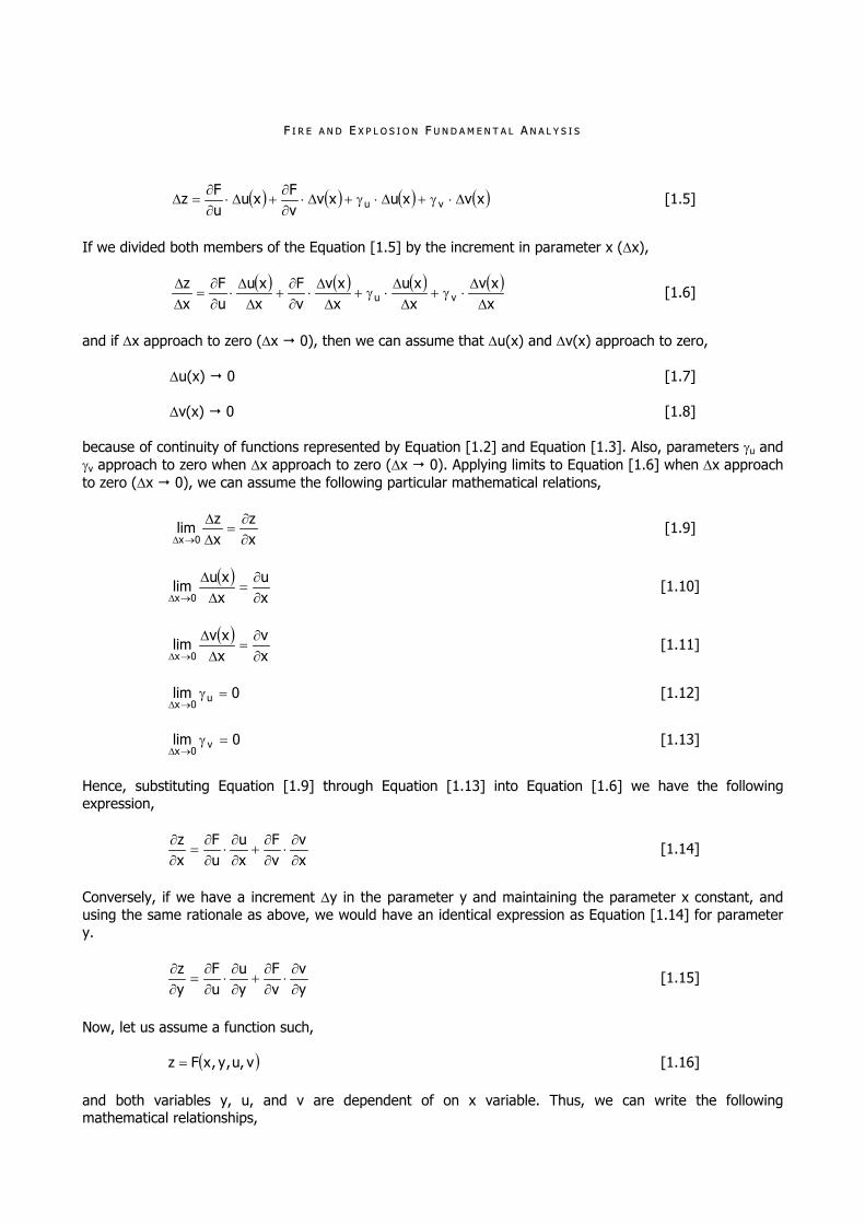
If we divided both members of the Equation [1.5] by the increment in parameter x (x),
xxv
xxu
xxv
vF
xxu
uF
xz
vu
[1.6]
and if x approach to zero (x 0), then we can assume that u(x) and v(x) approach to zero,
u(x) 0 [1.7]
v(x) 0 [1.8] because of continuity of functions represented by Equation [1.2] and Equation [1.3]. Also, parameters u and v approach to zero when x approach to zero (x 0). Applying limits to Equation [1.6] when x approach to zero (x 0), we can assume the following particular mathematical relations,
xz
xz
lim0x
[1.9]
xu
xxu
lim0x
[1.10]
xv
xxv
lim0x
[1.11]
0lim u
0x
[1.12]
0lim v
0x
[1.13]
Hence, substituting Equation [1.9] through Equation [1.13] into Equation [1.6] we have the following expression,
xv
vF
xu
uF
xz
[1.14]
Conversely, if we have a increment y in the parameter y and maintaining the parameter x constant, and using the same rationale as above, we would have an identical expression as Equation [1.14] for parameter y.
yv
vF
yu
uF
yz
[1.15]
Now, let us assume a function such,
v,u,y,xFz [1.16] and both variables y, u, and v are dependent of on x variable. Thus, we can write the following mathematical relationships,

FF II RR EE AA NN DD EE XX PP LL OO SS II OO NN RR II SS KK AA NN AA LL YY SS II SS
xfy [1.17]
xu [1.18]
xv [1.19]
and we can say that Eqation [1.16] is a function of only one variable, the variable x. the derivative can be determined by the following differential equation,
xv
vz
xu
uz
xy
yz
xx
xz
dxdz
[1.20]
The variables y, u, and v are not interdependent but are solely dependent on variable x. In this case, we can consider that the partial derivatives are, in fact, ordinary derivatives,
dxdv
vz
dxdu
uz
dxdy
yz
xz
dxdz
[1.21]
Equation [1.21] is the expression of total derivative function of Equation [1.16]. Let us now consider a domain and a function belonging to that domain (see Figure [1.1]),
z,y,xfu [1.22] and one point in the domain, such M0(x0,y0,z0).
Vector S
z
y
x
M0
M1
s
Figure 1.1 – Schematic of the derivative of an equation in a domain. Consider that we trace one vector S with origin in point M0 and with cosine directors: cos, cos, and cos. Let us assume that over the vector S is a small distance s with origin in point M0 and ending in point M1(x+x, y+y, z+z). Thus, s can be written as,

FF II RR EE AA NN DD EE XX PP LL OO SS II OO NN FF UU NN DD AA MM EE NN TT AA LL AA NN AA LL YY SS II SS
222 zyxs [1.23]
The growing of the function of Equation [1.22] is given by expression,
zyxzzu
yyu
xxu
u zyx
[1.24]
where x, y, and z, are equal to zero when s approachs to zero. Hence, if we divided Equation [1.24] by s then we obtain the following expression identical to Equation [1.6],
sz
sy
sx
sz
zu
sy
vu
sx
xu
su
zyx
[1.25]
Knowing that the cosine directors can be expressed by the following mathematical relations,
sx
cos
[1.26]
sy
cos
[1.27]
sz
cos
[1.28]
the Equation [1.25] can be written as given,
coscoscoscoszu
cosvu
cosxu
su
zyx
[1.29]
The limit of su
when s approach to zero (s 0) is called the derivative of a function in point (x,y,z), and
in the direction of vector S, and it is noted by,
su
su
lim0s
[1.30]
Thus, substituting Equation [1.30] on Equation [1.29] and assuming that when s approach to zero (s 0), parameters x, y, and z, are equal to zero, the Equation [1.29] becomes,
coszu
cosvu
cosxu
su
[1.31]
OO VV EE RR AA LL LL MM AA SS SS BB AA LL AA NN CC EE In fluid dynamics, fluids are in motion. Generally, they are moved from place to place by means of mechanical devices, by gravity, by concentration or temperature gradients, or by pressure. In deriving the general equation for overall mass balance, the law of conservation of mass may be stated as follows for a control volume where no mass is being generated,

FF II RR EE AA NN DD EE XX PP LL OO SS II OO NN RR II SS KK AA NN AA LL YY SS II SS
[rate of mass output] + [rate of mass accumulated] = [rate of mass input] + [rate of mass generated]
[1.32] Considering a control volume fixed in space, as such represented in Figure 1.2, and located in a fluid flow, for a small element of of area, dA, on the control surface, the rate of mass efflux from this element is,
cosdAv [1.33] where the quantity dAcos() is the area projected in the direction normal to the velocity vector (v), is the angle between the velocity vector and the outward-directed unit normal vector (n) to dA, and is the density (kgm3).
v
dA
n
Figure 1.2 – Schematic of a fluid flow for a control volume.
The net mass efflux from control volume is given by,
A
dAcosv [1.34]
We should note that if mass is entering the control volume, i.e. flowing inward across the control surface, the net efflux of mass is negative since < 90º and cos() is negative. The rate of accumulation of mass within the control volume (V) can be expressed as follows,
VdtdM
dVt
[1.35]
where M is the mass (kg) of fluid in the volume (V). substituting Equation [1.33] through Equation [1.35] into Equation [1.32], and assuming the generated mass is null, we can have the following expression for the general form of the overall mass balance.
VA
0dVt
dAcosv [1.36]
For a common situation for a steady state one-dimensional flow, where all flow inward is normal to surface A1 and outward normal to surface A2, as shown in Figure 1.3, the general equation of the overall mass balance is,
12 A
1111A
2222A
dAcosvdAcosvdAcosv [1.37]

FF II RR EE AA NN DD EE XX PP LL OO SS II OO NN FF UU NN DD AA MM EE NN TT AA LL AA NN AA LL YY SS II SS
and
111222A
AvAvdAcosv [1.38]
with 2 being 0º and 1 being 180º. For a steady state,
0dtdM
[1.39]
A2A1
v1, 1 v2, 2
Figure 1.3 – Schematic of a steady state one-dimensional flow.
If the velocity is not constant but varies across the surface area, na average bulk velocity is defined by,
A
avg dAvA1
v [1.40]
for a surface over which the velocity (v) is normal to the surface area (A) and the density () is assumed constant. In obtaining the kinetic energy velocity correction factor () it is necessary to integrate the kinetic energy term,
dAcosv2v
A
2
[1.41]
where is defined as,
avg3
3avg
v
v [1.42]
and
A
3avg
3 dAvA1
v [1.43]
For laminar flow the velocity can be determined by the expression,
2
avg Rr
1v2v [1.44]
and for turbulent flow the velocity is given by,

FF II RR EE AA NN DD EE XX PP LL OO SS II OO NN RR II SS KK AA NN AA LL YY SS II SS
71
max RrR
vv
[1.45]
where r is the radial distance from the center, and R is the area surface equivalent radius.
R
r
Figure 1.4 – Radial distance from the center of a cylinder or sphere. DD II FF FF EE RR EE NN TT II AA LL EE QQ UU AA TT II OO NN SS OO FF CC OO NN TT II NN UU II TT YY AA NN DD MM OO MM EE NN TT UU MM TT RR AA NN SS FF EE RR Various types of time derivatives are used in the dervations to follow. The most common type of derivative is the partial time derivative. The partial time derivative of the function u as described in Equation [1.22] is
tu
. Suppose that we want to measure the function u in the system while we are moving about in the
stream with velocities in the x, y, and z directions of dtdx
, dtdy
, and dtdz
, respectively. The total derivative is
given by mathematical expression,
dtdz
zu
dtdy
vu
dtdx
xu
tu
dtdu
[1.46]
Another useful type of time derivative is obtained if the observer floats along with the velocity (v) of the flowing stream and notes the change in function with respect to time. This is called the substancial time derivative, and is written as follows,
uvtu
vzu
vvu
vxu
tu
DtDu
zyx
[1.47]
where vx, vy, and vz are the velocity components of the stream velocity. For the derivation of the equation of continuity, a mass balance will be made considering a pure fluid flowing through a stationary volume element xyz which is fixed in space (see Figure 1.5). in the x direction the rate of mass entering (kgs1) the face at x having an area (m2) of yz is,
zyv xx [1.48]
and that leaving at x+x is,
zyv xxx [1.49]
The density is denoted by (kgm3), and the term vx is a mass flux (kgs1m2). The rate of accumulation in the volume xyz is,
tzyx
[1.50]

FF II RR EE AA NN DD EE XX PP LL OO SS II OO NN FF UU NN DD AA MM EE NN TT AA LL AA NN AA LL YY SS II SS
z
x
y
(x,y,z)z
x
y
(xx,y,z)
(xx,y,z+z)(x,y,z+z)
(x,y+y,z+z)(x+x,y+y,z+z)
(x+x,y+y,z)(x,y+y,z)
Figure 1.5 – Volume element analysis for equation of continuity. The mass balance for the fluid with a concentration is given by Equation [1.32], and if we substitute the mass balance by Equation [1.48] through Equation [1.50] and also assume that ther is no rate of mass generated, then Equation [1.32] becomes,
tz
vv
y
vv
x
vv zzzzzyyyyyxxxxx
[1.51]
Taking the limit as x, y, andz approach zero, we obtain the equation of continuity or conservation of mass for a pure fluid,
zv
y
v
xv
tzyx [1.52]
We can convert the Equation [1.52] into another form by carrying out the actual partial differentiation,
zv
yv
xv
zv
y
v
xv
t zyxzyx [1.53]
Rearranging Equation [1.53] becomes,
zv
y
v
xv
zv
yv
xv
tzyx
zyx [1.54]
It is often convenient to use cylindrical coordinates. The relation between rectangular coordinates and cylindrical coordinates are as following (see Figure 1.6),
cosrx [1.55]

FF II RR EE AA NN DD EE XX PP LL OO SS II OO NN RR II SS KK AA NN AA LL YY SS II SS
sinry [1.56]
zz [1.57]
22 yxr [1.58]
xy
tan 1 [1.59]
For spherical coordinates the variables r, , and are related to rectangular coordinates by the following expression as shown,
cossinrx [1.60]
cossinry [1.61]
cosrz [1.62]
222 zyxr [1.63]
zyx
tan22
1 [1.64]
xy
tan 1 [1.65]
z
x
(x,y,z)
r
y
z
x
(x,y,z)
r
y
Cylindrical Coordinates Spherical Coordinates
Figure 1.6 – Relation between rectangular, cylindrical, and spherical coordinates.
FF II RR EE AA NN DD EE XX PP LL OO SS II OO NN FF UU NN DD AA MM EE NN TT AA LL AA NN AA LL YY SS II SS
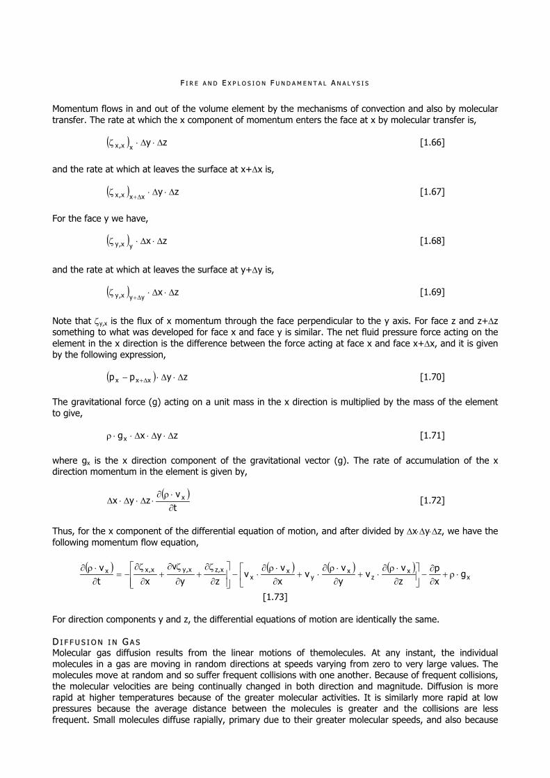
Momentum flows in and out of the volume element by the mechanisms of convection and also by molecular transfer. The rate at which the x component of momentum enters the face at x by molecular transfer is,
zyxx,x [1.66]
and the rate at which at leaves the surface at x+x is,
zyxxx,x
[1.67]
For the face y we have,
zxyx,y [1.68]
and the rate at which at leaves the surface at y+y is,
zxyyx,y
[1.69]
Note that y,x is the flux of x momentum through the face perpendicular to the y axis. For face z and z+z something to what was developed for face x and face y is similar. The net fluid pressure force acting on the element in the x direction is the difference between the force acting at face x and face x+x, and it is given by the following expression,
zypp xxx [1.70] The gravitational force (g) acting on a unit mass in the x direction is multiplied by the mass of the element to give,
zyxgx [1.71] where gx is the x direction component of the gravitational vector (g). The rate of accumulation of the x direction momentum in the element is given by,
tv
zyx x
[1.72]
Thus, for the x component of the differential equation of motion, and after divided by xyz, we have the following momentum flow equation,
x
xz
xy
xx
x,zx,yx,xx gxp
zv
vyv
vxv
vzy
v
xtv
[1.73]
For direction components y and z, the differential equations of motion are identically the same. DD II FF FF UU SS II OO NN II NN GG AA SS Molecular gas diffusion results from the linear motions of themolecules. At any instant, the individual molecules in a gas are moving in random directions at speeds varying from zero to very large values. The molecules move at random and so suffer frequent collisions with one another. Because of frequent collisions, the molecular velocities are being continually changed in both direction and magnitude. Diffusion is more rapid at higher temperatures because of the greater molecular activities. It is similarly more rapid at low pressures because the average distance between the molecules is greater and the collisions are less frequent. Small molecules diffuse rapially, primary due to their greater molecular speeds, and also because

FF II RR EE AA NN DD EE XX PP LL OO SS II OO NN RR II SS KK AA NN AA LL YY SS II SS
the chance for collisions is not so great as for large olecules. Thus, in general, diffusion increases with an increase in molecular weight and the size of the individual molecule. Using Fick’s law as the fundamental relationship, many of the standard molecular diffusion equations may be derived. The Fick’s law states the dependence of diffusional flow on concentration gradient, and is defined by the equation,
dtdzdC
ADdn [1.74]
namely, that dn is the quantity of material diffusing in z direction, through an area (A), proportional to the
time interval (dt), the area and the concentration gradient (dC) in the direction of diffusion dzdC
. The
proportionality factor (D) is the diffusivity,or diffusion coefficient, of te soute material through the bulk fluid. The Fick’s law is the fundamental equation of diffusion, andit was developed from the kineic theory of gases. Ulike the rate of transfer,the amount of material transferred across the interfaceis not dependent on the concentration gradient, but rather on the equilibrium relationship. Equilibrium conitions will establish the maximum amount of material which can be transferred, while the concentratin gradient driving force will determine how fast the material will be transferred. It is also common practice to assume that the deal gas law is applicable,
TRnVp [1.75] where V is the total volume (m3), ni is the quantity (moles of component), pi is the partial pressure (atm), T is the temperature (K), and R is the ideal gas constant (82.07 cm3atmg-mole1K1). Furthermore, the concentration canbe expressed by,
TRp
Vn
C iii
[1.76]
and
Pp
y ii [1.77]
where yi is the fraction of a compoent in a gas mixture, and P is the total pressure of a system of gases. The rate of diffusion per unit area of a gas component is given by,
zCTRC
PDnLN
i
[1.78]
where z is the path of diffusion or the distance between the two points of concentration, and C is the difference of concentration (concentration gradient) between two points, and is determined by the following equation,
1
2
12LN
CC
LN
CCC [1.79]
For gases, the concentration is equivalent to the partial pressure and can be determined by the Equation [1.76]. The gas diffusivity (diffusion coefficient) is a property of the system, and is dependent on the temperature, pressure, and nature of the components or substances. The diffusion coefficient (D), in units cm2s1, at a given temperature (T) and pressure (P) may be determined by the following expression,

FF II RR EE AA NN DD EE XX PP LL OO SS II OO NN FF UU NN DD AA MM EE NN TT AA LL AA NN AA LL YY SS II SS
P1
T15.273T15.273
DDb
00
[1.80]
where T0 is temperature at initial conditions (ºC), P is the total pressure of the system (atm), and b is a temperature coefficient. Table 1.1 presents a list diffusion coefficients for some pairs of gases.
Table 1.1 – Values of diffusion coefficients of gases at atmospheric pressure.
DD00 TT00 GGaass oorr VVaappoorr ((ccmm22//ss))
SSyysstteemm ((ººCC))
bb
Methane 0.1960 0 1.75 Chloride 0.1238 20 1.00 Carbon dioxide 0.1380 0 2.00 Hydrogen 0.6110 0 1.75 Water (vapor) 0.2200 0 1.75 Methanol 0.1325 0 1.75 Ethanol 0.1020 0 2.00 Propanol 0.0850 0 2.00 Naphthalene 0.0513 0 2.00 Butanol 0.0727 0 2.00 n-hexane 0.0800 21 Benzene 0.0770 1.75 Toluene 0.0710 2.00 o-xylene 0.0620 1.75 p-xylene 0.0560 2.00 m-xylene 0.0590 1.75 Anthracene 0.0421 2.00 NH3 0.2270
Air
0
PP RR II NN CC II PP LL EE SS OO FF SS TT EE AA DD YY SS TT AA TT EE HH EE AA TT TT RR AA NN SS FF EE RR The transfer of energy in the form of heat occurs in many chemical and other types of processes. The heat transfer occurs because of a temperature difference driving force and heat flows from the high to low temperature region. Writing a similar equation to balance of momentum, but specifically for thermal energy transfer,
[input rate of heat]+[rate of heat generated] = [output rate of heat] + [rate of heat accumulated]
[1.81] and making an unsteady state heat balance for the x direction only on the element of volume (control volume), in Figure 1.7, and with the cross-sectional area being A (m2), we have the following differential thermal equation,
AxtT
cqAxqq pxxGx [1.82]
where qG is the rate of heat generated per unit volume, qx is the rate of heat entering the element of volume in the x direction, and qx+x is the rate of heat leaving the element of volume in the x direction. Heat transfer may occur by any one or more of the three basic mechanisms of hat transfer: conduction, convection, and radiation.

FF II RR EE AA NN DD EE XX PP LL OO SS II OO NN RR II SS KK AA NN AA LL YY SS II SS
qx qx+x
x x+x
x
Figure 1.7 – Heat transfer in the x direction on an element volume.
HH EE AA TT CC OO NN DD UU CC TT II OO NN TT RR AA NN SS FF EE RR Heat is conducted through solids, liquids, and gases, by the transfer of energy of motion between adjacent molecules, and in which a temperature gradient exists. Hence, heat transfer by conduction is dependent upon the driving force of temperature difference and the resistance to heat transfer. The resistance to heat transfer is dependent upon the nature and dimensions of the heat transfer medium. All heat transfer problems involve the temperature difference, the geometry, and the physical properties of the object being studied. In conduction, energy can also be transferred by «free» electrons. In conduction heat transfer, the most common means of correlation is through Fourier’s law of conduction,
dxdT
kAqx [1.83]
where qx is the heat transfer rate in the x direction (W), A is the cross-sectional area normal to the direction of flow of heat (m2), T is absolute temperature (K), x is the distance (m), and k is the thermal conductivity
(Wm1K1). The quantity Aqx is called the heat flux (Wm2). Rearranging Equation [1.83] and integrating,
assuming that the thermal conductivity (k) is constant and does not vary with temperature, we have the following expression,
2
1
2
1
T
T
x
x
x dTkdxAq
[1.84]
Simplifying Equation [1.84] becomes,
12
21x
xxTT
kAq
[1.85]
For gases, thermal conductivity increases approximately as the square root of the absolute temperature and is independent of pressure up to a few atmospheres. At very low pressures (vacuum) however, the thermal conductivity approaches zero. The thermal conductivity of liquids varies moderately with temperature and often can be expressed as a linear variation,
Tbak [1.86]
Table 1.2 – Values of diffusion coefficients of gases at atmospheric pressure.
kk TT kk TT SSuubbssttaannccee ((WW//mmKK)) ((KK))
SSuubbssttaannccee ((WW//mmKK)) ((KK))
0.0242 273.15 0.1590 303.00 Air 0.0316 373.15
Benzene 0.1510 333.00
0.5690 273.15 n-butane 0.0135 273.15 Water 0.6800 366.00 Hydrogen 0.167 273.15

FF II RR EE AA NN DD EE XX PP LL OO SS II OO NN FF UU NN DD AA MM EE NN TT AA LL AA NN AA LL YY SS II SS
CC OO NN VV EE CC TT II VV EE HH EE AA TT TT RR AA NN SS FF EE RR The transfer of heat by convection implies the transfer of heat by bulk transport and mixing of macroscopic elements of warmer portions with cooler portions of a gas or a liquid, and also often involves the energy exchange between a solid surface and a fluid by a density difference resulting from the temperature differences in the fluid. The term natural convection is used if this motion and mixing is caused by density variations resulting from temperature differences within the fluid. The term forced convection is used if this motion and mixing is caused by an outside force. Heat transfer by convection is more difficult to analyze than heat transfer by conduction because no single property of the heat transfer medium, such as thermal conductivity, can be defined to describe the mechanism. Heat transfer by convection varies from situation to situation (upon the fluid flow conditions), and it is frequently coupled with the mode of fluid flow. In practice, analysis of heat transfer by convection is treated empirically (by direct observation). We express the rate of heat transfer from the fluid to the surface (interface), or vice versa, by the following equation,
fsc TTAhq [1.87] where q is the heat transfer rate (W), A is the area (m2), Ts is the temperature of the surface (K), Tf is the average or bulk temperature (K) of the fluid flowing by, and hc is the convective heat transfer coefficient (Wm2K1). The convective heat transfer coefficient (hc) is a finction of the system geometry, fluid properties, flow velocity, and temperature difference (temperature gradient). To convert the convective heat transfer coefficient from English units to Standard International units we must use the following relation,
1 Btuhr1ft2 = 5.6783 Wm2K1 [1.88] In Table 1.3 some order-of-magnitude values of convective heat transfer coefficient for diferent convective mechanisms of free or natural convection, forced convection, boiling, and condensation are given.
Table 1.3 – Approximate magnitude of some heat transfer coefficients.
hhcc MMeecchhaanniissmm ((WW//mmKK))
Condensing steam 5,700 – 28,000 Condensing organics 1,100 – 2,800 Boiling liquids 1,700 – 28,000 Moving water 280 – 17,000 Moving hydrocarbons 55 – 1,700 Still air 3 – 1,700 Moving air 11 – 55
Heat conduction through a hollow sphere, using Fourier’s law for constant thermal conductivity with distance gap (dr), where r is the radius of the sphere, and the cross-sectional area normal to the heat flow is,
2r4A [1.89] Substituting Equation [1.89] into Equation [1.83] and rearranging,
drdT
kr4
q2
[1.90]
and integrating Equation [1.90] becomes,
2
1
2
1
T
T
r
r2
dTk4drr
1q [1.91]
Simplifying the Equation [1.91] becomes,

FF II RR EE AA NN DD EE XX PP LL OO SS II OO NN RR II SS KK AA NN AA LL YY SS II SS
12
2121 rr
TTrrk4q [1.92]
II NN TT EE RR NN AA LL HH EE AA TT GG EE NN EE RR AA TT II OO NN In certain systems heat is generated inside the conducting medium, i.e. a uniformly distributed heat source is present. Also, if a chemical reaction is occuring uniformly in a medium, a heat of reaction is given off. Heat is conducted in x, y, and z directions. The temperature at x, y, and z directions is held constant. The volumetric rate of heat generation is denoted by qG (Wm3), and the thermal conductivity of the medium is denoted by k (Wm1K1). To derive the mathematical equation for this case of heat generation at steady state, we start with the following heat balance expression,
xxGx qAxqq [1.93] and the heat accumulated is null, where A is the cross-sectional area. Rearranging, dividing by x, and letting x approach zero, we have the following expression,
0Aqx
qqG
xxx
[1.94]
or
0Aqdx
dqG
x [1.95]
Substituting Equation [1.83] becomes,
0k
q
dx
Td G2
2 [1.96]
Integration of Equation [1.96] gves the following solution,
212 cxcx
k2q
T
[1.97]
where c1 and c2 are integration constants. At initial limits when x = 0, and T = T0 (T0 is the source heat generation temperature), the constant c2 becomes,
x = 0 c2 = T0 [1.98] and at final limits when x = L, and T = Ts (Ts is the temperature at the distance point from source heat generation), the temperature profile is given by expression,
012
s TLcLk2
qT
[1.99]
Simplifying Equation [1.99] and solving to constant c1,
2
0s1 Lk2
qTT
L1
c [1.100]
and substituting into Equation [1.97] gives,

FF II RR EE AA NN DD EE XX PP LL OO SS II OO NN FF UU NN DD AA MM EE NN TT AA LL AA NN AA LL YY SS II SS
L1
1TLT
Lxk2
qT 0
s2 [1.101]
which is the temperature profile for a given point (x) between heat generation source and a given distance (L) from the source heat generation. VV OO LL UU MM EE TT RR II CC CC OO EE FF FF II CC II EE NN TT OO FF EE XX PP AA NN SS II OO NN Density differences in the fluid arising from the heating process provide the buoyancy force required to move the fluid. The density difference can be expressed in terms of the volumetric coefficient of expansion (). For gases, the volumeric coefficient expansion is given by,
T1
[1.102]
or, more precisely by expression,
b
b
TT
[1.103]
where Tb is the bulk temperature (K), T is the temperature predicted (K), is the density for the predicted temperature, and b is the density for bulk temperature. RR AA DD II AA TT II OO NN HH EE AA TT TT RR AA NN SS FF EE RR In radiation heat transfer no physical medium is needed for its propagation. Radiation is the transfer of energy through space by means of elctromagnetic waves in much the same way as electromagnetic light waves transfer light. Most energy of this type is in the infrared region of the electromagnetic spectrum although some of it is in the visible region. The same laws which govern the transfer of light govern the radiant transfer of heat. Solids and liquids tend to absorb the radiation being transferred through it, so that radiation is important primarily in transfer through space or gases. Any material that has a temperature above absolute zero gives off some radiant energy. The exchange of radiation between two surfaces depends upon the size, shape, and relative orientation of these two surfaces and also upon their emissivities and absorptivities. In cases to be considered the surfaces are separated by nonabsorbing media such as air. When gases such carbon dioxide (CO2) and water vapor are preent, some absorption by the gases or vapors occurs. Radiation Spectrum and Thermal Radiation Energy can be transported in the form of electromagnetic waves and these waves travel at the speed of light. Bodies may emit many forms of radiation energy, such gamma rays, thermal energy, radio waves, and so on. In fact there is a continuous spectrum of electromagnetic radiation. This electromagnetic spectrum is divided into a number of wave length ranges such as cosmic rays ( < 1013 m), gamma rays (1013 m < < 1010 m), thermal radiation (107 m < < 104 m), and so on. The electromagnetic radiation produced solely because of temperature of the emitter is called thermal radiation and exists between the wavelengths of 107 m and 104 m. electromagnetic waves having wavelengths between 3.8107 m and 7.6107 m, called visible radiation, can be detected by the human eye. When different suraces are heated to the same temperature, they do not all emit or absorb the source amount of thermal radiant energy. A body that absorbs and emits the maximum amount of energy at a given temperature is called a black body – a standard to which other bodies can be compared. When a black body is heated to a given temperature, photons are emitted from the surface which have a definite distribution of energy. Planck’s equation relates the monochromatic emissive power (EB,), in Wm3 units, at a absolute temperature (T), in Kelvin (K) degree units, and a wavelength (), in metric units,

FF II RR EE AA NN DD EE XX PP LL OO SS II OO NN RR II SS KK AA NN AA LL YY SS II SS
1T104388.1
exp
107418.3E
25
16
,B [1.104]
Also, for a given temperature, the emissive power reaches a maximum value at a wavelength that decreases as the absolute temperature increases. For a given temperature, the wavelength at which a black body emissive power is a maximum can be determined by differentiating Equation [1.104] with respect to wavelength () at constant temperature and setting the result equal to zero. The result is known as Wien’s displacement law,
3max 10898.2T [1.105]
The total emissive power is the total amount of radiation per unit area leaving a surface with temperature over all wavelengths. For a black body, the total emissive power (Wm2) is given by,
0
,BB dEE [1.106]
and solving the integral gives,
4B TE [1.107]
The result is the Stephan-Boltzmann law with = 5.676108 Wm2K. An important property in radiation is the emissivity () of a surface and is defined as the total emitted energy of the surface divided by the total emitted energy of a black body at the same temperature.
4B T
EEE
[1.108]
The Kirchhoff’s law states that at thermal equilibrium the absorptivity (a) is equal to the emissivity () of a body,
B
a EE
[1.109]
When a body is not at equilibrium with its surroundings, the reslt is not valid. The absorptivity of a surface actually varies with the wavelength of the incident radiation. The absorptivity (a) is assumed constant even with a variation in the wavelength of the incident radiation. Also, in actual systems, various surfaces may be at different temperatures, and the absorptivity for a surface is evaluated by determining the emissivity at the temperature of the source of the other radiating surface or emitter since this is the temperature the absorbing surface would reach if the absorber and emitter were at thermal equilibrium. The temperature of the absorber has only a slight effect on the absorptivity. View Factors in Radiation If two surfaces are arranged so that radiant energy can bexchanged, a net flow of energy will occur from the hotter surface to the colder surface. The size, shape, and orientation of two radiating surfaces or a system of surfaces are factors in determining the net heat flow rate between them. If two parallel and infinite black surface planes, surface A1 and surface A2, at temperature T1 and T2, respectively, are radiating toward each other, surface A1 emits radiation,

FF II RR EE AA NN DD EE XX PP LL OO SS II OO NN FF UU NN DD AA MM EE NN TT AA LL AA NN AA LL YY SS II SS
411 TE [1.110]
to surface A2, which is also absorbed. Also, surface A2 emits radiation,
422 TE [1.111]
to surface A1, which is also absorbed. Then for surface A1, the net radiation (q12) is from surface A1 to surface A2, with a fraction (F12) of radiation leaving surface A1 that is intercepted by surface A2,
42
4111212 TTAFq [1.112]
The factor F12 is called the geometric view factor. Hence, for surface A2, the net radiation (q21) that is transferred is given by,
42
4122112 TTAFq [1.113]
In the case of parallel surfaces, F12 = F21 = 1.0, and the geometric factor is simply omitted. F12 is the fraction of radiation leaving surface A1 in all directions, and which is intercepted by surface A2. F21 is the fraction of radiation leaving surface A2 in all directions, and which is intercepted by surface A1. If both of the parallel surfaces (A1 and A2) are gray bodies with emissivities and absorptivities of 1 = 1 and 2 = 2, respectively, the radiation energy absorbed by surface A2 is,
41112 TA [1.114]
and the radiation relected by surface A2 is the fraction,
41112 TA1 [1.115]
The net radiation transferred by surface A1 is given by,
111
TTAq
21
42
41
112 [1.116]
If we insert one or more radiation surfaces between the original surfaces,
1
2TT
1n1
Aq42
41
n12 [1.117]
where n is the number of radiation surfaces or shields between original surfaces, and is the emissivity. Hence, a great reduction in radiation heat loss is obtained by using these shields. Suppose that we consider radiation between two parallel black surfaces of finite size like those represented in Figure 1.8. Since the surfaces are not infinite in size, some of the radiation from surface A1 does not strike surface A2, and vice versa. Hence, the net radiation interchange is less since some is lost to the surroundings. In the Figure 1.8, the differential solid angle (d), a solid angle is a dimensionless quantity which is a measure of an angle in solid geometry, is equal to the normal projection of dA2 divided by the square of the distance between the point P and area dA2.

FF II RR EE AA NN DD EE XX PP LL OO SS II OO NN RR II SS KK AA NN AA LL YY SS II SS
2
22
r
cosdAd
[1.118]
The intensity of radiation for a black body (IB) is the rate of radiation emitted per unit area projected in a direction normal to the surface and per unit solid angle (steradin, sr) in a specified direction.
dcosdAdq
I1
B [1.119]
and IB is in Wm1sr1 units. The emissive power (EB) which leaves a black body plane surface is determined by integrating Equation [1.119] over all solid angles subtended by a hemisphere covering the surface.
BB IE [1.120] where EB is in Wm2 units.
dA2
d
r
IB
P
d
dA1
Figure 1.8 – Heat radiation transfer between two finite parallel black surfaces. The rate of radiant energy that leaves dA1 in the direction given by the angle 1 is,
111,B cosdAI [1.121]
The rate of radiant energy that leaves dA1 and arves on dA2 is given by,
dcosdAIdq 111,B21 [1.122]
where d is the solid angle subtended by the area dA2 as seen from dA1. Combining Equation [1.118] through Equation [1.222] we have the following expression,
2
21211,B21
r
dAdAcoscosEdq
[1.123]
The radiant energy leaving dA2 and arriving at dA1 is given by,

FF II RR EE AA NN DD EE XX PP LL OO SS II OO NN FF UU NN DD AA MM EE NN TT AA LL AA NN AA LL YY SS II SS
221211,B
12r
dAdAcoscosEdq
[1.124]
Taking the difference of Equation [1.123] and Equation [1.124],
221214
24112
r
dAdAcoscosTTdq [1.125]
Performing the double integration over surfaces A1 and A2 will yield the total net heat flow between the finite areas.
2 1A A2
212142
4112
r
dAdAcoscosTTdq [1.126]
dA2
dA1
r
N1
N2
Figure 1.9 – Heat radiation transfer between two finite black surfaces.
Equation [1.126] can also be written as,
42
41221
42
4111212 TTAFTTAFq [1.127]
Also, the following relation exists,
212121 FAFA [1.128] The view factor is then,
2 1A A2
2121
j,ij,i
r
dAdAcoscosA1
F [1.128]
Values of the view factor can be calculated for a number of geometrical arrangements. The view factor from a plane to a hemisphere can be interpreted as being represented by Fgure 1.10. since surface A1 sees only surface A2, the view factor F12 is 1.0. using Equation [1.128] we can establish the relationship between F12 and F21,
21212
2
211
212 F2F
r
r2F
AA
F
[1.129]
Hence,

FF II RR EE AA NN DD EE XX PP LL OO SS II OO NN RR II SS KK AA NN AA LL YY SS II SS
21
0.121
F21
F 1221 [1.130]
Because,
1FF 2221 [1.131] and substituting the relation resulted from Equation [1.130] in Equation [1.131] we have the following,
21
21
1F22 [1.132]
L
A1
A2
d
d
d=d d sin
Figure 1.10 – Heat radiation transfer between a flat finite black surface and a hemisphere black surface.
Radiation in Absorbing Gases Most gases that are mono-atomic or diatomic, such as He, Ar, H2, O2, and N2, are virtually transparent to thermal radiation, i.e. they emit practically no radiation and also do no absorb radiation. Gases with a dipole moment and higher polyatomic gases emit significant amounts of radiation and also absorb radiant energy eithin the same bands in which they emit radiation. These gases include carbon dioxide (CO2), water vapor, carbon monoxide (CO), sulphur dioxide (SO2), NH3 ,and organic vapors. For a particular gas, the width of the absorption or emission bands depends on the pressure and also the temperature. The absorption of radiation in a gas layer can be described analytically since the absorption by a given gas depends on the number of molecules in the path of radiation. Increasing the partial pressure of the absorbing gas or the path length increases the amount of absorption. If a beam impinges on a gas layer of thickness (dL), the decrease in intensity (dI) is proportional to the intensity (I) and gas layer thickness (dL).
dLIdI ,a [1.133]
Integrating Equation [1.133] becomes,
L,a
0eII
[1.134]
The constant a, depends on the particular gas, its partial pressure, and the wavelength of radiation. This equation is called Beer’s law. Thick layers of a gas absorb more energy than do thin layers. For a black differential receiving surface area (dA) located in te center of the base of a hemisphere of radius (L) containing a radiant gas, the mean beam length is L. The mean beam length has been evaluated for various geometries is given in Table 1.4. For other shapes, the mean beam length (L) can be aroximated by the following relation between gas volume (V) and surface area (A) of the enclosure,
AV
6.3L [1.135]

FF II RR EE AA NN DD EE XX PP LL OO SS II OO NN FF UU NN DD AA MM EE NN TT AA LL AA NN AA LL YY SS II SS
where volume is given in m3 units, and the surface area is in m2 units. Gas emissivity (G) is defined as the ratio o the rate of energy transfer from the hemispherical body of gas to a surface element t the midpoint divided by the rate of energy transfer from a black hemisphere surface of radius (L) and temperature (TG) to the same element.
Table 1.4 – Mean beam length (L) for gas radiations to entire enclosure surface.
MMeeaann BBeeaamm LLeennggtthh GGeeoommeettrryy ((mm))
Sphere, diameter (D) 0.65D Infinite cylinder, diameter (D) 0.95D Cylinder, length = diameter (D) 0.60D Infinite parallel plates, separation distance (D) 1.80D Hmisphere, radius (R) R Cube, side length (D) 0.60D Volume surrounding bank of long tubes with centers on equilateral triangle, tube diameter (D) = clearence 2.80D
The rate of radiation emitted from the gas is given by,
4GG T [1.136]
of receiving surface element, where the gas emissivity (G) is evaluated at gas temperature (TG). the net rate of radiant transfer between a gas at TG and a black surface of finite area (A) at a given temperature (T1) is then,
41G
4GG TTAq [1.137]
where G is the absorptivity of the gas for a black body radiation from the surface at temperature T1. for the case where the walls of the enclosure are not black, some of the radiation striking the walls is reflected back to the other walls and into the gas. As an approximation when the emissivity of the walls is greater than 0.7, an effective eissivity (ef) can be used,
21 ef
[1.138]
where is the actual emissivity of the enclosure walls. Then Equation [1.137] is modified,
41G
4GGef TTAq [1.139]
The case of radiation between parallel disks where we have a small disk of area A1 parallel to a large disk of area A2, and both centered directly with each other, is shown in Figure 1.11. The distance between the centers of the disks is denoted by R. From the geometry shown by Figure 1.11,
222 xRr [1.140] and
22
1xR
Rcos
[1.141]
The differential area for disk A2 is taken as the circular ring of radius x so that,

FF II RR EE AA NN DD EE XX PP LL OO SS II OO NN RR II SS KK AA NN AA LL YY SS II SS
dxx2dA2 [1.142]
A2
r
A1
R
ax
Figure 1.11 – Heat radiation transfer between two centered parallel disks of different dimensions. Using Equation [1.128] and substituting dA2 by Equation [1.142] becomes,
2 1A A2
121
112
r
dxx2dAcoscosA1
F [1.143]
Solving Equation [1.143] and simplifying,
22
2a
0222
2
12aR
adx
xR
xR2F
[1.144]
PP RR II NN CC II PP LL EE SS OO FF UU NN SS TT EE AA DD YY SS TT AA TT EE HH EE AA TT TT RR AA NN SS FF EE RR Before steady state conditions can be reached in a process, some time must elapse after the heat transfer process is initiated t allow th unstaeady state conditions to disappear. To derive the equation for unsteady state cndition in one direction in a solid, we refer to Figure 1.7. UU NN SS TT EE DD YY SS TT AA TT EE HH EE AA TT CC OO NN DD UU CC TT II OO NN TT RR AA NN SS FF EE RR Heat is being conducted in the x direction in the volume xyz in size. For a conduction in the x direction we can use one similar equation to Equation [1.83],
xT
kAqx
[1.145]
The term xT
means the partial or derivative of temperature (T) with respect to x direction, and other
variables such y and z directions, and time (t) being held constant. Making a balance on the volume element, the rate of heat input is given by,
xx x
Tzykq
[1.146]
FF II RR EE AA NN DD EE XX PP LL OO SS II OO NN FF UU NN DD AA MM EE NN TT AA LL AA NN AA LL YY SS II SS
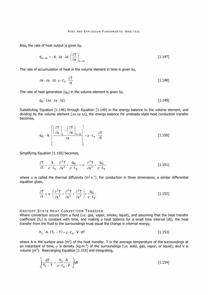
Also, the rate of heat output is given by,
xxxx x
Tzykq
[1.147]
The rate of accumulation of heat in the volume element in time is given by,
tT
czyx p [1.148]
The rate of heat generation (qG) in the volume element is given by,
zyxqG [1.149] Substituting Equation [1.146] through Equation [1.149] in the energy balance to the volume element, and dividing by the volume element (xyz), the energy balance for unsteady state heat conduction transfer becomes,
tT
cx
xT
xT
kq pxxx
G
[1.150]
Simplifying Equation [1.150] becomes,
p
G2
2
p
G2
2
p cq
x
Tc
q
x
Tck
tT
[1.151]
where is called the thermal diffusivity (m2s1). For conduction in three dimensions, a similar differential equation gives,
p
G2
2
2
2
2
2
cq
z
T
y
T
x
TtT
[1.152]
UU NN SS TT EE DD YY SS TT AA TT EE HH EE AA TT CC OO NN VV EE CC TT II OO NN TT RR AA NN SS FF EE RR Where convection occurs from a fluid (i.e. gas, vapor, smoke, liquid), and assuming that the heat transfer coefficient (hc) is constant with time, and making a heat balance for a small time interval (dt), the heat transfer from the fluid to the surroundings must equal the change in internal energy,
dTVcTTAh pfc [1.153]
where A is the surface area (m2) of the heat transfer, T is the average temperature of the surroundings at an instantant of time, is density (kgm3) of the surroundings (i.e. solid, gas, vapor, or liquid), and V is volume (m3). Rearranging Equation [1.153] and integrating,
T
T
t
0p
c
f0
dtVc
AhTT
dT [1.154]

FF II RR EE AA NN DD EE XX PP LL OO SS II OO NN RR II SS KK AA NN AA LL YY SS II SS
Simplifying Equation [1.154] becomes,
tVc
Ah
0
f p
c
eTTTT
[1.155]
This equation describes the time-tempearture history. At any time, the instantaneous rate of heat transfer, neglecting internal resistances, can be calculated from equation,
fc TTAhtq [1.156] Substituting the instantaneous temperature from Equation [1.155] into Equation [1.156] becomes,
t
VcAh
fcp
c
eTTAhtq
[1.157] To determine the total amount of heat (Q) transferred, wecan integrate Equation [1.157],
t
VcAh
f0p
t
0
p
c
e1TTVcdttqQ [1.158]
UU NN SS TT EE DD YY SS TT AA TT EE HH EE AA TT RR AA DD II AA TT II OO NN TT RR AA NN SS FF EE RR Like convection heat transfer, we assume that the heat transfer is constant with time. Making a heat balance for a small time interval (dt), the heat transfer from the fluid (i.e. gas, vapor, smoke, liquid) to the surroundings must equal the change in internal energy,
dTVcTTAF p4
f4ffef [1.159]
where F is view factor, ef is the effective emissivity, f is the fluid emissivity, f is the fluid absorptivity, A is the surface area (m2) of the heat transfer, Tf is the average temperature of the fluid at an instantant of time, T is the average temperature of the surroundings at an instantant of time, is density (kgm3) of the surroundings (i.e. solid, gas, vapor, or liquid), and V is volume (m3). Rearranging Equation [1.159] and integrating,
T
T
t
0p
ef4
f4ff0
dtVc
AF
TT
dT [1.160]
gives the solution,
tVc
AF
TT
TT
LNT
T
tanT2 p
ef
25.0f
f
ff
25.0f
25.0f
f
ff
25.0f
f75.0
f
f
f75.0f
13f
25.1f
f
f25.0f
[1.161] Simplifying Equation [1.161] becomes,

FF II RR EE AA NN DD EE XX PP LL OO SS II OO NN FF UU NN DD AA MM EE NN TT AA LL AA NN AA LL YY SS II SS
tT
VcAF
2
TT
TT
LNT
T
tan
f
f25.0f
3f
25.1f
p
ef
25.0f
f
ff
25.0f
25.0f
f
ff
25.0f
f75.0
f
f
f75.0f
1
[1.162] This equation describes the time-tempearture history. At any time, the instantaneous rate of heat transfer, neglecting internal resistances, can be calculated from equation,
4f
4ffef TTAFtq [1.163]
Substituting the instantaneous temperature (T) obtained from Equation [1.162] into Equation [1.163] and integrating gives the total amount of heat (Q) transferred,
dttqQt
0
[1.164]
Table 1.5 – Normal total emissivities () of several surfaces.
TTeemmppeerraattuurree TTeemmppeerraattuurree SSuurrffaaccee ((KK))
EEmmiissssiivviittyy (()) SSuurrffaaccee ((KK))
EEmmiissssiivviittyy (())
Aluminium 366 0.200 Rubber (hard) 298 0.940 Aluminium (oxidized) 500 0.039 Rubber (glossy) 296 0.940 Aluminium (polished) 850 0.057 Concrete (rough) 313 0.940 Aluminium (oxide) 550 0.630 Paint 373 0.920 – 0.960 Iron (oxidized) 373 0.740 Water 273 0.950 Iron (tin-plated) 373 0.070 373 0.963 Iron (oxide) 772 0.850 Snow 283 0.820 Copper (oxidized) 298 0.780 293 0.820 Copper (polished) 390 0.023 Quartz 373 0.890 Nickel (oxidized) 373 0.072 1273 0.580 Nickel (oxide) 922 0.590 Paper (white) 313 0.950 – 0.980 Steel (stainless) 373 0.074 Paper (colored) 313 0.920 – 0.940 Steel (304 stainless) 489 0.440 Glass (pyrex) 533 0.940 Iron (rusted) 313 0.610 – 0.850 813 0.740 Iron (wrough, dull) 293 – 633 0.940 Glass (smooth) 295 0.940 Brass 520 0.028 Glass (quartz) 533 0.960 630 0.031 813 0.660 Tin 363 0.05 Plaster 313 0.920 Tungstan 513 0.110 533 0.920 1363 0.160 Wood 313 0.800 – 0.900 3033 0.390 Ice 273 0.980
In practice, the amount of heat transferred is measured by the following expression,
t100T
100T
cFtQ4
24
1i
[1.165]
where F is the view factor for radiation source surface, ci is radiation coefficients (kJm2h1K4), T1 is the average or bulk temperature (K) of the radiation source surface, T2 is the average or bulk temperature (K) of

FF II RR EE AA NN DD EE XX PP LL OO SS II OO NN RR II SS KK AA NN AA LL YY SS II SS
the surface that receives radiation, and t is time. For some materials the radiation coefficients (ci) are presented in Table 1.6.
Table 1.6 – Radiation coefficients for some materials.
ccii MMaatteerriiaall ((kkJJ//mm22hhKK44))
Silver (polished) 0.419 Aluminium (polished) 0.837 Dark surfaces 16.747 Glossy surfaces 12.560 Glass, porcelain, varnish 19.259 Wood 19.259 White surfaces 20.725
CC OO MM BB UU SS TT II OO NN AA NN DD SS MM OO KK EE The term “smoke” is defined as the smoke aerosol or condensed phase component of the products of combustion and includes the evolved gases as well (American Society for Testing and Materials, ASTM). Smoke aerosols vary widely in appearance and structure, from light colored, for droplets produced during smoldering combustion and fuel pyrolysis, to black, for solid, carbonaceous particulate or soot produced during flaming combustion. A large fraction of the radiant energy emitted from a fire results from the black body emission from the soot in the flame. The subject of radiant heat transfer is of such importance that it was treated elsewhere. Here we have an focus on smoke aerosols outside the combustion zone. The effects of the smoke produced by a fire depend on the amount of smoke produced and on the properties of the smoke. The smoke emission, together with the flow pattern, determines the smoke concentration as smoke moves throughout a space. The most basic physical property of smoke is the size distribution of its particles. SS MM OO KK EE PP RR OO DD UU CC TT II OO NN Smoke emission is one of the basic elements for characterizing a fire environment. The combustion conditions under which smoke is produced – flaming, pyrolysis, and smoldering – affect the amount and character of the smoke. The smoke emission from a flame represents a balance between growth processes in the fuel-rich portion of the flame and burnout with oxygen (see Figure 1.12). While it is not possible at the present time to predict the smoke emission as a function of fuel chemistry and combustion conditions, it is known that an aromatic polymer, such as polystyrene, produces more smoke than hydrocarbons with single carbon-to-carbon bonds, such as polypropylene. The smoke produced in flaming combustion tends to have a large content of elemental (graphitic) carbon. Pyrolysis occurs at a fuel surface as a result of an elevated temperature; this may be due to a radiant flux heating the surface. The temperature of a pyrolyzing sample, around 600K to 900K, is much less than the gas phase flame temperature, which is between 1,200K to 1,700K. The vapor evolving from the surface may include fuel monomer, partially oxidized products, and polymer chains. As the vapor rises, the low vapor pressure constituents can condense, forming smoke droplets appearing as light-colored smoke. Smoldering combustion also produces smoke droplets, but in this case the combustion is self-sustaining, whereas pyrolysis requires an external heat source. While most materials can be pyrolyzed, only a few materials, including cellulosic materials (wood, paper, cardboard, etc.) and flexible polyurethane foam, are able to smolder. The temperature during smoldering is typically 600K to 1,100K. The smoke conversion factor (SCF) is defined as the mass of smoke produced (ms) per mass of fuel burned (mf).
f
s
mm
SCF [1.166]

FF II RR EE AA NN DD EE XX PP LL OO SS II OO NN FF UU NN DD AA MM EE NN TT AA LL AA NN AA LL YY SS II SS
Fuel Vapor Rich Core(Fire Base Diameter)
VisibleFlameLength
(L)
Zone 1
Zone 2Anchored PulsatingFlame
Intermittancy Region(flame no continuous)
Zone 3
Air entrainment
Large scaleeddies entrained
from theatmosphere
Stretching ofclumps of fire
Smaller blobsburning
FlameCone
Figure 1.12 – Different zones of combustion in a large fire. Size Distribution Smoke particle size distribution, together with the amount of smoke produced, primarily determines the properties of the smoke. A widely used representation of the size distribution is the geometric number distribution,
dLogN
[1.167]
versus Log(d), where d represents the particle diameter. The quantity N represents the number of particles per cm3, with diameter between Log(d) and Log(d) + Log(d). It is seen that the logarithmic scale is necessitated by the wide range in particle size and concentration. For many applications, the most important characteristics of a size distribution are the average particle size and the width of the distribution. A widely used measure of the average size is the geometric mean number diameter (dgn) defined by,
n
1i
iign N
dLogNdLog [1.168]
where N is the total number concentration, Ni is the number concentration in the ith interval, and Log is to the base 10. The corresponding measure of the width of the size distribution is the geometric standard deviation (g),
21
n
1i
2gniii
g N
dLogdLogNLog
[1.169]
The smoke volume distribution (using an optical counter) is obtained from the number distribution, using the following relation,
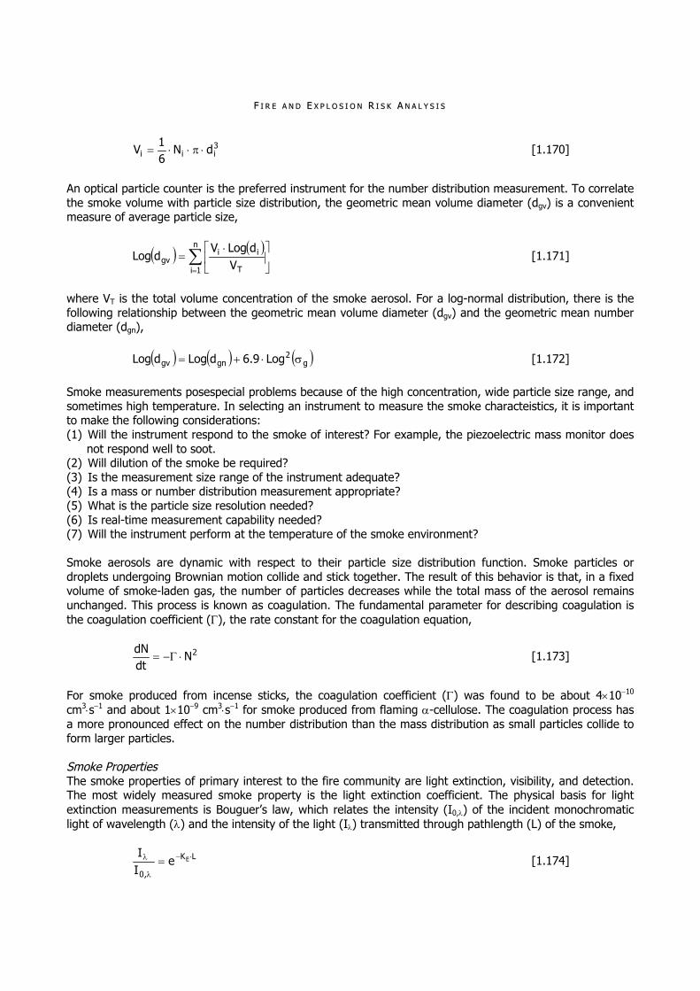
FF II RR EE AA NN DD EE XX PP LL OO SS II OO NN RR II SS KK AA NN AA LL YY SS II SS
3iii dN
61
V [1.170]
An optical particle counter is the preferred instrument for the number distribution measurement. To correlate the smoke volume with particle size distribution, the geometric mean volume diameter (dgv) is a convenient measure of average particle size,
n
1i T
iigv V
dLogVdLog [1.171]
where VT is the total volume concentration of the smoke aerosol. For a log-normal distribution, there is the following relationship between the geometric mean volume diameter (dgv) and the geometric mean number diameter (dgn),
g2
gngv Log9.6dLogdLog [1.172]
Smoke measurements posespecial problems because of the high concentration, wide particle size range, and sometimes high temperature. In selecting an instrument to measure the smoke characteistics, it is important to make the following considerations: (1) Will the instrument respond to the smoke of interest? For example, the piezoelectric mass monitor does
not respond well to soot. (2) Will dilution of the smoke be required? (3) Is the measurement size range of the instrument adequate? (4) Is a mass or number distribution measurement appropriate? (5) What is the particle size resolution needed? (6) Is real-time measurement capability needed? (7) Will the instrument perform at the temperature of the smoke environment? Smoke aerosols are dynamic with respect to their particle size distribution function. Smoke particles or droplets undergoing Brownian motion collide and stick together. The result of this behavior is that, in a fixed volume of smoke-laden gas, the number of particles decreases while the total mass of the aerosol remains unchanged. This process is known as coagulation. The fundamental parameter for describing coagulation is the coagulation coefficient (), the rate constant for the coagulation equation,
2NdtdN
[1.173]
For smoke produced from incense sticks, the coagulation coefficient () was found to be about 41010 cm3s1 and about 1109 cm3s1 for smoke produced from flaming -cellulose. The coagulation process has a more pronounced effect on the number distribution than the mass distribution as small particles collide to form larger particles. Smoke Properties The smoke properties of primary interest to the fire community are light extinction, visibility, and detection. The most widely measured smoke property is the light extinction coefficient. The physical basis for light extinction measurements is Bouguer’s law, which relates the intensity (I0,) of the incident monochromatic light of wavelength () and the intensity of the light (I) transmitted through pathlength (L) of the smoke,
LK
,0
EeII
[1.174]
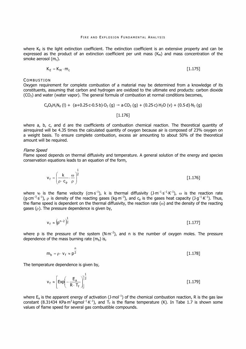
FF II RR EE AA NN DD EE XX PP LL OO SS II OO NN FF UU NN DD AA MM EE NN TT AA LL AA NN AA LL YY SS II SS
where KE is the light extinction coefficient. The extinction coefficient is an extensive property and can be expressed as the product of an extinction coefficient per unit mass (KM) and mass concentration of the smoke aerosol (mc).
cME mKK [1.175] CC OO MM BB UU SS TT II OO NN Oxygen requirement for complete combustion of a material may be determined from a knowledge of its constituents, assuming that carbon and hydrogen are oxidized to the ultimate end products: carbon dioxide (CO2) and water (water vapor). The general formula of combustion at normal conditions becomes,
CaObHcNd (l) + (a+0.25c-0.5b)O2 (g) aCO2 (g) + (0.25c)H2O (v) + (0.5d)N2 (g)
[1.176] where a, b, c, and d are the coefficients of combustion chemical reaction. The theoretical quantity of airrequired will be 4.35 times the calculated quantity of oxygen because air is composed of 23% oxygen on a weight basis. To ensure complete combustion, excess air amounting to about 50% of the theoretical amount will be required. Flame Speed Flame speed depends on thermal diffusivity and temperature. A general solution of the energy and species conservation equations leads to an equation of the form,
21
pf c
kv
[1.176]
where vf is the flame velocity (cms1), k is thermal diffusivity (Jm1s1K1), is the reaction rate (gcm3s1), is density of the reacting gases (kgm3), and cp is the gases heat capacity (Jg1K1). Thus, the flame speed is dependent on the thermal diffusivity, the reaction rate () and the density of the reacting gases (). The pressure dependence is given by,
21
2nf pv [1.177]
where p is the pressure of the system (Nm2), and n is the number of oxygen moles. The pressure dependence of the mass burning rate (mb) is,
2n
fb pvm [1.178] The temperature dependence is given by,
21
f
af TR
EExpv
[1.179]
where Ea is the apparent energy of activation (Jmol1) of the chemical combustion reaction, R is the gas law constant (8.31434 KPam3kgmol1K1), and Tf is the flame temperature (K). In Tabe 1.7 is shown some values of flame speed for several gas combustible compounds.

FF II RR EE AA NN DD EE XX PP LL OO SS II OO NN RR II SS KK AA NN AA LL YY SS II SS
Table 1.7 – Flame speed values for some gas combustible compounds.
OO22 TTff FFllaammee SSppeeeedd GGaass ((mmoolleess)) ((KK)) ((ccmm//ss))
Carbon monoxide 0.5 2977 29 Methane 2.0 3054 43 Ethane 3.5 3086 44 Butane 6.5 3101 45 Propane 5.0 3096 46 Benzene 7.5 3136 48 Acetylene 2.5 3342 144 Hydrogen 0.5 3080 170
Detonation and Deflagration A detonation is a chemically driven shock wave cause by a exothermic material or mixture of materials. Detonation conditions can be calculated from thermodynamics and chemical kinetics. If we assumed the detonation to be «steady state» then no kinetics is considered. Detonation temperatures are similar to combustion temperatues (typical values are approximately 2,500K in air or greater than 3,000K in pure oxygen). We ca find typical detonation velocities of 105 ms1, and detonation pressures are approximately between in the range of 20 to 40 atm. In Table 1.8 is shown the differences between detonation and deflagration processes. Pressure and velocity of detonation are dependent on final products characteristics: molecular weight and reaction temperature. Detonation velocity (vd) is given by the following expression,
ffi
fd TRnv
[1.180]
where f is end products density, i is initial reagents density, nf is the number of moles of the end products, R is the gas law constant measured at end products environmental conditions, and Tf is the end products temperature (K). Detonation velocity is primarily a function of product conditions: (1) Condensed (or high) explosive substances generate very high pressures (approximately greatr than 7
atm). (2) Extremely high pressures generate extremely destructive shock waves. (3) Detonation velocities are approximately 8,000 ms1 to 9,000 ms1.
Table 1.8 – Differences in gaseous detonations and deflagrations.
TTyyppiiccaall RRaattiioo MMaaggnniittuuddee DDeettoonnaattiioonn DDeeffllaaggrraattiioonn
Burned gas velocity / Speed of sound 5 – 10 0.0001 – 0.03 Burned gas velocity / Initial gas velocity 0.4 – 0.7 4 – 16 Final pressure / Initial pressure 13 – 15 0.98 – 0.976 Final temperature / Initial temperature 8 – 21 4 – 16 Final density / Initial density 1.4 – 2.6 0.06 – 0.25
Free Radical Mechanism Hot surface oxidations are commonly thought to involve initial free radical hydrogen atom abstraction. Evidence implicates initial Lewis base deprotonation by atomic oxygen radical anions (O) to form negatively charged carbanions. Subsequent rate determining electron transfers generate free radicals which only then give rise to combustion. Correlations regarding ignition temperatures and hydrocarbon oxidation product identity are consistent with carbanionic but not free radical effects. Highly polarized surfaces (e.g., quartz and corroded surfaces), and addition of polar compounds to fuel and air mixtures facilitate ignitions. EFM confirms increased electrostatic intensities at microscopic surface defects. «Red spot» zones (flameless high temperature zones) are due to flameless oxidations induced by concentrated electrostatic negative charges
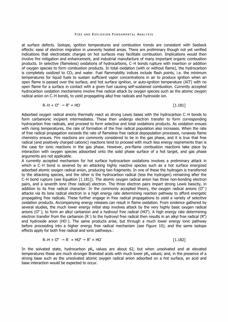
FF II RR EE AA NN DD EE XX PP LL OO SS II OO NN FF UU NN DD AA MM EE NN TT AA LL AA NN AA LL YY SS II SS
at surface defects. Isotope, ignition temperatures and combustion trends are consistent with Seebeck effects: ease of electron migration in unevenly heated areas. There are preliminary though not yet verified indications that electrostatic charges on hot surfaces may facilitate combustion. Implications would then involve fire mitigation and enhancement, and industrial manufacture of many important organic combustion products. In selective (flameless) oxidations of hydrocarbons, CH bonds rupture with insertion or addition of oxygen species to form combustion products. In total oxidation (with or without flame), the hydrocarbon is completely oxidized to CO2 and water. Fuel flammability indices include flash points, i.e. the minimum temperatures for liquid fuels to sustain sufficient vapor concentrations in air to produce ignition when an open flame is passed over the surface, and hot surface ignition, or auto-ignition temperature (AIT) with no open flame for a surface in contact with a given fuel causing self-sustained combustion. Currently accepted hydrocarbon oxidation mechanisms involve free radical attack by oxygen species such as the atomic oxygen radical anion on CH bonds, to yield propagating alkyl free radicals and hydroxide ion.
RH + O R + HO [1.181] Adsorbed oxygen radical anions thermally react as strong Lewis bases with the hydrocarbon CH bonds to form carbanionic incipient intermediates. These then undergo electron transfer to form corresponding hydrocarbon free radicals, and proceed to form selective and total oxidations products. As oxidation ensues with rising temperatures, the rate of formation of the free radical population also increases. When the rate of free radical propagation exceeds the rate of flameless free radical depopulation processes, runaway flame chemistry ensues. Fire reactions are commonly considered to be in the gas phase, and it is true that free radical (and positively charged cationic) reactions tend to proceed with much less energy reqirements than is the case for ionic reactions in the gas phase. However, pre-flame combustion reactions take place by interaction with oxygen species adssorbed onto the solid phase surface of a hot target, and gas phase arguments are not applicable. A currently accepted mechanism for hot surface hydrocarbon oxidations involves a preliminary attack in which a CH bond is severed by an attacking highly reactive species such as a hot surface energized adsorbed atomic oxygen radical anion, producing two fragments. In one of these the hydrogen is transferred to the attacking species, and the other is the hydrocarbon radical (less the hydrogen) remaining after the CH bond rupture (see Equation [1.181]). The atomic oxygen radical anion has three non-bonding electron pairs, and a seventh lone (free radical) electron. The three electron pairs impart strong Lewis basicity, in addition to its free radical character. In the commonly accepted theory, the oxygen radical anions (O) attacks via its lone radical electron in a high energy rate determining reaction pathway to afford energetic propagating free radicals. These further engage in free radical propagations to yield a variety of selective oxidation products. Accompanying energy releases can result in flame oxidation. From evidence gathered by several studies, the much lower energy initial step involves attack by the very highly basic oxygen radical anions (O), to form an alkyl carbanion and a hydroxyl free radical (HO). A high energy rate determining electron transfer from the carbanion (R) to the hydroxyl free radical then results in an alkyl free radical (R) and hydroxide anion (HO). The same products arise, but through a much lower energy ionic pathway before proceeding into a higher energy free radical mechanism (see Figure 10); and the same isotope effects apply for both free radical and ionic pathways.:
RH + O R + HO R + HO [1.182] In the solvated state, hydrocarbon pKa values are about 62, but when unsolvated and at elevated temperatures these are much stronger Brønsted acids with much lower pKa values; and, in the presence of a strong base such as the unsolvated atomic oxygen radical anion adsorbed on a hot surface, an acid and base interaction would be expected to occur.

FF II RR EE AA NN DD EE XX PP LL OO SS II OO NN RR II SS KK AA NN AA LL YY SS II SS
BB II BB LL II OO GG RR AA PP HH YY Faires, Virgel Moring and Simmang, Clifford Max, Thermodynamics, MacMillan Publishing Co. Inc., New York. Finnerty, A. E., 1976. The physical and chemical mechanisms behind fire-safe fuels. BRL-1947, Ballistic Res. Labs, Abderdeen Proving Ground, MD. Hamilton, D. C. and Morgan, N. R., Radiant-interchange configuration factors, Tech. Note 2836, National Advisory Committee for Aeronautics. Holman, J. P., Heat transfer, 3rd Edition, McGraw-Hill, New York. Knudsen, J. G. and Katz, D. L., Fluid dynamics and heat transfer, McGraw-Hill, New York. Kreith, Frank, Principles of heat transfer, 3rd Edition, Intext Press, Inc., New York, ISBN 0-7002-2422-X. McCracken, D. J., 1970. Hydrocarbon combustion and physical properties, Ballistic Research Laboratory Report No. 1496, Aberdeen Proving Ground, Aberdeen, MD. NFPA 325, 1994. Fire hazard properties, flammable liquids, gases and volatile solids. National Fire Protection Association, Boston, pp. 4-5. Pfefferle, L. D., Griffin,T. A., Winter, M., Crosley, D., Dyer, M. J., 1989. Combustion and flame 76, 325-8. R. H. Perry, and C. H. Chilton, Chemical Engineer’s Handbook, 5th ed., New York, McGraw-Hill Book Company, 1973. Reynolds, W. C. and Perkins, H. C., Engineering thermodynamics, 2nd Edition, McGraw-Hill, New York, ISBN 0-07-052046-1. Sparrow, E. M. and Cess, R. E., Radiation heat transfer, Brooks and Cole Publish. Co., Belmont, California. VanWylen, G. J. and Sonntag, R. E., Fundamentals of classical thermodynamics, 2nd Edition, John Wiley and Sons, New York, ISBN 0-471-04188-2. Weibelt, J. A., Engineering radiation heat transfer, Holt, Rinehart and Winston Publish., New York.
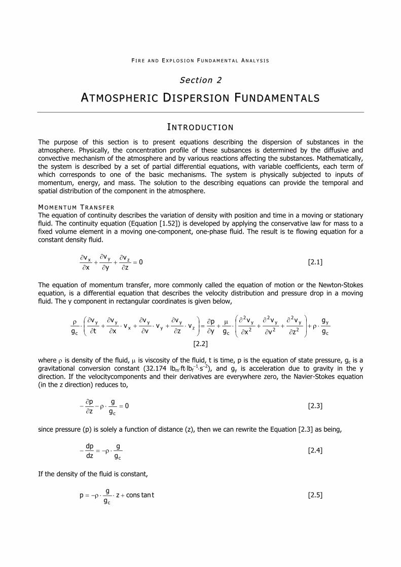
FF II RR EE AA NN DD EE XX PP LL OO SS II OO NN FF UU NN DD AA MM EE NN TT AA LL AA NN AA LL YY SS II SS
SS ee cc tt ii oo nn 22
AATTMMOOSSPPHHEERRIICC DD II SSPPEERRSS IIOONN FFUUNNDDAAMMEENNTTAALLSS
II NN TT RR OO DD UU CC TT II OO NN The purpose of this section is to present equations describing the dispersion of substances in the atmosphere. Physically, the concentration profile of these subsances is determined by the diffusive and convective mechanism of the atmosphere and by various reactions affecting the substances. Mathematically, the system is described by a set of partial differential equations, with variable coefficients, each term of which corresponds to one of the basic mechanisms. The system is physically subjected to inputs of momentum, energy, and mass. The solution to the describing equations can provide the temporal and spatial distribution of the component in the atmosphere. MM OO MM EE NN TT UU MM TT RR AA NN SS FF EE RR The equation of continuity describes the variation of density with position and time in a moving or stationary fluid. The continuity equation (Equation [1.52]) is developed by applying the conservative law for mass to a fixed volume element in a moving one-component, one-phase fluid. The result is te flowing equation for a constant density fluid.
0z
vy
v
xv zyx
[2.1]
The equation of momentum transfer, more commonly called the equation of motion or the Newton-Stokes equation, is a differential equation that describes the velocity distribution and pressure drop in a moving fluid. The y component in rectangular coordinates is given below,
c
y2y
2
2y
2
2y
2
cz
yy
yx
yy
c g
g
z
v
v
v
x
v
gyp
vz
vv
v
vv
x
v
t
v
g
[2.2] where is density of the fluid, is viscosity of the fluid, t is time, p is the equation of state pressure, gc is a gravitational conversion constant (32.174 lbmftlbf
1s2), and gy is acceleration due to gravity in the y direction. If the velocitycomponents and their derivatives are everywhere zero, the Navier-Stokes equation (in the z direction) reduces to,
0gg
zp
c
[2.3]
since pressure (p) is solely a function of distance (z), then we can rewrite the Equation [2.3] as being,
cgg
dzdp
[2.4]
If the density of the fluid is constant,
ttanconszgg
pc
[2.5]

FF II RR EE AA NN DD EE XX PP LL OO SS II OO NN RR II SS KK AA NN AA LL YY SS II SS
This is the equation describing the hydrostatic pressure in a system. If pressure (p) is ph when z is h, the Equation [2.5] becomes,
zhgg
ppc
h [2.6]
Equation [2.3] may be used to describe pressure variations in the atmosphere. Where the fluid may no longer be assumed incompressible, the decrease in the gravity force also produces a decrease in pressure. The emperature is, of course, then dictated by the equation of state of the air. If ideal gas conditions are assumed, the equation of state is given by,
TRp
y
[2.7]
so that
TRp
gg
dzdp
c [2.8]
If the temperature of the air is constant (isothermal), the integrated form of Equation [2.8] becomes,
dzTR
1gg
pdp
c
[2.9]
Simplifying Equation [2.9] and solving to pressure (p) and distance (z) becomes,
TRhz
gg
hcepp [2.10]
The variation of density with height under isothermal conditions is given by a similar expression.
TRhz
gg
hce [2.11]
If the air system is assumed adiabatic, one can show that,
1
hh pp
TT
[2.12]
or the equivalent expression,
TdT
1pdp
[2.13]
where
v
p
c
c [2.14]
Substituting Equation [2.13] into Equation [2.8] gives,

FF II RR EE AA NN DD EE XX PP LL OO SS II OO NN FF UU NN DD AA MM EE NN TT AA LL AA NN AA LL YY SS II SS
1Rg
gdzdT
c [2.15]
Employing values for air, it yields,
1ftFº00535.0dzdT [2.16]
1mCº01.0
dzdT [2.17]
The wind profle can reasonably be approximated by the simple power law relationship normally applicable for turbulent flow systems,
q
h,yy hz
vv
[2.18]
with vy,h as the velocity of y component at a given distance (h), and constant q > 0. A corresponding expression for the eddy viscosity is,
q1
h hz
[2.19]
An equivalent form of Equation [2.18] for the velocity gradient is given by,
zdz
dv y [2.20]
where is a constant and independen of z, and is a strong function of meteoroligical conditions. EE NN EE RR GG YY TT RR AA NN SS FF EE RR The general conservation law for enegy on a rate basis is applied to obtain the equation of energy transfer. In most engineering applications, the following assumptions are introduced in order to simplify the describing equations: (1) Viscous effects are negligible; (2) Kinetic and potential energy changes are small; (3) The fluid is incompressible; (4) The heat capacity is constant. The equation of heat transfer is presented below in rectangular coordinates,
p2
2
2
2
2
2
Pzyx c
Q
z
T
v
T
x
Tc
kzT
vyT
vxT
vtT
[2.21]
where k is the thermal conductivity, cp is the heat capacity, Q is the rate of energy generated per unit volume.

FF II RR EE AA NN DD EE XX PP LL OO SS II OO NN RR II SS KK AA NN AA LL YY SS II SS
AA TT MM OO SS PP HH EE RR II CC MM AA SS SS TT RR AA NN SS FF EE RR The equation describing mass transfer within a system containing a one (pure) component fluid without chemical reaction was given in Equation [2.2] of momentum transfer. This is defined as he equation of continuity. The equation for mass transfer differs from the equation of continuity in that it contains terms accounting for molecular diffusion and chemical reaction effects. The phenomenological law governing the transfer of mass by molecular diffusion is the Fick’s law. Mass transfer processes usually involve the transfer of more than one component. A more than one component system is defined as binary (two component) or multicomponent (three or more components). For a multicomponent mixture, vi is denoted as the velocity of the i-th component relative to a fixed origin coodinated system. The mxture’s average velocity on a mass basis is defined as being,
j
1iiij
1ii
j
1iii
avg vwv
v [2.22]
where i is the mass concentration (kgm3) of component, wi is mass fraction of component, and j is the number of components in mixture. It is the velocity employed in the continuity equation and equation of motion. The following enumerates the rate of mass (in units of moles) conserved within the moving fluid contained in the volume element (V) at any time. [rate of moles input by molecular diffusion][rate of moles output by molecular diffusion]+[rate of moles
input by convection][ rate of moles output by convection]+[rate of moles generated]=[rate of moles
accumulated]
[2.23] The equation which results is presented as given,
iz,iy,ix,ii
zi
yi
xi R
z
J
y
J
x
J
zC
vyC
vxC
vtC
[2.24]
where Ci is instantaneous concentration; vx, vy, and vz are the velocity components in x, y, and z directions; Ri is the moles generated; and Ji is the molar flux of i component.
xC
DJ ix,i
[2.25]
yC
DJ iy,i
[2.26]
zC
DJ iz,i
[2.27]
where D is the diffusion coefficient (m2s1). Substituting Equation [2.25] through Equation [2.27] on Equation [2.24], then we have the following expression,
i2i
2
2i
2
2i
2i
zi
yi
x Rz
C
y
C
x
CD
zC
vyC
vxC
v
[2.28]

FF II RR EE AA NN DD EE XX PP LL OO SS II OO NN FF UU NN DD AA MM EE NN TT AA LL AA NN AA LL YY SS II SS
Due to turbulence, the turbulent diffusion coefficient for the system may not be isotropic, i.e. independent of direction. If this coefficientis a function of direction, the effect is said to be anisotropic. Under these conditions, the Equation [2.28] becomes,
i2i
2
z2i
2
y2i
2
xi
zi
yi
xi R
z
CD
y
CD
x
CD
zC
vyC
vxC
vtC
[2.29]
where Dx, Dy, and Dz are the diffusion coefficients in the x, y, and z directions, respectively, and have been assumed independent of position. If exists, chemical reaction effects in the atmosphere are often represented by first order kinetics in the source term (Ri) in the describing equation, i.e. the rate of reaction is proportional to the concentration of the substane in question. The vertical diffusion coefficient (Dz) is generally assign a simple power law relation similar to,
q1
h,zz hz
DD
[2.30]
and q 0. horizontal diffusion in the direction of bulk flow is neglected since the convective effects far outweigh diffusion. The variation of wind profile in the vertical direction is usually given by another power law expression,
q
h,yy hz
vv
[2.31]
although q is often assumed to be 71
, q is an index of atmospheric stability. For unstable conditions q
approachs to zero, while for stable and inversion condtions q is greater than 71
. In order to provide a better
understanding and appreciation of the describing equation for atmospheric dispersion system, considering the case of any air component, initially present at uniform concentration (C0,i), or not present, at initial time equal to zero (t = 0), the diffusion process is assuming to be commenced it is proposed to calculate the concentration of component i as a function of position (y) and time (t) and to be obtain the mass flux at the initial interface. The initial concentration profile is given by the following expression,
t,yCC ii [2.32] and vx = vy = vz = 0. the partial differential equation describing this system is,
2i
2
yi
y
CD
tC
[2.33]
Begin by multiplying both sides of Equation [2.33] by,
dte tp [2.34] and integrating from 0 to becomes,
02
i2
tpy
0
itp dty
CeDdt
tC
e [2.35]

FF II RR EE AA NN DD EE XX PP LL OO SS II OO NN RR II SS KK AA NN AA LL YY SS II SS
The integration by parts of Equation [2.35] gives the following expression,
tD4
y
iy
2
et
1t,yC [2.36]
Note that the flux is a function of time and decreases with time. The total quantity of mass (ni) per unit area (A) transferred with time is given by,
tD
CAn
i,0i [2.37]
Incorporating chemical kinetics, the partial differential equation describing the system becomes,
i2i
2
yi Ck
y
CD
tC
[2.38]
here k is the reaction constant. The integration of Equation [2.38] becomes,
dy'yCet
1et,yC i
tD4y
tki
y
2
[2.39]
If the location of the source is changed from point zero (0) to point y = y’ the particle y2 becomes (yy’)2. the partial differential equation describing the chemical reaction and convection combined system becomes,
i2i
2
yyii Ck
y
CDv
yC
tC
[2.40]
The equation describing the concentration due to an instantaneous source of mass of component i at initial time (t = 0) and y = 0 is given by,
tD4
y
y
ii
y
2
etD4A
dnt,ydC [2.41]
If no diffusion occurred, the differential equation is given by the following expression,
ii Ck
dtdC
[2.42]
with solution
tki,0i eCC [2.43]
where C0,i is the initial concentration of component i at any position y in the system. The solution to Equation [2.40] is the followig,
FF II RR EE AA NN DD EE XX PP LL OO SS II OO NN FF UU NN DD AA MM EE NN TT AA LL AA NN AA LL YY SS II SS
'dy'yCetD4
1et,yC i
tD4
tv'ytvy
y
tki
y
yy
[2.44]
where Ci(y’) is the initial concentration profile. The describing partial differential equation for a two-dimensional system is,
2i
2
2i
2i
z
C
y
CD
tC
[2.45]
The verified solution to this equation is given by,
'y
'y
'z
'zi
tD4'zz'yy
i 'dz'dy'z,'yCetD4
1t,yC
22
[2.46]
where Ci(y’,z’) is the initial concentration profile, and Dy = Dz = D. For a three-dimensional system, the describing partial differentia equation is,
2i
2
2i
2
2i
2i
z
C
y
C
x
CD
tC
[2.47]
with the solution
'x
'x
'y
'y
'z
'zi
tD4'zz'yy'xx
23i 'dz'dy'dx'z,'y,'xCe
tD4
1t,yC
222
[2.48]
AA TT MM OO SS PP HH EE RR II CC DD II FF FF UU SS II OO NN CC OO EE FF FF II CC II EE NN TT SS With motion solely in the y direction, x represents the lateral or cosswind coordinate, y is the downwind coordinate, and z is the vertical coordinate. A front and top concentration profile of a three-dimensional plume is given in Figure 2.1. The essential feature of the dispersion of the component is that the concentration profile has a Gaussian or normal distribution with standard deviations x and z in the x and z directions. The diffusive effect in the direction of motion (y) is neglected. The standard deviations can than be related to the turbulent diffusion coefficient by the equation,
tD22 [2.49] which is identical in form to the equation proposed by Einstein for brownian (random or chaotic as in turbulent flow) motion. If the above equation is referred to an coordinate system fixed in space, then we can have the following expression,
vSD22
[2.50]
where S is displacement (m) of the fluid in the direction of bulk flow relative to the origin in time (t), v is bulk (mean) windspeed (ms1) of the fluid, and D is diffusion coefficient in a plane perpendicular to the direction of bulk motion. Thus,

FF II RR EE AA NN DD EE XX PP LL OO SS II OO NN RR II SS KK AA NN AA LL YY SS II SS
yx
x2x vv
yD2
[2.51]
yz
z2z vv
yD2
[2.52]
If we consider the diffusion effect in the y direction of motion, the standard deviation is,
2y
y2y
v
yD2 [2.53]
z
x
vy
y
Front View
z
yz z z
Top View
x
yx x x
Figure 1.1 – Schematic three-dimensional concentration profile for air system components behavior. In addiion to varying with downwind direction (y), x and z are strong functions of turbulence in the atmosphere, meteorological conditions, and topography. The literature suggests equations for standard deviations (x and z) of the form,
axx yb [2.54]
a
zz yb [2.55]

FF II RR EE AA NN DD EE XX PP LL OO SS II OO NN FF UU NN DD AA MM EE NN TT AA LL AA NN AA LL YY SS II SS
where the coefficients a, bx, and bz are empiracally determined constant that depend on the state (stability) of the atmosphere. In addition, the systemis often assumed isotropic so that,
zx [2.56] The usual procedure in applied meteorology is to write the solutions to the describing equations in terms of standard deviations. For example, the equation for instantaneous point discharge at time equal to zero is,
2r21
23
2
ii e
2
nC
[2.57]
where ni is the moles discharged, and is he standard deviation calculated by Equation [2.49]. For an anisotropic medium it becomes,
2
z
2
y
2
x
zyx21
zyx3
ii e
8
nC [2.58]
with the source located at the origin. For the continuous source, located in a medium moving with velocity vy, with respect to time from zero to (infinite) gives,
2
z
2
x
zx21
zyx
ii e
2n
C [2.59]
where the diffusive effect in the direction of motion has been neglected. Since most continuous sources are located at or near the earth’s surface, it is necessary to account for this effect. The result is the following,
2
z
2
z
2
x
hz21
exphz
21
expx
21
zyx
ii e
2n
C [2.60]
where z is the levation of the source above the ground plane. If the receptor is locared at the ground level (z = 0) we have the foowing mathematical relation,
2
z
2
x
hx21
zyx
ii e
2n
C [2.61]
which is the form of equation most often used in atmospheric dispersion prediction techniques. TT OO PP OO GG RR AA PP HH YY AA NN DD MM EE TT EE OO RR OO LL OO GG II CC AA LL CC OO NN DD II TT II OO NN SS The definition of air components is a direct result of atmospheric turbulence and a molecular diffusion. Atmospheric turbulence and, hence, atmosperic diffusion vary widely with weather conditions and topography. Unfavorable meteorological condition is the presence of an inversion layer over the region of the plume dispersion. Stable thermal conditions in an inversion suppress vertical atmospheric turbulence and the dispersal of gases. With an inversion layer above a more turbulent region, gases disperse downward, thus causing greater groundlevel concentrations. This situation becomes particularly acute in a region of unfavorable topographical features, such as in a valley when the valley walls prevent lateral air motion and inversion layer act as a lid over the valley depression. Unfavorable local configuration and topography
FF II RR EE AA NN DD EE XX PP LL OO SS II OO NN RR II SS KK AA NN AA LL YY SS II SS
produce turbulence and distortion of air motion, which cause gases and vapors to disperse downward toward the ground more rapidly then upward. These will occur when fire stack heig and characteristics of gases (and fumes) are not sufficient to carry the plume above the layer of strong turbulence. TT UU RR BB UU LL EE NN TT EE DD DD YY DD II FF FF UU SS II OO NN The momentum of the wind near the earth is continually dissipated by the friction at the earth’s surface. The mechanism which brings about this interchange of mass is known as turbulent eddy diffusion. Mechanical turbulence is inuced by the movement of wind over the aerodynamic rough surface of the earth and is proportional to the surface roughness and wind speed. Thermal turbulence is solar-induced and is a function of latitude, the radiating surface, and the stability of the environment. Near the ground, turbulence or eddy motion is also set up by obstacles introduced into the direct flow of air by the surface and its irregularities. Verticals transports of momentum, heat, and waer vapor in the atmosphere are all function of turbulence, which have a random nature. PP OO TT EE NN CC II AA LL TT EE MM PP EE RR AA TT UU RR EE AA NN DD AA TT MM OO SS PP HH EE RR II CC SS TT AA BB II LL II TT YY The earth’s atmosphere is nory treated as a perfect gas mixture. The volume of such an air parcel must be inversely prportional to the density. The perfect gas law,
TRVP [2.62] becomes
TRP [2.63] Therefore, heat transfer in the atmosphere is caused by radiative heating or by mixing due to turbulence (convective transfer). If there is no mixing, an air parcel rises adiabatically (no heat transfer) in the atmosphere. The air pressure at a fixed point is caused by weight of the air above that point. The change in pressure is proportional to the change in height,
dzgdP [2.64] This is a hydrostatic pressure distribution. Since the air is compressible, the density is also a decreasing function of height. As the pressure drops, the parcel must expand adiabatically. The work done in the adiabatic expansion (PdV) comes from the thermal energy of the air parcel. As the parcel expands, the internal energy decreases and the temperature also decreases. The rate of expansion with altitude is fixed by the vertical pressure variation establish by Equation [2.64]. The vertical temperature gradient in the atmosphere is called the lapse rate. The dry adiabatic lapse rate (DALR) will be approximated as,
1ftFº00535.0dzdT [2.16]
or
1mCº01.0dzdT [2.17]
If the rising air contains water vapor, the cooling due to adiabatic expansion will result in the relative humidity being increased and saturation may be reahed. Further ascend would then lead to condensation of water vapor, and the latent heat thus released would reduce the rte of cooling of the rising air. The buoyancy force on a warm air parcel is caused by the difference between its density and that of the surrounding air. The temperature is normally used because it is easier to measure than the density. Once a parcel of air is started moving up or down, it will continue to do so, causing unstable atmospheric conditions. If the temperature decreases more slowly with increasing altitude than the adiabatic lapse rate, a dispaced parcel of air experiences a net restoring force. The buoyancy forces cause stable atmospheric conditions.

FF II RR EE AA NN DD EE XX PP LL OO SS II OO NN FF UU NN DD AA MM EE NN TT AA LL AA NN AA LL YY SS II SS
Stable conditions: 1mCº01.0dzdT [2.65]
Neutral conditions: 1mCº01.0dzdT [2.66]
Unstable conditions: 1mCº01.0dzdT [2.67]
The potential temperature (T) is often more convenient to use than the measured than the measured temperature (T). The potential temperature is the temperature a parcel of air would have if it were compressed adiabatically to some reference pressure (approximately 1,000 mbar at ground level). The relation between the potential temperature and the measured temperature is,
z108.9TT 3 [2.68]
where z is the height (m) above the ground (reference pressure) and T is the absolute temperature (K). an isothermal temperature gradient,
0dzdT
[2.69]
and
1mCº01.0dz
dT [2.70]
represents a faily strongly stratified, stable condition. Large-scale unstable lapse rates seldom occur.
1mCº01.0dzdT [2.67]
and
0dz
dT [2.72]
If a such condition were occur, the buoyancy forces would cause the air to redistribute itself to form neutral conditions. The only time unstable conditions are observed for extended periods of time is during strong solar heating. Strongly stable lapse rates are commonly referrred to as inversion.
0dzdT
[2.73]
and
1mCº01.0dz
dT [2.74]
The strong stability inhibits mixing across the inversion layer. Normally these conditions of strong stability only extend for several hundred meters vertically, usually referred as the inversion depth. Ground-level

FF II RR EE AA NN DD EE XX PP LL OO SS II OO NN RR II SS KK AA NN AA LL YY SS II SS
inversions inhibit the downward mixing of components emitted from smoke. This decreases the ground-level concentrations of these components. With the advent of daylight, the ground begins to heat and the inversion is gradually destroyed. EE FF FF EE CC TT II VV EE HH EE II GG HH TT OO FF AA NN EE MM II SS SS II OO NN The effective height of an emission rarely corresponds to the physical height of fire. If the plume is caught in the turulent wake of the fire or in the vicinity, the effluent will be mixed rapidly downward toward the ground. If th plume is emitted free of these turbulent zones, a number of emission factor and meteorological factors influence the rise of the plume. The emission factors include the gas flow (smoke and other components) rate and temperature of the effluent, and the diameter of the fire basis. The meteorological factors influencing plume rise and wind speed are air temperature, shear of the wind speed with height, and atmosphere stability. Plume height is a function of rise due to both momentum and buoyancy. So, plume rise (hv,max) due to momentum is given by the following expression,
v
vG
vv
43.01
77.4h s
s
max,v
[2.75]
where hv,max is maximum momentum rise of plume (ft), v is the wind velocity (fts1), vs is velocity at the exit in fire stack (fts1), and G is gas flow rate from fire stack (ft3s1). The momentum rise of plume at a distance downwind (x) from fire stack is given by,
x
h8.01hh max,v
max,vx,v [2.76]
where distance downwind (x) must be greater than 2hv,max. The plume rise due to buoyancy is,
2
j2
jLnTv
TTGg37.6h 2
3G
T [2.77]
where hT is the maximum thermalrise of plume (ft), g is gravity acceleration constant (32.174 fts1), TF is absolute temperature (K) of gas (smoke) at the interface with fire stack, and T is the absolute temperature (K) at which density of gases equals the density of the ambient atmosphere.
1TT
Tgv
28.0Tg
T43.0
vG
vj
F
s
s
2
[2.78]
The Equation [2.77] is valid when the following condition applies,
5.0
sF
2
vG
TTT
gv
[2.79]
Otherwise hT is eiminated from the summation for the effective height (hef) of emission,
Tmax,vsef hhhh [2.80]
where hs is the physical fire stack height (ft), and T is the gradient of potencial atmospheric temperature,
dzdT
T [2.81]

FF II RR EE AA NN DD EE XX PP LL OO SS II OO NN FF UU NN DD AA MM EE NN TT AA LL AA NN AA LL YY SS II SS
For an adiabatic lapse rate, T = 0ºCft1; for an isothermal lapse rate, T = 0.003ºCft1; and for a strong inversion, T = 0.006ºCft1. It is suggested a value of a gradient of potencial atmospheric temperature (T) for normal atmospheric conditions as 0.001ºCft1. From Figure 1.1, we can obseerve that the plume travels along or parallel to the y axis (in the mean wind direction). The concentration (Ci, gm3) of gas (smoke) or aerosols at point (x,y,z) from a continuous source with an effective emission height (hef), in metric units, is given by the following expression,
2
z
ef2
z
ef2
x
hz21
exphz
21
expx
21
zxefi e
v2G
h,z,y,xC [2.82]
where v is mean wind speed affecting the plume (ms1), G is emission rate of gas or components (gs1), x and y are stability parameters in x and z directions (m). It is necessary to estimate concentrations from a single source for the time intervals greater than few minutes; the best estimate is obtained from,
p
s
kk,is,i t
tCC
[2.83]
where Ci,s is the desired concentration estimate for sampling time (ts), and Ci,k is the concentration for the shorter sampling time (tk), and p is a constant between 0.17 and 0.20; the latter value is more commonly used. SS MM OO KK EE TT RR AA NN SS FF EE RR FF II LL MM TT HH EE OO RR YY Smoke transfer may be defined as the process by which smoke is transferred from one point to another. Over the past 55 years, a number of mass transfer theories have been proposed to explain the mechanism of smoke transfer. The simplest and the one most commonly used is the two-film theory proposed by Lewis and Whitman in 1924. The two-film theory remains popular because, in more than 95% of the situations encountered, the results obtained are essentially the same as those obtained with the more complex theories. The two-film theory is based on a physical model in which two-films exist at the interface (i.e. gas-to-gas interface, or in other cases, gas-to-liquid interface and liquid-to-liquid interface). In the systems use, the rate of smoke transfer is generally proportional to the difference between the existing concentration an the equilibrium concentration of the smoke. An equation from this relationship can be expressed as,
CCAkr sgg [2.84]
where rg is the rate of mass transfer, kg is the coefficient of diffusion, Cs is the saturation concentration of smoke, and C is the ominal concentration. Under the conditions of mass transfer encountered,
dtdC
Vrg [2.85]
and substituting Equation [2.85] in Equation [2.84] it becomes,
CCVA
kdtdC
r sgg
[2.86]
In practice, the term
VA
k g is replaced by a proportionality factor that is related to existing conditions of
exposure. This factor is identified in literature as the overall mass transfer coefficient (km) in units s1. The integrated form of Equation [2.86] is obtained by the following expression,

FF II RR EE AA NN DD EE XX PP LL OO SS II OO NN RR II SS KK AA NN AA LL YY SS II SS
t
0
C
0Cg
sdt
VA
kCC
dC [2.87]
which when solved yields,
tmk
0s
ts eCCCC
[2.88]
with the mass transfer coefficient being given by,
VA
kk gm [2.89]
In Equation [2.90], the terms CsCt and CsC0 represent the final and initial smoke saturation deficits.
BB II BB LL II OO GG RR AA PP HH YY Bird, R. B., Stewart, W., Lightfoot, E., Transport phenomena, John Wiley and Sons, New York, 1960. Pasquill, F., Atmospheric diffusion, Van Nostrand, Princeton, N. J., 1962. Slattry, J., Momentum, energy, and mass transfer in continua, McGraw-Hill, New York, 1972.

FF II RR EE AA NN DD EE XX PP LL OO SS II OO NN FF UU NN DD AA MM EE NN TT AA LL AA NN AA LL YY SS II SS
SS ee cc tt ii oo nn 33
FF IIRREE AANNDD EEXXPPLLOOSS IIOONN RR II SSKK
II NN TT RR OO DD UU CC TT II OO NN Accidents such as at Bhopal (India) in 1984, where methyl isocyanine escaped from a storage facility causing many deaths, have left the impression on the general public that storage of hazardous and toxic materials is extremely dangerous to the public. In Malaysia, the fire and explosion incident at the Bright Sparklers Factory at Baru Sungai Buloh on May 1991 had revealed many shortcomings and the lack of understanding in handling the flammable and explosive materials. Flammable and explosive materials should be handled and stored in the proper manner to avoid any adverse event occur. Fire and explosion are the two major incidents, which could occur in mishandling and storage of flammable and explosive materials. Improper handling found as the major causes in contributing the fire and explosion to occur. Due of that issue, the need for risk assessment and analysis study for handling and storage flammable and explosive materials has become exceedingly critical due to the increasing on the number of accidents. Moreover the potential damage has been magnified by the proximity of many such operations have densely populated areas. The need for risk assessment study concerning the application of hazardous and toxic materials has becomes more important in recent years. It has been found that in many cases risk assessment study of handling hazardous and toxic materials will show the storage area has the greater potential for risk to the public. This is because of the much larger amount of hazardous material usually found in storage compared with process areas, although process areas have accidents more often than storage areas. There is always an element of risk associated with the use, storage and the handling of flammable and explosive materials. Risk from fire and explosive events could be reducing if good design practices are incorporated into process, facilities and building storage. The degree of risk of the fire and explosion hazards is best compared to commonly accepted risk level. Thus, the Asian Development Bank in its Environment Risk Assessment guidelines (Carpenter et al., 1990) suggested that for a project to be acceptable, its potential cumulative risk must not exceed the commonly accepted individual voluntary risk, which is 4 to 10 fatalities per person per year for workers. In addition, if the risk of the operation extends to its neighbouring population, such a risk shall not exceed the commonly acceptable risk level of 6 to 10 fatalities per person per year for surrounding residents. The average individual voluntary risk for fatality to the workers at the quarry industry is calculated to be 5.75 x 10⁻⁶ per person per year, which is much lower than the acceptable level. For instance, eardrum rupture (one of the hazards derived from explosion danger) has been calculated to be 3.15 x 10⁻⁶ per person per year. The risk had been estimated in term of fatalities.
UU NN DD EE RR SS TT AA NN DD FF II RR EE HH AA ZZ AA RR DD SS The potential for air and hydrocarbons to mixture is an inherent risk in oil and gas operations. As a result, the industry continues to experience serious oilfield fires and explosions that injure and kill workers. The canadian Industry Recommended Practice (IRP 18) is aimed at prevention of fire and explosion incidents. This is part of an initiative to increase the awareness of the hazards related to fuel and air mixtures, a fundamental step to improving industry safety. Research to assist with the preparation of IRP 18 included the analysis of 40 incidents. Table 3.1 summarizes the main categories of incidents identified in onshore hydrocarbon exploration industry.
Table 3.1 – Incidents assessed during IRP 18 review to onshore hydrocarbon exploration industry.
IInncciiddeennttss %% WWeellll CCoonnssttrruuccttiioonn OOppeerraattiioonnss %% Production operation incidents 27 Snubbing 5 Repair and maintenance incidents 21 Swabbing 3 Trucking operations incidents 21 Well testing and flowing 15 Well construction operations 32 Hydrocarbon pumping 5 Coiled tubing 3
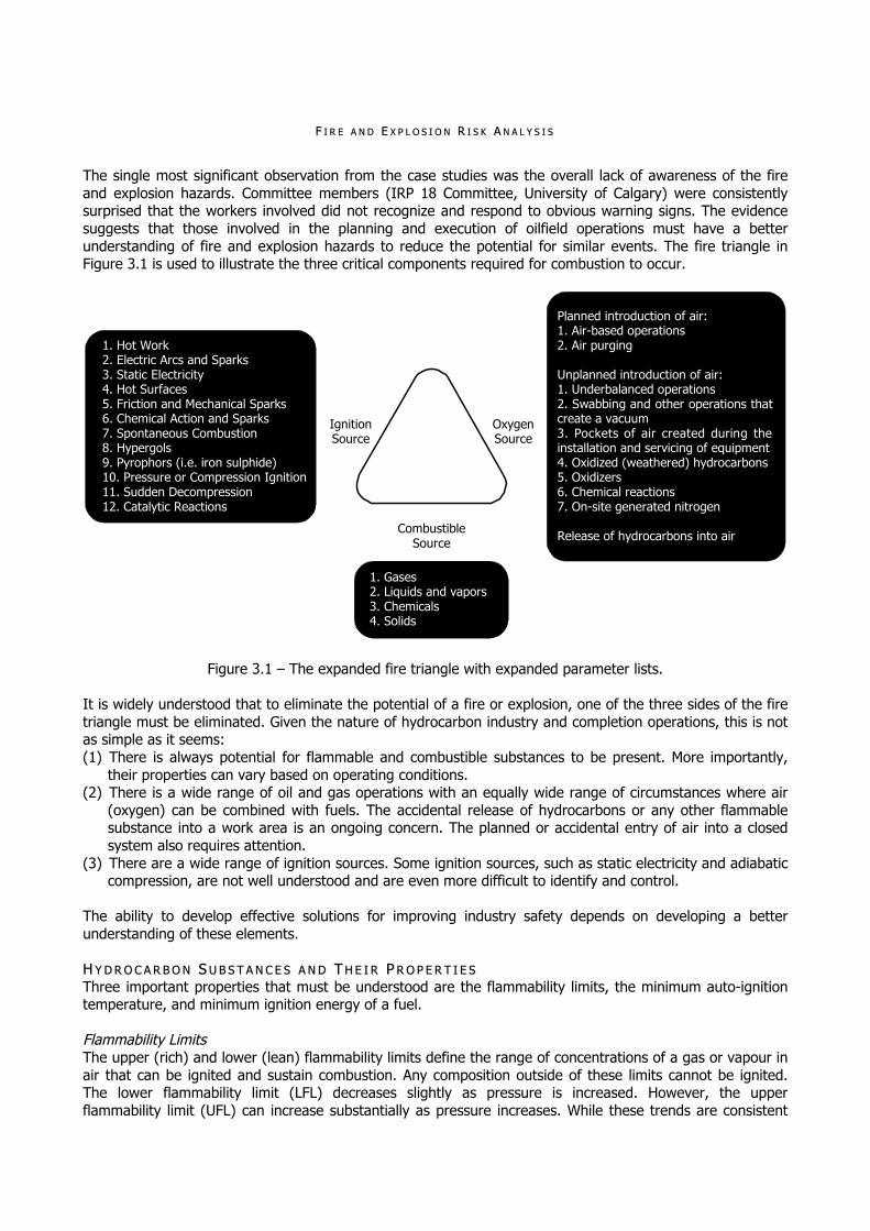
FF II RR EE AA NN DD EE XX PP LL OO SS II OO NN RR II SS KK AA NN AA LL YY SS II SS
The single most significant observation from the case studies was the overall lack of awareness of the fire and explosion hazards. Committee members (IRP 18 Committee, University of Calgary) were consistently surprised that the workers involved did not recognize and respond to obvious warning signs. The evidence suggests that those involved in the planning and execution of oilfield operations must have a better understanding of fire and explosion hazards to reduce the potential for similar events. The fire triangle in Figure 3.1 is used to illustrate the three critical components required for combustion to occur.
1. Hot Work2. Electric Arcs and Sparks3. Static Electricity4. Hot Surfaces5. Friction and Mechanical Sparks6. Chemical Action and Sparks7. Spontaneous Combustion8. Hypergols9. Pyrophors (i.e. iron sulphide)10. Pressure or Compression Ignition11. Sudden Decompression12. Catalytic Reactions
OxygenSource
CombustibleSource
IgnitionSource
Planned introduction of air:1. Air-based operations2. Air purging
Unplanned introduction of air:1. Underbalanced operations2. Swabbing and other operations thatcreate a vacuum3. Pockets of air created during theinstallation and servicing of equipment4. Oxidized (weathered) hydrocarbons5. Oxidizers6. Chemical reactions7. On-site generated nitrogen
Release of hydrocarbons into air
1. Gases2. Liquids and vapors3. Chemicals4. Solids
Figure 3.1 – The expanded fire triangle with expanded parameter lists. It is widely understood that to eliminate the potential of a fire or explosion, one of the three sides of the fire triangle must be eliminated. Given the nature of hydrocarbon industry and completion operations, this is not as simple as it seems: (1) There is always potential for flammable and combustible substances to be present. More importantly,
their properties can vary based on operating conditions. (2) There is a wide range of oil and gas operations with an equally wide range of circumstances where air
(oxygen) can be combined with fuels. The accidental release of hydrocarbons or any other flammable substance into a work area is an ongoing concern. The planned or accidental entry of air into a closed system also requires attention.
(3) There are a wide range of ignition sources. Some ignition sources, such as static electricity and adiabatic compression, are not well understood and are even more difficult to identify and control.
The ability to develop effective solutions for improving industry safety depends on developing a better understanding of these elements. HH YY DD RR OO CC AA RR BB OO NN SS UU BB SS TT AA NN CC EE SS AA NN DD TT HH EE II RR PP RR OO PP EE RR TT II EE SS Three important properties that must be understood are the flammability limits, the minimum auto-ignition temperature, and minimum ignition energy of a fuel. Flammability Limits The upper (rich) and lower (lean) flammability limits define the range of concentrations of a gas or vapour in air that can be ignited and sustain combustion. Any composition outside of these limits cannot be ignited. The lower flammability limit (LFL) decreases slightly as pressure is increased. However, the upper flammability limit (UFL) can increase substantially as pressure increases. While these trends are consistent

FF II RR EE AA NN DD EE XX PP LL OO SS II OO NN FF UU NN DD AA MM EE NN TT AA LL AA NN AA LL YY SS II SS
for all hydrocarbons, each fuel or combustible has a different flammable range. Other factors that widen the flammability range include: (1) Increased temperatures widen the flammable range. (2) Flammability limits are widened by the increased energy of the ignition source. (3) If pure oxygen, instead of air, mixes with a hydrocarbon, the flammability limits may be widened.
Moisture and other contaminants will also affect the flammability range. Auto-ignition Temperature A fuel (or any other combustible) and air mixture can ignite without the introduction of an ignition source. The minimum auto-ignition temperature (AITmin) is the lowest temperature at which the fuel (combustible or flammable material) vapours spontaneously ignite. Hydrocarbons that have been heated can ignite if they are exposed to air. Methane has the highest auto-ignition temperature (540ºC or 1004ºF). As the number of carbon atoms present in the hydrocarbon substance increases, the auto-ignition temperature decreases. In other words, heavier hydrocarbons tend to auto-ignite before lighter hydrocarbons. Increased pressures can also reduce the auto-ignition temperature. Minimum Ignition Energy The minimum amount of energy supplied that is needed for combustion is the minimum ignition energy (IEmin). Every different hydrocarbon and air mixture will have different minimum ignition energies. Factors that affect the minimum ignition energy are: (1) The temperature. (2) The total energy supplied. (3) The rate at which energy is supplied, or time period over which it is delivered. (4) The area over which energy is delivered. The minimum ignition energy values are usually given as the energy required to ignite the most reactive mixture of hydrocarbon and air. A flammable mixture that is close to either the upper or lower limits may require a higher amount of energy than the minimum ignition energy to ignite. Other Relevant Hydrocarbon Considerations With the exception of a few reactive or unstable substances, liquids do not ignite. It is in fact the vapours given off from the surface of the liquids that ignite. Liquids will give off vapours at some temperature. The ability to give off vapours and the rate at which this occurs defines the volatility of the liquid. The flash point (TFP) temperature should only be used as an approximate reference. The liquid may behave differently in the field than in laboratory tests performed to determine flash points. It is possible for an explosive atmosphere to exist even if the temperature of the environment is below the flash point of the liquid. The auto-ignition temperature for the liquid vapours is similar to that of gases. A very fine mist from a hydrocarbon liquid may act as a pure gaseous substance. These aerosols may become an explosive mixture at temperatures that are far below the liquid’s flash point. The droplets have to become vapourized but because of the small volume of the drops the energy required to do this is lowered significantly. The chemicals and hydrocarbon based liquids typically used by the oil and gas industry also have the potential for creating explosive mixtures including: (1) Chemicals used for well servicing and stimulations. (2) Solvents and cleaning agents. (3) Special compounded hydraulic fluids and lubricants. In unique circumstances, some solids used by the oil and gas industry may create explosive mixtures. As the solid is heated it can undergo pyrolysis, a chemical degrading that occurs resulting in a release of vapours. The vapours released have the ability to form an explosive atmosphere and can ignite. These can include: (1) Lubricants; (2) Sealants; (3) Packings, “O” rings, diaphragms and valve seats; (4) Paints and coatings.

FF II RR EE AA NN DD EE XX PP LL OO SS II OO NN RR II SS KK AA NN AA LL YY SS II SS
SS OO UU RR CC EE SS OO FF OO XX YY GG EE NN It is widely understood that air (which contains approximately 21% oxygen by volume) when mixed in the correct proportions with a hydrocarbon it forms an explosive mixture. This can occur when air is deliberately used, or when it is inadvertently trapped in piping, vessels, and wellbores. There are several ways that oxygen can form explosive mixtures with hydrocarbons: (1) Planned air introduction during air-based operations or when piping and vessels are purged with air. (2) Introduction of air during underbalanced operations or operations that create a vacuum (i.e. swabbing). (3) Pockets of air created during the installation and servicing of equipment. (4) The use of oxidizing chemicals (i.e. persulphates). Table 3.2 shows the types of air-hydrocarbon mixtures identified during the IRP 18 review.
Table 3.2 – Hydrocarbon and air mixtures identified during IRP 18 review.
MMiixxttuurree %% Air introduced thru swabbing 4 Air left in equipment 2 Hydrocarbons released into purged system 4 Air added as part of operation 2 System purged with air 9 Loading hydrocarbons into tank 7 Oxidized hydrocarbon fluid 7 Air allowed to enter in the system 11 System not totally purged 20 Hydrocarbon released to atmosphere 34
Oxidized (Weathered) Hydrocarbons Liquid hydrocarbons in the presence of air may oxidize forming oxidized hydrocarbon products such as hydroperoxides, aldehydes, and ketones. These compounds can decompose during a small or sudden change in operating parameters such as pressure or temperature, releasing significant amounts of energy which may lead to explosions. Reaction rates will increase at the higher pressures and temperatures encountered subsurface. The behaviour of oxidized hydrocarbons and the associated relevant mechanisms are not well documented or understood. Further research is needed to establish basic understanding of the various relevant mechanisms associated with oxidized hydrocarbons. On-site Generated Nitrogen Nitrogen can be generated on-site for well drilling and other applications such as purging using a nitrogen production unit. The purity of the nitrogen depends on the flow rate, temperature and pressure of the compressed air feed. Although some of the modern commercial membrane separation units provide de-oxygenated air containing small amounts of oxygen (in a range of 3% to 10%, by volume), these levels may pose an explosion risk at subsurface conditions. Therefore, application-specific screening must be carried out to establish the maximum allowable oxygen concentration for safe operation. II GG NN II TT II OO NN SS OO UU RR CC EE SS Once the fuel and oxygen are present, an ignition source is needed to complete the fire triangle. Hydrocarbons can be ignited in two ways. The first is if the temperature is raised above the auto-ignition temperature then ignition will result. An example of this is the compression ignition of a diesel engine. Forced ignition (i.e. external or piloted) is the most common form of accidental ignition. An external ignition source is classified as anything that can deliver enough energy in the form of heat to ignite a substance. This category includes such sources as open flames, electric arcs and sparks and mechanical sparks. Many of the fires and explosions reviewed were attributed to ignition sources that are difficult to identify as shown in Table 3.3. While some ignition sources are well understood and readily identified, others deserve further discussion.

FF II RR EE AA NN DD EE XX PP LL OO SS II OO NN FF UU NN DD AA MM EE NN TT AA LL AA NN AA LL YY SS II SS
Table 3.3 – Types of ignition sources identified during IRP 18 reviews.
IIggnniittiioonn SSoouurrcceess %% Vehicle ignition 8 Electrical arc and sparks 8 Friction and mechanical sparks 8 Adiabatic compression 10 Pyrophoric iron sulfide 10 Hot surfaces 12 Static electricity 22 Open flame / Welding arc 22
Static Electricity Static electricity is the electrical charging of materials through physical contact and separation and the positive and negative electrical charges formed during this process. A common source of static electricity is the movement and transport of nonconductive liquids. When liquids are filtered, sprayed, pumped, mixed, or flow through pipes, static electricity can be generated. This type of internal static charge cannot be eliminated by bonding or grounding. If there is sufficient potential difference between the surface charge and the metal shell, and an object is lowered into the tank or well, a static arc may occur. This is of particular concern if there is a vapour space above the surface of a liquid. For example, the static arc created by when well servicing tools contact the fluid in a well has ignited this type of air-vapour mixture. Electric Arcs and Sparks Sparks are the discharge of electrons that may or may not expend all of the energy in a single discharge. An arc is a continuous stream of electrons bridging a gap between two conductive surfaces in close proximity. The size or intensity of arcs and sparks depends on the resistance of the substance between the points of discharge. Once the voltage is high enough to overcome the dielectric strength of the air, the air will ionize allowing a conductive path for electricity to flow. Due to the high resistivity of air there will generally be enough energy dissipated to ignite a flammable vapour. The current or amount of electricity that is flowing will dictate the temperature of the arc. The higher the current, the higher the temperature. Even arcs with lower currents generate enough heat energy that the likelihood of ignition is high. Some common examples of arcs and sparks as an ignition source are listed below: (1) Sparking of electric motors, generators, or other electrical rotating equipment. (2) Arcing between contacts (i.e. switches and relays). (3) Arcs due to broken, inadequate, or failed insulation. (4) Lightning strikes. (5) Discharge of a charged capacitor through a gas. (6) Poor contacts between conductors, such as poorly fitted light bulbs and their sockets. (7) Arcs intentionally created during electric welding. Many of these ignition sources can be created during
«hot work», which is defined as an operation that can produce enough heat from flame, spark or other source of ignition, with sufficient energy to ignite flammable vapours, gases, or dust. Welding, cutting, grinding, brazing, flaming, chipping, air gouging, riveting, drilling, and soldering are all forms of hot work that can create sparks or high temperatures.
Mechanical sparks occur when there is excessive friction between metals or extremely hard substances. As the two substances rub against each other small particles are torn off of the surfaces. The tearing of these small particles is due to the large amount of friction. For the metal to spark it must satisfy three conditions: (1) The energy, which supplies the tearing off of the particles, must also be sufficient to heat the metal to
high temperatures. If it is a softer metal then it will usually deform before it will spark. (2) For a metal to spark it must be able to oxidize and burn easily. Generally the temperature at which a
metal sparks is the same as its burning temperature. (3) The specific heat of a metal is the last factor. A metal that has a low specific heat will reach a higher
temperature for the same amount of energy input.

FF II RR EE AA NN DD EE XX PP LL OO SS II OO NN RR II SS KK AA NN AA LL YY SS II SS
Hot Surfaces Surfaces that exceed the minimum autoignition temperature of a hydrocarbon have the potential to ignite hydrocarbon vapours. Experience shows that hot surfaces must exceed the minimum auto-ignition temperature by a substantial margin to cause ignition. Pyrophoric Iron Sulphides Pyrophoric iron sulphides form when iron is exposed to hydrogen sulphide, or any other compound that contains sulphur, in an oxygen deficient atmosphere. They are frequently found in vessels, storage tanks, and sour gas pipelines. Pyrophoric iron sulphides present a hazard when equipment and tanks are opened for cleaning, inspection, and maintenance. As the iron sulphides compounds dry out and come in contact with air, they react with the oxygen and spontaneously ignite. Compression Ignition Pressure (compression ignition) can occur when gases are compressed. Heat is generated, or more accurately, energy is transferred. If the rate of heat generation within a system exceeds the rate of heat loss (energy transfer) to the surroundings, the temperature of the system will rise. If the rate of compression is rapid enough such that the heat loss may be considered negligible, resulting in adiabatic compression, the temperature rise will depend on the compression ratio. Sudden Decompression Sudden decompression of air and hydrocarbon mixtures, particularly air and liquid hydrocarbon mixtures, is not well understood. Some of the compounds present are highly unstable especially when subjected to sudden pressure and temperature changes. Decomposition of such products can yield significant energy rapidly and may provide an ignition source for the air and hydrocarbon mixture. In addition, during sudden decompression of air and hydrocarbon mixtures, the release of dissolved gases within the liquid hydrocarbons may atomize the liquid hydrocarbons thus enhancing their reactivity. NN AA TT UU RR AA LL SS UU PP PP RR EE SS SS AA NN TT SS Natural suppressants are frequently used in oilfield operations that affect the probability of ignition. These include: (1) Water (including formation water), (2) Inert Gases; (3) Thickening agents; (4) Salts; (5) Detergents. These suppressants may unknowingly aid in the prevention of fire and explosions (i.e. during drilling and completion operations). This may explain why fire and explosions do not occur more frequently. The total avoidance of fire or explosion hazards is not always possible. However, there are steps that can be introduced to decrease the overall risk of a fire or explosion. Based on the results of the investigative work completed on behalf of the bove listed IRP 18, the first step is increasing the understanding of the hazards. To prevent future incidents, an accurate assessment of the operational threats and the required barriers is necessary for each dimension of the fire triangle. It is important to know the properties of the air and fuel mixture as well as the range of potential ignition sources. With this knowledge it is possible to determine the best steps to take to insure that the safest procedures are in place. Having all three parts of the fire triangle does not guarantee that an explosion will occur. The complex mechanics involved in combustion never guarantees that the same result happens every time. The probability of an explosion occurring in certain situations can be very high; however it is never absolutely certain. Operations cannot be considered safe based on the fact that there have been no previous incidents. Any time air and fuel are permitted to mix in flammable proportions it should be assumed that the potential for ignition exists.

FF II RR EE AA NN DD EE XX PP LL OO SS II OO NN FF UU NN DD AA MM EE NN TT AA LL AA NN AA LL YY SS II SS
SS AA FF EE TT YY AA NN AA LL YY SS II SS AA NN DD RR II SS KK MM AA NN AA GG EE MM EE NN TT OO FF FF II RR EE SS Potential hazards resulting from intentional or accidental spilling of large quantities of hydrocarbons include thermal radiation from vapor cloud fires (also referred to as flash fires) and pool fires. There is general agreement among safety engineering experts regarding the following aspects of potential hydrocarbon fire and explosion hazards: (1) Vapors from large, not ignited spills of hydrocarbons cannot travel far into developed areas without
finding an ignition source, igniting, and burning back to the source. (2) Once delayed ignition of the vapor cloud occurs, and provided that the cloud is unconfined and rich in
methane, the hydrocarbon vapors will burn in the form of a vapor cloud fire. (3) A vapor cloud traversing over commercial or residential terrain will almost certainly encounter an ignition
source early in its downwind drift and the resulting vapor cloud fire will burn back to the source. (4) The vapor cloud fire will burn back to the source and cause a pool fire at the source if the release is a
continuous release and the release duration is longer than the time it takes the cloud to find an ignition source.
(5) If the vapor cloud is confined and the vapors contain large amounts of heavier hydrocarbons (C2+), then the flame can accelerate and result in an explosion. The magnitude of the explosion and explosion damage will depend on several factors including the amount of vapors above the lower flammable limit, the presence of obstacles and degree of confinement, the composition of the vapor cloud, and the strength of the ignition source.
(6) If immediate ignition occurs, a pool fire will result. The extent of the pool spreading (diameter) and flame height will depend on several factors including the flow rate of hydrocarbon stream, the spill surface type (water or land), the spill surface geometry, spill surface roughness, release composition, release temperature, ambient wind speed, ambient temperature, and ambient relative humidity.
(7) If the liquid pool is unconfined and the inventory of hydrocarbon is large, the fire will continue to burn until all the fuel is exhausted by the pool fire. It is not practical or even possible to extinguish large hdrocarbon (gases, vapors and liquids) pool fires resulting from large spills of hydrocarbon materials unless the flow of hydrocarbon feeding the pool can be stopped. The maximum vapor cloud fire hazard area from large hydrocarbon spills is typically estimated by calculating a downwind dispersion distance to the lower flammable limit (LFL) and a cross-wind dispersion distance to ½ of the lower flammable limit at low wind speed and stable atmospheric conditions. This maximum fire hazard zone is very unlikely to be experienced in any situation where the cloud drifts over populated areas. As indicated in point 3 above, the cloud will soon encounter an ignition source and burn back to the source well before the maximum hazard area is reached.
Only the outdoor population present within the flammable boundaries of the vapor cloud is assumed to be injured due to (a) short exposure to very high thermal radiation fluxes from the vapor cloud fire, (b) direct flame contact, (c) secondary fires of clothing, and (d) inhalation of hot combustion products. It is generally assumed that people inside buildings at the time of the flash fire will not be injured. It is also assumed that people inside buildings which are ignited by flash fire or a pool fire will be able to escape from the burning structure without direct thermal impact injuries. This is because the flash fire will ignite buildings from the outside and it will take some time for the fires to penetrate inside. Published thermal radiation damage criteria often associate a level of damage with a heat flux value or an integrated heat flux value for short duration events such as fireballs. Typical values used and their observed effects are provided by the American Institute of Chemical Engineers Center for Chemical Process Safety (CCPS) and listed in Table 3.4. FF LL AA MM EE EE MM II SS SS II VV EE PP OO WW EE RR Some experts argue that very large hydrocarbon pool fires such as those resulting from terorist attacks on an hydrocarbon tanker will produce sooty flames and the flame emissive power is expected to be much less than 220 kWm2. The main argument is that the pool center will be starved from oxygen. An opposite view, which is more likely to be the correct one, is that the fuel that does not burn at the center of the pool due to oxygen starvation will rise due to thermal buoyancy and burn at a higher elevation as it contacts oxygen there. This is also supported by recent computational fluid dynamics modeling of pool fires. Many fire research scientists consider the computational flame zone to extend to the point where the composition of carbon monoxide (CO) is 1,000 ppm or less. As a result, the flames will be taller and the associated thermal

FF II RR EE AA NN DD EE XX PP LL OO SS II OO NN RR II SS KK AA NN AA LL YY SS II SS
radiation hazard footprints may be higher. In addition, in large scale pool fires field data such as the Montoir field trials, emissive power values of approximately 300 kWm2 were reported. In general, the thermal radiation flux experienced by an observer exposed to a fire decreases in proportion to the square of distance from the fire source. LL II MM II TT II NN GG TT HH EE RR MM AA LL RR AA DD II AA TT II OO NN DD AA MM AA GG EE CC RR II TT EE RR II AA Some experts argue that a 20 second 5 kWm2 limiting thermal radiation exposure criterion is sufficient to establish safe separation distances for the general public. The main argument here is that a typical person will sense pain quickly and can run away fast enough and take shelter. This criterion is adopted for example by NFPA-59 without reference to exposure duration. An opposite view argues that these criteria cannot be applied to sensitive population or critical areas and infrastructures. Elderly and the very young for example, constitute sensitive populations that may not be able to take cover within 20 seconds when outdoors. Critical areas include unshielded areas of critical importance where people without protective clothing can be expected or required at all time including during emergencies. “Critical infrastructure” includes buildings or places that are difficult to evacuate on short notice such as sport stadiums, hospitals, schools, play grounds, theaters, etc. As a result a lower criteria is adopted by European EN-14737 (1.5 kWm2), the United States Department of Housing and Urban Development (450 btuft2 per hour or 1.4 kWm2), API-5218 (1.58 kWm2), and the Society of Fire Protection Engineers (SFPE Handbook) recommends a level of 2.5 kWm2 as a public tolerance limit. We must recognize that in the specific case of hydrocarbon terminals large quantities of hydrocarbon material will be stored in bulk storage tanks and frequently arriving by ship. Under the right scenario, loss of containment can yield very large pool fires and the extent of the potential hazard zones must be accurately determined in order to establish a prudent estimate of a safe separation distance. We must also recognize that there are some uncertainties associated with the application of several of the models used to establish safe thermal radiation separation zones. For example, the flame height correlations have not been validated against pool fires that are several hundred meters in diameter. There are two practical approaches to addressing the issues of thermal radiation damage criteria, assuming we can all agree on what to use as a reasonable value of flame emissive power: (1) Be prudent and conservative. Set the value low enough such that anyone that is continuously exposed
will not suffer irreversible injuries. (2) Evaluate the risk accurately. Consider both the exposure duration and the exposure flux (dosage), and
consider the demographics of the current and projected population density nearby the proposed facility to be sited, i. e. what fraction of the people will be outdoor, what fraction is sensitive, where the critical locations are, and so on. This approach will require a risk tolerability criterion that is acceptable to the community tolerating the risk in lieu of some economic benefit.
The National Fire Protection Association NFPA-59 standard for thermal radiation criteria should not be confused with and considered as a risk acceptability criteria. Hazards are just one aspect of risk. Other important aspects of risk management include operational, economic, social, political, and environmental factors as well as the probability of the occurrence of the hazard itself. The 5 kWm2 limiting criterion does not adequately represent the risks presented by an hydrocarbon facility to sensitive population and critical areas or buildings. Dosage must be considered as mentioned in item 2 above. The most widely recognized and used methods for establishing the impact of thermal radiation on people are those developed by TNO in the Green Book. These methods are referred to as thermal radiation probits or vulnerability models. TT HH EE RR MM AA LL RR AA DD II AA TT II OO NN DD AA MM AA GG EE PP RR OO BB II TT SS Probits are used to relate level of injury and exposure duration to a hazardous event of a given intensity. Hazardous events of interest in consequence modeling include dispersion leading to exposure to toxic chemicals, fires leading to exposure to thermal radiation, and explosions leading to exposure to overpressure and flying fragments. The method of probit analysis was first introduced between 1940 and 1950. A probit (probability unit, Y) is a normally distributed random variable with a mean () of 5 and a standard deviation () of 1. The mortality response (percent fatality) is expressed as,
FF II RR EE AA NN DD EE XX PP LL OO SS II OO NN FF UU NN DD AA MM EE NN TT AA LL AA NN AA LL YY SS II SS
2
5Yerf
21
21
du2
uexp
2
1P
5Y 2
[3.1]
For mortality response (Y) to a toxic exposure of concentration (C) and time duration (t) in seconds, the probability unit (Y) is given by the following equation,
tClnBAY n [3.2] where, A and B are the probit parameters established from measurements and represent the critically evaluated scientific data (see Table 3.5). In Equation [3.1] the integral containing concentration represents a dose factor. Probit analysis can also be applied to thermal radiation hazards,
3
4
ItlnBAY [3.3]
where I is the radiation intensity (Wm2) , and t is the exposure time in seconds. If concentration (C) varies with time, then the probit analyysis response (Y) for thermal radiation hazards can be expressed as,
t
0
n dtClnBAY [3.4]
Table 3.4 – Thermal radiation observed effects.
TThheerrmmaall RRaaddiiaattiioonn FFlluuxx ((KKWW//mm22))
OObbsseerrvveedd EEffffeeccttss
37.5 Sufficient to cause damage to process equipment.
25.0 The minimum energy required to ignite wood at indefinitely long exposure (nonpiloted).
12.5 The minimum energy required for piloted ignition of wood, and melting of plastic tubing. This value is typically used as a fatality number.
9.5 Sufficient to cause pain in 8 seconds and 2nd degree burns in 20 seconds.
4.0 Sufficient to cause pain to personnel if unable to reach cover within 20 seconds. However, blistering of skin (second degree burns) is likely; 0% lethality.
1.6 Will cause no discomfort for long exposure. The influence of running away from a location with high heat radiation to a location where the level of heat radiation is safe (approximately 1 Wm2) can also be used for the assessment of injury and fatality from heat radiation. Generally, we consider 1 kWm2 as the maximum heat flux the skin can absorb during a long time without feeling pain. The probits presented in Table 3.5 can be modified to take that into account by replacing the exposure time (t) in Equation [3.2] through Equation [3.4] by an effective exposure time (tef),
35
evref txv
11vx
6.0tt [3.5]
where, tr is the reaction time ( 5 seconds, see Table 3.5), x is the safe distance to the radiadion intensity of 1 kWm2, v is the run velocity (ms1) depending on conditions presented in Table 3.6, and tev is the necessary time to reach to a safe position where there is an minimum radiation intensity less than 1 kWm2. The time to reach a safe position (tev) should be account from the first moment when fire event takes place until the moment when a person gets a safe place, and can be determined by the following expression,

FF II RR EE AA NN DD EE XX PP LL OO SS II OO NN RR II SS KK AA NN AA LL YY SS II SS
vL
wn
t ev
[3.6]
where n is the number of persons in the vicinity of the fire event, w is the wide (m) of the path used by the persons to get the safe place, is the circulation coefficient that varies from 1.0 persons per m1s1 to 2 persons per m1s1 used from Table 3.6, L is the length (m) of path to run away from the fire event, and v is circulation velocity (ms1) for an average person used from Table 3.6.
Table 3.5 – Typical reaction times to thermal radiation exposure levels.
IInntteennssiittyy ((KKWW//mm22))
TTiimmee ttoo rreeaacctt ((ss))
22.0 0.2 18.0 1.5 11.0 3.5 8.0 5.5 5.0 9.0 2.5 25.0
The populational density in the vicinity of the fire event changes with the activity, e.g. industrial environment, commercial environment, public environment, and so on. In the case of projects with high populational density, we can use a restrict value of 1 person per 0.25 m2 (2.69 ft2); in general cases, it is common to use a populational density ranging from 1 person per 2 m2 (21.53 ft2) to 1 person per 10 m2 (107.64 ft2) depending on the type of activity and facility. The minimum value to be used as the populational density for warehouses, parking places, and open areas is 1 person per 40 m2 (430.56 ft2).
Table 3.6 – Circulation velocity for several types of circulation conditions.
CCiirrccuullaattiioonn VVeelloocciittyy ((mm//ss)) CCiirrccuullaattiioonn CCoonnddiittiioonn HHoorriizzoonnttaall SSttaaiirrss
Normal situation 0.60 0.30 Rush situation 0.40 0.20 Panic situation 0.20 0.15
To illustrate the use of the thermal radiation probits, we present in Table 3.7 for the thermal radiation dosage required to produce a 1% probability outcome, the heat radiation probit parameters used according to Equation [3.3]. Note that you should not be extrapolated to values less than 1 kWm2. The probit function (Equation [3.3]) reported below accounts for clothing protective influence on fatality for humans. It assumes that 20% of the body area remains unprotected for an average population. As a result, the fatality for protected bodies is about 14% of the fatality for unprotected bodies.
Table 3.7 – Heat radiation probit parameters for Equation [3.3].
TTyyppee ooff PPrroobbiitt PPaarraammeetteerrss DDaammaaggee AA BB
First degree burns -39.83 3.02 Second degree burns -43.14 3.02 Fatality (unprotected) -36.38 2.56 Fatality (protected) -37.23 2.56
SS AA FF EE TT YY II SS SS UU EE SS RR EE LL AA TT EE DD WW II TT HH PP OO TT EE NN TT II AA LL DD AA MM AA GG EE CC AA UU SS EE DD BB YY FF II RR EE SS The most significant impacts to public safety and property exist within approximately 500 m of a potential fire event, due to thermal hazards from fires, with lower public health and safety impacts at distances beyond approximately 1,600 m. Large, unignited hydrocarbon vapor releases are unlikely to cause significant

FF II RR EE AA NN DD EE XX PP LL OO SS II OO NN FF UU NN DD AA MM EE NN TT AA LL AA NN AA LL YY SS II SS
fire events. If hydrocarbon vapors do not ignite, vapor clouds could spread over distances greater than 1,600 m from a spill. For nominal accidental spills, the resulting hazard ranges could extend up to 1,700 m. For a nominal intentional spill, the hazard range could extend to 2,500 m. The actual hazard distances will depend on breach and spill size, site-specific conditions, and environmental conditions. In modern risk analysis approaches, the risks associated with an event are commonly defined as a function of the following four elements: (1) The probability of the event such as an hydrocarbon tank breach and spill; (2) The hazards associated with the event such as thermal radiation from a fire due to an hydrocarbon spill; (3) The consequences of the event such as the thermal damage from a fire; (4) The effectiveness of systems for preventing the event or mitigating hazards and consequences such as
any safety and security systems. Hydrocarbon Spill Prevention and Mitigation Risks from a potential hydrocarbon spill could be reduced through a combination of approaches, including (a) reducing the potential for a spill, (b) reducing the consequences of a spill, or (c) improving hydrocarbon transportation safety equipment, security, or operations to prevent or mitigate a spill. Proactive risk management approaches can reduce both the potential for and hazards of such fire events. These include: (1) Improvements in safety and security systems; (2) Modifications and improvements in hydrocarbon tanker escorts, hydrocarbon movement control zones,
and safety operations near ports, plants, facilities and terminals; (3) Improved surveillance and searches; (4) Improved emergency response coordination and communications. Risk prevention and mitigation techniques can be important tools in reducing both the potential for and the hazards of a spill, especially in zones where the potential impact on public safety and property can be high. However, what might be applicable for effective risk reduction in one location might not be appropriate at another. The options identified for the implementation of different strategies concerning with hydrocarbon risk reduction, alone or in combination, can be used to reduce certain threats, mitigate consequences of a hydrocarbon spill, or reduce hazard analysis uncertainties. Hydrocarbon Spill and Hazard Analyses Currently, the potential for an hydrocarbon spill, whether accidental or intentional, the dynamics and dispersion of a large spill, and the hazards of such a spill, are not fully understood, for two primary reasons. First, the combination of current hydrocarbon facility designs and safety management practices for hydrocarbon transportation have reduced hydrocarbon accidents to the extent that there is little historical or empirical information on the consequences of breaches or large spills. Second, existing experimental data on hydrocarbon spill dynamics and its dispersion over water, soil, and in the air address spill sizes that are more than a factor of one hundred smaller factors than spill sizes, and are currently being postulated for some intentional events. Variations in site conditions, hydrocarbon facility designs, and environmental conditions further complicate hazard predictions. For example, the lack of large-scale experimental data forces analysts to make many assumptions and simplifications in calculating the breach of an hydrocarbon tank, the resulting spill dispersion, and associated thermal hazards. An evaluation of recent hydrocarbon spill studies showed significant differences in thermal hazard estimates due to the differences in assumptions and modeling approaches used in each analysis. Based on available information, a range of historically credible and potential accidental and intentional events was identified that could cause an hydrocarbon spill. Modern finite element modeling and explosive shock physics modeling were used to estimate a range of breach sizes for credible accidental and intentional hydrocarbon spill events, respectively. For example, from these analyses, the sizes of hydrocarbon tank breaches for accidents were estimated to be less than 2 m2. For intentional events, the size of the hole depends on its location on the structure and the source of the threat. Intentional breaches were estimated at 2 m2 to approximately 12 m2, with nominal sizes of about 5 m2 to 7 m2. These sizes are smaller than those used in many recent studies. Although smaller, the breach sizes estimated can still lead to large hydrocarbon spills. The degree and severity of damage depends on the size and location of the breach. The cascading release of hydrocarbon was analyzed and is not expected to increase significantly the overall fire

FF II RR EE AA NN DD EE XX PP LL OO SS II OO NN RR II SS KK AA NN AA LL YY SS II SS
size or hazard ranges, but the expected fire duration will increase. Hazard analysis and risk prevention and mitigation strategies should consider this in assessing public safety and damage to property. Spill and Dispersion Analysis The variability in existing hydrocarbon spill and dispersion or thermal hazard modeling approaches is due to physical limitations in the models and the lack of validation with large-scale spill data. Obtaining experimental data for large hydrocarbon spills over water, soil, and in the air would provide needed validation and help reduce modeling uncertainty. Because extrapolation of existing models will be necessary for analysis of potentially large spills, models should be used that invoke as much fundamental physics as possible. Based on the existing evaluations, several types of models currently exist to assess hazards. Models should be used only where they are appropriate and understood to ensure that the results increase confidence in the analysis of the hazards and risks to public safety and property. In higher hazard zones, where analysis reveals that potential impacts on public safety and property could be high and where interactions with terrain or structures can occur, modern computational fluid dynamics (CFD) models, as listed in Table 3.8, can be used to improve analysis of site-specific hazards, consequences, and risks. Use of these models is suggested because many of the simpler models have limitations that can cause greater uncertainties in calculating liquid spread, vapor dispersion, and fire hazards. Computational fluid dynamics models have their own limitations and should be validated prior to use. Further refinement of computational fluid dynamics models will continue to improve the degree of accuracy and reliability for consequence modeling.
Table 3.8 – Models for improved analysis of an hydrocarbon spill in high hazard areas.
AApppplliiccaattiioonn IImmpprroovveedd MMooddeelliinngg AApppprrooaacchheess
Breach Analysis Finite element for modeling accidental ship collisions and shock physics for modeling intentional breaches.
Structural Analysis Modeling Coupled spill leakage, fluid flow and fracture mechanics for modeling ship structural damage and damage o cargo tanks.
Spreading Modeling spread of cryogenic liquids on water. Dispersion Modeling dispersion of dense gases.
Fire Modeing fire phenomena, including combustion, soot formation, and radiative heat transfer.
Hazards Analysis and Public Safety Impacts Current hydrocarbon spill and dispersion modeling and analysis techniques have limitations. In addition, variations exist in location-specific conditions that influence dispersion, such as terrain, weather conditions, waves, currents, and the presence of obstacles. Therefore, it is sensible to provide guidance on the general range of hazards for potential spills rather than suggest a specific, maximum hazard guideline. To assess the general magnitude of expected hazard levels, a limited sensitivity analysis should be performed using simplified models for a range of spill volumes. The spill volumes should be based on potential breaches from credible accidental and intentional threats. Thermal hazards will occur predominantly within 1,600 m of an hydrocarbon spill, with the highest hazards generally in the near field (approximately between 250 m to 500 m of a spill). While thermal hazards can exist beyond 1,600 m they are generally lower in most cases. The general hazard zones and safety guidance identified are as follows: (1) The pool sizes for the credible spills estimated could range from generally 150 m in diameter for a small,
accidental spill to several hundred meters for a large, intentional spill. Therefore, high thermal hazards from a fire are expected to occur within approximately 250 m to 500 m from the origin of the spill, depending on the size of the spill. Major injuries and significant structural damage are possible in this zone. The extent of the hazards will depend on the spill size and dispersion from wind, waves, and currents. People, major commercial and industrial areas or other critical infrastructure elements, such as chemical plants, refineries, bridges or tunnels, or national icons located within portions of this zone could be seriously affected.
(2) Hazards and thermal impacts transition to lower levels with increasing distance from the origin of the spill. Some potential for injuries and property damage can still occur in portions of this zone; but this will

FF II RR EE AA NN DD EE XX PP LL OO SS II OO NN FF UU NN DD AA MM EE NN TT AA LL AA NN AA LL YY SS II SS
vary based on spill size, distance from the spill, and site-specific conditions. For small spills, the hazards transition quickly to lower hazard levels.
(3) Beyond approximately 750 m for small accidental spills and 1,600 m for large spills, the impacts on public safety should generally be low for most potential spills. Hazards will vary; but minor injuries and minor property damage are most likely at these distances. Increased injuries and property damage would be possible if vapor dispersion occurred and a vapor cloud was not ignited until after reaching this distance.
Table 3.9 summarizes the results on expected hazard levels for several types of accidental and intentional spills. While the analyses included evaluations of the size and number of breaches, spill rate and discharge coefficient, burn rate, surface emissive power, and transmissivity, site-specific environmental conditions such as wind speed, direction, waves, and currents, were not specifically considered. Therefore, the distances to each of the different hazard zones are provided as guidance and will vary depending on site-specific conditions and location.
Table 3.9 – Guidance for impacts on public safety from hydrocarbon breaches and spills.
PPootteennttiiaall IImmppaacctt oonn SSaaffeettyy PPuubblliicc ZZoonnee PPootteennttiiaall HHaazzaarrdd HHiigghh MMeeddiiuumm LLooww
1 Small fire 250 m 250 m – 750 m > 750 m 2 Large fire 500 m 500 m – 1,600 m > 1,600 m 3 Vapor cloud dispersion with late ignition 500 m > 16,00 m > 2,000 m
Low impact signifies that we could have minor injuries and minor property damage. Medium impact consider the potential for injuries and property damage. High impact is related to major injuries and significant damage to property. Many of the hazard zones identified in Table 3.9 are based on thermal hazards from a pool fire, because many of the events will provide ignition sources such that a fire is likely to occur immediately. In some cases, the potential exists for a vapor cloud to be created without being ignited. A vapor cloud from an hydrocarbon spill could extend to 2,500 m, if an ignition source is not available. The potential thermal hazards within a vapor cloud could be high. Because vapor cloud dispersion is highly influenced by atmospheric conditions, hazards from this type of event will be very site-specific. In addition, latent or indirect effects, such as additional damage that could be caused by a damaged infrastructure (e.g. a refinery or power plant) were not directly assessed. These types of issues and concerns are site-specific and should be included as part of the overall risk management process. The zone 1 areas are areas in which hydrocarbon spill events could occur in narrow harbors or channels, under major bridges or over tunnels, or come within approximately 500 meters of major infrastructure elements, such as military facilities, population and commercial centers, or national icons. Within this zone, the risk and consequences of a large hydrocarbon spill could be significant and have severe negative impacts. Thermal radiation poses a severe public safety and property hazard, and can damage or significantly disrupt critical infrastructure located in this area. Risk management strategies for hydrocarbon operations should address vapor dispersion and fire hazards. The most rigorous deterrent measures, such as vessel security zones, waterway traffic management, and establishment of positive control over equipment and facilities are elements of the risk management process. Coordination among all port security stakeholders is essential. Incident management and emergency response measures should be carefully evaluated to ensure adequate resources (i.e. firefighting, salvage) are available for consequence and risk mitigation. Zone 2 areas are areas in which hydrocarbon spills resulting from shipments, processing and deliveries occur in broader channels or large outer harbors, within approximately 500 m to 1,600 m of major critical infrastructure elements, such as population or commercial centers. Within zone 2, the consequences of even a large hydrocarbon spill are reduced. Thermal radiation transitions to less severe hazard levels to public safety and property. Risk management strategies for hydrocarbon handling operations that occur in this zone should focus on vapor dispersion and fire hazards. The strategies should include incident management and emergency response measures that ensure areas of refuge (enclosed areas, buildings) are available, the development of community warning procedures, and education programs to ensure that communities are aware of precautionary measures.

FF II RR EE AA NN DD EE XX PP LL OO SS II OO NN RR II SS KK AA NN AA LL YY SS II SS
Zone 3 covers hydrocarbon shipments and deliveries that occur more than approximately 1,600 m from major infrastructures, population and commercial centers, or in large bays or open water, where the risks and consequences to people and property of a large hydrocarbon spill over water are minimal. Thermal radiation poses minimal risks to public safety and property. Risk reduction and mitigation strategies can be significantly less complicated or extensive than zone 1 and zone 2. Risk management strategies should concentrate on incident management and emergency response measures for dealing with vapor cloud dispersion. Measures should ensure that areas of refuge are available, and community education programs should be implemented to ensure that persons know what to do in the unlikely event of a vapor cloud.
RR II SS KK AA SS SS EE SS SS MM EE NN TT OO FF FF II RR EE HH AA ZZ AA RR DD SS High consequence operations such as the transportation, off-loading, processing, handling and storage of hydrocarbons imply potential risks to people and property. Risk is defined as the potential for suffering harm or loss and is often quantified as the product of the probability coefficient (P) of occurrence of a threatening event times the system vulnerability coefficient (E) to that event (exposure to the event) and the consequences coefficient (S) of that event (severity or criticality). Also, we can include a safety level () coefficient ranging from 0 to a value equal or greater than 1. Thus, the risk measure at an instant of time of a potencial fire event can expressed by the following equation,
SEP
R t,i [3.7]
The safety level coefficient () represents the safety and security system implemented or existing for a specific plant, facility or building under evaluated. Effectively evaluating the risks of a large hydrocarbon spill over water, soil, or in the air requires that the potential hazards (results of events that are harmful to the public and property) and consequences be considered in conjunction with the probability of an event, plus the effectiveness of physical and operational measures of hydrocarbon transportation, handling and storage, to prevent or mitigate a threatening event. For example, safety equipment, operational considerations and requirements, and risk management planning can work together to reduce the risks of an hydrocarbon spill by reducing both the probability of an event that could breach the hydrocarbon tanker and by reducing the consequences of a spill. Because of the difficulty in assessing the effectiveness of fire safety measures and operational safety and security strategies, many studies assume the probability of an event and a vulnerability to be one; therefore, the concentration is on calculating expected consequences. This often provides worst-case results with low probability and very high uncertainty, which can inappropriately drive operational decisions and system designs. Therefore, for high consequence and low probability events, a performance-based approach is often used for developing risk management strategies that will reduce the hazards and risks to both public safety and property. RR II SS KK AA NN AA LL YY SS II SS EE LL EE MM EE NN TT SS OO FF AA PP OO TT EE NN TT II AA LL HH YY DD RR OO CC AA RR BB OO NN SS PP II LL LL The risk analysis approach of a potential hydrocarbon spill should include: (1) Uncertainty – Assessment of the accuracy of the assumptions used and the probable ranges. (2) Comprehensiveness – Do the failure modes considered account for all major avenues of loss?
Understanding the full range of consequences associated with a catastrophe can require considerable effort. Completeness is important to properly support risk assessment and risk management. Two important variables are “directness of effect” and “latency”. For example, if an explosion breaches an hydrocarbon tank, that is a direct effect. Conversely, if a resulting explosion damages an hydrocarbon terminal, hampering future hydrocarbon deliveries for extended periods, that is an indirect or latent effect. Latency refers to when the effects are felt. Immediate effects occur simultaneously with the threat; whereas latent effects occur after an interval, the length of which might vary from system to system. It should be emphasized that indirect/latent effects sometimes dominate other consequences.
(3) Evaluation of risk reduction measures – One way to reduce risk is to remove or block the threat; i.e. prevent the disaster from occurring in the first place.
(4) Threat as a moving target – Many avenues to failure (mechanical, environmental insult, operator error) are amenable to analysis and can be confidently predicted to occur with some probability in the future.

FF II RR EE AA NN DD EE XX PP LL OO SS II OO NN FF UU NN DD AA MM EE NN TT AA LL AA NN AA LL YY SS II SS
Other types of threats can be constantly changing and difficult to assess accurately, requiring more robust approaches for prevention or mitigation and frequent re-evaluations of new threats.
The risk analysis, in turn, helps support a program for managing risks of hydrocarbon handling for site-specific locations and conditions. The risk assessment and management process includes: (1) Evaluating the potential for an event that could cause a loss of hydrocarbons; (2) Establishing the potential damage to the system from these events and the potential hydrocarbon spills
that could occur; (3) Estimating the volume and rate of a potential hydrocarbon spill based on the dimensions and location of
the breach, properties and characteristics of the hydrocarbon, system design, and environmental conditions (e.g. wind, waves, currents, etc.);
(4) Estimating the dispersion, volatilization, and potential hazards of a hydrocarbon spill based on physical and environmental conditions;
(5) When necessary, identifying prevention and mitigation approaches and strategies to meet risk management goals.
If risks, costs, or operational impacts are deemed to be too high, the overall process cycles back through the evaluation to identify alternative approaches for improving system performance. Safeguards could include a range of risk management options: improvements protection system, modification of existing operational and safety and security management procedures, improvements in emergency response coordination, or changes in support operations or services. The risks are then re-evaluated according to the new approaches to determine if they meet identified risk management goals. If not, then the evaluations can be repeated with additional provisions or changes until the risk management goals are reached. The potential alternatives, changes, and upgrades can be compared through the process to identify appropriate and effective approaches for improving overall system safety and security. Deciding on the sufficiency of protection measures to meet risk management goals is often aided by a benefit-cost evaluation. In most locations and most operations, some level of risk is common and, therefore, a residual risk often remains. For example, certain levels of safety equipment are standard features in automobiles, such as seat belts, air bags, and antilock brakes. While they might be effective safety measures, they do not provide total protection in all automobile accident scenarios. Therefore, the public does have some level of risk associated with driving. How might risk management considerations apply to hydrocarbon transportation and off-loading? While many potential safeguards might be identified for a given location, the level of risk reduction and risk management required to be protective of public safety and property for hydrocarbon transportation, processing, handling and storage will vary based on site-specific conditions. The risk management goals for a given location should be determined in cooperation with all stakeholders. Stakeholders include the general public, public safety officials and elected officials, facility operators, port and transportation safety and security officials, underwriters, utility representatives, regulatory agencies, and ship management companies. Quantifying the size and likelihood of spills from different events drives the event tree. Following a spill event, depending on the size and location, hydrocarbon can be expected to escape through a breach onto the water surface, soil, and air or both. Depending on whether there is early or late ignition, hydrocarbon dispersion can occur through either volatilization of the hydrocarbon into the air and transport as a vapor cloud or transport as a liquid on the surface of the water. Several variables must be addressed in developing an assessment of an hydrocarbon spill and its general dispersion, including potential ignition sources and ignition times. These factors determine whether the LNG disperses without a fire, burns as a pool fire, or burns as a vapor fire. Assumptions made in addressing or analyzing these variables can have a significant impact on estimates of the potential hazards associated with an hydrocarbon spill. PP OO TT EE NN TT II AA LL CC OO NN SS EE QQ UU EE NN CC EE SS FF RR OO MM AA NN HH YY DD RR OO CC AA RR BB OO NN SS PP II LL LL The consequences or hazards from an hydrocarbon spill include a wide range of potential events, as illustrated in the discussion below. Asphyxiation Methane is considered a simple asphyxiant, but has low toxicity to humans. In a large-scale hydrocarbon release, the cryogenically cooled liquid hydrocarbon would begin to vaporize upon release. If the vaporizing
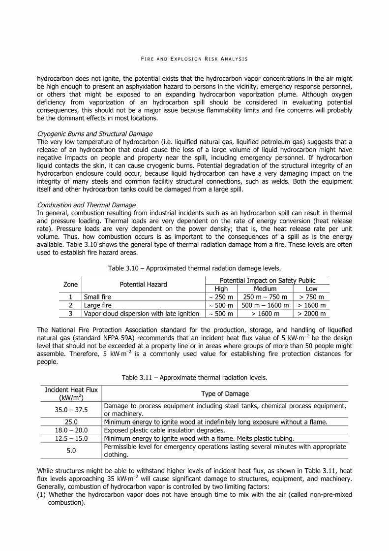
FF II RR EE AA NN DD EE XX PP LL OO SS II OO NN RR II SS KK AA NN AA LL YY SS II SS
hydrocarbon does not ignite, the potential exists that the hydrocarbon vapor concentrations in the air might be high enough to present an asphyxiation hazard to persons in the vicinity, emergency response personnel, or others that might be exposed to an expanding hydrocarbon vaporization plume. Although oxygen deficiency from vaporization of an hydrocarbon spill should be considered in evaluating potential consequences, this should not be a major issue because flammability limits and fire concerns will probably be the dominant effects in most locations. Cryogenic Burns and Structural Damage The very low temperature of hydrocarbon (i.e. liquified natural gas, liquified petroleum gas) suggests that a release of an hydrocarbon that could cause the loss of a large volume of liquid hydrocarbon might have negative impacts on people and property near the spill, including emergency personnel. If hydrocarbon liquid contacts the skin, it can cause cryogenic burns. Potential degradation of the structural integrity of an hydrocarbon enclosure could occur, because liquid hydrocarbon can have a very damaging impact on the integrity of many steels and common facilitiy structural connections, such as welds. Both the equipment itself and other hydrocarbon tanks could be damaged from a large spill. Combustion and Thermal Damage In general, combustion resulting from industrial incidents such as an hydrocarbon spill can result in thermal and pressure loading. Thermal loads are very dependent on the rate of energy conversion (heat release rate). Pressure loads are very dependent on the power density; that is, the heat release rate per unit volume. Thus, how combustion occurs is as important to the consequences of a spill as is the energy available. Table 3.10 shows the general type of thermal radiation damage from a fire. These levels are often used to establish fire hazard areas.
Table 3.10 – Approximated thermal radation damage levels.
PPootteennttiiaall IImmppaacctt oonn SSaaffeettyy PPuubblliicc ZZoonnee PPootteennttiiaall HHaazzaarrdd HHiigghh MMeeddiiuumm LLooww
1 Small fire 250 m 250 m – 750 m > 750 m 2 Large fire 500 m 500 m – 1600 m > 1600 m 3 Vapor cloud dispersion with late ignition 500 m > 1600 m > 2000 m
The National Fire Protection Association standard for the production, storage, and handling of liquefied natural gas (standard NFPA-59A) recommends that an incident heat flux value of 5 kWm2 be the design level that should not be exceeded at a property line or in areas where groups of more than 50 people might assemble. Therefore, 5 kWm2 is a commonly used value for establishing fire protection distances for people.
Table 3.11 – Approximate thermal radiation levels.
IInncciiddeenntt HHeeaatt FFlluuxx ((kkWW//mm22)) TTyyppee ooff DDaammaaggee
35.0 – 37.5 Damage to process equipment including steel tanks, chemical process equipment, or machinery.
25.0 Minimum energy to ignite wood at indefinitely long exposure without a flame. 18.0 – 20.0 Exposed plastic cable insulation degrades. 12.5 – 15.0 Minimum energy to ignite wood with a flame. Melts plastic tubing.
5.0 Permissible level for emergency operations lasting several minutes with appropriate clothing.
While structures might be able to withstand higher levels of incident heat flux, as shown in Table 3.11, heat flux levels approaching 35 kWm2 will cause significant damage to structures, equipment, and machinery. Generally, combustion of hydrocarbon vapor is controlled by two limiting factors: (1) Whether the hydrocarbon vapor does not have enough time to mix with the air (called non-pre-mixed
combustion).

FF II RR EE AA NN DD EE XX PP LL OO SS II OO NN FF UU NN DD AA MM EE NN TT AA LL AA NN AA LL YY SS II SS
(2) Whether the ignition occurs after the fuel has time to mix with the surrounding air (appropriately called
pre-mixed combustion). Therefore, ignition time is important in spill scenarios to assess appropriately the type and extent of thermal radiation from an hydrocarbon spill and fire. As noted in Table 3.11, combustion and thermal damage from a fire can have severe consequences and should be carefully and thoroughly analyzed.
Hydrocarbon Fireballs Two types of combustion modes might produce damaging pressure: deflagration and detonation. Deflagration is a rapid combustion that progresses through an unburned fuel and air mixture at subsonic velocities; whereas, detonation is an extremely rapid combustion that progresses through an unburned fuel and air mixture at supersonic velocities. For low reactivity fuels such as natural gas, combustion will usually progress at low velocities and will not generate significant overpressure under normal conditions. Ignition of a vapor cloud will cause the vapor to burn back to the spill source. This is generally referred to as a fireball, which, by its nature, generates relatively low pressures, thus having a low potential for pressure damage to structures. Hydrocarbon and Air Mixture Explosions Certain conditions, however, might cause an increase in burn rate that does result in overpressure. If the fuel and air mixture cloud is confined (e.g. trapped between obstacles), is very turbulent as it progresses through or around obstacles, or encounters a high-pressure ignition source, a rapid acceleration in burn rate might occur. The potential for damaging overpressures from such events could occur under some limited spill and dispersion scenarios, specifically in confined areas. However, effects will be localized near the hydrocarbon spill source and are not expected to cause extensive structural damage. Rapid Phase Transitions (RPT) Rapid phase transitions occur when the temperature difference between a hot liquid and a cold liquid is sufficient to drive the cold liquid rapidly to its superheat limit, resulting in spontaneous and explosive boiling of the cold liquid. When a cryogenic liquid such as hydrocarbon is suddenly heated by contacting a warm liquid such as water, explosive boiling of the hydrocarbon can occur, resulting in localized overpressure releases. Energy releases equivalent to several kilograms of high explosive have been observed. The impacts of this phenomenon will be localized near the hydrocarbon spill source and should not cause extensive structural damage. EE VV AA LL UU AA TT II OO NN OO FF FF OO UU RR RR EE CC EE NN TT HH YY DD RR OO CC AA RR BB OO NN SS PP II LL LL MM OO DD EE LL II NN GG SS TT UU DD II EE SS Four recent hydrocarbon spill modeling studies were evaluated to assess whether they provide a definitive determination of the lateral extent and thermal hazards of a large scale release of hydrocarbon over water. The results of the comparisons are summarized below in Table 3.12. The studies reviewed include: (1) Comparison of Hypothetical LNG and Fuel Oil Fires on Water. Report by the National Oceanic and
Atmospheric Administration (NOAA), Office of Response and Restoration, Seattle, WA, Lehr and Simicek-Beatty, 2003.
(2) Model of spills and fires from LNG and oil tankers. Journal of Hazardous Materials, B96-2003, 171-188, Fay, 2003.
(3) Modeling LNG Spills in Boston Harbor. Quest Consultants, Inc., 908 26th Ave N.W., Norman, OK 73609; Letter from Quest Consultants to Department of Energy (October 2, 2001), Letter from Quest Consultants to Department of Energy (October 3, 2001); and Letter from Quest Consultants to Department of Energy (November 17, 2003).
(4) Liquefied Natural Gas in Vallejo: Health and Safety Issues. LNG Health and Safety Committee of the Disaster Council of the City of Vallejo, CA, January, 2003.
An event tree of generic hydrocarbon spill scenarios was used to compare and contrast the analysis process in each study. Table 3.12 presents a summary of the hydrocarbon spill and fire hazard predictions for each of the studies. The distances between the fuel fire and specific thermal hazards are shown in the columns labeled as “Skin Burn Distance” and “Paper Ignition Distance.” A secondary indicator of thermal hazard is shown in the “Fire Duration” column. All the studies assumed ignition such that the fuel burns as a pool fire, with no explosions.
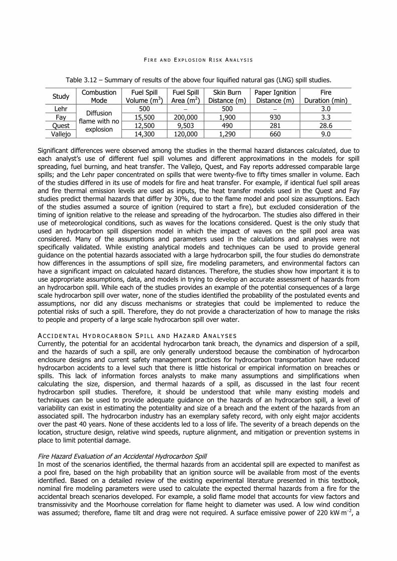
FF II RR EE AA NN DD EE XX PP LL OO SS II OO NN RR II SS KK AA NN AA LL YY SS II SS
Table 3.12 – Summary of results of the above four liquified natural gas (LNG) spill studies.
SSttuuddyy CCoommbbuussttiioonn MMooddee
FFuueell SSppiillll VVoolluummee ((mm33))
FFuueell SSppiillll AArreeaa ((mm22))
SSkkiinn BBuurrnn DDiissttaannccee ((mm))
PPaappeerr IIggnniittiioonn DDiissttaannccee ((mm))
FFiirree DDuurraattiioonn ((mmiinn))
Lehr 500 500 3.0 Fay 15,500 200,000 1,900 930 3.3
Quest 12,500 9,503 490 281 28.6 Vallejo
Diffusion flame with no
explosion 14,300 120,000 1,290 660 9.0
Significant differences were observed among the studies in the thermal hazard distances calculated, due to each analyst’s use of different fuel spill volumes and different approximations in the models for spill spreading, fuel burning, and heat transfer. The Vallejo, Quest, and Fay reports addressed comparable large spills; and the Lehr paper concentrated on spills that were twenty-five to fifty times smaller in volume. Each of the studies differed in its use of models for fire and heat transfer. For example, if identical fuel spill areas and fire thermal emission levels are used as inputs, the heat transfer models used in the Quest and Fay studies predict thermal hazards that differ by 30%, due to the flame model and pool size assumptions. Each of the studies assumed a source of ignition (required to start a fire), but excluded consideration of the timing of ignition relative to the release and spreading of the hydrocarbon. The studies also differed in their use of meteorological conditions, such as waves for the locations considered. Quest is the only study that used an hydrocarbon spill dispersion model in which the impact of waves on the spill pool area was considered. Many of the assumptions and parameters used in the calculations and analyses were not specifically validated. While existing analytical models and techniques can be used to provide general guidance on the potential hazards associated with a large hydrocarbon spill, the four studies do demonstrate how differences in the assumptions of spill size, fire modeling parameters, and environmental factors can have a significant impact on calculated hazard distances. Therefore, the studies show how important it is to use appropriate assumptions, data, and models in trying to develop an accurate assessment of hazards from an hydrocarbon spill. While each of the studies provides an example of the potential consequences of a large scale hydrocarbon spill over water, none of the studies identified the probability of the postulated events and assumptions, nor did any discuss mechanisms or strategies that could be implemented to reduce the potential risks of such a spill. Therefore, they do not provide a characterization of how to manage the risks to people and property of a large scale hydrocarbon spill over water. AA CC CC II DD EE NN TT AA LL HH YY DD RR OO CC AA RR BB OO NN SS PP II LL LL AA NN DD HH AA ZZ AA RR DD AA NN AA LL YY SS EE SS Currently, the potential for an accidental hydrocarbon tank breach, the dynamics and dispersion of a spill, and the hazards of such a spill, are only generally understood because the combination of hydrocarbon enclosure designs and current safety management practices for hydrocarbon transportation have reduced hydrocarbon accidents to a level such that there is little historical or empirical information on breaches or spills. This lack of information forces analysts to make many assumptions and simplifications when calculating the size, dispersion, and thermal hazards of a spill, as discussed in the last four recent hydrocarbon spill studies. Therefore, it should be understood that while many existing models and techniques can be used to provide adequate guidance on the hazards of an hydrocarbon spill, a level of variability can exist in estimating the potentiality and size of a breach and the extent of the hazards from an associated spill. The hydrocarbon industry has an exemplary safety record, with only eight major accidents over the past 40 years. None of these accidents led to a loss of life. The severity of a breach depends on the location, structure design, relative wind speeds, rupture alignment, and mitigation or prevention systems in place to limit potential damage. Fire Hazard Evaluation of an Accidental Hydrocarbon Spill In most of the scenarios identified, the thermal hazards from an accidental spill are expected to manifest as a pool fire, based on the high probability that an ignition source will be available from most of the events identified. Based on a detailed review of the existing experimental literature presented in this textbook, nominal fire modeling parameters were used to calculate the expected thermal hazards from a fire for the accidental breach scenarios developed. For example, a solid flame model that accounts for view factors and transmissivity and the Moorhouse correlation for flame height to diameter was used. A low wind condition was assumed; therefore, flame tilt and drag were not required. A surface emissive power of 220 kWm2, a
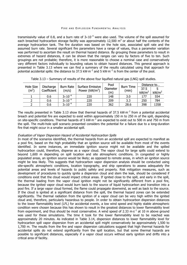
FF II RR EE AA NN DD EE XX PP LL OO SS II OO NN FF UU NN DD AA MM EE NN TT AA LL AA NN AA LL YY SS II SS
transmissivity value of 0.8, and a burn rate of 3104 were also used. The volume of the spill assumed for each breached hydrocarbon storage facility was approximately 12,500 m3 or about half the contents of the average hydrocarbon tank. The fire duration was based on the hole size, associated spill rate and the assumed burn rate. Several significant fire parameters have a range of values, thus a parameter variation was performed to ascertain the result on thermal hazard distance. By grouping these parameters to result in extremes of hazard distances, it can be shown that the ranges can vary by factors of five to ten. Such groupings are not probable; therefore, it is more reasonable to choose a nominal case and conservatively vary different factors individually to bounding values to obtain hazard distances. This general approach is presented in Table 3.13 where we can find a summary of the results calculated using that approach for potential accidental spills: the distance to 37.5 kWm2 and 5 kWm2 is from the center of the pool.
Table 3.13 – Summary of results of the above four liquified natural gas (LNG) spill studies.
DDiissttaannccee ttoo…… HHoollee SSiizzee ((mm22))
DDiisscchhaarrggee CCooeeffffiicciieenntt
BBuurrnn RRaattee ((mm//ss))
SSuurrffaaccee EEmmiissssiivvee PPoowweerr ((kkWW//mm22))
PPooooll DDiiaammeetteerr
((mm))
BBuurrnn TTiimmee ((mmiinn)) 3377..55
kkWW//mm22 55
kkWW//mm22 1 0.6 3104 220 148 3.0 177 554 2 0.6 3104 220 209 3.3 250 784 2 0.6 3104 220 362 28.6 398 1358
The results presented in Table 3.13 show that thermal hazards of 37.5 kWm2 from a potential accidental breach and potential fire are expected to exist within approximately 150 m to 250 m of the spill, depending on site-specific conditions. Thermal hazards of 5 kWm2 are expected to exist out to 500 m and 750 m from the spill. The multi-hole spill scenario presented considers the potential for a failure due to a long-duration fire that might occur in a smaller accidental spill. Evaluation of Vapor Dispersion Hazard of Accidental Hydrocarbon Spills In most of the scenarios identified, the thermal hazards from an accidental spill are expected to manifest as a pool fire, based on the high probability that an ignition source will be available from most of the events identified. In some instances, an immediate ignition source might not be available and the spilled hydrocarbon could, therefore, disperse as a vapor cloud. The vapor cloud for large spills could extend to beyond 1,600 m depending on spill location and site atmospheric conditions. In congested or highly populated areas, an ignition source would be likely; as opposed to remote areas, in which an ignition source might be less likely. This suggests that hydrocarbon vapor dispersion analysis should be conducted using site-specific atmospheric conditions, location topography, and ship operations to assess adequately the potential areas and levels of hazards to public safety and property. Risk mitigation measures, such as development of procedures to quickly ignite a dispersion cloud and stem the leak, should be considered if conditions exist that the cloud would impact critical areas. If ignited close to the spill, and early in the spill, the thermal loading from the vapor cloud ignition might not be significantly different from a pool fire, because the ignited vapor cloud would burn back to the source of liquid hydrocarbon and transition into a pool fire. If a large vapor cloud formed, the flame could propagate downwind, as well as back to the source. If the cloud is ignited at a significant distance from the spill, the thermal hazard zones can be extended significantly. The thermal radiation from the ignition of a vapor cloud can be very high within the ignited cloud and, therefore, particularly hazardous to people. In order to obtain hydrocarbon dispersion distances to the lower flammability level (LFL) for accidental events, a low wind speed and highly stable atmospheric condition were chosen because this has shown to result in the greatest distances to lower flammability level from experiment, and thus should be most conservative. A wind speed of 2.33 ms1 at 10 m above ground was used for these simulations. The time it took for the lower flammability level to be reached was approximately 20 minutes. As indicated in Table 3.14, dispersion distances to lower flammability level for hydrocarbon spill vapor dispersion from an accidental spill might conservatively be approximately 1,500 to 1,700 m. The results from the fire and vapor dispersion calculations suggest that high thermal hazards for accidental spills do not extend significantly from the spill location, but that some thermal hazards are possible to significant distances, especially if a vapor cloud occurs without early ignition and drifts into a critical area of facility.

FF II RR EE AA NN DD EE XX PP LL OO SS II OO NN RR II SS KK AA NN AA LL YY SS II SS
Table 3.14 – Dispersion distances to lower flammability level (LFL) for accidental spills.
HHoollee SSiizzee ((mm22))
SSppiillll DDuurraattiioonn ((mmiinn))
PPooooll DDiiaammeetteerr ((mm))
DDiissttaannccee ttoo LLFFLL ((mm))
1 40 148 1,536 2 20 209 1,710
Table 3.15 summarizes the estimated results of the impact on public safety and property for an accidental breach and spill. In this table, high impact would include a thermal intensity in the range of 37.5 kWm2 and low values would correspond to thermal intensities in the range of 5 kWm2.
Table 3.15 – Approximated impact of accidental breaches and spills on public safety and property.
PPootteennttiiaall IImmppaacctt oonn SSaaffeettyy PPuubblliicc PPootteennttiiaall HHaazzaarrdd 225500 mm 225500 mm –– 775500 mm >> 775500 mm
Small fire High Medium Low Vapor cloud High High or medium Medium Big fire High High Medium
Where very low impact signifies little or no property damage or injuries, low impact represents a minor property damage and minor injuries, medium impact stands for potential for injuries and property damage, and high impact reveals major injuries and significant damage to structures. II NN TT EE NN TT II OO NN AA LL HH YY DD RR OO CC AA RR BB OO NN SS PP II LL LL AA NN DD HH AA ZZ AA RR DD AA NN AA LL YY SS EE SS Currently, the potential for an intentional hydrocarbon enclosure breach, the dynamics and dispersion of a large spill, and the hazards of such a spill, are not fully understood, for two primary reasons. First, the combination of hydrocarbon enclosure designs and current safety management practices for hydrocarbon transportation have reduced hydrocarbon accidents, so that there is little historical or empirical information on large breaches or spills. Second, for an intentional event, existing experimental data on hydrocarbon spill dynamics, dispersion, and burning over water cover spill volumes that are more than two orders of magnitude less than the spill volumes being postulated in many recent studies. This lack of information forces analysts to make many assumptions and simplifications when calculating the size, dispersion, and thermal hazards of a spill. Determination of the potential or likelihood of such an event depends on the breach scenario, the spill location, and any implementation of prevention and mitigation strategies to prevent such an event. In areas where cascading failures might be a significant issue, the use of complex, coupled, thermal, fluid and structural analyses should be considered to improve the analysis of the potential for and extent of structural damage hydrocarbon facilities. Evaluation of the Fire Hazard of an Intentional Hydrocarbon Spill In most of the scenarios identified, the thermal hazards from an intentional spill are expected to manifest as a pool fire, based on the high probability that an ignition source will be available from most of the events identified. Based on a detailed review of the existing experimental literature, nominal fire modeling parameters were used to calculate the expected thermal hazards from a fire for the intentional breach scenarios developed. In Table 3.16 a summary of these results is shown where the distances to 37.5 kWm2 and 5 kWm2 are from the center of the pool. The results presented in Table 3.16 show that the thermal hazards of 37.5 kWm2 are expected to occur within approximately 500 m of the spill for most of the scenarios evaluated. For the 2 m2 three-hole breach, it was assumed that individual pools would form; whereas, for the 5 m2 three-hole breach, a single pool was assumed to form. Most of the studies reviewed assume that a single, coherent pool fire can be maintained for very large pool diameters. This would be unlikely due to the inability of air to reach the interior of a fire and maintain combustion on an hydrocarbon pool that size. Instead, the flame pool envelope would break up into multiple pool fires (herein “flamelets”), the heights of which are much less than the fuel bed diameter used in the calculations by the four previously discussed studies. This breakup into flamelets results in a much shorter flame height than that assumed for a large pool diameter. In reality, flame height-to-pool diameter ratio (L/D) would probably be much smaller than that assumed by the correlations in many studies, which predict an flame height-to-pool diameter ratio ratio between 1.0 and 2.0. A more realistic ratio could be less than 1.0.

FF II RR EE AA NN DD EE XX PP LL OO SS II OO NN FF UU NN DD AA MM EE NN TT AA LL AA NN AA LL YY SS II SS
Table 3.16 – Summary of results of the above four liquified natural gas (LNG) spill studies.
DDiissttaannccee ttoo…… HHoollee SSiizzee ((mm22))
DDiisscchhaarrggee CCooeeffffiicciieenntt
BBuurrnn RRaattee ((mm//ss))
SSuurrffaaccee EEmmiissssiivvee PPoowweerr ((kkWW//mm22))
PPooooll DDiiaammeetteerr
((mm))
BBuurrnn TTiimmee ((mmiinn)) 3377..55
kkWW//mm22 55
kkWW//mm22 1 0.6 3104 220 148 3.0 177 554 2 0.6 3104 220 209 3.3 250 784 5 0.6 3104 350 330 8.1 529 1,652 12 0.6 3104 220 512 3.4 602 1,920
Because the heat radiated by the flamelets would be far less than the heat radiation calculated in the many studies (based on a large pool fire), the amount of radiative heat flux that an adjacent object receives would be less, thereby decreasing the size of the thermal hazard zone. The development of fire whirls might increase the hazard zone. Therefore, this type of pool fire model should be carefully considered to improve thermal hazards analysis from potential large spills. The results presented suggest that the potential thermal hazards for large spills can vary significantly, based on the uncertainty associated with potential spill sizes, dispersion variations, and threats. Based on the estimated pool size for large spills, even with the possibility of reduction in effects for mass fires as opposed to single pool fires, high thermal hazards approaching 37.5 kWm2 could probably extend to approximately 500 meters. The thermal hazards between 500 meters and 1,600 meters decrease significantly. The hazards would be low, approximately 5 kWm2 beyond 1,600 m from even a large spill. Based on these observations, approximate hazard zones seem to exist between 0 m to 500 m, 500 m to 1,600 m, and over 1,600 m, and were used to develop guidance on managing risks for hydrocarbon spills. Evaluation of Vapor Dispersion Hazard of Intentional Hydrocarbon Spills In most of the scenarios identified, the thermal hazards from a spill are expected to manifest as a pool fire, based on the high probability that an ignition source will be available from most of the events identified. In some instances, such as an intentional spill without a tank breach, an immediate ignition source might not be available and the spilled hydrocarbon could, therefore, disperse as a vapor cloud. For large spills, the vapor cloud could extend to more than 1,600 meters, depending on spill location and site atmospheric conditions. In congested or highly populated areas, an ignition source would be likely, as opposed to remote areas, in which an ignition source might be less likely. The impact from a vapor cloud dispersion and ignition from a large spill can extend beyond 1,600 meters. This suggests that hydrocarbon vapor dispersion analysis shoul be conducted using site-specific atmospheric conditions, location topography, and operations to assess adequately the potential areas and levels of hazards to public safety and property. Consideration of risk mitigation measures, such as development of procedures to quickly ignite a dispersion cloud and stem the leak, if conditions exist that the cloud would impact critical areas. If ignited close to the spill, and early in the spill, the thermal loading from the vapor cloud ignition might not be significantly different from a pool fire, because the ignited vapor cloud would burn back to the source of liquid hydrocarbon and transition into a pool fire. If a large vapor cloud formed, the flame could propagate downwind, as well as back to the source. If the cloud is ignited at a significant distance from the spill, the thermal hazard zones can be extended significantly. The thermal radiation from the ignition of a vapor cloud can be very high within the ignited cloud and, therefore, particularly hazardous to people. A low wind speed and highly stable atmospheric condition were chosen because this state has shown to result in the greatest distances to lower flammability level (LFL) from experiment, and thus should be the most conservative. A wind speed of 2.33 ms1 at 10 m above ground was used for these simulations. While previous studies have addressed the vapor dispersion issue from a consequence standpoint only, the risk analysis performed as part of this study indicates that the potential for a large vapor dispersion from an intentional breach is highly unlikely. This is due to the high probability that an ignition source will be available for many of the initiating events identified, and because certain risk reduction techniques can be applied to prevent or mitigate the initiating events identified. The significant distances, though, of a potential vapor dispersion suggest that hydrocarbon vapor dispersion analysis and risk mitigation measures should be carefully considered to protect adequately both the public and property.

FF II RR EE AA NN DD EE XX PP LL OO SS II OO NN RR II SS KK AA NN AA LL YY SS II SS
Table 3.17 – Dispersion distances to lower flammability level (LFL) for accidental spills.
HHoollee SSiizzee ((mm22))
SSppiillll DDuurraattiioonn ((mmiinn))
PPooooll DDiiaammeetteerr ((mm))
DDiissttaannccee ttoo LLFFLL ((mm))
5 8.1 330 2,450 5 8.1 572 3,614
The analyses from the fire and vapor dispersion calculations suggest that high thermal hazards from intentional events extend significantly from the spill location. Table 3.18 summarizes the general impacts on both public safety and property for intentional breaches and spills. In this table, high impact would include a thermal intensity in the range of 37.5 kWm2 and low values would correspond to thermal intensities in the range of 5 kWm2 . These results should be used as guidance, bearing in mind that these distances will vary, based on site-specific factors and environmental conditions.
Table 3.18 – Approximated impact of accidental breaches and spills on public safety and property.
PPootteennttiiaall IImmppaacctt oonn SSaaffeettyy PPuubblliicc PPootteennttiiaall HHaazzaarrdd 550000 mm 550000 mm –– 116600 mm >> 11660000 mm
Small fire High Medium Low Fireball Medium Low Very low Vapor cloud High High or medium Medium Big fire High High Medium
Where very low impact signifies little or no property damage or injuries, low impact represents a minor property damage and minor injuries, medium impact stands for potential for injuries and property damage, and high impact reveals major injuries and significant damage to structures. RR II SS KK MM AA NN AA GG EE MM EE NN TT SS TT RR AA TT EE GG II EE SS (( PP RR EE VV EE NN TT II OO NN AA NN DD MM II TT II GG AA TT II OO NN )) Many factors can impact risks to public safety and property from an hydrocarbon spill: design, materials selection, manufacturing methods, inspection and testing, assembly techniques, worker training, and safety operations, among others. Other significant factors include terminal location and design, port handling elements (e.g. tugboats and firefighting equipment), communications systems, and emergency response capabilities. It is important to realize that a decision involving large capital expense can have long-lasting effects (e.g. hydrocarbon terminal site selection). For this reason, it is imperative to consider carefully all risk management decisions in order that residual or future risks can be managed to an acceptable level. In general, risk can be managed by prevention or mitigation. Prevention seeks to avoid an accident or attack; mitigation reduces the effects of an accident or attack. While the prevention and mitigation strategies identified are possible, many might not be cost-effective or even practical in certain locations or applications. Risk management should be based on developing or combining approaches that can be effectively and efficiently implemented to reduce hazards to acceptable levels in a cost-effective manner. This type of approach has been in use and is in use by the hydrocarbon industry, and public safety organizations to ensure the safety of the transportation of hydrocarbon. These efforts include a number of design, construction, safety equipment, and operational efforts to reduce the potential for an hydrocarbon spill. While risks can seldom be reduced to zero, prevention of the higher consequence events can significantly reduce hazards to public safety and property and facilitate mitigation of the remaining lower consequence and lower risk events. Prevention and mitigation strategy implementation should key on effectiveness, costs, and operational impacts. The level of risk reduction required should be determined in conjunction with local public officials and public safety organizations such as police and fire departments, emergency response services, port authorities, and other appropriate stakeholders. Risk reduction strategies that are effective at one site might not be effective at another site, and should be considered in the context of how a risk management approach might be customized to yield benefits to public safety and property while having limited operational impacts. Application of the Risk Management Process So far, in this section we have discussed risk reduction for areas or activities within the larger system that includes neighboring infrastructures. We used the risk management guidance and safety information

FF II RR EE AA NN DD EE XX PP LL OO SS II OO NN FF UU NN DD AA MM EE NN TT AA LL AA NN AA LL YY SS II SS
developed in this text to assess ways to enhance operations and reduce the potential risks to the public. Hopefully, this will provide the reader with suggestions on how to consider various issues, including terminal location and site conditions, operational conditions, environmental effects, and safety and security concerns and measures. To be feasible, such a process must be effective from a surety standpoint, affordable, possible to implement in a timely fashion, minimize environmental impact, and be otherwise amenable to regulators and stakeholders. We are not intending to suggest a “cookbook” methodology for selecting new sites; however, we want the reader to understand what type of issues should be considered and what various measures should be applied to try to achieve appropriate levels of protection of public safety and property for hydrocarbon imports. Applying the Risk Management Process Risk management of an hydrocarbon facility should be viewed as a system that includes the nearest neighbors along the hydrocarbon storage and handling equipment. Four classes of attributes affect the overall risks. These include: (1) The context of the hydrocarbon facility – location, site specific conditions, hydrocarbon terminal,
importance to the region; (2) Potential targets and threats – potential accidental events, credible intentional events, and infrastructure
targets; (3) Risk management goals – identification of levels of consequences to be avoided, such as injuries and
property damage, hydrocarbon supply reliability required; (4) Protection system capabilities – hydrocarbon tanker safety and security measures, hydrocarbon
operations safety and security measures, and early warning and emergency response or recovery measures.
In the risk management process the four attributes discussed are then evaluated to determine if the protection system in place can effectively meet the risk management goals identified for a specific import terminal site and operations. If so, then the safety and security measures and operations developed for the hydrocarbon operations are adequate. Hydrocarbon operations should be reviewed on a regular basis to assess whether changes in context, targets or threats, risk management goals or risk management systems have changed such that a reassessment of risks is needed. If the initial risk assessment determines that the identified risk management goals are not being met, then potential modifications in location and site conditions, hydrocarbon operations, safety and security measures, emergency response and early warning measures should be assessed to determine effective improvements in the overall risk management system Below, we provide a summary of the elements that should be considered for hydrocarbon facility applications for each step of the risk management process identified. These steps provide a context of how the safety analysis and risk guidance provided in this report can be used to evaluate options to protect property and public health and safety associated with hydrocarbon operations. Characterize Assets – In this step, the context of the hydrocarbon facility such as location, site-specific conditions, and nominal operations should be identified and developed. Information that should be collected and considered includes: (1) Type and Proximity of Neighbors – Distance to residential, commercial, and industrial facilities or other
critical infrastructures such as bridges or tunnels. (2) Environmental Conditions – Wind-driven spill movement and dispersion (prevailing wind direction, speed,
and variability), severe weather considerations (hurricanes, storm surges), tidal-driven spill movement and dispersion (height, current, and influence on spill movement and dispersion), seismic issues (ground displacement, soil liquefaction), temperature issues (ice, thermal impediment to operations).
(3) Nominal Operational Conditions – Available storage, seasonal demands, percentage of regional or local supply, additional traffic (near other large ships, pleasure boats) and distance to it, transit near critical infrastructures (such as other terminals, commercial areas, or residential areas), number of critical facilities along transit, and distance to critical facilities along transit.
Identify Potential Threats – In this step, the potential or likely threats expected for the facility, based on site location and relative attractiveness of either an hydrocarbon facility or other nearby targets, should be identified:
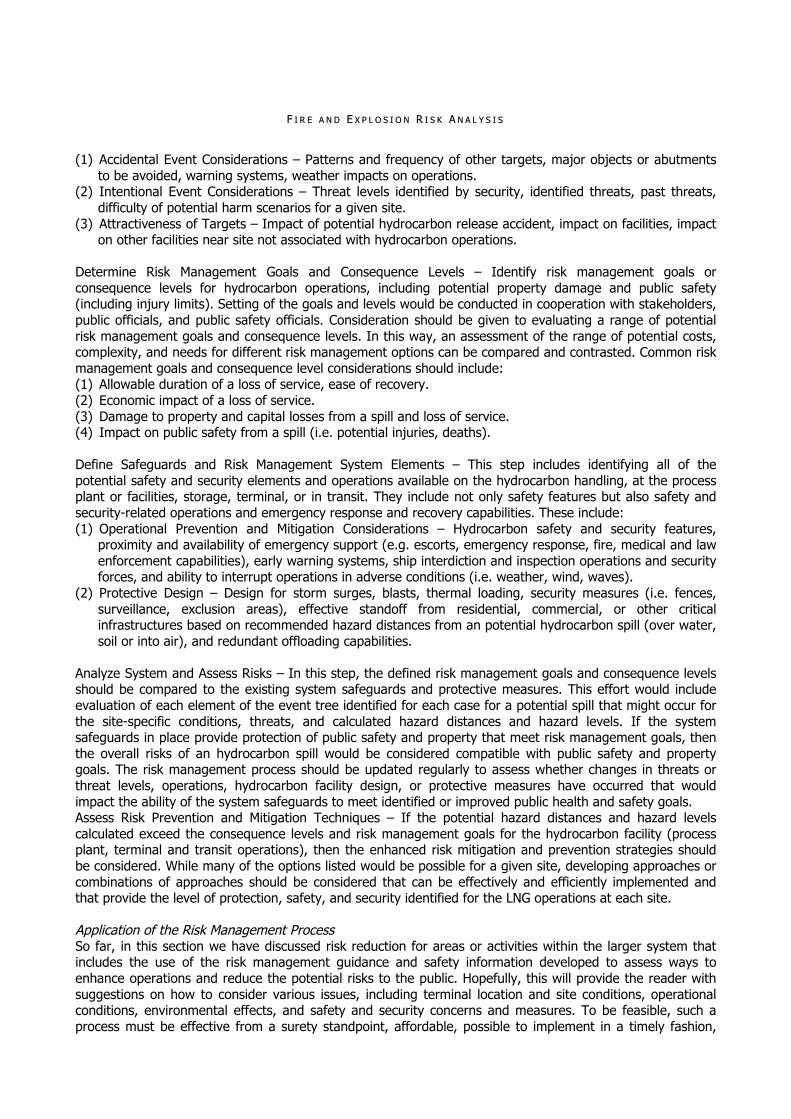
FF II RR EE AA NN DD EE XX PP LL OO SS II OO NN RR II SS KK AA NN AA LL YY SS II SS
(1) Accidental Event Considerations – Patterns and frequency of other targets, major objects or abutments to be avoided, warning systems, weather impacts on operations.
(2) Intentional Event Considerations – Threat levels identified by security, identified threats, past threats, difficulty of potential harm scenarios for a given site.
(3) Attractiveness of Targets – Impact of potential hydrocarbon release accident, impact on facilities, impact on other facilities near site not associated with hydrocarbon operations.
Determine Risk Management Goals and Consequence Levels – Identify risk management goals or consequence levels for hydrocarbon operations, including potential property damage and public safety (including injury limits). Setting of the goals and levels would be conducted in cooperation with stakeholders, public officials, and public safety officials. Consideration should be given to evaluating a range of potential risk management goals and consequence levels. In this way, an assessment of the range of potential costs, complexity, and needs for different risk management options can be compared and contrasted. Common risk management goals and consequence level considerations should include: (1) Allowable duration of a loss of service, ease of recovery. (2) Economic impact of a loss of service. (3) Damage to property and capital losses from a spill and loss of service. (4) Impact on public safety from a spill (i.e. potential injuries, deaths). Define Safeguards and Risk Management System Elements – This step includes identifying all of the potential safety and security elements and operations available on the hydrocarbon handling, at the process plant or facilities, storage, terminal, or in transit. They include not only safety features but also safety and security-related operations and emergency response and recovery capabilities. These include: (1) Operational Prevention and Mitigation Considerations – Hydrocarbon safety and security features,
proximity and availability of emergency support (e.g. escorts, emergency response, fire, medical and law enforcement capabilities), early warning systems, ship interdiction and inspection operations and security forces, and ability to interrupt operations in adverse conditions (i.e. weather, wind, waves).
(2) Protective Design – Design for storm surges, blasts, thermal loading, security measures (i.e. fences, surveillance, exclusion areas), effective standoff from residential, commercial, or other critical infrastructures based on recommended hazard distances from an potential hydrocarbon spill (over water, soil or into air), and redundant offloading capabilities.
Analyze System and Assess Risks – In this step, the defined risk management goals and consequence levels should be compared to the existing system safeguards and protective measures. This effort would include evaluation of each element of the event tree identified for each case for a potential spill that might occur for the site-specific conditions, threats, and calculated hazard distances and hazard levels. If the system safeguards in place provide protection of public safety and property that meet risk management goals, then the overall risks of an hydrocarbon spill would be considered compatible with public safety and property goals. The risk management process should be updated regularly to assess whether changes in threats or threat levels, operations, hydrocarbon facility design, or protective measures have occurred that would impact the ability of the system safeguards to meet identified or improved public health and safety goals. Assess Risk Prevention and Mitigation Techniques – If the potential hazard distances and hazard levels calculated exceed the consequence levels and risk management goals for the hydrocarbon facility (process plant, terminal and transit operations), then the enhanced risk mitigation and prevention strategies should be considered. While many of the options listed would be possible for a given site, developing approaches or combinations of approaches should be considered that can be effectively and efficiently implemented and that provide the level of protection, safety, and security identified for the LNG operations at each site. Application of the Risk Management Process So far, in this section we have discussed risk reduction for areas or activities within the larger system that includes the use of the risk management guidance and safety information developed to assess ways to enhance operations and reduce the potential risks to the public. Hopefully, this will provide the reader with suggestions on how to consider various issues, including terminal location and site conditions, operational conditions, environmental effects, and safety and security concerns and measures. To be feasible, such a process must be effective from a surety standpoint, affordable, possible to implement in a timely fashion,

FF II RR EE AA NN DD EE XX PP LL OO SS II OO NN FF UU NN DD AA MM EE NN TT AA LL AA NN AA LL YY SS II SS
minimize environmental impact, and be otherwise amenable to regulators and stakeholders. We are not intending to suggest a “cookbook” methodology for selecting new sites; however, we want the reader to understand what type of issues should be considered and what various measures should be applied to try to achieve appropriate levels of protection (LOP) of public safety and property for hydrocarbon handling. Risk management of an hydrocarbon facility should be viewed as a system that includes the hydrocarbon process operations, terminal facilities and location, the transit path (including waterways), and the nearest neighbors along the transit path and at the terminals. Four classes of attributes affect the overall risks. These include: (1) The context of the hydrocarbon facility – Location, site specific conditions, importance to the region; (2) Potential targets and threats – Potential accidental events, credible intentional events, and ship or
infrastructure targets; (3) Risk management goals – Identification of levels of consequences to be avoided, such as injuries and
property damage, hydrocarbon supply reliability required; (4) Protection system capabilities – Hydrocarbon facility safety and security measures, hydrocarbon
operations safety and security measures, and early warning and emergency response and recovery measures.
In the risk management process, the four attributes discussed are then evaluated to determine if the protection system in place can effectively meet the risk management goals identified for a specific hydrocarbon facility site and operations. If so, then the safety and security measures and operations developed for the hydrocarbon operations are adequate. Import operations should be reviewed on a regular basis to assess whether changes in context, targets or threats, risk management goals or risk management systems have changed such that a reassessment of risks is needed. If the initial risk assessment determines that the identified risk management goals are not being met, then potential modifications in location and site conditions, safety and security measures, emergency response and early warning measures should be assessed to determine effective improvements in the overall risk management system.
HH YY DD RR OO CC AA RR BB OO NN SS PP II LL LL AA NN DD DD II SS PP EE RR SS II OO NN AA NN AA LL YY SS II SS Several models have been developed for the spread of hydrocarbon on water (Fay, 1973). For confined and unconfined water surfaces, the usually model assumes that boiling occurs in the film-boiling mode. Instantaneous and continuous spills that included the effect of mass and heat transfer, shear forces, and surface tension were modeled. Pool break-up was accounted for by including the effect of shear forces and surface tension. It was found that the time necessary to reach a steady-state radius for continuous spills increased as surface shear stress increased. The steady-state pool radius was not affected. Spreading is driven by gravity. PP OO OO LL BB OO II LL II NN GG Boe performed laboratory scale experiments with liquefied methane-ethane and methanepropane mixtures boiling on water (Boe, 1998). The results indicated that addition of ethane or propane affects the boil-off rate. High initial boil-off rates were observed for methane rich mixtures similar to that of typical liquified natural gas (LNG) compositions. The boil-off rates increased by a factor of 1.5 to 2.0 from that of pure methane, when either ethane or propane was added to methane to obtain a 97% methane mixture. It was concluded that there is a breakdown of film boiling due to closer contact between the mixture and water, causing a higher heat flux and lower surface temperature below that to maintain a continuous vapor film. On laboratory scale experiments showed that liquified natural gas had a higher boiling rate than pure methane on a bound-free surface. The rate of boiling increased with time and foaming of the liquified natural gas occurred on the water surface. Spreading based upon a gravitational-inertia balance, heat transfer, and vaporization pointed out that preferential evaporation occurs and that boiling does not take place at a constant temperature. It was found that a decrease in the rate of vaporization, due to the change in composition of the pool, occurs in the later stages of the pool. The vaporization rate for liquified natural gas versus pure methane was found to be different. For instantaneous spills, results indicate that neglecting evaporation while spreading is a reasonable assumption. It was conclude that models should use the properties of liquified natural gas as opposed to those of pure methane.
FF II RR EE AA NN DD EE XX PP LL OO SS II OO NN RR II SS KK AA NN AA LL YY SS II SS
RR AA PP II DD PP HH AA SS EE TT RR AA NN SS II TT II OO NN (( RR PP TT )) EE XX PP LL OO SS II OO NN SS The Coyote Tests were performed by Lawrence Livermore National Laboratory (LLNL) and the Naval Weapons Center at China Lake, California, and sponsored by the United States Department of Energy and the Gas Research Institute. To study rapid phase transition (RPT) explosions, 13 spills of 3 m3 to 14 m3 with flow rates of 6 m3min1 to 19 m3min1 were performed with fuel of varying ratios of methane, propane, and ethane. Five spills of 8 m3 to 28 m3 with flow rates of 14 m3min1 to 17 m3min1 were also performed, obtaining dispersion and combustion data under a variety of meteorological conditions. Six of the 18 Coyote spills produced rapid phase transition explosions. Most were early rapid phase transition (RPT) explosions that occurred immediately with the spill, and in some cases continued for the duration (over a minute) of the spill. They were generally located near the spill point and appeared to be primarily underwater. Delayed rapid phase transition explosions, occurring at the end of the spill and located away from the spill point out on the liquified natural gas pool surface, were also observed. Delayed rapid phase transition explosions occurred on three tests. The results indicate that, for the spill sizes tested, the pre-spill composition is not a good indication of the likelihood of an rapid phase transition explosion. Enger and Hartman from Shell performed a series of small-scale experiments (~ 0.1 m3) and found that there is a composition envelope within which rapid phase transition explosions can occur. The Coyote tests found rapid phase transition explosions occurring outside this envelope, indicating that other mechanisms become dominant for larger spills. Water temperature appeared be correlated with the occurrence of rapid phase transition explosions. Rapid phase transition explosions occurred with the water temperature above 17°C, except for one test in which the water was 11.6°C and the adjustable spill plate was removed, indicating that the depth of penetration might affect the occurrence of rapid phase transition explosions as well. Spill rate was found to correlate with maximum rapid phase transition yield. An abrupt increase in the rapid phase transition explosion yield was found at around 15 m3min1, from which the strength increased by five orders of magnitude, to 18 m3min1. The maximum equivalent free-air, point source TNT explosion that occurred was 6.3 kg for about an 18 m3min1 spill rate. Vapor explosions have been extensively studied in the nuclear power industry and in the industrial process industry, such as foundries. Research on liquified natural gas (LNG) and water explosions has been principally at laboratory scale (Anderson and Armstrong, 1972). Several theoretical models have been proposed to explain the formation of rapid phase transition (RPT) explosions, though none has addressed the large-scale behavior observed in the Coyote experiments. There are several recent reviews of the various theories proposed to explain steam explosions (Berthoud, 2000; Fletcher and Theofanous, 1994). The prevalent theory is the superheat theory, which proposes that film boiling occurs immediately after liquified natural gas is spilled on water. Then, due to possible instabilities and a decrease in the temperature difference, the film boiling vapor layer collapses in localized areas, resulting in liquid-to-liquid contact. This direct contact results in rapid vaporization from the increased heat transfer so that a pressure wave is produced to achieve an explosion. For an explosion to occur, the water must be equal to, or slightly greater than, the superheat temperature of liquified natural gas (Tsuperheat < Twater < 1.1Tsuperheat). Superheat temperature for methane, ethane, propane, and butane are 168K, 269K, 326K, and 376K, respectively. The superheat temperature of hydrocarbon mixtures is approximately the mole fraction average of the superheat temperatures of the components (Porteous and Blander, 1975). It has been shown that much different behavior occurs at larger scales, which is not predicted from smaller scale studies. From laboratory scale experiments, the methane content of liquified natural gas (LNG) must be less than the 40 mole % for rapid phase transition (RPT) explosions to occur; but this was found not to be the case for the much larger spills in the Coyote tests. It has been shown for both laboratory scale and larger field tests that composition, as well as water temperature, is a factor in the occurrence of rapid phase transitions. The issue of rapid phase transitions causing ignition by either electrostatic discharge or frictional sparks created near the explosion, or by shock heating of the methane-air mixture is based on using shock tube analysis; the shock heating of unconfined flammable mixtures of methane to the auto ignition temperature (813K) is not possible. The experimentally determined temperature available is 450K; the theoretical is 500K. The ignition is possible via an electrostatic discharge or frictional sparks; but that these ignition modes are difficult to quantify. The ignition source would have to be located on the boundary of the rapid phase transition (RPT) explosion, where the fuel concentration is between the flammability limits.

FF II RR EE AA NN DD EE XX PP LL OO SS II OO NN FF UU NN DD AA MM EE NN TT AA LL AA NN AA LL YY SS II SS
DD II SS PP EE RR SS II OO NN Shell performed a series of six tests in which liquified natural gas (LNG) was jettisoned from the «Gadila», a 75,000 m3 capacity ship. The primary objectives of the tests were to determine the feasibility of emergency jettison of fuel with high discharge rates while the ship is stationary, as well as low discharge rates while the ship is moving. The flow rates tested ranged from 2.7 m3min1 to 19.3 m3min1, lasting a total of ten minutes, and producing total volumes spilled that ranged from 27 m3 to 193 m3. Four tests were performed while the ship was moving from 3 knots to 10.5 knots, and two stationary tests were performed, one of which was with the highest volume spilled. The methane, ethane, and propane content by mole percent were 87.11%, 9.05%, and 2.75%, respectively. Two different jet nozzle sizes were used (51 mm and 102 mm) located 18 m above the water. The relative humidity was between 80% and 85%, and wind speed ranged from 1.9 ms1 to 5.1 ms1. Measurements were taken of the following parameters: ship speed, wind speed and direction, air and seawater temperature, distance of liquid and vapor cloud from the ship, and electrostatic field strength in the jet exiting the nozzle. Concentration measurements were not taken. Infrared camera results indicated that, with the 51 mm nozzle, liquified natural gas (LNG) pools on the sea surface did not form and only isolated patches formed for the 102 mm nozzle. This could be due to the liquified natural gas evaporating before it reached the sea surface, because it was released from an elevated horizontal jet. Thus, ice formation or rapid phase transition (RPT) explosion were not observed. It was visually observed that the clouds completely dispersed within 15 to 20 minutes after the discharge was completed for the 102 mm nozzle at a discharge rate of 19.3 m3min1. For the highest volume spilled, 193 m3 (3.9 ms1 wind velocity), the visible plume appeared to be uniform over its entire length and had a height of 10 m to 12 m, maximum continuous width of 550 m, and length of 2,250 m. The length was observed continuing to increase after the test. Tests were conducted at Maplin Sands, England, by the National Maritime Institute and were sponsored by Shell. These tests were performed to obtain dispersion and thermal radiation data on 20 spills of liquified natural gas (LNG) and 14 spills of propane onto water. The spill point was surrounded by a 300 m diameter dyke to retain the tide. For instantaneous spills, the spill volumes tested were 5 m3 to 20 m3, and for continuous spills, the spill rates tested were 1.5 m3min1 to 4 m3min1. Tests were performed for average wind speeds of 3.8 ms1 to 8.1 ms1. Results indicate that the lower flammability level (LFL) is reached within the visible boundary of the vapor cloud for the humidity range of 50% to 100%. A rapid phase transition (RPT) was observed in one of the instantaneous liquified natural gas spills. The maximum overpressure was 18 mbar and damage to the barge used to carry out the instantaneous spill occurred. The dispersion behavior of the cloud was affected by the method of liquified natural gas release. For an underwater release, a more buoyant cloud resulted, whereas with an above water release, a lower and longer downwind cloud resulted. A typical pool radius was roughly 10 m, and the evaporation rate was calculated to be approximately 2104 ms1 (0.085 kgm2s1). Using a 3 second average measurement, the maximum dispersion distance to lower flammability level (LFL) for a spill rate of 3.2 m3min1 and wind speed of 5.5 ms1 was 190±20 meters downwind of the spill. Dispersion Models Dense gas dispersion models generally fall into the following categories: (1) Navier-Stokes based, (2) Lagrangian nonlinear puff, (3) shallow layer or two-dimensional integral, (4) onedimensional integral, and (5) simplified empirical. The following will describe these models and discuss various codes representative of these model types. (1) Navier-Stokes Based Models – The most complex models are those based on Navier-Stokes. These
models computationally solve time-averaged, three-dimensional, turbulent transport equations that come from conservation of mass, species, momentum, and energy balances. Usually, turbulent transport is modeled using a first order, eddy diffusivity approximation, in which eddy diffusion tensors are specified by ad-hoc equations. The most well known code of this is FEM3 and its subsequent upgraded versions, up to FEM3C. Developed by Lawrence Livermore National Laboratory, FEM3 uses a Galerkin finite element scheme in space and a finite difference scheme in time. The latest version (FEM3C) flows over variable terrain and objects, as well as complex cloud structures, such as vortices and bifurcation. Both isothermal and non-isothermal dense gas releases, as well as neutrally buoyant vapor emissions, can be modeled. FEM3C can model multiple simultaneous sources of instantaneous, continuous, and finite-duration releases. FEM3C also incorporates a phase change model that accounts for water vapor interaction in the cloud; and it has the option to use the k- (epsilon) turbulent transport equations,

FF II RR EE AA NN DD EE XX PP LL OO SS II OO NN RR II SS KK AA NN AA LL YY SS II SS
which is a second order turbulence model. Limitations of these codes are in the approximations and assumptions that are used to model turbulence and buoyancy effects. They are the most computationally expensive among the model types, but with increasing computing power, this is not as problematic as it was ten years ago or more.
(2) Lagrangian Nonlinear Puff Models – Gaussian puff models are typically for buoyant or neutrally buoyant releases, such as from an elevated stack source. Recently, the code called SCIPUFF (Second-order Closure Integrated Puff), developed by Titan Research and Technology, includes a dense gas release model. SCIPUFF uses a Lagrangian puff dispersion model that captures nonlinear interaction among a collection of Gaussian puffs to represent a three-dimensional, time-dependent concentration field. Dense gas effects are captured by using the conservation of vorticity moment equation. Turbulent diffusion is based on a second-order closure model. Finite duration, unsteady, and multiple sources can be modeled, as well as flow over flat or complex terrain. Comparisons to dense gas field data on maximum concentration over all sampling locations at a given distance and over the sampling period from Maplin and Coyote tests show the model predicting concentration values within a factor of two.
(3) Shallow-Layer Models – Shallow-layer models use equations that assume the lateral dimensions are much greater than the vertical dimension, which is representative of dense gas releases where low wide clouds result. One such model, TWODEE, has been developed for dense gas releases. Depth-averaged variables are solved in two dimensions (lateral) using the conservation equations. Empirical correlations are used to determine the entrainment rate. The ability to model the effects of complex terrain and phase changes can be incorporated into this model. It is a compromise between Navier-Stokes based models and one-dimensional integral models, though it still requires an order of magnitude greater computational time than onedimensional integral models.
(4) One-Dimensional Integral Models – One-dimensional integral models such as SLAB (Ermak, 1980), HEGADAS and DEGADIS use similarity profiles that assume a specific shape for the crosswind profile of concentration and other properties. The downwind variation of spatially averaged crosswind values is determined by using the conservation equations in the downwind direction only. These models include eddy diffusivity models for turbulent transport. The weakness of these models is that they cannot capture flow around obstacles or over complex terrain. The DEGADIS and SLAB models are used widely in the both public and private sectors. In addition to jet releases, both can model buoyancy-dominated, stably stratified, or neutral releases. There are some models of this type, such as GASTAR, developed by Cambridge Environmental Research Consultants (CERC), that incorporate the effect of terrain, such as variable slopes and ground roughness and obstacles, including porous, into the integral formulation.
(5) Empirical Models – The simplest models are modified Gaussian puff or plume models that are principally based upon the conservation of species equation. The downwind concentration profiles are represented by ad-hoc equations. The cloud is assumed to have a specific shape with air entrainment occurring at the cloud edges and the interior of the cloud is assumed to have a uniform composition.
The models SLAB, HEGADAS, DEGADIS, and GASTAR are able to predict maximum plume centerline concentrations and plume width for these field tests to within a factor of two. It is noted that all of the models are unable to reproduce the variation of concentration with averaging time from field data because they assume that the cloud has a dense gas core that is unaffected by averaging time. An evaluation protocol of dense gas dispersion models has been developed through a program called SMEDIS, a European Union research project funded by the Environment and Climate Research Program (Daish, 2000). The validated modern computational fluid dynamics (CFD) models performed better overall on statistical measures of geometric variance, mean relative square error, and fraction within a factor of two. It was also noted that more information is necessary from field experiments on sensor accuracy and data uncertainty in order to define acceptable agreement with model predictions.

FF II RR EE AA NN DD EE XX PP LL OO SS II OO NN FF UU NN DD AA MM EE NN TT AA LL AA NN AA LL YY SS II SS
PP OO OO LL FF II RR EE AA NN DD VV AA PP OO RR CC LL OO UU DD SS TT UU DD II EE SS A series of 16 tests (United States Coastguard China Lake Tests, 1978) were performed spilling 3.0 m3 5.5 m3 of liquified natural gas (LNG) onto water with spill rates of 0.02 m3s1 to 0.11 m3s1 at the Naval Weapons Center. The objective of the tests was to measure the thermal radiation output of two types of liquified natural gas fires over water, pool fires and vapor cloud fires. Three type of experiments were performed: immediate ignition of the liquified natural gas pool, delayed ignition in which ignition occurred after the spill started but before the evaporation was complete, and downwind ignition of the vapor cloud. For pool fires, spot surface emissive powers were obtained near the base of the flame indicating a value of 210±20 kWm2 using narrow angle radiometers, and average emissive power for the entire surface of the flame was 220±50 kWm2 using wide angle radiometers. These values represent averages over all tests. The percentage of methane in the liquified natural gas used for each test varied from 75% to 95 %. The highest spot emissive power of 250 kWm2 occurred with the highest concentration of methane. Average flame heights varied from 25 m to 55 m and fluctuated ±10 m for individual tests. The average flame length to diameter ratios varied from approximately 3 to 4, with a peak value of 6. A maximum pool fire diameter of 15 meters was observed. For the delayed ignition tests, the fire failed to spread rapidly through the fuel, even when multiple flares were used as ignition sources, so that an optically thick flame was not established. For the vapor fires, surface emissive powers were obtained indicating a value of 220±30 kWm2, using narrow-angle radiometers, and 200±90 kWm2, using wide-angle radiometers. Vapor fires were observed to propagate along the ground back towards the pool. The flame height to width ratio averaged about 0.5. Flame speed relative to the gas cloud varied from 8 ms1 to 17 ms1. Fireballs were not observed for these spill sizes. The measured regression rates varied from 4104 ms1 to 11104 ms1. For higher spill rates, it was observed that the regression rates were higher, speculated as possibly due to the interaction between the jet and water effectively increasing the heat transfer area. Tests were conducted on extensive tidal mudflats at Maplin Sands (1980), England, by the National Maritime Institute and sponsored by Shell. These tests were performed to obtain dispersion and thermal radiation data on 20 spills of 5 m3 to 20 m3 of liquified natural gas (LNG) and 14 spill of 13 m3 to 31 m3 of propane onto water. The spill point was surrounded by a 300 m diameter dyke to retain the tide. Twenty-four continuous and ten instantaneous spills were performed. Wind speed and direction, relative humidity, and radiation measurements taken with 26 wide-angled radiometers were recorded. Tests were performed in wind speeds from 4 ms1 to 8 ms1. Thus, some ignitions did not result in sustained burns. Ignition points were placed 90 to 180 m downwind of the spill point. In all of these tests a vapor cloud fire developed, and for one test the vapor cloud fire propagated back to the spill point for a pool fire to form. For the liquified natural gas pool fire, an average surface emissive power of 203 kWm2 with a range of 178 kWm2 to 248 kWm2 was measured. The flame propagated in the vapor cloud in two modes: as a pre-mixed weakly luminous flame that moved downwind from the ignition point, and as a luminous diffusion flame that moved upwind and propagated through the fuel-rich portions of the cloud and burned back gradually to the spill point. Video recordings indicated that pre-mixed burning took place in gaps in the vapor cloud and that the fuel and air concentration was not homogenous. Expansion of the combustion products principally took place vertically. Diffusion flame propagation speeds of 5.2 ms1 to 6.0 ms1, and average pre-mixed flame propagation speeds of 5 ms1 moving with the wind, were measured. The wind speed range was too narrow to determine possible flame propagation dependency on wind speed. Flame generated overpressures were under 0.4 mbar. In one continuous spill test the pre-mixed flame propagated through the vapor cloud up to 130 m from the spill point. The flame height-to-width ratios of the vapor cloud fires were in the range of 0.2 to 0.4. For vapor cloud fires, an average surface emissive power of 174 kWm2 with a range of 137 kWm2 to 225 kWm2 was measured. The Coyote tests were performed by Lawrence Livermore National Laboratory (LLNL) and the Naval Weapons Center at China Lake, California, and sponsored by the United States Department of Energy and the Gas Research Institute. The burning of vapor clouds from liquified natural gas (LNG) spills on water were studied in order to determine fire spread, flame propagation, and heat flux. Data on four spills of 14.6 m3 to 28 m3 with flow rates of 13.5 m3min1 to 17.1 m3min1 were performed with fuel of varying ratios of methane, propane, and ethane. Tests were performed in wind speeds from 4.6 ms1 to 9.7 ms1 and atmospheric stability conditions from unstable to neutral. Gas concentration measurements were averaged over a 2 seconds period. The ignition point was located near the cloud centerline about 60 m to 90 m downwind of the spill source, and ignition was performed using either a flare or a jet. The flames were

FF II RR EE AA NN DD EE XX PP LL OO SS II OO NN RR II SS KK AA NN AA LL YY SS II SS
observed to begin near the center of the cloud and propagate radially outward, downwind and upwind toward the spill source. Both visible yellow luminous and transparent flames were observed. Pool fires occurred but measurements were not taken. It was found that the pre-ignition 5% gas concentration contours are not indicative of the potential burn area and its location. The actual burn area was observed to propagate further downwind and to the sides than indicated by the pre-ignition contours. The instantaneous 5% gas concentration contours closely coincided with the burn region when 2 seconds averaging of concentration measurements were used. In the test with the highest flow rate or total volume spilled (17.1 m3min1 or 28 m3), rapid phase transition (RPT) explosion increased the distance to the downwind lower flammability level (LFL) by about 65% and the total burn area by about 200%. The flame extended up to 280 m downwind and had a maximum width of 60 m. The authors note that the increase was caused by an increased source rate and by enrichment in higher hydrocarbons. The puffs of vapor from the rapid phase transition explosions cause momentary increases in concentration as they propagate downwind. The test conducted in the lowest wind speed and most stable atmospheric conditions had the broadest vapor fire cloud with a maximum width of 130 m and downwind distance of 210 m, and it displayed a bifurcated structure. Flame heights appeared to vary directly with the pre-ignition height of the combustible mixture near the ignition source. The ratio of flame height to cloud height varied from 5 to 10. The clouds were 3 m to 8 m in height. Flame speeds with peak values of 30 ms1 were observed near weak ignition sources and 40 ms1 to 50 ms1 for strong ignition sources. Speed decreased as a function of distance from the source and no flame acceleration was observed. Overpressures of only a few millibars were measured, not enough to cause damage. Heat flux (radiative and convective) measurements inside the vapor cloud fires were found to be in the range of 150 kWm2 to 340 kWm2. External radiative flux values for the bright yellow portion of the flames were in the range of 220 kWm2 to 280 kWm2 using wide and narrow-angle radiometers. These measurements were noted as being suspect because the sensors were not protected by a heat sink or water-cooling. This resulted in the sensors heating up and the signal becoming distorted as the heat load increased. This was true for all but one test that did not have the sensor engulfed by the flame. Tests sponsored by Shell were performed to measure the thermal radiation from 20 m diameter land-based pool fires of liquified natural gas (LNG), liquified petroleum gas (LPG) and kerosene using both wide and narrow-angle radiometers. The following were also measured: mass burning rate, fuel composition, wind speed and direction, relative humidity, and metal surface temperatures close to the fire. The average surface emissive power was determined by measurements made using wide-angle radiometers and the use of a solid flame model representing the flame as a tilted cylinder. One test was performed for each fuel. The flame appeared roughly cylindrical in shape and tilted due to a 6.15 ms1 wind. For the liquified natural gas fire the production of black soot appeared much higher in the flame and was significantly less than that produced by liquified petroleum gas or kerosene. The measured mean flame length using video recordings for the liquified natural gas fire was 43 m with a flame length-to-diameter ratio of 2.15. The Thomas correlation for flame length-to-diameter ratio predicts a value of 1.88, if the measured burning rate is used, underestimating the observed mean flame length by 12.6%. The measured burning rate was 0.106 kgm2s1 (2.37104 ms1) for liquified natural gas, versus 0.130 kgm2s1 (2.17104 ms1) for liquified petroleum gas. The average surface emissive power for the liquified natural gas pool fire was 153 kWm2, while liquified petroleum gas had a much lower value of 48 kWm2, due to the greater smoke shielding. The maximum measured value using narrow-angles radiometers for the liquified natural gas fire gave values up to 219 kWm2. Montoir tests (1979) were collaboration among many sponsoring companies: British Gas, British Petroleum, Shell, Elf Aquitaine, Total CFP, and Gaz de France with tests performed by British Gas, Midlands Research Station, Shell, and Thornton Research Center. Tests on 35 m diameter liquified natural gas (LNG) pool fires on land were performed at a facility near the Montoir de Bretagne methane terminal. Three liquified natural gas pool fire experiments over a wind speed range of 2.7 ms1 to 10.1 ms1 were performed. The maximum volume of liquified natural gas poured into the 35 m diameter bund was 238 m3. The following were measured: flame geometry, incident thermal radiation at various ground level positions, spot and average flame surface emission, gas composition in pool, fuel mass burning rate, and flame emission spectra in both the visible and infrared regions. Small regions of the flame were examined using a narrow-angle radiometer. These measurements correspond to spot surface emissive power values, whereas average surface emissive power measurements use wide angle radiometers and refer to an average over the flame surface and are interpreted based upon the flame shape. Two types of average surface emissive powers were employed:

FF II RR EE AA NN DD EE XX PP LL OO SS II OO NN FF UU NN DD AA MM EE NN TT AA LL AA NN AA LL YY SS II SS
one based upon an idealized cylindrical flame shape that includes the smoky part of the flame, and the other based from cine photographs that represent the actual areas of clear flame. A mass burn rate for a methane fire was obtained as long as the methane concentration in the pool was above 40%, or when vapors above the pool were measured to have at least 99 mole-percentage (mole-%) methane content. During the methane pool fire burn time, the ethane content in the vapors above the pool was less 0.2 mole-%. Keeping the methane content in the pool above 40% avoided the high smoke shielding that can occur from the ethane or propane in the fuel and the decrease in the mass burn rate from the increased conduction into the fuel due to higher boiling points of ethane or propane. It was observed that the fires had an intensely bright region extending from the base to at least half of the total flame height, and the rest was obscured intermittently by smoke, which was much more than that produced in a 20 m diameter liquified natural gas (LNG) fire. The shape of the fire was observed to be complex and was noted as difficult to represent using simple geometries. The average mass burning rate among the 3 fires was 0.14 kgm2s1. Flame drag ratios up to 1.29 for high wind speeds, and 1.05 for low wind speeds were measured. Flame drag ratio is defined as the flame base length in the direction of the wind divided by the pool diameter. At 140 m from the burn center, the incident thermal flux was measured as approximately 15 kWm2 downwind, 5 kWm2 crosswind, and 3 kWm2 upwind during a wind speed range of 7.0 ms1 to 10.1 ms1. In the lower 10 m of the flame, typical time averaged spot surface emissive powers of 290 kWm2 to 320 kWm2 were measured in the crosswind direction. Values up to 350 kWm2 averaged over 5 s to 10 s periods were measured. These values are much greater than that of smaller pool fires where at comparable positions, values of 140 kWm2 to 180 kWm2 for a 6.1 m diameter fire and 170 kWm2 to 260 kWm2 for a 10.6 m diameter fire has been observed. Average surface emissive power values in the range of 230 kWm2 to 305 kWm2 from individual instruments were measured. Average values for each experiment were in the range of 257 kWm2 to 273 kWm2. These were based upon a flame shape using cine photographs. Values were also obtained by utilizing a flame shape based upon a tilted cylinder with length calculated from the Thomas equation and tilt angle from the Welker and Sleipcevich equation. The values obtained were much lower with a range of 130 kWm2 to 180 kWm2. With both methods, the average surface emissive power was plotted for pool diameters of 6.1 m, 10.6 m, 20 m, and 35 m. The graph indicated that the rate of increase of the average surface emissive power for increasing pool diameter is decreasing. The authors note that it is not expected that a much greater value would be obtained for larger pool fires. Thermal Radiation Models Generally, three approaches can be identified to model thermal radiation from pool fires. These models are classified as point source, solid flame, and field. The simplest model is the point source model, in which the emission of thermal radiation is treated in a global manner by assuming the radiation source is a point and that the radiation decays as the inverse square of the distance from the source. An assumed fraction of the heat of combustion is used to approximate the thermal radiation emitted, the uncertainty of which increases with large pool fires due to the lack of data. It is also assumed that the receiving surfaces are oriented to receive the maximum thermal radiation. The near field, approximately 3 m to 5 m diameters, cannot be captured with this model because the geometric considerations between the emitting flame and receiving surfaces become important. Radiation attenuation in the atmosphere is also not accounted for with this model. The effects of wind tilting the flame and the presence of objects interacting with the flame cannot be captured. This model is not a typical approach used today, but was a first attempt to capture the thermal radiation from pool fires. The next level of complexity is the solid flame model, which configures the surface of the flame with a simple geometry, usually cylindrical (Brown et al., 1974; Johnson, 1992). The thermal radiation is emitted uniformly from this surface and the total radiant power is based upon empirical correlations with pool diameter. Modeled is the geometric view factor, which is the fraction of radiant energy that is received by an object’s field of view. Also accounted for is the attenuation of the thermal radiation in the atmosphere. In order to capture the tilting of the flame due to wind, a tilted cylindrical flame shape is typically used. Flame length, tilt and drag necessary to determine flame shape and view factors, are based upon empirical correlations. For pool fires with simple pool geometries, these models provide good agreement with experiment. Johnson found agreement within one standard deviation from the average measured heat flux for a range of pool sizes, 2 m to 35 m in diameter. The disadvantage of these models is the inability to model more complex flame shapes such as those arising from complex pool shapes or object interaction with the flame.
FF II RR EE AA NN DD EE XX PP LL OO SS II OO NN RR II SS KK AA NN AA LL YY SS II SS
The most sophisticated models are the validated field models, commonly known as modern computational fluid dynamics (CFD), that incorporate the equations that govern fluid flow (Navier-Stokes equations). Because pool fires are turbulent for the scale of interest, turbulence models are used, typically the k- (epsilon) model. Combustion models typically assume that combustion is mixing-controlled, rather than controlled by the chemical reaction time. The radiant transport equation along with simplifying assumptions is used to model thermal radiation. Soot models are also incorporated, which invoke empirical models. Simplified models, such as the solid flame model, have been typically used for thermal hazard zones that assume a circular pool. The point source model has also been used, which assumes that the fire originates from a point, implying that the pool is uniform from the point. For a spill scenario with no object interaction, this is a logical geometrical shape to assume for the pool. If there is object interaction, an oval or rectangular configuration could occur; for example, a trench fire, which is a pool fire with a rectangular configuration. It is of interest to compare the performance of the point source model and solid flame model to such a configuration. The experiments showed the flame breaking up into flamelets, or individual fire plumes. The disadvantage of field models is the computational running time compared to integral models that represent the fire as cylindrical flame. Although, with the emergence of more powerful computers, this is less problematic. These codes can now be run on personal computers and workstations, instead of super computers. The advantage of field models is that complex flame shapes can be captured, such as that arising from object and flame interaction as from an hydrocarbon source and a pool fire, for example. Vapor cloud fires and fireballs can also be modeled with these programming codes. Various field models are available, such as FLACS, CFX, Phoenics, Kameleon, and Vulcan. These codes vary in their capability to model explosion, fireballs, flash fires, and pool fires.
DD EE TT OO NN AA TT II OO NN SS TT UU DD II EE SS Tests were performed (United States Coastguard China Lake Tests, 1978) in a detonation tube and 5 m and 10 m radius hemispheres. Both explosive-initiated and spark-ignited tests were performed on methane-air and methanepropane mixtures. For the detonation tube experiments, the methane-air mixture did not detonate using a 5 g or 90 g booster, nor did it detonate with spark ignition. Methane and air mixtures did not detonate with explosive charges up to 37 kg for the 10 m diameter hemisphere tests. Methane and propane ratio mixtures of 60-40, 70-30, and 85-15 did detonate using a 1 kg high explosive booster for the 5 m hemisphere tests. Experiments were also performed to test a postulated accident scenario in which the vapor formed during an hydrcarbon (LNG) spill mixes with air to form a flammable mixture and then diffuses into a culvert system. The mixture in the culvert ignites and the combustion wave accelerates then transitions to a detonation that exits the culvert and detonates the remaining unconfined vapor cloud. The detonation charge used in the culvert was a 13 kg explosive. Detonations in the vapor mixture occurred when propane concentrations were 6% or greater and the culvert measured 2.4 meters in diameter. From these detonations, the shock wave was felt at a town 22 km from the test site. Experiments were performed to measure the effect of ethane addition to methane air clouds on detonation. A stoichiometric mixture with air was maintained for every mixture of methane and ethane tested. The ethane concentration ranged between 0 and 5.66% by volume of the total methane-ethane-air mixture or, equivalently, 10% to 50% by volume of the fuel mixture. The experiments were performed using a sectored shock tube of 147.6 cm radius and 5 cm width to model a 20 degree pie shaped sector of a cylinder cloud. A stable detonation was characterized as a wave propagating with a nondecaying constant velocity. For an ethane content of 1% by volume in the methane-ethane-air mixture or a 10% ethane by volume content in the fuel, 5.5 grams of condensed explosive or critical initiating blast energy of 25,000 Jcm1 was needed to result in a detonation. There have been several reviews on detonations of hydrocarbon/air mixtures (Lee and Moen, 1980). It was pointed out by Moen that weak ignition of vapor clouds in an unconfined and unobstructed environment is unlikely to result in a deflagration-to-detonation transition (DDT), even for more sensitive fuel/air mixtures; but it is likely with confinement and the presence of obstacles. The occurrence of deflagration to detonation event depends upon the degree of confinement, obstacles configuration, ignition source, initial turbulence, and the fuel and air mixture. The understanding of how confinement, temperature, pressure, and mixture composition influence the initiation source and distance to deflagration to detonation is not complete. Further work must be done before prediction can be made whether deflagration to detonation will occur for any given spill scenario.

FF II RR EE AA NN DD EE XX PP LL OO SS II OO NN FF UU NN DD AA MM EE NN TT AA LL AA NN AA LL YY SS II SS
FF LL AA MM EE AA CC CC EE LL EE RR AA TT II OO NN SS TT UU DD II EE SS This is a series of works performed at McGill University in Montreal, Canada, on flame acceleration and deflagration-to-detonation transitions (DDT). The influence of obstacles on flame acceleration of methane and air mixtures was investigated in a cylindrical vessel 30.5 cm in radius. The effect of obstacles was to increase flame speed of up to 130 ms1, 24 times the velocity without obstacles. The high flame speeds could only be maintained with repeated obstacles, which provide large scale flow field distortions associated with flame acceleration. Flame acceleration of propane and air mixtures in semi-confined geometries with obstacles was investigated. Propane and air mixtures were spark-ignited in an open top and end test chamber, 90 cm long, 30 cm high, and 15 cm wide. It was found that obstacles caused the flame to accelerate from 2 ms1 to 3 ms1 up to 4 ms1 to 6 ms1. Further flame acceleration up to 20 ms1 occurred when the obstacles were raised slightly above the chamber floor and by varying the location of the ignition source. It was concluded that further work is needed to determine the mechanisms leading to continuous acceleration in semi-confined geometries. Flame acceleration was investigated in a vented box structure (Shell), 10 m long, 8.75 m wide, and 6.25 m high using methane and air and propane and air mixtures ignited using a conventional spark plug. Results indicate that an initial stable and subsequent unstable flame propagation regime occurs. In the unstable regime, instabilities grow to wrinkle the flame and increase the flame speed. Flame speed measurements up to a radius of approximately 3 m indicate that flame speed increases with radial distance and varies as the square root of time. Past this distance, the walls of the test structure interfered with flame propagation.
AA II RR CC OO MM BB UU SS TT II OO NN TT OO GG EE NN EE RR AA TT EE DD AA MM AA GG II NN GG PP RR EE SS SS UU RR EE Two types of combustion modes might produce damaging pressure, deflagration, and detonation. Deflagration is a rapid combustion that progresses through unburned fuel and air mixture at subsonic velocities, whereas detonation is an extremely rapid combustion that progresses through an unburned fuel and air mixture at supersonic velocities. In order for deflagration to occur, the fuel and air concentration must be above the minimum flammable limit (lean limit, MFL) and below the maximum flammable limit (rich limit, MFL). For liquified natural gas (LNG), these limits are 3.8% to 17.0% fuel by volume. If the fuel concentration is within these limits and encounters an ignition source, it will ignite and burn. Because of the moderate flammability range, the amount of time lapse between dispersal and ignition is limited. For low reactivity fuels such as natural gas, combustion will usually progress at low velocities and not generate overpressure. Certain conditions, however, might cause an increase in burn rate that does result in overpressure. If the fuel and air mixture cloud is confined, is very turbulent, or progresses through obstacles, a rapid acceleration in burn rate might occur. In extreme cases, the burn rate might increase to supersonic velocities. This is known as deflagration-to-detonation transition (DDT). Under specialized conditions, pre-mixed combustion can result in a detonation. This mode is not common and is generally considered to be very unlikely (but not impossible) to occur in most industrial accident situations, such as an hydrocarbon spill. Detonations have the highest power density of any combustion mode and, thus, result in the highest pressures and most damage. In a detonation, the combustion front typically travels at Mach 5 and, for hydrocarbons, has a peak pressure about 15 times the initial pressure. A detonation can be directly initiated in a fuel and air mixture from high initiation pressures or, under very limited circumstances, it can transition from a deflagration to detonation (called DDT, or deflagration-to-detonation transition in the pre-mixed combustion literature) under conditions involving confinement. In industrial accidents, detonations are also sometimes called «unconfined vapor cloud explosions». In military literature, gas phase detonations are termed fuel and air mixture explosions (FAE). Detonation is the most violent form of fuel and air combustion. For detonation to occur, the fuel and air mixture must be within the minimum and maximum detonation limits. These limits are much narrower than flammability limits. To ignite a fuel and air mixture within the limits of detonation, shock initiation is necessary. Shock initiation can be produced by igniting the fuel-air cloud with an explosion or by the deflagration-to-detonation transition involving confinement described above. For low reactivity fuels, the initiation energies are quite large and unlikely to occur in an accidental breach, but might be possible in an intentional breach or tank rupture scenario. Spilled hydrocarbon could become trapped between obstacles which, if ignited, could lead to an explosion. In general, large releases will involve sufficient hydrocarbon quantity for this space to be fuel rich. Of greater concern are small leaks

FF II RR EE AA NN DD EE XX PP LL OO SS II OO NN RR II SS KK AA NN AA LL YY SS II SS
where a flammable mixture could develop. Another potential for an explosion is if hydrocarbon is spilled without an ignition source, such as an intentional spill from premature offloading of hydrocarbon. In this scenario, there could be extensive volumes of hydrocarbon that can be spilled either onto the ship or onto the water surface without and ignition source. These type of approaches have been considered and used and are very sensitive to environmental and meteorological conditions (Tieszen, 1991). Therefore, the potential for this type of event exists, but actually getting an explosion can be difficult. Table 3.19 provides flammability liquid for selected hydrocarbon fuels at 25ºC. Methane does not detonate as readily as other hydrocarbons, making it a safer fuel. For these reason, refined liquified natural gas (LNG) has a high percentage of methane at the wellhead compared to natural gas. Further, all fuels become less able to detonate if they are not perfectly mixed to stoichiometric proportions. The level of refinement of natural gas stored as liquified natural gas can have an effect on detonation sensitivity, with a less processed product being more sensitive to detonation. MM AA GG NN II TT UU DD EE OO FF LL II QQ UU II FF II EE DD NN AA TT UU RR AA LL GG AA SS (( LL NN GG )) AA NN DD AA II RR MM II SS TT UU RR EE EE XX PP LL OO SS II OO NN OO VV EE RR PP RR EE SS SS UU RR EE In order to estimate the overpressure at a given distance from a fuel-air explosion, several parameters must be defined. First, the mass of fuel within the flammability limits must be determined. To find the energy released, the mass of fuel within flammability limits is then multiplied by the heat of combustion. Finally, the velocity of combustion, or flame Mach number (Mf), must be estimated. For explosively initiated detonations, a value of 5.2 should be used for flame Mach number. Once the total energy release and combustion velocity are known, the scaled overpressure versus scaled distance curve can be used to estimate an overpressure at a specific distance.
Table 3.19 – Flammability liquid for selected hydrocarbon compounds at 25ºC.
FFllaammmmaabbiilliittyy LLiimmiitt ((%% bbyy vvoolluummee iinn aaiirr)) HHyyddrrooccaarrbboonn
Upper (UFL) Lower (LFL) Methane 5.5 14.0 Butane 1.6 8.4 Propane 2.1 9.6 Ethanol 3.3 19.0 Gasoline (100 octane) 1.4 7.8 Isopropyl alcohol 2.0 12.7 Ethyl ether 1.9 36.0 Xylene 0.9 7.0 Toluene 1.0 7.1 Hydrogene 4.0 75.0 Acetylene 2.5 85.0
HH YY DD RR OO CC AA RR BB OO NN SS PP II LL LL DD II SS PP EE RR SS II OO NN AA NN DD TT HH EE RR MM AA LL HH AA ZZ AA RR DD SS If ignition occurs immediately upon spillage, then non-pre-mixed combustion occurs. In industrial spills, non-pre-mixed combustion is referred to as a fire, and the fuel and air mixing rate is controlled by flow turbulence. In laboratory settings, non-pre-mixed combustion is referred to as a diffusion flame, because mixing is controlled by diffusive processes. Specifically for hydrocarbon spills, the fire would be referred to as a spill or pool fire, as the liquid spilling from the ship results in a quasi-steady state fire. The hazard from this type of combustion is thermal, primarily driven by radiating heat flux. Other types of non-pre-mixed combustion, including jet and spray flames, are not relevant to hydrocarbon spills, due to hydrocarbon’s low storage pressure. If mixing occurs before ignition, then the resulting combustion is pre-mixed. In industrial accident settings, two forms of pre-mixed combustion can occur, depending upon the strength of the ignition source and geometric factors. The two forms are termed deflagration and detonation. Deflagration is the most likely mode to occur. Because the fuel is pre-mixed with air, the flames spread at a rate relative to the chemical mixture (flame speed) and the rate at which turbulent mixing can enhance the flame area.
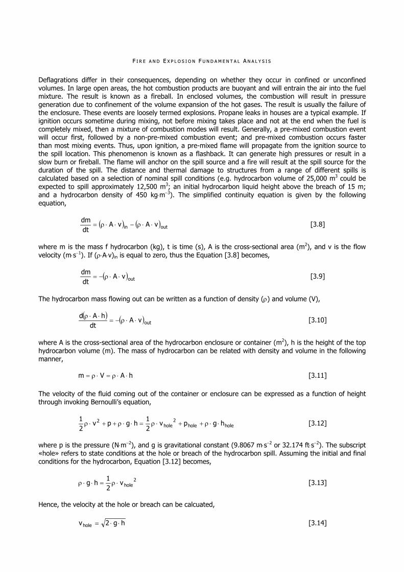
FF II RR EE AA NN DD EE XX PP LL OO SS II OO NN FF UU NN DD AA MM EE NN TT AA LL AA NN AA LL YY SS II SS
Deflagrations differ in their consequences, depending on whether they occur in confined or unconfined volumes. In large open areas, the hot combustion products are buoyant and will entrain the air into the fuel mixture. The result is known as a fireball. In enclosed volumes, the combustion will result in pressure generation due to confinement of the volume expansion of the hot gases. The result is usually the failure of the enclosure. These events are loosely termed explosions. Propane leaks in houses are a typical example. If ignition occurs sometime during mixing, not before mixing takes place and not at the end when the fuel is completely mixed, then a mixture of combustion modes will result. Generally, a pre-mixed combustion event will occur first, followed by a non-pre-mixed combustion event; and pre-mixed combustion occurs faster than most mixing events. Thus, upon ignition, a pre-mixed flame will propagate from the ignition source to the spill location. This phenomenon is known as a flashback. It can generate high pressures or result in a slow burn or fireball. The flame will anchor on the spill source and a fire will result at the spill source for the duration of the spill. The distance and thermal damage to structures from a range of different spills is calculated based on a selection of nominal spill conditions (e.g. hydrocarbon volume of 25,000 m3 could be expected to spill approximately 12,500 m3; an initial hydrocarbon liquid height above the breach of 15 m; and a hydrocarbon density of 450 kgm3). The simplified continuity equation is given by the following equation,
outin vAvAdtdm
[3.8]
where m is the mass f hydrocarbon (kg), t is time (s), A is the cross-sectional area (m2), and v is the flow velocity (ms1). If (Av)in is equal to zero, thus the Equation [3.8] becomes,
outvAdtdm
[3.9]
The hydrocarbon mass flowing out can be written as a function of density () and volume (V),
outvAdt
hAd
[3.10]
where A is the cross-sectional area of the hydrocarbon enclosure or container (m2), h is the height of the top hydrocarbon volume (m). The mass of hydrocarbon can be related with density and volume in the following manner,
hAVm [3.11] The velocity of the fluid coming out of the container or enclosure can be expressed as a function of height through invoking Bernoulli’s equation,
holehole2
hole2 hgpv
21
hgpv21
[3.12]
where p is the pressure (Nm2), and g is gravitational constant (9.8067 ms2 or 32.174 fts2). The subscript «hole» refers to state conditions at the hole or breach of the hydrocarbon spill. Assuming the initial and final conditions for the hydrocarbon, Equation [3.12] becomes,
2holev
21
hg [3.13]
Hence, the velocity at the hole or breach can be calcuated,
hg2vhole [3.14]

FF II RR EE AA NN DD EE XX PP LL OO SS II OO NN RR II SS KK AA NN AA LL YY SS II SS
Multiplying by a discharge coefficient to account for resistance of the hole,
hg2Cv dhole [3.15]
and substituting the Equation [3.15] in the Equation [3.10],
hg2CA
dthAd
dhole
[3.16]
Integrating Equation [3.16] becomes,
t
0d
h
h
dtChg2
dh
i
[3.17]
and hi is the initial height of the top hydrocarbon volume (m) when the initial time is zero (t=0). Simplifying Equation [3.18] and solving to time (t), then the height of hydrocarbon through time can be determined,
hhC1
AA
g2
t idhole
[3.18]
Total time to drain is given by thefollowing expression,
idhole
hC1
AA
g2
t [3.19]
The flow rate will be greatest at the beginning of the spill, due to the hydrostatic head having a maximum. The flow rate has a linear dependence on time, so an average flow rate can be determined by dividing the maximum flow rate by 2. The maximum flow rate can be found by substituting Equation [3.15] into Equation [3.10], and using Equation [3.11] to express in terms of volume per time. Then the average flow rate (m3s1) that leaves the hole is given by,
ihole
davg
hg22
AC
dtdV
[3.20]
The diameter (d) of the spill is determined by assuming a steady state where the mass coming in is balanced by the mass going out,
outin vAvA [3.21] due to the heat flux from the heating of the water below and from the fire above, denoted by νtotal.
total
2
avg
v4d
dtdV
[3.22]
Thus, the diameter (d) of the spill is determined by the following expression derived from Equation [3.22],

FF II RR EE AA NN DD EE XX PP LL OO SS II OO NN FF UU NN DD AA MM EE NN TT AA LL AA NN AA LL YY SS II SS
avgtotal dtdV
v4
d
[3.23]
A cylinder, solid flame model was used to model the pool fire. The effect of wind on the flame was considered negligible. The Moorehouse correlation was used to calculate flame height (Hf), found on Fire Protection Engineering Handbook (2nd edition, 1995). The term vwind is a non-dimensional wind velocity taken to be 1.0 for low wind speeds.
044.0wind
254.0
af v
dg
md2.6H
[3.24]
where a is the air density in average conditions. The radiative flux (q) incident upon an object can be determined by the following expression,
FEq [3.25] where E is an average surface emissive power (kWm2), F is the view factor, and is transmissivity. The non-dimensional distance from the flame axis as a function of view factor and fire height-to-radius ratio, can be determined if we specified the radiantive flux (q), the surface emissive power (E), and the transmissivity (); the view factor (F) can be determined by Equation [3.25], and height-to-radius ratio from Equation [3.24]. Then the thermal hazard distance can be determined from Figure 3-11.13 of Fire Protection Engineering Handbook (2nd edition, 1995) on page 3-210. Using the nominal conditions, an analysis was performed that looked at the potential ranges of spill and fire conditions available from experimental literature. Example results of this sensitivity analysis are presented in the Table 3.20.
Table 3.20 – Summary of results of the above four liquified natural gas (LNG) spill studies.
DDiissttaannccee ttoo…… HHoollee SSiizzee ((mm22))
DDiisscchhaarrggee CCooeeffffiicciieenntt
BBuurrnn RRaattee ((mm//ss))
SSuurrffaaccee EEmmiissssiivvee PPoowweerr ((kkWW//mm22))
PPooooll DDiiaammeetteerr
((mm))
BBuurrnn TTiimmee ((mmiinn)) 3377..55
kkWW//mm22 55
kkWW//mm22 AAcccciiddeennttaall EEvveennttss
1 0.6 3104 220 148 40.0 177 554 2 0.6 3104 220 209 20.0 250 784
IInntteennttiioonnaall EEvveennttss 2 0.6 3104 220 209 20.0 250 784 5 0.6 3104 220 330 8.1 391 1,305 5 0.9 220 405 5.4 478 1,579 10 0.6 3104 220 467 4.1 548 1,823
The results in Table 3.20 suggest that, for most of the credible accidental breach and spill scenarios, the general distance for major structural damage (high hazards where the thermal intensity is about 37.5 kWm2) can occur, on average, up to 250 m from a spill. The results also suggest that, for most of the credible intentional breach and spill scenarios, the general 145 distance for major structural damage (high hazards) can occur, on average, up to 500 m from a spill. In general, the distance to low thermal hazard levels, about 5 kWm2 is about 600 m to 750 m for accidental spills and approximately 1,600 m for intentional spills. For a very large, cascading spill, high hazard zones could approach 2,000 m. These results were used to help quantify the hazard zone identification and hazard level identification for various breach and spill events. MM AA SS SS FF II RR EE SS AA NN DD PP OO OO LL FF II RR EE SS All of the hydrocarbon fire studies reviewed assume that a single, coherent pool fire can be maintained for very large pool diameters, i.e greater than 100 m. This might be unlikely due to the inability of air to get into the interior of the fire and support combustion. At some very large size, the flame envelope would break up

FF II RR EE AA NN DD EE XX PP LL OO SS II OO NN RR II SS KK AA NN AA LL YY SS II SS
into multiple flamelets. The heights of these flamelets are much less than the fuel bed diameter (Zukoski, 1986, 1995; Corlett, 1994). The break up into flamelets would result in a much shorter flame height than that assumed by the reviewed studies, which are applying height correlations far out of the diameter range for which they were developed. It is expected that the height-to-pool radius diameter would probably be much smaller than that predicted by existing correlations. The correlations predict an height-to-pool diameter ratio between 1.0 and 2.0, while a more realistic ratio for a mass fire would be under 0.5. The view factor is very sensitive to flame height at distances not close to the fire, i.e. greater than 1 times the pool diameter. View factors are used to determine how much radiative flux an object receives. Thus, if a more realistic flame height is used, lower than that which is typically calculated, then the amount of heat flux that an object receives would be less, thereby decreasing the thermal hazard zone. The zone could be decreased by a factor of two to three, depending upon the damaging heat flux levels of interest. Various correlations for flame height have been developed for a range of pool diameters up to 30 m. The height-to-pool diameter ratio correlations are typically expressed in terms of a non-dimensional heat release rate (Zukoski, 1986, 1995). This study is based upon pool fire tests where fuel vaporization is not affected by a substrate (such as water); therefore, this study should not be used for the determination of when a pool breaks up into flamelets for hydrocarbon (LNG) pool fires on water. As pool diameter increases, the non-dimensional heat
release rate decreases because it is proportional to d
1. Zukoski states that there are different transition
regions that occur. For very large pool fires, the flame breaks up into a number of independent flamelets as the non-dimensional heat release rate decreases, and the flame height depends on the diameter and the heat release rate. Several researchers presented several flame height correlations with the dimensionalness burning rate (combustion Froud number) based on experimental information. The Froud number (dimensionalness burning rate) is determined by,
Dg
mF
[3.26]
where m is the mass burning rate (kgm2s1), is the hydrocarbon density (kgm3), g is the gravity acceleration constant, and D is the pool diameter (m). Moorhouse (1982) have published that the flame height has a correlation with the Froud number as given by the following expression,
254.0F2.6DL
[3.27]
On the other hand, Thomas (1965) established a fair approximation of the flame height correlation with the combustion Froud number (using China Lake tests) given by,
32
F55DL
[3.28]
For lower values of the non-dimensional heat release rate the height of the flamelets appears to become roughly independent of the source-diameter and depends only on the local heat release rate per unit area (or fuel flow per unit area). It is unknown what the limiting diameter for break up is for hydrocarbon (LNG) pool fires on water. Using an estimate of approximately 100 m, the distance to the high and lower level hazards was calculated for a range of spill conditions. The pool diameter and flame height suggested are speculative because experiments for large pool fires have yet to be performed. Many researchers have provided flame height correlations based on pool fires much smaller than those presently being considered (Heskestad, 1998). These results suggest hydrocarbon pool fires of as much as 8,900 m in diameter before breakup, based on results of laboratory testing on approximately 7 m by 7m wood fiberboards. Whether their results can be extrapolated to very large pool fires remains to be determined. Furthermore, the emissive power decreases with increasing fire size due to smoke shielding. Values significantly lower than 220 kWm2 are possible. Other phenomena, such as the occurrence of fire whirls, may increase the hazard

FF II RR EE AA NN DD EE XX PP LL OO SS II OO NN FF UU NN DD AA MM EE NN TT AA LL AA NN AA LL YY SS II SS
by generating large columnar flames with high emissive power. These structures most often form during non circular pool shapes exposed to light winds and rarely last more than a few seconds. Smoke Extinction of Radiation Transmissivity of smoke, or soot transmissivity, in a fire to thermal radiation is given by Society of Fire Profesional Engineers (SFPE, 2002), and is expressed by the following equation,
DsCsk63.0s e [3.29]
where ks is specific soot exinction area (m2kg1), Cs is soot concentration (kgm3), and D is pool diameter (m). HH YY DD RR OO CC AA RR BB OO NN DD II SS PP EE RR SS II OO NN In most of the scenarios identified, the thermal hazards from a spill are expected to manifest as a pool fire, based on the high probability that an ignition source will be available from most of the events identified. In some instances, such as an intentional spill without a breach, an immediate ignition source might not be available and the spilled hydrocarbon vapor could, therefore, disperse as a vapor cloud. For large spills, the vapor cloud could extend to as much as 1,600 m or more, depending on spill location and site atmospheric conditions. In congested or highly populated areas, an ignition source would be likely, as opposed to remote areas, in which an ignition source might be less likely. If ignited close to the spill, the thermal loading from the vapor cloud ignition might not be significantly different from a pool fire, because the ignited vapor cloud would probably burn back to the source of liquid hydrocarbon and transition into a pool fire. If the cloud is ignited at a significant distance from the spill, the thermal hazard zones can be extended significantly. The thermal radiation from the ignition of a hydrocarbon vapor cloud can be very high within the ignited cloud and, therefore, particularly hazardous to people. Experimental data and analytical estimates for hydrocarbon vapor spreading suggest that a large vapor plume could extend to large distances, depending on atmospheric conditions. Therefore, while the impact from a vapor cloud dispersion and ignition from a large spill can potentially extend beyond 1,600 meters, the area of high impact might be reduced. This suggests that hydrocarbon vapor dispersion analysis should be conducted using site-specific atmospheric conditions, location topography, and hydrocarbon operations (i.e. transport, processing, handling and storage) to adequately assess the potential areas and levels of hazards to public safety and property, and consideration of risk mitigation measures, such as development of approaches and procedures to ignite a dispersion cloud quickly if conditions exist that the cloud would impact critical areas. To assess the extent of the potential dispersion from an hydrocarbon (LNG) spill, it is commonly used the VULCAN programming code, a validated modern computational fluid dynamics (CFD) model. The VULCAN fire field model under development at Sandia National Laboratories was derived from the KAMELEON Fire model in collaboration with SINTEF and Computational Industry Technologies, AS (Norway). VULCAN was developed for liquid and gaseous hydrocarbon fuels. The model has been used for a large number of heavy hydrocarbon fuel fires. VULCAN uses a cartesian based geometry. The code runs on single or multi-processor machines. It generally parallelizes best on six processors. It runs under LINUX and UNIX operating systems. VULCAN is a validated computational fluid dynamics (CFD) fire model that uses a standard RANS formulation of the equations of motion, where the turbulence is averaged across all time scales using a k- turbulence model. A buoyant, vorticity generation sub-model of turbulence is included for turbulence length scales below the scale of the grid. VULCAN uses Magnussen’s Eddy Dissipation Concept combustion model to relate mechanistically the local fuel, oxygen, energy, and turbulence levels to consumption of species. Soot is modeled using Magnussen’s soot model to describe mechanistically the soot formation and destruction process. VULCAN uses Leckner’s model for gas band radiation. The transport of thermal radiation is calculated using the Discrete Transfer Method of Shah to solve the radiative transport equation. Either the evaporation of a liquid pool is modeled using a user-specified evaporation rate, or by allowing the code to calculate its own evaporation rate based on heat transfer into the fuel pool. VULCAN also has a rudimentary liquid spreading model based on lubrication theory. This model predicts spreading of fuel on a horizontal surface, and is capable of modeling the dripping or draining of fuel vertically (i.e. from floor to floor in a building). In order to obtain hydrocarbon dispersion distances to lower flammable limit (LFL) for accidental events, a low wind speed and highly stable atmospheric condition were chosen because this has shown to result in the greatest distances to lower flammable limit from experiment, and thus should be the most

FF II RR EE AA NN DD EE XX PP LL OO SS II OO NN RR II SS KK AA NN AA LL YY SS II SS
conservative. As noted previously elsewhere, the chances of a large vapor dispersion from either an accidental or intentional breach is rather unlikely because of the high probability that an ignition source will be available for most of the events identified. Although, the significant distances though of potential vapor dispersion, especially for a large intentional breach, suggest that hydrocarbon vapor dispersion analysis and risk mitigation measures should be carefully considered. Location-specific environmental conditions should be carefully evaluated and appropriate safety measures implemented to ensure that public health and safety, and critical facilities and infrastructures, are adequately protected. FF II RR EE BB AA LL LL SS RR EE SS UU LL TT II NN GG FF RR OO MM AA NN HH YY DD RR OO CC AA RR BB OO NN SS PP II LL LL A fireball will result from an hydrocarbon spill only if some mixing of the fuel and air occurs prior to ignition. Thus, if ignition occurs immediately upon release, no fireball will result. For a fireball to occur there must be fuel release, spread, vaporization, and ignition after significant premixing. Fireballs might result from a delayed ignition of vaporized hydrocarbon. If all these events have occurred, a fireball is the most benign form of combustion that can result. The hazards are principally short-time thermal damage high in the air and away from structures and people. The duration of the fireball from combusting clouds is given as,
2.0M6.4t [3.30] in which M is the fuel mass (in metric tons) and t is time duration of the fireballs (s). Similarly, the maximum radius (rmax) of the fireball is given as,
35.0max M23r [3.31]
in which the radius is given in meters. The thermal flux from the fireballs was also measured. Peak fluxes for combusting gasoline were in the 150 kWm2 to 330 kWm2 range. Hydrocarbons would be expected to have similar behavior. These flux levels are of the same order of magnitude as those from a pool fire. Unlike a pool fire, however, the fireball is of short duration (in the order of seconds to tens of seconds), depending upon the mass of fuel in the air. The fireball will entrain and burn all flammable vapors and provide an ignition source to the underlying liquid spill. The overall threat from a fireball is typically not of primary concern if a long duration pool fire follows it. TT HH EE RR MM AA LL DD AA MM AA GG EE OO NN SS TT RR UU CC TT UU RR EE SS The potential for damage to other vessels or structures from an hydrocarbon spill and fire needs to be considered to determine the overall risk. The potential for fire damage from spills can be relatively extensive. Hydrocarbon spills could take anywhere from 10 minutes to 20 minutes to release up to 50% of the hydrocarbon in an individual tank for a large spill and up to one hour for a small spill, depending on the location. The thermal radiation that will damage structures is approximately 37 kWm2 for durations of more than 10 minutes. Damage can be expected to the facilities and nearby steel structures, because steel strengths are reduced to about 60% or 75% of their room temperature values at 800K. Further reduction in strength will result for temperatures above 800K. Steel will melt at approximately 1,800K and is generally considered to have no strength at half the melt temperature, or 900K. The calculations suggest that these temperatures could exist at a spill from an hydrocarbon storage facility from 30 minutes to an hour and, therefore, potentially damage nearby steel and other structures. Of even greater importance is the possibility that a large spill could cause a cascading set of structural failures. In this instance, significant long-term fire damage could result to a nearby steel structure, processing plant, equipment, unloading terminal, or unloading platform. Positive operational and risk management measures can be taken to try to prevent these types of issues. Analysis of Fire Damage to Insulation Materials The insulation used in hydrocarbon operations (i.e. handling, transport, and storage) varies considerably, from rigid foams to bulk zeolite-type materials. The susceptibility of these insulation materials to either burning or thermal degradation also varies considerably. Many hydrocarbon storage facilities use foam insulation materials that include polystyrene, polyurethane, phenolic resin, and hybrid foam systems. These foams are considered combustible to slightly combustible; meaning, they will burn when exposed to an open
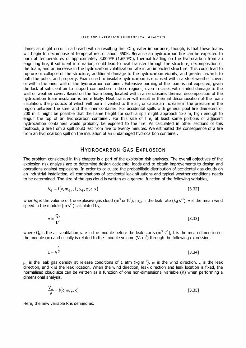
FF II RR EE AA NN DD EE XX PP LL OO SS II OO NN FF UU NN DD AA MM EE NN TT AA LL AA NN AA LL YY SS II SS
flame, as might occur in a breach with a resulting fire. Of greater importance, though, is that these foams will begin to decompose at temperatures of about 550K. Because an hydrocarbon fire can be expected to burn at temperatures of approximately 3,000ºF (1,650ºC), thermal loading on the hydrocarbon from an engulfing fire, if sufficient in duration, could lead to heat transfer through the structure, decomposition of the foam, and an increase in the hydrocarbon volatilization rate in an impacted structure. This could lead to rupture or collapse of the structure, additional damage to the hydrocarbon vicinity, and greater hazards to both the public and property. Foam used to insulate hydrocarbon is enclosed within a steel weather cover, or within the inner wall of the hydrocarbon container. Extensive burning of the foam is not expected, given the lack of sufficient air to support combustion in these regions, even in cases with limited damage to the wall or weather cover. Based on the foam being located within an enclosure, thermal decomposition of the hydrocarbon foam insulation is more likely. Heat transfer will result in thermal decomposition of the foam insulation, the products of which will burn if vented to the air, or cause an increase in the pressure in the region between the steel and the inner container. For accidental spills with general pool fire diameters of 200 m it might be possible that the flame height for such a spill might approach 150 m, high enough to engulf the top of an hydrocarbon container. For this size of fire, at least some portions of adjacent hydrocarbon containers would probably be exposed to the fire. As calculated in other sections of this textbook, a fire from a spill could last from five to twenty minutes. We estimated the consequence of a fire from an hydrocarbon spill on the insulation of an undamaged hydrocarbon container.
HH YY DD RR OO CC AA RR BB OO NN GG AA SS EE XX PP LL OO SS II OO NN The problem considered in this chapter is a part of the explosion risk analyses. The overall objectives of the explosion risk analysis are to determine design accidental loads and to obtain improvements to design and operations against explosions. In order to calculate the probabilistic distribution of accidental gas clouds on an industrial installation, all combinations of accidental leak situations and typical weather conditions needs to be determined. The size of the gas cloud is written as a general function of the following variables,
x,,,,L,m,vfV Gr,GG [3.32]
wher VG is the volume of the explosive gas cloud (m3 or ft3), mG,r is the leak rate (kgs1), v is the mean wind speed in the module (ms1) calculated by,
2a
L
Qv [3.33]
where Qa is the air ventilation rate in the module before the leak starts (m3s1), L is the mean dimension of the module (m) and usually is related to the module volume (V, m3) through the following expression,
31
VL [3.34] g is the leak gas density at release conditions of 1 atm (kgm3), is the wind direction, is the leak direction, and x is the leak location. When the wind direction, leak direction and leak location is fixed, the normalised cloud size can be written as a function of one non-dimensional variable (R) when performing a dimensional analysis,
x,,,RfVVG [3.35]
Here, the new variable R is defined as,

FF II RR EE AA NN DD EE XX PP LL OO SS II OO NN RR II SS KK AA NN AA LL YY SS II SS
v
v
Q
m
Q
QR
ref
refa
g
a
g
[3.36]
where v is the wind speed (ms1),
ref
refa
v
Q is the reference ventilation rate normalised by the reference
wind speed (when buoyancy forces are small, the ventilation rate is proportional to the wind speed), Qa is the air volume flowrate (m3s1) through the module before the leak starts, and Qg is the gas volume flowrate (m3s1). These results from the dimensional analysis suggest that the variable R should be used instead of the leakrate and the windspeed. When involved in fire and explosion, toxic fumes of carbon monoxide, nitrogen oxides and ammonia may release. These combustion related substances have the following exposure limits (Ditali et al., 2000; Faisal, 2001) listed in Table 3.21.
Table 3.21 – Exposure limit for toxic fumes.
MMaatteerriiaall OOddoorr ((ppppmm)) TTLLVV ((ppppmm)) SSTTEELL ((ppppmm)) IIDDLLHHVV ((ppppmm)) CO 50 400 1500 N2O 50 150 250 NH3 50 25 35 1000
EE XX PP LL OO SS II OO NN CC OO NN SS EE QQ UU EE NN CC EE SS AA NN AA LL YY SS II SS Fire and explosion will produce physical phenomena like blast wave, load noise, fly debris and vibration. All these will effect to the human and environment surrounding the fire and explosive area. The main factor which govern the magnitude peak overpressure in a blast wave from the detonation in free air are as following: (1) Distance of the wave from the center of explosion; (2) The weight of the charge; (3) The explosion parameters of the charge. With the assumption, it is pessimistic to express the relationship between the weight of the explosive charge (W), to the shockwaves effect at a distance (D). A common empirical formula which had been widely used to estimate the blast effect of the explosive as follow,
3333.0WZD [3.37] where Z is the scale factor for overpressure, D is the distance from the centre of explosion, W is the weight of charge in TNT equivalent (kg). The weight of charge (W) in TNT equivalent mass could be calculated by the following equation,
fCMW [3.38] where M is the weight of explosive (kg), and Cf is the conversion factor for a particular flammable or explosive material. Since Z is the scale factor for the overpressure value (P), the overpressure value can be estimated by using this formula,
3s 103.101PP [3.39]
where Ps is the scale overpressure, and P is the overpressure (N/m2). The overall risk arising from flammable and explosive material accidents, which could result in fatalities and eardrum rupture at the incident area and its surrounding area. The explosion overpressures depend on the peak overpressure that reaches the person. Direct exposure to high overpressure levels may be fatal. The fatality is a result of the direct contact

FF II RR EE AA NN DD EE XX PP LL OO SS II OO NN FF UU NN DD AA MM EE NN TT AA LL AA NN AA LL YY SS II SS
with the explosion event even though the overpressure that caused the structure collapse or damage would not directly result in a fatality if the person were in a open area. The load noise is evaluated by use the following equation,
610P1020
PLog20L [3.40]
where P is the overpressure value (N/m2). EE FF FF EE CC TT SS OO FF DD II SS PP EE RR SS II OO NN PP AA RR AA MM EE TT EE RR SS The effects of wind speed and leak rate have been combined in the non-dimensional variable (R). A constant R will give a constant cloud size as long as the velocity field in the module is created by the wind field outside the platform and not created by buoyancy effects. The reason for the similarity between two cloud sizes with equal R is that the gas concentration at any point away from the source is approximately proportional to the leakrate and inverse proportional to the wind speed. This effect has also been applied in the «frozen cloud» assumption. The values of the wind speed and leak rate are different, however, the value of R is approximately the same (R ≈0.1), for these cases the cloud size is found to be approximately the same. When R is small (i.e. small leakrate and, or large wind speed), a small cloud is obtained due to quick dilution of the cloud. For large R, the explosive cloud size is reduced because most of the gas will have concentrations higher than the Upper Explosion Limit (UEL). The cloud size reaches a maximum for an intermediate R when most of the gas and air mixture has concentration between Lower and Upper Explosion Limit (LEL and UEL). The effects of leak wind direction are in general that wind-direction opposite and equal the leak-jet direction result in large and small clouds, respectively. A larger cloud size is form due to large re-circulating zones. Large re-circulating zones are created by the large firewall. In general, the re-circulating zones results in larger gas clouds.
DD UU SS TT EE XX PP LL OO SS II OO NN Some of the most destructive explosions have been caused by dust. There is more explosive energy in the dust from grains such as wheat, barley and corn, than in an equal amount of TNT. While fires are far more common, explosions are far more costly in terms of loss of life, injury and property damage. Dust explosions have been quite common in the past. For example, there were 645 explosions in the coal mines of England from 1835 to 1850, in which coal dust was the major contributing factor. There were 1,085 dust explosions resulting in 351 fatalities, in the United States from 1900 to 1956. Also in the United States, among the 15,000 grain handling facilities from 1958 to 1977, there were 220 dust explosions resulting in 48 deaths and 500 injuries. The potential for a dust explosion has now become a well recognised hazard. What is a dust explosion? A dust explosion is the very rapid combustion of a dust cloud, to produce a flame and a pressure front. The flame front frequently causes loss of life, while the pressure front will often cause extensive damage to buildings. With some dusts, there is sometimes only a flame front and the pressure front is only minimal; with others, the flame spreads with the effect of an explosion. An explosion occurs as the flame generates heat and combustion products, and expansion from both these sources causes an immediate pressure rise which must then move out as a pressure wave and impact on the surroundings. Pressures of up to 700 kNm2 to 800 kNm2 can be generated, and if it occurs in a confined space such as a building, the effects can be devastating, since most buildings can only withstand 2 kNm2 at most. Why so dangerous? Dust explosions are dangerous, because they can set off a chain reaction. The initial explosion is usually small and localised, however it is often sufficient to disturb surrounding dust deposited on floors, roofs, beams, and machinery to form a second much larger cloud, which in turn can lead to a far more devastating explosion. Further explosions can follow in other parts of the building or even neighbouring buildings. These explosions may occur seconds or even minutes apart, and have been described by those who have survived a dust explosion, as sounding like «rolling thunder». A fire can then follow from scattered burning particles, or from other small dust accumulations that have been ignited. Dust is readily ignited and can burn fiercely or explode. Spontaneous combustion can occur, so dust should be kept under control. Environments should be regularly cleaned to avoid the risk of fire. A wise solution can prevent a loss of lives, money and downtime. Combustible particulate solids are defined as any combustible

FF II RR EE AA NN DD EE XX PP LL OO SS II OO NN RR II SS KK AA NN AA LL YY SS II SS
solid material, composed of distinct particles or pieces, regardless of size, shape, or chemical composition. Combustible dust can also be defined as a combustible particulate solid that presents a fire or deflagration hazard when suspended in air or some other oxidizing medium over a range of concentrations, regardless of particle size or shape. Why the distinction between a combustible particulate solid and combustible dust? Even though a combustible particulate solid might not ignite readily or be capable of being suspended in air in its particulate form (the pieces could be too large), the material can break down during such activities as shipping, handling, conveying, mixing, and pulverizing. It will then become an immediate hazard in its dust form if a source of ignition is available. Pneumatic conveying equipment and dust control exhaust systems that transport combustible particulate solids need to be protected from fire and dust explosions. Combustible particulate solids that have settled onto surfaces such as floors, platforms, suspended ceilings and building structural members as well as inside pipes and ducts can burn if exposed to a source of ignition. If combustible particulate solids are thrown into the workplace air during cleaning or by excessive drafts in the plant, the resulting combustible dust can present a fire or deflagration hazard if exposed to an ignition source. If the concentration of suspended combustible solids is above the Minimum Explosion Concentration (MEC) and the source of ignition produces energy above the Minimum Ignition Energy (MIE), the dust will ignite. If the combustible dust is in a confined space such as in a room, silo, bin, filter-receiver, dust collector or cyclone, the burning dust can produce enough pressure for a deflagration to occur. CC OO NN TT RR II BB UU TT II NN GG FF AA CC TT OO RR SS The initial explosion need not necessarily be caused by dust. It may only be a small gas or vapour explosion, or even a mechanical or man made disturbance sufficient to create a dust cloud. Dust clouds may be ignited by the effects of mechanical friction such as overheated bearings, motors overheating from air cooling vents being clogged with dust, particles of steel or stone caught up in grinding machinery producing sparks, overheated dust coated light bulbs, static electricity, electrical arcing, welding sparks and naked flames. As a general rule, dusts require 20 to 50 times more energy from an ignition source compared with a flammable vapour, or they need direct contact with surface temperatures ranging from 300ºC (572ºF) to 600ºC (1112ºF). The finer the dust the greater the hazard. Not only can it be more easily blown into the air, it will stay suspended in air much longer. It has a greater surface area per unit volume so that it can burn all the more rapidly, increasing the intensity of the flame front and the violence of the explosion. Dusts like flammable vapours, have lower and upper explosive limits. The lower limit is the concentration of dust in air to just sustain the flame front. The lower flammability limit ranges from about 10 gm3 (4.37 grft3) to 40 gm3 (17.48 grft3) depending on the type of dust. At these concentration it will be quite visible to the naked eye as a fog or cloud. The upper limit is usually difficult to measure since there appears to be no clear cut-off point. Instead it may, or may not, ignite at a given concentration. If it does ignite, it tends to leave behind increasing amounts of charred residue. Concentrations of dust which are potentially explosive are intolerable for people to remain in and are not likely to be found in the open, however they can be found around machinery used for crushing, grinding, sanding, milling, filtering, blending, shredding, spray drying, or conveying bulk quantities of solid materials. Additional elements needed for a combustible dust explosion are: (1) Combustible dust (fuel); (2) Ignition source (heat); (3) Oxygen in air (oxidizer). (4) Dispersion of dust particles in sufficient quantity and concentration; (5) Confinement of the dust cloud. The addition of the latter two elements to the fire triangle (Figure 3.1) creates what is known as the explosion pentagon. If a dust cloud (diffused fuel) is ignited within a confined or semiconfined vessel, area, or building, it burns very rapidly and may explode. The safety of employees is threatened by the ensuing fires, additional explosions, flying debris, and collapsing building components. An initial (primary event) explosion in processing equipment or in an area were fugitive dust has accumulated may shake loose more accumulated dust, or damage a containment system (such as a duct, vessel, or collector). As a result, if ignited, the additional dust dispersed into the air may cause one or more secondary explosions. These can be far more destructive than a primary explosion due to the increased quantity and concentration of dispersed combustible dust. If one of the elements of the explosion pentagon is missing, a catastrophic explosion can not occur. Two of the elements in the explosion pentagon are difficult to eliminate: oxygen

FF II RR EE AA NN DD EE XX PP LL OO SS II OO NN FF UU NN DD AA MM EE NN TT AA LL AA NN AA LL YY SS II SS
(within air), and confinement of the dust cloud (within processes or buildings). However, the other three elements of the pentagon can be controlled to a significant extent. HH AA ZZ AA RR DD SS AA SS SS OO CC II AA TT EE DD WW II TT HH CC OO MM BB UU SS TT II BB LL EE DD UU SS TT SS Industrial dust explosions have been a risk for as long as man has been processing, storing and transporting materials. Any combustible solid material which can be dispersed in air as a dust cloud, is capable of causing a dust explosion. Explosions on record have originated from dusts from the following sources: (1) Agriculture grain dust, flour, sugar, milk powder, wool, paper, and wood. (2) Metals aluminium, magnesium, zinc. (3) Mining coal, combustible sulphide ores. (4) Chemical industry sulphur, most plastics, pesticides, pharmaceutical's including aspirin and vitamin C. The amount of heat generated during an explosion results in extremely high pressures damaging process equipment, halting production, and placing personnel at risk of serious injury or worse. And if the explosion is allowed to propagate, subsequent explosions can occur, often with catastrophic results. Preventing the buildup of dust is one of the key means for controlling fire and explosion hazards. The principal engineering control technology for control of dust is exhaust ventilation. The primary work practice control is good housekeeping.
Ignition
Oxygen
Confinementof dust cloud
Combustibledust
Dispersion of dustparticles
Fire
Figure 3.2 – Fire, dust and explosion combination event pentagon. The Bureau of Mines (USBM) of the United States Department of the Interior (USDI) developed an arbitrary scale (see Table 3.22) based on tests using small amounts of dusts, as a guide to the degree of hazard of each type of dust.
Table 3.22 – Explosion hazard scale for dusts (USBM).
CCllaassssiiffiiccaattiioonn IIggnniittiioonn SSeennssiivviittyy EExxpplloossiioonn SSeevveerriittyy Weak < 0.2 < 0.5
Moderate 0.2 – 1.0 0.5 – 1.0 Strong 1.0 – 5.0 1.0 – 2.0 Severe > 5.0 > 2.0
There are two terms used on the scale, the ignition sensitivity (how easy to ignite), and explosion severity (how big a bang). The higher the number on each scale the greater the hazard that each dust represents (see Table 3.23).

FF II RR EE AA NN DD EE XX PP LL OO SS II OO NN RR II SS KK AA NN AA LL YY SS II SS
Table 3.23 – Explosion potential of some dusts (USBM).
TTyyppee ooff DDuusstt IIggnniittiioonn SSeennssiivviittyy
EExxpplloossiioonn SSeevveerriittyy TTyyppee ooff DDuusstt IIggnniittiioonn
SSeennssiivviittyy EExxpplloossiioonn SSeevveerriittyy
Aluminium 7.3 > 10.2 Magnesium 3.0 7.4 Aspirin 2.4 > 4.3 Milk (powdered) 1.6 0.9 Coal 2.2 1.8 Polyethylene 24.0 2.2 Coffee bean 0.1 0.1 Polystyrene 6.0 2.0 Cotton < 0.1 < 0.1 Rubber 4.6 1.6 Egg wite < 0.1 0.2 Sugar 4.0 2.4 Flour 2.1 1.8 Sulfur 20.2 1.9 Grain dust 2.8 3.3 Vitamin C 1.0 2.2
II NN CC II DD EE NN TT SS II NN VV OO LL VV II NN GG DD UU SS TT On the 15th March, 1987, in Harbin, China, an explosion of flax dust triggered a chain of explosions that destroyed the whole 13,000 m2 linen plant, causing 58 deaths and 177 injuries. The strength and time of each explosion was detected at the nearby earthquake monitoring station. On the 2nd March, 1982, in the United Kingdom, an articulated lorry carrying 19 tonnes of powdered resin crashed into a roadside cottage spilling part of its load. A dust cloud was thrown up, which ignited and exploded, setting fire to the entire load. Noxious fumes from the fire affected the driver, occupants of the cottage, workmen at the nearby building site and some fishermen in a boat about 1.5 kilometres out to sea. In the United States on 23rd December, 1977, at Westwego, Louisiana, a series of explosions destroyed 37 grain silos completely and damaged many others, causing 35 deaths and USD 100,000,000 worth of damage. The facility consisted of 73 silos with a capacity of 150,000 m3. It was one of 5 grain storage explosions that occurred over an 8 day period, and was attributed to unusually dry weather conditions. On the 6th February, 1979, in Bremen, Germany, the greater part of the 40,000 square metre Roland Mill complex was destroyed by a series of explosions. The complex included a seven story flour store, six story mill, other silos and administration building. A pressure wave struck a loaded truck, throwing it against a wall spreading its load into the air and believed to have caused an open air explosion. No traces were found of seven of the fourteen killed in the fire, believed to be cremated in parts of the fire where all traces of combustibles were consumed; an estimated 1,000 ºC for several hours. In February 1999, a deadly fire and explosion occurred in a foundry in Massachusetts (United States). The Occupational Safety Health Administration (OSHA) and state and local officials conducted a joint investigation of this incident. The joint investigation report indicated that a fire initiated in a shell molding machine from an unknown source and then extended into the ventilation system ducts by feeding on heavy deposits of phenol formaldehyde resin dust. A small primary deflagration occurred within the ductwork, dislodging dust that had settled on the exterior of the ducts. The ensuing dust cloud provided fuel for a secondary explosion which was powerful enough to lift the roof and cause wall failures. Causal factors listed in the joint investigation report included inadequacies mainly in the following area of housekeeping to control dust accumulations. In January 2003, devastating fires and explosions destroyed a North Carolina pharmaceutical plant that manufactured rubber drug-delivery components. Six employees were killed and 38 people, including two firefighters, were injured. The United States Chemical Safety and Hazard Investigation Board (CSB), an independent Federal agency charged with investigating chemical incidents, issued a final report concluding that an accumulation of a combustible polyethylene dust above the suspended ceilings fueled the explosion. The Chemical Safety and Hazard Investigation Board was unable to determine what ignited the initial fire or how the dust was dispersed to create the explosive cloud in the hidden ceiling space. The explosion severely damaged the plant and caused minor damage to nearby businesses, a home, and a school. In February 2003, a Kentucky (United States) acoustics insulation manufacturing plant was the site of another fatal dust explosion: 7 killed, 37 injured. The Chemical Safety and Hazard Investigation Board also investigated this incident. Their report cited the likely ignition scenario as a small fire extending from an unattended oven which ignited a dust cloud created by nearby line cleaning. This was followed by a deadly cascade of dust explosions throughout the plant.

FF II RR EE AA NN DD EE XX PP LL OO SS II OO NN FF UU NN DD AA MM EE NN TT AA LL AA NN AA LL YY SS II SS
Finely dispersed airborne metallic dust can also be explosive when confined in a vessel or building. In October 2003, an Indiana (United States) plant where auto wheels were machined experienced an incident: 1 killed, 1 injured. A story similar to the previously discussed organic dust incidents: aluminium dust was involved in a primary explosion near a chip melting furnace, followed by a secondary blast in dust collection equipment. In the late 1970s a series of devastating grain dust explosions in grain elevators left 59 people dead and 49 injured. In response to these catastrophic events, Occupational Safety Health Administration (OSHA) issued a “Grain Elevator Industry Hazard Alert” to provide employers, employees, and other officials with information on the safety and health hazards associated with the storage and distribution of grain. The lessons learned in the grain industry can be applied to other industries producing, generating, or using combustible dust. SS TT RR AA TT EE GG YY FF OO RR DD UU SS TT EE XX PP LL OO SS II OO NN PP RR OO TT EE CC TT II OO NN Everyone wants to assure that their plant is safe to work in. But how do you begin to evaluate the safety conditions in your plant if it is processing combustible particulate solids? A combustible dust explosion hazard may exist in a variety of industries, including food (e.g. candy, starch, flour, feed), plastics, wood, rubber, furniture, textiles, pesticides, pharmaceuticals, dyes, coal, metals (e.g. aluminium, chromium, iron, magnesium, and zinc), and fossil fuel power generation. The vast majority of natural and synthetic organic materials, as well as some metals, can form combustible dust, any industrial process that reduces a combustible material and some normally non-combustible materials to a finely divided state presents a potential for a serious fire or explosion. Facilities should carefully identify the following in order to assess their potential for dust explosions: (1) Materials that can be combustible when finely divided; (2) Processes which use, consume, or produce combustible dusts; (3) Open areas where combustible dusts may build up; (4) Hidden areas where combustible dusts may accumulate; (5) Means by which dust may be dispersed in the air; (6) Potential ignition sources. The primary factor in an assessment of these hazards is whether the dust is in fact combustible. Any material that will burn in air in a solid form can be explosive when in a finely divided form. Combustible dust is defined as any finely divided solid material that is 420 microns or smaller in diameter and presents a fire or explosion hazard when dispersed and ignited in air. Different dusts of the same chemical material will have different ignitability and explosibility characteristics, depending upon many variables such as particle size, shape, and moisture content. Additionally, these variables can change while the material is passing through process equipment. For this reason, published tables of dust explosibility data may be of limited practical value. In some cases, dusts will be combustible even if the particle size is larger than that specified in the definition, especially if the material is fibrous. Dust collection is best accomplished at the source at the point of operation of the equipment, if feasible. For many pieces of equipment, well-designed ducts and vacuum hoods can collect most of the dust generated before it even reaches the operator. Very fine dust that manages to escape point-of-source collection can be captured from above by general exhaust points located along the ceiling. These control technologies are effective for most equipment, excepting machines that commonly produce the very finest dust or large quantities of dust. The amount of dust accumulation necessary to cause an explosive concentration can vary greatly. This is because there are so many variables like the particle size of the dust, the method of dispersion, ventilation system modes, air currents, physical barriers, and the volume of the area in which the dust cloud exists or may exist. As a result, simple rules of thumb regarding accumulation (such as writing in the dust or visibility in a dust cloud) can be subjective and misleading. The hazard analysis should be tailored to the specific circumstances in each facility and the full range of variables affecting the hazard. Many locations need to be considered in an assessment. One obvious place for a dust explosion to initiate is where dust is concentrated. In equipment such as dust collectors, a combustible mixture could be present whenever the equipment is operating. Other locations to consider are those where dust can settle, both in occupied areas and in hidden concealed spaces. A thorough analysis will consider all possible scenarios in which dust can be disbursed, both in the normal process and potential failure modes. The following are some recommendations for the control of dusts to prevent explosions:
FF II RR EE AA NN DD EE XX PP LL OO SS II OO NN RR II SS KK AA NN AA LL YY SS II SS
(1) Minimize the escape of dust from process equipment or ventilation systems; (2) Use dust collection systems and filters; (3) Utilize surfaces that minimize dust accumulation and facilitate cleaning; (4) Provide access to all hidden areas to permit inspection; (5) Inspect for dust residues in open and hidden areas, at regular intervals; (6) Clean dust residues at regular intervals; (7) Use cleaning methods that do not generate dust clouds, if ignition sources are present; (8) Only use vacuum cleaners approved for dust collection; (9) Locate relief valves away from dust hazard areas; (10) Develop and implement a hazardous dust inspection, testing, housekeeping, and control program
(preferably in writing with established frequency and methods). Good housekeeping extends to periodic hand cleaning of your entire facility, as some dust will escape from even the best exhaust system and will eventually accumulate on rafters and other out-of-the- way spots. Also, it is extremely important to inspect and clean your exhaust ventilation system on a regular basis to maintain maximum efficiency.
(11) Regular cleaning frequencies shall be established for floors and horizontal surfaces, such as ducts, pipes, hoods, ledges and beams to minimize dust accumulations within occupied and unoccupied areas of the facility. Surfaces shall be cleaned in a manner that minimizes the generation of dust clouds.
Safe housekeeping methods to clean combustible dust that has settled onto the various surfaces in the
plant. Dust layers 321
inch (0.794 mm) thick can be sufficient to require immediate cleaning of the area.
Workers are the first line of defence in preventing and mitigating fires and explosions. If the people closest to the source of the hazard are trained to recognize and prevent hazards associated with combustible dust in the plant, they can be instrumental in recognizing unsafe conditions, taking preventative action, and alerting management. While standards require training for certain employees, all employees should be trained in safe work practices applicable to their job tasks, as well as on the overall plant programs for dust control and ignition source control. They should be trained before they start work, periodically to refresh their knowledge, when reassigned, and when hazards or processes change. A qualified team of managers should be responsible for conducting a facility analysis (or for having one done by qualified outside persons) prior to the introduction of a hazard and for developing a prevention and protection scheme tailored to their operation. Supervisors and managers should be aware of and support the plant dust and ignition control programs. Their training should include identifying how they can encourage the reporting of unsafe practices and facilitate abatement actions. Inspection and maintenance have various benefits. These benefits can include: (1) Less process downtime. (2) Geater plant morale and productivity. (3) Reduced maintenance costs. (4) More effective dust control for a healthier environment and improved product quality. (5) Good public relations.
BB II BB LL II OO GG RR AA PP HH YY Amyotte, P., Kahn, F., and Dastidar, A., Reduce dust explosions the inherently safer way, Chemical Engineering Progress, vol. 99, No. 10, October 2003, pp. 36-43. Anderson, R. P., and Armstrong, D. R., 1972. Experimental study of vapor explosions, 3rd International conference on liquefied natural gas, Washington, DC. Bartknecht, W., Dust explosions: Course, prevention, and protection, Springer Verlag, 1989. Beard, R., 1982. Inorganic compounds of oxygen, nitrogen, and carbon, in Patty’s Industrial Hygiene and Toxicology, Volume 2C – Toxicology, George D. Clayton and Florence E Clayton, editors, Wiley Interscience, New York. Berthoud, G., 2000. Vapor explosions, Annu. Rev. Fluid Mech., 32, 673-611. Blevins, R. D., 1984. Applied fluid dynamics handbook, Van Nostrand Reinhold Company, Inc., pp. 136-141. Boe, R., 1998. Pool boiling of hydrocarbon mixtures on water, Int. J. Heat Mass Transfer, Vol. 41, No. 8-9, 1003-1011.

FF II RR EE AA NN DD EE XX PP LL OO SS II OO NN FF UU NN DD AA MM EE NN TT AA LL AA NN AA LL YY SS II SS
Bowen, J. E., An overview: Grain dust explosions. Fire Engineering, 136(1983):22,23,25,27. Britton, L.G., Cashdollar, K.L, Fenlon, W., Frurip, D., Going, J., Harrison, B.K., Niemeier, J., and Ural, E.A., The role of ASTM E27 methods in hazard assessment (Part II): Flammability and ignitability, Process Safety Progress, vol. 24, pp. 12-28, 2005. Brown, L. E. et al., 1974. Predict LNG fire radiation, Hydrocarbon Processing, 141-143. C. A. Selby and B. A. Burgan, 1998. Blast and fire engineering for topside structures (Phase II), The Steel Construction Institute Publication No. 253. Carpenter, R.A, L.J. Habegger and C.P.B. Claudio, 1990. Environmental risk assessment guidelines, Asian Development Bank. Cashdollar, K.L., Overview of dust explosibility characteristics, Journal of Loss Prevention in the Process Industries, vol. 13, pp. 183-199, 2000. Center for Chemical Process Safety (CCPS). Guidelines for safe handling of powders and bulk solids. CCPS, American Institute for Chemical Process Safety, New York, New York, January 2005. Chan, et al., 1983. Influence of confinement on flame acceleration due to repeated obstacles, Comb. Flame, 49, 27-39. Chan, S. T., December 1994. FEM3C: An Improved three-dimensional heavy-gas dispersion model: User’s manual, UCRL-MA-116567, Rev. 1, Lawrence Livermore National Laboratory. Chemical Industries Association, 1992. A guide to hazard and operability studies. Chemical Safety and Hazard Investigation Board (CSB). CSB investigators find likely source of dust explosion at indiana automotive plant. CSB News Release, Washington, DC, November 5, 2003. Chemical Safety and Hazard Investigation Board (CSB). Investigation report: West Pharmaceutical Services, Inc. dust explosion. CSB, Washington, DC, September 2004. Chemical Safety and Hazard Investigation Board (CSB). Investigation report: CTA Acoustics, Inc. combustible dust fire and explosions. CSB, Washington, DC, September 2004. Code of Federal Regulations (CFR), Standards. Congress of the United States Office of Technology Assessment, Transportation of liquefied natural gas, September 1977. Corlett, R. C., 1974. Velocity distribution in fires, in Heat Transfer in Fires, ed. P.L. Blackshear, pp. 239-255, John Wiley and Sons, New York. CPR-16E, Methods for the determination of possible damage to people ad objects resulting from releases of hazardous materials, First Edition, published by TNO, 1992. Cross, J., and Farrer, D., Dust explosions, New York: Plenum Press, 1982. D. J. Finney. Probit Analysis. Cambridge University Press, 1977. Daish, N.C., 2000. SMEDIS: Scientific model evaluation of dense gas dispersion models, Int. J. Env. and Pollution, Vol. 14, No. 1-6, 39-51. Daniel, A.C., Joseph and F. Louvar, 2001. Chemical process safety: Fundamental with applications. 2nd Ed. Prentice Hall, pp 306-312. Delichatsios, M. A., Air entrainment into buoyant jet diffusion flames and pool fires, Combustion and Flame, Volume 70, Pages 33-46, 1987. Ditali, S., M. Colombi, G. Meroschini and S. Senni, 2000. Consequence analysis in LPG installation using an intergrated computer package. J. Hazard. Mater., 71, 159-177. Ebidat, Vahid., Is your dust collection system an explosion hazard?, Chemical Engineering Progress, vol. 99, No. 10, October 2003, pp. 44-49. Eckhoff, Rolf K., Dust explosions in the process industries, 3rd Edition, Gulf Professional Publishing, 2003. Ermak, D.L., 1980. User’s manual for SLAB: An atmospheric dispersion model for denser-than-air releases, ACRL-MA-105607, Lawrence Livermore National Laboratory. Faisal, I. Khan, S.A. 2001. Abbasi. Estimation of probabilities and likely consequences of a chain of accidents (domino effect) in Manali Industrial Complex. J. Cleaner Production, 9, 493-508. Fay, J.A., 2003. Model of spills and fires from LNG and oil tankers, Journal of Hazardous Materials, B96-2003, 171-188, 2003. Finney, D.J., 1971. Probit analysis. Cambridge University Press. Fire Protection Handbook, Ed., McKinnon, G. P., 14th ed., 1976, NFPA, Boston, Massachusets. Fletcher, D.F., and Theofanous, T.G., 1994. Recent progress in the understanding of steam explosions, J. Loss Prev. Process Ind., Vol. 7, no. 6, 457-462.

FF II RR EE AA NN DD EE XX PP LL OO SS II OO NN RR II SS KK AA NN AA LL YY SS II SS
FM Global, Prevention and mitigation of combustible dust explosions and fire, Data Sheet No. 7-76, January 2005. Frank, Walter, Dust explosion prevention and the critical importance of housekeeping, Process Safety Progress, vol. 23, No. 3, September 2004, pp. 175-184. G. A. Melhem, A. S. Kalelkar, H. Ozog, and S. Saraf, Managing liquified natural gas risks: Separating the facts from the myths, IoMosaic Corporation Whitepaper, 2006. G. Opschoor, R. O. M. Van Loo, and H. J. Pasman. Methods for calculation of damage resulting from physical effects of the accidental release of dangerous materials. In International conference on hazard identification and risk analysis, human factors and human reliability in process safety, pages 21–32. Center for Chemical Process Safety, AIChE, 1992. Guidelines for Chemical Process Quantitative Risk Analysis, 2nd Edition, American Institute of Chemical Engineers Center for Chemical Process Safety (CCPS), 2000. Hankin, R. K.S., 2003. Heavy gas dispersion: Integral models and shallow layer models, J. Haz. Mat., A102, 1-10. Hatwig, M., and Steen, H. (eds.), Handbook of explosion prevention and protection, Wiley VCH, 2004. Heskestad, 1998. Dynamics of the fire plume, Phil. Trans. R. Soc. Lond. A, 356, 2815-2833. J. Wiklund and I. Fossan, 1999. Model for explosion risk quantification, Proceedings from 8th annual conference on offshore installations Fire and Explosion Engineering. Johnson, A. D., 1992. A model for predicting thermal radiation hazards from large-scale lng pool fires. Major Hazards Onshore and Offshore, Institute of Chemical Engineers, Symposium Series No. 130, EFCE Event No. 470, EFCE Publication No. 93, Manchester, October 20-22, pp: 507-524. K. Cassidy and M. F. Pantony, Major industrial risks: A technical and predictive basis for on and off site emergency planning in the context of United Kingdom legislation, Symposium Series No. 110, pages 75-95, Institute of Chemical Engineers, Hemisphere Publishing Corporation, 1988. Lee, J. H. S., and Moen I. O., 1980. The mechanism of transition from deflagration to detonation in vapor cloud explosions, Prog. Energy Combust. Sci., Vol. 6, 359-389. McGraw Hill Encyclopedia of Science of Technology, 1987. New York, McGraw Hill, pp 521-528. Mizner, G. A., and Eyre, J. A., 1983. Radiation from liquefied gas fires on water, Combustion Science and Technology, Volume 35, pp. 33-57. National Fire Protection Association (NFPA). Industrial fire hazards handbook, 3rd Edition. NFPA, Inc., Quincy, MA, 1990. National Materials Advisory Board (NMAB) Publications. Nelson, P., Dust explosions: The forgotten killer. Australian Safety News, 65(1994):51-55. O. Talberg, O. R. Hansen and J. R. Bakke, 1999. Explosion risk analysis using flacs, Proceedings from 8th annual conference on offshore installations Fire and Explosion Engineering. Occupational Safety and Health Administration (OSHA), the Massachusetts Office of the State Fire Marshall, and the Springfield Arson and Bomb Squad. Joint foundry explosion investigation team report. OSHA, Springfield, MA, (No date). Occupational Safety Health Administration (OSHA) Standards, Interpretations, and Publications. Parnarouskis, M.C. et al., 1980. Vapor cloud explosion study. Six. Congr. Int. Gaz. Natl. Liq., v. 2, Sess 3, paper 12. Porteous, W.M., and Blander, M., 1975. Limits of superheat and explosive boiling of light hydrocarbons, halocarbons and hydrocarbon mixtures, AIChE Journal, 1975, 31(3), 560-566. Pritchard, M. J., and T. M. Binding, 1992. FIRE2: A new approach for predicting thermal radiation levels from hydrocarbon pool fires, IChemE Symposium Series, No. 130, pp. 491-505. R. P. Claever, S. Burgess, G. Y. Buss, C. Savvides, S. Connolly, R. E. Ritter, 1999. Analysis of gas build-up from high pressure natural gas releases in naturally ventilated offshore modules, Proceedings from 8th annual conference on offshore installations Fire and Explosion Engineering. Tieszen, 1991. Gaseous hydrocarbon-air detonations, Combustion and Flames, Vol 84, pp 376-390, 1991. United States Chemical Safety and Hazard Investigation Board. Vander Molen, R., Nicholls, J. A., 1979. Blast wave initiation energy for detonation of methane-ethane-air mixture, Comb. Sci. Tech., Vol. 21, 75-78. Zukoski, E. E., 1986. Fire safety science, Proc. First Int. Sym., pp 7. Zukoski, E. E., 1995. Properties of fire plumes, in Combustion Fundamentals of Fire (ed. G. Cox), pp. 101-219. Academic Press, London.

FF II RR EE AA NN DD EE XX PP LL OO SS II OO NN FF UU NN DD AA MM EE NN TT AA LL AA NN AA LL YY SS II SS
SS ee cc tt ii oo nn 44
TTHHEERRMMAALL RRAADDIIAATT IIOONN MMOODDEELL
II NN TT RR OO DD UU CC TT II OO NN Industrial fires can be intense emitters of heat, smoke, and other combustion products. This is particularly true if the fuel is a hydrocarbon or petroleum based substance, with a high heat of combustion and sooting potential. The radiant energy flux can be sufficiently high to threaten both the structural integrity of neighboring facilities and buildings, and the physical safety of plant personnel, and potentially people beyond the boundaries of the facility. The United States Department of Housing and Urban Development (HUD) has established thermal radiation flux levels of 31.5 kWm2 (10,000 Btuh1ft2) for faclities and buildings and 1.4 kWm2 (450 Btuh1ft2) for people as guides in determining an «Acceptable Separation Distance» (ASD) between a fire consuming combustible liquids or gases and nearby structures and people (24 CFR Part 51, Subpart C, paragraph 51.203). The calculation procedure for determining acceptable separation distance is set forth in a publication of 1982 from the United States Department of Housing and Urban Development Guidebook entitled “Urban development siting with respect to hazardous commercial and industrial facilities”. In the quarter century since that report was released, the field of fire science has grown rapidly, leading to improved methods of measurement and prediction of fire behavior. A review by the Building and Fire Research Laboratory at the National Institute of Standards and Technology (NIST) of the United States Department of Housing and Urban Development guidelines (1975) for thermal radiation flux has revealed that for certain fire scenarios the methodology can produce estimates of radiation flux that are up to an order of magnitude larger than those actually measured in field experiments. The source of this discrepancy is the assumption that the fire is unobscured by smoke, that is, a person watching the fire from a distance sees the entire extent of the combustion region. In reality, large fires of most combustible liquids and gases generate an appreciable amount of smoke.
Fire Pool
Flame Height
LuminousBand
Smoke Cloud(obscured flames)
LuminousBand
Figure 4.1 – A schematic diagram of a large liquid hydrocarbon fire.

FF II RR EE AA NN DD EE XX PP LL OO SS II OO NN RR II SS KK AA NN AA LL YY SS II SS
Depending on the fuel and the size of the fire, up to 20% of the fuel mass is converted to smoke particulate in the combustion process (Society of Fire Protection Engineers, 1999). This smoke shields much of the luminous flame region from the viewer, and it is this luminous flame region that is the source of most of the thermal radiation. This shielding effect is most pronounced for fires that are tens or hundreds of meters in diameter because of the decreased efficiency of combustion at these scales. A schematic diagram is shown in Figure 4.1. The methodology to be described in the present chapter is not dramatically different from those in the SFPE Engineering Guide. However, in order to maintain the simplicity of the original model methodology, it has been necessary to adopt a slightly different approach that emphasizes global energy conservation as a way of minimizing errors in radiation flux predictions due to uncertainties in the measurements upon which the flux calculations are based. Hence, part of the goal in this fire engineering risk analysis textbook is to produce a methodology for estimating the thermal radiation flux from fires burning either combustible liquids or gases. A partial listing of these combustible liquids and gases is given in Appendix I to Subpart C of 24 CFR Part 51, siting of Department of Housing and Urban Development – Assisted Projects Near Hazardous Operations Handling Conventional Fuels or Chemicals of an Explosive or Flammable Nature. A partial listing of hazardous liquids includes crude oil, diesel fuel, gasoline, jet fuel, kerosene and toluene. A partial listing of hazardous gases includes butane, hydrogen, liquified natural gas (LNG), liquified petroleum gas (LPG) and propane. The analysis of hazardous liquid fires is relatively independent of the type of liquid; burning rates and heat release rates do not vary significantly from fuel to fuel, nor does the nature of the fire. However, hazardous gases stored under pressure, especially liquified natural gas (LNG) and liquified petroleum gas (LPG), are not as predictable. There are a number of references to fires involving hydrocarbons fuels in which a cloud of combustible gas ignited to form fireballs on the order of 100 m in diameter. The radiation from fires fueled by gases leaking from storage tanks can cause a Boiling Liquid Expanding Vapor Explosion (BLEVE) within a tank or reservoir that not only produces a tremendous amount of thermal radiation, but also often causes parts of the tank or reservoir to be thrown tens or hundreds of meters. In particular, liquified petroleum gas (LPG) is so volatile that it is more likely to vaporize than form a liquid pool, thus much of the research into large liquid fuel fires may not be applicable to liquified petroleum gas fires.
Fire Pool
Smoke Cloud(obscured flames)
LuminousBand
Figure 4.2 – A schematic diagram for solid flame radiation model. Predicting the thermal radiative flux from a fire of leaking combustible gases is more complicated than that of a liquid fuel fire because there are a number of potential fire scenarios to consider. With a liquid fuel fire, the dynamics of the fire is more understood and predictable than with a gaseous fuel. Rather than develop a separate methodology for estimating thermal radiation for each potential gaseous fire scenario, it is preferable to employ a simple procedure which encompasses a wide variety of scenarios, removes most of the geometrical parameters from the calculation, and remains conservative. Such a method is known as the
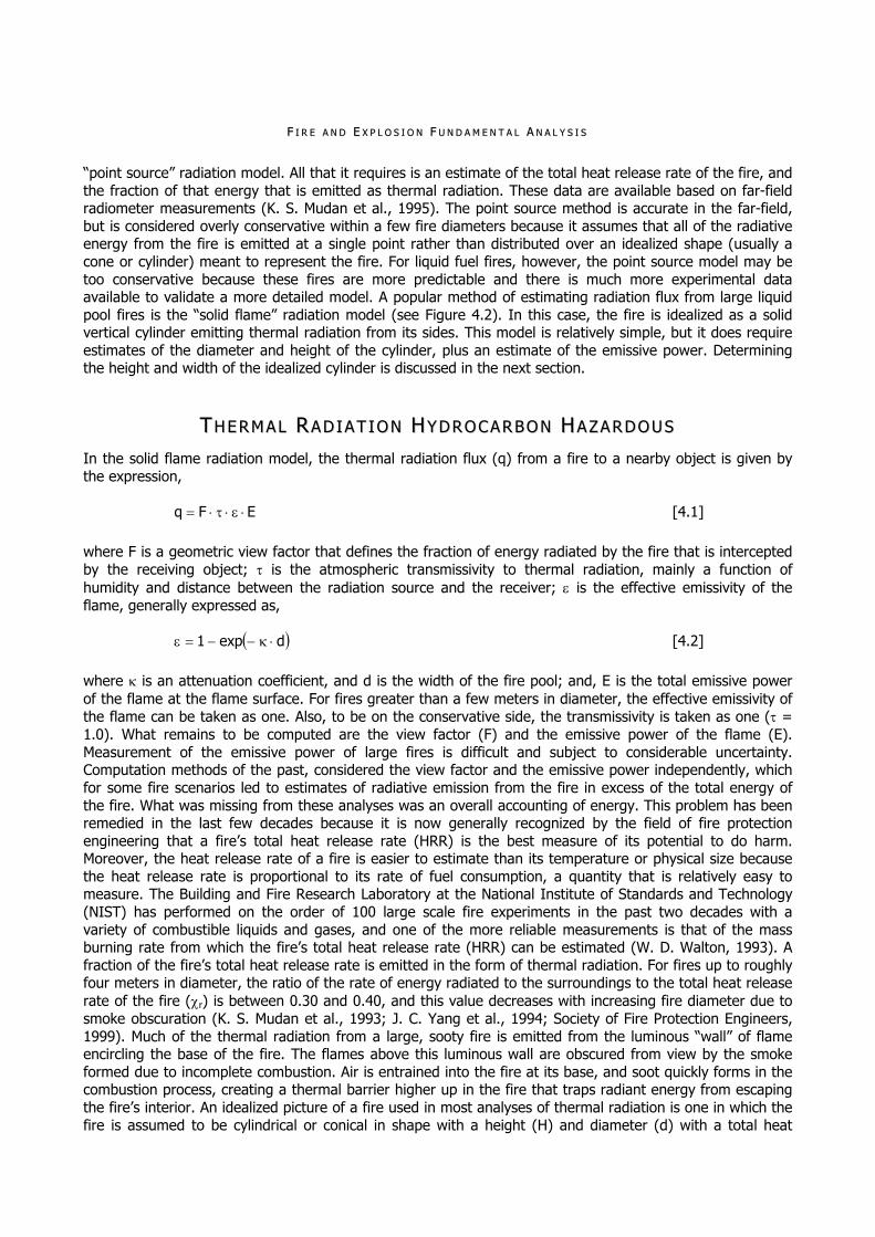
FF II RR EE AA NN DD EE XX PP LL OO SS II OO NN FF UU NN DD AA MM EE NN TT AA LL AA NN AA LL YY SS II SS
“point source” radiation model. All that it requires is an estimate of the total heat release rate of the fire, and the fraction of that energy that is emitted as thermal radiation. These data are available based on far-field radiometer measurements (K. S. Mudan et al., 1995). The point source method is accurate in the far-field, but is considered overly conservative within a few fire diameters because it assumes that all of the radiative energy from the fire is emitted at a single point rather than distributed over an idealized shape (usually a cone or cylinder) meant to represent the fire. For liquid fuel fires, however, the point source model may be too conservative because these fires are more predictable and there is much more experimental data available to validate a more detailed model. A popular method of estimating radiation flux from large liquid pool fires is the “solid flame” radiation model (see Figure 4.2). In this case, the fire is idealized as a solid vertical cylinder emitting thermal radiation from its sides. This model is relatively simple, but it does require estimates of the diameter and height of the cylinder, plus an estimate of the emissive power. Determining the height and width of the idealized cylinder is discussed in the next section.
TT HH EE RR MM AA LL RR AA DD II AA TT II OO NN HH YY DD RR OO CC AA RR BB OO NN HH AA ZZ AA RR DD OO UU SS In the solid flame radiation model, the thermal radiation flux (q) from a fire to a nearby object is given by the expression,
EFq [4.1] where F is a geometric view factor that defines the fraction of energy radiated by the fire that is intercepted by the receiving object; is the atmospheric transmissivity to thermal radiation, mainly a function of humidity and distance between the radiation source and the receiver; is the effective emissivity of the flame, generally expressed as,
dexp1 [4.2] where is an attenuation coefficient, and d is the width of the fire pool; and, E is the total emissive power of the flame at the flame surface. For fires greater than a few meters in diameter, the effective emissivity of the flame can be taken as one. Also, to be on the conservative side, the transmissivity is taken as one ( = 1.0). What remains to be computed are the view factor (F) and the emissive power of the flame (E). Measurement of the emissive power of large fires is difficult and subject to considerable uncertainty. Computation methods of the past, considered the view factor and the emissive power independently, which for some fire scenarios led to estimates of radiative emission from the fire in excess of the total energy of the fire. What was missing from these analyses was an overall accounting of energy. This problem has been remedied in the last few decades because it is now generally recognized by the field of fire protection engineering that a fire’s total heat release rate (HRR) is the best measure of its potential to do harm. Moreover, the heat release rate of a fire is easier to estimate than its temperature or physical size because the heat release rate is proportional to its rate of fuel consumption, a quantity that is relatively easy to measure. The Building and Fire Research Laboratory at the National Institute of Standards and Technology (NIST) has performed on the order of 100 large scale fire experiments in the past two decades with a variety of combustible liquids and gases, and one of the more reliable measurements is that of the mass burning rate from which the fire’s total heat release rate (HRR) can be estimated (W. D. Walton, 1993). A fraction of the fire’s total heat release rate is emitted in the form of thermal radiation. For fires up to roughly four meters in diameter, the ratio of the rate of energy radiated to the surroundings to the total heat release rate of the fire (r) is between 0.30 and 0.40, and this value decreases with increasing fire diameter due to smoke obscuration (K. S. Mudan et al., 1993; J. C. Yang et al., 1994; Society of Fire Protection Engineers, 1999). Much of the thermal radiation from a large, sooty fire is emitted from the luminous “wall” of flame encircling the base of the fire. The flames above this luminous wall are obscured from view by the smoke formed due to incomplete combustion. Air is entrained into the fire at its base, and soot quickly forms in the combustion process, creating a thermal barrier higher up in the fire that traps radiant energy from escaping the fire’s interior. An idealized picture of a fire used in most analyses of thermal radiation is one in which the fire is assumed to be cylindrical or conical in shape with a height (H) and diameter (d) with a total heat
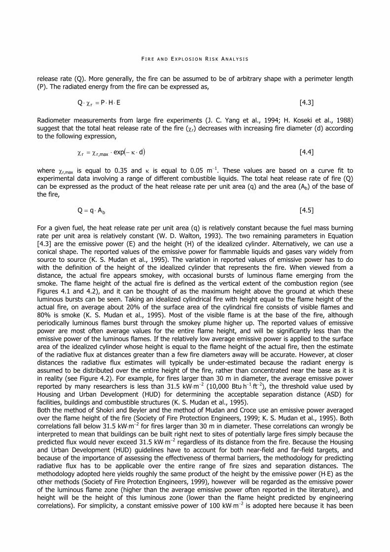
FF II RR EE AA NN DD EE XX PP LL OO SS II OO NN RR II SS KK AA NN AA LL YY SS II SS
release rate (Q). More generally, the fire can be assumed to be of arbitrary shape with a perimeter length (P). The radiated energy from the fire can be expressed as,
EHPQ r [4.3] Radiometer measurements from large fire experiments (J. C. Yang et al., 1994; H. Koseki et al., 1988) suggest that the total heat release rate of the fire (r) decreases with increasing fire diameter (d) according to the following expression,
dexpmax,rr [4.4]
where r,max is equal to 0.35 and is equal to 0.05 m1. These values are based on a curve fit to experimental data involving a range of different combustible liquids. The total heat release rate of fire (Q) can be expressed as the product of the heat release rate per unit area (q) and the area (Ab) of the base of the fire,
bAqQ [4.5] For a given fuel, the heat release rate per unit area (q) is relatively constant because the fuel mass burning rate per unit area is relatively constant (W. D. Walton, 1993). The two remaining parameters in Equation [4.3] are the emissive power (E) and the height (H) of the idealized cylinder. Alternatively, we can use a conical shape. The reported values of the emissive power for flammable liquids and gases vary widely from source to source (K. S. Mudan et al., 1995). The variation in reported values of emissive power has to do with the definition of the height of the idealized cylinder that represents the fire. When viewed from a distance, the actual fire appears smokey, with occasional bursts of luminous flame emerging from the smoke. The flame height of the actual fire is defined as the vertical extent of the combustion region (see Figures 4.1 and 4.2), and it can be thought of as the maximum height above the ground at which these luminous bursts can be seen. Taking an idealized cylindrical fire with height equal to the flame height of the actual fire, on average about 20% of the surface area of the cylindrical fire consists of visible flames and 80% is smoke (K. S. Mudan et al., 1995). Most of the visible flame is at the base of the fire, although periodically luminous flames burst through the smokey plume higher up. The reported values of emissive power are most often average values for the entire flame height, and will be significantly less than the emissive power of the luminous flames. If the relatively low average emissive power is applied to the surface area of the idealized cylinder whose height is equal to the flame height of the actual fire, then the estimate of the radiative flux at distances greater than a few fire diameters away will be accurate. However, at closer distances the radiative flux estimates will typically be under-estimated because the radiant energy is assumed to be distributed over the entire height of the fire, rather than concentrated near the base as it is in reality (see Figure 4.2). For example, for fires larger than 30 m in diameter, the average emissive power reported by many researchers is less than 31.5 kWm2 (10,000 Btuh1ft2), the threshold value used by Housing and Urban Development (HUD) for determining the acceptable separation distance (ASD) for facilities, buildings and combustible structures (K. S. Mudan et al., 1995). Both the method of Shokri and Beyler and the method of Mudan and Croce use an emissive power averaged over the flame height of the fire (Society of Fire Protection Engineers, 1999; K. S. Mudan et al., 1995). Both correlations fall below 31.5 kWm2 for fires larger than 30 m in diameter. These correlations can wrongly be interpreted to mean that buildings can be built right next to sites of potentially large fires simply because the predicted flux would never exceed 31.5 kWm2 regardless of its distance from the fire. Because the Housing and Urban Development (HUD) guidelines have to account for both near-field and far-field targets, and because of the importance of assessing the effectiveness of thermal barriers, the methodology for predicting radiative flux has to be applicable over the entire range of fire sizes and separation distances. The methodology adopted here yields roughly the same product of the height by the emissive power (HE) as the other methods (Society of Fire Protection Engineers, 1999), however will be regarded as the emissive power of the luminous flame zone (higher than the average emissive power often reported in the literature), and height will be the height of this luminous zone (lower than the flame height predicted by engineering correlations). For simplicity, a constant emissive power of 100 kWm2 is adopted here because it has been

FF II RR EE AA NN DD EE XX PP LL OO SS II OO NN FF UU NN DD AA MM EE NN TT AA LL AA NN AA LL YY SS II SS
cited as the emissive power of the luminous spots in gasoline and kerosene fires (K. S. Mudan et al., 1995). The height of the luminous flame zone (HLZ) can be found from Equation [4.3]. To simplify the analysis, the fire area is assumed circular,
dP [4.6] Hence, total heat release rate of fire is given by,
q2d
Q2
[4.7]
but this is not a restrictive assumption. Substituting expressions for the total heat release rate of the fire (r) and the total heat release rate of fire (Q) into Equation [4.3] yields an expression for the height (H),
dexpEq
4d
H max,r
[4.8]
The height (H) is plotted as a function of the diameter (d). Because of the scarcity of data about the total heat release rate of the fire (r) and the total heat release rate of fire (Q) for very large fires, it is assumed that for fires with diameters greater than 20 m, the height of the luminous flame zone remains at its maximum value. The maximum value of the height (H) is found by substituting the diameter (d) by 20 m, the total heat release rate of the fire (r) by 0.35, the attenuation coefficient () by 0.05 m1, and the total emissive power of the flame at the flame surface (E) by 100 kWm2 into Equation [4.8]. What remains of calculating the thermal radiation flux using Equation [4.1] is determining the view factor (F) from the fire to a target. The view factor calculation can be simplified by assuming the fire is surrounded by a vertical wall of height (H) emitting radiation energy (E) at a constant rate, and that the wall is composed of circular or linear elements for which analytical recipes of the view factor are available. The presence of man-made or natural thermal barriers can be incorporated into the view factor calculation. Although the methodology presented in this text is designed to be conservative, it is not conservative in one regard. Because the radiative energy output is concentrated near the base of the fire rather than distributed over the entire height of the fire, the effectiveness of a thermal barrier in blocking thermal radiation might be exaggerated. Recent measurements in Japan (N. Takahashi et al., 1999) of a 20 m diameter crude oil fire showed that 85% of the radiant energy of the fire was emitted at heights lower than 20 m. The remaining 15% of the radiant energy was emitted mainly by hot black smoke at higher levels, and by occasional luminous bursts of flame. The total heat release rate (HRR) per unit area, for crude oil is approximately 2,000 kWm2, thus according to Equation [4.8], the luminous flame height for a 20 m diameter pool fire is between 12.5 m and 13 m. In this context, a thermal barrier 13 m in height would be expected to block all of the thermal radiation. To remedy the situation, it is suggested that for the purpose of evaluating a thermal barrier, the emissive power of the flame be reduced by a half, from 100 kWm2 down to 50 kWm2. Energy conservation will be preserved by noting that the height of the luminous zone will double as a result of the lower estimate of the emissive power. The quantity HE remains the same, thus the prediction of radiative flux in the far-field remains the same. The range of emissive powers between 50 kWm2 and 100 kWm2 is not arbitrary. Many researchers have made emissive power measurements of large pool fires that fall in this range as seen previously in this textbook. It is a difficult measurement to make because in reality the emissive power is both spatially and temporally varying. The choices of 100 kWm2 for near-field hazard calculations and 50 kWm2 for the evaluation of thermal barriers are intended to yield conservative estimates of acceptable separation distance (ASD). Fire scenarios involving combustible gases vary widely, from a pool fire of a liquified gas, like liquified natural gas (LNG) or liquified petroleum gas (LPG), to a flare formed by burning vapors escaping a storage tank, to a fireball following the release of a large amount of gas that subsequently ignites. Because it is difficult to predict the structure of the fire, it is important to employ a methodology for predicting the thermal radiation flux from the fire. The simplest method of calculating the thermal radiation, known as the “point source” model, is to estimate the heat release rate of the fire, assume a fraction of the total energy is released in the
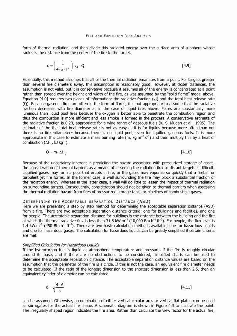
FF II RR EE AA NN DD EE XX PP LL OO SS II OO NN RR II SS KK AA NN AA LL YY SS II SS
form of thermal radiation, and then divide this radiated energy over the surface area of a sphere whose radius is the distance from the center of the fire to the target.
Qr4
1q r2
[4.9]
Essentially, this method assumes that all of the thermal radiation emanates from a point. For targets greater than several fire diameters away, this assumption is reasonably good. However, at closer distances, the assumption is not valid, but it is conservative because it assumes all of the energy is concentrated at a point rather than spread over the height and width of the fire, as was assumed by the “solid flame” model above. Equation [4.9] requires two pieces of information: the radiative fraction (r) and the total heat release rate (Q). Because gaseous fires are often in the form of flares, it is not appropriate to assume that the radiative fraction decreases with fire diameter as in the case of liquid fires above. Flares are substantially more luminous than liquid pool fires because the oxygen is better able to penetrate the combustion region and thus the combustion is more efficient and less smoke is formed in the process. A conservative estimate of the radiative fraction is 0.20, appropriate for a wide range of gaseous fuels (K. S. Mudan et al., 1995). The estimate of the the total heat release rate is not as easy as it is for liquids because more often than not there is no fire «diameter» because there is no liquid pool, even for liquified gaseous fuels. It is more appropriate in this case to estimate a mass burning rate (m, kgm2s1) and then multiply this by a heat of combustion (Hc, kJkg1).
cHmQ [4.10] Because of the uncertainty inherent in predicting the hazard associated with pressurized storage of gases, the consideration of thermal barriers as a means of lessening the radiation flux to distant targets is difficult. Liquified gases may form a pool that erupts in fire, or the gases may vaporize so quickly that a fireball or turbulent jet fire forms. In the former case, a wall surrounding the fire may block a substantial fraction of the radiation energy, whereas in the latter case, a wall will do little to lessen the impact of thermal radiation on surrounding targets. Consequently, consideration should not be given to thermal barriers when assessing the thermal radiation hazard from fires of pressurized storage tanks or pipelines of combustible gases. DD EE TT EE RR MM II NN II NN GG TT HH EE AA CC CC EE PP TT AA BB LL EE SS EE PP AA RR AA TT II OO NN DD II SS TT AA NN CC EE (( AA SS DD )) Here we are presenting a step by step method for determining the acceptable separation distance (ASD) from a fire. There are two acceptable separation distance criteria: one for buildings and facilities, and one for people. The acceptable separation distance for buildings is the distance between the building and the fire at which the thermal radiative flux is less then 31.5 kWm2 (10,000 Btuh1ft2). For people, the flux level is 1.4 kWm2 (450 Btuh1ft2). There are two basic calculation methods available; one for hazardous liquids and one for hazardous gases. The calculation for hazardous liquids can be greatly simplified if certain criteria are met. Simplified Calculation for Hazardous Liquids If the hydrocarbon fuel is liquid at atmospheric temperature and pressure, if the fire is roughly circular around its base, and if there are no obstructions to be considered, simplified charts can be used to determine the acceptable separation distance. The acceptable separation distance values are based on the assumption that the perimeter of the fire is a circle. If this is not the case, an equivalent fire diameter needs to be calculated. If the ratio of the longest dimension to the shortest dimension is less than 2.5, then an equivalent cylinder of diameter can be calculated,
A4
d [4.11]
can be assumed. Otherwise, a combination of either vertical circular arcs or vertical flat plates can be used as surrogates for the actual fire shape. A schematic diagram is shown in Figure 4.3 to illustrate the point. The irregularly shaped region indicates the fire area. Rather than calculate the view factor for the actual fire,

FF II RR EE AA NN DD EE XX PP LL OO SS II OO NN FF UU NN DD AA MM EE NN TT AA LL AA NN AA LL YY SS II SS
a circular cylinder of equal height can be drawn that completely obscures the view of the fire from the target. The view factor from the cylinder will be greater than that from the actual fire. If more than one target location is to be evaluated, the cylinder has to be redrawn for each location unless the cylinder is drawn so that the actual fire is completely enclosed by the boundary of the cylinder. If the actual fire region is elongated, drawing one cylinder may produce a result that is overly conservative. In cases such as these, the analysis can include more than one cylinder or a direct calculation of the thermal radiation flux can be performed based on adding the view factors of a collection of vertical plates and cylinders.
Fire Pool
Smoke Cloud(obscured flames)
LuminousBand
d(diameter)
Target
Figure 4.3 – A schematic diagram showing how a cylinder can be used to simplify a view factor calculation.
Once the equivalent fire diameter has been determined, the acceptable separation distance (ASD) for people and facilities can be obtained. Note that the acceptable separation distance is measured from the leading edge of the fire. Noted that there are maximum separation distances from a fire beyond which the thermal radiation flux impinging on a structure or person is less than the acceptable separation distance threshold values regardless of the fire size. Table 4.1 lists these maximum values for the different fuels considered. These maximum acceptable separation distance values can be used as “screening” values because distances greater than the “Screen Acceptable Separation Distance (SASD)” meet the criteria for thermal radiation flux regardless of fire size. Another useful application of “Screen Acceptable Separation Distance (SASD)” is in cases where the fuel spill is unconfined. The Department of Housing and Urban Development guidelines (Department of Housing and Urban Development, Report 0050137, 1975) and the SFPE Handbook (K. S. Mudan et al., 1995) discuss methods of estimating the diameter of an unconfined spill fire. The simplest method of obtaining a spill diameter (dspill) is using the following expression,
V10d [4.12] where V is the volume of spill in cubic meters. Equation [4.12] asserts that the liquid will continue to spread until it is about 1 cm in depth. However, given the wide variety of potential spill scenarios and the number of assumptions that have to be made in order to apply the correlations, it is preferable to apply the “Screen Acceptable Separation Distance (SASD)” distances in cases of unconfined spills rather than relying on the spill diameter correlations.

FF II RR EE AA NN DD EE XX PP LL OO SS II OO NN RR II SS KK AA NN AA LL YY SS II SS
Table 4.1 – Burning rate data for liquid hydrocarbon hazardous.
MMaassss BBuurrnniinngg RRaattee HHeeaatt ooff CCmmbbuussttiioonn qq SSAASSDD ((mm)) HHyyddrrooccaarrbboonn kg/(m2s) KKJJ//kkgg KKWW//mm22 SSttrruuccttuurreess PPeeooppllee
Benzene 0.048 44,700 2,100 20 480 Crude oil 0.045 42,600 1,900 15 430 Cumene 0,132 41,200 5,400 50 1,220 Cyclohexane 0,122 43,500 5,300 45 1,200 Diesel fuel (No. 2) 0,035 39,700 1,400 12 320 Gasoline 0,055 43,700 2,400 20 550 Hexane 0,074 44,700 3,300 30 750 Heptane 0,101 44,600 4,500 40 1,000 JP-5 0,054 43,000 2,300 20 530 Kerosene 0,039 43,200 1,700 15 400 Pentane 0,126 45,000 5,700 50 1,300 Toluene 0,112 40,500 4,500 40 1,000 Xylene 0,090 40,800 3,700 30 850
Detailed Calculation for Hazardous Liquids In cases involving liquid fuel fires for which the simplified calculation is not appropriate, a more detailed calculation is required. Specifically, if physical obstructions like thermal barriers are being considered or if the fire is not circular or does not easily yield an equivalent diameter suitable for the simplified method, then the thermal radiation flux must be calculated directly. The thermal radiation flux at a particular location is given by the expression,
EFq [4.13] The view factor (F) can be calculated by assuming the fire perimeter to be made up of circular arcs or straight lines. If the fire perimeter is irregularly shaped, cylinders or vertical plates can be used as surrogates for the perimeter as long as they completely block the view of the fire from the observer. Some methods of calculating radiation flux from large fires take into account the “tilting” of the fire due to the wind (K. S. Mudan et al., 1995). Essentially, a more complicated calculation of the view factor from a tilted plate or cylinder is performed. The results are only marginally different than those obtained for vertical plates and cylinders when the target is beyond a few fire diameters away. The difference in results is well within the factor of safety inherent in the calculation procedure resulting from the conservative estimates of the principal parameters. A common way to mitigate the thermal flux from a large fire is to build a barrier between the site of a potential fire and the site to be protected. Assuming the barrier remains intact during the fire, it will serve to reduce the view factor whose calculation was described above. In the simplest case,
it can be assumed that a barrier of height Hb will reduce the thermal flux to a target by a factor of HHb if the
target is at ground level and the barrier is long enough to block the view of the fire at each end. If the barrier only partially obscures the width of the fire, then the view factor can be obtained by adding the view factors of the exposed sections of the luminous wall of flames. In other words, only those sections of the luminous wall of flames visible to the potential target need to be considered in the radiation flux calculation. If these sections of the luminous wall of flame are not connected, the radiation flux at the target can be obtained by adding the view factors of each of the exposed sections together. PP OO II NN TT SS OO UU RR CC EE MM OO DD EE LL FF OO RR CC OO MM BB UU SS TT II BB LL EE GG AA SS EE SS For combustible gases stored under pressure, whether in liquid or vapor form, it is difficult to predict exactly how the gas will burn in the event of a fire. In liquified form, like liquified natural gas (LNG) or liquified petroleum gas (LPG), the liquid will either spill out of the container and form a pool, or it will vaporize so rapidly that it will never form a pool. It depends on the size of the tank rupture and the amount of liquid available. To make a prediction of the thermal radiation flux, one needs to know, at a minimum, the mass burning rate of the liquid or gas. The mass burning rate of the liquid or gas can be assumed to be the rate

FF II RR EE AA NN DD EE XX PP LL OO SS II OO NN FF UU NN DD AA MM EE NN TT AA LL AA NN AA LL YY SS II SS
at which the liquid or gas is escaping the tank or container. The total heat release rate (Q) of the fire is estimated by multiplying the mass burning rate by the heat of combustion (Equation [4.10]). Then, Equation [4.9] is applied to predict the thermal radiation flux at a target.
QQ UU AA NN TT II FF II CC AA TT II OO NN OO FF FF II RR EE SS CC EE NN AA RR II OO SS Quantification of fire scenarios involves two steps. The first step is to develop the design fire curve for the design fire scenario or portion of the design fire scenario of interest. The design fire curve represents the heat release rate over time for the fire in question. Once the design fire curve is estimated, the second step, predicting the fire effects, is then possible. The purpose of the design fire is similar to the assumed loading in a structural analysis; that is, to answer the question of whether the design will perform as intended under the assumed challenge. Keeping in mind that the greatest challenge is not necessarily the largest fire (especially in a sprinklered building), it is helpful to think of design fires in terms of their growth. DD EE SS II GG NN FF II RR EE CC UU RR VV EE SS The design fire curve is a description of the intensity (heat release rate) of a fire as a function of time. The design fire curve can be divided into four phases: ignition, growth, steady-burning, and decay. Because there is not a single framework for developing the entire design fire curve, each step is typically developed separately and then brought together as a single curve. It is not always necessary to quantify each phase of a design fire curve, depending on the goals of the analysis. For example, to predict when a fire detection or suppression system would activate, it might only be necessary to quantify the growth phase. For sizing a smoke control system, only the maximum heat release rate might be needed. A structural analysis might need the peak burning rate and the duration of peak burning. Performing an evacuation analysis might require quantification of the growth and fully developed stages. Ignition The design fire curve starts at ignition. A simple approach to developing a design fire curve is to assume that an ignition source of sufficient intensity is available to instantaneously ignite the initial fuel package to establish burning. However, if the heat transfer to a combustible object or the temperature of the object is known, calculations can be performed to predict whether the object will ignite. Calculations to determine whether ignition occurs depend on the state of the fuel: solid, liquid, or gas. Ignition can be divided into two categories: piloted and non-piloted. In the case of piloted ignition, a “pilot” such as a spark or flame initiates flaming. For nonpiloted ignition, flaming occurs spontaneously as a result of heating in the absence of flame or spark. Except for piloted ignition of gases and liquids that are at a temperature above their flashpoint, all materials must first be heated before ignition can take place. Solid Combustibles With the exception of smoldering combustion, for a solid to ignite it must first be heated sufficiently to release flammable vapors. Flammable vapors can be given off either by pyrolysis or by melting and subsequent vaporization. Pyrolysis occurs when a material is heated and decomposes, releasing vapors known as pyrolyzates. Unlike melting and vaporization, in which no molecular changes occur, the vapors given off are different from the material that was originally heated. The process of pyrolysis can be viewed as “thermal cracking,” in which larger molecules are broken into smaller molecules. Piloted ignition occurs if the concentration of pyrolysis gases is above the lower flammable limit and a “pilot” is present. For nonpiloted ignition to occur, the pyrolysis gases must be at a concentration above the lower flammable limit and they must be above their autoignition temperature. Because of this, it requires less energy for piloted ignition to occur than for nonpiloted ignition. Methods of predicting ignition of solid materials exposed to thermal radiation differ depending on whether a solid is thermally thin or thermally thick. A thermally thick material is one in which a temperature rise will not be perceived on the unexposed surface when the material is heated. Wood is a typical example of a thermally thick material, whereas sheet metal is a good example of a thermally thin material. An engineering guide published by the Society of Fire Protection Engineers (SFPE) focusing on piloted ignition contains six methods for predicting the piloted ignition of solid materials under radiant exposure as follows. For thermally thin materials, the method of Mikkola and Wichman can be used to predict the time to ignition as given by expression,
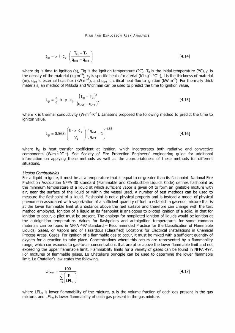
FF II RR EE AA NN DD EE XX PP LL OO SS II OO NN RR II SS KK AA NN AA LL YY SS II SS
critext
0igpig qq
TTclt [4.14]
where tig is time to ignition (s), Tig is the ignition temperature (ºC), T0 is the initial temperature (ºC), is the density of the material (kgm3), cp is specific heat of material (kJkg1ºC1), l is the thickness of material (m), qext is esternal heat flux (kWm2), and qcrit is critical heat flux to ignition (kWm2). For thermally thick materials, an method of Mikkola and Wichman can be used to predict the time to ignition value,
2critext
20ig
pigqq
TTck
4t
[4.15]
where k is thermal conductivity (Wm1K1). Janssens proposed the following method to predict the time to igniton value,
83.1
crit
ext2ig
pig 1
h
ck563.0t
[4.16]
where hig is heat transfer coefficient at ignition, which incorporates both radiative and convective components (Wm2ºC1). See Society of Fire Protection Engineers’ engineering guide for additional information on applying these methods as well as the appropriateness of these methods for different situations. Liquids Combustibles For a liquid to ignite, it must be at a temperature that is equal to or greater than its flashpoint. National Fire Protection Association NFPA 30 standard (Flammable and Combustible Liquids Code) defines flashpoint as the minimum temperature of a liquid at which sufficient vapor is given off to form an ignitable mixture with air, near the surface of the liquid or within the vessel used. A number of test methods can be used to measure the flashpoint of a liquid. Flashpoint is not a physical property and is instead a model of physical phenomena associated with vaporization of a sufficient quantity of fuel to establish a gaseous mixture that is at the lower flammable limit at a distance above the fuel surface and therefore can change with the test method employed. Ignition of a liquid at its flashpoint is analogous to piloted ignition of a solid, in that for ignition to occur, a pilot must be present. The analogy for nonpiloted ignition of liquids would be ignition at the autoignition temperature. Values for flashpoints and autoignition temperatures for some common materials can be found in NFPA 497 standard – Recommended Practice for the Classification of Flammable Liquids, Gases, or Vapors and of Hazardous (Classified) Locations for Electrical Installations in Chemical Process Areas. Gases. For ignition of a flammable gas to occur, it must be mixed with a sufficient quantity of oxygen for a reaction to take place. Concentrations where this occurs are represented by a flammability range, which corresponds to gas-to-air concentrations that are at or above the lower flammable limit and not exceeding the upper flammable limit. Flammability limits for a variety of gases can be found in NFPA 497. For mixtures of flammable gases, Le Chatelier’s principle can be used to determine the lower flammable limit. Le Chatelier’s law states the following,
n
1i i
im
LFLp
100LFL [4.17]
where LFLm is lower flammability of the mixture, pi is the volume fraction of each gas present in the gas mixture, and LFLm is lower flammability of each gas present in the gas mixture.

FF II RR EE AA NN DD EE XX PP LL OO SS II OO NN FF UU NN DD AA MM EE NN TT AA LL AA NN AA LL YY SS II SS
Fire Growth Following ignition, a fire might grow as it develops on the first item ignited or spreads to additional items. To determine whether spread would occur to adjacent items, the problem can be approached from the perspective of whether or not these items would ignite. For growth involving a single item, the fire could spread to unignited portions of the item. This could either lead to the entire item burning, or earlier ignited portions might burn out before the fire spreads to involve the entire item, such that the entire item is never fully involved. PP RR EE DD II CC TT II OO NN OO FF FF II RR EE EE FF FF EE CC TT SS The primary importance of the appropriate selection of the design fire’s growth is in obtaining a realistic prediction of detector and sprinkler activation, time to start of evacuation, and time to initial exposure of occupants. In 1972, Heskestad first proposed hat for the early fire growth period the assumption that fires grow according to a power law relation works well and is supported by experimental data. He suggested fire growth following the form,
nf tIQ [4.18]
where If is fire intensity coefficient (kWsn), t is time (s), and n is growth rate coefficient (n=1,2,3,...). Later, it was shown that for most flaming fires (except flammable liquids and some others) growth rate coefficient (n) is equal to 2, the so-called t-squared growth rate. A set of specific t-squared fires labeled slow, medium, and fast, with fire intensity coefficients such that the fires reached 1,000 Btus1 (1,055 kW) in 600, 300, and 150 seconds, respectively, were proposed for design of fire detection systems. Later, these specific growth curves and a fourth called “ultrafast”, which reaches 1,055 kW in 75 seconds, gained favor in general fire protection applications. The low growth (n 1) curves are appropriate for fires involving thick, solid objects (e.g., solid wood table, bedroom dresser, or cabinet). The medium growth curve (1 < n 2) is typical of solid fuels of lower density (e.g., upholstered furniture and mattresses). Fast fires are thin, combustible items (e.g., paper, cardboard boxes, draperies) and have high growth curves (n 2). Ultrafast fires are some flammable liquids, some older types of upholstered furniture and mattresses, or materials containing other highly volatile fuels. These t-squared curves represent fire growth starting with a reasonably large, flaming ignition source. With small sources, there is an incubation period before established flaming, which can influence the response of smoke detectors. During this incubation period, the fire may not significantly grow in size, although smoke would still be produced in quantities potentially sufficient to activate smoke detectors. This specific set of fire growth curves has been incorporated into several design methods, such as that for the design of fire detection systems in NFPA 72 (National Fire Alarm Code). They are also referenced as appropriate design fires in several international methods for performing alternative design analyses in Australia and Japan and in a product fire risk analysis method published in this country. Although in the Australian methodology the selection of growth curve is related to the fuel load (mass of combustible material per unit floor area), this is not justified, since the growth rate is related to the form, arrangement, and type of material and not simply its quantity. Steady Burning Where a fire scenario involves a fire in an enclosure, fire growth might continue until all the combustible items within the room are involved. Once this occurs, the rate of burning is influenced by one of two factors: (1) The available ventilation; (2) The available fuel. Calculation of fire temperatures within the room is easily accomplished by use of simple algebraic equations. Although computer models are frequently used in hazard analyses, they are generally no more accurate (and indeed may be less accurate) than simple hand calculations for prediction of temperature and burning rate during fully developed burning.10 For example, for postflashover fires, hand calculation methods are generally used to estimate compartment temperatures. SFPE’s engineering guide on fire exposures of structural elements provides calculation methods for predicting fire temperatures and burning rates in fully developed compartment fires. Some of these methods are based on an assumption of ventilation-limited burning, and others model fuel-controlled conditions. For most cases, the method developed by Law was

FF II RR EE AA NN DD EE XX PP LL OO SS II OO NN RR II SS KK AA NN AA LL YY SS II SS
found to provide bounding predictions when the factor was not used and the predicted burning duration was increased by a factor of 1.4. Law’s method is as follows,
05.0gm e1TT [4.19]
where Tgm is maximum compartment temperature (ºC), and factor is given by,
0s
f
AA
m
[4.20]
where mf is mass of fuel (kg), As is surface area of interior of enclosure (m2), Ao is area of ventilation opening (m2). The maximum compartment temperature (Tgm) is determined by the following expression,
00
s
00
s
gm
HA
A
HA
A1.0Exp1
6000T [4.21]
where H0 is height of ventilation opening (m). Law reports that the correlation for predicting burning rate is valid for condition,
60WD
HA
m 5.0
00
b
[4.22]
where mb is mass burning rate of fuel (kgs1), W is the width of wall containing ventilation opening (m), and D is depth of compartment (m). The mass burning rate of fuel (mb) is given by,
0H0AsA
036.0
00b e1DW
HA18.0m [4.23]
In some cases, it may only be desired to predict whether flashover is possible for a given fire scenario involving a fire in an enclosure. In such cases, the approach described in the section Prediction of Flashover can be used. Fire Decay All fires eventually decrease in size. A fire can decay for one of three reasons: consumption of available fuel, oxygen depletion, or suppression. Because the hazards posed during the decay phase are typically insignificant in comparison to the hazards posed during the fully developed phase, decay is typically omitted from analysis. An exception is in calculations involving structural fire resistance of concrete or insulated steel. Where test data are available, they might include decay. For fires with a predicted duration of less than 60 minutes, a decay rate of 10°C per minute can be used. In other case, a decay rate of 7°C per minute can be used. Decay could also occur in the event that a sprinkler system is present and activated. A simple assumption is that the fire immediately goes out, but this is not conservative. A National Institute of Standards and Technology (NIST) study documents a conservative exponential diminution in burning rate under the application of water from a sprinkler. Since the combustion efficiency is affected by the application of water, the use of values for soot and gas yields appropriate for post-flashover burning would represent the conservative approach in the absence of experimental data.

FF II RR EE AA NN DD EE XX PP LL OO SS II OO NN FF UU NN DD AA MM EE NN TT AA LL AA NN AA LL YY SS II SS
Prediction of Flashover Flashover occurs when a fire grows to such a size that it involves all combustible items within an enclosed room or space. Although occurrence of flashover is not a hazard in itself, flashover would affect the occurrence of other hazards. Several correlations are available to predict the minimum heat release rate necessary for flashover to occur in a room. The time at which flashover occurs can be estimated by determining when the fire is predicted to reach this minimum size. The following methods can be used to predict the minimum heat release rate necessary for flashover. The method of Babrauskas states that,
00min HA750Q [4.24]
where Qmin is minimum heat release rate required for flashover (kW). On other hand, the method of McCaffrey, Quintiere, and Harkleroad consider that the minimum heat release rate required for flashover (Qmin) is given by,
5.0
00Tmin HAAxk
610Q
[4.25]
where k is thermal conductivity of compartment surface (kWm1K1), x is the thickness of compartment surface (m), and AT is total area of compartment surfaces (m2). PP RR EE DD II CC TT II OO NN OO FF HH AA ZZ AA RR DD SS Fire is a dynamic process of interacting physics and chemistry, so predicting what is likely to happen under a given set of circumstances is daunting. The simplest predictive methods are algebraic equations. Computer models are used to automate fire hazard calculations and are particularly useful where many repeated calculations must be performed. Simple Fire Hazard Calculations Once the design fire curve has been developed, it is then possible to predict the hazards that would result. The types of hazards that might be of interest include the following: (1) Radiant heat flux, which affects the potential for ignition of materials or thermal injury to people. (2) Smoke production, which dictates the volume of smoke produced. (3) Fire plume and ceiling jet temperatures and velocities, which could cause weakening of exposed
structural elements (4) Species production, which affects the rate at which an untenable environment could be created. (5) Depth of upper layer, which can be used as a surrogate for an untenable environment. As was the case with the stages of design fire curves, it is not always necessary to quantify all of the hazards that result from a design fire scenario. The hazards that are quantified are a function of the goals of the analysis. For example, if the purpose of the analysis is to determine whether a thermally activated detection or suppression system activates, only the plume and ceiling jet temperatures and velocities might be determined. For analysis of a smoke control system, only the smoke production rate might be determined. A structural analysis might only require calculation of the heat transfer to the structure. An evacuation analysis might require quantification of all of the hazards listed. Radiant Heat Flux Radiant heat flux is a measure of the rate of radiative heat transfer per unit area. An example of radiant heat transfer is the heating that can be felt from exposure to the sun on a hot day (although the intensity of thermal radiation in sunlight is too small to be of concern from a fire standpoint). The radiant heat flux from a single burning item can be predicted as a function of the distance. For radiant heat fluxes resulting from fire gases, such as in a compartment fire, the radiant heat flux can be calculated if the gas temperature and the temperature of the target object are known by applying an equation similar to the Equation [1.139].

FF II RR EE AA NN DD EE XX PP LL OO SS II OO NN RR II SS KK AA NN AA LL YY SS II SS
41G
4GGef TTAq [1.139]
Smoke Production When calculating smoke production rates, smoke is usually defined as the products of combustion and the air entrained into the fire plume. Therefore, the amount of smoke produced is a function of the height above the fire. Fire Plumes and Ceiling Jet Temperatures and Velocities A fire will produce a plume of hot gas that will rise and contact the ceiling of a compartment, forming a ceiling jet. The temperature and velocity of a ceiling jet can be calculated in accordance with the following equations.
When 18.0Hx we have
35
32
H
Q9.16T
[4.26]
When 18.0Hx we have
HxQ
38.5T
32
[4.27]
When 15.0Hx we have
31
HQ
96.0U
[4.28]
When 15.0Hx we have
65
21
31
Hx
HQ195.0U
[4.29]
Where ΔT is temperature rise over ambient (°C), U is ceiling jet velocity (ms1), H is height above fire (m), x is horizontal distance from fire centerline (m), and Q is total heat release rate (kW). When using these equations, it must be cautioned that they are only valid for horizontal, unobstructed ceilings where there is no smoke layer present. In cases where a layer forms, higher temperature rises can be expected. Species Production Fires can create a number of products of combustion that can be toxic or corrosive, including carbon dioxide (CO2), water vapor (H2O), carbon monoxide (CO), and many others that vary with the fuel and burning conditions. Species production rates can be calculated from the following equation,
cjj H
QyG
[4.30]
where Gj is smoke production rate of species j (kg/sec), yj is yield fraction of species j, Q is heat release rate (kW), and Hc is heat of combustion of fuel (kJkg1). Yield fractions for several fuels are available in the Handbook of Fire Protection Engineering from Society Fire Protection Engineers (SFPE). Depth of Upper Layer As smoke is produced in a compartment, it forms a layer that descends as a function of time. This is analogous to filling a bowl of water. However, when applying this equation, it should be noted that the mass

FF II RR EE AA NN DD EE XX PP LL OO SS II OO NN FF UU NN DD AA MM EE NN TT AA LL AA NN AA LL YY SS II SS
production rate of smoke is not constant, since as the layer descends, the smoke production rate decreases due to the reduced vertical distance available to entrain air into the plume. Toxicity Toxic gases produced by a fire can incapacitate or kill people who are exposed to them. A commonly used approach to determine whether the fire-induced environment is potentially harmful to people exposed is the fractional effective dose (FED) model developed by Purser. This can be expressed as follows,
2O2COirrCNCOinc,g FfFFFF [4.31]
where Fg,inc is the fraction of an incapacitating dose of all asphyxiating gases, FCO is the fraction of an incapacitating dose of carbon mooxide (CO), FCN is the fraction of an incapacitating dose of HCN, Firr is the fraction of irritant dose, fCO2 is the multiplication factor for carbon dioxide (CO2) induced hyperventilation, and FO2 is the fraction of an incapacitating dose of low-oxygen hypoxia. The fraction of an incapacitating dose of all asphyxiating gases (Fg,inc) can be replaced by the fraction of an incapacitating dose of carbon dioxide (FCO2). Purser gives the following equations for calculation of the individual fractional effective doses,
30C102925.8
F036.1
CO4
CO
[4.32]
where CCO is the concentration of carbon monoxide (CO) expressed in parts per million,
43CNC
CN e2201
F [4.33]
where CCN is the concentration of HCN in parts per million added to the concentration of other nitriles minus the concentration of NO2. Firr is the fraction of the incapacitating dose from all incapacitating products (HCl, HBr, etc.),
52CO
2CO ef [4.34]
where CCO2 is the concentration of carbon dioxide in percent,
2OC9.2054.013.82O eF
[4.35]
where CO2 is the concentration of oxygen in percent,
2OC5189.01623.62CO eF
[4.36]
where CCO2 is the concentration of carbon dioxide (CO2) in percent. It should be noted that the above equations for fractional effective dose (FED) are based on a one minute exposure. For exposures to constant concentrations of fire products, the fractional effective dose can be determined by multiplying the value determined using the previous equations by the exposure time in minutes. For exposures where the concentrations vary with time, the total fractional effective dose can be calculated by discretizing the exposure (determining the average exposure at each one minute interval and summing the fractional effective dose determined for each one minute interval). It should be noted when applying the previous correlations that some populations are more susceptible than others to fire products (e.g. asthmatics, the old, and the young). Additionally, no single fractional effective dose (FED) value for design has been widely agreed on event for «average» populations. A report by the National Institute of Standards and Technology investigates this subject in detail.

FF II RR EE AA NN DD EE XX PP LL OO SS II OO NN RR II SS KK AA NN AA LL YY SS II SS
FF II RR EE CC OO MM PP UU TT EE RR MM OO DD EE LL SS A survey documented available models and calculation methods that could be applied to fire hazard analysis (FHA). The key to determining which are appropriate to a given situation and which are not is a thorough understanding of the assumptions and limitations of the individual model or calculation and how these relate to the situation being analyzed. Single-room models are appropriate where the conditions of interest are limited to a single, enclosed space. Where the area of interest involves more than one space, and especially where the area of interest extends beyond a single floor, multiple-compartment models should be used. This is because the interconnected spaces interact to influence fire development and flows. Many single-compartment models assume that the lower layer remains at ambient conditions (e.g. ASET). Since there is little mixing between layers in a closed space (unless there are mechanical systems), these models are appropriate. However, significant mixing can occur in doorways, so multiple-compartment models should allow the lower layer to be contaminated by energy and mass. The model should include the limitation of burning by available oxygen. This is straightforward to implement (based on the oxygen consumption principle) and is crucial to obtaining an accurate prediction for ventilation-controlled burning. For multiple-compartment models, it is equally important for the model to track unburned fuel and allow it to burn when it encounters sufficient oxygen and temperature. Without these features, the model concentrates the combustion in the room of origin, overpredicting conditions there and underpredicting conditions in other spaces. Heat transfer calculations take up a lot of computer time, so many models take a shortcut. The most common is the use of a constant «heat loss fraction», which is user-selectable (e.g. ASET or CCFM). The problem is that heat loss can vary during the course of the fire. Another problem can occur in tall spaces, for example, atria. The major source of gas expansion and energy and mass dilution is entrainment of ambient air into the fire plume (see Figure 1.12). It can be argued that in a very tall plume, this entrainment is constrained. However, most models do not include this constraint, which can lead to an underestimate of the temperature and smoke density and an overestimate of the layer volume and filling rate, the combination of which may give predictions of available safe egress times that are either greater or less than the correct value. In the model CFAST, this constraint is implemented by stopping entrainment when the plume temperature drops to within 1°C of the temperature just outside the plume, where buoyancy ceases. Only models that are rigorously documented should be allowed in any application involving public health, safety, or welfare, such as in code enforcement or litigation. This means that the model should be supplied with a technical reference guide that includes a detailed description of the included physics and chemistry, with proper literature references; a listing of all assumptions and limitations of the model; and estimates of the accuracy of the resulting predictions, based on comparisons to experimental data. Public exposure and review of the exact basis for a model’s calculations, internal constants, and assumptions are necessary for it to have credibility in a regulatory application. Even if the model is correct, the results can be seriously in error if the data that are input to the model do not represent the condition being analyzed. The fire hazard analysis (FHA) should include a listing of all data values used, their source (i.e. what apparatus or test method was employed and what organization ran the test and published the data), and some discussion of the uncertainty of the data and its result on the conclusions. The National Institute of Standards and Technology’s (NIST) website contains a section of well-documented data for use in calculations, called called FASTDATA, is available from National Institute of Standards and Technology on a CD-ROM (see the URL above for information). Egress Models The prediction of the time needed by the facility occupants to evacuate to a safe area can be performed and compared to the predicted available safe egress time. Whether the evacuation calculation is done by model or hand calculation, it must account for several crucial factors. First, unless the occupants see the actual fire, time is required for detection and notification before the evacuation process can begin. Next, unless the information is compelling (such as seeing the actual fire), it takes time for people to decide to take action. The action they choose may or may not be evacuation. Finally, the movement begins. All of these factors require time, and that is the critical factor. No matter how the calculation is done, all of the factors must be included in the analysis to obtain a complete picture.The process of emergency evacuation of people follows the general concepts of traffic flow. A number of models perform such calculations and may be appropriate for use in certain occupancies. Most of these models do not account for behavior and the interaction of people (providing assistance) during the event. The literature reports incidents of providing assistance to

FF II RR EE AA NN DD EE XX PP LL OO SS II OO NN FF UU NN DD AA MM EE NN TT AA LL AA NN AA LL YY SS II SS
disabled persons, again especially in office settings. If such behavior is expected, it should be included, as it can result in significant delays in evacuating a building. Crowded conditions, as well as smoke density, can result in reduced walking speeds. A person’s walking speed decreases in dense smoke until he or she moves as if blindfolded. Care should be exercised in using models relative to how they select the path (usually the shortest path) that the person travels. Some models are optimization calculations that give the best possible performance. Analyzing the Impact of Exposure In most cases, the exposure will be to people, and the methods used to assess the impacts of exposure of people to heat and combustion gases involve the application of combustion toxicology models. The HAZARD I software package contains the only toxicological computer model, called TENAB, that is based on research at National Institute of Standards and Technology on lethality to rats and on incapacitation of monkeys. TENAB accounts for the variation in exposure to combustion products as people move through a facility or closed space, by reading the concentrations from the fire model in the occupied space during the time the person is in that space. If the person moves into a space with a lower concentration of carbon monoxide, the accumulated dose can decrease. Details such as these ensure that the results are reasonable. Assessing the impact of exposure to sensitive equipment is more difficult, since little data exist in the literature on the effects of smoke exposure on such equipment. Of particular importance here is the existence of acid gases in smoke, which are corrosive and especially harmful to electronics. Fuels containing chlorine (e.g. polyvinyl chlorides) have been studied. However, unless the equipment is close to the fire, acid gases, especially hydrochloric acid (HCl), deposit on the walls and lower the concentration to which the equipment may be exposed. CFAST in the HAZARD I package contains a routine that models this process and the associated diminution of hydrochloric acid concentration. Accounting for Uncertainty Uncertainty analysis refers to dealing with the unknowns and variation inherent in any prediction. In the calculations, this uncertainty is derived from assumptions in the models and from the representativeness of the input data. In evacuation calculations, there is the added variability of any population of real people. In facility (or building) designs and codes, the classic method of treating uncertainty is with safety factors. A sufficient safety factor is applied such that, if all of the uncertainty resulted in error in the same direction, the result would still provide an acceptable solution. In the prediction of fire development or filling time, the intent is to select design fires that provide a worst likely scenario. Thus a safety factor is not needed here, unless assumptions or data are used to which the predicted result is very sensitive. The fire hazard analysis (FHA) report should include a discussion of uncertainty. This discussion should address the representativeness of the data used and the sensitivity of the results to data and assumptions made. If the sensitivity is not readily apparent, a sensitivity analysis (i.e. varying the data to the limits and seeing whether the conclusions change) should be performed. This is also a good time to justify the appropriateness of the model or calculation method. Final Review If a model or calculation produces a result that seems counter-intuitive, there is probably something wrong. Cases have been seen in which the model clearly produced a wrong answer (e.g. the temperature predicted approached the surface temperature of the sun), and there have been others in which it initially looked wrong but was not (e.g. a dropping temperature in a space adjacent to a room with a growing fire was caused by cold air from outdoors being drawn in an open door). Conversely, if the result is consistent with logic, sense, and experience, it is probably correct. This is also a good time to consider whether the analysis addressed all of the important scenarios and likely events. Were all the assumptions justified and were uncertainties addressed sufficiently to provide a comfort level similar to that obtained when the plan review shows that all code requirements have been met?
BB II BB LL II OO GG RR AA PP HH YY Bukowski, R. W., A review of international fire risk prediction methods, Interflam ‘93, Interscience Communications, Ltd., London, UK, 1993.

FF II RR EE AA NN DD EE XX PP LL OO SS II OO NN RR II SS KK AA NN AA LL YY SS II SS
D. C. Hamilton and W. R. Morgan. Radiant interchange configuration factors. NACA Technical Note 2836, National Advisory Committee for Aeronautics, Washington, D.C., 1952. Department of Housing and Urban Development. Safety considerations in siting housing projects, 1975. HUD Report 0050137. Department of Housing and Urban Development. Urban development siting with respect to hazardous commercial and industrial facilities, April 1982. HUD Report HUD-777-CPD. Drysdale, D., An introduction to fire dynamics, 2nd ed., Wiley, Chichester, UK, 1998. Fire protection handbook. National Fire Protection Association, Quincy, Massachusetts, 18th edition, 1997. H. Koseki and T. Yumoto. Air entrainment and thermal radiation from heptane pool fires. Fire Technology, 24, February 1988. J. C. Yang, A. Hamins, and T. Kashiwagi. Estimate of the effect of scale on radiative heat loss fraction and combustion efficiency. Combustion Science and Technology, 96:183–188, 1994. K. S. Mudan and P. A. Croce. SFPE Handbook, Chapter: Fire hazard calculations for large open hydrocarbon fires. National Fire Protection Association, Quincy, Massachusetts, 2nd edition, 1995. N. Takahashi, H. Koseki, and T. Hirano. Temporal and spatial characteristics of radiation from large pool V. Babrauskas. SFPE Handbook, Chapter: Burning rates. National Fire Protection Association, Quincy, Massachusetts, 2nd edition, 1995. Purser, D., Toxicity assessment of combustion products, SFPE Handbook of Fire Protection Engineering, 3rd ed., P. J. DiNenno et al. (Eds.), National Fire Protection Association Quincy, MA, 2002. Schifiliti, R. P., Meacham, B. J., and Custer, R. L. P., Design of detection systems, SFPE Handbook of Fire Protection Engineering, National Fire Protection Association, Quincy, MA, 2002. Society of Fire Professional Engineers (SFPE), Engineering guide to performance-based fire protection, National Fire Protection Association, Quincy, MA, 2006. Society of Fire Protection Engineers, Bethesda, Maryland. Engineering guide for assessing flame radiation to external targets from pool fires, June 1999. Tewarson, A., Generation of heat and chemical compounds in fires, SFPE Handbook of Fire Protection Engineering, 3rd ed., P. J. DiNenno et al. (Eds.), National Fire Protection Association, Quincy, MA, 2002. W. D. Walton. In-situ burning of oil spills: Meso-scale experiments and analysis. In Proceedings of the 16th Arctic and Marine Oil Spill Program (AMOP) Technical Seminar, pages 679–734. Environment Canada, Emergencies Science Division, Ottawa, Ontario, Canada, June 1993.

FF II RR EE AA NN DD EE XX PP LL OO SS II OO NN FF UU NN DD AA MM EE NN TT AA LL AA NN AA LL YY SS II SS
SS ee cc tt ii oo nn 55
FF IIRREE HHAAZZAARRDDSS CCLLAASSSS II FF IICCAATT IIOONN
CC LL AA SS SS II FF II CC AA TT II OO NN OO FF OO CC CC UU PP AA NN CC II EE SS The principal occupancy classifications are light hazard, ordinary hazard, and extra hazard. Listed below are the classifications with examples of common occupancies listed under each. The basic hazard classification of an occupancy does not define the fire hazard present in all areas of that occupancy. If more hazardous processes or areas exist within a given occupancy, protect these areas in accordance with the fire protection requirements pertaining to the hazard classification of that area. Determine the classification for unlisted occupancies from the definitions or by comparison with one of the listed occupancies. LL II GG HH TT HH AA ZZ AA RR DD OO CC CC UU PP AA NN CC II EE SS Occupancies or portions of occupancies where the quantity and combustibility of the contents are low and fires with relatively low rates of heat release are expected. Small, scattered amounts of flammable liquids in closed containers are allowable in quantities not exceeding 20 L (5 gal) per fire area. This classification includes but is not limited to the following occupancies: (1) Churches and chapels; (2) Gymnasiums; (3) Clinics (dental, outpatient, patient areas only); (4) Hospitals; (5) Data processing areas; (6) Mess areas; (7) Dispensaries (patient areas only); (8) Drill halls (not used for storage or exhibition); (9) Disciplinary barracks; (10) Offices; (11) Child development centers. OO RR DD II NN AA RR YY HH AA ZZ AA RR DD –– GG RR OO UU PP 11 OO CC CC UU PP AA NN CC II EE SS Occupancies or portions of occupancies where combustibility is low, quantity of combustibles is moderate, stockpiles of combustibles do not exceed 2.5 m (8 ft), and fires with moderate rates of heat release are expected. Modest, scattered amounts of flammable liquid, in closed containers are allowable in quantities not to exceed 75 L (20 gal) per fire area. This classification includes but is not limited to the following occupancies: (1) Armories; (2) Sheet metal shops; (3) Bowling alleys; (4) Ship fitting shops; (5) Clubs (officer, enlisted personnel, etc.); (6) Kitchens and bakery; (7) Small stores; (8) Theaters and auditoriums; (9) Welding shops; (10) Forge shops; (11) Laundries; (12) Automobile parking garage; (13) Electronics assembly and repair. OO RR DD II NN AA RR YY HH AA ZZ AA RR DD –– GG RR OO UU PP 22 OO CC CC UU PP AA NN CC II EE SS Occupancies or portion of occupancies where quantity and combustibility of contents is moderate, stockpiles do not exceed 3.7 m (12 ft), and fires with moderate rate of heat release are expected. Moderate, scattered amounts of flammable liquids in closed containers are allowable in quantities not to exceed 200 L (50 gal)

FF II RR EE AA NN DD EE XX PP LL OO SS II OO NN RR II SS KK AA NN AA LL YY SS II SS
per fire area. Small amounts of flammable liquids may be exposed as required by normal operations. This classification includes but is not limited to the following occupancies: (1) Commissaries; (2) Exchanges; (3) Aviation Depots; (4) Boiler rooms; (5) Electrical maintenance shops; (6) Engine and generator rooms; (7) Laboratories; (8) Refrigeration and air compressor rooms; (9) Switchgear rooms; (10) Machine rooms; (11) Printing shops (using inks having flash points above 44ºC (110ºF); (12) Libraries; (13) Piers and wharves; (14) Vehicle repair garages; (15) Woodworking shops. SS PP EE CC II AA LL OO CC CC UU PP AA NN CC II EE SS Special occupancies are facilities or areas that cannot be assigned a specific classification because of special protection requirements. This classification includes but is not limited to the following occupancies: (1) Flammable and combustible liquids; (2) Aircraft hangars; (3) Engine test cells; (4) Missile assembly; (5) Ordnance plants; (6) Rubber tire storage; (7) Warehouses (piled or rack storage); (8) Foam rubber or plastic storage.
HH AA ZZ AA RR DD OO UU SS AA RR EE AA CC LL AA SS SS II FF II CC AA TT II OO NN The concept of assessing and limiting the risk associated with areas where potentially explosive atmospheres may be present is referred to as area classification. Hazardous area classification (HAC) assessment is a probability (likelihood) analysis and risk assessment evaluation of a manufacturing or process area processing a potentially flammable atmosphere that focuses exclusively on minimizing or eliminating energy as a potential ignition source. Hazardous area classification is not intended to be a secondary line of defense against poor process design, poor facility and euipment maintenance, faulty equipment operation, or catastrophic vapor releases. Hazardous areas are divided into threee distinct classes that totally depend on the material type that is encountered in the process. CC LL AA SS SS II AA RR EE AA SS These are locations where flammable gases or vapors are or may be present in the air in quantities sufficient to produce an explosive or ignitable mixture. In Class I areas that utilize the division concept methodology, two distinct divisions are predicted on the operational interpretation of normal versus abnormal and frequent versu infrequent. Division I locations where ignitable concentrations of flammable gases r vapors can exist sre due to: (1) Under normal operating conditions. (2) Frequently because of maintenance or repair. (3) Frequent leakage. (4) Below grade where adequate ventilation does not exist. (5) When releases from faulty process equipment operations result in the simiultaneous failure of equipment
and machinery.

FF II RR EE AA NN DD EE XX PP LL OO SS II OO NN FF UU NN DD AA MM EE NN TT AA LL AA NN AA LL YY SS II SS
Division II locations here ignitable concentrations of flammable gases or vapors can exist are: Failure of closed containment systems. Abnormal operation or failure of processing and ventilation equipment. Area is adjacent to a Division I location. In Class I areas that utilize the division concept methodolog, four distinct groups are based solely on the liquid or gas ease of ignitability and its corresponding range of flammability or explosivity (ER, range of explosivity in volume percent): (1) Group A – Atmospheres that contain acetylene (2.5% UER 100%). (2) Group B – Fammable gas (eg. hydrogen) or vapor atmospheres having either a maximum experimental
safe gap (MESG) less than orequal to 0.4 mm or a minimum ignition current (MIC) ratio less than or equal to 0.40 mm (4.0% ER 75.0%).
(3) Group C – Fammable gas (eg. ethylene) or vapor atmospheres having either a maximum experimental safe gap (MESG) greater than 0.45 mmm and less than orequal to 0.75 mm or a minimum ignition current (MIC) ratio greater than 0.40 mm and less than or equal to 0.80 mm (2.7% ER 36.0%).
(4) Group D – Fammable gas (eg. propane) or vapor atmospheres having either a maximum experimental safe gap (MESG) greater than 0.75 mmm or an minimum ignition current (MIC) ratio greater than 0.80 mm (2.1% ER 9.5%).
The explosive ranges are base on normal atmospheric pressure and temperature. As the mixture temperature increases, the flammable range shifts downward. As the mixture temperature decreases, the flammable range shifts upward. It can be easily determined from examining the above statements that the mixture volatility is much greater for Group A mixtures compared to Group D. Classes of combustible liquids include Class II which is any liquid with a flash point greater than 100ºF (37.8ºC) and less than 140ºF (60ºC). Class III liquids are liquids with a flash point greater than 140ºF (60ºC). Class III liquids are further divided as either Class III-A liquids or Class III-B liquids. Class III-A liquids have flash point greater than 140ºF ()60ºC and less than 200ºF (93.3ºC). Class III-B liquids have a flash point greater than 200ºF (93.3ºC). CC LL AA SS SS II II AA RR EE AA SS These are hazardous locations because combustibledust is present. Combustible dust is defined as any solid material 420 microns or less in diameter that present a fie or an explosion hazard when dispersed in air. Like Class I areas, Class II areas are also divided into two distinct divisions that again depend on operational interpretation of normal versus abnormal conditions. Division I is a location where combustible dust is present in the air: (1) Under normal operating conditions, in quantities sufficient to produce an explosive or ignitable mixture. (2) The dust is electrically conductive. Dusts are considered to be electrically conductive if the electrical
resistivity of the solid material from which the dust is formed has a value of less than 105 cm. (3) Releases from faulty operation of process equipment result in the simultaneous failure of the electrical
equipment, causing the electrical equipment to become a source of ignition. Division II is a location where combustible dust is: (1) Present in the air only under abnormal operating conditions in quantities sufficient to produce an
explosive or ignitable mixture. (2) Accumulations are normally insufficient to interfere with the normal operation of the electrical equipment
or other apparatus, but combustible dust could be in suspensions in the air due to infrequent process equipment malfunctions.
(3) Accumulations on, in, or in the vicinity of the electrical equipment could be sufficient to interfere with the safe dissipation of heat from electrical equipment, or could be ignitable by abnormal operation or electrical equipment failure.
In Class II areas three distinct goups are based primarily on the physical characteristics of the dust: (1) Group E – Atmospheres that contain combustible metal dusts, including aluminium, magnesium, and
their commercial alloys, or other combusible dusts whose particle size, abrasiveness and conductivity present similar hazards in the use of electrical equipment.

FF II RR EE AA NN DD EE XX PP LL OO SS II OO NN RR II SS KK AA NN AA LL YY SS II SS
(2) Group F – Atmospheres that contain combustible carbonaceous dusts that have more than 8% total entrapped volatiles or that have been sensitized by other materials so that they present an explosion hazard. Representative combustible dusts that fall into this grouping are coal, carbon black, charcoal and coke.
(3) Group G – Atmospheres containing other combustible dusts, including flour, grain, wood flur, plastic and chemicals.
Explosion severity is a measure of the damage potential of the energy release by a dust explosion. The United States Bureau of Mines (USBM) has defined the equation for calculating explosion severity (Sexp) as,
IPmax
IIPmaxexp P
PS
[5.1]
where Pmax is the maximum explosion pressure (bar), and P is the maximum rate od pressure rise (bars-1); subscript I refers to the values used for Pittsburgh seam coal (Pmax is 8.1 bar, P is 214 bars-1), and subscript II refers to the values for the specific dust in question. Ignition sensitivity is a measure of the ease by which a cloud of combustible dust can be ignited. The United States Bureau of Mines has defined the equation for calculating ignition sensitivity (Isen) as,
IIminexp,min,igmin,ig
Iminexp,min,igmin,igsen MET
METI
[5.2]
where Tig,min is the minimum gnition temperature (ºC), Eig,min is the minimum ignition energy (mJ, milijoule), and Mexp,min is the minimum explosion concentration (gm-3 or gpcm); subscript I refers to the values used for Pittsburgh seam coal (Tig,min is 591ºC, Eig,min is 160 mJ, Mexp,min is 70 gm-3), and subscript II refers to the values for the specific dust in question. Dusts that have ignition sensitivities equal to or greater than o.2 or explosion severities equal to or graeter than 0.5 are considered to have enough volatility to warrant locations processing these dusts to be classified. The material published by United States Bureau of Mines (USBM) is no longer in print and copies are hard to find. CC LL AA SS SS II II II AA RR EE AA SS These are hazardous locations because easily ignitable fibers and flyings are present. In Class III areas, there are no goupings as in Class I and Class II areas. There are, however, divisions that are based on how the material is processed. Division I is a location where easily ignitable fibers producing combustible flyings are handled, manufactured or used. Division II is a location where easily ignitable fibers are stored or handled other than in the manufacturing process. AA RR EE AA CC LL AA SS SS II FF II CC AA TT II OO NN AA SS SS EE SS SS MM EE NN TT Once the risk assessment methodology is developed, then the actual process of classifying the area is ready to begin. A typical assssment study will include seven basic steps: (1) Step I – Obtain the required documentation that was determined from the assessment methodology.
Provide a lower level view of the process for equipment identification and process arrangements. (2) Step II – Field-survey the area in question to determine if the plot plans are accurate and verify location
of all point sourcesof emissions. (3) Step III – Determine the classified area extent that surrounds each point source will play in the overall
composite area classification diagram. The extent of classification diagrams should come from NFPA 497 (National Fire Protection Association) for petrochemical applications, API RP500 (American Petroleum Institute) for petroleum refinery applications or gas dispersion modelling software tools. Gas and vapor dispersion modeling software should be utilized when one out of these three scenarios exists: Extreme process conditions are encountered such as large flowrates (> 250 gpm), pressures (> 275 psig), and liquids with a vapor pressure above 70 psia at operating temperature. Combustibe liquids are heated to temperatures above 100ºF (37.8ºC) of their respective flash points. The stream composition is a complex mixture of hydrocarbons.

FF II RR EE AA NN DD EE XX PP LL OO SS II OO NN FF UU NN DD AA MM EE NN TT AA LL AA NN AA LL YY SS II SS
(4) Step IV – Develop the composite area classification plan drawing that embellishes the contribution of all
point sources. (5) Step V – Develop elevation drawingsto provide clarity where here are emission sources located in
multilevel process structures. A lan view will be required for each level in the process structre. (6) Step VI – Conduct the compliance audit. (7) Step VII – Create a detailed assessment report that documents the following informaton: the rationale
used to classify the areas; the critical process material information usuall obtained from the material safety data sheets (MSDS); a detailed listing of all point sources of emissions that appear on the drawings; special out-of-the-ordinary exceptions that were taken when classifying a particular location; the results or findings obtained from the compliance audit; a vapor dispersion modeling graph.
All area classification documentation should be placed under the protection of the facilities management of change process control. As modifications are made to the facility, these documents should be reviewed to verify the impact of these modifications. PP RR OO TT EE CC TT II OO NN MM EE TT HH OO DD SS AA NN DD HH AA ZZ AA RR DD RR EE DD UU CC TT II OO NN Hazard reduction is where a facility reduces the probability or risk of significant property damage and loss of life as the result of an explosion or a fire. It helps ensure that installing equipment or machinery in a hazardous location does not significantly raise the risk or probability of an explosion or fire. This is the point where steps are taken to provide compliance with the area classification assessment. Mitigation options are discussed and corresponding action items are carried out. In Class I areas it is important to follow the key protection methods: (1) Physically isolate the hazard by placing or relocating the arc-producing electrical devices to a
nonhazardous area; this is an attractive option when approved equipment for the classified area is not readily or commercially available.
(2) Confining explosion is the most common and widely accepted protection method. It deploys the use of devices that are vendor-certified, through listing or labeling, as explosion-proof. Explosion-proof means that the device enclosure is designed and tested in a manner that guarantees if a flammable vapor enters the enclosure and is ignited by an electrical arc or a hot surface within the enclosure, the resulting explosion is contained within the enclosure. The electrical apparatus contained within the enclosure should still be operational.
(3) Energy limiting is known as an intrinsic safety measure, that prevents ignition by limiting the released energy resulting from wiring and component failures or faults. Underwriters Laboratory (UL) listed intrinsically safe electrical devices are incapapble of releasing enough energy under normal or abnormal conditions to cause ignition of a specific hazardous atmosphere in its most easily ignitable concentrations.
(4) Hermetically sealed types of protection ensure that arc or heat-producing devices are sealed against the intrusion of the hazardous vapor.
(5) Pressurization is the process of supplying an enclosure with a protective gas with or without continuous flow to prevent the entrance of a flammable vapor, combustible dust or ignitable fiber.
(6) Purging is the process of supplying an enclosure with a protective gas at a sufficient flow and positive pressure to reduce the concentration of any flammable vapor initially present to a safe level.
In Class II areas it is important to follow the key protection methods: (1) Physically isolate the hazard in the same manner as for Class I areas. (2) Utilization of dust ignition-proof equipment requires that the enclosure is dust-tight, and the enclosure is
constructed so that heat generated inside will not ignite a dust layer on or a combustible cloud surrounding the enclosure.
(3) Purging may be used as long as the NFPA 496 requirements are followed. (4) Energy limiting is at the same level of protection as in Class I areas. In Class III areas are employed the same methods that were utilized for Class II areas. The basic requirement is to make use of dust-tight enclosures for all normal arc-producing electrical devices and electrostatic producing devices.
FF II RR EE AA NN DD EE XX PP LL OO SS II OO NN RR II SS KK AA NN AA LL YY SS II SS
BB II BB LL II OO GG RR AA PP HH YY NFPA 30, Flammable and combustible liquids code, 2000 Ed., NFPA, Quincy, Massachusetts, 2000. NFPA 496, Standard for purged and pressurized enclosures for electrical equipment, 1998 Ed., NFPA, Quincy, Massachusetts, 1998. NFPA 497, Recommended practice for the classification of flammable liquids, gases or vapors and of hazardous (classified) locations for electrical installations in chemical process areas, 1997 Ed., NFPA, Quincy, Massachusetts, 1997. NFPA 499, Recommended practice for the classification of combustible dusts and of hazardous (classified) locations for electrical installations in chemical process areas, 19997 Ed., NFPA, Quincy, Massachusetts, 1997. ANSI / API PR5000, Recommended practice for classification of locations for electrical installations at petroleum facilities classified as Class I, Division I and Division II, 2nd Ed., API Publishing Services, Washington, DC, 1997. ISA-12.10, Area classification in hazardous (classified) dust locations, ISA, Research Triangle Park, North Carolina, 1988. Cashdollar, K. M. Hertzberg and R. Conti, RI-8988 Bureau of Mine Report of Investigations – 1985, Electrical ignition energies and thermal autoignition temperatures of evaluating explosion hazards of dusts, United States Department of the Interior, 1985.
FF II RR EE AA NN DD EE XX PP LL OO SS II OO NN FF UU NN DD AA MM EE NN TT AA LL AA NN AA LL YY SS II SS
SS ee cc tt ii oo nn 66
EENNGGIINNEEEERR IINNGG EECCOONNOOMMIICCSS
II NN TT RR OO DD UU CC TT II OO NN Engineering economics is the application of economic techniques to the evaluation of design and engineering alternatives. The role of engineering economics is to assess the appropriateness of a given project, estimate its value, and justify it from an engineering standpoint. This section discusses the time value of money and other cash-flow concepts, such as compound and continuous interest. It continues with economic practices and techniques used to evaluate and optimize decisions on selection of fire safety strategies. The final section expands on the principles of benefit-cost analysis. An in-depth treatment of the practices and techniques covered in this compilation is available in the ASTM compilation of standards on facility economics. The ASTM compilation also includes case illustrations showing how to apply the practices and techniques to investment decisions. A broader perspective on the application of engineering economics to fire protection engineering can be found in The Economics of Fire Protection by Ramachandran. This work is intended as being part of this textbook for fire protection engineers. CC AA SS HH -- FF LL OO WW CC OO NN CC EE PP TT SS Cash flow is the stream of monetary values – costs (inputs) and benefits (outputs) – resulting from a project investment. Time Value of Money The following are reasons why 1,000 monetary value today is worth more than 1,000 one year from today: (1) Inflation; (2) Risk; (3) Cost of money. Of these, the cost of money is the most predictable, and, hence, it is the essential component of economic analysis. Cost of money is represented by (1) money paid for the use of borrowed money, or (2) return on investment. Cost of money is determined by an interest rate. Time value of money is defined as the time-dependent value of money stemming both from changes in the purchasing power of money (inflation or deflation) and from the real earning potential of alternative investments over time. Cash-Flow Diagrams It is difficult to solve a problem if you cannot see it. The easiest way to approach problems in economic analysis is to draw a picture. The picture should show three things: (1) A time interval divided into an appropriate number of equal periods; (2) All cash outflows (deposits, expenditures, etc.) in each period; (3) All cash inflows (withdrawals, income, etc.) for each period. Unless otherwise indicated, all such cash flows are considered to occur at the end of their respective periods. Notation To simplify the subject of economic analysis, symbols are introduced to represent types of cash flows and interest factors. The symbols used in this chapter conform to ANSI Z94; however, not all practitioners follow this standard convention, and care must be taken to avoid confusion when reading the literature. The following symbols will be used here: (1) P is present sum of money; (2) F is future sum of money; (3) N is number of interest periods; (4) i is interest rate per period (%).

FF II RR EE AA NN DD EE XX PP LL OO SS II OO NN RR II SS KK AA NN AA LL YY SS II SS
II NN TT EE RR EE SS TT FF AA CC TT OO RR SS Interest factors are multiplicative numbers calculated from interest formulas for given interest rates and periods. They are used to convert cash flows occurring at different times to a common time. The functional formats used to represent these factors are taken from ANSI Z94. Interest Calculations Interest is the money paid for the use of borrowed money or the return on invested capital. The economic cost of construction, installation, ownership, or operation can be estimated correctly only by including a factor for the economic cost of money. Compound Amount Factor In the formula for finding the future value (F) of a sum of money with compound interest, the mathematical expression,
ni1 [6.1]
is referred to as the compound amount factor, represented by the functional format
n,i,PF
. Thus,
n,i,
PF
PF [6.2]
Present Worth Present worth (P) is the value found by discounting future cash flows to the present or base time. Discounting is the inverse of compounding is determining a present amount which will yield a specified future sum. This process is referred to as discounting. The equation for discounting is found readily by using the compounding equation to solve for present worth in terms of future value,
ni1FP [6.3] Interest Periods Normally, but not always, the interest period is taken as 1 year. There may be subperiods of quarters, months, weeks, and so forth. It is generally assumed that interest is compounded annually. However, interest may be compounded more frequently. When this occurs, there is a nominal interest (in) or annual percentage rate and an effective interest (ie), which is the figure used in calculations. For example, a savings bank may offer 5 percent interest compounded quarterly, which is not the same as 5 percent per year. A nominal rate of 5 percent compounded quarterly is the same as 1.25 percent every three months or an effective rate of 5.1 percent per year. If in is the nominal interest rate and m is number of periods per year, then the effective interest rate (ie) is given by,
1mi
1im
ne
[6.4]
Series Payments Life would be simpler if all financial transactions were in single lump-sum payments, now or at some time in the future. However, most situations involve a series of regular payments, for example, car loans and mortgages. Given a series of regular payments, what will they be worth at some future time? Let A being the amount of a regular end-of-period payment. Then, note that each payment (A) is compounded for a different period of time. The first payment will be compounded for a number of periods greater than periods of one year,
1nei1AF [6.5]

FF II RR EE AA NN DD EE XX PP LL OO SS II OO NN FF UU NN DD AA MM EE NN TT AA LL AA NN AA LL YY SS II SS
and the second payment for (n2) periods,
2nei1AF [6.6]
and so forth. Thus the total future value is given by,
e
n
i1i1
AF
[6.7]
The interest expression in this equation is known as the series compound amount factor. Sinking Fund Factor The process corresponding to the inverse of series compounding is referred to as a sinking fund; that is, what size regular series payments are necessary to acquire a given future amount? Solving the series compound amount equation for each payment (A),
1i1
iFA
ne
[6.8]
Capital Recovery Factor It is also important to be able to relate regular periodic payments to their present worth; the interest expression is known as the capital recovery factor, since the equation defines a regular income necessary to recover a capital investment. The symbolic equation becomes,
1i1
i1iPA
n
ne [6.9]
Series Present Worth Factor As with the other factors, there is a corresponding inverse to the capital recovery factor. The series present worth factor is found by solving the capital recovery equation for pesent worth value (P).
ne
n
i1i
1i1AP [6.10]
OO TT HH EE RR II NN TT EE RR EE SS TT CC AA LL CC UU LL AA TT II OO NN CC OO NN CC EE PP TT SS Additional concepts involved in interest calculations include continuous cash flow, capitalized costs, beginning of period payments, and gradients. Perhaps the most useful function of continuous interest is its application to situations where the flow of money is of a continuous nature. Continuous cash flow is representative for: (1) A series of regular payments for which the interval between payments is very short. (2) A disbursement at some unknown time (which is then considered to be spread out over the economic
period). Factors for calculating present or future worth of a series of annual amounts, representing the total of a continuous cash flow throughout the year, may be derived by integrating corresponding continuous interest factors over the number of years the flow is maintained. Continuous cash flow is an appropriate way to handle economic evaluations of risk, for example, the present value of an annual expected loss. Capitalized Costs Sometimes there are considerations, such as some public works projects, which are considered to last indefinitely and thereby provide perpetual service. For example, how much should a community be willing to
FF II RR EE AA NN DD EE XX PP LL OO SS II OO NN RR II SS KK AA NN AA LL YY SS II SS
invest in a reservoir which will reduce fire insurance costs by some annual amount? Taking the limit of the series present worth factor as the number of periods goes to infinity gives the reciprocal of the interest rate. Thus, capitalized costs are just the annual amount divided by the interest rate. When expressed as an amount required to produce a fixed yield in perpetuity, it is sometimes referred to as an annuity. Beginning-of-Period Payments Most returns on investment (cash inflows) occur at the end of the period during which they accrued. For example, a bank computes and pays interest at the end of the interest period. On the other hand, most disbursements (cash outflows) occur at the beginning of the period (e.g. insurance premiums). When dealing with beginning-of-period payments, it is necessary to make adjustments. One method of adjustment for beginning-of-period payments is to calculate a separate set of factors. Another way is to logically interpret the effect of beginning-of-period payments for a particular problem, for example, treating the first payment as a present value. The important thing is to recognize that such variations can affect economic analysis. Gradients It occasionally becomes necessary to treat the case of a cash flow which regularly increases or decreases at each period. Such patterned changes in cash flow are called gradients. They may be a constant amount (linear or arithmetic progression), or they may be a constant percentage (exponential or geometric progression). CC OO MM PP AA RR II SS OO NN OO FF AA LL TT EE RR NN AA TT II VV EE SS Most decisions are based on economic criteria. Investments are unattractive, unless it seems likely they will be recovered with interest. Economic decisions can be divided into two classes: (1) Income-expansion, that is, the objective of capitalism. (2) Cost-reduction, the basis of profitability. Fire protection engineering economic analysis is primarily concerned with cost-reduction decisions, finding the least expensive way to fulfill certain requirements, or minimizing the sum of expected fire losses plus investment in fire protection. There are four common methods of comparing alternative investments: (1) present worth, (2) annual cost, (3) rate of return, and (4) benefit-cost analysis. Each of these is dependent on a selected interest rate or discount rate to adjust cash flows at different points in time. Discount Rate The term discount rate is often used for the interest rate when comparing alternative projects or strategies. During the selection of discount rate, if costs and benefits accrue equally over the life of a project or strategy, the selection of discount rate will have little impact on the estimated benefit-cost ratios. However, most benefits and costs occur at different times over the project life cycle. Thus, costs of constructing a fire-resistive building will be incurred early in contrast to benefits, which will accrue over the life of the investment. The discount rate then has a significant impact on measures such as benefit-cost ratios, since the higher the discount rate, the lower the present value of future benefits. In view of the uncertainty concerning appropriate discount rate, analysts frequently use a range of discount rates. This procedure indicates the sensitivity of the analysis to variations in the discount rate. In some instances, project rankings based on present values may be affected by the discount rate. A comparison of benefits and costs may also be used to determine the payback period for a particular project or strategy. However, it is important to discount future costs or benefits in such analyses. Once future benefits are discounted. Inflation and the Discount Rate Provision for inflation may be made in two ways: (1) estimate all future costs and benefits in constant prices, and use a discount rate which represents the opportunity cost of capital in the absence of inflation; or (2) estimate all future benefits and costs in current or inflated prices, and use a discount rate which includes an allowance for inflation. The discount rate in the first instance may be considered the real discount rate, while the discount rate in the second instance is the nominal discount rate. The use of current or inflated prices with the real discount rate, or constant prices with the nominal discount rate, will result in serious distortions in economic analysis.

FF II RR EE AA NN DD EE XX PP LL OO SS II OO NN FF UU NN DD AA MM EE NN TT AA LL AA NN AA LL YY SS II SS
Present Worth In a present worth comparison of alternatives, the costs associated with each alternative investment are all converted to a present sum of money, and the least ofthese values represents the best alternative. Annual costs, future payments, and gradients must be brought to the present. Converting all cash flows to present worth is often referred to as discounting. A significant limitation of present worth analysis is that it cannot be used to compare alternatives with unequal economic lives. That is, a ten-year plan and a twenty-year plan should not be compared by discounting their costs to a present worth. A better method of comparison is annual cost. Annual Cost To compare alternatives by annual cost, all cash flows are changed to a series of uniform payments. Current expenditures, future costs or receipts, and gradients must be converted to annual costs. If a lump-sum cash flow occurs at some time other than the beginning or end of the economic life, it must be converted in a two-step process: first moving it to the present and then spreading it uniformly over the life of the project. Alternatives with unequal economic lives may be compared by assuming replacement in kind at the end of the shorter life, thus maintaining the same level of uniform payment. The full system is slightly more economically desirable. When costs are this comparable, it is especially important to consider other relevant decision criteria, for example, uninsured losses. Rate of Return Rate of return is, by definition, the interest rate at which the present worth of the net cash flow is zero. Computationally, this method is the most complex method of comparison. If more than one interest factor is involved, the solution is by trial and error. Microcomputer programs are most useful with this method. The calculated interest rate may be compared to a discount rate identified as the “minimum attractive rate of return” or to the interest rate yielded by alternatives. Rate-of-return analysis is useful when the selection of a number of projects is to be undertaken within a fixed or limited capital budget.
BB EE NN EE FF II TT -- CC OO SS TT AA NN AA LL YY SS II SS Benefit-cost analysis, also referred to as cost-benefit analysis, is a method of comparison in which the consequences of an investment are evaluated in monetary terms and divided into the separate categories of benefits and costs. The amounts are then converted to annual equivalents or present worths for comparison. The important steps of a benefit-cost analysis are: (1) Identification of relevant benefits and costs. (2) Measurement of these benefits and costs. (3) Selection of best alternative. (4) Treatment of uncertainty. II DD EE NN TT II FF II CC AA TT II OO NN OO FF RR EE LL EE VV AA NN TT BB EE NN EE FF II TT SS AA NN DD CC OO SS TT SS The identification of benefits and costs depends on the particular project under consideration. Thus, in the case of fire prevention or control activities, the benefits are based on fire losses prior to such activities. Fire losses may be classified as direct or indirect. Direct economic losses are property and contents losses. Indirect losses include such things as the costs of injuries and deaths, costs incurred by business or industry due to business interruption, losses to the community from interruption of services, loss of payroll or taxes, loss of market share, and loss of reputation. The direct costs of fire protection activities include the costs of constructing fire-resistive buildings and facilities, installation costs of fire protection systems, and the costs of operating fire departments. Indirect costs are more difficult to measure. They include items such as the constraints on choice due to fire protection requirements by state and local agencies. A major factor in the identification of relevant benefits and costs pertains to the decision unit involved. Thus, if the decision maker is a property owner, the relevant benefits from fire protection are likely to be the reduction in fire insurance premiums and fire damage or business interruption losses not covered by insurance. In the case of a municipality, relevant benefits are the protection of members of the community, avoidance of tax and payroll losses, and costs associated with assisting fire victims. Potential benefits, in these instances, are

FF II RR EE AA NN DD EE XX PP LL OO SS II OO NN RR II SS KK AA NN AA LL YY SS II SS
considerably greater than those faced by a property owner. However, the community may ignore some external effects of fire incidents. For example, the 1954 automobile transmission plant fire in Livonia, Michigan, affected the automobile industry in Detroit and various automobile dealers throughout the United States. However, there was little incentive for the community to consider such potential losses in their evaluation of fire strategies, since they would pertain to persons outside the community. It might be concluded, therefore, that the more comprehensive the decision unit, the more likely the inclusion of all relevant costs and benefits, in particular, social costs and benefits. MM EE AA SS UU RR EE MM EE NN TT OO FF BB EE NN EE FF II TT SS AA NN DD CC OO SS TT SS Direct losses are measured or estimated statistically or by a priori judgment. Actuarial fire-loss data collected nationally or for a particular industry may be used, providing it is adequately specific and the collection mechanism is reliable. More often, an experienced judgment of potential losses is made, sometimes referred to as the maximum probable loss (MPL). Indirect losses, if considered, are much more difficult to appraise. A percentage or multiple of direct losses is sometimes used. However, when indirect loss is an important decision parameter, a great deal of research into monetary evaluation may be necessary. In the measurement of benefits, it is appropriate to adjust for utility or disutility which may be associated with a fire loss. Costs may be divided into two major categories: (1) costs of private fire protection services, and (2) costs of public fire protection services. In either case, cost estimates will reflect the opportunity cost of providing the service. For example, the cost of building a fire-resistive structure is the production foregone due to the diversion of labor and resources to make such a structure. Similarly, the cost of a fire department is the loss of other community services which might have been provided with the resources allocated to the fire department. SS EE LL EE CC TT II OO NN OO FF BB EE SS TT AA LL TT EE RR NN AA TT II VV EE There are two considerations in determining benefit-cost criteria. The first pertains to project acceptability, while the second pertains to project selection. Project acceptability may be based on benefit-cost difference or benefit-cost ratio. Benefit-cost ratio is a measure of project worth in which the monetary equivalent benefits are divided by the monetary equivalent costs. The first criterion requires that the value of benefits less costs be greater than zero, while the second criterion requires that the benefit-cost ratio be greater than one. The issue is more complicated in the case of project selection, since several alternatives are involved. It is no longer a question of determining the acceptability of a single project, but rather selecting from among alternative projects. Consideration should be given to changes in costs and benefits as various strategies are considered. The economically optimum level of fire protection (orfire safety system) is given by the intersection of the marginal cost and marginal benefit curves. Beyond this point, benefits from increasing fire protection are exceeded by the costs of providing the additional safety. The sum of fire losses and fire reduction costs of each strategy is equivalent to the life-cycle cost of that strategy. Life-cycle cost analysis is an alternative to benefit-cost analysis when the outcomes of the investment decision are cost savings rather than benefits per se. Thus, the two criteria – equating marginal costs and benefits, and minimizing the sum of fire losses and fire reduction costs – yield identical outcomes. TT RR EE AA TT MM EE NN TT OO FF UU NN CC EE RR TT AA II NN TT YY A final issue concerns the treatment of uncertainty. One method for explicitly introducing risk considerations is to treat benefits and costs as random variables which may be described by probability distributions. For example, an estimate of fire losses might consider the following events: no fire, minor fire, intermediate fire, and major fire. Each event has a probability of occurrence and an associated damage loss. The total expected loss (ELf) is given by,
n
1iii00f LpLpEL [6.11]
where p0 is the probability of no fire, pi is the probability of having a fire and is independent of the fire size, L0 is the associated damage loss in the case of no fire, and Li is the associated damage loss in the case of fire and also independent of the fire size. Expected losses may be computed for different fire protection strategies. A comparison of expected losses from alternative strategies may then be used to determine the optimal strategy.

FF II RR EE AA NN DD EE XX PP LL OO SS II OO NN FF UU NN DD AA MM EE NN TT AA LL AA NN AA LL YY SS II SS
BB II BB LL II OO GG RR AA PP HH YY American National Standards Institute Standard Z94.0-1982, Industrial engineering terminology, Chapter 5, Engineering Economy, Industrial Engineering and Management Press, Atlanta, GA (1983). C. S. Park, Contemporary engineering economics, 2nd ed., Addison-Wesley, Menlo Park, CA (1997). D. G. Newnan and J. P. Lavelle, Engineering economic analysis, 7th ed., Engineering Press, Austin, TX (1998). E. L. Grant, W. G. Ireson, and R. S. Leavenworth, Principles of engineering economy, 8th ed., John Wiley and Sons, New York (1990). J. L. Riggs, D. D. Bedworth, and S. U. Randhawa, Engineering economics, 4th ed., McGraw-Hill, New York (1996). L. G. Anderson and R. E. Settle, Benefit-Cost analysis: A practical guide, Lexington Books, Lexington, MA (1977). L. P. Clark, A Life-Cycle cost analysis methodology for fire protection systems in new health care facilities, NBSIR 82-2558, National Bureau of Standards, Washington, DC (1982). R. T. Ruegg and S. K. Fuller, A Benefit-Cost model of residential fire sprinkler systems, NBS Technical Note 1203, National Bureau of Standards, Washington, DC (1984). W. G. Sullivan, J. A. Bontadelli, and E. M. Wicks, Engineering economy, 11th ed., Prentice Hall, Upper Saddle River, NJ (2000). W. J. Fabrycky, G. J. Thuesen, and D. Verma, Economic decision analysis, 3rd ed., Prentice Hall International, London (1998).

FF II RR EE AA NN DD EE XX PP LL OO SS II OO NN RR II SS KK AA NN AA LL YY SS II SS
AAPPPPEENNDDIIXX AA
VV OO UU MM EE AA NN DD AA RR EE AA FF OO RR MM UU LL AA EE
h
VolumeV = r2 h
r
Surface AreaAs = 2 r h
Base PerimeterPb = 2 r
r
VolumeV = r3) (/360)
Surface AreaAs = 4 r2
r
l h
VolumeV = r2 h)
Surface AreaAs = r l
Base PerimeterPb = 2 r
r
Surface AreaAs = 0.5 r2
(0 < < 2)
r
VolumeV = r3) (/360)
r
VolumeV = r2 h)
L
r
L = 0.5 r
L = r
L
Sector AreaA = r2) (/360)


![Fire and Explosion Hazard Management[1]](https://img.dokumen.tips/doc/110x75/577cd7541a28ab9e789eb4df/fire-and-explosion-hazard-management1.jpg)