Embed Size (px)
Citation preview

Biogeosciences, 7, 1877–1902, 2010www.biogeosciences.net/7/1877/2010/doi:10.5194/bg-7-1877-2010© Author(s) 2010. CC Attribution 3.0 License.
Biogeosciences
Fire dynamics during the 20th century simulated by the CommunityLand Model
S. Kloster1,*, N. M. Mahowald1, J. T. Randerson2, P. E. Thornton3, F. M. Hoffman3, S. Levis4, P. J. Lawrence4,J. J. Feddema5, K. W. Oleson4, and D. M. Lawrence4
1Earth and Atmospheric Sciences, Cornell University, Ithaca, NY, USA2Department of Earth System Science, University of California, Irvine, CA, USA3Climate and Ecosystem Processes, Environmental Science Division, Oak Ridge National Laboratory, Oak Ridge, TN, USA4Climate and Global Dynamics Division, National Center for Atmospheric Research, Boulder, CO, USA5Department of Geography, University of Kansas, Lawrence, KA, USA* now at: Land in the Earth System, Max Planck Institute for Meteorology, Hamburg, Germany
Received: 16 November 2009 – Published in Biogeosciences Discuss.: 26 January 2010Revised: 23 April 2010 – Accepted: 10 May 2010 – Published: 11 June 2010
Abstract. Fire is an integral Earth System process that in-teracts with climate in multiple ways. Here we assessedthe parametrization of fires in the Community Land Model(CLM-CN) and improved the ability of the model to re-produce contemporary global patterns of burned areas andfire emissions. In addition to wildfires we extended CLM-CN to account for fires related to deforestation. We com-pared contemporary fire carbon emissions predicted by themodel to satellite-based estimates in terms of magnitude andspatial extent as well as interannual and seasonal variabil-ity. Long-term trends during the 20th century were com-pared with historical estimates. Overall we found the bestagreement between simulation and observations for the fireparametrization based on the work byArora and Boer(2005).We obtained substantial improvement when we explicitlyconsidered human caused ignition and fire suppression asa function of population density. Simulated fire carbon emis-sions ranged between 2.0 and 2.4 Pg C/year for the period1997–2004. Regionally the simulations had a low bias overAfrica and a high bias over South America when comparedto satellite-based products. The net terrestrial carbon sourcedue to land use change for the 1990s was 1.2 Pg C/year with11% stemming from deforestation fires. During 2000–2004this flux decreased to 0.85 Pg C/year with a similar rela-tive contribution from deforestation fires. Between 1900and 1960 we predicted a slight downward trend in global
Correspondence to:S. Kloster([email protected])
fire emissions caused by reduced fuels as a consequenceof wood harvesting and also by increases in fire suppres-sion. The model predicted an upward trend during the lastthree decades of the 20th century as a result of climatevariations and large burning events associated with ENSO-induced drought conditions.
1 Introduction
Fires occur in all major biomes and influence climate in mul-tiple ways. Fires lead to the emissions of trace gases andaerosols into the atmosphere impacting atmospheric chem-istry (Crutzen et al., 1979), atmospheric radiative properties(Penner et al., 1992), and cloud formation (Feingold et al.,2001; Andreae et al., 2004). In addition, fires impact landsurface energy fluxes (Liu and Randerson, 2008) and in-fluence species composition, including the balance betweenforest, shrub, and grass plant functional types (Bond et al.,2004; Chambers et al., 2005). These changes in communitycomposition, along with human and climate factors, regu-late burned area and fire emissions at a regional scale (Poweret al., 2008). Changes in climate are expected to influencethe fire regime in multiple ways, including changes in fireseason length and fire intensity, but also changes in speciescomposition, fuels, and patterns of land management. Subse-quent emissions and modification of the land surface energybudget are expected to feedback in both positive and negativeways with the climate (Bowman et al., 2009).
Published by Copernicus Publications on behalf of the European Geosciences Union.

1878 S. Kloster et al.: Fire dynamics during the 20th century
Progress in understanding and monitoring fires has beenmade in recent years by the use of satellite observations to de-rive global burned area estimates (Giglio et al., 2006; Tanseyet al., 2008). Although global fire emission estimates haveimproved significantly with the use of satellite-based burnedarea products, uncertainty levels remain high at regionalscales, because of incomplete information and parametriza-tion of fuel loads, combustion completeness, and emissionfactors (Kasischke and Penner, 2004). Satellite-based fireproducts that cover a multi-year timespan are valuable toolsfor evaluating the capability of fire models to simulate firesglobally particularly with respect to spatial and temporal pat-terns of fire activity.
A few models have been developed to prognostically sim-ulate fire distributions in global vegetation models.Thon-icke et al.(2001) relate area burned and fire season length byan empirically-derived relationship.Arora and Boer(2005)introduce a process based approach by parameterizing areaburned as a function of the fire spread rate.Pechony andShindell(2009) developed a global-scale fire parametrizationfor fire favorable environmental conditions based on watervapor pressure deficits. Given the complexity of fires, theseglobal-scale models are necessarily incomplete and moredata will be needed in the future to constrain more mecha-nistic parametrizations of fire processes.
In this study we modified the global representation offires in the biogeochemical model CLM-CN (Thornton et al.,2009) based on the work byThonicke et al.(2001) andAroraand Boer(2005). Our goal in this study was to best match theobserved spatial and temporal variability of fires for the con-temporary time period, and to predict how fires have changedduring the 20th century.
In the deforestation process fire is often used as a tool forland clearing to accelerate the speed of conversion to agri-culture (van der Werf et al., 2009). Deforestation fires con-tribute to contemporary fire emissions mainly in tropical re-gions (van der Werf et al., 2006; Page et al., 2002), but area highly spatially variable source over the last century. In thisstudy, we used CLM-CN with prescribed dynamic land usedatasets (Hurtt et al., 2006) to explicitly account for the frac-tion of deforestation emissions that occurs through burning.This allowed us to compare simulated contemporary fire car-bon emissions to satellite-based estimates, that capture bothwildfires and deforestation fires. We also added the activerole humans have in modulating wildfires either by ignitingor suppressing fires (Robin et al., 2006; Stocks et al., 2003),assuming that this can be parametrized as a function of pop-ulation density.
For this study we performed offline CLM-CN simulationsfor 1798 to 2004 and compared simulated contemporary areaburned and fire carbon emissions to satellite-based global fireproducts (van der Werf et al., 2006; Schultz et al., 2008;Tansey et al., 2008; Mieville et al., 2010). In addition, weperformed several sensitivity studies to disentangle the im-pact of climate change, change in population density and
land use change and wood harvest on the simulated fire car-bon emissions to explain the simulated trend over the lastcentury. Due to the limited time coverage of the re-analysisdata used in this study to force CLM-CN (Qian et al., 2006)we only accounted for varying climate between 1948 and2004, which, however, includes most of the anthropogeni-cally derived climate change. The results presented here arethe first fully consistent modeling attempt to globally esti-mate changes in fires driven by changes in population den-sity, land use and climate over such a long time period.
The paper is structured as follows. Section2 briefly de-scribes the model used in this study. A more detailed descrip-tion of the different fire algorithms used and the treatment ofdeforestation fires can be found in the AppendixA. Sect.3summarizes the simulations performed in this study and theobservations used for an evaluation of the results. Results forcontemporary time periods are discussed and compared toobservations in Sect.4, including comparisons with burnedarea and emissions on seasonal and interannual time scales.Sect.5 evaluates the trend in fire carbon emissions as simu-lated for the 20th century together with a sensitivity analysisof simulated emissions to climate, population density, andland use conversion (Sect.5.1). Sect.6 provides a summaryof the results together with concluding remarks.
2 Model description
All simulations in this study were performed with a modifiedversion of the Community Land Model version 3.5 (CLM3.5;Oleson et al., 2008b; Stoeckli et al., 2008) applied with aresolution of 1.9◦×2.5◦. The modifications of the modelphysics beyond CLM3.5 incorporate most of the updates ofthe model that will make up CLM version 4 and include re-visions to the hydrology scheme (Decker and Zeng, 2009;Sakaguchi and Zeng, 2009), a modified snow model includ-ing aerosol deposition, vertically resolved snow pack heat-ing, a density-dependent snow cover fraction parametriza-tion, and a revised snow burial fraction over short vegeta-tion (Niu and Yang, 2007; Flanner and Zender, 2005, 2006;Flanner et al., 2007; Wang and Zeng, 2009; Lawrence andSlater, 2009), a representation of the thermal and hydraulicproperties of organic soil (Lawrence and Slater, 2008a), a 20-m deep ground column (Lawrence et al., 2008b), and an ur-ban model (Oleson et al., 2008a). The plant functional type(PFT) distribution is as inLawrence and Chase(2007) ex-cept that a new cropping dataset is used (Ramankutty et al.,2008) and a grass PFT restriction has been put in place toreduce a high grass PFT bias in forested regions by replac-ing the herbaceous fraction with low trees rather than grass.Taken together, the augmentations to CLM3.5 result in im-proved soil moisture dynamics that lead to higher soil mois-ture variability and drier soils. Excessively wet and unvary-ing soil moisture was recognized as a deficiency in CLM3.5(Oleson et al., 2008b; Decker and Zeng, 2009). The revised
Biogeosciences, 7, 1877–1902, 2010 www.biogeosciences.net/7/1877/2010/

S. Kloster et al.: Fire dynamics during the 20th century 1879
model also simulates, on average, higher snow cover, coolersoil temperatures in organic-rich soils, higher global riverdischarge, lower albedos over forests and grasslands, andhigher transition-season albedos in snow covered regions, allof which are improvements compared to CLM3.5.
Additionally, the model is extended with a carbon-nitrogenbiogeochemical model (Thornton et al., 2007, 2009; Rander-son et al., 2009) hereafter referred to as CLM-CN. CN isbased on the terrestrial biogeochemistry Biome-BGC modelwith prognostic carbon and nitrogen cycle (Thornton et al.,2002; Thornton and Rosenbloom, 2005). CLM-CN dynam-ically accounts for carbon and nitrogen state variables andfluxes in vegetation, litter, and soil organic matter. It re-tains the prognostic estimation of water and energy in thevegetation-snow-soil column from CLM. Detailed descrip-tion of the biogeochemical component of CLM-CN can befound inThornton et al.(2007).
The original version of CLM-CN includes a prognostictreatment of fires based on the fire algorithm byThonickeet al. (2001) (CLM-CN-T), which was originally developedfor the LPJ (Lund-Potsdam-Jena) model (Sitch et al., 2003).In this study we modified the representation of wildlandfires in CLM-CN by a fire algorithm based on the workby Arora and Boer(2005) (CLM-CN-AB), which was de-veloped within the Canadian Terrestrial Ecosystem Model(CTEM) framework (Verseghy et al., 1993).
In both theThonicke et al.(2001) and Arora and Boer(2005) algorithms, the first step is to estimate burned areausing information about climate and fuel loads. Then firecarbon fluxes to the atmosphere (E) are related to combus-tion and mortality following:
E = A ·C ·cc·mort (1)
with A representing the area burned,C the carbon pool sizesfor the different fuel types considered in CLM-CN, “cc”the combustion completeness, and “mort” the mortality fac-tor. “cc” and “mort” were different for each plant functionaltypes (PFTs) within CLM-CN. WhileThonicke et al.(2001)use an empirical relationship relating fire season length andburned area,Arora and Boer(2005) introduce a processbased fire parametrization simulating area burned as a func-tion of fire spread rate. Both algorithms differ in their as-sumptions made for combustion completeness and mortalityfactors. The implementation of the two fire algorithms intoCLM-CN is described in detail in AppendixA.
We modified the dynamic land cover treatment in CLM-CN to account for deforestation fires in relation to fire prob-abilities simulated in the individual fire algorithms (detailscan be found in the AppendixA5). We further extended theCLM-CN-AB version by an explicit treatment of human ig-nition following Venesky et al.(2002), for which the prob-ability of human ignition increases with population density.For fire suppression we also assumed a population densitydependency, with the highest fire suppression rate (90%) in
densely populated areas (more information is provided inAppendixA4).
3 Simulations and observations
We performed a series of simulations to test the performanceof the two fire algorithms (Thonicke et al., 2001; Arora andBoer, 2005) implemented in CLM-CN in combination withseveral sensitivity simulations to disentangle the importanceof the individual forcing factors (climate, population density,land use change and wood harvest). All simulations wereoffline simulations in which CLM-CN was forced by a pre-scribed data set of atmospheric fluxes and states. Table1summarizes the simulations performed for this study.
All transient simulations branched from control simula-tions (205 years) using CLM-CN with theThonicke et al.(2001) fire algorithm (C-T) or with theArora and Boer(2005) fire algorithm (C-AB, C-AB-HI, C-AB-HI-FS). Forthe control simulations each version of the model was al-lowed to reach steady state with respect to the prescribedforcing data. For our implementation of theArora and Boer(2005) algorithm we assumed a constant human ignitionprobability as done in the originalArora and Boer(2005)publication (C-AB). Alternatively we performed simulationsin which the human ignition probability was made a func-tion of population density (C-AB-HI) and where both humanignition and suppression were included (C-AB-HI-FS). Ap-pendixA4 describes in detail how we parametrized humanignition and fire suppression as a function of population den-sity. In all control simulations atmospheric CO2 concentra-tion, nitrogen deposition and land cover (Hurtt et al., 2006)were set to pre-industrial values. As climate forcing a repeat-ing cycle of the first 25 years (1948–1972) of National Cen-ters for Environmental Prediction/National Center for Atmo-spheric Research (NCEP/NCAR) reanalysis data (Qian et al.,2006) was used. The simulations that took into account hu-man ignition and fire suppression as a function of populationdensity (C-AB-HI and C-AB-HI-FS) used population densitydata representative for the year 1850 throughout the simula-tion period (Klein Goldewijk, 2001). The nitrogen depositionused in these simulations had a high global total (25%) com-pared to previous studies (Lamarque et al., 2005). Sensitivitystudies with nitrogen depositions followingLamarque et al.(2005), that will be the standard field used in future CLM-CNsimulations, showed changes in fire carbon emissions by lessthan 2% for the global total and only a few regions showedhigher deviations with maximum levels not exceeding 10%.
Starting from the control simulations we conducted corre-spondent transient simulations (T-FULL, AB-FULL, AB-HI,AB-HI-FS) from 1798 to 2004 with transient time-varyingatmospheric CO2 concentrations, population density, nitro-gen deposition, land use change and wood harvest and cyclic1948–1972 NCEP/NCAR forcing until 1972. From 1973
www.biogeosciences.net/7/1877/2010/ Biogeosciences, 7, 1877–1902, 2010

1880 S. Kloster et al.: Fire dynamics during the 20th century
Table 1. Control and transient model simulations analyzed in the present study. Simulations used different fire algorithms, different treatmentof human ignition potential, and different assumptions about land-cover change and wood harvest as well as climate forcing.
Name Fire algorithma Human ignitionb Pop. densityc Land-cover CO2 concentration/e Climate forcingf
changed Nitrogen deposition
Control simulations
C-T Thonicke − − − pre-industrial 1948–1972C-AB Arora and Boer constant=0.5 − − pre-industrial 1948–1972C-AB-HI Arora and Boer human ignition pre-industrial − pre-industrial 1948–1972C-AB-HI-FS Arora and Boer human ign. and fire suppr. pre-industrial − pre-industrial 1948–1972
Transient simulations: 1798–2004
T-FULL Thonicke − − transient transient 1948–1972/1973–2004AB-FULL Arora and Boer constant=0.5 − transient transient 1948–1972/1973–2004AB-HI Arora and Boer human ignition transient transient transient 1948–1972/1973–2004AB-HI-FS Arora and Boer human ign. and fire suppr. transient transient transient 1948–1972/1973–2004
Sensitivity simulations: 1798–2004
AB-LUC Arora and Boer constant=0.5 − − transient 1948–1972/1973–2004AB-CLIM Arora and Boer constant=0.5 − transient transient 1948–1972AB-HI-PI Arora and Boer human ignition pre-industrial transient transient 1948–1972/1973–2004AB-HI-FS-PI Arora and Boer human ign. and fire suppr. pre-industrial transient transient 1948–1972/1973–2004
a Fire algorithm in CLM-CN based onThonicke et al.(2001) or Arora and Boer(2005).b different treatment of human ignition: either a constant value of 0.5 (constant), allowing for human ignition as a function of populationdensity (HI), or human ignition and fire suppression (HI-FS).c Population density was allowed to vary between 1798 and 2004 (Klein Goldewijk, 2001) or was held constant at a pre-industrial value (PI).d Land cover change and wood harvest: either no land cover change and wood harvest (−) or transient land cover change and wood harvestbetween 1850–2004 (Hurtt et al., 2006).e CO2 concentration and nitrogen deposition were set to pre-industrial values for the control simulations and were transient time-varying forthe transient simulations.f Climate forcing: either cycling periodically through NCEP/NCAR data (Qian et al., 2006) for the years 1948–1972 or cycling through1948–1972 followed by the full time series for the years 1948–2004.
onwards NCEP/NCAR forcing was used corresponding tothe model simulation year as done inRanderson et al.(2009).
In addition to the transient simulations that were drivenwith the full set of transient forcings we performed a seriesof sensitivity simulations in which individual forcing factorswere kept constant at their pre-industrial values. These in-cluded the simulation AB-LUC in which land use and woodharvest were held constant at the 1850 level and AB-CLIMin which the NCEP/NCAR forcing consisted of the 25 yearrepeat cycle (1948–1972) throughout the simulation period.Two more sensitivity simulations were conducted for the casein which human ignition (AB-HI-PI) and human ignition andfire suppression (AB-HI-FS-PI) were taken into account asa function of population density using constant populationdensity data representative for the year 1850.
To evaluate the simulated burned area and fire carbonemissions we used satellite-based fire products for the con-temporary period. The simulated trend over the 20th centurywas compared with long-term time series derived from his-torical records.
In recent years a number of global satellite derivedburned area products have been developed, including GLOB-SCAR (Simon et al., 2004), Global Burned Area 2000(GBA2000, Gregoire et al., 2002), GlobCarbon (Plummeret al., 2006), MODIS Collection 5 (Roy et al., 2008), L3JRC(Tansey et al., 2008), and the Global Fire Emission Database(GFEDv2,Giglio et al. (2006)). In this study we comparedour results to the publicly available satellite-based estimatesreported in GFEDv2 (van der Werf et al., 2006), the recentlypublished L3JRC product (Tansey et al., 2008), and GICCestimates (Mieville et al., 2010) spanning multi-year time pe-riods.
GFEDv2 reports area burned along with fire carbon emis-sions on a monthly basis with 1◦ by 1◦ resolution for thetime period 1997–2004. Area burned estimates are derivedfor 2001 to 2004 from MODIS active fire observations andwere extended back through 1997 using ATSR and VIRSsatellite data (Giglio et al., 2006). The area burned esti-mates are embedded into a global biogeochemical model(CASA, Carnegie-Ames-Stanford Approach). Direct firecarbon emissions are calculated using an approach similar
Biogeosciences, 7, 1877–1902, 2010 www.biogeosciences.net/7/1877/2010/

S. Kloster et al.: Fire dynamics during the 20th century 1881
T-FULL (1997–2004) AB-HI-FS (1997–2004) GFEDv2 (1997–2004)
0.0 0.5 1.0 2.0 5.0 10.0 20.0 50.0 100.0 0.0 0.5 1.0 2.0 5.0 10.0 20.0 50.0 100.0 0.0 0.5 1.0 2.0 5.0 10.0 20.0 50.0 100.0
T-FULL (2001–2004) AB-HI-FS (2001–2004) L3JRC (2001–2004)
0.0 0.5 1.0 2.0 5.0 10.0 20.0 50.0 100.0 0.0 0.5 1.0 2.0 5.0 10.0 20.0 50.0 100.0 0.0 0.5 1.0 2.0 5.0 10.0 20.0 50.0 100.0
0.0 0.5 1.0 2.0 5.0 10.0 20.0 50.0 100.0
Fig. 1. Simulated annual total (wildfire plus deforestation) area burned [percentage of grid box] com-pared to satellite-based fire products: GFEDv2 (van der Werf et al., 2006) and L3JRC (Tansey et al.,2008). The model simulations are averaged over the corresponding observational periods (GFEDv2:1997–2004; L3JRC: 2001–2004). Regional values for all simulations performed are given in Fig. 2.figure
50
Fig. 1. Simulated annual total (wildfire plus deforestation) area burned [percentage of grid box] compared to satellite-based fire products:GFEDv2 (van der Werf et al., 2006) and L3JRC (Tansey et al., 2008). The model simulations are averaged over the corresponding observa-tional periods (GFEDv2: 1997–2004; L3JRC: 2001–2004). Regional values for all simulations performed are given in Fig.2.
to the fire algorithms used in this study: as product of areaburned, available biomass, fire induced mortality, and a com-bustion completeness factor. L3JRC reports area burnedwith a resolution of 1 km for April 2000 to April 2007 ona daily basis using SPOT VEGETATION reflectance datain combination with a modified version of GBA2000 algo-rithm. Burned areas were evaluated for selected regions withLandsat TM scenes revealing a significant underestimationof burned area in regions with low vegetation cover. GICCreports fire emissions on an annual basis for the period 1997–2005 based on satellite products (GBA2000 burned areas,ATSR fire counts), and on the Global Land Cover (GLC)2000 vegetation map. Emissions are first estimated for year2000 from GBA2000 burned areas as product of burned ar-eas, biomass densities, burning efficiencies, and emissionfactors. ATSR fire counts are then used to derive temporaland spatial distribution of fire emissions from the GBA2000emissions for the period 1997–2004.
Large discrepancies remain between the different satellite-based products (Boschetti et al., 2004; Roy and Boschetti,2009; Chang and Song, 2009; Giglio et al., 2010). Thus,while we compared our results to the best available obser-vations, there remains a large uncertainty in any fire modelevaluation, because of the large uncertainty in the observa-tions.
Long-term observations on fire activity are very sparse(Marlon et al., 2008). Schultz et al.(2008) developed forthe RETRO project a fire emission inventory for the period
1960 to 2000 based on different satellite products, a semi-physical fire model and an extensive literature review. Weused this product for an evaluation of the mean state, in-terannual variability, and the trend between 1960 and 2000.Mouillot et al.(2006) constructed a yearly global burned areaproduct for the 20th century based on published data, landuse practices, qualitative reports and local studies, such astree ring analyses.Mieville et al. (2010) used these trends toderive decadal mean fire emissions by calculating the prod-uct of burned areas, biomass densities, burning efficiencies,and emission factors scaled to the contemporary GICC esti-mates. In the following sections we refer to this product asGICChist.
4 Fires during the satellite era
4.1 Annual area burned and carbon emissions
We compared global distribution of simulated annual areaburned for the simulations T-FULL and AB-HI-FS to esti-mates given in the L3JRC (Tansey et al., 2008) and GFEDv2(van der Werf et al., 2006) fire products (Fig.1). In generalthe model simulations were able to capture broad spatial pat-terns across continents. Annual burned areas during 1997–2004 were between 176 and 330 Mha in the model simula-tions compared to a mean of 329 Mha from GFEDv2. Forthe period 2001–2004 the simulations varied between 175
www.biogeosciences.net/7/1877/2010/ Biogeosciences, 7, 1877–1902, 2010
1882 S. Kloster et al.: Fire dynamics during the 20th century
Table 2. Annual total (wildfire and deforestation) burned areas and fire carbon emissions for Africa (NHAF: Northern Hemisphere Africa,SHAF: Southern Hemisphere Africa) for the different simulations compared to observations. All reported values are averages over the years2001–2004.
L3JRC GFEDv2 Lehsten et al.(2009)a T-FULL AB-FULL AB-HI AB-HI-FS
area burned [Mha]
SHAF 87.4±8.0 80.0±3.5 112±15.3 39.0±2.6 74.1±8.0 66.0±7.3 45.45±2.5NHAF 68.0±7.8 139±10.3 86.7±9.6 19.5±0.5 44.5±2.7 43.8±3.5 26.4±5.2
carbon loss [Tg C/yr]
SHAF 577±14.0 457±81.8 402±21.5 504±38.1 537±37.6 414±39.8NHAF 621±69.0 280±36.7 308±21.2 490±79.5 510±88.9 367±71.3
a Lehsten et al.(2009) uses burned areas as reported in L3JRC modified by a correction term to compensate for a likely underestimationidentified in comparison with higher resolution LANDSAT imagery.
BONA
TENA
CEAM
NHSA
SHSA
EURO
MIDE
NHAF
SHAF
BOAS
CEAS
SEAS
EQAS
AUST
0
20
40
60
80
100
120
140 T-FULL (0.27)AB-FULL (0.19)AB-HI (0.33)AB-HI-FS (0.52)GFEDv2_______
BONA
TENA
CEAM
NHSA
SHSA
EURO
MIDE
NHAF
SHAF
BOAS
CEAS
SEAS
EQAS
AUST
0
20
40
60
80
100
120
140 T-FULL (0.29)AB-FULL (0.23)AB-HI (0.34)AB-HI-FS (0.53)L3JRC _______A
nn
ual
are
a b
urn
ed [
Mh
a]
1997-2004
2001-2004
Fig. 2. Annual mean total area burned (wildfire plus deforestation) in [Mha] for different regions com-pared to GFEDv2 (van der Werf et al., 2006) and L3JRC (Tansey et al., 2008). The model simulationswere averaged over the corresponding observational period (1997–2004, 2001–2004, respectively). Thenumber in brackets denote spatial correlation coefficients between simulations and satellite-based fireproducts. Regions are defined in Fig. fig:regionsA3.
51
Fig. 2. Annual total area burned (wildfire plus deforestation) in [Mha] for different regions compared to GFEDv2 (van der Werf et al., 2006)and L3JRC (Tansey et al., 2008). The model simulations were averaged over the corresponding observational period (1997–2004, 2001–2004, respectively). The number in brackets denote spatial correlation coefficients between simulations and satellite-based fire products.Regions are defined in Fig.A3.
and 321 Mha compared to a mean of 401 Mha from L3JRC.Thus, the global annual model estimates were below or nearthe lower end of the range of the two satellite derived esti-mates.
Regional averages suggested a large sensitivity of themodeled results to the fire parameterizations used (Fig.2).Because of the large interannual variability in regional areaburned, we show regional averages for the appropriate timeperiods for each of the satellite derived products. FigureA3defines the regions used for this analysis.
The highest annual area burned occured in Africa, ac-counting for between 33 and 40% of the global total. SouthAmerica, the second most important region, accounted forbetween 16 to 27% of the global total. L3JRC and GFEDv2estimates show diverging patterns for these two regions.
For Africa, Table2 compares annual area burned esti-mates and carbon emissions from Northern and SouthernHemisphere Africa as reported in GFEDv2 and L3JRC av-eraged over the time period 2001–2004. While L3JRC re-ports the largest annual area burned in Southern HemisphereAfrica, GFEDv2 shows highest values for Northern Hemi-sphere Africa. A validation of MODIS, L3JRC and GlobCar-bon burned-area products for Southern Hemisphere Africausing independent LANDSAT data revealed a particularlystrong underestimation in area burned for the L3JRC product(Roy and Boschetti, 2009) as already noted byTansey et al.(2008). Lehsten et al.(2009) adjust for this underestimationin the L3JRC product for Africa by assuming that the treeand shrub cover classes are underestimated by 48 and 25%,respectively, resulting in a burned area that is approximately
Biogeosciences, 7, 1877–1902, 2010 www.biogeosciences.net/7/1877/2010/

S. Kloster et al.: Fire dynamics during the 20th century 1883
T-FULL (1960-2000) 2.2 PgC/yr AB-HI-FS (1960-2000) 1.7 PgC/yr RETRO (1960-2000) 2.0 PgC/yr
0 5 10 20 50 100 200 500 1000 0 5 10 20 50 100 200 500 1000 0 5 10 20 50 100 200 500 1000
T-FULL (1997-2004) 2.4 PgC/yr AB-HI-FS (1997-2004) 2.0 PgC/yr GFEDv2 (1997-2004) 2.3 PgC/yr
0 5 10 20 50 100 200 500 1000 0 5 10 20 50 100 200 500 1000 0 5 10 20 50 100 200 500 1000
GICC (1997-2004) 2.7 PgC/yr
0 5 10 20 50 100 200 500 1000
0 5 10 20 50 100 200 500 1000
Fig. 3. Annual mean total (wildfire plus deforestation) fire carbon emissions [g C/m2/year] compared to emissions reported in the fireproducts GFEDv2 (van der Werf et al., 2006), RETRO (Schultz et al., 2008) and GICC (Mieville et al., 2010). The model simulations areaveraged over the corresponding observational periods (GFEDv2/GICC: 1997–2004; RETRO: 1960–2000). The numbers in the title of eachpanel are global mean fire emissions with units of PgC/year. Regional values for all simulations performed are given in Fig.4.
25% higher than reported in L3JRC. A study fromIto et al.(2007) based on MODIS burned area reports an annual areaburned of 200 Mha for Southern Hemisphere Africa for thesame time period. Other estimates range between 58 and226 Mha for Southern Hemisphere Africa (Ito et al., 2007,and references therein) and 136 and 362 Mha for North-ern Hemisphere Africa (Schultz et al., 2008, and referencestherein). All CLM-CN simulations had a considerably lowerannual burned area over the African continent (NorthernHemisphere: 19.5–44.5 Mha; Southern Hemisphere: 39.0–74.1 Mha).
For South America CLM-CN simulations had higher to-tal annual area burned (31–82 Mha) compared to GFEDv2(16.3 Mha) for the time period 1997–2004. L3JRC reportsan annual area burned over South America (36.8 Mha) for thetime period 2001–2004, which overlays with the lower rangeof the simulations (28–80 Mha).Ito and Penner(2004) reportfor South and Central America for the year 2000 a burnedarea of 12.3 Mha based on GBA2000 and ATSR fire countdata. GLOBSCAR and GBA2000 estimates are 13.8 and11.9 Mha for South America (Kasischke and Penner, 2004).
There were discrepancies between the model and satel-lite observations in other regions, but the large differencesbetween the satellite-based estimates precluded an effectivemodel evaluation in these regions. For example the modelestimates for temperate North America were between 15 and21 Mha area burned, compared with GFEDv2 estimates of2.5 Mha and L3JRC estimates of 20 Mha. For Canada themodel mean estimates ranged between 1 and 4 Mha for the1959 to 1997 period. This was generally consistent withthe mean burned area of 1.8 Mha reported in the large firedatabase (LFDB,Stocks et al., 2003). The model estimatedburned area in boreal Asia between 1.5 and 6.6 Mha, whilethe satellite-based observations are higher but with large un-certainty levels (GFEDv2: 9.0 Mha, L3JRC: 42.1 Mha). Es-timates reported in the literature for Russia, in which abouttwo thirds of the world’s boreal forests lie, range between5.3 and 13.1 Mha (Soja et al., 2004, and references therein).Chang and Song(2009) found that the L3JRC product sig-nificantly overestimates the burned area in the northern highlatitudes when compared with ground-based measurementsand other satellite data. They related this overestimation to
www.biogeosciences.net/7/1877/2010/ Biogeosciences, 7, 1877–1902, 2010

1884 S. Kloster et al.: Fire dynamics during the 20th century
Table 3. Annual mean carbon in the above ground vegetation pools(deadstems, livestems, leaves, coarse woody debris and litter), an-nual burned area, and the ratio between annual carbon loss andburned area in steady state for the different simulations.
above veg. annual annual carbon emission/burned area burned area
simulation [Pg C] [Mha/year] [Tg C/Mha]
T-FULL 722 136 16.3AB-FULL 579 300 8.5AB-HI 649 194 9.4AB-HI-FS 659 182 9.8
excessive detection of burned area during the period outsidethe fire season.
Of all the simulations, T-FULL produced the smallest an-nual area burned globally. A higher annual area burnedwas simulated in the AB-FULL simulation. The best spa-tial correlation between simulation and GFEDv2 as well asL3JRC was found for the AB-HI-FS simulation (0.52 and0.53, respectively). Taking into account human ignition andfire suppression explicitly as a function of population den-sity (AB-HI-FS), improved the simulated annual area burnedover densely populated regions such as India, Europe andthe East coast of the USA in comparison to GFEDv2 andL3JRC. When only human ignition was considered (AB-HI)the spatial correlation coefficient was lower (0.33 and 0.34,respectively). The impact of fire suppression and human ig-nition on the simulated burned area will be further discussedin Sect. 5.1.2.
Next we assessed the modeled fire emissions against avail-able observations. The global distribution of simulated an-nual fire carbon emissions had a similar spatial pattern asestimates from GFEDv2 (van der Werf et al., 2006), GICC(Mieville et al., 2010) and RETRO (Schultz et al., 2008),although discrepancies are visible in several regions (Fig.3).
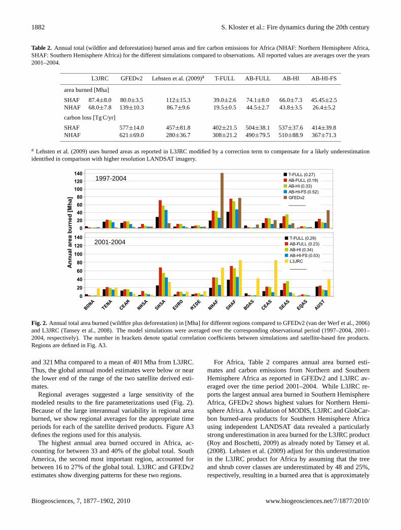
The simulated global (wildfire and deforestation) fire car-bon emissions were between 2.0 and 2.4 Pg C/year for the pe-riod 1997–2004. For the same period GFEDv2 and GICC re-port 2.3 and 2.7 Pg C/year, respectively. For the period 1960to 2000 fire emissions from RETRO are 2.0 Pg C/year. Dur-ing the same period, the simulations ranged between 1.7–2.2 Pg C/year. This suggests that the models yielded reason-able global estimates of carbon emissions over this time pe-riod. Similar to the area burned, the best spatial correlationbetween simulated fire carbon emissions and fire productswas found for the AB-HI-FS simulation (Fig.4).
While we found a large range of annual burned area inour different simulations, the total global carbon emissionswere relatively similar. This non-linear relationship betweenburned area and fire carbon emissions was partly explained
by different aboveground vegetation pools in steady statefor the different simulations (Table3). The different an-nual burned area simulated with the various model config-urations had a large effect on the modeled carbon stock atsteady state. A simulation with high annual area burned (e.g.AB-FULL) had relatively low aboveground biomass carbonpools at steady state and thus lower fuel loads and carbonemissions per unit area burned. In contrast, a simulationwith a low annual area burned (e.g. T-FULL) had relativelyhigh aboveground biomass carbon pools at steady state andthus high rates of fire emissions per unit of burned area. Inaddition, different assumptions about fire-induced mortalityand combustion completeness in the two different fire algo-rithms applied here (see AppendixA3) led to different levelsof fuel consumption. Also, different distributions of burnedarea contribute to different levels of global emissions becauseof the decoupling of burned area and emissions that occurs ata global scale (van der Werf et al., 2006).
Similar to the simulated area burned, modeled fire car-bon emissions were too low over the African continent(738 to 1099 Tg C/year; GFED: 1190 Tg C/year, GICC:1256 Tg C/year) and too high over South America (711 to908 Tg C/year, GFED: 326 Tg C/year, GICC: 502 Tg C/year).For Africa Table2 compares the simulated values for the pe-riod 2001 to 2004 with GFEDv2 and values given inLehstenet al. (2009). Lehsten et al.(2009) utilized a bias cor-rected L3JRC area burned product for Africa to simulatefire carbon emissions within the LPJ-GUESS model (Smithet al., 2001) in a similar approach as described byvan derWerf et al.(2006). Both area burned and fire carbon emis-sions are higher in Northern Hemisphere Africa comparedto Southern Hemisphere Africa in GFEDv2, in contrast withresults fromLehsten et al.(2009) that show higher levels ofburned area and emissions in Southern Hemisphere Africa.The ratio between annual fire carbon emissions and areaburned is 7.2 Tg C/Mha (NHAF) and 4.5 Tg C/Mha (SHAF)for GFEDv2, which is higher than inLehsten et al.(2009)(4.1 and 3.2 Tg C/Mha, respectively). CLM-CN simulationshad significantly higher ratios. As a result, the simulatedfire carbon emissions were comparable or even exceeded theLehsten et al.(2009) values, even though the annual areaburned was simulated significantly lower.
Deforestation fires were between 141 (AB-FULL) and 204(T-FULL) Tg C/year, or approximately 6–9% of global fireemissions, during the 1990s. This was about 34–42% ofthe total conversion flux related to land use change. In ourmodel the importance of fire in the conversion process de-pended on climate-sensitive fire probabilities defined in Ap-pendixA5. As a consequence, larger contributions were sim-ulated in regions with relatively high fire probabilities suchas Northern Hemisphere Africa (∼70%) and lower contribu-tions were simulated in regions with relatively low fire prob-abilities such as Europe (∼30%).
Biogeosciences, 7, 1877–1902, 2010 www.biogeosciences.net/7/1877/2010/

S. Kloster et al.: Fire dynamics during the 20th century 1885
BONA
TENA
CEAM
NHSA
SHSA
EURO
MIDE
NHAF
SHAF
BOAS
CEAS
SEAS
EQAS
AUST
0
100200
300400
500600
700800 T-FULL (0.41/0.38)
AB-FULL (0.25/0.22)AB-HI (0.35/0.27)AB-HI-FS (0.45/0.39)GFEDv2GICC_______
BONA
TENA
CEAM
NHSA
SHSA
EURO
MIDE
NHAF
SHAF
BOAS
CEAS
SEAS
EQAS
AUST
0
100200
300400
500600
700800 T-FULL (0.33)
AB-FULL (0.23)AB-HI (0.30)AB-HI-FS (0.38)RETRO_______
Car
bo
n E
mis
sio
ns
[T
gC
/yea
r]
1997-2004
1960-2000
Fig. 4. Annual mean total (wildfire plus deforestation) fire carbon emissions in [Tg C/year] for differentregions compared to GFEDv2 (van der Werf et al., 2006), GICC (Mieville et al., 2010), and RETRO(Schultz et al., 2008). The model simulations are averaged over the corresponding observational period(1997–2004 or 1960–2000, respectively). The number in brackets denote global spatial correlation co-efficients between simulations and fire products (for the upper panel the first numbers refers to GFEDv2and the second to GICC). Regions are defined in Fig. fig:regionsA3.
53
Fig. 4. Annual mean total (wildfire plus deforestation) fire carbon emissions in [Tg C/year] for different regions compared to GFEDv2(van der Werf et al., 2006), GICC (Mieville et al., 2010), and RETRO (Schultz et al., 2008). The model simulations are averaged overthe corresponding observational period (1997–2004 or 1960–2000, respectively). The number in brackets denote global spatial correlationcoefficients between simulations and fire products (for the upper panel the first numbers refers to GFEDv2 and the second to GICC). Regionsare defined in Fig.A3.
Boreal North America
1997 1998 1999 2000 2001 2002 2003 2004year
0.0
0.5
1.0
1.5
2.0
2.5
carb
on e
mis
sion
s (n
orm
aliz
ed) Central America
1997 1998 1999 2000 2001 2002 2003 2004year
0
1
2
3
4
carb
on e
mis
sion
s (n
orm
aliz
ed)
Equatorial Asia
1997 1998 1999 2000 2001 2002 2003 2004year
0
1
2
3
4
5
carb
on e
mis
sion
s (n
orm
aliz
ed) Global
1997 1998 1999 2000 2001 2002 2003 2004year
0.8
1.0
1.2
1.4
carb
on e
mis
sion
s (n
orm
aliz
ed)
Fig. 5. Annual mean total (wildfire and deforestation) fire carbon emissions normalized by the meanfor 1997–2004 for regions characterized by a high interannual variability reported in the satellite-basedproducts and globally. Solid lines represent model simulations: black: T-FULL, red: AB-FULL, green:AB-HI; blue: AB-HI-FS. Dashed lines are observations: brown: GFEDv2 (van der Werf et al., 2006);orange: GICC (Mieville et al., 2010). Correlation coefficients for the interannual variability for differentregions are given in Table 4.
54
Fig. 5. Annual mean total (wildfire and deforestation) fire carbon emissions normalized by the mean for 1997–2004 for regions characterizedby a high interannual variability reported in the satellite-based products and globally. Solid lines represent model simulations: black: T-FULL, red: AB-FULL, green: AB-HI; blue: AB-HI-FS. Dashed lines are observations: brown: GFEDv2 (van der Werf et al., 2006); orange:GICC (Mieville et al., 2010). Correlation coefficients for the interannual variability for different regions are given in Table4.
4.2 Interannual and seasonal variability
Figure5 shows the interannual variability in total (wildfireand deforestation) fire carbon emissions as simulated be-
tween 1997 and 2004 compared to estimates reported byGFEDv2 (van der Werf et al., 2006) and GICC (Mievilleet al., 2010) for selected world regions, that are character-ized by a high interannual variability (Table4). Correlations
www.biogeosciences.net/7/1877/2010/ Biogeosciences, 7, 1877–1902, 2010

1886 S. Kloster et al.: Fire dynamics during the 20th century
Table 4. Correlation coefficient for the interannual variability (1997–2004) between model simulations and GFEDv2 (van der Werf et al.,2006) and GICC (Mieville et al., 2010) for total (wildfire and deforestation) fire carbon emissions, relative standard deviation (relative sdev)of monthly fire carbon emissions for GFEDv2 or GICC, and the interannual correlation (correlation) between GFEDv2 and GICC. Nonsignificant correlations (confidence level below 90%) are printed in cursive characters. Regions are defined in Fig.A3.
Correlation – interannual variability relative sdev correlation
T-FULL AB-FULL AB-HI AB-HI-FS Observations
region GFEDv2 GICC GFEDv2 GICC GFEDv2 GICC GFEDv2 GICC GFEDv2 GICC GFEDv2/GICC
BONA 0.47 0.26 0.37 0.21 0.32 0.16 0.30 0.12 0.75 0.78 0.93TENA 0.94 0.38 0.94 0.66 0.94 0.64 0.86 0.69 0.37 0.45 0.56CEAM 0.83 0.87 0.81 0.83 0.79 0.82 0.80 0.82 1.17 0.76 0.95NHSA 0.64 0.68 0.89 0.73 0.85 0.80 0.83 0.77 0.64 0.32 0.80SHSA 0.30 0.61 0.18 0.61 0.21 0.63 0.20 0.62 0.31 0.27 0.70EURO 0.48 0.42 0.74 0.68 0.73 0.65 0.80 0.68 0.37 0.35 0.86MIDE −0.03 −0.25 0.36 0.24 0.38 0.28 0.42 0.15 0.57 0.39 0.80NHAF 0.46 0.25 0.39 0.18 0.30 0.14 0.24 0.17 0.12 0.28 −0.02SHAF 0.36 0.56 0.01 0.30 −0.12 0.22 −0.01 0.23 0.12 0.15 0.83BOAS 0.40 0.36 0.29 0.36 0.31 0.38 0.40 0.45 0.70 0.70 0.81CEAS −0.12 0.01 −0.19 0.21 −0.27 0.10 −0.21 0.09 0.17 0.30 0.66SEAS −0.03 −0.22 0.58 0.37 0.56 0.37 0.54 0.32 0.63 0.36 0.94EQAS 0.95 0.99 1.00 0.99 1.00 1.00 1.00 1.00 1.34 1.14 0.98AUST 0.21 0.15 0.09 −0.03 −0.11 −0.17 −0.12 −0.17 0.24 0.27 0.80
GLOB 0.88 0.29 0.92 0.37 0.91 0.37 0.91 0.35 0.14 0.10 0.64
between simulations and GFEDv2 and GICC for all worldregions are listed in Table4.
Considerable interannual variation was observed in re-gions influenced by ENSO. Here the simulations capturedthe enhanced burned area and fire carbon emissions asso-ciated with El Nino induced drought conditions. For ex-ample for equatorial Asia enhanced fire carbon emissionswere simulated in 1997 and to a lesser extent in 2002 inaccordance with GFEDv2 and GICC estimates (with cor-relations of 0.95–1.00). Another peak in emissions oc-curred in 1982/1983 which was consistent with observations(Goldammer and Seibert, 1990; Schultz et al., 2008, data notshown). In Central America fire carbon emissions were high-est during 1998 due to ENSO-induced drought that resultedin catastrophic burning events in the tropical forest of South-ern Mexico and Central America from April to June 1998(Kreidenweis et al., 2001). The models did a poorer jobin reproducing the variability in boreal regions. For exam-ple, the models predicted higher than average emissions inboreal North America during 1998, matching observations(Kasischke and Bruhwiler, 2003), but missed the large burn-ing event in 2004.
The simulation T-FULL underestimated interannual vari-ability and had a lower correlation with GFEDv2 as well asGICC in many regions, including boreal North America, bo-real Asia and Europe. Better results were obtained with theArora and Boer(2005) based algorithm (simulations AB-
FULL, AB-HI, and AB-HI-FS). The explicit treatment of hu-man ignition and fire suppression had only a small impacton the interannual variability between 1997 and 2004, whichwas mainly controled by interannual changes in soil moisturelevels.
The timing of maximum monthly total (wildfire and de-forestation) fire carbon emissions is shown in Fig.6 com-pared to values reported in GFEDv2 (van der Werf et al.,2006), GICC (Mieville et al., 2010) and RETRO (Schultzet al., 2008). The simulated peaks in monthly mean total car-bon emissions occurred in the northern high latitude regionsin July and August in agreement with the satellite-based fireproducts. For the western US the model using theArora andBoer(2005) algorithm had highest emissions during July andAugust. This was consistent with results based on a compre-hensive data compilation of observed burned area (Wester-ling et al., 2003). In contrast, peak emissions occured later inthe year (during September and October) when we used theThonicke et al.(2001) fire algorithm. For Central Americaand Southeast Asia the simulations had maximum monthlyvalues around March–April which also corresponded to thesatellite-based fire products. For the African continent, emis-sions from high fire regions of the Northern Hemisphere (0–10 ◦ N) had a maximum in February–March. Here GFEDv2and RETRO show an earlier peak around December–January,whereas the ATSR-based GICC product peaks mainly aroundFebruary. An analysis of the individual driving factors used
Biogeosciences, 7, 1877–1902, 2010 www.biogeosciences.net/7/1877/2010/

S. Kloster et al.: Fire dynamics during the 20th century 1887
in the Arora and Boer(2005) algorithm (moisture, biomassand ignition probability) revealed that the seasonality in thesimulated fire carbon emissions was largely controlled by themoisture probability (Pm, see also Eq.A7, not shown).
5 20th century trends of fire carbon emissions
We performed a set of sensitivity experiments to disentan-gle the importance of individual external forcing factors: cli-mate, population density, land use change, and wood harvest.Before we present the long-term trends in Sect.5.2 a moredetailed analysis of the sensitivity experiments is given inthe following Sect.5.1.
5.1 Sensitivity to external forcing
The sensitivity studies were solely performed with CLM-CNusing the fire algorithm based onArora and Boer(2005), be-cause this version of the model had the best agreement withcontemporary satellite-based burned area estimates. Thefire-carbon system in the model was highly non-linear andtherefore the individual sensitivities we present here are notadditive. Also, we did not perform sensitivity experiments toevaluate the impact of changing CO2 concentration or nitro-gen deposition on fire carbon emissions.
5.1.1 Climate
To demonstrate the sensitivity of simulated burned area andtotal (wildfire and deforestation) fire carbon emissions tochanges in climate we performed one simulation (AB-CLIM)in which CLM-CN was forced for the years 1973–2004with the NCEP-NCAR 25 year repeat cycle (1942–1972).This simulation served as a control simulation for the AB-FULL simulation, which was forced from 1973 onwards withNCEP-NCAR reanalysis data from 1973 to 2004.
Figure7shows the simulated differences averaged over theperiod 1973–1997 in annual burned area and fire emissionstogether with the changes in the driving factors, precipita-tion and temperature, as well as with the biomass probabil-ity and moisture probability as used in theArora and Boer(2005) fire algorithm (Pb andPm, see Eqs.A6 andA7, re-spectively). Land surface temperatures averaged over 1973–1997 were higher than the 1948–1972 mean in most regions.The global annual mean land surface temperature increasedby 0.3◦C. Precipitation changes were much more hetero-geneous, with large decreases in precipitation over CentralAfrica and Southeast Asia and increases over the USA andparts of South America. Annual burned area responded to thechanges in climate with the largest increase occurring overCentral Africa and parts of Southern Europe and decreasesoccurring in South America, temperate North America andSoutheast Asia. Global annual mean burned area increasedby 4 Mha (∼2%), and total fire carbon emissions by less than1%. Changes in emissions were similar to the area burned
response pattern. Annual burned area increased over Cen-tral Africa and Southern Europe as a direct response to de-creases in precipitation and an enhanced probability of burn-ing based on fuel moisture levels. Increases in soil moistureled to a decrease in the burned area in South America and inthe eastern US. However, small regions along the US WestCoast had a higher annual burned area despite increases insoil moisture. This increase in burned area was explained byan increase in biomass available for burning.
5.1.2 Population density
Besides lightning, humans constitute an important ignitionsource (Robin et al., 2006), but also actively suppress firesin more densely populated areas in which high property val-ues are typically at risk (Stocks et al., 2003; Theobald andRomme, 2007). Human ignition as well as active fire sup-pression largely depend on cultural, economic, and other fac-tors. The dynamics of these interactions with respect to wild-land fire are difficult to quantify and predict at regional toglobal scales (Bowman et al., 2009; Guyette et al., 2002). Inthis study we made an attempt to parametrize the human ig-nition and fire suppression probabilities as a function of pop-ulation density. Details on our approach can be found in theAppendixA4.
Figure8a shows the difference in total (wildfire and defor-estation) fire carbon emissions caused by changing popula-tion density from 1850 onwards together with the populationdensity (Fig.8b) for important source regions (Africa, SouthAmerica, equatorial Asia) and globally. When we did notaccount for fire suppression, increases in population densitycaused an increase in global fire emissions by approximately30% in the 1990s. All world regions showed an increase,which was most pronounced in Southern Hemisphere SouthAmerica (100%) and equatorial Asia (70%). Little impactwas observed for Europe (8%) or boreal Asia (5%).
In contrast, including fire suppression caused almost nochange in global fire emissions, but did change regional dis-tributions. Regions such as Europe, Central Asia, South-east Asia and Middle East had strong decreases in fire emis-sions (−30, −31, −40, −23% in the 1990s, respectively)as a result of increasing urbanization and our assumption ofstronger fire suppression efforts in densely populated areas.In other regions with lower population densities, increasesin population increased the probability of ignitions and firecarbon emissions, including, for example in Southern Hemi-sphere South America, boreal North America and Australia(+15, +10, +20% in the 1990s, respectively). Overall thisled to a better agreement between the spatial pattern of emis-sions in the model and the satellite-based fire products ascompared to the simulations that assumed a constant humanignition probability (AB-FULL) or only accounted for hu-man ignition as a function of population density and not firesuppression (AB-HI), as discussed in Sect.4.1and Fig.4.
www.biogeosciences.net/7/1877/2010/ Biogeosciences, 7, 1877–1902, 2010

1888 S. Kloster et al.: Fire dynamics during the 20th century
T-FULL AB-HI-FS GFEDv2 GICC
JAN FEB MAR APR MAY JUN JUL AUG SEP OCT NOV DEC
JAN FEB MAR APR MAY JUN JUL AUG SEP OCT NOV DEC
JAN FEB MAR APR MAY JUN JUL AUG SEP OCT NOV DEC
JAN FEB MAR APR MAY JUN JUL AUG SEP OCT NOV DECT-FULL AB-HI-FS RETRO
JAN FEB MAR APR MAY JUN JUL AUG SEP OCT NOV DEC
JAN FEB MAR APR MAY JUN JUL AUG SEP OCT NOV DEC
JAN FEB MAR APR MAY JUN JUL AUG SEP OCT NOV DEC
JAN FEB MAR APR MAY JUN JUL AUG SEP OCT NOV DEC
Fig. 6. Month of maximum total (wildfire plus deforestation) fire carbon emissions for the different sim-ulations compared to different fire products: GFEDv2 (van der Werf et al., 2006), GICC (Mieville et al.,2010) and RETRO (Schultz et al., 2008). The model simulations are averaged over the correspondingobservational periods (GFEDv2, GICC: 1997–2004; RETRO: 1960–2000).
55
Fig. 6. Month of maximum total (wildfire plus deforestation) fire carbon emissions for the different simulations compared to different fireproducts: GFEDv2 (van der Werf et al., 2006), GICC (Mieville et al., 2010) and RETRO (Schultz et al., 2008). The model simulations areaveraged over the corresponding observational periods (GFEDv2, GICC: 1997–2004; RETRO: 1960–2000).
precipitation area burned carbon emissions
-10.0 -2.0 -0.5 -0.1 0.0 0.1 0.5 2.0 10.0 -10.0 -2.0 -0.5 -0.1 0.0 0.1 0.5 2.0 10.0 -100 -20 -5 -1 0 1 5 20 100
temperature biomass probability moisture probability
-10.00 -2.00 -0.50 -0.10 0.00 0.10 0.50 2.00 10.00 -100 -20 -5 -1 0 1 5 20 100 -100 -20 -5 -1 0 1 5 20 100
Fig. 7. Difference between simulation AB-FULL and AB-CLIM in annual mean temperature [K], annual mean precipitation [mm/d], annualtotal area burned [% of grid box], annual mean carbon emissions [g C/m2/year] and biomass and moisture probability [×100] as defined inSect.A2 averaged over the period 1973–1997.
Biogeosciences, 7, 1877–1902, 2010 www.biogeosciences.net/7/1877/2010/

S. Kloster et al.: Fire dynamics during the 20th century 1889
Africa
-100
-50
0
50
100
150
200
delta
car
bon
emi [
TgC
/yea
r]
HIHI-FS
South America
0
50
100
150
200
250HIHI-FS
Equatorial Asia
0
50
100
150 HIHI-FS
Global
0
200
400
600HIHI-FS
0.1
0.2
0.3
0.4
0.5
0.6
pop.
den
s. [i
nh./k
m**
2]
0.05
0.10
0.15
0.20
0.25
0.30
0.02
0.04
0.06
0.08
0.10
0.12
0.14
2
3
4
5
1860 1880 1900 1920 1940 1960 1980 2000year
-150
-100
-50
0
delta
car
bon
emi.
[TgC
/yea
r]
TOTALWILDFIRE
1860 1880 1900 1920 1940 1960 1980 2000year
-80
-60
-40
-20
0
TOTALWILDFIRE
1860 1880 1900 1920 1940 1960 1980 2000year
-60
-40
-20
0
TOTALWILDFIRE
1860 1880 1900 1920 1940 1960 1980 2000year
-500
-400
-300
-200
-100
0
TOTALWILDFIRE
Fig. 8. Sensitivity to changes in population density and land use change and wood harvest for selected regions and globally.(A) Annualmean change in carbon emission from total fires (natural and deforestation) caused by changes in population density in the case of onlyhuman ignition is considered (green line, AB-HI – AB-HI-PI) and human ignition and fire suppression considered (blue line, AB-HI-FS –AB-HI-FS-PI) in [Tg C/year];(B) population density [inhabitants/km2]; (C) change in total (wildfire and deforestation) fire carbon emissions(black) and wildfire fire carbon emissions (red) caused by land use change and wood harvest in [Tg C/year] (AB-FULL – AB-LUC).
5.1.3 Land use change and wood harvest
Land use change and wood harvest impact fire carbon emis-sions by introducing a fire source (deforestation fires, whichare frequently used to eliminate biomass in preparation foragricultural use) and by removing biomass available forburning. Thus, the net effect of land use activities can in-crease or decrease fire emissions.
The globally averaged trends in fire emissions from de-forestation showed a large increase over the 20th century(Fig. 9). During the 1990s, the regions that contributed themost to deforestation fire emissions were Asia, Africa andSouth America. Maximum deforestation fires for the 20thcentury occurred in the model during the 1950s and weredriven by large land cover changes globally. At the begin-ning of the 20th century North America, Asia, and Europewere the main contributors to the global deforestation fireflux and Africa and South America were only of minor im-portance.
Globally the deforestation fire carbon loss in the 1990swas 141 Tg C/year. However, adding in deforestation andwood harvest reduced the carbon loss from wildfires by433 Tg C/year (−16%, Fig.8c). This decrease can be ex-plained by a globally reduced aboveground biomass poolcaused by land use change and wood harvest. Global total(wildfire and deforestation) fire emissions were consequentlyreduced by 292 Tg C/year (−11%, Fig.8c).
Regionally, the reduction in total carbon fire emissionswas strongest in boreal North America (−21% in the 1960s),temperate North America (−30% in the 1980s), Europe(−25% in the 1990s) and Southeast Asia (−25% in the
1990s). A few regions and time periods had significantlyenhanced total fire carbon emissions, i.e. deforestation firecarbon emissions more than compensated for any decreasesin wildfire emissions caused by reduced biomass availabil-ity. These regions include: boreal North America (1850sto 1920s: 11–44%), temperate North America (1850s to1890s: 6–15%), Europe (1850s to 1910: 4–11%), borealAsia (1850s to 1990s: 8–100%), central East Asia (1850sto 1980s: 2–27%) and equatorial Asia (1990s: 13%).
Land use change and wood harvest overall led to a 24 Pg Creduction in carbon emitted by wildfires between 1850 and2000, which was partly compensated by deforestation firecarbon emissions of 14 Pg C. Wood harvest accumulated75 Pg C within the same time period, with this carbon ulti-mately redistributed in wood and paper products. 21 Pg Cwere gained by the wood and paper product pools throughland use change and 42 Pg C were lost to the atmosphere bydirect conversion.
Overall land use change activities caused a net terres-trial carbon source of 1.2 Pg C/year in the 1990s. Thisflux is in the range of current estimates ranging between−0.6 Pg C/year and 1.8 Pg C/year (Ito et al., 2008) and sim-ilar to a recent estimate of 1.1 to 1.3 Pg C/year byShevli-akova et al.(2009). During 2000–2004 this source decreasedto 0.85 Pg C/year. Deforestation fires contributed to approxi-mately 11% of this net carbon source.
5.2 Trends in carbon emissions
Mieville et al. (2010) use historical burned area estimates byMouillot et al. (2006) to scale contemporary satellite-based
www.biogeosciences.net/7/1877/2010/ Biogeosciences, 7, 1877–1902, 2010

1890 S. Kloster et al.: Fire dynamics during the 20th century
1860 1880 1900 1920 1940 1960 1980 2000year
0
50
100
150
200
Car
bon
emis
sion
s [T
gC/y
ear]
Middle East+ Australia+ Europe+ North America+ Africa+ South Central America+ Asia = Global
Fig. 9. Annual mean fire emissions from deforestation [Tg C/year] as simulated in simulation AB-FULL. The contribution of each region is stacked onto the region plotted below, so that the black linerepresents the global deforestation carbon loss.
58
Fig. 9. Annual mean fire emissions from deforestation [Tg C/year]as simulated in simulation AB-FULL. The contribution of each re-gion is stacked onto the region plotted below, so that the black linerepresents the global sum of fire emissions from deforestation.
observations back in time (GICChist).Mouillot et al. (2006)note that for the fire history of the 20th century the underly-ing data source is too sparse to support a reconstruction withhigh quantitative accuracy and thus they recommend usingtheir time series to identify large-scale trends and patterns.Here we compared our simulated values against GICChistnormalized to the mean state 1900–2000 in Fig.10, whichalso summarizes the results from the sensitivity experimentsas percentage changes in decadal mean emissions caused bythe individual forcing factors (as described in Sect.5.1).
The trend analysis of our simulation for the 20th centurywas limited as we only forced the model with reanalysisdata corresponding to the 1948–2004 period (before 1948the model was forced with a repeating set of 25 years ofNCEP/NCAR reanalysis from 1948–1972). Changes in to-tal fire carbon emissions before 1948 were therefore onlydriven by changes in the external forcing factors: popula-tion density, atmospheric CO2 concentration, nitrogen depo-sition, land use change, and wood harvest. During 1948–2004 the simulated trends were caused by the full set of ex-ternal forcings including climate.
Globally we found a slight downward trend from 1900 to1960 in agreement with GICChist, except for the simulationthat assumed that human ignition increases with populationdensity, which led to a moderate upward trend. The last threedecades for all simulations were characterized by an upwardtrend caused by climate variations and large burning eventsin 1997–1998 associated with ENSO-induced drought.
GICChist shows a decreasing trend over the 20th cen-tury in boreal regions and an exponential increase in tropicalforests, which the authors relate to more stringent fire sup-
pression policies in boreal regions and the use of fire in de-forestation in the tropical regions, respectively. Near the endof the 20th century, they find some evidence of an increasein burned area within temperate forests.
Our simulated trend was consistent with these findings forthe boreal zone of North America, although our simulatedincrease started slightly later. In particular, land use changeled to deforestation fires between 1900 and 1925 and an in-crease in total fire carbon emissions. Between 1950–1975,however, sustained levels of wood harvesting caused a re-duction in available biomass and a corresponding decrease intotal fire carbon emissions. The magnitude of the simulateddecrease between 1950 and 1975 was much smaller than theone reported in GICChist. A subsequent increase in the mod-eled carbon emissions from 1975 to 2000 was mainly relatedto a combination of land use change activities and climatewarming. In contrast with the AB simulations fire emissionsfrom T-FULL did not change substantially in the boreal re-gions during the 20th century.
For South America GICChist shows an increase through-out the 20th century, which is most pronounced in the lastthree decades. The simulations rather showed a large decadalvariability in fire carbon emissions, due to variations in the25 year cyclic climate forcing through the 1960s, followedby a sharp decrease caused by enhanced precipitation ratesin the 1970s. After the 1970s fire emissions returned to highvalues.
For Europe our simulations were in qualitative agreementwith GICChist, but the simulated trends were smaller. Thebest agreement was achieved by the inclusion of fire sup-pression. In contrast, in Southeast Asia the inclusion of firesuppression caused a pronounced decrease in simulated totalfire carbon emissions throughout the 20th century, which isnot observed in GICChist.
Africa had a pronounced upward trend in total fire carbonemissions for the last decades in the 20th century in the sim-ulations as well as in the trend reported by GICChist. In thesimulations this trend can be explained by a change in cli-mate leading to drier conditions over Northern HemisphereAfrica at the end of the 20th century.
These results are in contrast to those reported byIto andPenner(2005). Ito and Penner(2005) constructed an inven-tory of biomass burning black carbon (BC) and particulateorganic matter (POM) emissions for the period 1870–2000based on a bottom up inventory for open vegetation burningscaled by a top-down estimate for the year 2000. Monthlyand interannual variations were derived from TOMS aerosolindex between 1979 and 2000. Prior to 1979, emissionswere scaled to a CH4 emission inventory based on land usechange (Stern and Kaufmann, 1996). As a result of increas-ing deforestation rates (Houghton et al., 1983) open vege-tation burning increases between 1870 and 2000 in theItoand Penner(2005) estimates. This is in contrast to our sim-ulated decreasing trend in global fire carbon emissions be-tween the 1900s and 1960s caused by strong wood harvesting
Biogeosciences, 7, 1877–1902, 2010 www.biogeosciences.net/7/1877/2010/

S. Kloster et al.: Fire dynamics during the 20th century 1891
Global
0.9
1.0
1.1
carb
on e
mi.
Temperate North America
0.5
1.0
1.5
2.0
2.5Boreal North America
0.5
1.0
1.5
2.0
2.5
1920 1940 1960 1980year
-10
0
10
20
delta
car
bon
emi [
%]
1920 1940 1960 1980year
-20
-10
0
10
20
1920 1940 1960 1980year
-20
-10
0
10
20
30
Europe
0.8
1.0
1.2
1.4
1.6
carb
on e
mi (
norm
aliz
ed)
Middle East
0.8
1.0
1.2
Boreal Asia
1.0
1.5
2.0
1920 1940 1960 1980year
-20
0
20
40
delta
car
bon
emi [
%]
1920 1940 1960 1980year
-30
-20
-10
0
10
20
1920 1940 1960 1980year
0
20
40
60
80
100
120
Fig. 10. Upper panels: Trend in decadal total (wildfire and deforestation) fire carbon emissions com-pared to decadal mean GICChist estimates (Mieville et al., 2010) for different regions from 1900 to2000 normalized with the mean value for 1900–2000. Solid lines represent model simulations: black:T-FULL, red: AB-FULL, green: AB-HI; blue: AB-HI-FS. Dashed orange line with symbols are obser-vations (GICChist); Lower panels: decadal mean change in total carbon loss in [%] with respect to therespective control simulation caused by red: land use change and wood harvest, green: human ignition,blue: human ignition and fire suppression, black: climate. Note here, that the fire carbon-system ishighly non-linear and therefore the individual responses are not additive.
59
Fig. 10.Upper panels: Trend in decadal total (wildfire and deforestation) fire carbon emissions compared to decadal mean GICChist estimates(Mieville et al., 2010) for different regions from 1900 to 2000 normalized with the mean value for 1900–2000. Solid lines represent modelsimulations: black: T-FULL, red: AB-FULL, green: AB-HI; blue: AB-HI-FS. Dashed orange line with symbols are observations (GICChist);Lower panels: decadal mean change in total carbon loss in [%] with respect to the respective control simulation caused by red: land usechange and wood harvest, green: human ignition, blue: human ignition and fire suppression, black: climate. Note here, that the fire carbon-system is highly non-linear and therefore the individual responses are not additive.
rates and decreases in biomass available for burning.Marlonet al.(2008) compiled sedimentary charcoal records over thelast two millennia. Their analysis shows a long-term down-ward trend in biomass burning between 1–1750 followed bya sharp increase from 1750 to the late 19th century and a de-crease from the late 19th to mid-to-late 20th century on theglobal scale. They hypothesize that the long-term downwardtrend following 1870 can be explained by land use changeand wood harvest, which they argue results in landscape frag-mentation and generally less flammable landscapes in manyregions. This is qualitatively consistent with our results.
Schultz et al.(2008) utilize different satellite products forcontemporary fire carbon emissions estimates and an exten-sive literature review in combination with a numerical firemodel to scale these back in time for the time period 1960–
2000. In Fig.11 we compare annual total carbon emis-sions from our simulations to these values. The comparisonshowed in general a reasonable agreement. Our simulationshad a moderate upward trend in total fire carbon emissionsbetween 1970–2000, which was in broad agreement with theRETRO time series and was mainly caused by large burn-ing events in 1982–1983 and 1997–1998 associated with theENSO-induced drought conditions. From 1960 to 1970 thesimulations had a downward trend, whereas RETRO showsalmost no trend. The simulated trends were driven mainlyby changes in climate. Other external forcings such as pop-ulation density, land use change and wood harvest impactedonly slightly the total carbon emissions between 1960 and2000 (cf. Fig.8). Our simulations were qualitatively consis-tent with the findings fromDuncan et al.(2003) that show
www.biogeosciences.net/7/1877/2010/ Biogeosciences, 7, 1877–1902, 2010

1892 S. Kloster et al.: Fire dynamics during the 20th century
South America
0.8
1.0
1.2
1.4
carb
on e
mi (
norm
aliz
ed)
Africa
0.9
1.0
1.1
1.2
1.3
Central Asia
0.8
0.9
1.0
1.1
1.2
1.3
1.4
1920 1940 1960 1980year
-20
-10
0
10
20
30
delta
car
bon
emi [
%]
1920 1940 1960 1980year
-10
0
10
20
30
1920 1940 1960 1980year
-10
0
10
20
Equatorial Asia
1.0
1.5
2.0
carb
on e
mi (
norm
aliz
ed)
South East Asia
0.8
0.9
1.0
1.1
1.2
1.3
Australia
0.8
0.9
1.0
1.1
1.2
1920 1940 1960 1980year
-10
0
10
20
30
40
50
delta
car
bon
emi [
%]
1920 1940 1960 1980year
-30
-20
-10
0
10
20
1920 1940 1960 1980year
-10
0
10
20
30
Fig. 10. Continued.
60
Fig. 10. Continued.
an upward trend in fire emissions between 1979 and 2000,related to large burning events in 1997–1998. TheDuncanet al. (2003) estimates are based on ATSR and AVHRR forseasonal variations and TOMS aerosol index as a surrogatefor interannual variability.
6 Discussion and conclusions
In this study we improved the representation of fire processeswithin the Community Land Model (CLM-CN,Thorntonet al., 2007) and simulated carbon emissions from fires dur-ing the 20th century. CLM-CN originally included a prog-nostic treatment of fires based on the work byThonicke et al.(2001). Here we developed a new fire algorithm based on thework by Arora and Boer(2005). Our goal was to reproducecontemporary observed burned areas and fire carbon emis-sions. For this purpose we extended the model by an ex-plicit treatment of the human ignition and fire suppression asa function of population density. In addition, we introduceda parametrization of deforestation fire carbon emissions mak-
ing use of land use change transition scenarios (Hurtt et al.,2006). We performed several sensitivity experiments to sepa-rate the effects of external driving factors (population density,land use change and wood harvest, and climate) on fire emis-sions over the last century. The results of this study providea self-consistent emissions dataset for fire emissions of car-bon dioxide, reactive gases and aerosols for the 20th century(not discussed here), which can be used in future in chemicaltransport and climate modeling studies.
Our model was able to capture much of the observed meanand variability in burned area and carbon emissions. Sim-ulated global annual total fire carbon emissions ranged be-tween 2.0 and 2.4 Pg C/year for the time period 1997 to 2004and were within the uncertainty of satellite-based estimates.For the most part the model captured the observed patterns offires, but we consistently overestimated annual area burnedand emissions for South America and underestimated thesequantities for Africa when we compared our simulations toa range of observations. This mismatch could be the re-sult of several factors including an overestimation of the
Biogeosciences, 7, 1877–1902, 2010 www.biogeosciences.net/7/1877/2010/

S. Kloster et al.: Fire dynamics during the 20th century 1893
Global
1960 1970 1980 1990 2000year
1.5
2.0
2.5
3.0
3.5
Car
bon
emis
sion
s [P
gC/y
ear]
T-FULLAB-FULLAB-HIAB-HI-FSRETRO
Fig. 11. Annual mean total (wildfire and deforestation) fire carbon emissions in [Pg C/year] for thedifferent simulations from 1960–2000 compared to values reported in RETRO (Schultz et al., 2008).
61
Fig. 11. Annual mean total (wildfire and deforestation) fire carbonemissions for the different simulations from 1960–2000 comparedto values reported in RETRO (Schultz et al., 2008).
live aboveground biomass in the Amazon basin in CLM-CN(Randerson et al., 2009). On interannual timescales we founda reasonably good agreement between simulated fire emis-sions and satellite-based results. All simulations captured thelarge interannual variability associated with El-Nino-induceddrought conditions in equatorial Asia. Our model was ableto predict the timing of peak emissions in many parts of theworld. However, for Central Africa our simulations tendedto simulate the timing of maximum monthly emissions dur-ing February/March, lagging the observations by one to twomonths. TheArora and Boer(2005) fire algorithm extendedby a parametrization of human ignition and fire suppressionprovided the best agreement with the observations in term ofspatial pattern, interannual and seasonal variability and long-term trends during the 20th century.
To improve the fire model, and generally our understand-ing of fires in the Earth System, we require improved data ona global scale. Large discrepancies remain between the dif-ferent satellite sensor products (Boschetti et al., 2004; Royand Boschetti, 2009; Chang and Song, 2009; Giglio et al.,2010), which hampers prognostic model validation in manyregions. Improved satellite fire products that include un-certainty ranges would facilitate development of improvedglobal prognostic fire algorithms. Also, estimates of defor-estation fire carbon emissions are associated with large un-certainties. In our model they depend strongly on the as-sumptions made in the underlying land use change scenario,wood harvesting rates and the apportionment of carbon af-fected by land use change into product and conversion pools.In addition, the breakdown of the conversion flux into fire
and non-fire related carbon emissions using ratios that solelydepend on the moisture driven fire probability, as done in thisstudy, does not account for cultural and socio-economic fac-tors that often control deforestation fire emissions (Mortonet al., 2006; Geist, 2001). Satellite-based estimates on forestclearing (Hansen et al., 2008) combined with satellite-basedfire products should improve our understanding of deforesta-tion fires in the future and will help to further improve thedeforestation fire parametrization introduced in this study.In addition, there are many important processes related tofires that are not included in the fire algorithms used in thisstudy such as maintenance fires (van der Werf et al., 2009),seasonal changes in combustion factors due to varying fuelmoisture and litter amounts (Hoffa et al., 1999), and peatfires (Page et al., 2002). Also, a more detailed analysis ofthe relationship between population distribution and humanignition and fire suppression is an important task to reduceuncertainties in the modeling of fires.
Using our improved model we predicted the following pat-terns of fire emissions during the 20th century:
– The simulations had a small global downward trend indecadal mean fire carbon emissions between 1900 and1960 (∼−5%). This downward trend in many regionswas explained by land use change and wood harvest andan associated decrease in available biomass.
– The last three decades in the 20th century were dom-inated by an upward trend in global total fire carbonemissions (∼+30%) caused by climate variations andlarge burning events associated with ENSO-induceddrought conditions.
– Land use change activities between 1850 and 2000 re-leased 14 Pg C from deforestation fires, but reduced car-bon emissions from wildfires by 24 Pg C. Thus, total(wildfire and deforestation) fire carbon emissions werereduced by 10 Pg C (−3%).
– The net flux of carbon to the atmosphere due to landuse activities was simulated as 1.2 Pg C/year for 1990–1999 (similar to previous estimates inIto et al., 2008;Shevliakova et al., 2009). For 2000–2004 this sourcedecreased to 0.85 Pg C/year.
– Deforestation fires contributed to about 6–9% of the to-tal global fire carbon emissions during 1990–1999. Thelargest contribution from these fires (8–15%) occurredduring the 1950s due to strong land use change activitiesglobally.
Our 20th century trends were broadly consistent with esti-mates based on sedimentary charcoal records (Marlon et al.,2008) and historical estimates based on published data,land use practices, qualitative reports and tree ring analysis(Mouillot et al., 2006). However, discrepancies remain on
www.biogeosciences.net/7/1877/2010/ Biogeosciences, 7, 1877–1902, 2010

1894 S. Kloster et al.: Fire dynamics during the 20th century
regional scales and further work is required to resolve thesedifferences.
Although the model was limited in the processes consid-ered and simplified in many aspects, it captured reasonablywell the global distribution and interannual variability. Themodel can be introduced into an Earth System model. Thiswill be an important step towards quantifying the role of firein climate-carbon feedbacks.
Appendix A
Fire algorithms in CLM-CN
Two fire algorithms were implemented into CLM-CN basedon the work byThonicke et al.(2001) andArora and Boer(2005). The fire algorithms have common elements, includ-ing that they first estimate the area burned and then carbonfluxes related to combustion and mortality. WhileThonickeet al. (2001) uses an empirical relationship relating fire sea-son length and burned area,Arora and Boer(2005) intro-duces a process based fire parametrization. Both algorithmsand their implementation into CLM-CN are described morein detail in the following sections.
A1 Fire algorithm based onThonicke et al. (2001)
The fire algorithm developed for the LPJ model (Sitch et al.,2003) was modified byThornton et al.(2007) to translatefrom the original annual time step to the sub-daily time stepused for carbon and nitrogen calculations in CLM-CN. Thealgorithm assumes that fire occurrence is solely a function offuel-availability and inferred fuel moisture conditions. Igni-tion sources are assumed to be ubiquitous and uniform. De-tails on the assumptions made can be found inThonicke et al.(2001). Here we report how the algorithm was implementedinto CLM-CN.
A1.1 Fire probability
A minimum of 100 g C/m2 of dead fuel is required for fireoccurrence. The dead fuel density in CLM-CN is the sumof the litter and coarse woody debris pool. In order to al-low fire occurrence and fire spread the fuel moisture also hasto be below a certain threshold (moisture of extinction,me).The moisture of extinction is assumed to be 0.3 for woodybiomass and 0.2 for herbaceous biomass. As a substitute forfuel moisture, which is not simulated in CLM-CN, the soilmoisture (m) as a fraction of the plant-available volumetricwater content of the top 5 cm of the soil column is used sim-ilar to Thonicke et al.(2001). In addition to fuel availabilityand fuel moisture constraints, fire occurrence is controlled bysurface temperatures, which have to be above freezing.
The probability of fire occurrence at least once a day isgiven as:
fp =
exp
(−π ∗
(mme
)2)
if fuel density> 100 g C/m2,
m <me,
andT > 273.15 K,
0 otherwise.
(A1)
A1.2 Area burned
In Thonicke et al.(2001) the daily fire occurrence probabil-ity is used to estimate the annual mean fire season length(N , [days/yr]), by summing fp over a year, withN updatedonce per year. This approach is modified in CLM-CN.N isupdated every model timestep using an e-folding approxima-tion for the annual sum of fp. This translates the annual timestep fromThonicke et al.(2001) into the sub-daily modeltimestep of CLM-CN to account for seasonal variations infire occurrence.
The e-folding approximation is done as follows: Then-time step running mean of a variablex at the model time stepi (xi) was approximated by the following weighted sum:
xi = xi−1n−1
n+xi
1
n(A2)
For an annual running mean the number of e-foldingtimesteps (n) was set to the number of model time steps ina year.
FollowingThonicke et al.(2001) the annual fractional areaburned (fannual, [fraction burned/yr]) was derived from theone-year e-folding mean fire probability (¯fpi) at each modeltimestepi:
fannual= ¯fpi ·exp
(s−1
0.45(s−1)3+2.83(s−1)2+2.91(s−1)+1.04
)(A3)
with s = N/365. The fractional area burned per time step inseconds1t (f1t ) is given as:
f1t =
{ fpi
Nfannual
1t86400 for N = 365· ¯fpi 6= 0,
0 for N = 365· ¯fpi = 0.(A4)
A2 Fire algorithm based onArora and Boer (2005)
The fire algorithm developed for the CTEM model (Verseghyet al., 1993) is implemented into CLM-CN. Details on thealgorithm are given inArora and Boer(2005). Here we de-scribe how the algorithm was implemented into CLM-CN.
A2.1 Fire probability
Total probability of fire occurrence is estimated as the prod-uct of three scalars that represent control from biomass,moisture and ignition:
P = PbPmPi (A5)
Biogeosciences, 7, 1877–1902, 2010 www.biogeosciences.net/7/1877/2010/

S. Kloster et al.: Fire dynamics during the 20th century 1895
wherePb takes into account that a certain biomass has to beavailable for burning and is represented as:
Pb = max[0,min(1,(F −Fl)/(Fu−Fl))] (A6)
with Fl=200 g C/m2 and Fu=1000 g C/m2 and F is theaboveground biomass available for burning (combined leaf,stem, litter and coarse woody debris (cwd) pools).
Pm is the fire probability conditioned on the moisture (m)and expressed as follows:
Pm = 1− tanh(1.75·m/me)2 (A7)
me is the moisture of extinction, defined here as 0.35 inde-pendent of fuel type. We definedm in the same way as forthe Thonicke et al.(2001) algorithm as a fraction of plant-available volumetric water content in the top 5 cm of the soilas a surrogate for fuel moisture content.
Pi represents the probability of an ignition source,which can be either human or natural (lightning). Ig-nition due to lightning is represented using cloud toground lightning frequency (flashes/km2/month) which islinearly scaled between essentially no flashes (LFlow =
0.02 flashes/km2/month) and the maximum observed values(LFup=0.70 flashes/km2/month).
βi = max[0,min(1,(LF−LFlow)/(LFup−LFlow))] (A8)
For the lightning frequency we used the Lightning Imag-ing Sensor/Optical Transient Detector product (LIS/OTD)which reports total flash rates (cloud-to-ground and intra-cloud flashes). We estimated the fraction of the total flashrate that can ignite a fire (cloud-to-ground flashes) by intro-ducing a latitude dependency of the fraction of total flashesto cloud-to-ground flashes (Pierce, 1969).
The probability of the ignition by lightning is formulatedas follows:
Pl = βi/(βi +exp(1.5−6βi)) (A9)
The total ignition potential (combination of natural ignitionand human potential (Ph)) is formulated according to:
Pi = Pl +(1−Pl)Ph (A10)
A2.2 Area burned
The area burned is assumed to form an elliptical shapearound the point of ignition defined by the fire spread ratesin upwind and downwind directions as well as the length-to-breath ratio of the ellipse. To be in accordance with the dailytime step used inArora and Boer(2005) we applied an e-folding approximation of the daily mean following Eq. (A2).For the area burned calculations we exactly used the formu-lation given byArora and Boer(2005). For completeness wereport them here. For details on the parameters and assump-tions applied we refer the reader toArora and Boer(2005).
The fire spread rate in [km/h] in downwind direction isrepresented as:
up = g(ws)h(m)umax (A11)
with umax the maximum fire spread rate (0.45 km/h). Thedependence on the wind speed (ws) is given by
g(ws) = 1.0−(1.0−g0)exp(−(ws2/2500)) (A12)
In hereg0 is 0.1 and ws is the wind speed in [km/h].The dependence upon the moisture is represented with
h(m)
h(m) = (1−βm)2 (A13)
βm =
{m/me for m <me,
1 for m >me.(A14)
The length to breath ratio is given by:
lb = 1+10(1−exp(−0.017·ws)) (A15)
Assuming that the downwind fire spread rate equals 0.2 theupwind fire spread rate, the total area burned in [km2] is thengiven as:
a = 0.36·π ·u2p/lb · t2 (A16)
Assuming that the fire burns on average one day, the actualpotential area burned within one day can be approximated as:
A = a (1−q)(2−q)/q2 (A17)
with q=0.5. The area affected in a time step is then given asthe product of fire probability (P ), the potential area burned(A) divided by the number of model timesteps within a day(86 400/1t)
Aburn= A ·P ·(1t/86 400) (A18)
This area burned (Aburn) is according toArora and Boer(2005) representative for 1000 km2. The fractional areaburned per time step1t is subsequently given by:
f1t = Aburn/1000. (A19)
A3 Fire emission, combustion completeness andmortality
To account for different levels of mortality associated withfire in different vegetation types and that only part of theaffected biomass is combusted and released into the atmo-sphere, we introduced a mortality factor (mort) and a com-bustion completeness factor (cc) as functions of the differentPFTs and fuel types considered in CLM-CN. Similar factorsare defined byArora and Boer(2005). Thonicke et al.(2001)uses a “fire resistance” factor (1−mort), which varies amongdifferent plant functional types, but does not account for thefact that biomass is only partly combusted during a fire. InCLM-CN we modified theThonicke et al.(2001) algorithm
www.biogeosciences.net/7/1877/2010/ Biogeosciences, 7, 1877–1902, 2010

1896 S. Kloster et al.: Fire dynamics during the 20th century
Table A1. Mortality (MORT) factors for different plant functional types and fuel types afterThonicke et al.(2001) and combustion com-pleteness (CC) factors used in CLM-CN in combination with theThonicke et al.(2001) algorithm.
PFT CC Leaf CC Stem CC Root CC Litter CC CWD MORT Leaf MORT Stem MORT Root
needleleaf evergreen temperate tree 1.0 0.2 0.2 1.0 0.2 0.78 0.78 0.78needleleaf evergreen boreal tree 1.0 0.2 0.2 1.0 0.2 0.78 0.78 0.78needleleaf deciduous boreal tree 1.0 0.2 0.2 1.0 0.2 0.78 0.78 0.78broadleaf evergreen tropical tree 1.0 0.2 0.2 1.0 0.2 0.78 0.78 0.78broadleaf evergreen temperate tree 1.0 0.2 0.2 1.0 0.2 0.50 0.50 0.50broadleaf deciduous tropical tree 1.0 0.2 0.2 1.0 0.2 0.50 0.50 0.50broadleaf deciduous temperate tree 1.0 0.2 0.2 1.0 0.2 0.78 0.78 0.78broadleaf deciduous boreal tree 1.0 0.2 0.2 1.0 0.2 0.78 0.78 0.78broadleaf evergreen shrub 1.0 0.2 0.2 1.0 0.2 0.78 0.78 0.78broadleaf deciduous temperate shrub 1.0 0.2 0.2 1.0 0.2 0.78 0.78 0.78broadleaf deciduous boreal shrub 1.0 0.2 0.2 1.0 0.2 0.78 0.78 0.78c3 arctic grass 1.0 0.2 0.2 1.0 0.2 1.0 1.0 1.0c3 non-arctic grass 1.0 0.2 0.2 1.0 0.2 1.0 1.0 1.0c4 grass 1.0 0.2 0.2 1.0 0.2 1.0 1.0 1.0
Table A2. Combustion Completeness (CC) and Mortality (MORT) factors for different plant functional types and fuel types afterArora andBoer(2005).
PFT CC Leaf CC Stem CC Root CC Litter CC CWD MORT Leaf MORT Stem MORT Root
needleleaf evergreen temperate tree 0.8 0.5 0.0 0.5 0.5 0.9 0.8 0.1needleleaf evergreen boreal tree 0.8 0.5 0.0 0.5 0.5 0.9 0.8 0.1needleleaf deciduous boreal tree 0.8 0.5 0.0 0.5 0.5 0.9 0.8 0.1broadleaf evergreen tropical tree 0.8 0.5 0.0 0.6 0.6 0.9 0.8 0.1broadleaf evergreen temperate tree 0.8 0.5 0.0 0.6 0.6 0.9 0.8 0.1broadleaf deciduous tropical tree 0.8 0.5 0.0 0.6 0.6 0.9 0.6 0.1broadleaf deciduous temperate tree 0.8 0.5 0.0 0.6 0.6 0.9 0.6 0.1broadleaf deciduous boreal tree 0.8 0.5 0.0 0.6 0.6 0.9 0.6 0.1broadleaf evergreen shrub 0.8 0.5 0.0 0.6 0.6 0.9 0.6 0.1broadleaf deciduous temperate shrub 0.8 0.5 0.0 0.6 0.6 0.9 0.8 0.1broadleaf deciduous boreal shrub 0.8 0.5 0.0 0.6 0.6 0.9 0.8 0.1c3 arctic grass 0.9 0.0 0.0 0.7 0.7 0.9 0.0 0.25c3 non-arctic grass 0.9 0.0 0.0 0.7 0.7 0.9 0.0 0.25c4 grass 0.9 0.0 0.0 0.7 0.7 0.9 0.0 0.25
by adding a woody combustion completeness factor (0.2) thatis applied to all woody fuel types. All other fuel types arecompletely combusted.
The amount of carbon released into the atmosphere foreach PFT is given as:
EPFT= f1t ·C ·cc·mort (A20)
with C=(Cleaf,Cstem,Croot,Clitter,Ccwd) being a vector ofcarbon concentrations in [g/m2] for the different fuel typesconsidered in CLM-CN and cc and mort being a vector ofcombustion completeness and mortality factors, respectively,as defined in Tables A1 and A2. The amount of carbon killed
during a fire and transferred to the litter pool for each PFT isgiven as:
TPFT= f1tC(1−cc)mort (A21)
Total carbon emission (Ec) are given as the area weightedsum over all PFTs. The same applies for nitrogen.
A4 Human influence
Humans influence fires by ignition (intentionally or acci-dentally) and at the same time they impact fires actively byfire suppression. To account for these effects we introduceda parametrization of the human ignition potential and firesuppression as a function of population density. Populationdensity data were taken from the HYDE dataset for the years
Biogeosciences, 7, 1877–1902, 2010 www.biogeosciences.net/7/1877/2010/
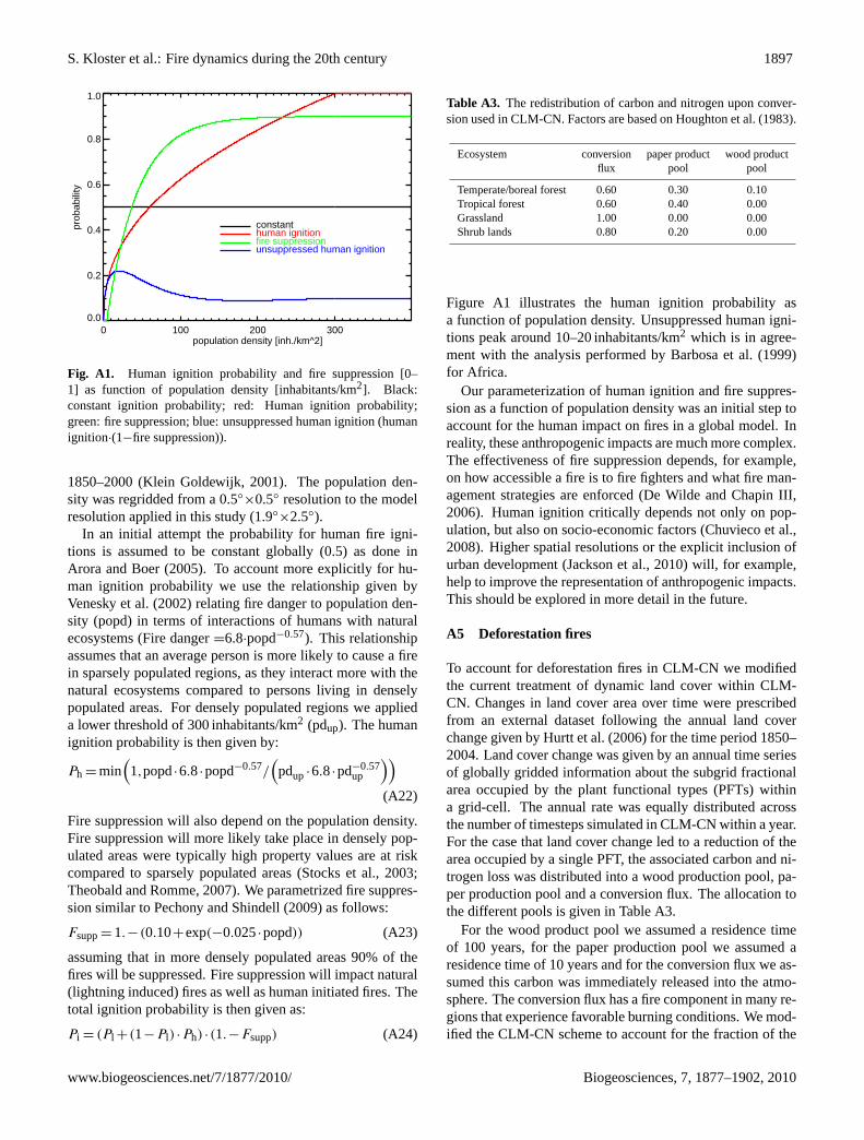
S. Kloster et al.: Fire dynamics during the 20th century 1897
0 100 200 300population density [inh./km^2]
0.0
0.2
0.4
0.6
0.8
1.0
prob
abili
ty
constanthuman ignitionfire suppressionunsuppressed human ignition
Fig. A1. Human ignition probability and fire suppression [0–1] as function of population density[inhabitants/km2]. Black: constant ignition probability; red: Human ignition probability; green: firesuppression; blue: unsuppressed human ignition (human ignition∗(1−fire suppression)).figure
62
Fig. A1. Human ignition probability and fire suppression [0–1] as function of population density [inhabitants/km2]. Black:constant ignition probability; red: Human ignition probability;green: fire suppression; blue: unsuppressed human ignition (humanignition·(1−fire suppression)).
1850–2000 (Klein Goldewijk, 2001). The population den-sity was regridded from a 0.5◦
×0.5◦ resolution to the modelresolution applied in this study (1.9◦
×2.5◦).In an initial attempt the probability for human fire igni-
tions is assumed to be constant globally (0.5) as done inArora and Boer(2005). To account more explicitly for hu-man ignition probability we use the relationship given byVenesky et al.(2002) relating fire danger to population den-sity (popd) in terms of interactions of humans with naturalecosystems (Fire danger=6.8·popd−0.57). This relationshipassumes that an average person is more likely to cause a firein sparsely populated regions, as they interact more with thenatural ecosystems compared to persons living in denselypopulated areas. For densely populated regions we applieda lower threshold of 300 inhabitants/km2 (pdup). The humanignition probability is then given by:
Ph = min(1,popd·6.8·popd−0.57/
(pdup·6.8·pd−0.57
up
))(A22)
Fire suppression will also depend on the population density.Fire suppression will more likely take place in densely pop-ulated areas were typically high property values are at riskcompared to sparsely populated areas (Stocks et al., 2003;Theobald and Romme, 2007). We parametrized fire suppres-sion similar toPechony and Shindell(2009) as follows:
Fsupp= 1.−(0.10+exp(−0.025·popd)) (A23)
assuming that in more densely populated areas 90% of thefires will be suppressed. Fire suppression will impact natural(lightning induced) fires as well as human initiated fires. Thetotal ignition probability is then given as:
Pi = (Pl +(1−Pl) ·Ph) ·(1.−Fsupp) (A24)
Table A3. The redistribution of carbon and nitrogen upon conver-sion used in CLM-CN. Factors are based onHoughton et al.(1983).
Ecosystem conversion paper product wood productflux pool pool
Temperate/boreal forest 0.60 0.30 0.10Tropical forest 0.60 0.40 0.00Grassland 1.00 0.00 0.00Shrub lands 0.80 0.20 0.00
Figure A1 illustrates the human ignition probability asa function of population density. Unsuppressed human igni-tions peak around 10–20 inhabitants/km2 which is in agree-ment with the analysis performed byBarbosa et al.(1999)for Africa.
Our parameterization of human ignition and fire suppres-sion as a function of population density was an initial step toaccount for the human impact on fires in a global model. Inreality, these anthropogenic impacts are much more complex.The effectiveness of fire suppression depends, for example,on how accessible a fire is to fire fighters and what fire man-agement strategies are enforced (De Wilde and Chapin III,2006). Human ignition critically depends not only on pop-ulation, but also on socio-economic factors (Chuvieco et al.,2008). Higher spatial resolutions or the explicit inclusion ofurban development (Jackson et al., 2010) will, for example,help to improve the representation of anthropogenic impacts.This should be explored in more detail in the future.
A5 Deforestation fires
To account for deforestation fires in CLM-CN we modifiedthe current treatment of dynamic land cover within CLM-CN. Changes in land cover area over time were prescribedfrom an external dataset following the annual land coverchange given byHurtt et al.(2006) for the time period 1850–2004. Land cover change was given by an annual time seriesof globally gridded information about the subgrid fractionalarea occupied by the plant functional types (PFTs) withina grid-cell. The annual rate was equally distributed acrossthe number of timesteps simulated in CLM-CN within a year.For the case that land cover change led to a reduction of thearea occupied by a single PFT, the associated carbon and ni-trogen loss was distributed into a wood production pool, pa-per production pool and a conversion flux. The allocation tothe different pools is given in Table A3.
For the wood product pool we assumed a residence timeof 100 years, for the paper production pool we assumed aresidence time of 10 years and for the conversion flux we as-sumed this carbon was immediately released into the atmo-sphere. The conversion flux has a fire component in many re-gions that experience favorable burning conditions. We mod-ified the CLM-CN scheme to account for the fraction of the
www.biogeosciences.net/7/1877/2010/ Biogeosciences, 7, 1877–1902, 2010

1898 S. Kloster et al.: Fire dynamics during the 20th century
1850 - no fire suppression 2000 - no fire suppression
0.0 0.1 0.2 0.3 0.4 0.5 0.6 0.7 0.8 0.9 1.0
0.0 0.1 0.2 0.3 0.4 0.5 0.6 0.7 0.8 0.9 1.01850 - fire suppression 2000 - fire suppression
0.0 0.1 0.2 0.3 0.4 0.5 0.6 0.7 0.8 0.9 1.0
0.0 0.1 0.2 0.3 0.4 0.5 0.6 0.7 0.8 0.9 1.0
0.0 0.1 0.2 0.3 0.4 0.5 0.6 0.7 0.8 0.9 1.0
Fig. A2. Annual mean total ignition probability for the years 1850 and 2000 with and without firesuppression considered.
63
Fig. A2. Annual mean total ignition probability for the years 1850 and 2000 with and without fire suppression considered.
BONATENACEAMNHSASHSAEUROMIDENHAFSHAFBOASCEASSEASEQASAUST
Fig. A3. Map of the 14 regions as defined in van der Werf et al. (2006) used in this study. BONA: BorealNorth America, TENA: Temperate North America, CEAM: Central America, NHSA: Northern Hem.South America, SHSA: Southern Hem. South America, EURO: Europe, MIDE: Middle East, NHAF:Northern Hem. Africa, SHAF: Southern Hem. Africa, BOAS: Boreal Asia, CEAS: Central Asia, SEAS:South East Asia, EQAS: Equatorial Asia, AUST: Australia.
fig:regions64
Fig. A3. Map of the 14 regions as defined invan der Werfet al. (2006) used in this study. BONA: Boreal North Amer-ica, TENA: Temperate North America, CEAM: Central Amer-ica, NHSA: Northern Hem. South America, SHSA: SouthernHem. South America, EURO: Europe, MIDE: Middle East, NHAF:Northern Hem. Africa, SHAF: Southern Hem. Africa, BOAS:Boreal Asia, CEAS: Central Asia, SEAS: Southeast Asia, EQAS:Equatorial Asia, AUST: Australia.
conversion flux that was combusted (deforestation fires) asfollows:
The conversion flux is divided into a fire and non-fire re-lated pool. For this we define a fire-scalar (fs) as a functionof the annual mean fire moisture probability (Pm,annual) sim-ulated within the fire algorithm in CLM-CN (see Eqs.A1 andA7, respectively).
We assume that in regions with a high annual mean firemoisture probability, land managers will more likely burnforest biomass during the land clearing process. The fire-scalar is given as:
fs = fsmin+(max
[0,min
(1,(Pm,annual− fplow)/
(fphigh− fplow))])
·(fsmax−f smin)
In an initial attempt we assumed that the maximum and min-imum fraction of the conversion flux (fsmin) and (fsmax) thatis redirected to the fire and non-fire pool are constant glob-ally (0.2 and 0.8, respectively). However, this ratio will alsolargely depend on cultural practices and is therefore likely tovary for different regions and different time periods.
Low and high annual mean moisture fire probabilities(fplow) and (fphigh) were set to 0.01 and 0.30, respectively.Annual mean moisture fire probabilities are below 0.01 forexample in wet regions like northern Europe and the East
Biogeosciences, 7, 1877–1902, 2010 www.biogeosciences.net/7/1877/2010/

S. Kloster et al.: Fire dynamics during the 20th century 1899
coast of the USA, whereas values larger than 0.30 are sim-ulated only in very dry regions such as Central Africa andAustralia. Annual mean fire moisture probabilities slightlydiffered between the two fire algorithms applied in this study.However, we used the same thresholds for both.
The flux into the fire pool and non-fire pool is given as:
fire poolgain= CONV· fs (A25)
non fire poolgain= CONV·(1− fs) (A26)
with CONV being the carbon and nitrogen mass flux at-tributed to the conversion flux.
The flux out of the fire-pool follows a rate constant, whichis a function of the instantaneous fire moisture probability(Pm,inst) as simulated within the fire algorithm. Carbon in thefire-pool can accumulate over a certain time-period (τmax) inwhich conditions are relatively wet and is only released intothe atmosphere when conditions get sufficiently dry (Mortonet al., 2008; van der Werf et al., 2009). The rate constantwhich controls the flux out of the fire pool is given as:
τfire = τmin+max[0,min(1,(Pm,inst−fi low)/(fihigh−fi low))]
·(τmax−τmin)
τmin andτmax are set to give a 90% loss of the initial massof the fire-pool to be released into the atmosphere within 3years and 1 week, respectively. filow and fihigh are set to 0.0and 1.0. The flux out of the non-fire pool into the atmosphereis immediate (fuel wood).
The flux out of the fire pool and non-fire pool is given as:
fire poolloss= fire pool·τfire (A27)
non fire poolloss= non fire pool·1. (A28)
with fire pool and nonfire pool representing the carbon andnitrogen mass in the fire and non-fire pool, respectively.
In addition to land cover change CLM-CN accounts ex-plicitly for changes in wood harvest activity (Hurtt et al.,2006). Wood harvest is solely related to logging and is notdirectly related to fires. However, wood harvest will alter thebiomass available for burning and thus natural fires as wellas deforestation fires (see Sect.5.1.3).
Acknowledgements.This work was supported by NSF-0758369,NSF-0832782, and NSF-0628353. For computational support theauthors acknowledge the National Science Foundation (NSF) andthe National Center for Atmospheric Research (NCAR). NCAR issponsored by the NSF. We thank the participants and organizersof the AIMES workshop “Cultural Uses and Impacts of Fires” aswell as S. Harrison, K. Thonicke and G. van der Werf for helpfuldiscussion.
Edited by: E. Falge
References
Andreae, M. O., Rosenfeld, D., Artaxo, P., Costa, A. A., Grank,G. P., Longo, K. M., and Silva-Dias, M. A. F.: Smoking RainClouds over the Amazon, Science, 303, 1337–1342, 2004.
Arora, V. K. and Boer, G. J.: Fire as an interactive componentof dynamic vegetation models, J. Geophys. Res., 110, G02008,doi:10.1029/2005JG000042, 2005.
Barbosa, P. M., Stroppiana, D., Gregoire, J.-M., and Pereira,J. M. C.: An assessment of vegetation fire in Africa (1981-1991): Burned areas, burned biomass, and atmospheric emis-sions, Global Biogeochem. Cycles, 13, 933–950, 1999.
Bond, W. J., Woodward, F., and Midgley, G. F.: The global distri-bution of ecosystems in a world without fire, New Phytologist,165, 525–538, doi:10.1111/j.1469-8137.2004.01252.x, 2004.
Boschetti, L., Eva, H. D., Brivio, P. A., and Gregoire, J. M.: Lessonsto be learned form the comparison of three satellite-derivedbiomass burning products, Geophys. Res. Lett., 31, L21501,doi:10.1029/2004GL021229, 2004.
Bowman, D. M. J. S., Balch, J. K., Artaxo, P., Bond, W. J., Carlson,J. M., Cochrane, M. A., D’Antonio, C. M., DeFries, R. S., Doyle,J. C., Harrison, S. P., Johnston, F. H., Keeley, J. E., Krawchuk,M. A., Kull, C. A., Marston, J. B., Mortiz, M. A., Prentice, I. C.,Roos, C. I., Scott, A. C., Swetnam, T. W., van der Werf, G. R.,and Pyne, S. J.: Fire in the Earth System, Science, 324, 481,doi:10.1126/science.1163886, 2009.
Chambers, S. D., Beringer, J., Randerson, J. T., and Chapin III,F. S.: Fire effects on net radiation and energy partitioning: Con-trasting responses of tundra and boreal forest ecosystems, J. Geo-phys. Res., 110, D09106, doi:10.1029/2004JD2005299, 2005.
Chang, D. and Song, Y.: Comparison of L3JRC and MODIS globalburned area products from 2000 to 2007, J. Geophys. Res., 114,D16106, doi:10.1029/2008JD011361, 2009.
Chuvieco, E., Giglio, L., and Justice, C.: Global parameterization offire activity: toward defining fire regimes from Earth observationdata, Glob. Change Biology, 14, 1488–1502, doi:10.1111/j.1365-2486.2008.04585.x, 2008.
Crutzen, P., Heidt, L. E., Krasnec, J. P., Pollock, W. H., andSeiler, W.: Biomass burning as a source of atmospheric gasesCO,H2,N2O,NO,CH3CL and COS, Nature, 282, 253–256,doi:10.1038/282253a0, 1979.
De Wilde, L. and Chapin III, F.: Human impact on the fireregime of interior Alaska: Interactions among fuels, ignitionsources, and fire suppression, Ecosystems, 9, 8, doi:10.1007/s10021-006-0095-0, 2006.
Decker, R. M. and Zeng, X.: Impact of modified richardsequation on global soil moisture simulation in the Commu-nity Land Model (CLM3.5), J. Adv. Model. Earth Syst., 1,doi:10.3894/JAMES.2009.1.5, 2009.
Duncan, B. N., Martin, R. V., Staudt, A. C., Yevich, R., and Logan,J. A.: Interannual and seasonal variability of biomass burningemissions constrained by satellite observations, J. Geophys. Res.,108, D24100, doi:10.1029/2002JD002378, 2003.
Feingold, G., Remer, L. A., Ramaprasad, J., and Kaufman, Y. J.:Analysis of smoke impact on clouds in Brazilian biomass burn-ing regions: An extension of Twomey’s approach, J. Geophys.Res., 103, 22907–22922, 2001.
Flanner, M. G. and Zender, C. S.: Snowpack radiative heating:Influence on Tibetan Plateau climate, J. Geophys. Res., 32,L06501, doi:10.1029/2004GL022076, 2005.
www.biogeosciences.net/7/1877/2010/ Biogeosciences, 7, 1877–1902, 2010

1900 S. Kloster et al.: Fire dynamics during the 20th century
Flanner, M. G. and Zender, C. S.: Linking snowpack micro-physics and albedo evolution, J. Geophys. Res., 111, D12208,doi:10.1029/2005JD006834, 2006.
Flanner, M. G., Zender, C. S., Randerson, J. T., andRasch, P. J.: Present-day climate forcing and response fromblack carbon in snow, J. Geophys. Res., 112, D11202,doi:10.1029/2006JD008003, 2007.
Geist, H.: What drives tropical deforestation? A meta-analysisof proximate and underlying causes of deforestation basedon subnational case study evidence, in: Land-Use and Land-Cover Change (LUCC) Project Report Series, edited by Interna-tional Human Dimensions Programme on Global EnvironmentalChange (IHDP), I. G.-B. P. I., vol. 4, 2001.
Giglio, L., van der Werf, G. R., Randerson, J. T., Collatz, G.J., and Kasibhatla, P.: Global estimation of burned area usingMODIS active fire observations, Atmos. Chem. Phys., 6, 957–974, doi:10.5194/acp-6-957-2006, 2006.
Giglio, L., Randerson, J. T., van der Werf, G. R., Kasibhatla, P.S., Collatz, G. J., Morton, D. C., and DeFries, R. S.: Assess-ing variability and long-term trends in burned area by mergingmultiple satellite fire products, Biogeosciences, 7, 1171–1186,doi:10.5194/bg-7-1171-2010, 2010.
Goldammer, J. and Seibert, B.: The impact of droughts and forestfires on tropical low land rain forest of Eastern Borneo, in: Fire inthe tropical biota. Ecosystems processes and global challenges,edited by: Goldammer, J. G., Ecological Studies 84, pp. 11–31,Springer-Verlang, Berlin-Heildelberg-New York, 1990.
Gregoire, J.-M., Tansey, K., and Silva, J. M. N.: The GBA2000initiative: Developing a global burned area database from SPOT-VEGETATION imagery, Int. J. Remote Sens., 24, 1369–1376,2002.
Guyette, R. P., Musika, R. M., and Dey, D. C.: Dynamicsof an anthropogenic fire regime, Ecosystems, 5, 472–486,doi:10.1007/s10021-002-0115-7, 2002.
Hansen, M. C., Sheman, S. V., Potapov, P. V., Loveland, T. R.,Townshend, J. R. G., DeFries, R. S., Pittman, K. W., Arunarwati,B., Stolle, F., Steininger, M. K., Caroll, M., and DiMiceli, C.:Humid tropical forest clearing from 2000 to 2005 quantified byusing multitemporal and multiresolution remotely sensed data,PNAS, 105, 9439–9444, 2008.
Hoffa, E. A., Ward, D. E., Hao, W. M., Susott, R. A., and Wakimoto,R. H.: Seasonality of carbon emissions from biomass burning ina Zambian savanna, J. Geophys. Res., 104, 13841–13853, 1999.
Houghton, R. A., Hobbie, J. E., Melillo, J. M., Morre, B., Peterson,B. J., Shaver, G. R., and Woodwell, G. M.: Changes in the carboncontent of terrestial biota and soils between 1860 and 1980 – Anet release ofCO2 to the atmosphere, Ecol. Monogr., 53, 235–262, 1983.
Hurtt, G. C., Frolking, S., Fearon, M. G., Morre, B., Shevli-akova, E., Malyshev, S., Pacala, S. W., and Houghton, R. A.:The underpinnings of land-use history: three centuries of globalgridded land-use transitions, wood harvest activity, and result-ing secondary lands, Glob. Change Biology, 12(7), 1208–1229,doi:10.1111/j.1365-2486.2006.01150.x, 2006.
Ito, A. and Penner, J. E.: Global estimates of biomass burning emis-sions based on satellite imagery for the year 2000, J. Geophys.Res., 109, D14S05, doi:10.1029/2003JD004423, 2004.
Ito, A. and Penner, J. E.: Historical emissions of carbonaceousaerosols from biomass and fossil fuel burning for the period
1870–2000, Global Biogeochem. Cycles, 19, 2005.Ito, A., Ito, A., and Akimoto, H.: Seasonal and interannual vari-
ations in CO and BC emissions from open biomass burning inSouthern Africa during 1998-2005, Global Biogeochem. Cycles,21, GB2011, doi:10.1029/2006GB002848, 2007.
Ito, A., Penner, J. E., Prather, M. J., de Campos, C. P., Houghton,R. A., Kato, T., Jain, A. K., Yang, X., Hurtt, G. C., Frolking,S., Fearon, M. G., Chini, L. P., Wang, A., and Price, D. T.: Canwe reconcile differences in estimates of carbon fluxes from land-use change and forestry for the 1990s?, Atmos. Chem. Phys., 8,3291–3310, doi:10.5194/acp-8-3291-2008, 2008.
Jackson, T., Feddeman, J., Oleson, K., Bonan, G., and Bauer, J.:Parameterization of urban characteristics for global climate mod-eling, A. Assoc. Am. Geog., in press, 2010.
Kasischke, E. S. and Bruhwiler, L. P.: Emissions of carbon dioxide,carbon monoxide, and methane from boreal forest fires in 1998,J. Geophys. Res., 108, D18146, doi:10.1029/2001JD000461,2003.
Kasischke, E. S. and Penner, J. E.: Improving global estimates ofatmospheric emissions from biomass burning, J. Geophys. Res.,109, D14S01, doi:10.1029/2004JD004972, 2004.
Klein Goldewijk, K.: Estimating global land use change over thepast 300 years, Global Biogeochem. Cycles, 15, 417–433, 2001.
Kreidenweis, S. M., Remer, L. A., Bruintjes, R., and Dubovik, O.:Smoke aerosol from biomass burning in Mexico: Hygroscopicsmoke optical model, J. Geophys. Res., 106, 4831–4844, 2001.
Lamarque, J. F., Kiehl, J., Brasseur, G., Butler, T., Cameron-Smith,P., Collins, W. D., Collins, W. J., Granier, C., Hauglustaine, D.,Hess, P., Holland, E., Horowitz, L., Lawrence, M., McKenna,D., Merilees, P., Prather, M., Rasch, P., Rotman, D., Shindell,D., and Thornton, P.: Assessing future nitrogen deposition andcarbon cycle feedbacks using a multi-model approach: Anal-ysis of nitrogen deposition, J. Geophys. Res., 110, D19303,doi:10.1029/2005JD005825, 2005.
Lawrence, D. M. and Slater, A. G.: Incoporating organicsoil into a global climate model, Clim. Dynam., 30, 2–3,doi:10.1007/s00382-007-0278-1, 2008a.
Lawrence, D. M. and Slater, A. G.: The contribution of snow con-dition trends to future ground climate, Clim. Dynam., 34, 7–8,doi:10.1007/s00382-009-0537-4, 2009.
Lawrence, D. M., Slater, A. G., Roanovsky, V. E., and Nicol-sky, D. J.: Sensitivity of a model projection of near-surfacepermafrost degradation to soil column depth and representa-tion of soil organic matter, J. Geophys. Res., 113, F02011,doi:10.1029/2007JF000883, 2008b.
Lawrence, P. J. and Chase, T. N.: Representing a new MODIS con-sistent land surface in the Community Land Model (CLM 3.0), J.Geophys. Res., 112, G01023, doi:10.1029/2006JG00016, 2007.
Lehsten, V., Tansey, K., Balzter, H., Thonicke, K., Spessa, A.,Weber, U., Smith, B., and Arneth, A.: Estimating carbonemissions from African wildfires, Biogeosciences, 6, 349–360,doi:10.5194/bg-6-349-2009, 2009.
LIS/OTD: Lightning Imaging Sensor/Optical Transient Detec-tor: NASA LIS/OTD Science Team (Principal Investiga-tor, H. J. Christian, NASA/Marshall Space Flight Cen-ter), available from the Global Hydrology Resource Center(http://ghrc.msfc.nasa.gov).
Liu, H. and Randerson, J. T.: Interannual variability of sur-face energy exchange depends on stand age in a boreal for-
Biogeosciences, 7, 1877–1902, 2010 www.biogeosciences.net/7/1877/2010/

S. Kloster et al.: Fire dynamics during the 20th century 1901
est fire chronosequence, J. Geophys. Res., 113, G01006,doi:10.1029/2007JG000483, 2008.
Marlon, J. R., Bartlein, P. J., Carcaillet, C., Gavin, D. G., Higuera,P. E., Joos, F., Power, M. J., and Prentice, I. C.: Climate andhuman influences on global biomass burning over the past twomillennia, Nature Geosci., 1, doi:10.1038/ngeo313, 2008.
Mieville, A., Granier, C., Liousse, C., Guillaume, B., Mouillot, F.,Lamarque, J. F., Gregoire, J. M., and Petron, G.: Emissions ofgases and particles from biomass burning during the 20th centuryusing satellite data and a historical reconstruction, online avail-able at: http://www.aero.jussieu.fr/projet/ACCENT/GICC.php,last access: January 2010, Atmos. Environ., 44(11), 1469–1477,doi:10.1016/j.atmosenv.2010.01.011, 2010.
Morton, D., DeFries, R. S., Shimabukuro, Y. S., Anderson, L. O.,Arai, E., del Bon Espirio-Santo, F., Freitas, R., and Morisette, J.:Cropland expansion changes deforestation dynamics in southernBrazil Amazon, PNAS, 103, 14637–14641, 2006.
Morton, D. C., DeFries, R. S., Randerson, J. T., Giglio, L.,Schroeder, W., and van der Werf, G. R.: Agricultural intensifi-cation increases deforestation fire activity in Amazonia, GlobalChange Biology, 14, 2262–2275, 2008.
Mouillot, F., Narasimha, A., Balkansji, Y., and Lamar-que, J.-F.: Global carbon emissions from biomass burn-ing in the 20th century, Geophys. Res. Lett., 33, L01801,doi:10.1029/2005GK024707, 2006.
Niu, G.-Y. and Yang, Z.-L.: An observation-based formula-tion of snow cover fraction and its evaluation over largeNorth American river basins, J. Geophys. Res., 112, D21101,doi:10.1029/2007JD008674, 2007.
Oleson, K. W., Niu, G.-Y., Yang, Z.-L., Lawrence, D. M., Thorn-ton, P. E., Lawrence, P. J., Stoeckli, R., Dickinson, R. E., Bonan,G. B., Levis, S., Dai, A., and Qian, T.: Improvements to the Com-munity Land Model and their impact on the hydrological cyle.,J. Geophys. Res., 113, G01021, doi:10.1029/2007JG000563,2008a.
Oleson, K. W., Bonan, G. B., Feddema, J., Vertenstein, M., andGrimmong, C. S. B.: An urban paramterization for a global cli-mate model. 1. Formulation and evaluation of two cities, J. Appl.Meteorol. Clim., 47, 1038–1060, 2008b.
Page, S. E., Siegert, F., Rieley, J. O., Boehm, H.-D. V., Jaya, A., andLimin, S.: The amount of carbon released from peat and forestfires in Indonesia during 1997, Nature, 420, 61–64, 2002.
Pechony, O. and Shindell, D. T.: Fire parameterizationon a global scale, J. Geophys. Res., 114, D16115,doi:10.1029/2009JD011927, 2009.
Penner, J. E., Dickison, R. E., and O’Neill, C. A.: Effects of aerosolform biomass burning on the global radiation budget, Science,256, 1432–1434, doi:10.1126/science.256.5062.1432, 1992.
Pierce, E. T.: Latitudinal Variation of Lightning Parameters, J. ofApplied Meteorology, pp. 164–165, 1969.
Plummer, S., Arino, O., Simon, M., and Steffen, W.: Establish-ing an earth observation product service for the terrestrial car-bon community: the GLOBCARBON initiative, Mitigation andadaptation strategies for global change, 11, 97–111, 2006.
Power, M. J., Marlon, J., Ortiz, N., Bartlein, P. J., Harrison, S. P.,E., M. F., Ballouche, A., Bradshaw, R. H. W., Carcaillet, C., Cor-dova, C., Mooney, S., Moreno, P. I., Prentice, I. C., Thonicke,K., Tinner, W., Whitlock, C., Zhang, Y., Zhao, Y., Ali, A. A.,Anderson, R. S., Beer, R., Behling, H., Briles, C., Brown, K. J.,
Brunelle, A., Bush, M., Camill, P., Chu, G. Q., Clark, J., Colom-baroli, D., Connor, S., et al.: Changes in fire regimes since theLast Glacial Maximum: an assessment based on a global synthe-sis and analysis of charcoal data, Clim. Dynam., 30, 887–907,doi:10.1007/s00382-007-0334-x, 2008.
Qian, T., Dai, A., Trenberth, K. E., and Oleson, K. W.: Simula-tion of global land surface conditions from 1948 to 2004. Part I:Forcing Data and Evaluations, American Met. Soc., 7, 953–975,2006.
Ramankutty, N., Evan, A., Monfreda, C., and Foley, J. A.: Farmingthe Planet. Part 1: The Geographic Distribution of Global Agri-cultural Lands in the Year 2000, Global Biogeochem. Cycles, 22,GB1003, doi:10.1029/2007GB002952, 2008.
Randerson, J. T., Hoffman, F. M., Thornton, P. E., Mahowald,N. M., Lindsay, K., Lee, Y.-H., Nevison, C. D., Doney, S. C., Bo-nan, G., Stoeckli, R., Covey, C., Running, S. W., and Fung, I. Y.:Systematic assessment of terrestial biogeochemistry in coupledclimate-carbon models, Global Change Biol., 15, 2462–2484,doi:10.1111/j.1365-2486.2009.01912.x, 2009.
Robin, J.-G., Carrega, P., and Fox, D. M.: Modelling fire ignitionin the Alpes-Maritimes Department, France, A comparison, For.Ecol. Manage., 234, 1, doi:10.1016/j.foreco.2006.08.176, 2006.
Roy, D. P. and Boschetti, L.: Southern Africa Validation of theMODIS, L3JRC, and GlobCarbon Burned-area Products, IEEE– Geosci. Rem. Sens., 47, 4, doi:10.1109/TGRS.2008.2009000,2009.
Roy, D. P. P., Boschetti, L., Justice, C. O., and Ju, J.: The Collection5 MODIS burned area product – Global evaluation by compar-ison with the MODIS active fire product, Rem. Sens. Environ.,112, 3690–3707, doi:10.1016/j.rse.2008.05.013, 2008.
Sakaguchi, K. and Zeng, X.: Effects of soil wetness, plant litter,and under-canopy atmospheric stability on ground evaporation inthe Community Land Model (CLM3.5), J. Geophys. Res., 114,D01107, doi:10.1029/2008JD010834, 2009.
Schultz, M. G., Heil, A., Hoelzemann, J. J., Spessa, A., Thon-icke, K., Goldammer, J. G., Held, A. C., Pereira, J. M. C.,and van het Bolscher, M.: Global wildland fire emissionsfrom 1960 to 2000, Global Biogeochem. Cycles, 22, GB2002,doi:10.1029/2007GB03031, 2008.
Shevliakova, E., Pacala, S. W., Malyshev, S., Hurtt, G. C., Milly,P. C. D., Caspersen, J. P., Sentman, L. T., Fisk, J. P., Wirth,C., and Crevoisier, C.: Carbon cycling under 300 years of landuse change: Importance of the secondary vegetation sink, GlobalBiogeochem. Cycles, 23, GB2022, doi:10.1029/2007GB003176,2009.
Simon, M., Plummer, S., Fierens, F., Hoelzemann, J. J., and Arino,O.: Burnt area detection at global scale using ATSR-2: TheGLOBSCAR products and their qualification, J. Geophys. Res.,109, D14S02, doi:10.1029/2003JD003622, 2004.
Sitch, S., Smith, B., Prentice, I. C., Arneth, A., Bondeau, A.,Cramer, W., Kaplan, J. O., Levis, S., Lucht, W., Sykes, M. T.,Thonicke, K., and Venesky, S.: Evaluation of ecosystem dynam-ics, plant geography and terrestrial carbon cycling in the LPJ Dy-namic Global Vegetation Model, Global Change Biol., 9, 161–185, 2003.
Smith, B., Prentice, I. C., and Sykes, M. T.: Representation ofvegetation dynamics in the modelling of terrestial ecosystems:comparing two contrasting approaches within European climatespace, Global Ecol. Biogeogr., 10, 621–637, 2001.
www.biogeosciences.net/7/1877/2010/ Biogeosciences, 7, 1877–1902, 2010

1902 S. Kloster et al.: Fire dynamics during the 20th century
Soja, A. J., Cofer, W. R., Shugart, H. H., Sukhinin, A. I., Stack-house, Jr., P. W., McRae, D. J., and Conrad, S. G.: Estimating fireemissions and disparities in boreal Siberia (1998-2002), J. Geo-phys. Res., 109, D14S06, doi:10.1029/2004JD004570, 2004.
Stern, D. I. and Kaufmann, R. K.: Estimates of global anthro-pogenic methane emissions 1860–1993, Chemosphere, 33, 159–176, 1996.
Stocks, B. J., Mason, J. A., Todd, J. B., Bosch, E. M., Wotton,B. M., Amiro, B. D., Flannigan, M. D., Hirsch, K. G., Lo-gan, K. A., Martell, L. D., and Skinner, W. R.: Large forestfires in Canada, 1959–1997, J. Geophys. Res., 108, D18149,doi:10.1029/2001JD000484, 2003.
Stoeckli, R., Lawrence, D. M., Niu, G.-Y., Oleson, K. W.,Thornton, P. E., Yang, Z.-L., Bonan, G. B., Denning, A. S.,and Running, S. W.: The use of Fluxnet in the CommunityLand Model development, J. Geophys. Res., 113, G01025,doi:10.1029/2007JG000562, 2008.
Tansey, K., Gregoire, J.-M., Defourny, P., Leigh, R., Pekel, J.-F.,van Bogaert, E., and Baerholome, E.: A new, global, multi-annual (2000–2007) burnt area product at 1 km resolution, Geo-phys. Res. Lett., 35, L01401, doi:10.1029/2007GL031567, 2008.
Theobald, M. T. and Romme, W. H.: Expansian of the USwildland-urban interface, Landsc. Urban Plan., 83, 340–354,doi:10.1016/j.landurbplan.2007.06.002, 2007.
Thonicke, K., Venesky, S., Sitch, S., and Cramer, W.: The role offire disturbance for global vegetation dynamics: coupling fireinto a Dynamic Global Vegetation Model, Global Ecol. Bio-geogr., 10, 661–667, 2001.
Thornton, P. E. and Rosenbloom, N. A.: Ecosystem model spin-up: estimating steady state conditions in a coupled terrestial car-bon and nitrogen cycle model, Ecological Modelling, pp. 25–48,2005.
Thornton, P. E., Law, B. E., Gholz, H. L., Clark, K. L., Falge, E.,Ellsworth, D. S., Goldstein, A. H., Moson, R. K., Hollinger, D.,Falk, M., Chen, J., and Sparks, J. P.: Modeling and measuring theeffects of disturbance history and climate on carbon and waterbudgets in evergreen needleleaf forests, Agricultural and ForestMeteorology, 113, 185–222, 2002.
Thornton, P. E., Lamarque, J. F., Rosenbloom, N. A., andMahowald, N. M.: Influence of carbon-nitrogen cycle cou-pling on land model response toCO2 fertilization and cli-mate variability, Global Biogeochem. Cycles, 21, GB4018,doi:1029/2006GB002868, 2007.
Thornton, P. E., Doney, S. C., Lindsay, K., Moore, J. K., Ma-howald, N., Randerson, J. T., Fung, I., Lamarque, J.-F., Fed-dema, J. J., and Lee, Y.-H.: Carbon-nitrogen interactions regu-late climate-carbon cycle feedbacks: results from an atmosphere-ocean general circulation model, Biogeosciences, 6, 2099–2120,doi:10.5194/bg-6-2099-2009, 2009.
van der Werf, G. R., Randerson, J. T., Giglio, L., Collatz, G. J.,Kasibhatla, P. S., and Arellano Jr., A. F.: Interannual variabil-ity in global biomass burning emissions from 1997 to 2004, At-mos. Chem. Phys., 6, 3423–3441, doi:10.5194/acp-6-3423-2006,2006.
van der Werf, G. R., Morton, D. C., DeFries, R. S., Giglio, L., Ran-derson, J. T., Collatz, G. J., and Kasibhatla, P. S.: Estimates offire emissions from an active deforestation region in the southernAmazon based on satellite data and biogeochemical modelling,Biogeosciences, 6, 235–249, doi:10.5194/bg-6-235-2009, 2009.
Venesky, S., Thonicke, K., Sitch, S., and Cramer, W.: Simulatingfire regimes in human-dominated ecosystems: Iberian Peninsulacase study, Global Change Biology, 8, 984–998, 2002.
Verseghy, D., McFarlane, N. A., and Lazare, M.: CLASS – A Cana-dian land surface scheme for GCMs: II. Vegetation model andcoupled runs, Int. J. Climatol., 13, 347–370, 1993.
Wang, A. H. and Zeng, X. B.: Improving the treatment of the ver-tical snow burial fraction over short vegetation in the NCARCLM3, Adv. Atmos. Sci., 26, 5, doi:10.1007/s00376-009-8098-3, 2009.
Westerling, A. L., Gershunov, A., Brown, T. J., Cayan, D. R.,and Dettinger, M. D.: Climate and wildfire in the westernUnited States, B. Am. Meteorol. Soc., 84, 5, doi:10.1175/BAMS-84-5-595, 2003.
Biogeosciences, 7, 1877–1902, 2010 www.biogeosciences.net/7/1877/2010/