Embed Size (px)
Citation preview

FINITENESS RESULTS FOR MODULAR CURVES OF GENUS ATLEAST 2
MATTHEW H. BAKER, ENRIQUE GONZALEZ-JIMENEZ, JOSEP GONZALEZ,AND BJORN POONEN
Abstract. A curve X over Q is modular if it is dominated by X1(N) for some N ; if inaddition the image of its jacobian in J1(N) is contained in the new subvariety of J1(N),then X is called a new modular curve. We prove that for each g ≥ 2, the set of new modularcurves over Q of genus g is finite and computable. For the computability result, we prove analgorithmic version of the de Franchis-Severi Theorem. Similar finiteness results are provedfor new modular curves of bounded gonality, for new modular curves whose jacobian is aquotient of J0(N)new with N divisible by a prescribed prime, and for modular curves (newor not) with levels in a restricted set. We study new modular hyperelliptic curves in detail.In particular, we find all new modular curves of genus 2 explicitly, and construct whatmight be the complete list of all new modular hyperelliptic curves of all genera. Finally weprove that for each field k of characteristic zero and g ≥ 2, the set of genus-g curves over kdominated by a Fermat curve is finite and computable.
1. Introduction
Let X1(N) be the usual modular curve over Q; see Section 3.1 for a definition. (Allcurves and varieties in this paper are smooth, projective, and geometrically integral, unlessotherwise specified. When we write an affine equation for a curve, its smooth projectivemodel is implied.) A curve X over Q will be called modular if there exists a nonconstantmorphism π : X1(N)→ X over Q. If X is modular, then X(Q) is nonempty, since it containsthe image of the cusp∞ ∈ X1(N)(Q). The converse, namely that if X(Q) is nonempty thenX is modular, holds if the genus g of X satisfies g ≤ 1 [10]. In particular, there are infinitelymany modular curves over Q of genus 1. On the other hand, we propose the following:
Conjecture 1.1. For each g ≥ 2, the set of modular curves over Q of genus g is finite.
Remark 1.2.
(i) When we speak of the finiteness of the set of curves over Q satisfying some condition,we mean the finiteness of the set of Q-isomorphism classes of such curves.
Date: November 12, 2004.2000 Mathematics Subject Classification. Primary 11G18, 14G35; Secondary 11F11, 11G10, 14H45.Key words and phrases. Modular curves, modular forms, de Franchis-Severi Theorem, gonality, com-
putability, hyperelliptic curves, automorphisms of curves.The first author was supported in part by an NSF Postdoctoral Fellowship.The second author was supported in part by DGICYT Grant BHA2000-0180 and a postdoctoral fellowship
from the European Research Training Network “Galois Theory and Explicit Methods in Arithmetic”.The third author was supported in part by DGICYT Grant BFM2003-06768-C02-02.The fourth author was supported by NSF grants DMS-9801104 and DMS-0301280, and a Packard Fel-
lowship.This article has been published in Amer. J. Math. 127 (2005), 1325–1387.
1

2 BAKER, GONZALEZ-JIMENEZ, GONZALEZ, AND POONEN
(ii) For any fixed N , the de Franchis-Severi Theorem (see Theorem 5.7) implies thefiniteness of the set of curves over Q dominated by X1(N). Conjecture 1.1 can bethought of as a version that is uniform as one ascends the tower of modular curvesX1(N), provided that one fixes the genus of the dominated curve.
(iii) Conjecture 1.1 is true if one restricts the statement to quotients of X1(N) by sub-groups of its group of modular automorphisms. See Remark 3.16 for details.
(iv) If X1(N) dominates a curve X, then the jacobian JacX is a quotient of J1(N) :=JacX1(N). The converse, namely that if X is a curve such that X(Q) is nonemptyand JacX is a quotient of J1(N) then X is dominated by X1(N), holds if the genusg of X is ≤ 1, but can fail for g ≥ 2. See Section 8.2 for other “pathologies.”
We remark that throughout this paper, quotients or subvarieties of varieties, andmorphisms between varieties, are implicitly assumed to be defined over the same fieldas the original varieties. If X is a curve over Q, and we wish to discuss automorphismsover C, for example, we will write Aut(XC). When we refer to a “quotient of anabelian variety A” we mean a quotient in the category of abelian varieties as opposedto, for instance, the quotient of A by the action of a finite subgroup of Aut(A).
(v) In contrast with Conjecture 1.1, there exist infinitely many genus-two curves over Qwhose jacobians are quotients of J1(N) for some N . See Proposition 8.2(5).
(vi) In Section 9, we use a result of Aoki [4] to prove an analogue of Conjecture 1.1 inwhich X1(N) is replaced by the Fermat curve xN + yN = zN in P2. In fact, such ananalogue can be proved over arbitrary fields of characteristic zero, not just Q.
We prove many results towards Conjecture 1.1 in this paper. Given a variety X over afield k, let Ω = Ω1
X/k denote the sheaf of regular 1-forms. Call a modular curve X over Q new
of level N if there exists a nonconstant morphism π : X1(N)→ X (defined over Q) such thatπ∗H0(X,Ω) is contained in the new subspace H0(X1(N),Ω)new, or equivalently if the imageof the homomorphism π∗ : JacX → J1(N) induced by Picard functoriality is contained in thenew subvariety J1(N)new of J1(N). (See Section 3.1 for the definitions of H0(X1(N),Ω)new,J1(N)new, J1(N)new, and so on.) For example, it is known that every elliptic curve E overQ is a new modular curve of level N , where N is the conductor of E. Here the conductorcond(A) of an abelian variety A over Q is a positive integer
∏p p
fp , where each exponent
fp is defined in terms of the action of an inertia subgroup of Gal (Q/Q) at the prime p ona Tate module T`A: for the full definition, see [51, §1], for instance. If A is a quotient ofJ1(N)new, then cond(A) = NdimA, by [12].
Theorem 1.3. For each g ≥ 2, the set of new modular curves over Q of genus g is finiteand computable.
The first results of this type were proved in [27], which showed that the set of new modularcurves of genus 2 over Q is finite, and that there are exactly 149 such curves whose jacobianis Q-simple. Equations for these 149 curves are given in Tables 1 and 2 of [27].
Remark 1.4.
(i) See Section 5 for the precise definition of “computable.”(ii) An analysis of the proof of Theorem 1.3 would show that as g → ∞, there are at
most exp((6 + o(1))g2) new modular curves of genus g over Q. Probably a muchsmaller bound holds, however. It is conceivable even that there is an upper boundnot depending on g.

MODULAR CURVES OF GENUS AT LEAST 2 3
(iii) If we consider all genera g ≥ 2 together, then there are infinitely many new modularcurves. For example, X1(p) is a new modular curve whenever p is prime, and itsgenus tends to infinity with p.
If we drop the assumption that our modular curves are new, we can still prove results, but(so far) only if we impose restrictions on the level. Given m > 0, let Sparsem denote the setof positive integers N such that if 1 = d1 < d2 < · · · < dt = N are the positive divisors of N ,then di+1/di > m for i = 1, . . . , t−1. Define a function B(g) on integers g ≥ 2 by B(2) = 13,B(3) = 17, B(4) = 21, and B(g) = 6g− 5 for g ≥ 5. (For the origin of this function, see theproofs of Propositions 2.1 and 2.8.) A positive integer N is called m-smooth if all primes pdividing N satisfy p ≤ m. Let Smoothm denote the set of m-smooth integers.
Theorem 1.5. Fix g ≥ 2, and let S be a subset of 1, 2, . . . . The set of modular curvesover Q of genus g and of level contained in S is finite if any of the following hold:
(i) S = SparseB(g).(ii) S = Smoothm for some m > 0.
(iii) S is the set of prime powers.
Remark 1.6. Since SparseB(g) ∪ SmoothB(g) contains all prime powers, parts (i) and (ii) ofTheorem 1.5 imply (iii).
Remark 1.7. In contrast with Theorem 1.3, we do not know, even in theory, how to computethe finite sets of curves in Theorem 1.5. The reason for this will be explained in Remark 5.12.
If X is a curve over a field k, and L is a field extension of k, let XL denote X ×k L. Thegonality G of a curve X over Q is the smallest possible degree of a nonconstant morphismXC → P1
C. (There is also the notion of Q-gonality, where one only allows morphisms overQ. By defining gonality using morphisms over C instead of Q, we make the next theoremstronger.) In Section 4.3, we combine Theorem 1.3 with a known lower bound on the gonalityof X1(N) to prove the following:
Theorem 1.8. For each G ≥ 2, the set of new modular curves over Q of genus at least 2and gonality at most G is finite and computable.
(We could similarly prove an analogue of Theorem 1.5 for curves of bounded gonality insteadof fixed genus.)
Recall that a curve X of genus g over a field k is called hyperelliptic if g ≥ 2 and thecanonical map X → Pg−1 is not a closed immersion: equivalently, g ≥ 2 and there exists adegree-2 morphism X → Y where Y has genus zero. If moreover X(k) 6= ∅ then Y ' P1
k,and if also k is not of characteristic 2, then X is birational to a curve of the form y2 = f(x)where f is a separable polynomial in k[x] of degree 2g + 1 or 2g + 2. Recall that X(k) 6= ∅is automatic if X is modular, because of the cusp ∞.
Taking G = 2 in Theorem 1.8, we find that the set of new modular hyperelliptic curvesover Q is finite and computable. We can say more:
Theorem 1.9. Let X be a new modular hyperelliptic curve over Q of genus g ≥ 3 and levelN . Then
(i) g ≤ 16.(ii) If JacX is a quotient of J0(N), then g ≤ 10. If moreover 3 | N , then X is the genus-3
curve X0(39).

4 BAKER, GONZALEZ-JIMENEZ, GONZALEZ, AND POONEN
(iii) If JacX is not a quotient of J0(N), then either g is even or g ≤ 9.
Further information is given in Sections 6.3 and 6.5, and in the appendix. See Section 3.1for the definitions of X0(N) and J0(N).
As we have already remarked, if we consider all genera g ≥ 2 together, there are infinitelymany new modular curves. To obtain finiteness results, so far we have needed to restricteither the genus or the gonality. The following theorem, proved in Section 7, gives a differenttype of restriction that again implies finiteness.
Theorem 1.10. For each prime p, the set of new modular curves over Q of genus at least 2whose jacobian is a quotient of J0(N)new for some N divisible by p is finite and computable.
Question 1.11. Does Theorem 1.10 remain true if J0(N)new is replaced by J1(N)new?
Call a curve X over a field k of characteristic zero k-modular if there exists a nonconstantmorphism X1(N)k → X (over k).
Question 1.12. Is it true that for every field k of characteristic zero, and every g ≥ 2, theset of k-modular curves over k of genus g up to k-isomorphism is finite?
Remark 1.13. If X is a k-modular curve over k, and we define k0 = k ∩ Q ⊆ k, thenX = X0 ×k0 k for some k0-modular curve X0. This follows from the de Franchis-SeveriTheorem.
Remark 1.14. If k and k′ are fields of characteristic zero with [k′ : k] finite, then a positiveanswer to Question 1.12 for k′ implies a positive answer for k, since Galois cohomology andthe finiteness of automorphism group of curves of genus at least 2 show that for each X ′ overk′, there are at most finitely many curves X over k with X ×k k′ ' X ′. But it is not clear,for instance, that a positive answer for Q implies or is implied by a positive answer for Q.
2. Recovering curve information from differentials
2.1. Recovering a curve from partial expansions of its differentials. The goal ofthis section is to prove the following result, which will be used frequently in the rest of thispaper.
Proposition 2.1. Fix an integer g ≥ 2. There exists an integer B > 0 depending on g suchthat if k is a field of characteristic zero, and w1, . . . , wg are elements of k[[q]]/(qB), then upto k-isomorphism, there exists at most one curve X over k such that there exist P ∈ X(k)
and an analytic uniformizing parameter q in the completed local ring OX,P such that w1 dq,. . . , wg dq are the expansions modulo qB of some basis of H0(X,Ω).
Lemma 2.2. Let k be a field, and let X/k be a curve of genus g. Let P ∈ X(k) be a k-rationalpoint, let F ∈ k[t1, . . . , tg] be a homogeneous polynomial of degree d, and let q be an analytic
uniformizing parameter in OX,P . Suppose we are given elements ω1, . . . , ωg ∈ H0(X,Ω), andfor each i = 1, . . . , g, write ωi = widq with wi ∈ k[[q]]. Then if F (w1, . . . , wg) ≡ 0 (mod qB)with B > d(2g − 2), then F (ω1, . . . , ωg) = 0 in H0(X,Ω⊗d).
Proof. A nonzero element of H0(X,Ω⊗d) has d(2g − 2) zeros on X, so its expansion at anygiven point can vanish to order at most d(2g − 2).
The following is a weak form of a theorem of Petri appearing as Theorem 2.3 on page 131of [5], for example. A curve is trigonal if its gonality is 3.

MODULAR CURVES OF GENUS AT LEAST 2 5
Theorem 2.3 (Petri, 1923). Let X be a nonhyperelliptic curve of genus g ≥ 4 over a field kof characteristic zero. Then the image of the canonical map X → Pg−1 is the common zerolocus of some set of homogeneous polynomials of degree 2 and 3. Moreover, if X is neithertrigonal nor a smooth plane quintic, then degree 2 polynomials suffice.
Corollary 2.4. Let X be a curve of genus g ≥ 2 over a field k of characteristic zero.Then the image X ′ of the canonical map X → Pg−1 is the common zero locus of the set ofhomogeneous polynomials of degree 4 that vanish on X ′.
Proof. We may assume that k is algebraically closed. If X is hyperelliptic of genus g, saybirational to y2 = f(x) where f has distinct roots, then we may choose xi dx/y : 0 ≤ i ≤g− 1 as basis of H0(X,Ω), and then the image of the canonical map is the rational normalcurve cut out by titj − ti′tj′ : i + j = i′ + j′ where t0, . . . , tg−1 are the homogeneouscoordinates on Pg−1. If X is nonhyperelliptic of genus 3, its canonical model is a planequartic. In all other cases, we use Petri’s Theorem. (The zero locus of a homogeneouspolynomial h of degree d < 4 equals the zero locus of the set of homogeneous polynomialsof degree 4 that are multiples of h.)
Lemma 2.5. Let X be a hyperelliptic curve of genus g over a field k of characteristic zero,and suppose P ∈ X(k). Let ω1, . . . , ωg be a basis of H0(X,Ω) such that ordP (ω1) < · · · <ordP (ωg). Then x := ωg−1/ωg and y := dx/ωg generate the function field k(X), and thereis a unique polynomial F (x) of degree at most 2g + 2 such that y2 = F (x). Moreover, F issquarefree. If P is a Weierstrass point, then degF = 2g + 1 and ordP (ωi) = 2i − 2 for alli; otherwise degF = 2g + 2 and ordP (ωi) = i − 1 for all i. Finally, it is possible to replaceeach ωi by a linear combination of ωi, ωi+1, . . . , ωg to make ωi = xg−i dx/y for 1 ≤ i ≤ g.
Proof. This follows easily from Lemma 3.6.1, Corollary 3.6.3, and Theorem 3.6.4 of [25].
Proof of Proposition 2.1. Suppose that X, P , q, and the wi are as in the statement of theproposition. Let ωi be the corresponding elements of H0(X,Ω). We will show that X isdetermined by the wi when B = max8g − 7, 6g + 1.
Since B > 8g − 8, Lemma 2.2 implies that the wi determine the set of homogeneouspolynomial relations of degree 4 satisfied by the ωi, so by Corollary 2.4 the wi determine theimage X ′ of the canonical map. In particular, the wi determine whether X is hyperelliptic,and they determine X if X is nonhyperelliptic.
Therefore it remains to consider the case where X is hyperelliptic. Applying Gaussianelimination to the wi, we may assume 0 = ordq(w1) < · · · < ordq(wg) ≤ 2g − 2 and that thefirst nonzero coefficient of each wi is 1. We use Lemma 2.5 repeatedly in what follows. Thevalue of ord(w2) determines whether P is a Weierstrass point.
Suppose that P is a Weierstrass point. Then wi = q2i−2(1 + · · · + O(qB−2i+2)), whereeach “· · · ” here and in the rest of this proof represents some known linear combination ofpositive powers of q up to but not including the power in the big-O term. (“Known” means“determined by the original wi.”)
Define x = wg−1/wg = q−2(1 + · · ·+O(qB−2g+2)). Define y = dx/(wg dq) = −2q−(2g+1)(1 +· · · + O(qB−2g+2)). Then y2 = 4q−(4g+2)(1 + · · · + O(qB−2g+2)). Since B ≥ 6g + 1, we have−(4g+ 2) + (B− 2g+ 2) > 0, so there is a unique polynomial F (of degree 2g+ 1) such thaty2 = F (x).
A similar calculation shows that in the case where P is not a Weierstrass point, thenB ≥ 3g + 2 is enough.

6 BAKER, GONZALEZ-JIMENEZ, GONZALEZ, AND POONEN
Remark 2.6. Let us show that if the hypotheses of Proposition 2.1 are satisfied except that thewi belong to k[[q]]/(qB) instead of k[[q]]/(qB), and the ωi are permitted to lie in H0(Xk,Ω),then the conclusion still holds. Let E be a finite Galois extension of k containing all thecoefficients of the wi. The E-span of the wi must be stable under Gal (E/k) if they comefrom a curve over Q, and in this case, we can replace the wi by a k-rational basis of thisspan. Then Proposition 2.1 applies.
Remark 2.7. We can generalize Proposition 2.1 to the case where q is not a uniformizingparameter on X:
Fix an integer g ≥ 2, and let k be a field of characteristic zero. Let B > 0be the integer appearing in the statement of Proposition 2.1, and let e bea positive integer. Then if w1, . . . , wg are elements of k[[q]]/(qeB), then upto k-isomorphism, there exists at most one curve X over k such that thereexist P ∈ X(k), an analytic uniformizing parameter q′ ∈ OX,P and a relationq′ = ceq
e + ce+1qe+1 + . . . with ce 6= 0, such that w1 dq, . . . , wg dq are the
expansions modulo qeB of some basis of H0(X,Ω).
The proof of this statement is similar to the proof of Proposition 2.1, and is left to the reader.
The rest of this section is concerned with quantitative improvements to Proposition 2.1,and is not needed for the general finiteness and computability results of Sections 4 and 5.
Proposition 2.8. Proposition 2.1 holds with B = B(g), where B(2) = 13, B(3) = 17,B(4) = 21, and B(g) = 6g − 5 for g ≥ 5. Moreover, if we are given that the curve X to berecovered is hyperelliptic, then we can use B(g) = 4g + 5 or B(g) = 2g + 4, according as Pis a Weierstrass point or not.
Proof. For nonhyperelliptic curves of genus g ≥ 4, we use Theorem 2.3 instead of Corol-lary 2.4 to see that B > 6g − 6 can be used in place of B > 8g − 8.
Now suppose that X is hyperelliptic. As before, assume ordq(w1) < · · · < ordq(wg) andthat the first nonzero coefficient of each wi is 1. The value of ord(w2) determines whetherP is a Weierstrass point.
Suppose that P is a Weierstrass point. Then wi = q2i−2(1 + · · · + O(qB−2i+2)). (As inthe proof of Proposition 2.1, · · · means a linear combination of positive powers of q, whosecoefficients are determined by the wi.) Define x = wg−1/wg = q−2(1+ · · ·+O(qB−2g+2)). For1 ≤ i ≤ g− 2, the expression xg−iwg = q2i−2(1 + · · ·+O(qB−2g+2)) is the initial expansion ofwi+
∑gj=i+1 cijwj for some cij ∈ k, and all the cij are determined if 2+(B−2g+2) > 2g−2,
that is, if B ≥ 4g − 5. Let w′i = wi +∑g
j=i+1 cijwj = q2i−2(1 + · · · + O(qB−2i+2)). Define
x = w′1/w′2 = q−2(1+· · ·+O(qB−2)). Define y = −2q−(2g+1)(1+· · ·+O(qB−2)) as the solution
to w′1 dq = xg−1 dx/y. Then y2 = 4q−(4g+2)(1 + · · ·+O(qB−2)), and if −(4g+ 2) +B− 2 > 0,we can recover the polynomial F of degree 2g + 1 such that y2 = F (x). Hence B ≥ 4g + 5suffices. A similar proof shows that B ≥ 2g+4 suffices in the case that P is not a Weierstrasspoint.
Hence max6g − 5, 4g + 5, 2g + 4 suffices for all types of curves, except that the 6g − 5should be 8g − 7 when g = 3. This is the function B(g).
Remark 2.9. We show here that for each g ≥ 2, the bound B = 4g + 5 for the precisionneeded to recover a hyperelliptic curve is sharp. Let F (x) ∈ C[x] be a monic polynomial ofdegree 2g + 1 such that X : y2 = F (x) and X ′ : y2 = F (x) + 1 are curves of genus g that are

MODULAR CURVES OF GENUS AT LEAST 2 7
not birationally equivalent. Let q be the uniformizing parameter at the point at infinity onX such that x = q−2 and y = q−(2g+1) + O(q−2g). Define q′ similarly for X ′. A calculationshows that the q-expansions of the differentials xi dx/y for 0 ≤ i ≤ g − 1 are even powerseries in q times dq, and modulo q4g+4 dq they agree with the corresponding q′-expansionsfor X ′ except for the coefficient of q4g+2 dq in xg−1 dx/y. By a change of analytic parameterq = Q+ αQ4g+3 for some α ∈ C, on X only, we can make even that coefficient agree.
A similar proof shows that in the case that P is not a Weierstrass point, the bound 2g+ 4cannot be improved.
Remark 2.10. When studying new modular curves of genus g, we can also use the multi-plicativity of Fourier coefficients of modular forms (see (3.7)) to determine some coefficientsfrom earlier ones. Hence we can sometimes get away with less than B(g) coefficients of eachmodular form.
2.2. Descending morphisms. The next result will be used a number of times throughoutthis paper. In particular, it will be an important ingredient in the proof of Theorem 1.9.
Proposition 2.11. Let X, Y, Z be curves over a field k of characteristic zero, and assumethat the genus of Y is > 1. Then:
(i) Given nonconstant morphisms π : X → Z and φ : X → Y such that φ∗H0(Y,Ω) ⊆π∗H0(Z,Ω), there exists a nonconstant morphism u′ : Z → Y making the diagram
X
π
φ
@@@
@@@@
@
Zu′// Y
commute.(ii) If π : X → Y is a nonconstant morphism and u is an automorphism of X such that
u∗ maps π∗H0(Y,Ω) into itself, then there exists a unique automorphism u′ of Ymaking the diagram
X
π
u // X
π
Yu′ // Y
commute.
Proof. The conclusion of (i) is equivalent to the inclusion φ∗k(Y ) ⊆ π∗k(Z). It suffices toprove that every function in φ∗k(Y ) is expressible as a ratio of pullbacks of meromorphicdifferentials on Z. If Y is nonhyperelliptic, then the field k(Y ) is generated by ratios ofpairs of differentials in H0(Y,Ω), so the inclusion follows from the hypothesis φ∗H0(Y,Ω) ⊆π∗H0(Z,Ω). When Y is hyperelliptic, we must modify this argument slightly. We havek(Y ) = k(x, y), where y2 = F (x) for some polynomial F (U) in k[U ] without double roots.The field generated by ratios of differentials in H0(Y,Ω) is k(x), so φ∗k(x) ⊆ π∗k(Z). Toshow that φ∗y ∈ π∗k(Z) too, write y = x dx/(x dx/y) and observe that x dx/y ∈ H0(Y,Ω).
Now we prove (ii). The hypothesis on u∗ lets us apply (i) with φ = π u to constructu′ : Y → Y . Since Y has genus > 1 and k has characteristic zero, the Hurwitz formulaimplies that u′ is an automorphism. Considering function fields proves uniqueness.

8 BAKER, GONZALEZ-JIMENEZ, GONZALEZ, AND POONEN
Remark 2.12. Both parts of Proposition 2.11 can fail if the genus of Y is 1. On the otherhand, (ii) remains true under the additional assumption that X → Y is optimal in the sensethat it does not factor nontrivally through any other genus 1 curve.
Remark 2.13. Proposition 2.11 remains true if k has finite characteristic, provided that oneassumes that the morphisms are separable.
3. Some facts about modular curves
3.1. Basic facts about X1(N). We record facts about X1(N) that we will need for theproof of finiteness in Theorem 1.3. See [67] and [20] for a detailed introduction.
Let H = z ∈ C : Im z > 0. Let q = e2πiz. The group SL2(R) acts on H by
(a bc d
)z =
az + b
cz + d. The quotient of H by the subgroup
Γ1(N) :=
(a bc d
)∈ SL2(Z)
∣∣∣ (ac
)≡(
10
)(mod N)
is isomorphic as Riemann surface to the space of complex points on a smooth affine curveY1(N) over Q. The Q-structure on Y1(N) can be specified by the condition that its functionfield be the subset of the function field of Y1(N) whose Fourier expansions in q have coeffi-cients in Q. Alternatively, the Q-structure on Y1(N) can be specified by interpreting Y1(N)as a moduli space parametrizing elliptic curves E equipped with an immersion µN → E:one must use the group scheme µN of N th roots of unity instead of Z/NZ in order to getthe same Q-structure as in the previous sentence. (See [43, Chapter II], where the modulispace (over Z) is denoted M(Γ00(N)), or see Variant 9.3.6 and Section 12.3 of [20], wherethe moduli space is denoted Yµ(N).)
Next, there is a uniquely determined smooth projective curve X1(N) over Q having Y1(N)as a dense open subset. The difference X1(N)(C) \ Y1(N)(C) is the (finite) set of cusps onX1(N). One such cusp is the point ∞, which can be defined as the limit in X1(N)(C) ast → +∞ of the image of it ∈ H in X1(N)(C). In fact, ∞ ∈ X1(N)(Q) [20, Variant 9.3.6].Let J1(N) denote the jacobian of X1(N). We have the Albanese morphism X1(N)→ J1(N)sending P to the class of the divisor (P )− (∞).
Pulling back 1-forms underH → Y1(N)(C) → X1(N)(C)→ J1(N)(C) identifiesH0(J1(N)C,Ω)and H0(X1(N)C,Ω) with S2(N)dq
qfor some g-dimensional C-subspace S2(N) of qC[[q]]. We
will not define modular forms in general here, but S2(N) is known as the space of weight 2cusp forms on Γ1(N).
If M |N and d|NM
, then z 7→ d·z on H induces a morphism X1(N)→ X1(M), which in turninduces S2(M)→ S2(N) and J1(M)→ J1(N). The old subspace S2(N)old of S2(N) is definedas the sum of the images of all such maps S2(M)→ S2(N) for all d and M such that M |N ,M 6= N , and d|N
M. Similarly define the old subvariety J1(N)old of J1(N). The space S2(N)
has a hermitian inner product called the Petersson inner product. Let S2(N)new denote theorthogonal complement to S2(N)old in S2(N). The identifications above also give us newand old subspaces of H0(X1(N)C,Ω) and H0(J1(N)C,Ω). Let J1(N)new = J1(N)/J1(N)old.There is also an abelian subvariety J1(N)new of J1(N) that can be characterized in two ways:either as the abelian subvariety such that
ker(H0(J1(N)C,Ω)→ H0((J1(N)new)C,Ω)) = H0(J1(N)C,Ω)old,

MODULAR CURVES OF GENUS AT LEAST 2 9
or as the abelian subvariety such that J1(N) = J1(N)old +J1(N)new with J1(N)old∩J1(N)new
finite. (The latter description uniquely characterizes J1(N)new because of a theorem that noQ-simple quotient of J1(N)old is isogenous to a Q-simple quotient of J1(N)new; this theoremcan be proved by comparing conductors, using [12].) The abelian varieties J1(N)new andJ1(N)new are Q-isogenous. We define X0(N), J0(N), and J0(N)new similarly, starting with
Γ0(N) :=
(a bc d
)∈ SL2(Z)
∣∣∣ c ≡ 0 (mod N)
instead of Γ1(N).
For n ≥ 1 with gcd(n,N) = 1, there exist well-known correspondences Tn on X1(N),and they induce endomorphisms of S2(N) and of J1(N) known as Hecke operators, alsodenoted Tn. By [49, p. 294], there is a unique basis NewN of S2(N)new consisting of f =a1q+a2q
2+a3q3+. . . such that a1 = 1 and Tnf = anf whenever gcd(n,N) = 1. The elements
of NewN are called the newforms of level N . (For us, newforms are always normalized:this means that a1 = 1.) Each an is an algebraic integer, bounded by σ0(n)
√n in each
archimedean absolute value, where σ0(n) is the number of positive integer divisors of n: [19,Theoreme 8.2] proves this when n is a prime not dividing N , and then facts (3.7) through(3.11) below imply it for all n ≥ 1. For each field k, let Gk = Gal (k/k). The Galoisgroup GQ acts on NewN . For any quotient A of J1(N), let S2(A) denote the image ofH0(AC,Ω) → H0(J1(N)C,Ω) ' S2(N) (the last isomorphism drops the dq/q); similarly forany nonconstant morphism π : X1(N) → X of curves, define S2(X) := π∗H0(XC,Ω) q
dq⊆
S2(N). G. Shimura [69, Theorem 1] associated to f ∈ NewN an abelian variety quotient Afof J1(N) such that S2(Af ) is spanned by the Galois conjugates of f ; this association inducesa bijection
GQ\NewN ∼→ Q-simple quotients of J1(N)new
Q-isogeny(3.1)
f 7→ Af .
(Earlier, in Theorem 7.14 of [67], Shimura had attached to f an abelian subvariety of J1(N).)Shimura proved that J1(N) is isogenous to a product of these Af , and K. Ribet [65] provedthat Af is Q-simple. This explains the surjectivity of (3.1). The injectivity is well-known toexperts, but we could not find a suitable reference, so we will prove it, as part of Proposi-tion 3.2.
The subfield Ef = Q(a2, a3, . . . ) of C is a number field, and dimAf = [Ef : Q]. Moreover,End(Af )⊗Q can be canonically identified with Ef , and under this identification the elementλ ∈ EndAf acts on f as multiplication by λ (considered as element of Ef ), and on each Galoisconjugate σf by multiplication by σλ. (Shimura [69, Theorem 1] constructed an injectionEnd(Af )⊗Q → Ef , and Ribet [65, Corollary 4.2] proved that it was an isomorphism.)
If A and B are abelian varieties over Q, let AQ∼ B denote the statement that A and B
are isogenous over Q.
Proposition 3.2. Suppose f ∈ NewN and f ′ ∈ NewN ′. Then AfQ∼ Af ′ if and only if
N = N ′ and f = τf ′ for some τ ∈ GQ.
Proof (K. Ribet). The “if” part is immediate from Shimura’s construction. Therefore itsuffices to show that one can recover f , up to Galois conjugacy, from the isogeny class of Af .
Let ` be a prime. Let V be the Q`-Tate module V`(Af ) attached to Af . Let V = V ⊗Q` Q`.
10 BAKER, GONZALEZ-JIMENEZ, GONZALEZ, AND POONEN
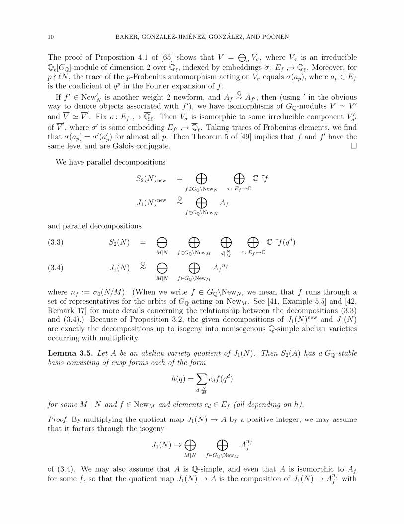
The proof of Proposition 4.1 of [65] shows that V =⊕
σ Vσ, where Vσ is an irreducible
Q`[GQ]-module of dimension 2 over Q`, indexed by embeddings σ : Ef → Q`. Moreover, forp - `N , the trace of the p-Frobenius automorphism acting on Vσ equals σ(ap), where ap ∈ Efis the coefficient of qp in the Fourier expansion of f .
If f ′ ∈ New′N is another weight 2 newform, and AfQ∼ Af ′ , then (using ′ in the obvious
way to denote objects associated with f ′), we have isomorphisms of GQ-modules V ' V ′
and V ' V′. Fix σ : Ef → Q`. Then Vσ is isomorphic to some irreducible component V ′σ′
of V′, where σ′ is some embedding Ef ′ → Q`. Taking traces of Frobenius elements, we find
that σ(ap) = σ′(a′p) for almost all p. Then Theorem 5 of [49] implies that f and f ′ have thesame level and are Galois conjugate.
We have parallel decompositions
S2(N)new =⊕
f∈GQ\NewN
⊕τ : Ef →C
C τf
J1(N)new Q∼⊕
f∈GQ\NewN
Af
and parallel decompositions
S2(N) =⊕M |N
⊕f∈GQ\NewM
⊕d| NM
⊕τ : Ef →C
C τf(qd)(3.3)
J1(N)Q∼
⊕M |N
⊕f∈GQ\NewM
Afnf(3.4)
where nf := σ0(N/M). (When we write f ∈ GQ\NewN , we mean that f runs through aset of representatives for the orbits of GQ acting on NewM . See [41, Example 5.5] and [42,Remark 17] for more details concerning the relationship between the decompositions (3.3)and (3.4).) Because of Proposition 3.2, the given decompositions of J1(N)new and J1(N)are exactly the decompositions up to isogeny into nonisogenous Q-simple abelian varietiesoccurring with multiplicity.
Lemma 3.5. Let A be an abelian variety quotient of J1(N). Then S2(A) has a GQ-stablebasis consisting of cusp forms each of the form
h(q) =∑d| NM
cdf(qd)
for some M | N and f ∈ NewM and elements cd ∈ Ef (all depending on h).
Proof. By multiplying the quotient map J1(N) → A by a positive integer, we may assumethat it factors through the isogeny
J1(N)→⊕M |N
⊕f∈GQ\NewM
Anff
of (3.4). We may also assume that A is Q-simple, and even that A is isomorphic to Affor some f , so that the quotient map J1(N) → A is the composition of J1(N) → A
nff with

MODULAR CURVES OF GENUS AT LEAST 2 11
a homomorphism Anff → A. The latter is given by an nf -tuple c = (cd) of elements of
End(Af ), indexed by the divisors d of N/M . Under
X1(N) → J1(N)→ Anff
c→ A,
the 1-form on AC ' (Af )C corresponding to f pulls back to∑
d| NMcdf(qd) dq/q. Finally,
H0(AC,Ω) has a basis consisting of this 1-form and its conjugates, and the pullbacks ofthese conjugates are sums of the same form.
Corollary 3.6. Let π : X1(N) → X be a nonconstant morphism of curves over Q. ThenS2(X) has a GQ-stable basis T consisting of cusp forms each of the form
h(q) =∑d| NM
cdf(qd)
for some M | N and f ∈ NewM , where cd ∈ Ef depends on f and d.
Proof. Apply Lemma 3.5 to the Albanese homomorphism J1(N)→ JacX.
3.2. Automorphisms of X1(N).
3.2.1. Diamonds. The action on H of a matrix
(a bc d
)∈ Γ0(N) induces an automorphism
of X1(N) over Q depending only on (d mod N). This automorphism is called the diamondoperator 〈d〉. It induces an automorphism of S2(N). Let ε be a Dirichlet character moduloN , that is, a homomorphism (Z/NZ)∗ → C∗. Let S2(N, ε) be the C-vector space h ∈S2(N) : h|〈d〉 = ε(d)h . A form h ∈ S2(N, ε) is called a form of Nebentypus ε. Everynewform f ∈ NewN is a form of some Nebentypus, and is therefore an eigenvector for all thediamond operators. Character theory gives a decomposition
S2(N) =⊕ε
S2(N, ε) ,
where ε runs over all Dirichlet characters modulo N . Define S2(N, ε)new = S2(N, ε) ∩S2(N)new. When we write ε = 1, we mean that ε is the trivial Dirichlet character moduloN , that is,
ε(n) =
1 if (n,N) = 1
0 otherwise.
A form of Nebentypus ε = 1 is a form on Γ0(N).We recall some properties of a newform f =
∑∞n=1 anq
n ∈ S2(N, ε). Let cond ε denotethe smallest integer M | N such that ε is a composition (Z/NZ)∗ → (Z/MZ)∗ → C∗.Throughout this paragraph, p denotes a prime, and denotes complex conjugation. Letvp(n) denote the p-adic valuation on Z. If vp(cond ε) < vp(N), then ε is a composition

12 BAKER, GONZALEZ-JIMENEZ, GONZALEZ, AND POONEN
(Z/NZ)∗ → (Z/(N/p)Z)∗ε′→ C∗ for some ε′. Then
∞∑n=1
ann−s =
∏p
(1− app−s + p ε(p) p−2s)−1,(3.7)
p | N ⇐⇒ ε(p) = 0(3.8)
vp(cond ε) < vp(N) ≥ 2 =⇒ ap = 0(3.9)
vp(cond ε) < vp(N) = 1 =⇒ a2p = ε′(p)(3.10)
1 ≤ vp(cond ε) = vp(N) =⇒ |ap| =√p(3.11)
vp(N) = 1, ε = 1 =⇒ f |Wp = −apf(3.12)
p - N =⇒ ap = ε(p) ap.(3.13)
(The equivalence (3.8) is trivial. Facts (3.7), (3.9), (3.10), (3.11) follow from parts (i), (iii),(iii), (ii) of [49, Theorem 3], respectively. Fact (3.12) follows from (3.10), [6, Theorem 2.1],and lines 6–7 of [6, p. 224]. Fact (3.13) follows from the first case of [6, equation (1.1)] andthe lines preceding it.)
3.2.2. Involutions. For every integer M | N such that (M,N/M) = 1, there is an automor-phism WM of X1(N)C inducing an isomorphism between S2(N, ε)new and S2(N, εMεN/M)new,where εM denotes the character mod M induced by ε. (For more on this action, see [6]).Given a newform f ∈ S2(N, ε), there is a newform εM ⊗ f in S2(N, εMεN/M) whose pth
Fourier coefficient bp is given by
bp =
εM(p)ap if p -M ,
εN/M(p)ap if p |M.
Then
(3.14) f |WM = λM(f)(εM ⊗ f)
for some λM(f) ∈ C with |λM(f)| = 1. Moreover, we have
f |W 2M = εN/M(−M) f , f |(WM ′WM) = εM ′(M)f |WM ′M
whenever (M,M ′) = 1. In the particular case M = N , the automorphism WN is aninvolution defined over the cyclotomic field Q(ζN), called the Weil involution. For allτ ∈ Gal (Q(ζN)/Q), the automorphisms τWN are involutions and are also called Weil in-volutions by some authors. The involution WN maps each S2(Af ) into itself and satisfies
(3.15) 〈d〉WN = WN〈d〉−1 , τdWN = WN 〈d〉 for all d ∈ (Z/NZ)∗ ,
where τd is the element of Gal (Q(ζN)/Q) mapping ζN to ζdN .Let ε be a Dirichlet character modulo N . Define the congruence subgroup
Γ(N, ε) :=
(a bc d
)∈ Γ0(N) | ε(d) = 1
.
Let S2(Γ(N, ε)) denote the space of weight 2 cusp forms on Γ(N, ε). Denote by X(N, ε) themodular curve over Q such that X(N, ε)(C) contains Γ(N, ε)\H as a dense open subset. We

MODULAR CURVES OF GENUS AT LEAST 2 13
can identify H0(X(N, ε)C,Ω) with S2(Γ(N, ε))dqq
. The Dirichlet characters modulo N whose
kernel contains ker(ε) are exactly the powers of ε, so
S2(Γ(N, ε)) =n⊕k=1
S2(N, εk) ,
where n is the order of ε. The diamond operators and the Weil involution induce automor-phisms of X(N, ε)C. If moreover ε = 1, the curve X(N, 1) is X0(N) and the automorphismsWM on X1(N)C induce involutions on X0(N) over Q that are usually called the Atkin-Lehnerinvolutions.
Remark 3.16. Define the modular automorphism group of X1(N) to be the subgroup ofAut(X1(N)Q) generated by the WM ’s and the diamond automorphisms. The quotient ofX1(N) by this subgroup equals the quotient of X0(N) by its group of Atkin-Lehner invo-lutions, and is denoted X∗(N). The genus of X0(N) is N1+o(1) as N → ∞, so by Propo-sition 4.4, the gonality of X0(N) is at least N1+o(1). On the other hand, the degree ofX0(N) → X∗(N) is only 2#prime factors of N = N o(1). Hence the gonality of X∗(N) tends toinfinity. Thus the genus of X∗(N) tends to infinity. In particular, Conjecture 1.1 is trueif one restricts the statement to modular curves X that are quotients of X1(N) by somesubgroup of the modular automorphism group.
3.2.3. Automorphisms of new modular curves. By Proposition 2.11, if X is a new modularcurve of level N and genus g ≥ 2, then the diamond operators and the Weil involutionWN induce automorphisms of XQ, which we continue to denote by 〈d〉 and WN respectively.Throughout the paper, D will denote the abelian subgroup of Aut(XQ) consisting of diamondautomorphisms, and DN := 〈D,WN〉 will denote the subgroup of Aut(XQ) generated by Dand WN . If moreover X is hyperelliptic, and w is its hyperelliptic involution, then the groupgenerated by D and WN .w will be denoted by D′N .
Note that D is a subgroup of Aut(X), and the groups DN , D′N are GQ-stable by (3.15). If
JacXQ∼ Af for some f with nontrivial Nebentypus, then DN is isomorphic to the dihedral
group with 2n elements, D2·n, where n is the order of the Nebentypus of f .
For every nonconstant morphism π : X1(N) → X of curves over Q such that S2(X) ⊆⊕ni=1S2(N, εi) for some Nebentypus ε of order n, there exists a nonconstant morphismπ(ε) : X(N, ε) → X over Q. This is clear when the genus of X is ≤ 1, and follows fromProposition 2.11(i) if the genus of X is > 1. In particular, for a new modular curve X ofgenus > 1, there exists a surjective morphism X0(N) → X if and only if D is the trivialgroup. More generally, we have the following result.
Lemma 3.17. Let X be a new modular curve of level N , and let G be a GQ-stable subgroupof Aut(XQ). Let X ′ = X/G. If the genus of X ′ is at least 2, then the group D′ of diamondsof X ′ is isomorphic to D/(G∩D). In particular, if G = D or DN , then there is a nonconstantmorphism π′ : X0(N)→ X ′ defined over Q.
Proof. By Proposition 2.11, each diamond automorphism of X induces an automorphismof X ′. Hence we obtain a surjective homomorphism ρ : D → D′. Let K = ker(ρ). SinceG∩D ⊆ K, it suffices to show thatK ⊆ G. NowH0(X ′,Ω) pulls back to the spaceH0(X,Ω)G
of G-invariant regular differentials of X, so K acts trivially on the latter. Therefore the resultfollows from Lemma 3.18 below.

14 BAKER, GONZALEZ-JIMENEZ, GONZALEZ, AND POONEN
Lemma 3.18. Let X be a curve over a field of characteristic zero, and let G be a finitesubgroup of Aut(X). Assume that the genus g′ of X ′ := X/G is at least 2. Let
G := φ ∈ Aut(X) : φ∗ω = ω for all ω ∈ H0(X,Ω)G .
Then G = G.
Proof. It is clear that G ⊆ G. Now suppose φ ∈ G, and let H := 〈G, φ〉. Also, setX ′′ := X/H, and let g′′ be the genus of X ′′. Then there is a natural dominant morphismπ : X ′ → X ′′. Moreover,
g′′ = dimH0(X,Ω)H = dimH0(X,Ω)〈G,φ〉 = dimH0(X,Ω)G = g′.
Since g′ ≥ 2 by hypothesis, the Hurwitz formula implies deg(π) = 1. Therefore φ ∈ G, sothat G ⊆ G as required.
3.3. Supersingular points. We will use a lemma about curves with good reduction.
Lemma 3.19. Let R be a discrete valuation ring with fraction field K. Suppose f : X → Y isa finite morphism of smooth, projective, geometrically integral curves over K, and X extendsto a smooth projective model X over R (in this case we say that X has good reduction). IfY has genus ≥ 1, then Y extends to a smooth projective model Y over R, and f extends toa finite morphism X → Y over R.
Proof. This result is Corollary 4.10 in [50]. See the discussion there also for references toearlier weaker versions.
The next two lemmas are well-known, but we could not find explicit references, so wesupply proofs.
Lemma 3.20. Let p be a prime. Let Γ ⊆ SL2(Z) denote a congruence subgroup of level Nnot divisible by p. Let XΓ be the corresponding integral smooth projective curve over Q, andlet ψ be the degree of the natural map XΓ → X(1). Then XΓ has good reduction at any placeabove p, and the number of Fp-points on the reduction mapping to supersingular points onX(1) is at least (p− 1)ψ/12.
Proof. By [39], the curve X(N) admits a smooth model over Z[1/N ], and has a rationalpoint (the cusp ∞). Since p - N and X(N) dominates XΓ, Lemma 3.19 implies that XΓ hasgood reduction at p, at least if XΓ has genus ≥ 1. If XΓ has genus 0, then the rational pointon X(N) gives a rational point on XΓ, so XΓ ' P1, so XΓ has good reduction at p in anycase. Replacing Γ by the group generated by Γ and − id does not change XΓ, so withoutloss of generality, we may assume that − id ∈ Γ. Then ψ = (SL2(Z) : Γ).
If E is an elliptic curve, then Γ naturally acts on the finite set of ordered symplectic basesof E[N ]. The curve YΓ := XΓ−cusps classifies isomorphism classes of pairs (E,L), whereE is an elliptic curve and L is a Γ-orbit of symplectic bases of E[N ].
Fix E. Since SL2(Z) acts transitively on the symplectic bases of E[N ], the number ofΓ-orbits of symplectic bases is (SL2(Z) : Γ) = ψ. Two such orbits L and L′ correspond tothe same point of XΓ if and only if L′ = αL for some α ∈ Aut(E). Then ψ is the sum of thesizes of the orbits of Aut(E) acting on the Γ-orbits, so
ψ =∑
(E,L)∈XΓ
#Aut(E)
#Aut(E,L),
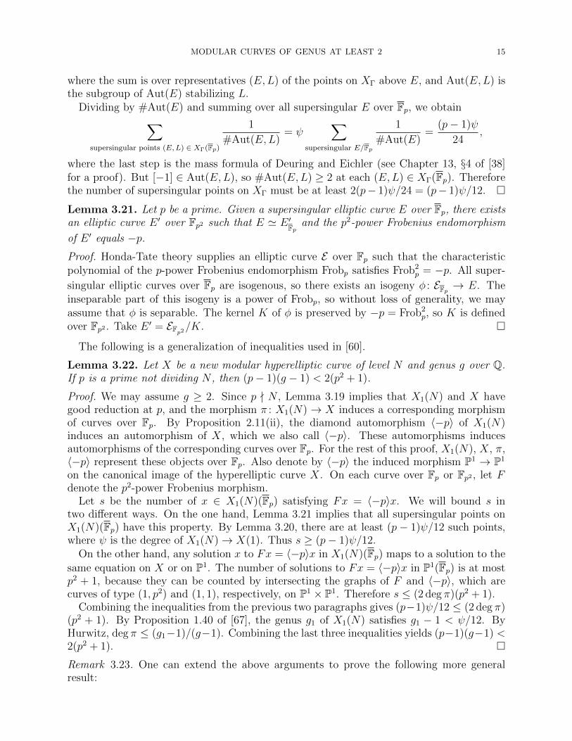
MODULAR CURVES OF GENUS AT LEAST 2 15
where the sum is over representatives (E,L) of the points on XΓ above E, and Aut(E,L) isthe subgroup of Aut(E) stabilizing L.
Dividing by #Aut(E) and summing over all supersingular E over Fp, we obtain∑supersingular points (E,L) ∈ XΓ(Fp)
1
#Aut(E,L)= ψ
∑supersingular E/Fp
1
#Aut(E)=
(p− 1)ψ
24,
where the last step is the mass formula of Deuring and Eichler (see Chapter 13, §4 of [38]for a proof). But [−1] ∈ Aut(E,L), so #Aut(E,L) ≥ 2 at each (E,L) ∈ XΓ(Fp). Thereforethe number of supersingular points on XΓ must be at least 2(p− 1)ψ/24 = (p− 1)ψ/12.
Lemma 3.21. Let p be a prime. Given a supersingular elliptic curve E over Fp, there existsan elliptic curve E ′ over Fp2 such that E ' E ′Fp and the p2-power Frobenius endomorphism
of E ′ equals −p.
Proof. Honda-Tate theory supplies an elliptic curve E over Fp such that the characteristicpolynomial of the p-power Frobenius endomorphism Frobp satisfies Frob2
p = −p. All super-
singular elliptic curves over Fp are isogenous, so there exists an isogeny φ : EFp → E. Theinseparable part of this isogeny is a power of Frobp, so without loss of generality, we mayassume that φ is separable. The kernel K of φ is preserved by −p = Frob2
p, so K is definedover Fp2 . Take E ′ = EFp2/K.
The following is a generalization of inequalities used in [60].
Lemma 3.22. Let X be a new modular hyperelliptic curve of level N and genus g over Q.If p is a prime not dividing N , then (p− 1)(g − 1) < 2(p2 + 1).
Proof. We may assume g ≥ 2. Since p - N , Lemma 3.19 implies that X1(N) and X havegood reduction at p, and the morphism π : X1(N)→ X induces a corresponding morphismof curves over Fp. By Proposition 2.11(ii), the diamond automorphism 〈−p〉 of X1(N)induces an automorphism of X, which we also call 〈−p〉. These automorphisms inducesautomorphisms of the corresponding curves over Fp. For the rest of this proof, X1(N), X, π,〈−p〉 represent these objects over Fp. Also denote by 〈−p〉 the induced morphism P1 → P1
on the canonical image of the hyperelliptic curve X. On each curve over Fp or Fp2 , let Fdenote the p2-power Frobenius morphism.
Let s be the number of x ∈ X1(N)(Fp) satisfying Fx = 〈−p〉x. We will bound s intwo different ways. On the one hand, Lemma 3.21 implies that all supersingular points onX1(N)(Fp) have this property. By Lemma 3.20, there are at least (p− 1)ψ/12 such points,where ψ is the degree of X1(N)→ X(1). Thus s ≥ (p− 1)ψ/12.
On the other hand, any solution x to Fx = 〈−p〉x in X1(N)(Fp) maps to a solution to the
same equation on X or on P1. The number of solutions to Fx = 〈−p〉x in P1(Fp) is at mostp2 + 1, because they can be counted by intersecting the graphs of F and 〈−p〉, which arecurves of type (1, p2) and (1, 1), respectively, on P1 × P1. Therefore s ≤ (2 deg π)(p2 + 1).
Combining the inequalities from the previous two paragraphs gives (p−1)ψ/12 ≤ (2 deg π)(p2 + 1). By Proposition 1.40 of [67], the genus g1 of X1(N) satisfies g1 − 1 < ψ/12. ByHurwitz, deg π ≤ (g1−1)/(g−1). Combining the last three inequalities yields (p−1)(g−1) <2(p2 + 1).
Remark 3.23. One can extend the above arguments to prove the following more generalresult:

16 BAKER, GONZALEZ-JIMENEZ, GONZALEZ, AND POONEN
Let X be a new modular curve of genus g and level N , with p - N . SupposeX admits a degree d map (defined over Q) to a curve X ′/Q of genus g′.Finally, suppose that the diamond automorphisms on X1(N) are compatiblewith automorphisms of X ′. (This is automatic if g′ ≥ 2, or if g ≥ 2, g′ = 0,and d = 2.) Then (g − 1)(p− 1) ≤ d(p2 + 1 + 2pg′).
We omit the proof, since we will not use this result.
Corollary 3.24. Let X be a new modular hyperelliptic curve of level N and genus g overQ. If g > 10, then 6|N . If g > 13, then 30|N .
Proof. Take p = 2, 3, and 5 in Lemma 3.22.
In the case where X is a curve dominated by X0(N), 〈−p〉 is the identity, so in the proofof Lemma 3.22 we may replace the bound (2 deg π)(p2 + 1) by (deg π)#X(Fp2) to obtain thefollowing:
Lemma 3.25. Suppose that X is a curve of genus g ≥ 2 over Q, and π : X0(N) → X is adominant morphism over Q. Suppose that p is a prime not dividing N . Then X has goodreduction at p, and (p − 1)(g − 1) < #X(Fp2). In particular, if GQ denotes the Q-gonality
of X, then g < GQp2+1p−1
+ 1.
3.4. Previous work on curves dominated by modular curves. Except for the deter-mination of all new modular genus-2 curves with Q-simple jacobian in [27], all work we knowof on modular curves of genus ≥ 2 has focused on X0(N), X1(N), or quotients of these bya subgroup of the group of Atkin-Lehner involutions or diamonds, respectively. Here wesummarize some of this work.
The 19 values of N for which X0(N) is hyperelliptic (of genus ≥ 2) were determinedin [60], and all of their equations were given in [26]. The corresponding determination of thethree values of N for which X1(N) is hyperelliptic was carried out in [55], and equations forthese (and a few other X1(N)) were given in [63]. In [40] it is proved that a curve strictlybetween X0(N) and X1(N) (that is, a quotient of X1(N) by a nontrivial proper subgroupof the diamond group) is never hyperelliptic. A series of works [46], [31], [30] led up to thedetermination of all 64 values of N for which the quotient of X0(N) by its Atkin-Lehnergroup, X∗(N), is hyperelliptic, and this was generalized in [23] to quotients of X0(N) byan arbitrary subgroup of the Atkin-Lehner group. Similar results determining all trigonalcurves of the form X0(N), X0(N)/Wd for a single Atkin-Lehner involution Wd, and X∗(N),can be found in [32], [33], and [34], respectively. Some of these curves are not new, and hencedo not appear in our tables.
The method of constructing equations for modular curves one at a time in terms of abasis of cusp forms has been used by many authors: in addition to the papers alreadymentioned, we have [58], [70], [24], for instance. In particular, [70] gives methods for boththe hyperelliptic and nonhyperelliptic cases, using Petri’s Theorem in the latter, as we do.F. Klein [45] gave an explicit model for X(p) for every prime p in 1879. See [75] for a modernconstruction of X(N) for every N . An analogous result for X1(p) can be found in [7].
4. Finiteness theorems
Our goal in this section is to prove the finiteness statements in Theorems 1.3, 1.5, and 1.8.Algorithmic and practical issues will be dealt with only in later sections, because we assume

MODULAR CURVES OF GENUS AT LEAST 2 17
that some readers will be interested only in the finiteness. In particular, the computability ofthe sets in question will be proved in Section 5, and practical algorithms in the hyperellipticcase will be given in Section 6.
4.1. New modular curves of fixed genus.
Proof of finiteness in Theorem 1.3. Fix g ≥ 2. Let X be a new modular curve of level N andgenus g, given by the nonconstant morphism π : X1(N) → X. Since the Q-simple factorsAf of J1(N)new are pairwise nonisogenous, any abelian subquotient of J1(N)new is isogenousto a product of some subset of these Af . Applying this to J = JacX and then comparing1-forms shows that there exists a GQ-stable subset T ⊆ NewN that is a basis for S2(X).
¿From now on, let f = q+a2q2+a3q
3+· · · denote an element of T . The map π is unramifiedat∞, since there exists ω ∈ H0(XC,Ω) such that π∗ω = f dq/q, which is nonvanishing at∞.In other words, the analytic uniformizer q at∞ on X1(N) serves also as analytic uniformizerat π(∞) on X.
The field Ef generated by the coefficients of f satisfies [Ef : Q] = dimAf ≤ dim J = g.Let B be the integer of Proposition 2.1. Each an for 1 ≤ n ≤ B is an algebraic integer ofdegree at most g, bounded in every archimedean absolute value by σ0(n)
√n, so there are
only finitely many possibilities for an. Thus there are only finitely many possibilities for f mod qB | f ∈ T , given g. By Proposition 2.1 and Remark 2.6, each such possibilityarises for at most one curve over Q.
Remark 4.1. For this proof, any bound on the absolute values of |an| in terms of n wouldhave sufficed. But when we do computations, it will be useful to have the strong boundσ0(n)
√n.
4.2. Non-new modular curves of fixed genus. Our goal in this section is to prove thefiniteness assertion of Theorem 1.5.
Proof of finiteness in Theorem 1.5(i). Let X/Q be a modular curve of genus g ≥ 2 and levelN , so that there exists a map π : X1(N) → X over Q. Let B = B(g) be the integer ofProposition 2.1.
We will follow the basic strategy of the proof of Theorem 1.3, but two complications arise:the map π need not be unramified at ∞, and the cusp forms whose Fourier coefficients weneed to bound need not be newforms. The sparseness assumption will allow us to get aroundboth of these difficulties.
Let T be as in Corollary 3.6. Choose j ∈ T with ordq(j) minimal. Then j dq/q correspondsto a regular differential on XC not vanishing at π(∞). Since q is an analytic parameter at∞ on X1(N), the ramification index e of π at ∞ equals ordq(j). In particular, e|N . ByRemark 2.7, the curve X is determined by the set h mod qeB |h ∈ T .
Fix h =∑∞
n=1 anqn ∈ T . Since ordq(h) ≥ e, Corollary 3.6 implies that there exist an
integer M |N , a newform f ∈ NewM , and cd ∈ C such that
h =∑
d| NM,d≥e
cdf(qd).
Since N ∈ SparseB, we have d > eB for all d | N such that d > e. If ce = 0, thenh mod qeB = 0; otherwise we may scale to assume that ce = 1. In this case, the sparseness

18 BAKER, GONZALEZ-JIMENEZ, GONZALEZ, AND POONEN
of N implies that an(h(q)) = an(f(qe)) for 1 ≤ n < eB. In other words, for 1 ≤ n < eB wehave
an(h) =
an/e(f) if e | n,
0 if e - n.
Since f is a newform, each an(h) with n ≤ eB and e|n is an algebraic integer satisfying
|an(h)| ≤ σ0(n/e)√n/e for all archimedean absolute values. As before, it then follows that
there are only finitely many possibilities for h mod qeB |h ∈ T , and therefore for X.
Proof of finiteness in Theorem 1.5(ii). Let X/Q be a modular curve of genus g ≥ 2 and levelN ∈ Smoothm, with m > 0. Then JacX is isogenous to a subvariety of J1(N), so in particularJacX has good reduction outside the finite set Σ, where Σ is the set of primes p such thatp ≤ m. By combining the Shafarevich conjecture (proved by Faltings [22, Theorem 6])with a well-known finiteness result for polarizations (see [56, Theorem 18.1]), it follows thatfor any number field K, any positive integer d, and any finite set S of places of K, thereare only finitely many K-isomorphism classes of principally polarized abelian varieties ofdimension d over K with good reduction outside S. In particular, there are only finitelymany possible Q-isomorphism classes for JacX as a principally polarized abelian variety. Bythe Torelli theorem [57, Corollary 12.2], it follows that there are only finitely many possibleQ-isomorphism classes for X.
As mentioned in the introduction, part (iii) of Theorem 1.5 (concerning prime power levels)follows from (i) and (ii).
To close this section, we remark that for modular curves of prime power level (as opposedto general non-new modular curves), one has good control over the ramification at the cuspinfinity. More precisely:
Proposition 4.2. Suppose that N = pr is a prime power. Suppose that X is modular oflevel N but not modular of level M for any M < N . Then the map π : X1(N) → X isunramified at ∞.
Proof. Corollary 3.6 says that S2(X) has a basis in which each element h has the form∑d| NMcdf(qd) for some M |N and f ∈ NewM . If π is ramified at ∞, then c1 = 0 in each
such h. Then∑
d| NM, d>1 cdf(qd/p) ∈ S2(pr−1), according to the decomposition (3.3). Thus
π∗H0(XC,Ω) ⊆ B∗pH0(X1(pr−1)C,Ω), where Bp : X1(pr)→ X1(pr−1) denotes the degeneracy
map induced by q 7→ qp. By Proposition 2.11(i), π factors through X1(pr−1), contradictingthe minimality of N .
4.3. New modular curves of fixed gonality. In [2, p. 1006], one finds the following lowerbound on the gonality of X1(N).
Theorem 4.3. Let g′ and G′ be the genus and gonality, respectively, of X1(N). ThenG′ ≥ 21
200(g′ − 1).
The linearity of the bound in the genus ofX1(N) is what enables us to deduce the following.
Proposition 4.4. If X is a C-modular curve of genus g ≥ 2 and gonality G, then g ≤20021G+ 1.

MODULAR CURVES OF GENUS AT LEAST 2 19
Proof. Let d be the degree of the given morphism π : X1(N)C → X. Let g′ and G′ be thegenus and gonality of X1(N), so that G′ ≥ 21
200(g′ − 1) by Theorem 4.3. Any morphism
X → P1C can be composed with π to obtain a morphism X1(N)C → P1
C, so G′ ≤ dG. TheHurwitz formula implies g′ − 1 ≥ d(g − 1). Now combine these three inequalities.
Proposition 4.4 and Theorem 1.3 together imply the finiteness in Theorem 1.8.
Remark 4.5. Abramovich’s result used the lower bound 0.21 for the positive eigenvalues ofthe Laplacian on Γ\H for congruence subgroups Γ. In Appendix 2 to [44], Kim and Sarnakrecently improved this to 975/4096 > 0.238. This means that 200/21 can be improved to2/0.238 < 17/2. In particular, taking G = 2, we find that a C-modular hyperelliptic curvehas genus at most 17.
5. Computability
5.1. The meaning of computable. “Computable” will mean computable by a Turingmachine. (See [37] for a definition of Turing machine.) To give a precise sense to eachstatement in our introduction, we must specify what the input and output of the Turingmachine are to be. In particular, we will need to choose how to represent various objects,such as curves over number fields. In many cases, there exist algorithms for convertingbetween various possible representations, so then the particular representation chosen is notimportant. A number field k can be represented by f ∈ Z[x] such that k ' Q[x]/(f(x)).The representation is not unique, but we do not care, since a Turing machine can decide,given f1, f2 ∈ Z[x], whether f1 and f2 define isomorphic number fields (and if so, find anisomorphism) [48, §2.9]. An element α ∈ k can then be represented by g ∈ Q[x] (of degreeat most deg f − 1) whose image in Q[x]/(f(x)) corresponds to α. Turing machines can alsohandle arithmetic over Q, thought of as a subfield of C, by representing each α ∈ Q by itsminimal polynomial over Q, together with decimal approximations to its real and imaginaryparts to distinguish α from its conjugates. If k0 = Q or k0 = Q, then a field finitely generatedover k0 can be represented as the fraction field of a domain k0[t1, . . . , tn]/(f1, . . . , fm), oralternatively as a finite extension of the rational function field k0(t1, . . . , tn) (in the sameway that we handled finite extensions of Q).
A curve X over a field k finitely generated over Q or Q can be represented by f ∈ k[x, y]such that the (possibly singular) affine curve f(x, y) = 0 is k-birational to X. Meromorphicdifferentials on X represented by f ∈ k[x, y] can be expressed as g(x, y) dx or g(x, y) dy,where g = g1/g2 with g1, g2 ∈ k[x, y] and g2 not divisible by f . A finite set of k-isomorphismclasses of curves over k can be represented by a finite list of curves over k in which each classis represented exactly once.
A closed subvariety of Pn over a field k finitely generated over Q or Q can be representedby a finite set of generators of its homogeneous ideal. A constructible subset of Pn (inthe Zariski topology) can be represented as a Boolean combination of closed subvarieties.Morphisms or rational maps between quasiprojective varieties can be defined locally byrational functions on a finite number of affine open subsets. Elimination of quantifiers overalgebraically closed fields is effective, and it follows that the image of a constructible subset ofa quasiprojective variety under a morphism can be computed. (The elimination of quantifiersis usually attributed to Tarski; for a proof, see Section 3.2 of [53], especially Theorem 3.2.2and Corollary 3.2.8(ii).) Irreducible components of a variety can also be computed: thisfollows from the primary decomposition algorithm in [35].

20 BAKER, GONZALEZ-JIMENEZ, GONZALEZ, AND POONEN
When in one of our theorems we claim that some set is computable, what we really meanis that there exists a Turing machine that takes as input the various parameters on whichthe set depends (such as a ground field, a curve, and/or an integer g), and, after a finite butunspecified amount of computation, terminates and outputs the set in question.
5.2. Computability lemmas for curves.
Lemma 5.1. A Turing machine can solve the following problems: Given a field k finitelygenerated over Q or Q, and given curves X and Y over k,
(1) Compute the genus g of (the smooth projective model of) X.(2) If g ≥ 2, decide whether or not X is hyperelliptic.(3) If either of the following holds:
(i) g(X) ≥ 2(ii) g(X) = 0 and k is a number field or Q,
decide whether X and Y are k-birational.
Proof.(1) See [1].(2) See [74].(3) By (1) we may assume that X and Y have the same genus g, and that g is known. If
g ≥ 2, use [36]. From now on, suppose that g = 0. If k = Q, then X and Y are automaticallybirational. So from now on, suppose that k is a number field. By [73], we can find planeconics birational to X and Y , respectively. Diagonalize the corresponding quadratic forms toput each curve in the form x2− ay2− bz2 = 0 for some a, b ∈ k∗. By the Hasse principle, thecurves are isomorphic over k if and only if the order-2 Hilbert symbols (a, b)v match at everyplace v. In fact, one need only check the places above 2 and∞ and the places occuring in thefactorizations of the a and b for each curve. Each Hilbert symbol is computable: see [18] orII.7.1.5 and II.7.5 in [29]. (Alternatively, the question of whether the conic x2−ay2−bz2 = 0has a kv-point can be answered by taking its restriction of scalars down to Q and using ageneral algorithm for deciding whether a variety over Q has a Qp-point: see [72] or [59] forthe archimedean and nonarchimedean cases, respectively.)
Remark 5.2. Most of these algorithms have been fully implemented. For instance, Magma [8]can compute the genus of a plane curve, and PARI-GP at http://www.parigp-home.de/
has a function nfhilbert for computing Hilbert symbols.
Remark 5.3. Lemma 5.1(3) holds in the genus 1 case if and only if there exists an algorithmto decide, given a genus 1 curve Z over k, whether Z(k) = ∅. Such an algorithm existstrivially if k = Q. If k is a number field, the existence of such an algorithm is implied by theconjecture that the Shafarevich-Tate group X(E) is finite for all elliptic curves E over k.
Lemma 5.4. Let X be a curve over a number field k, and let ` ≥ 1 be an integer. LetA = JacX, and let M = A[`] be the Galois module of `-torsion points. Then we can computea description of M of the following type: a finite set equipped with an addition table and anaction of Gal (L/k) for some explicit finite Galois extension L of k over which all points ofM are defined.
Proof. Compute the genus g of X. We represent points of A(Q) (nonuniquely) by divisors onXQ whose support avoids any singularities of the given model. A solution of the “Riemann-Roch problem” decides whether a given divisor is principal: see the references cited in [61].

MODULAR CURVES OF GENUS AT LEAST 2 21
Hence we can decide when two given divisors represent the same element of A(Q). Nowenumerate the countably many divisors on XQ avoiding the singularities, and continue until
finding a set S of `2g such divisors D such that `D is principal, and such that they representdistinct elements of A(Q). For each pair in S, we can determine which divisor in S is linearlyequivalent to their sum. Finally, we can compute a finite Galois extension L of k containingthe coordinates of all points appearing in the divisors in S, and for each σ ∈ Gal (L/k) andD ∈ S, we can determine which divisor in S is linearly equivalent to σD.
Lemma 5.5. Given a Galois extension of number fields L/k, the set of ramified primes ink and the sequence of ramification groups for each ramified prime are computable.
Proof. By Sections 2.2.4 and 2.3.5 respectively of [14], we can compute the relative discrimi-nant ideal and factor it to obtain the ramified primes. For each ramified prime p of k, we use[14, Algorithm 2.5.4] to extend it to an ideal of L, factor it to obtain a prime P of L abovep, and use [14, §2.2.3] find an element α ∈ P of P-adic valuation 1. For each σ ∈ Gal (L/k),we compute the valuation of σα− α: this determines the ramification groups.
Proposition 5.6. The conductor of the jacobian of a curve X over a number field k iscomputable.
Proof. Let ` ∈ Z be a prime, and let A = JacX. Compute A[`] and L as in Lemma 5.4.Use Lemma 5.5 to compute the ramification groups of Gal (L/k) at each ramified prime ofk. Their action on A[`] gives us the exponent of p in cond(A) for each p not dividing `.Repeating the above with a different ` lets us compute the remaining exponents.
5.3. The de Franchis-Severi Theorem. The following result, which we have alreadymentioned, is known as the de Franchis-Severi Theorem; we show in addition that the finiteset it promises is computable. We thank Matthias Aschenbrenner, Brian Conrad, TomGraber, Tom Scanlon, and Jason Starr for discussions related to the proof.
Theorem 5.7 (de Franchis-Severi, computable version). Let k be a number field or Q. LetX be a curve over k. Then the set of pairs (Y, π) where Y is a curve over k of genus at least2 and π : X → Y is a morphism, up to k-isomorphism, is finite and computable.
Remark 5.8. We consider (Y, π) and (Y ′, π′) to be isomorphic if and only if there is anisomorphism Y → Y ′ whose composition with π gives π′.
Proof. For the finiteness, see pp. 223–224 of [47]. We assume first that k = Q. The genus gof each Y is bounded by the genus gX of X, so it suffices to show that for each fixed g ≥ 2,we can compute the set Cg of isomorphism classes of pairs (Y, π) where Y has genus g.
View X as a subvariety of Pn using the tricanonical embedding. Compute equationsdefining X in Pn. If (Y, π) ∈ Cg and Y ⊆ Pm is the tricanonical embedding of Y , then3KX − π∗(3KY ) is linearly equivalent to an effective divisor, so the theory of linear systemsimplies that there is a linear subspace L ⊆ Pn of dimension n−m− 1 such that π and thelinear projection πL : Pn 99K Pm coincide on X − L. Riemann-Roch gives n = 5gX − 6 andm = 5g−6. Let G be the Grassmannian variety whose points correspond to linear subspacesL ⊆ Pn of dimension n−m− 1. Then (Y, π) 7→ L defines an injection ι : Cg → G(Q).
Conversely, if we start with a linear subspace L, corresponding to a point s ∈ G, let Ys bethe Zariski closure of πL(X−L) in Pm, and let πs : X → Ys denote the morphism induced byπL. The map s 7→ (Ys, πs) restricted to ι(Cg) is an inverse of ι, but in general (Ys, πs) neednot be in Cg. Moreover, the Ys need not form the fibers of a smooth (or even flat) family.

22 BAKER, GONZALEZ-JIMENEZ, GONZALEZ, AND POONEN
Claim 1: Each closed subvariety H ⊆ G can be (computably) partitioned into a finitenumber of irreducible locally closed subsets Hi such that for each i, either
(1) For all s ∈ Hi, the curve Ys is not smooth over the residue field of s, or(2) There is a smooth family Y → Hi of curves, and an Hi-morphism X ×k Hi → Y
whose fiber above s ∈ Hi is πs : X → Ys.
Proof: We use induction on dimH. Because irreducible components can be computed, wemay reduce to the case where H is irreducible.
We next use the principle that “whatever happens at the generic point also happens oversome computable dense Zariski open subset.” Let η be the generic point of H, and let L bethe corresponding linear subspace defined over the function field κ of H. Choose a dense openaffine subset SpecA of H, and write elements of κ as ratios of elements of A. Working over κ,we compute the intersection of L with X, the image of X−L under the projection Pn 99K Pm,its closure Yη, and the morphism πη : X → Yη. Using partial derivatives, we compute alsowhether or not Yη is smooth over κ. Compute the localization A′ of A obtained by adjoiningto A the inverses of the numerators and denominators of the finitely many elements of κthat appear during these computations. Then the formulas computed over κ make senseover SpecA′, so that all the constructions can be performed over SpecA′. Moreover, for eachs ∈ SpecA′, the curve Ys is smooth over the residue field of s if and only if Yη is smooth overκ.
Let H1 = SpecA′ ⊆ H. The complement H−H1 is a closed subvariety of lower dimensionthan H, so using the inductive hypothesis, we can partition H −H1 into H2, . . . , Hn withthe desired properties. This completes the proof of Claim 1.
Apply Claim 1 to G, and discard the Hi in which the Ys are not smooth. For eachremaining Hi, the genus of Ys is constant for s ∈ Hi, so we compute the genus of the genericfiber Yη and discard Hi if this genus is not g.
Claim 2: For each remaining Hi, let Ji be the set of s ∈ Hi for which the linear subspaceL ⊆ Pn corresponding to s equals the linear subspace L′ ⊆ Pn defined as the common zerosof the sections in the image of H0(Ys, ω
⊗3) → H0(X,ω⊗3). Then Ji is constructible andcomputable.
Proof: The strategy of proof is the same as that of Claim 1. The equality of L andL′ can be tested at the generic point η of Hi, and the outcome will be the same on somecomputable dense Zariski open subset of Hi. We finish the proof of Claim 2 by an inductionon the dimension.
Let J be the (computable) union of the Ji. By definition, J = ι(Cg). Since Cg is finite, Jis finite. Therefore Cg can be computed by computing (Ys, πs) for s ∈ J . This completes the
proof of Theorem 5.7 in the case where k = Q.
Finally, suppose that k is a number field. Compute the finite subset J for k = Q as above.Since ι is Gk-equivariant, it suffices to compute the Gk-invariant elements of J . For eachL ∈ J ⊆ G, we compute the Plucker coordinates for L relative to a k-basis of H0(X,ω⊗3),and discard those for which the Plucker embedding does not map L to a k-point of projectivespace. The (Ys, πs) corresponding to the remaining elements of J are the ones over k, eachappearing once.
Remark 5.9. Suppose that k is a number field. Then the finiteness of the set of Y (withoutthe morphism) in Theorem 5.7 holds even if we include curves Y of genus ≤ 1! It is also

MODULAR CURVES OF GENUS AT LEAST 2 23
possible to compute a finite set of curves over k representing all the k-isomorphism classesof such Y , but with some classes represented more than once. Eliminating the redundancyin genus 1 would require an algorithm as in Remark 5.3.
5.4. Computability of modular curves. Here we use the results of the previous sectionto prove that the finite sets in Theorems 1.3, 1.8, and 1.10 are computable.
Proposition 5.10. Fix N ≥ 1 and a number field k. The set of k-modular curves of leveldividing N up to k-isomorphism is finite and computable.
Proof. By Theorem 5.7, it suffices to compute X1(N). First compute the genus g of X1(N)(a formula can be found in Example 9.1.6 on page 77 of [20], for example). Using modularsymbols we can compute a basis of S2(N), with each q-expansion computed up to an error ofO(qB(g)+1). (This follows from [52], and an explicit method was described first in [54, §4.3]:see also the earlier paper [16] and the later thesis [71] for some related work.) Multiplyingeach basis element by dq/q results in expansions for a basis of differentials, and then Sec-tion 2.1 explains how to recover either an equation y2 = f(x) if X1(N) is hyperelliptic, orequations defining the image of the canonical embedding if X1(N) is not hyperelliptic. Inthe latter case, we can try various linear projections and use elimination theory until we findone that yields a plane curve birational to X1(N): we can detect whether a linear projectionmapped the canonical model birationally by checking the genus of the image. Since we canenumerate all linear projections, we will eventually find one that will work. (In practice,almost any projection will work.)
Question 5.11. The de Franchis-Severi Theorem lets us prove the finiteness of modularcurves of fixed level whether or not they are new. Can the proof of the de Franchis-SeveriTheorem somehow be combined with our proof of Theorem 1.3 to prove Conjecture 1.1 ingeneral?
Proof of computability in Theorems 1.3, 1.8, and 1.10. The proof of finiteness in Theorem 1.3produces a finite list of candidate curves X. For each X, we compute N := cond(JacX)1/g,which will be the level of X if X is a new modular curve of genus g and level N . (If N isnot an integer, discard X immediately.) By Proposition 5.10, we can list all modular curvesof level N . Lemma 5.1(3) determines if X is birational to a curve in this list; discard X ifnot. If X is in this list, then it is modular of genus g and level N , and it must be new, sinceotherwise cond(JacX) would be less than N g. Thus we can obtain a list of all new modularcurves of genus g. Finally, we can use Lemma 5.1(3) to eliminate redundancy.
Computability in Theorem 1.8 now follows from computability in Theorem 1.3 and Propo-sition 4.4. Computability in Theorem 1.10 follows from computability in Theorem 1.8 andProposition 7.4.
Remark 5.12. We now explain the difficulty in proving computability of the sets in Theo-rem 1.5. In the proof of finiteness in part (i) (with S = SparseB(g)), we obtained a finite listof candidates X. The problem is that we do not know how to bound the level of a givennon-new modular curve; in fact, we do not even know how to test if a curve is modular. Thelevels of the modular forms corresponding to the regular differentials on X can be boundedby the conductor of the jacobian of X, but this is not enough, since the level of X can behigher than the levels of these forms: see Section 8.2.
Our proof of Theorem 1.5(ii) is ineffective, because there is no known effective proof ofthe Shafarevich conjecture.

24 BAKER, GONZALEZ-JIMENEZ, GONZALEZ, AND POONEN
6. New modular hyperelliptic curves
By Theorem 1.8, the set of the new modular hyperelliptic curves over Q is finite. ByRemark 4.5, the genus of such a curve is ≤ 17. The goal of this section is to improvethis by proving Theorem 1.9 and other restrictions on these curves. The main results aresummarized in Table 1 and proved in Section 6.3. The computational results are given intables in the appendix, and summarized in Section 6.5.
6.1. Criterion to determine new modular hyperelliptic curves. In this subsectionwe will characterize effectively the class of new modular hyperelliptic curves. From now on,for a hyperelliptic curve X we denote by WP(X) the set of Weierstrass points of X.
Lemma 6.1. Assume that there exists a nonconstant morphism π : X1(N)C → X of curvesover C such that X is hyperelliptic of genus g and π∗H0(X,Ω) = H0(AC,Ω), for some
abelian variety A over Q which is a quotient of J1(N)new. We denote by f (j) =∑
n≥1 a(j)n qn,
1 ≤ j ≤ g, a basis for S2(A) consisting of elements of NewN , and we set P = π(∞). Then:
(1) There exists a unique basis h1, . . . , hg of S2(A) such that for all 1 ≤ j ≤ g:hj ≡ qj (mod qg+1) if P 6∈WP(X) ,
hj ≡ q2j−1 +∑g−1
i=j Cj,2i q2i (mod q2g) if P ∈WP(X).
(2) Moreover,
(i) If P 6∈WP(X), then det(a(j)i )1≤i,j≤g 6= 0 .
(ii) If P ∈WP(X), then det(a(j)2i−1)1≤i,j≤g 6= 0 .
Proof. Applying Lemma 2.5 and the fact that π is unramified at the cusp ∞, we obtain theexistence of a basis h′1, . . . , h
′g of S2(A) which satisfies:
h′j ≡ q2j−1 (mod q2j) if P ∈WP(X)
h′j ≡ qj (mod qj+1) if P 6∈WP(X)
for all 1 ≤ j ≤ g. Therefore, (1) is obtained by Gaussian elimination. To obtain (2), itsuffices to observe that the matrices in (i) and (ii) are the change of basis matrices fromf (j) to the basis hj.
Remark 6.2. Later, in Proposition 6.7, we prove that if P ∈ WP(X) then a(j)2n = 0 for all
n ≥ 1 and j ≤ g. In particular, 4 | N and the basis hj satisfies
hj ≡ q2j−1 (mod q2g) .
Remark 6.3. If moreover X comes from a curve over Q having jacobian isogenous to Af withf = q +
∑n≥2 anq
n ∈ NewN , then part (2) of the lemma implies that 1, a2, . . . , ag (resp.1, a3, . . . , a2g−1) is a Q-basis of Ef if P /∈WP(X) (resp. P ∈WP(X)).
Remark 6.4. If A is a quotient of J1(N) (over Q), and the C-vector space S2(A) has a basish1, . . . , hg as in part (1) of the previous lemma, then each hi has Fourier coefficients in Q,since S2(A) has a basis contained in Q[[q]].
The following proposition provides us with an effective criterion to determine when a Q-factor of J1(N)new is Q-isogenous to the jacobian of a modular hyperelliptic curve of levelN . Let 〈v1, . . . , vn〉 denote the span of elements v1, . . . , vn of a vector space.

MODULAR CURVES OF GENUS AT LEAST 2 25
Proposition 6.5. Let A be a quotient of J1(N)new of dimension g > 1. The followingconditions are equivalent:
(1) There exists a modular hyperelliptic curve X of level N over Q such that JacXQ∼ A.
(2) There exists a hyperelliptic curve X ′ over C and a nonconstant morphism π′ : X1(N)C →X ′ such that π′∗H0(X ′,Ω) = H0(AC,Ω).
(3) There exists a basis h1, . . . hg of S2(A) as in part (1) of Lemma 6.1 such that forevery pair g1, g2 ∈ S2(A) satisfying 〈g1, g2〉 = 〈hg−1, hg〉 and g2 ∈ 〈hg〉, there existsF (U) ∈ C[U ] of degree 2g + 1 or 2g + 2 without double roots such that the functionson X1(N) given by
x =g1
g2
, y =q dx/dq
g2
satisfy the equation y2 = F (x).
Proof. It is clear that (1) implies (2). Also, (3) implies (1), because when we apply (3) withg1 = hg−1 and g2 = hg, the modular functions x and y have rational q-expansion, so thecorresponding polynomial F has coefficients in Q.
We now assume (2) and prove (3). By Lemma 6.1, there exists such a basis h1, . . . , hg.As before, we put P = π′(∞). Let u and v be nonconstant functions on X ′ such that:
• div u = (Q) + (w(Q)) − (P ) − (w(P )) for some Q ∈ X ′ and where w denotes thehyperelliptic involution of X ′.• v2 = G(u), where G(U) is a polynomial in C[U ] of degree 2g + 1 or 2g + 2, without
double roots.
By looking at ordP du/v and ordP udu/v, and using the fact that π′ is unramified at ∞, wehave:
〈π′∗(du/v), π′∗(udu/v)〉 = 〈hg−1dq/q, hgdq/q〉 , 〈π′∗(du/v)〉 = 〈hgdq/q〉 .
Thus, for every pair g1, g2 as in part (3), there exists a matrix
(a b0 d
)∈ GL2(C) such that
g1dq/q = a π′∗(udu/v) + b π′
∗(du/v)
g2dq/q = d π′∗(du/v) .
Now, one can check easily that the modular functions
x :=g1
g2
, y :=q dx/dq
g2
satisfy the equation y2 = F (x), where
F (U) =a2
d4G
(dU − ba
).
In practice, the previous proposition will be used together with the next result.
Lemma 6.6. Let Y be a curve of genus gY > 0 over C. Let q be an analytic uniformizingparameter in OY,P for a point P ∈ Y (C) and let F ∈ C[t] be a polynomial of degree d > 0.Suppose we are given ω1, ω2 ∈ H0(Y,Ω) such that the functions x = ω1/ω2 and y = dx/ω2
satisfyy2 − F (x) ≡ 0 (mod qc) for some c ≥ (2gY − 2) Max6, d+ 1 .

26 BAKER, GONZALEZ-JIMENEZ, GONZALEZ, AND POONEN
Then we have y2 = F (x).
Proof. Put d′ = Max6, d. Now, it suffices to observe that y ω32 ∈ H0(Y,Ω⊗3) and, thus,
(y2 − F (x))ωd′
2 ∈ H0(Y,Ω⊗d′) and has at P a zero of order d′(2gY − 2) + 1 at least.
The following proposition improves part (1) of Lemma 6.1 and is useful for computations.
Proposition 6.7. Let X be a new modular hyperelliptic curve of genus g and level N overQ and let π : X1(N) → X be the corresponding morphism. If π(∞) ∈ WP(X) and f =q +
∑n≥2 anq
n ∈ NewN ∩ S2(X), then a2n = 0 for all n ≥ 1 and 4 | N .
Proof. Write S2(X) = ⊕mi=1S2(Af (j)), where f (j) = q+∑
n≥2 a(j)n qn is a newform in S2(N, εj).
The condition that a(j)2n = 0 for all n and j is equivalent to the condition that a
(j)2 = 0 for all
j and 2 | N . We consider three cases.
Case 1: g = 2 and JacX is Q-simple.Put f := f (1) =
∑n≥0 anq
n. The coefficients of f generate some quadratic field Q(√d).
Let σ denote the nontrivial element of Gal (Q(√d)/Q), so that f (2) = σf . By parts (1)
and (2)(ii) of Lemma 6.1, respectively, we have a2 ∈ Q and a3 /∈ Q. Write an := An+Bn
√d,
where An, Bn ∈ Q. Define ε := ε1. By (3.7) the q-expansion of f is:
q +A2q2 + (A3 +B3
√d)q3 + (A2
2 − 2 ε(2))q4 + (A5 +B5
√d)q5 +A2(A3 +B3
√d)q6 +O(q7),
where B3 6= 0. Put ε(2) = C+D√d. Following Lemma 6.1 and Proposition 6.5, we compute
h1 =f + σf
2, h2 =
f − σf
2B3
√d, x =
h1
h2
=1
q2+ . . . , y = −q dx/dq
2h2
=1
q5+ . . . .
For F ∈ C((q)), let Coeff[qn, F ] denote the coefficient of qn in F . Since y2 − x5 is at mosta quartic polynomial in x, and x is O(q−2), we have Coeff[q−9, y2 − x5] = 0. On the otherhand, we compute Coeff[q−9, y2 − x5] = −4(A2B3 + D)/B3, so D = −A2B3. Thus D = 0 ifand only if A2 = 0. We claim that A2 = D = 0. If 2 | N then ε(2) = 0, so D = 0. If 2 - N ,
then a2 = ε(2)a2 by (3.13), so A2 = (C ± D√d)A2 and equating coefficients of
√d yields
DA2 = 0. Thus A2 = D = 0 in both cases.Now y2 − x5 − Coeff[q−8, y2 − x5]x4 is at most a cubic polynomial in x, so
0 = Coeff[q−7, y2 − x5 − Coeff[q−8, y2 − x5]x4
]= 12C.
Thus C = 0, so ε(2) = 0. By (3.7), a2 = ε(2) = 0 implies a2n = 0 for all n. By (3.10)and (3.11), we have 4 | N .
Case 2: g = 2 and JacX is not Q-simple.
Then JacXQ∼ Af (1) × Af (2) with dimAf (1) = dimAf (2) = 1. Since dimAf (1) is odd, the
Nebentypus ε of f (1) is the trivial character modulo N (cf. the proof of Lemma 6.17). Thesame holds for f (2). By part (1) of Lemma 6.1, f (1) and f (2) share the same coefficient of q2,say a. By (3.7),
f (1) = q + aq2 + a3q3 + (a2 − 2 ε(2))q4 + a5q
5 + a a3q6 +O(q7),
f (2) = q + aq2 + b3q3 + (a2 − 2 ε(2))q4 + b5q
5 + a b3q6 +O(q7),

MODULAR CURVES OF GENUS AT LEAST 2 27
with a, an, bn ∈ Z. By part (2) of Lemma 6.1, a3 6= b3. As in Case 1, we compute
h1 =f (1) + f (2)
2, h2 =
f (1) − f (2)
a3 − b3
, x =h1
h2
=1
q2+ . . . , y = −q dx/dq
2h2
=1
q5+ . . . .
From 0 = Coeff[q−9, y2 − x5] = −4a we obtain a = 0. From
0 = Coeff[q−7, y2 − x5 − Coeff[q−8, y2 − x5]x4
]= 12ε(2)
we obtain ε(2) = 0. The result follows from a = ε(2) = 0, as in Case 1.
Case 3: g > 2.Put
f (j) =∑n≥0
a(j)n qn , Ej = Q(a(j)
n ) .
Let E denote the Q-algebra E1×· · ·×Em. Let E∨ denote the dual vector space HomQ(E,Q),and let φ.a denote the evaluation of a functional φ ∈ E∨ at an element a = (a(j)) of E. For
n ≥ 1, set an = (a(j)n ) ∈ E. Let ε(2) = (εi(2)) ∈ E. By (3.7), we have
anm = anam when (n,m) = 1,(6.8)
a2n = a2n−1 a2 − 2 ε(2) a2n−2 when n ≥ 2.(6.9)
By part (2)(ii) of Lemma 6.1, a1, a3, a5, . . . , a2g−1 is a Q-basis of E. Let φ1, φ2, . . . , φgdenote the dual basis of E∨. Let hi =
∑∞n=1(φi.an)qn for 1 ≤ i ≤ g. Then hi is a Q-
combination of conjugates of the f (j), and hence h1, . . . , hg is the basis of S2(X) promisedby part (1) of Lemma 6.1. Thus the q-expansion of hi has the form
hi = q2i−1 +
g−1∑j=i
Ci,2j q2j +
∞∑j=2g
Ci,jqj.
In particular, φi.a2 = 0 for i > 1, so a2 ∈ Qa1 = Q. That is, a(j)2 has a value a2 ∈ Q
independent of j. Let γ equal g or g − 1, depending on whether g is odd or even. Thenby (6.8),
Cγ,2γ = φγ.a2γ = a2φγ.aγ = 0,
since 1 < γ < 2γ − 1. The same computation shows C1,2 = a2. Define x = hg−1/hg and
y = q dx/dq−2hg
so that X has the equation y2 = F (x) for some monic F of degree 2g + 1. Then
x = q−2 + bq−1 +O(q0) and y = q−(2g+1) + cq−2g +O(q−(2g−1)),
for some b, c ∈ Q. Also, y2 = F (x) implies 2c = (2g+1)b. Moreover hi dq/q = Pg−i(x) dx/(−2y)for some monic Pg−i(x) ∈ Q[x] of degree g− i, and equating coefficients of q2i−1 dq (just afterthe monic leading term) yields
Ci,2i = (g − i)b+ (b/2)− c = −ib.
Setting i = γ and i = 1 yields 0 = −γb and a2 = −b, so a2 = b = 0.Setting i = 2 yields φ2.a4 = C2,4 = 0. But φia4 = 0 also for i > 2, so a4 ∈ Q. By (6.9),
ε(2) ∈ Q. Induction using (6.9) shows that a2n ∈ Q for all n ≥ 0. By (6.8), an ∈ Qaodd(n),

28 BAKER, GONZALEZ-JIMENEZ, GONZALEZ, AND POONEN
where odd(n) is the largest odd divisor of n. Using this, g ≥ 3, and the definition of φi, wenow prove that Cg,2g = Cg,2g+2 = Cg−1,2g−2 = Cg−1,2g = 0. Indeed,
(6.10)
Cg,2g = φg.a2g = 0, since odd(2g) < 2g − 1;Cg,2g+2 = φg.a2g+2 = 0, since odd(2g + 2) < 2g − 1;
Cg−1,2g−2 = φg−1.a2g−2 = 0, since odd(2g − 2) < 2g − 3;Cg−1,2g = φg−1.a2g = 0, since odd(2g) < 2g − 3;
except that in the last equation, when g = 3, odd(2g) < 2g− 3 fails so we use a2g = a2a3 = 0instead to deduce the same result. Therefore
hg−1 = q2g−3(1 +O(q4)),
hg = q2g−1(1 + Cg,2g+1q2 +O(q4)),
x = hg−1/hg = q−2(1− Cg,2g+1q2 +O(q4)),
and the new basis defined by h′i := xg−ihg for 1 ≤ i ≤ g satisfies
h′i = q2i−1(1 + ciq2 +O(q4))
for some ci ∈ Q. The coefficient of q4 in h′i is zero for all i, so a4 = 0. By (6.9), ε(2) = 0.
The result follows from a2 = ε(2) = 0, as in Case 1.
6.2. Automorphisms of hyperelliptic curves. Throughout this subsection we make thefollowing assumptions:
• k is a field of characteristic zero,• X is the smooth projective model of a curve y2 = F (x) for some squarefree F ∈ k[x]
of degree 2g + 1 or 2g + 2 for some g ≥ 2 (so in particular X is a hyperelliptic curveof genus g), and• w is the hyperelliptic involution of X.
Proposition 6.11. Let X ′ be a curve of the same type as X, that is, a genus-g curvey′2 = F ′(x′), where F ′ ∈ k[U ] is squarefree. Every isomorphism u : Xk → X ′
kis given by an
expression of the following form:
(x, y) 7→(ax+ b
cx+ d,
e y
(cx+ d)g+1
),
for some M =
(a bc d
)∈ GL2(k) and e ∈ k∗. The pair (M, e) is unique up to replacement by
(λM, eλg+1) for λ ∈ k∗. If u is defined over k, then one can take M ∈ GL2(k) and e ∈ k∗.Moreover, if u′ : X ′
k→ X ′′
kis another isomorphism, given by (M ′, e′), then the composition
u′u is given by (M ′M, e′e).
Proof. An isomorphism X → X ′ induces an isomorphism on the canonical images P1 → P1.An automorphism of P1 over k is given by some M ∈ GL2(k). The functions f ∈ k(X) suchthat w∗f = −f are those in k(x)y, so y′ corresponds to ey/(cx + d)g+1 for some e ∈ k(x).The image of (x, y) ∈ X must be on X ′, so(
ey
(cx+ d)g+1
)2
= F ′(ax+ b
cx+ d
),

MODULAR CURVES OF GENUS AT LEAST 2 29
or equivalently,
e2F (x) = (cx+ d)2g+2F ′(ax+ b
cx+ d
).
The right hand side is a squarefree polynomial, since it can be obtained from F ′ by homoge-nizing to a polynomial z2g+2F ′(x/z) of degree 2g+ 2, performing a linear change of variableon x and z, and dehomogenizing. But F (x) on the left is a squarefree polynomial too. Thus
e ∈ k∗. The rest of the statements follow easily.
Recall that Aut(X) denotes the group of automorphisms of X defined over k.
Lemma 6.12. Let u ∈ Aut(X). We use the (M, e) notation as in Proposition 6.11. Then:
(1) If g is even, u is represented by a unique pair (M, e) ∈ GL2(k) × k∗ satisfying e =(detM)g/2. Then u 7→ M defines an injective homomorphism Aut(X) → GL2(k)mapping w to − id.
(2) If g is odd, u is represented by exactly two pairs (±M, e) ∈ GL2(k) × k∗ satisfyinge2 = (detM)g. Then u 7→ e defines a homomorphism Aut(X)→ µ(k) mapping w to−1, where µ(k) denote the group of roots of unity in k.
Proof. Suppose g is even. For a fixed pair (M0, e0) ∈ GL2(k) × k∗, the condition e0λg+1 =
(det(λM0))g/2 on λ ∈ k∗
is equivalent to λ = (detM0)g/2/e0. Thus λ is unique and, inparticular, λ ∈ k∗. Uniqueness also implies that u 7→ M is a homomorphism. Since e =(detM)g/2, M determines (M, e), so the homomorphism is injective.
Now suppose g is odd. If g is odd, the condition (e0λg+1)2 = (det(λM0))g determines λ
up to sign. It follows that λ2 ∈ k∗ and that e := e0λg+1 is in k. Then u 7→ e defines a
homomorphism Aut(X)→ k∗. Its image is contained in µ(k), since Aut(X) is finite.
Lemma 6.13. Suppose k = Q. If g is even, then Aut(X) is isomorphic to a subgroup ofD2·4 or D2·6. If g is odd, then Aut(X) is the direct product of 〈w〉 and a subgroup isomorphicto a subgroup of D2·4 or D2·6. In either case, every element of Aut(X) has order 1, 2, 3, 4,or 6.
Proof. Suppose g is even. By Lemma 6.12, Aut(X) is isomorphic to a finite subgroup G ofGL2(Q). By averaging an inner product on Q2, we obtain a G-invariant inner product, so Gcan be embedded in the orthogonal group O2(R). All finite subgroups of O2(R) are cyclic ordihedral, so it remains to show that elements of G have order dividing 4 or 6. This followssince the eigenvalues of G are roots of unity in a number field of degree at most 2.
Now suppose g is odd. Let Aut(X) denote the image of the homomorphism Aut(X) →Aut(P1) ' PGL2(Q) mapping u ∈ Aut(X) to its action on the canonical image of X. Thefirst map in the exact sequence
0→ 〈w〉 → Aut(X)→ Aut(X)→ 0
has a section Aut(X) → µ(Q) = ±1 ' 〈w〉 mapping u to e as in Lemma 6.12. Thus
Aut(X) ' 〈w〉 ×Aut(X). Every finite subgroup of PGL2(Q) is isomorphic to a subgroup ofD2·4 or D2·6, by Proposition A in [28].
Proposition 6.14. Suppose k = k. Then
(1) Aut(X) does not contain (Z/2Z)4.(2) If Aut(X) contains (Z/2Z)3, then g is odd.(3) If Aut(X) contains Z/2Z×D2·4, then 4|(g + 1).

30 BAKER, GONZALEZ-JIMENEZ, GONZALEZ, AND POONEN
(4) If Aut(X) contains Z/2Z×D2·6, then 6|(g + 1).(5) If Aut(X) contains D2·6, then g 6≡ 1 (mod 3).
Proof. This follows from Proposition 2.1 and Satz 5.1 of [9]. See [11] for more, including acomplete classification of the groups that can be the automorphism group of a hyperellipticcurve of given genus.
Lemma 6.15. Let π : X → X ′ be a degree-d morphism between curves of genus g and g′,respectively, over a field of characteristic zero. Assume that g ≥ 2 and X is hyperelliptic.Then
(1) If g′ ≥ 2, then X ′ is hyperelliptic.(2) If g′ ≥ 2, then π(WP(X)) ⊆WP(X ′).(3) Suppose that X ′ = X/〈α〉 for some α ∈ Aut(X) of order d. Assume that the hyper-
elliptic involution w of X is not in 〈α〉. Let g′′ be the genus of X ′′ = X/〈αw〉.(a) If d is odd, then g′ = bg/dc.(b) If d is even and g 6≡ −1 (mod d), then g′ = bg/dc.(c) If d is even and g ≡ −1 (mod d), then g′ and g′′ equal bg/dc and dg/de in some
order.
Proof. (1) The image Y of the canonical map X → Pg−1 has genus zero and dominatesthe corresponding image for X ′, which implies that its genus is zero too. Therefore, X ′ ishyperelliptic.
(2) Let w and w′ denote the hyperelliptic involutions on X and X ′, respectively. Sincethe function field k(X) is of degree 2 over k(Y ), it must equal the compositum of k(X ′)and k(Y ) over k(Y ′), and the unique nontrivial element w∗ of Gal (k(X)/k(Y )) must restrictto the unique nontrivial element (w′)∗ of Gal (k(X ′)/k(Y ′)). Thus πw = w′π. Hence fixedpoints of w map to fixed points of w′. (Alternatively, (1) and (2) could have been deducedfrom Proposition 2.11(ii).)
(3) We may assume k = k. Since w 6∈ 〈α〉, the automorphisms α and w induce anautomorphism of Y of degree d and an involution on X ′ respectively. Let us denote Y ′ =X ′/〈w〉, where w stands for the involution induced on X ′. Up to conjugacy, Aut(Y ) =PGL2(k) contains only one cyclic subgroup of order d. Thus we may choose coordinates sothat the morphism P1 ' Y → Y ′ ' P1 induced by X → X ′ is x 7→ x′ = xd. In particular,Y → Y ′ is ramified above two points 0,∞ ∈ Y ′, each with ramification index d.
Let r′ ∈ 0, 1, 2 be the number of points of Y ′ among 0 and ∞ that ramify in X ′ → Y ′.Concerning the behavior of the points in X above 0 and ∞ in X → X ′: if d is odd, we have2(2 − r′) + r′ points with ramification index d; if d is even, we have 2(2 − r′) points withramification index d, and 2r′ points with ramification index d/2. The Hurwitz formula gives
2g − 2 = d(2g′ − 2) +
(4− r′)(d− 1) if d is odd
(4− 2r′)(d− 1) + (2r′)(d/2− 1) if d is even.
This implies g = dg′+ (d− 1)− r′bd/2c. If d is odd, then we deduce g′ = bg/dc. If d is evenand g 6≡ −1 (mod d), then r′ = 1, and g′ = bg/dc.
Finally suppose that d is even and g ≡ −1 (mod d). Then r′ ∈ 0, 2. Since X isbirational to y2 = f(xd) for some polynomial f , and d is even, the points 0 and ∞ havea total of 4 preimages in X. Each of these four preimages is fixed by α or αw, but notboth. There are 2(2− r′) fixed points of α, so there are 2r′ fixed points of αw. Applying thesame arguments to the analogous number r′′ defined for X ′′, we find 2(2 − r′′) fixed points

MODULAR CURVES OF GENUS AT LEAST 2 31
of αw, so r′+ r′′ = 2. Thus either (r′, r′′) = (0, 2), in which case (g′, g′′) = (bg/dc, dg/de), or(r′, r′′) = (2, 0), in which case (g′, g′′) = (dg/de, bg/dc).
Remark 6.16. It is not necessarily true that π(WP(X)) = WP(X ′).
6.3. Restrictions on new modular hyperelliptic curves.
Proof of part (ii) of Theorem 1.9. If 3 - N , then Lemma 3.22 implies g < 11. Thereforeassume 3 | N from now on. We are given that JacX is a quotient of J0(N). By Proposi-tion 2.11(i), the morphism π : X1(N) → X factors through a morphism π0 : X0(N) → X.
Let f (1), . . . , f (g) be the basis of newforms of S2(X). Write f (j) =∑
n≥1 a(j)n qn. Then
a(j)1 = 1 for all j, and g ≥ 3, so Lemma 6.1(2) implies that a
(j)3 cannot also be independent
of j. In particular there exists j such that a(j)3 6= 0. By (3.9), it follows that 9 - N . Hence
we have the Atkin-Lehner involution W3 on X0(N), which is defined over Q. By (3.10),
a(j)3 ∈ 1,−1. By (3.12), f (j)|W3 = −a(j)
3 f (j) for all j. Set X ′ := X/〈W3〉, where W3
denotes the automorphism of X induced from W3 on X0(N) by Proposition 2.11(ii). Then
X ′ also is new of level N and S2(X ′) is spanned by the f (j) with a(j)3 = −1. There is at
least one such j, since otherwise a(j)3 = 1 for all j, contradicting Lemma 6.1(2). Applying
Lemma 6.1(2) to X ′ shows that the genus g′ of X ′ is ≤ 2. Similarly, if X ′′ = X/〈wW3〉then S2(X ′′) is spanned by the f (j) with a
(j)3 = 1, and the genus g′′ of X ′′ is ≤ 2. But
g′ + g′′ = g ≥ 3, so either g′ = 2 or g′′ = 2 (maybe both). Hence X is a new modularhyperelliptic curve of genus 3 or 4 having the same level as some new modular curve of genus2. We know the latter levels, so we can compute all such curves using the methods to bediscussed in Section 6.4, one level at a time. We find only the curve CA,B
39 in Table 8. Thismust be X0(39), because X0(39) is a new modular genus-3 curve of level divisible by 3.
Lemma 6.17. Let X be a new modular curve of genus g and let D′ be a subgroup of D. Ifthe quotient X ′ := X/D′ has genus g′, then g− g′ is even. In particular, if X is hyperellipticand the hyperelliptic involution w belongs to D, then g is even.
Proof. Assume D′ 6= 1. If a newform f ∈ S2(X) lies outside the image of S2(X ′) then f hasnontrivial Nebentypus, so the number field Ef is a CM field and then dimAf is even. Indeed,it was proved in [64] (see Proposition 3.3 and the subsequent remark) that given a newformf of weight k and with nontrivial Nebentypus ε, the number field Ef (which must be eithera totally real field or a CM field) is totally real if and only if f has complex multiplicationby an imaginary quadratic field K and ε is the quadratic character χ attached to K. ByTheorem 3.4 of [64], if f has complex multiplication by K then the character η = ε · χsatisfies η(−1) = (−1)k−1. In particular, if k is even then the character ε is different from χand Ef must be a CM field.
The quotient of JacX by the image of JacX ′ is isogenous to a product of such Af , so ithas even dimension.
Proposition 6.18. Let X be a new modular hyperelliptic curve over Q of genus g ≥ 2.Then D is cyclic of order 1, 2, 3, 4 or 6. If #D = 4 or 6, then the hyperelliptic involutionw is in D. If #D = 6, then g is 2, 12 or 14.
Proof. We may assume D 6= 1. If D is cyclic, let u denote a generator.

32 BAKER, GONZALEZ-JIMENEZ, GONZALEZ, AND POONEN
Since 〈D, w〉 is an abelian subgroup of Aut(X) of even order, Lemma 6.13 implies that itis isomorphic to one of the following:
(6.19) Z/2Z, Z/4Z, Z/6Z, (Z/2Z)2, Z/2Z× Z/4Z, Z/2Z× Z/6Z, (Z/2Z)3.
We label these Cases 1 through 7, respectively.By (3.15), WN 6∈ Aut(X), and the group D′′N = 〈D, w,WN〉 is a semidirect product〈D, w〉o 〈WN〉 with WN acting on the normal subgroup 〈D, w〉 as −1. Hence in Cases 4, 5,6, 7, the group D′′N is isomorphic to
(Z/2Z)3, Z/2Z×D2·4, Z/2Z×D2·6, (Z/2Z)4,
respectively. Case 7 is impossible by Proposition 6.14(1).In Cases 4, 5, 6, Proposition 6.14 implies 2|(g + 1), 4|(g + 1), 6|(g + 1), respectively. In
particular, g is odd, so Lemma 6.17 implies that w 6∈ D, so D is isomorphic to Z/2Z, Z/4Z,Z/6Z, respectively. This proves the first statement of Proposition 6.18. To prove the secondstatement, it suffices to rule out Cases 5 and 6.
Case 5: D ' Z/4Z, w 6∈ D.Combining 4|(g+1) with the inequality g ≤ 17 of Remark 4.5 shows that g is 3, 7, 11, or 15.
Lemma 6.17 implies that the genus g′ of X ′ := X/D is odd. Hence Lemma 6.15(3) impliesthat (g, g′) is (3, 1), (7, 1), (11, 3), or (15, 3). In the last two cases (with g′ = 3), parts (1) and(3) of Lemma 6.15 imply that either X ′′ = X ′/WN = X/DN or X ′′′ = X ′/〈Wnw〉 = X/D′Nhas genus 2 and is dominated by X0(N). In the first two cases, Lemma 6.15(3) implies thatthe curve X/〈u2w〉 (resp. X/〈uw〉) has genus 2 and has a nontrivial diamond of order 4(resp. 2) by Lemma 3.17 (the nontrivial diamond prevents the genus from being 1). Usingthe methods of Section 6.4 to check all levels where there are such new genus-2 curves, wefind that no X in Case 5 exists.
Case 6: D ' Z/6Z, w 6∈ DCombining 6|(g + 1) with g ≤ 17 shows that g is 5, 11, or 17. In the first (resp. second or
third) case, Lemma 6.15(3) and Lemma 6.17 together imply that the curve X/〈u3w〉 (resp.X/〈uw〉) has genus 2, and by Lemma 3.17 it has a nontrivial diamond of order 6 (resp. 2).We check as before that such curves do not exist.
To finish the proof of Proposition 6.18, we must show that if D ' Z/6Z and w ∈ D, theng is 2, 12 or 14. By Lemmas 3.17 and 6.17, X ′′ := X/〈u2〉 has diamond group 〈w〉 and itsgenus g′′ is even. On the other hand, g is even, g ≤ 17, and g′′ = bg/3c by Lemma 6.15(3),so (g, g′′) is one of (2, 0), (6, 2), (8, 2), (12, 4), or (14, 4). We rule out (6, 2) and (8, 2) bychecking all levels of genus 2 curves with diamond group of order 2.
Remark 6.20. Assume g ≥ 3 and D = 〈u〉. If #D = 2 and w /∈ D (resp. if #D = 6),then X/〈u.w〉 (resp. X/〈u2〉) is a new modular hyperelliptic curve of genus ≥ 2 of the samelevel, and by Lemma 3.17 its group of diamonds has 2 elements and contains w. Therefore,in order to find all levels of new modular hyperelliptic curves with #D > 1, it suffices todetermine the cases such that #D = 2, 3 or 4 with the additional requirement that w ∈ Dwhen #D is even.
Proposition 6.21. Let X be a new modular hyperelliptic curve over Q of genus g ≥ 2 suchthat 2 | #D and w /∈ D. Then #D = 2, and g is 3, 7, 8, or 9. If g = 3, then X is one ofthe seven curves in Table 12. If g > 3, then 3 - N .

MODULAR CURVES OF GENUS AT LEAST 2 33
Proof. Proposition 6.18 implies #D = 2. Let u be the generator of D. Let X ′ = X/D andX ′′ = X/〈uw〉, and let g′ and g′′ be their genera, respectively. By Lemma 6.15(3), g′ andg′′ equal bg/2c or dg/2e in some order. Moreover g′′ = g − g′ is even (by Lemma 6.17) andpositive (since X 6' X/D). In particular g 6≡ 2 (mod 4), so g 6∈ 2, 6, 10, 14.
Suppose g′′ = 2. For each new modular curve of genus 2 with diamond group of order 2,we compute all new modular curves at that level; we find only the seven curves in Table 12,all of genus 3. Therefore we may assume g′′ 6= 2 from now on, so g′′ ≥ 4. Since |g′− g′′| ≤ 1,we have g′ ≥ 3, and g ≥ 7.
Case 1: 3 | N .Since X/D is of genus g′ ≥ 3 with trivial diamond group, Theorem 1.9(ii) implies X/D '
X0(39), so N = 39. Computations show that X0(39) is the only new modular hyperellipticcurve of level 39 and genus ≥ 3.
Case 2: 3 - N .Then g ≤ 10 by Corollary 3.24. The possibility g = 10 was already ruled out.
Proposition 6.22. Let X be a new modular hyperelliptic curve over Q of genus g ≥ 3 suchthat #D = 3. Then g = 3 or g = 5. If g = 3, then X is one of the five curves in Table 11.If g = 5 there are at least two such curves, which are given in Table 13.
Proof. Since Aut(XQ) contains D′′N := 〈D, w,WN〉 ' D2·6, Proposition 6.14 implies g 6≡ 1(mod 3). Also g ≤ 17, so g must be 17, 15, 14, 12, 11, 9, 8, 6, 5 or 3.
Suppose g > 5. Then we claim that there is a quotient X ′ of X, such that X ′ is anew modular curve of genus 2, of the same level N , and dominated by X0(N). Indeed, byrepeated application of Lemma 6.15(3), at least one of the curves X/DN , X/D′N or X/D hasgenus 2 in each possible case. We now consult the list of new modular curves of genus-2 tocheck that X does not exist.
Finally we consider the case g = 3. By Lemma 6.17, we have JacXQ∼ Af × Ah, where
dimAf = 2 and dimAh = 1. If σf denotes the nontrivial Galois conjugate of f , thenf, σf, h is a basis of eigenvectors of a generator u of D acting on S2(X). Since the D-invariant subspace of S2(X) is 1-dimensional, corresponding to Ah, and since u is definedover Q, the eigenvalues must be ζ, ζ2, 1, respectively, where ζ is a primitive cube root of 1.In particular, the basis of eigenvectors is unique up to scalar multiples. Moreover, the fieldEf contains the eigenvalue of u acting on f , so Ef = Q(ζ).
On the other hand, all elements of order 3 in PGL2(C) are conjugate, so we can choose acoordinate function x on P1
C = XC/〈w〉 so that u induces x 7→ ζx. Then XC is the smoothprojective model of y2 = F (x) for some squarefree polynomial F , and dx/y, x dx/y, x2 dx/yis a basis of eigenvectors of u acting on H0(X,Ω) = S2(X)dq
q. In particular, there exists a
unique eigenvector whose square equals the product of the other two, at least up to a constantfactor c.
The same must be true of f, σf, h and the corresponding constant factor c is in Q(ζ). Forsuch a relation to be consistent with the action of σ, it must be that h2 = cfσf . Comparingleading coefficients of q-expansions shows that c = 1. Thus h2 = fσf .
Using the methods of Section 6.4 we run through all possibilities with M = 18, f =∑Mi=1 anq
n + O(qM+1) with an ∈ Z[ζ], and h =∑M
i=1 bnqn + O(qM+1) with bn ∈ Z satisfying
h2 = fσf . We obtained only the five curves of Table 11.

34 BAKER, GONZALEZ-JIMENEZ, GONZALEZ, AND POONEN
Proof of parts (i) and (iii) of Theorem 1.9. Part (i) follows from parts (ii) and (iii) togetherwith Remark 4.5. Part (ii) was already proved, so we need only prove (iii). Suppose #D > 1,and g is odd. Lemma 6.17 implies w 6∈ D, and Proposition 6.18 then implies that #D is 2or 3. Propositions 6.21 and 6.22 complete the proof in these two cases, respectively.
Remark 6.23. In order to make the process of discarding levels easier in the previous proposi-tions, we used some additional information, such as Corollary 3.24. In cases where we knowthat there are quotient curves of some smaller genus ≥ 2, and we have already determinedall the hyperelliptic curves of that level and genus, we have used this information.
We summarize most of the results of this section in Table 1. For each possibility for Dand for each possible answer to the question “Is w ∈ D?”, we give all integers ≥ 2 whichmight be the genus of a new modular hyperelliptic curve over Q having that D and such aw. A bold number indicates that our computations have found a curve of that genus. Theother numbers might not actually occur; in fact, most of them probably do not.
D w ∈ D? Potential values of g
1 no 2, 3, 4, 5, 6, 7, 8, 9, 10
Z/2Z yes 2, 4, 6, 8, 10, 12, 14, 16no 3, 7, 8, 9
Z/3Z no 3, 5Z/4Z yes 2, 4, 6, 8, 10, 12, 14, 16Z/6Z yes 2, 12, 14
Table 1. Possibilities for the diamond group and genus of a new modularhyperelliptic curve. See Theorem 1.9 and Propositions 6.18, 6.21, and 6.22.
6.4. Computational methods. Recall that [27] computed all new modular genus-twocurves with Q-simple jacobian. Using similar reasoning, and using some of the sieves de-scribed there, we compute all new modular genus-two curves with jacobian not Q-simple:there are exactly 64 of such curves (see Table 4). In principle, we can also compute allthe equations, levels and newforms for new modular hyperelliptic curves of genus g for eachg > 2. But the enormous number of possibilities for the coefficients ap prevents us fromcompleting these computations in practice.
We demonstrate the method in the case of new modular hyperelliptic genus-3 curves withQ-simple jacobian. Let f be a corresponding newform. Then dimAf is odd, so f has trivialNebentypus ε. The only subfields of Ef are Q and Ef itself, so part (2) of Lemma 6.1 implies:
Ef =
Q(a2) = Q(a3) , if π(∞) 6∈WP(X),
Q(a3) = Q(a5) (a2n = 0) , otherwise.
For simplicity, we outline the computation in the case where a2 6= 0 (or equivalently, π(∞) 6∈WP(X)). In this case, Ef = Q(a2), so a2 6∈ −1, 0, 1, and (3.9) and (3.10) imply that 2 - N .
(1) We determine all possible polynomials H2(x) =∏3
i=1(x− σia2), that is, all the monicirreducible cubic polynomials in Z[x] such that all zeros are real and of absolute value≤ 2√
2. In total, there are 80 such polynomials.

MODULAR CURVES OF GENUS AT LEAST 2 35
(2) For each H2(x), we fix a zero a2. Let M = 2g + 5 = 11, which is the bound inProposition 2.8 plus 1 (since we multiply newforms by dq/q instead of dq). For everyprime p satisfying 3 ≤ p ≤M , the possible values of ε(p) and ap are those such thatε(p) ∈ 0, 1 and ap is an algebraic integer in Q(a2) with |ap| ≤ 2
√p with respect
to every archimedean absolute value. We may restrict the possibilities by imposingQ(a3) = Q(a2) and ε(2) = ε(3) = 1.
(3) For each possible f = q +∑M
n=2 an qn + O(qM+1), we write f = g0 + a2g1 + a2
2g2
with gi ∈ Q[[q]]. The gi have the same span as the conjugates of f . Applying linearalgebra to the gi, we compute the basis h1, h2, h3 of part (1) of Lemma 6.1. Nextwe compute x = h2/h3 and h′1 = x2h3.
(4) We impose the condition h′1 ∈ 〈h1, h2, h3〉 to sieve out some possibilities. Also we usethis condition to extend the precision of h′1, to determine the first M coefficients ofh′1. Next compute x = h2/h
′1 and y = (q dx/dq)/h′1.
(5) We impose the condition that y2 = F (x) for a polynomial F of degree 8 withoutdouble roots. In the cases that survive, we compute F (x).
(6) Now we have a list of candidate curves. In principle, we should compute the conductorN of each jacobian and keep only those such that N := N 1/3 ∈ Z and there existsa newform in S2(X0(N)) giving rise to y2 = F (x). In practice, since computing theconductor can be difficult, it is easier to try to recognize the candidates in a list ofnew modular curves calculated from newforms of small level (as discussed later inthis subsection) and hope that all candidates show up.
Remark 6.24. If X is a new modular curve of level N , and p is a prime not dividing N ,then Eichler-Shimura theory shows that the product P (x) of x2 − apx + pε(p) over all f ∈S2(X) ∩ NewN must equal the characteristic polynomial of Frobenius acting on the Tatemodule of the jacobian of the mod p reduction of X.
In the calculation above, we know 2 - N , so we can compute the characteristic polynomialsfor all genus-3 hyperelliptic curves over F2, in order to restrict the possibilities for H2(x) instep (1). Moreover, we can restrict attention to the curves such that #X(F2) ≥ 1 (becauseof π(∞)) and such that #X(F4) > 2 (by Lemma 3.25).
Similar ideas restrict the possibilities for a3, even when π(∞) ∈ WP(X), i.e., when N iseven. For larger g, if it becomes too time-consuming to list all genus-g hyperelliptic curvesover F3, one can at least rule out certain a3 by translating the following into conditions ona3:
• #X(F3) ≥ 1, because of the image of the cusp ∞,• #X(F3) ≤ 8 and #X(F9) ≤ 20, since X is hyperelliptic,• #X(F3) ≤ #X(F9),• #X(F9) > 2g − 2, by Lemma 3.25, if JacX is a quotient of J0(N)new.
The computation in steps (1) through (6) (of new modular hyperelliptic genus-3 curveswith a2 6= 0 and with Q-simple jacobian) shows that only two such curves exist. These aregiven in Table 5 as CA
41 and CA95.
In the a2 = 0 case, the number of possibilities to analyze is considerably higher, becausethere are more possible values for a3, hence more possibilities for Ef . Furthermore, in thiscase, Proposition 2.8 requires knowledge of ap for primes p ≤ 4g + 6 (which is 18 for g = 3)in order to determine the relation y2 = F (x).

36 BAKER, GONZALEZ-JIMENEZ, GONZALEZ, AND POONEN
Performing all these computations would be extremely time-consuming. Therefore insteadwe conducted a search of all new modular hyperelliptic curves X of some bounded level. Weused W. A. Stein’s Modular Symbols package to implement a program in Magma [8] thatdetects whether a set of newforms corresponds to a new modular hyperelliptic curve X andthat computes an equation for this curve if so. This program, based on Proposition 6.5, wasused to determine the ≥ entries in Table 2.
Remark 6.25. If there is a nonconstant morphism π(ε) : X(N, ε) → X, then we computethe bound c as in Lemma 6.6 replacing gY by the genus of X(N, ε). If moreover ε = 1 andJacX is Q-simple, then for each Atkin-Lehner involution WM we have σf |WM = λ(M)σffor all σ, where λ(M) ∈ −1, 1. Let B′(N) = WM ∈ B(N) |λ(M) = 1, where B(N)is the group of Atkin-Lehner involutions. Then X is dominated by X0(N)/B′(N) and thebound c is computed taking gY as the genus of X0(N)/B′(N). Note that B′(N) = B(N)or B(N)/B′(N) ' Z/2Z, so B′(N) = id if and only if N is a power of a prime withλ(N) = −1.
6.5. Computational results. Table 2 summarizes the results of the computations. Eachentry indicates the number of new modular hyperelliptic curves over Q with the genusprescribed by the column, and with jacobian satisfying the conditions prescribed by therow heading. In the first (resp. second, third, fourth) row, a number following ≥ is thenumber of curves of that type of level ≤ 3000 (resp. 569, 2000, 569). We do not know ifthere are others of higher level. The zeros in the second row for odd g are from Lemma 6.17.
g = 2 g = 3 g = 4 g = 5 g = 6 g ≥ 7
Q-simple, #D = 1 120 ≥ 14 ≥ 13 ≥ 3 ≥ 0 ≥ 0Q-simple, #D > 1 29 0 ≥ 1 0 ≥ 0 ≥ 0
not Q-simple, #D = 1 64 ≥ 32 ≥ 7 ≥ 0 ≥ 1 ≥ 0not Q-simple, #D > 1 0 ≥ 12 ≥ 3 ≥ 2 ≥ 0 ≥ 0
Total 213 ≥ 58 ≥ 23 ≥ 5 ≥ 1 ≥ 0
Table 2. The number of new modular hyperelliptic curves of genus g.
Equations for the 120+29 genus-two curves with Q-simple jacobian have appeared in [27].Equations for all the rest of the curves are in the tables of the appendix of this paper.
Of the 120 genus-two curves counted in row 1, only six have level > 3000: their levelsare 3159, 4160, 7280, 7424 (twice), and 7664. Of the 64 genus-two curves counted in row 3,only two have level > 2000: both are of level 2208. Similarly, of the 29 genus-two curvescounted in rows 2 and 4, only four have level > 569: their levels are 768 (twice), and 928(twice). Moreover, for g ≥ 3, the largest level we found in the curves of row 1 (resp. row 3,resp. rows 2 and 4) was 1664 (resp. 944, resp. 512 even though we computed up to level 3000(resp. 2000, resp. 569). This leads us to believe that the lower bounds in Table 2 are closeto the exact numbers.
Finally, we note that all levels obtained when g > 2 have at most two different odd primedivisors and only the levels N = 36, 72, 144, 784 are divisible by the square of an odd prime.
7. New modular curves with trivial character
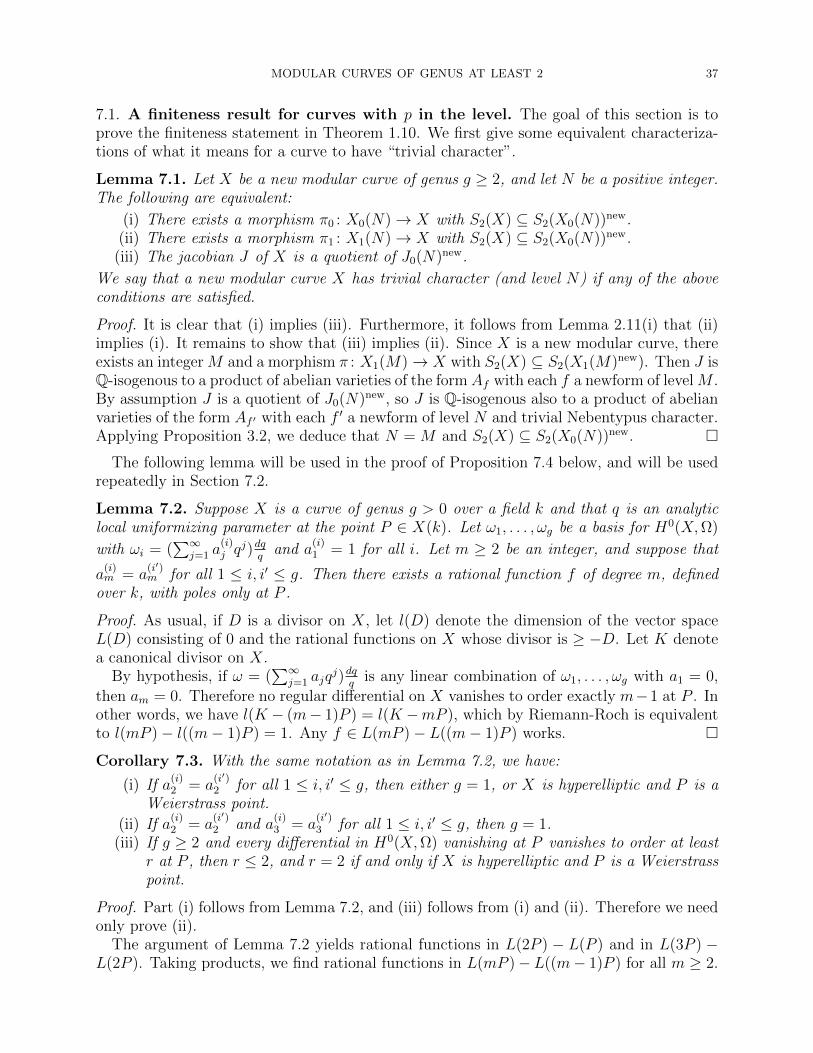
MODULAR CURVES OF GENUS AT LEAST 2 37
7.1. A finiteness result for curves with p in the level. The goal of this section is toprove the finiteness statement in Theorem 1.10. We first give some equivalent characteriza-tions of what it means for a curve to have “trivial character”.
Lemma 7.1. Let X be a new modular curve of genus g ≥ 2, and let N be a positive integer.The following are equivalent:
(i) There exists a morphism π0 : X0(N)→ X with S2(X) ⊆ S2(X0(N))new.(ii) There exists a morphism π1 : X1(N)→ X with S2(X) ⊆ S2(X0(N))new.
(iii) The jacobian J of X is a quotient of J0(N)new.
We say that a new modular curve X has trivial character (and level N) if any of the aboveconditions are satisfied.
Proof. It is clear that (i) implies (iii). Furthermore, it follows from Lemma 2.11(i) that (ii)implies (i). It remains to show that (iii) implies (ii). Since X is a new modular curve, thereexists an integer M and a morphism π : X1(M)→ X with S2(X) ⊆ S2(X1(M)new). Then J isQ-isogenous to a product of abelian varieties of the form Af with each f a newform of levelM .By assumption J is a quotient of J0(N)new, so J is Q-isogenous also to a product of abelianvarieties of the form Af ′ with each f ′ a newform of level N and trivial Nebentypus character.Applying Proposition 3.2, we deduce that N = M and S2(X) ⊆ S2(X0(N))new.
The following lemma will be used in the proof of Proposition 7.4 below, and will be usedrepeatedly in Section 7.2.
Lemma 7.2. Suppose X is a curve of genus g > 0 over a field k and that q is an analyticlocal uniformizing parameter at the point P ∈ X(k). Let ω1, . . . , ωg be a basis for H0(X,Ω)
with ωi = (∑∞
j=1 a(i)j q
j)dqq
and a(i)1 = 1 for all i. Let m ≥ 2 be an integer, and suppose that
a(i)m = a
(i′)m for all 1 ≤ i, i′ ≤ g. Then there exists a rational function f of degree m, defined
over k, with poles only at P .
Proof. As usual, if D is a divisor on X, let l(D) denote the dimension of the vector spaceL(D) consisting of 0 and the rational functions on X whose divisor is ≥ −D. Let K denotea canonical divisor on X.
By hypothesis, if ω = (∑∞
j=1 ajqj)dq
qis any linear combination of ω1, . . . , ωg with a1 = 0,
then am = 0. Therefore no regular differential on X vanishes to order exactly m−1 at P . Inother words, we have l(K − (m− 1)P ) = l(K −mP ), which by Riemann-Roch is equivalentto l(mP )− l((m− 1)P ) = 1. Any f ∈ L(mP )− L((m− 1)P ) works.
Corollary 7.3. With the same notation as in Lemma 7.2, we have:
(i) If a(i)2 = a
(i′)2 for all 1 ≤ i, i′ ≤ g, then either g = 1, or X is hyperelliptic and P is a
Weierstrass point.
(ii) If a(i)2 = a
(i′)2 and a
(i)3 = a
(i′)3 for all 1 ≤ i, i′ ≤ g, then g = 1.
(iii) If g ≥ 2 and every differential in H0(X,Ω) vanishing at P vanishes to order at leastr at P , then r ≤ 2, and r = 2 if and only if X is hyperelliptic and P is a Weierstrasspoint.
Proof. Part (i) follows from Lemma 7.2, and (iii) follows from (i) and (ii). Therefore we needonly prove (ii).
The argument of Lemma 7.2 yields rational functions in L(2P ) − L(P ) and in L(3P ) −L(2P ). Taking products, we find rational functions in L(mP )− L((m− 1)P ) for all m ≥ 2.
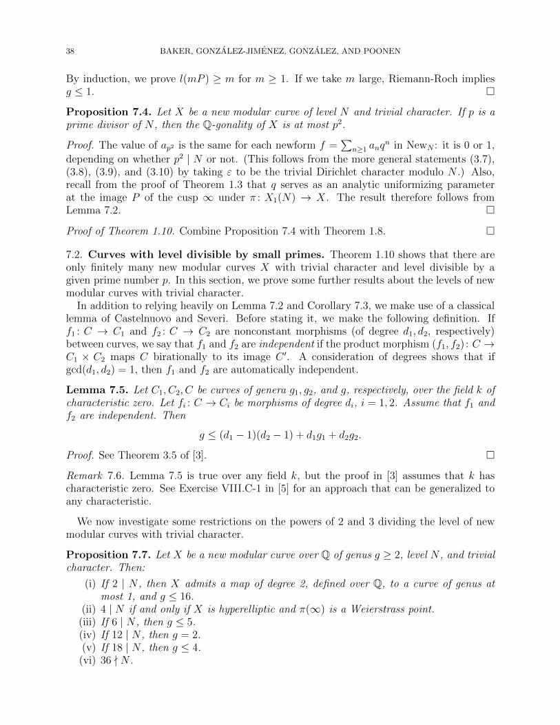
38 BAKER, GONZALEZ-JIMENEZ, GONZALEZ, AND POONEN
By induction, we prove l(mP ) ≥ m for m ≥ 1. If we take m large, Riemann-Roch impliesg ≤ 1.
Proposition 7.4. Let X be a new modular curve of level N and trivial character. If p is aprime divisor of N , then the Q-gonality of X is at most p2.
Proof. The value of ap2 is the same for each newform f =∑
n≥1 anqn in NewN : it is 0 or 1,
depending on whether p2 | N or not. (This follows from the more general statements (3.7),(3.8), (3.9), and (3.10) by taking ε to be the trivial Dirichlet character modulo N .) Also,recall from the proof of Theorem 1.3 that q serves as an analytic uniformizing parameterat the image P of the cusp ∞ under π : X1(N) → X. The result therefore follows fromLemma 7.2.
Proof of Theorem 1.10. Combine Proposition 7.4 with Theorem 1.8.
7.2. Curves with level divisible by small primes. Theorem 1.10 shows that there areonly finitely many new modular curves X with trivial character and level divisible by agiven prime number p. In this section, we prove some further results about the levels of newmodular curves with trivial character.
In addition to relying heavily on Lemma 7.2 and Corollary 7.3, we make use of a classicallemma of Castelnuovo and Severi. Before stating it, we make the following definition. Iff1 : C → C1 and f2 : C → C2 are nonconstant morphisms (of degree d1, d2, respectively)between curves, we say that f1 and f2 are independent if the product morphism (f1, f2) : C →C1 × C2 maps C birationally to its image C ′. A consideration of degrees shows that ifgcd(d1, d2) = 1, then f1 and f2 are automatically independent.
Lemma 7.5. Let C1, C2, C be curves of genera g1, g2, and g, respectively, over the field k ofcharacteristic zero. Let fi : C → Ci be morphisms of degree di, i = 1, 2. Assume that f1 andf2 are independent. Then
g ≤ (d1 − 1)(d2 − 1) + d1g1 + d2g2.
Proof. See Theorem 3.5 of [3].
Remark 7.6. Lemma 7.5 is true over any field k, but the proof in [3] assumes that k hascharacteristic zero. See Exercise VIII.C-1 in [5] for an approach that can be generalized toany characteristic.
We now investigate some restrictions on the powers of 2 and 3 dividing the level of newmodular curves with trivial character.
Proposition 7.7. Let X be a new modular curve over Q of genus g ≥ 2, level N , and trivialcharacter. Then:
(i) If 2 | N , then X admits a map of degree 2, defined over Q, to a curve of genus atmost 1, and g ≤ 16.
(ii) 4 | N if and only if X is hyperelliptic and π(∞) is a Weierstrass point.(iii) If 6 | N , then g ≤ 5.(iv) If 12 | N , then g = 2.(v) If 18 | N , then g ≤ 4.
(vi) 36 - N .

MODULAR CURVES OF GENUS AT LEAST 2 39
Proof. Let f1, . . . , fg be a basis of newforms for Γ0(N) spanning S2(X).To prove (ii), first note that, as in the proof of Theorem 1.3, the map π is unramified at∞, so that q serves as an analytic uniformizing parameter at P := π(∞). If 4 | N , thena2(fi) = 0 for all i by (3.9), so it follows from Corollary 7.3 that X is hyperelliptic and P isa Weierstrass point. The other direction of (ii) is a special case of Proposition 6.7.
Before proving (i), note that if 2 | N , then Proposition 7.4 implies that the Q-gonality GQof X satisfies GQ ≤ 4. Remark 4.5 then implies that g ≤ 34. We seek to sharpen both ofthese statements.
If X is hyperelliptic, then Theorem 1.9(ii) implies g ≤ 10. Therefore we may suppose thatX is not hyperelliptic. We may then assume by (ii) that 4 - N , so that it makes sense toconsider the Atkin-Lehner involution W2 on X.
Let X ′ = X/W2, let P ′ be the image in X ′ of P under the natural map, and let f ′1, . . . , f′g′
be a basis of newforms spanning S2(X ′). Then since fi|W2 = −a2(fi)fi by (3.12), we havea2(f ′i) = −1 for all i. Therefore every regular differential on X ′ vanishing at P ′ vanishes toorder at least 2 at P ′. We claim that X ′ has genus 1. Indeed, if the genus of X ′ were at least2, then Corollary 7.3 would then imply that X ′ is hyperelliptic and that P ′ is a Weierstrasspoint, but then we find by applying (ii) to X ′ that 4 | N , contrary to what we just assumed.Also, X ′ cannot have genus 0 or else X would be hyperelliptic, contrary to assumption. ThusX ′ has genus 1 as claimed, and X is a degree 2 cover (over Q) of the elliptic curve X ′.
If 3 - N , then we have #X(F9) ≤ 2#X ′(F9) ≤ 2(9+1+2√
9) = 32. But also (3−1)(g−1) <#X(F9) by Lemma 3.25. Thus g ≤ 16.
Finally, if 3 | N , then the conclusion g ≤ 16 follows from the stronger conclusion of (iii)proved below.
To prove (v), we suppose that 18 | N . It follows by Theorem 1.9(ii) that ifX is hyperellipticthen g < 3. Thus by (i), we may assume that X is a double cover of an elliptic curve X ′.
Since 9 | N , we have a3(fi) = 0 for all i, so Lemma 7.2 implies that X is trigonal (i.e., Xadmits a degree 3 map to P1). It therefore follows from Lemma 7.5 that g ≤ 4.
To prove (iii), we may assume by (v) that 3 | N but 9 - N . As before, we may also assumethat 2 | N but 4 - N , that X is not hyperelliptic, and that X is a double cover of the ellipticcurve X ′ = X/W2.
Let wj(fi) denote the eigenvalue of Wj on the newform fi for j = 2, 3, 6 and i = 1, . . . , g.We have w2(fi) = −a2(fi), w3(fi) = −a3(fi), and w6(fi) = a6(fi) for all i. Let gj be thegenus of X/Wj (j = 2, 3, 6), so gj = # i | wj(fi) = +1 . Since X/W2 has genus 1, all thew2(fi)’s are equal to −1 except for one, which is equal to +1. Suppose that f is the newformon which W2 acts with eigenvalue +1. The identity w2w3 = w6 and the fact that the w2’sare +1,−1,−1,−1, . . . ,−1 implies that g3 + g6 is equal to either g − 1 or g + 1, dependingon whether f |W3 equals −f or +f . We consider these two cases separately.
Case 1: f |W3 = −f .If g3 ≥ 2, then X/W3 is a curve of genus at least 2 with all w2’s equal to −1, so as
before we would have 4 | N , contrary to assumption. Thus g3 ≤ 1. Similarly, g6 ≤ 1. Butg3 + g6 = g − 1, so g ≤ 3.
Case 2: f |W3 = f .In this case, we have g3 ≥ 1. Also f |W6 = f , so g6 ≥ 1. Assume first that g3 = 1. Then
w2(fj) = w3(fj) for all j, so a simple argument using Riemann-Roch (as in the proof of

40 BAKER, GONZALEZ-JIMENEZ, GONZALEZ, AND POONEN
Lemma 7.2) shows that there is a rational function on X in L(3P )−L(2P ). Since (as in theproof of Proposition 7.4) all a4’s are equal to +1, there is also a function in L(4P )−L(3P ).Taking products, we also find functions in L(mP )− L((m− 1)P ) for all m ≥ 6, so that theWeierstrass gap sequence at P is contained in 1, 2, 5. By Riemann-Roch, the gap sequenceat any point contains exactly g integers, so g ≤ 3.
Assume now that g6 = 1. Then w2(fj) = w6(fj) for all j, so w3(fj) = 1 for all j.Corollary 7.3 gives a function in L(3P )− L(2P ), and as before we deduce that g ≤ 3.
In the general case, we may apply the previous reasoning to X/W3, since (X/W3)/W6 is ofgenus 1 (its only newform is f). The conclusion is that g3 ≤ 3. Similarly, since (X/W6)/W3
has genus 1, we conclude that g6 ≤ 3. Since g3 + g6 = g + 1 in Case II, we have g ≤ 5 asdesired.
To prove (vi), suppose that 36 | N . Then a2(fi) = a3(fi) = 0 for all i. By the sameargument as in the proof of (ii), it follows that every differential on X vanishing at Pvanishes to order at least 3 at P , contradicting Corollary 7.3.
For (iv), assume 12 | N . Then X is hyperelliptic by part (ii). By Theorem 1.9(ii), itfollows that g = 2 as desired.
We can deduce stronger results if we assume furthermore that the jacobian of X is Q-simple.
Proposition 7.8. Let X be a new modular curve of genus g ≥ 2, level N , and trivialcharacter. Assume furthermore that the jacobian J of X is Q-simple. Then:
(i) If 2 | N , then 4 | N .(ii) 6 - N .
Proof. Let f1, . . . , fg as before be a basis of newforms for Γ0(N) spanning S2(X). Since Jis Q-simple, the fi’s are all Galois conjugates of one another. To prove (i), suppose 2 | Nbut 4 - N . Then a2(fi) = ±1 for all i. Since in particular a2(fi) ∈ Q, all the a2(fi)’smust be equal to one another. It follows by Corollary 7.3 that X is hyperelliptic and P is aWeierstrass point. But then 4 | N by Proposition 7.7(ii), contradicting our assumption.
To prove (ii), suppose that 6 | N . By (i) we have in fact that 12 | N . Also, we know byProposition 7.7(vi) that 36 - N . Therefore we have a2(fi) = 0 and a3(fi) = ±1 for all i. Asabove, it follows that all the a3(fi)’s are in fact equal, contradicting Corollary 7.3.
8. Examples and Pathologies
8.1. Examples of non-new hyperelliptic curves. We can construct non-new modularhyperelliptic curves from certain pairs of new modular hyperelliptic curves. For some lev-els, there exist at least two new modular hyperelliptic curves of level N such that it ispossible to take the same modular function x in both their equations. In other words,Q(x,
√P1(x),
√P2(x)) is a subfield of the function field of X1(N), where the two new mod-
ular curves are
CN,1 : y21 = P1(x) , CN,2 : y2
2 = P2(x).
Then Q(x,√P1(x)P2(x)) also is a subfield of the function field of X1(N), so y2 = P1(x)P2(x)
is a modular hyperelliptic curve C ′N dominated by X1(N). (If desired, one may discard square
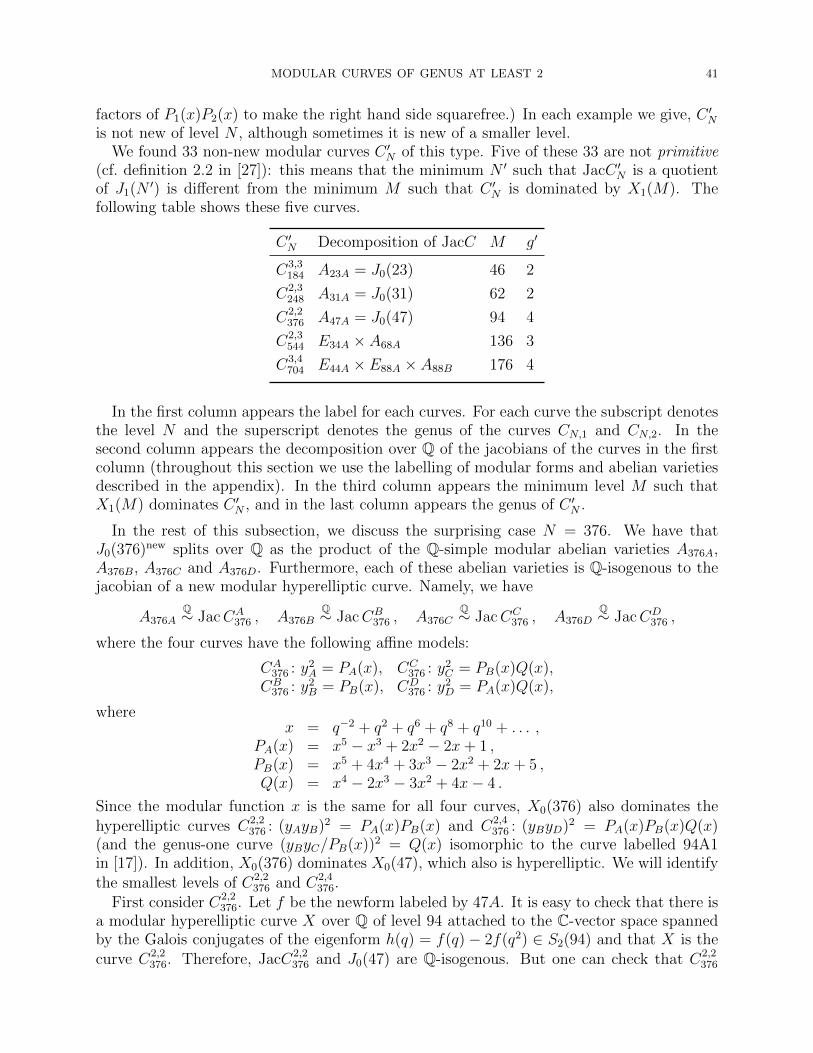
MODULAR CURVES OF GENUS AT LEAST 2 41
factors of P1(x)P2(x) to make the right hand side squarefree.) In each example we give, C ′Nis not new of level N , although sometimes it is new of a smaller level.
We found 33 non-new modular curves C ′N of this type. Five of these 33 are not primitive(cf. definition 2.2 in [27]): this means that the minimum N ′ such that JacC ′N is a quotientof J1(N ′) is different from the minimum M such that C ′N is dominated by X1(M). Thefollowing table shows these five curves.
C ′N Decomposition of JacC M g′
C3,3184 A23A = J0(23) 46 2
C2,3248 A31A = J0(31) 62 2
C2,2376 A47A = J0(47) 94 4
C2,3544 E34A × A68A 136 3
C3,4704 E44A × E88A × A88B 176 4
In the first column appears the label for each curves. For each curve the subscript denotesthe level N and the superscript denotes the genus of the curves CN,1 and CN,2. In thesecond column appears the decomposition over Q of the jacobians of the curves in the firstcolumn (throughout this section we use the labelling of modular forms and abelian varietiesdescribed in the appendix). In the third column appears the minimum level M such thatX1(M) dominates C ′N , and in the last column appears the genus of C ′N .
In the rest of this subsection, we discuss the surprising case N = 376. We have thatJ0(376)new splits over Q as the product of the Q-simple modular abelian varieties A376A,A376B, A376C and A376D. Furthermore, each of these abelian varieties is Q-isogenous to thejacobian of a new modular hyperelliptic curve. Namely, we have
A376AQ∼ JacCA
376 , A376BQ∼ JacCB
376 , A376CQ∼ JacCC
376 , A376DQ∼ JacCD
376 ,
where the four curves have the following affine models:
CA376 : y2
A = PA(x), CC376 : y2
C = PB(x)Q(x),CB
376 : y2B = PB(x), CD
376 : y2D = PA(x)Q(x),
wherex = q−2 + q2 + q6 + q8 + q10 + . . . ,
PA(x) = x5 − x3 + 2x2 − 2x+ 1 ,PB(x) = x5 + 4x4 + 3x3 − 2x2 + 2x+ 5 ,Q(x) = x4 − 2x3 − 3x2 + 4x− 4 .
Since the modular function x is the same for all four curves, X0(376) also dominates thehyperelliptic curves C2,2
376 : (yAyB)2 = PA(x)PB(x) and C2,4376 : (yByD)2 = PA(x)PB(x)Q(x)
(and the genus-one curve (yByC/PB(x))2 = Q(x) isomorphic to the curve labelled 94A1in [17]). In addition, X0(376) dominates X0(47), which also is hyperelliptic. We will identifythe smallest levels of C2,2
376 and C2,4376.
First consider C2,2376. Let f be the newform labeled by 47A. It is easy to check that there is
a modular hyperelliptic curve X over Q of level 94 attached to the C-vector space spannedby the Galois conjugates of the eigenform h(q) = f(q)− 2f(q2) ∈ S2(94) and that X is thecurve C2,2
376. Therefore, JacC2,2376 and J0(47) are Q-isogenous. But one can check that C2,2
376

42 BAKER, GONZALEZ-JIMENEZ, GONZALEZ, AND POONEN
and X0(47) are not Q-isomorphic. Hence 94 is the minimum level for C2,2376 while 47 is the
minimum level for its jacobian.
Now consider C2,4376. We compute that JacC2,4
376
Q∼ J0(47)×J0(94)new. More precisely, C2,2376 is
a non-new modular curve of minimum level 94: it is attached to the C-vector space generatedby the Galois conjugates of f(q) + 2f(q2) and g, where f is as above and g is the newformlabeled by 94B with dimA94B = 2. The curve C2,4
376 has genus 6, and its jacobian has onefactor in the new part and another in the old part.
Finally, we note that the highest genus yet found for a modular hyperelliptic curve is 7:the curve is given by the equation
C2,51664 : y2 = (x2 − 2x+ 2)(x2 + 2x+ 2)(x3 − x+ 2)(x3 − x− 2)(x6 + 2x4 + x2 + 4) ,
and has level N = 1664. Its jacobian splits as JacC2,51664
Q∼ E26A × A104B × A416F .
8.2. “Pathologies”. There are many statements about elliptic curve quotients of J1(N)that fail for modular curves of higher genus or for higher-dimensional abelian quotients ofJ1(N). We begin with a statement about abelian quotients.
Proposition 8.1. There exists an abelian variety A over Q such that the following statementis false: “If A is a quotient of J1(N) and N is the smallest integer with this property, andM is any other integer such that A is a quotient of J1(M), then N divides M .”
Proof. Take A = J0(22). One computes that there are no weight 2 newforms on Γ0(22), so
AQ∼ J0(11)2. Now A is not a quotient of J1(M) for any M prime to 11 because A has bad
reduction at 11, but A is also not a quotient of J1(11), since dim J1(11) = 1. Hence N = 22is the smallest integer for which A is a quotient of J1(N). On the other hand, (3.4) showsthat A is also a quotient of J1(11m) for any m ≥ 2.
Next we list a few false statements about modular curves.
Proposition 8.2. For each of the statements below, there is a curve X over Q of genusg ≥ 2 for which the statement is false. Let J = JacX.
(1) “If X is modular, then X is a new modular curve of some level.”(2) “If X is non-new modular of level N , then J is a quotient of J1(N)old.”(3) “If X is modular and N is the smallest level such that J is a quotient of J1(N) defined
over Q, then N is the smallest level of X.”(4) “If X is modular, then the smallest level of X and cond(J) are divisible by the same
rational primes.”(5) “If J is a Q-simple quotient of J1(N)new and X(Q) is nonempty, then X is a new
modular curve of level N .”
In fact, there exist infinitely many X over Q of genus 2 for which (5) fails.
Proof.(1) Let X = X1(p2) where p ≥ 11 is prime. It follows from an explicit formula for the
genus of X1(N) (see Example 9.1.6 of [20]) that 0 < 2g(X1(p)) < g(X1(p2)). Therefore,dim J1(p2)old = 2g(X1(p)) > 0 and dim J1(p2)new = g(X1(p2)) − dim J1(p2)old > 0. Now, byProposition 3.2 we obtain that if J1(p2)new is a quotient of J1(N)new over Q then N must bep2. Hence, X is not new for any level because J1(p2)old is not a quotient of J1(p2)new.
(2) Let X = X1(p2) for prime p ≥ 11 again. Then X is modular of level p2 and not newof any level, but JacX is not a quotient of J1(p2)old.

MODULAR CURVES OF GENUS AT LEAST 2 43
(3) Let X be the genus 4 curve C2,2376 constructed above. Then JacX is a quotient of J0(47)
(they are isogenous), but the smallest N for which X is modular of level N is 94.(4) Again let X = C2,2
376. Then cond(JacX) = 474 but the smallest N for which X ismodular of level N is 94. A simpler example is the genus 2 curve X = X0(22): thencond(JacX) = 112, but the smallest N for which X is modular of level N is 22.
(5) Let a ∈ Z− 0, and let Xa be the smooth projective model of the affine curve
y2 = x5 + ax3 − 4x
over Q of genus two. Then Xa(Q) 6= ∅, since (0, 0) ∈ Xa(Q). We will show that for infinitelymany values of a, the jacobian Ja := JacXa is a Q-simple quotient of some J1(N). It can bechecked that the group Aut(Xa) is isomorphic to D2·4 and is generated by the hyperellipticinvolution and the automorphisms u, v over Q(i), represented as in Lemma 6.12(1) by
Mu =
(0 1 + i
(1− i)/2 0
), Mv =
(i 00 −i
)(and e = detM). It can be checked that the
Galois action on Aut(Xa) corresponds to the case CC2 of section 3 of [13]. By Proposition
5.3 of [13], we obtain (End Ja) ⊗ Q ' Q(√
2). In particular, Ja is Q-simple. On the otherhand, the quotient Ea = Xa/u is the elliptic curve
y2 = x3 + 27(3a− 20i)x− 108(28 + 9ai)(1− i) ,whose j-invariant ja equals 64(3a − 20i)3(a − 4i)/(a2 + 16)2. Thus Ja is isogenous to theWeil restriction of Ea over Q. Solving ja = ja for a shows that ja is never real, so Ea doesnot have CM. Thus (End Ja) ⊗ Q is a real quadratic field, and the sign of the 2-cocycleattached to Ea by Ribet in [66] is trivial (see Theorem 5.4 of [62]). In particular, its localcomponent at 3 is trivial. For every nonzero a ∈ Z, Ea has good ordinary reduction at3, so Theorem 5.1 of [21] implies that Ea is modular (over Q(i)), so Ja is modular. SinceJa is Q-simple, it must be a quotient of J1(N)new for some N depending on a. Since ja isnonconstant, the family Xa is not isotrivial. (In fact, it can be proved that Xa and Xb areisomorphic over Q if and only if a = ±b.) Hence by Theorem 1.3, at most finitely manyof the Xa can be new modular curves. (In fact, Xa is a new modular curve exactly fora = ±1,±2,±3,±4,±5,±7,±8,±10,±22.)
Question 8.3. Is there a curve analogue of Proposition 8.1? More precisely, does there exista curve X dominated by some X1(N), but such that the set of such N for X are not allmultiples of the smallest N?
9. Curves dominated by Fermat curves
Here we prove an analogue of Conjecture 1.1 for Fermat curves. Let k be a field ofcharacteristic zero and let N ≥ 1. The N th Fermat curve XN,k is the smooth plane curveover k given by the homogeneous equation xN + yN = zN in P2
k. Our goal in this section isto prove the following.
Theorem 9.1. For each field k of characteristic zero, and integer g ≥ 2, the set of genus-gcurves over k dominated by XN,k for some N ≥ 1 is finite. If k is a number field or Q, thenthe set is also computable.
Let JN denote the jacobian of XN,k. For each M |N , there is a morphism ψN,M : XN,k →XM,k mapping (x : y : z) to (xN/M : yN/M : zN/M). Define JN,old =
∑M |N ψ
∗N,MJM , and
JnewN = JN/JN,old. We may consider XM,k as the quotient of XN,k by a Gk-stable subgroup

44 BAKER, GONZALEZ-JIMENEZ, GONZALEZ, AND POONEN
ΓN,M ⊆ Aut(XN,k). If we decompose the space H0(XN,k,Ω) into characters of ΓN,1, andgroup those for which a particular divisor M is the smallest M for which ΓN,M acts trivially,then we see that JN is k-isogenous to
∏M |N J
newM .
Lemma 9.2. If N > 180, then each k-simple quotient of JnewN has dimension at least φ(N)/8,
where φ(N) := #(Z/NZ)∗.
Proof. We may assume k = C. According to Theorem 1.3 of [4], JnewN ∼
∏AS, where each
AS is an abelian variety of dimension φ(N)/2, and S ranges over the elements of a certainfinite set Σ. Moreover, if N is not in an explicit finite set of natural numbers (whose largestelement is 180), then Theorem 0.2 of [4] shows that for each S ∈ Σ, AS = BWS
S , where BS isa simple abelian variety and WS ≤ 4. The result follows.
Lemma 9.3. There exists a function M = M(g) such that the following holds: If k is a fieldof characteristic zero, and X is a curve of genus g ≥ 2 over k dominated by XN,k for someN ≥ 1, then X is dominated also by XM ′,k for some M ′ ≤M .
Proof. Choose m > 180 such that φ(n)/8 > g for all n > m. Let M = m!. Suppose X isa curve of genus g ≥ 2 over k dominated by XN,k for some N ≥ 1. Let M ′ = gcd(M,N).By Lemma 9.2, the composition JacX → JN → Jnew
m′ is trivial for each m′|N greater thanm, so the image of JacX → JN is contained in an abelian subvariety of JN isogenousto∏
m′|N,m′≤m Jnewm′ , which in turn is contained in the image of JM ′ → JN . Considering
differentials and applying Proposition 2.11(i), we find that the morphism XN,k → X factorsthrough XM ′,k.
Proof of Theorem 9.1. Use Lemma 9.3, and then apply Theorem 5.7 (our de Franchis-SeveriTheorem) to XM ′,k for each M ′ ≤ M(g) to obtain a finite list of curves dominated byFermat curves over k, guaranteed to contain all those of genus g. If we now assume that kis a number field or Q, then this list is also computable. To eliminate curves of genus not g,and to eliminate possible redundancy, apply parts (1) and (3) of Lemma 5.1.
Remark 9.4.
(i) If k is a number field, we can obtain finiteness and computability also for dominatedcurves of genus ≤ 1 in Theorem 9.1. This follows from Remark 5.9: the genus-1isomorphism problem is not a problem here, because each dominated curve has arational point, thanks to the point (1 : 0 : 1) on each XN,k.
(ii) The natural analogue of Theorem 9.1 for bounded gonality is false. In affine coor-dinates, (x, y) 7→ (xy, yN) defines a dominant morphism from xN + yN = 1 to thehyperelliptic curve uN = v(1 − v). This gives infinitely many Fermat-dominatedcurves of gonality 2. These curves are even new, if N is prime. Perhaps the failure ofthe gonality result is not surprising, since in contrast with Theorem 4.3, the gonalityof high-degree smooth plane curves is small compared to the genus.
Question 9.5. Are there finiteness results for curves over Q of fixed genus g ≥ 2 that aredominated by curves in some other families, such as the family of Shimura curves associatedto orders in a fixed or varying indefinite quaternion algebra over Q?
Appendix
Labeling. We use a deterministic procedure to label newforms, and in particular to fix anordering of (Galois conjugacy classes of) newforms having a given level and Nebentypus. An

MODULAR CURVES OF GENUS AT LEAST 2 45
ordering was introduced by J. Cremona in [17] in the case of trivial Nebentypus and weight 2and generalized by W. A. Stein in [71] to the case of weight greater than 2. We are going touse this last labeling for the case of weight 2 and arbitrary Nebentypus.
We will define a function mapping each newform f ∈⋃∞N=1 NewN to a label of the form
NXε (for example, 13A2), where N is the level of f , where X is a letter or string inA,B, . . . , Z,AA,BB, . . . and ε is (some encoding) of the Nebentypus of f . If ε = 1, weomit the subscript ε and use a label of the form NX (for example, 11A), and if the Fouriercoefficients of f are integers we will use the labeling in [17]. The labeling function will notbe injective: our definition will be such that if f has label NXε and σ ∈ GQ, then σf willhave label NXσ(ε), which could be the same as NXε, even if σf 6= f .
Two things must be explained: how is X constructed from f , and how is ε encoded?First we construct X. Fix N and ε. To f =
∑anq
n ∈ NewN ∩ S2(N, ε) associate theinfinite sequence of integers tf = (TrEf/Q a1,TrEf/Q a2, . . . ), where Ef is the number fieldQ(a1, a2, . . . ). Choose X ∈ A,B, . . . , Z,AA,BB, . . . according to the position of tf inthe set tg : g ∈ NewN ∩ S2(N, ε) sorted in increasing dictionary order. Notice that tfdetermines the Galois conjugacy class of f .
The encoding of Dirichlet characters we now describe was suggested by J. Quer. Supposeε : (Z/NZ)∗ → C∗ is a Dirichlet character. Let N =
∏pαnn be the prime-ordered factor-
ization. Then there exist unique εpn : (Z/pαnn Z)∗ → C∗ such that ε =∏εpn . If p is an
odd prime, let gp be the smallest positive integer that generates (Z/pα Z)∗, and if p = 2and α ≤ 2, let gp = −1; in these cases εp is determined by the integer ep ∈ [0, ϕ(pα))such that εp(gp) = e2πiep/ϕ(pα). If p = 2 and α > 2, then ε2 is determined by the integerse′2, e
′′2 ∈ [0, ϕ(2α)) such that ε2(−1) = e2πie′2/ϕ(2α) and ε2(5) = e2πie′′2/ϕ(2α), and we write
e2 = e′2, e′′2. (Note: here and in the next sentence, we use set notation although we meansequences.) Assuming that N is implicit, we denote ε by ep : p|N.
If f ∈ S2(N, ε) is a newform with label NXε, then ANXε will denote the correspondingmodular abelian variety Af , except that when dimAf = 1, we instead follow the labelingin [15] and use the letter E instead of A to denote the modular elliptic curve Af .
We give an example illustrating the above notation: the 2-dimensional space S2(13) splitsas S2(13, ε)⊕S2(13, ε−1), where ε = 2 is a Dirichlet character modulo 13 (of order 6), and
there is only one Galois conjugacy class of newforms of level 13. Thus J1(13)Q∼ A13A2 .
Each new modular hyperelliptic curve in our tables will be denoted CM1,...,Mm
NL1,...,Lnεwhere
N is the level, the Li and Mj are letters (or in one case, the string AA) indicating thesimple factors of the jacobian J of the curve, and ε is (the label of) a Dirichlet character(Z/NZ)∗ → C∗. More precisely, the notation indicates that J is isogenous to the product ofthe Q-simple modular abelian varieties with the following labels: ANMj
for each superscriptMj and ANLiε for each subscript Li. (It turns out that in all known cases, there is at mostone Galois conjugacy class of nontrivial characters ε involved.)
Tables. Table 4 shows the 64 new modular curves of genus two with jacobian not Q-simple.(The 149 new modular curves of genus two with Q-simple jacobian were already listedin [27].) Tables 5, 6 and 7 show the 30 new modular hyperelliptic curves of genus > 2with Q-simple jacobian, trivial character, and level ≤ 3000, grouped by their genus. Recallthat by Proposition 1.3 of [68], a new modular curve with Q-simple jacobian and nontrivial

46 BAKER, GONZALEZ-JIMENEZ, GONZALEZ, AND POONEN
character must have even genus; this explains why we may omit the hypothesis #D = 1 inTables 5 and 7.
Tables 8, 9 and 10 show the 40 new modular hyperelliptic curves that have genus > 2and level ≤ 2000 such that the jacobian is a quotient of J0(N)new that is not Q-simple.Table 11 shows the five curves with genus 3 and #D = 3. Table 12 contains all new modularhyperelliptic curves with 2 | #D, w /∈ D and genus 3 ≤ g ≤ 4. All of them have genus 3and their jacobians are neither Q-simple nor a Q-factor of J0(N)new. Table 13 contains theremaining curves with #D > 1 and level ≤ 569. These curves have #D = 2, 3 or 4.
Remark 9.6. By inspection, the first curve in Table 13, namely CA52A,B0,4
, has a degree-2
unramified cover that dominates y2 = x6 + 4x5 + 6x4 + 2x3 +x2 + 2x+ 1, which is a equationfor X1(13). The fourth curve, CC
208A,D0,0,4, similarly has a degree-2 unramified cover that
dominates X1(13). The second and third curves in Table 13, namely C160A,E1,0,1 and
C160B,F 1,0,1 , have degree-2 unramified covers dominating y2 = p(x) and y2 = −p(−x),
respectively, where p(x) = (x− 1)(x2− 2x+ 2)(x2−x− 1); the latter two curves are the newmodular curves C160,C and C160,D of genus 2 from [27]. We do not have a good explanationfor this phenomenon.
Table 4: Not Q-simple, g = 2
C : y2 = F (x)
CA,B26 : y2 = x6 + 4x5 − 12x4 − 114x3 − 308x2 − 384x− 191
CA,B37 : y2 = x6 − 4x5 − 40x4 + 348x3 − 1072x2 + 1532x− 860
CA,B50 : y2 = x6 + 2x5 − 5x4 − 30x3 − 55x2 − 48x− 16
CA,B54 : y2 = x6 − 34x3 + 1
CA,B56 : y2 = x5 + 6x4 − 45x3 − 490x2 − 1503x− 1564
CA,B58 : y2 = x6 − 2x5 + 11x4 − 22x3 + 21x2 − 12x+ 4
CA,B66 : y2 = x6 + 2x5 − 5x4 − 22x3 − 31x2 − 24x− 8
CA,B80 : y2 = x5 + 2x4 − 26x3 − 132x2 − 231x− 142
CA,B84 : y2 = x5 + 4x4 − 25x3 − 172x2 − 339x− 222
CA,B90 : y2 = x6 − 18x3 + 1
CA,B91 : y2 = x6 + 2x5 − x4 − 8x3 − x2 + 2x+ 1
CA,B96 : y2 = x5 − 34x3 + x
CA,C112 : y2 = x5 − 2x4 + 10x3 − 16x2 + 21x− 14
CA,B112 : y2 = x5 − 6x4 − 45x3 + 490x2 − 1503x+ 1564
CB,D128 : y2 = x5 − 24x3 + 16x
CA,C128 : y2 = x5 + 24x3 + 16x
CA,C138 : y2 = x6 + 8x4 + 6x3 + 8x2 + 1
CB,D142 : y2 = x6 − 2x5 − 5x4 + 18x3 − 19x2 + 12x− 4
CA,B160 : y2 = x5 + 12x3 + 16x

MODULAR CURVES OF GENUS AT LEAST 2 47
C : y2 = F (x)
CA,D162 : y2 = x6 + 14x3 + 1
CB,C162 : y2 = x6 − 10x3 + 1
CC,D184 : y2 = x5 − 10x3 − 15x2 − 9x− 7
CA,C189 : y2 = x6 − 12x4 + 36x3 − 48x2 + 36x− 12
CA,B189 : y2 = x6 − 12x4 + 12x3 + 24x2 − 36x+ 12
CC,D192 : y2 = x5 − 14x3 + x
CB,D192 : y2 = x5 + 4x4 − 6x3 − 58x2 − 111x− 70
CA,C192 : y2 = x5 − 4x4 − 6x3 + 58x2 − 111x+ 70
CA,B192 : y2 = x5 + 34x3 + x
CC,E200 : y2 = x5 − 10x3 − 15x2 + 8
CC,D240 : y2 = x5 − 2x4 + 6x3 − 13x2 + 12x− 4
CA,D256 : y2 = x5 + 16x
CA,B264 : y2 = x5 + 2x4 − 6x3 − 23x2 − 24x− 8
CB,C312 : y2 = x5 − 2x4 − x3 + 8x2 − 9x+ 3
CA,C320 : y2 = x5 − 2x4 − 2x3 − 2x2 + x
CD,E320 : y2 = x5 − 12x3 + 16x
CB,F320 : y2 = x5 + 2x4 − 2x3 + 2x2 + x
CA,F336 : y2 = x5 − 4x4 − 25x3 + 172x2 − 339x+ 222
CA,G368 : y2 = x5 − 10x3 + 15x2 − 9x+ 7
CA,D384 : y2 = x5 + 10x3 + x
CB,C384 : y2 = x5 − 10x3 + x
CB,E400 : y2 = x5 − 25x2 + 20x− 4
CA,H400 : y2 = x5 − 10x3 + 15x2 − 8
CA,F405 : y2 = x6 − 12x4 + 28x3 − 24x2 + 12x− 4
CB,F405 : y2 = x6 − 12x4 + 20x3 − 12x+ 4
CA,D448 : y2 = x5 − 2x4 + 10x3 − 2x2 + x
CB,G448 : y2 = x5 + 2x4 + 10x3 + 2x2 + x
CB,C480 : y2 = x5 + 2x4 − 4x3 − 17x2 − 18x− 6
CB,G480 : y2 = x5 − 7x3 + x
CA,G480 : y2 = x5 − 2x4 − 4x3 + 17x2 − 18x+ 6
CA,D528 : y2 = x5 − 2x4 − 6x3 + 23x2 − 24x+ 8
CB,C544 : y2 = x5 − 9x3 + 16x
CC,D624 : y2 = x5 + 2x4 − x3 − 8x2 − 9x− 3
CA,G672 : y2 = x5 + 5x3 + x

48 BAKER, GONZALEZ-JIMENEZ, GONZALEZ, AND POONEN
C : y2 = F (x)
CA,E760 : y2 = x5 + 3x3 + 14x2 + 15x+ 5
CD,F768 : y2 = x5 − 4x3 + x
CB,H768 : y2 = x5 + 4x3 + x
CA,F960 : y2 = x5 + 7x3 + x
CL,N1088 : y2 = x5 + 9x3 + 16x
CC,F1344 : y2 = x5 − 5x3 + x
CB,D1520 : y2 = x5 + 3x3 − 14x2 + 15x− 5
CF,G1664 : y2 = x5 − 2x4 + x3 + 2x− 4
CO,S1664 : y2 = x5 + 2x4 + x3 + 2x+ 4
CA,E2208 : y2 = x5 + 2x4 + 8x3 + 19x2 + 18x+ 6
CG,I2208 : y2 = x5 − 2x4 + 8x3 − 19x2 + 18x− 6
Table 5: Q-simple, g = 3, N ≤ 3000
C : y2 = F (x)
CA41 : y2 = x8 + 4x7 − 8x6 − 66x5 − 120x4 − 56x3 + 53x2 + 36x− 16
CA95 : y2 = (x4 + x3 − 6x2 − 10x− 5)(x4 + x3 − 2x2 + 2x− 1)
CC152 : y2 = x(x3 − 2x2 − 7x− 8)(x3 + 4x2 + 4x+ 4)
CE248 : y2 = (x3 + x− 1)(x4 − 2x3 − 3x2 − 4x+ 4)
CA284 : y2 = x7 + 4x6 + 5x5 + x4 − 3x3 − 2x2 + 1
CB284 : y2 = x7 − 7x5 − 11x4 + 5x3 + 18x2 + 4x− 11
CG304 : y2 = x(x3 − 4x2 + 4x− 4)(x3 + 2x2 − 7x+ 8)
CJ496 : y2 = (x3 + x+ 1)(x4 + 2x3 − 3x2 + 4x+ 4)
CI544 : y2 = (x+ 1)(x2 + x− 4)(x4 − x2 − 4)
CJ544 : y2 = (x− 1)(x2 − x− 4)(x4 − x2 − 4)
CI896 : y2 = (x− 2)(x2 + 2x− 1)(x4 − 2x2 − 7)
CK896 : y2 = (x+ 2)(x2 − 2x− 1)(x4 − 2x2 − 7)
CG1136 : y2 = x7 − 7x5 + 11x4 + 5x3 − 18x2 + 4x+ 11
CJ1136 : y2 = x7 − 4x6 + 5x5 − x4 − 3x3 + 2x2 − 1
Table 6: Q-simple, g = 4, #D = 1, N ≤ 3000
C : y2 = F (x)
CA47 : y2 = (x5 − 5x3 − 20x2 − 24x− 19)(x5 + 4x4 + 7x3 + 8x2 + 4x+ 1)
CA119 : y2 = (x5 − 2x4 + 3x3 − 6x2 − 7)(x5 + 2x4 + 3x3 + 6x2 + 4x+ 1)

MODULAR CURVES OF GENUS AT LEAST 2 49
C : y2 = F (x)
CA164 : y2 = x(x8 + 4x7 − 8x6 − 66x5 − 120x4 − 56x3 + 53x2 + 36x− 16)
CC376 : y2 = (x4 − 2x3 − 3x2 + 4x− 4)(x5 + 4x4 + 3x3 − 2x2 + 2x+ 5)
CD376 : y2 = (x4 − 2x3 − 3x2 + 4x− 4)(x5 − x3 + 2x2 − 2x+ 1)
CF416 : y2 = x(x2 + 4)(x3 − 2x2 + x− 4)(x3 + 2x2 + x+ 4)
CG512 : y2 = x(x4 − 4x2 − 4)(x4 + 4x2 − 4)
CI656 : y2 = x(x8 − 4x7 − 8x6 + 66x5 − 120x4 + 56x3 + 53x2 − 36x− 16)
CG752 : y2 = (x4 + 2x3 − 3x2 − 4x− 4)(x5 − x3 − 2x2 − 2x− 1)
CI752 : y2 = (x4 + 2x3 − 3x2 − 4x− 4)(x5 − 4x4 + 3x3 + 2x2 + 2x− 5)
CP832 : y2 = x(x+ 2)(x− 2)(x6 + 2x4 − 15x2 + 16)
CW1216 : y2 = (x3 − 2x+ 2)(x6 + 2x4 − 7x2 + 8)
CX1216 : y2 = (x3 − 2x− 2)(x6 + 2x4 − 7x2 + 8)
Table 7: Q-simple, g = 5, N ≤ 3000
C : y2 = F (x)
CA59 : y2 = (x9 + 2x8 − 4x7 − 21x6 − 44x5 − 60x4 − 61x3 − 46x2 − 24x− 11)
(x3 + 2x2 + 1)
CY1664 : y2 = (x2 + 2x+ 2)(x3 − x+ 2)(x6 + 2x4 + x2 + 4)
CAA1664 : y2 = (x2 − 2x+ 2)(x3 − x− 2)(x6 + 2x4 + x2 + 4)
Table 8: Not Q-simple, g = 3, #D = 1, N ≤ 2000
C : y2 = F (x)
CA,B35 : y2 = (x2 + 3x+ 1)(x6 + x5 − 10x4 − 39x3 − 62x2 − 51x− 19)
CA,B39 : y2 = (x4 − 3x3 − 4x2 − 2x− 1)(x4 + 5x3 + 8x2 + 6x+ 3)
CA,B88 : y2 = (x− 2)(x3 − 2x2 + 4x− 4)(x3 + 2x2 − 4x+ 8)
CA,B104 : y2 = (x+ 2)(x6 + 4x5 − 12x4 − 114x3 − 308x2 − 384x− 191)
CA,B,C116 : y2 = (x+ 2)(x6 + 2x5 − 17x4 − 66x3 − 83x2 − 32x− 4)
CA,B,D128 : y2 = (x− 2)(x2 − 2x+ 2)(x4 − 12x2 + 32x− 28)
CB,C,D128 : y2 = (x+ 2)(x2 + 2x+ 2)(x4 − 12x2 − 32x− 28)
CA,C160 : y2 = (x− 2)(x2 + 2x− 7)(x4 − 4x3 + 10x2 − 20x+ 17)
CB,C160 : y2 = (x+ 2)(x2 − 2x− 7)(x4 + 4x3 + 10x2 + 20x+ 17)
CA,D176 : y2 = (x+ 2)(x3 − 2x2 − 4x− 8)(x3 + 2x2 + 4x+ 4)
CB,E184 : y2 = (x− 1)(x3 − 2x2 + 3x− 1)(x3 + x2 − x+ 7)
CA,C,D184 : y2 = (x− 1)(x6 − x5 + 4x4 − x3 + 2x2 + 2x+ 1)

50 BAKER, GONZALEZ-JIMENEZ, GONZALEZ, AND POONEN
C : y2 = F (x)
CB,C196 : y2 = (x3 + 2x2 − x− 1)(x4 − 2x3 − 9x2 + 10x− 3)
CB,E208 : y2 = (x− 2)(x6 − 4x5 − 12x4 + 114x3 − 308x2 + 384x− 191)
CA,D224 : y2 = x(x− 1)(x+ 1)(x4 − 6x2 + 16x− 7)
CB,C224 : y2 = x(x− 1)(x+ 1)(x4 − 6x2 − 16x− 7)
CB,D248 : y2 = (x3 + 4x2 + 5x+ 3)(x4 − 2x3 − 3x2 − 4x+ 4)
CB,E256 : y2 = x(x2 + 2)(x4 + 12x2 + 4)
CC,E256 : y2 = x(x2 − 4x+ 2)(x2 − 2)(x2 + 4x+ 2)
CA,D280 : y2 = (x− 1)(x6 − x5 + 7x3 − 16x2 + 15x− 5)
CC,I368 : y2 = (x+ 1)(x3 − x2 − x− 7)(x3 + 2x2 + 3x+ 1)
CA,D,G368 : y2 = (x+ 1)(x6 + x5 + 4x4 + x3 + 2x2 − 2x+ 1)
CA,E416 : y2 = x(x6 − 2x5 − 2x4 + 2x2 − 2x− 1)
CB,C416 : y2 = x(x6 + 2x5 − 2x4 + 2x2 + 2x− 1)
CD,E,F464 : y2 = (x− 2)(x6 − 2x5 − 17x4 + 66x3 − 83x2 + 32x− 4)
CC,G496 : y2 = (x3 − 4x2 + 5x− 3)(x4 + 2x3 − 3x2 + 4x+ 4)
CA,G560 : y2 = (x+ 1)(x6 + x5 − 7x3 − 16x2 − 15x− 5)
CC,K640 : y2 = x(x2 − 2x− 1)(x4 + 2x3 − 2x+ 1)
CG,I640 : y2 = x(x2 + 2x− 1)(x4 − 2x3 + 2x+ 1)
CB,N704 : y2 = x(x3 − 4x+ 4)(x3 + 2x2 − 2)
CC,O704 : y2 = x(x3 − 2x2 + 2)(x3 − 4x− 4)
CG,M784 : y2 = (x3 − 2x2 − x+ 1)(x4 + 2x3 − 9x2 − 10x− 3)
Table 9: Not Q-simple, g = 4, #D = 1, N ≤ 2000
C : y2 = F (x)
CC,D224 : y2 = x(x4 − 2x3 − 5x2 − 2x+ 1)(x4 + 2x3 − 5x2 + 2x+ 1)
CB,C236 : y2 = x9 + 2x8 − 4x7 − 21x6 − 44x5 − 60x4 − 61x3 − 46x2 − 24x− 11
CB,F,H368 : y2 = (x3 − x2 − x− 7)(x6 + x5 + 4x4 + x3 + 2x2 − 2x+ 1)
CI,J448 : y2 = x(x8 + 14x6 + 19x4 + 14x2 + 1)
CD,E,M704 : y2 = (x3 − 4x− 4)(x3 − 4x+ 4)(x3 + 2x2 − 2)
CF,I,P704 : y2 = (x3 − 2x2 + 2)(x3 − 4x− 4)(x3 − 4x+ 4)
CJ,L944 : y2 = x9 − 2x8 − 4x7 + 21x6 − 44x5 + 60x4 − 61x3 + 46x2 − 24x+ 11

MODULAR CURVES OF GENUS AT LEAST 2 51
Table 10: Not Q-simple, g = 6, #D = 1, N ≤ 2000
C : y2 = F (x)
CA,B71 : y2 = (x7 − 7x5 − 11x4 + 5x3 + 18x2 + 4x− 11)
(x7 + 4x6 + 5x5 + x4 − 3x3 − 2x2 + 1)
Table 11: g = 3, #D = 3
C : y2 = F (x)
CA21A0,2
: y2 = (x2 − x+ 1)(x6 + x5 − 6x4 − 3x3 + 14x2 − 7x+ 1)
CA36A0,2
: y2 = (x+ 1)(x+ 2)(x2 + 3x+ 3)(x3 − 9x− 9)
CA72A0,0,2
: y2 = x(x+ 1)(x2 + x+ 1)(x3 − 3x− 1)
CA144A0,0,2
: y2 = (x− 2)(x− 1)(x2 − 3x+ 3)(x3 − 9x+ 9)
CB144B0,0,2
: y2 = (x− 1)x(x2 − x+ 1)(x3 − 3x+ 1)
Table 12: g = 3, 2 | #D, w 6∈ D
C : y2 = F (x)
CA40A0,0,2
: y2 = x(x+ 1)(x+ 2)(x2 − 2x− 4)(x2 + 3x+ 1)
CA48A1,0,1
: y2 = (x+ 1)(x2 − 2x− 2)(x2 + x+ 1)(x2 + 2x+ 2)
CA64A0,8
: y2 = x(x− 1)(x+ 1)(x2 − 2x− 1)(x2 + 2x− 1)
CA80A0,0,2
: y2 = x(x− 1)(x− 2)(x2 − 3x+ 1)(x2 + 2x− 4)
CB80A0,0,2
: y2 = (x+ 1)(x2 − x− 1)(x4 + 4x2 + 8x+ 4)
CB128A0,16
: y2 = (x− 2)(x2 − 2x− 1)(x4 − 6x2 − 16x+ 41)
CD128A0,16
: y2 = (x+ 2)(x2 + 2x− 1)(x4 − 6x2 + 16x+ 41)
Table 13: g ≥ 4, #D > 1, N ≤ 569
C : y2 = F (x)
CA52A,B0,4
: y2 = x(x+ 1)(x3 − x2 − 4x− 1)(x6 + 4x5 + 6x4 + 2x3 + x2 + 2x+ 1)
C160A,E1,0,1 : y2 = (x− 1)(x2 − 2x+ 2)(x2 − x− 1)(x4 − 8x+ 8)
C160B,F 1,0,1 : y2 = (x+ 1)(x2 + 2x+ 2)(x2 + x− 1)(x4 + 8x+ 8)
CC208A,D0,0,4
: y2 = x(x− 1)(x3 + x2 − 4x+ 1)(x6 − 4x5 + 6x4 − 2x3 + x2 − 2x+ 1)
C512D0,64 : y2 = x(x8 + 24x4 + 16)

52 BAKER, GONZALEZ-JIMENEZ, GONZALEZ, AND POONEN
Acknowledgements
We thank Dinakar Ramakrishnan and Ken Ribet for discussing Proposition 3.2 with us.The proof of Theorem 5.7 grew out of discussions with Matthias Aschenbrenner, BrianConrad, Tom Graber, Tom Scanlon, and Jason Starr. We thank also Paul Gunnells, SorinPopescu, Xavier-Francois Roblot, William Stein and Tonghai Yang for suggesting references.Finally we thank a referee for an especially helpful report.
References
[1] Shreeram S. Abhyankar and Chanderjit L. Bajaj. Automatic parameterization of rational curves andsurfaces. III. Algebraic plane curves. Comput. Aided Geom. Design, 5(4):309–321, 1988.
[2] Dan Abramovich. A linear lower bound on the gonality of modular curves. Internat. Math. Res. Notices,(20):1005–1011, 1996.
[3] Robert D. M. Accola. Topics in the theory of Riemann surfaces. Springer-Verlag, Berlin, 1994.[4] Noboru Aoki. Simple factors of the Jacobian of a Fermat curve and the Picard number of a product of
Fermat curves. Amer. J. Math., 113(5):779–833, 1991.[5] E. Arbarello, M. Cornalba, P. A. Griffiths, and J. Harris. Geometry of algebraic curves. Vol. I. Springer-
Verlag, New York, 1985.[6] A. O. L. Atkin and Wen Ch’ing Winnie Li. Twists of newforms and pseudo-eigenvalues of W -operators.
Invent. Math., 48(3):221–243, 1978.[7] Lev A. Borisov, Paul E. Gunnells, and Sorin Popescu. Elliptic functions and equations of modular
curves. Math. Ann., 321(3):553–568, 2001.[8] Wieb Bosma, John Cannon, and Catherine Playoust. The Magma algebra system. I. The user language.
J. Symbolic Comput., 24(3-4):235–265, 1997. Computational algebra and number theory (London, 1993),homepage at http://magma.maths.usyd.edu.au/magma/ .
[9] Rolf Brandt and Henning Stichtenoth. Die Automorphismengruppen hyperelliptischer Kurven.Manuscripta Math., 55(1):83–92, 1986.
[10] Christophe Breuil, Brian Conrad, Fred Diamond, and Richard Taylor. On the modularity of ellipticcurves over Q: wild 3-adic exercises. J. Amer. Math. Soc., 14(4):843–939, 2001.
[11] E. Bujalance, J. M. Gamboa, and G. Gromadzki. The full automorphism groups of hyperelliptic Riemannsurfaces. Manuscripta Math., 79(3-4):267–282, 1993.
[12] Henri Carayol. Sur les representations l-adiques associees aux formes modulaires de Hilbert. Ann. Sci.
Ecole Norm. Sup. (4), 19(3):409–468, 1986.[13] G. Cardona and J. Quer. Curves of genus 2 with group of automorphisms isomorphic to D8 or D12.
Preprint, 2002.[14] Henri Cohen. Advanced topics in computational number theory, volume 193 of Graduate Texts in Math-
ematics. Springer-Verlag, New York, 2000.[15] J. E. Cremona. Elliptic curve data. 21 June 2004,
http://www.maths.nott.ac.uk/personal/jec/ftp/data/INDEX.html.[16] J. E. Cremona. Modular symbols for Γ1(N) and elliptic curves with everywhere good reduction. Math.
Proc. Cambridge Philos. Soc., 111(2):199–218, 1992.[17] J. E. Cremona. Algorithms for modular elliptic curves. Cambridge University Press, Cambridge, second
edition, 1997.[18] Mario Daberkow. On computations in Kummer extensions. Computational algebra and number theory
(Milwaukee, WI, 1996). J. Symbolic Comput., 31 (1–2):113–131, 2001.
[19] Pierre Deligne. La conjecture de Weil. I. Inst. Hautes Etudes Sci. Publ. Math., (43):273–307, 1974.[20] Fred Diamond and John Im. Modular forms and modular curves. In Seminar on Fermat’s Last Theorem
(Toronto, ON, 1993–1994), pages 39–133. Amer. Math. Soc., Providence, RI, 1995.[21] Jordan S. Ellenberg and Chris Skinner. On the modularity of Q-curves. Duke Math. J., 109(1):97–122,
2001.[22] Gerd Faltings. Finiteness theorems for abelian varieties over number fields. In Arithmetic geometry
(Storrs, Conn., 1984), pages 9–27. Springer, New York, 1986. Translated from the German original[Invent. Math., 73(3): 349–366, 1983; ibid. 75(2): 381, 1984] by Edward Shipz.

MODULAR CURVES OF GENUS AT LEAST 2 53
[23] Masahiro Furumoto and Yuji Hasegawa. Hyperelliptic quotients of modular curves X0(N). Tokyo J.Math., 22(1):105–125, 1999.
[24] Steven D. Galbraith. Rational points on X+0 (p). Experiment. Math., 8(4):311–318, 1999.
[25] David Goldschmidt. Algebraic Functions and Projective Curves. Springer-Verlag, New York, 2002.[26] J. Gonzalez. Equations of hyperelliptic modular curves. Ann. Inst. Fourier (Grenoble), 41(4):779–795,
1991.[27] E. Gonzalez-Jimenez and J. Gonzalez. Modular curves of genus 2. Math. Comp., 72(241):397–418, 2003.[28] Andrew Granville. ABC allows us to count squarefrees. Internat. Math. Res. Notices, (19):991–1009,
1998.[29] Georges Gras. Class field theory. From theory to practice. Springer Monographs in Mathematics.
Springer-Verlag, Berlin, 2003. Translated from the French manuscript by Henri Cohen.[30] Yuji Hasegawa. Hyperelliptic modular curves X∗
0 (N). Acta Arith., 81(4):369–385, 1997.[31] Yuji Hasegawa and Ki-ichiro Hashimoto. Hyperelliptic modular curves X∗
0 (N) with square-free levels.Acta Arith., 77(2):179–193, 1996.
[32] Yuji Hasegawa and Mahoro Shimura. Trigonal modular curves. Acta Arith., 88(2):129–140, 1999.
[33] Yuji Hasegawa and Mahoro Shimura. Trigonal modular curves X+d0 (N). Proc. Japan Acad. Ser. A Math.
Sci., 75(9):172–175, 1999.[34] Yuji Hasegawa and Mahoro Shimura. Trigonal modular curves X∗
0 (N). Proc. Japan Acad. Ser. A Math.Sci., 76(6):83–86, 2000.
[35] Grete Hermann. Die Frage der endlich vielen Schritte in der Theorie der Polynomideale. Math. Ann.,95:736–788, 1926.
[36] Florian Hess. An algorithm for computing isomorphisms of algebraic function fields. In AlgorithmicNumber Theory: 6th International Symposium, ANTS-VI, Burlington, VT, USA, June 13-18, 2004.Proceedings, volume 3076 of Lecture Notes in Comput. Sci., pages 263–271. Springer, Berlin, 2004.
[37] John E. Hopcroft and Jeffrey D. Ullman. Introduction to automata theory, languages, and computation.Addison-Wesley Publishing Co., Reading, Mass., 1979. Addison-Wesley Series in Computer Science.
[38] Dale Husemoller. Elliptic curves. Springer-Verlag, New York, 1987. With an appendix by Ruth Lawrence.[39] Jun-ichi Igusa. Kroneckerian model of fields of elliptic modular functions. Amer. J. Math., 81:561–577,
1959.[40] N. Ishii and F. Momose. Hyperelliptic modular curves. Tsukuba J. Math., 15(2):413–423, 1991.[41] E. Kani. Abelian subvarieties and the Shimura construction. Preprint, September 2004.
http://www.mast.queensu.ca/~kani/papers/absub4.pdf.[42] E. Kani. Endomorphisms of Jacobians of modular curves. Preprint, August 2004.
http://www.mast.queensu.ca/~kani/papers/endos2.pdf.[43] Nicholas M. Katz. p-adic interpolation of real analytic Eisenstein series. Ann. of Math. (2), 104(3):459–
571, 1976.[44] Henry H. Kim. Functoriality for the exterior square of GL4 and the symmetric fourth of GL2. J. Amer.
Math. Soc., 16(1):139–183 (electronic), 2003. With appendix 1 by Dinakar Ramakrishnan and appendix2 by Kim and Peter Sarnak.
[45] Felix Klein. Uber die Transformation elfter Ordnung der elliptischen Funktionen. Math. Ann., 15, 1879.reprinted in Ges. Math. Abh., Bd. III, art. LXXXVI, pp. 140–168.
[46] Peter George Kluit. Hecke operators on Γ∗(N) and their traces. Vrije Universiteit te Amsterdam, Am-sterdam, 1979. With a computer-aided study of low genus X∗(N), Dissertation, Vrije Universiteit,Amsterdam, 1979, With a Dutch summary.
[47] Serge Lang. Fundamentals of Diophantine geometry. Springer-Verlag, New York, 1983.[48] H. W. Lenstra, Jr. Algorithms in algebraic number theory. Bull. Amer. Math. Soc. (N.S.), 26(2):211–
244, 1992.[49] Wen Ch’ing Winnie Li. Newforms and functional equations. Math. Ann., 212:285–315, 1975.[50] Qing Liu and Dino Lorenzini. Models of curves and finite covers. Compositio Math., 118(1):61–102,
1999.[51] Paul Lockhart, Michael Rosen, and Joseph H. Silverman. An upper bound for the conductor of an
abelian variety. J. Algebraic Geom., 2(4):569–601, 1993.[52] Ju. I. Manin. Parabolic points and zeta functions of modular curves. Izv. Akad. Nauk SSSR Ser. Mat.,
36:19–66, 1972.

54 BAKER, GONZALEZ-JIMENEZ, GONZALEZ, AND POONEN
[53] David Marker. Model theory. An introduction. Volume 217 of Graduate Texts in Mathematics. Springer-Verlag, New York, 2002.
[54] Loıc Merel. Universal Fourier expansions of modular forms. In On Artin’s conjecture for odd 2-dimensional representations, volume 1585 of Lecture Notes in Math., pages 59–94. Springer, Berlin,1994.
[55] J.-F. Mestre. Corps euclidiens, unites exceptionnelles et courbes elliptiques. J. Number Theory,13(2):123–137, 1981.
[56] J. S. Milne. Abelian varieties. In Arithmetic geometry (Storrs, Conn., 1984), pages 103–150. Springer,New York, 1986.
[57] J. S. Milne. Jacobian varieties. In Arithmetic geometry (Storrs, Conn., 1984), pages 167–212. Springer,New York, 1986.
[58] Naoki Murabayashi. On normal forms of modular curves of genus 2. Osaka J. Math., 29(2):405–418,1992.
[59] A. Nerode. A decision method for p-adic integral zeros of diophantine equations. Bull. Amer. Math.Soc., 69:513–517, 1963.
[60] A. P. Ogg. Hyperelliptic modular curves. Bull. Soc. Math. France, 102:449–462, 1974.[61] Bjorn Poonen. Computational aspects of curves of genus at least 2. In Algorithmic number theory
(Talence, 1996), pages 283–306. Springer, Berlin, 1996.[62] Jordi Quer. Q-curves and abelian varieties of GL2-type. Proc. London Math. Soc. (3), 81(2):285–317,
2000.[63] Markus A. Reichert. Determination explicite des courbes elliptiques ayant un groupe de torsion non
trivial sur des corps de nombres quadratiques sur Q. In Seminar on number theory, 1983–1984 (Talence,1983/1984), pages Exp. No. 11, 33. Univ. Bordeaux I, Talence, 1984.
[64] Kenneth A. Ribet. Galois representations attached to eigenforms with Nebentypus. In Modular functionsof one variable, V (Proc. Second Internat. Conf., Univ. Bonn, Bonn, 1976), pages 17–51. Lecture Notesin Math., Vol. 601. Springer, Berlin, 1977.
[65] Kenneth A. Ribet. Twists of modular forms and endomorphisms of abelian varieties. Math. Ann.,253(1):43–62, 1980.
[66] Kenneth A. Ribet. Fields of definition of abelian varieties with real multiplication. In Arithmetic geom-etry (Tempe, AZ, 1993), pages 107–118. Amer. Math. Soc., Providence, RI, 1994.
[67] Goro Shimura. Introduction to the arithmetic theory of automorphic functions. Publications of the Math-ematical Society of Japan, No. 11. Iwanami Shoten, Publishers, Tokyo, 1971. Kano Memorial Lectures,No. 1.
[68] Goro Shimura. Class fields over real quadratic fields and Hecke operators. Ann. of Math. (2), 95:130–190,1972.
[69] Goro Shimura. On the factors of the jacobian variety of a modular function field. J. Math. Soc. Japan,25:523–544, 1973.
[70] Mahoro Shimura. Defining equations of modular curves X0(N). Tokyo J. Math., 18(2):443–456, 1995.[71] William Arthur Stein. Explicit approaches to modular abelian varieties. Ph. D. thesis, University of
California, Berkeley, 2000.[72] Alfred Tarski. A decision method for elementary algebra and geometry. University of California Press,
Berkeley and Los Angeles, Calif., 1951. 2nd ed.[73] Mark van Hoeij. Rational parametrizations of algebraic curves using a canonical divisor. J. Symbolic
Comput., 23(2-3):209–227, 1997. Parametric algebraic curves and applications (Albuquerque, NM, 1995).[74] Mark van Hoeij. An algorithm for computing the Weierstrass normal form of hyperelliptic curves, 2002.
arXiv:math.AG/0203130.[75] Jacques Velu. Courbes elliptiques munies d’un sous-groupe Z/nZ× µn. Bull. Soc. Math. France Mem.,
(57):5–152, 1978.

MODULAR CURVES OF GENUS AT LEAST 2 55
Department of Mathematics, University of Georgia, Athens, GA 30602-7403, USACurrent address: School of Mathematics, Georgia Institute of Technology, Atlanta, GA 30332-0160, USAE-mail address: [email protected]
School of Mathematical Sciences. University of Nottingham. University Park. Not-tingham, NG7 2RD, UK
Current address: Departamento de Analisis Economico: Economıa Cuantitativa, Facultad de CienciasEconomicas y Empresariales, Universidad Autonoma de Madrid, 28049 Madrid, Spain
E-mail address: [email protected]
Escola Universitaria Politecnica de Vilanova i la Geltru, Av. Vıctor Balaguer s/n, E-08800 Vilanova i la Geltru, Spain
E-mail address: [email protected]
Department of Mathematics, University of California, Berkeley, CA 94720-3840, USAE-mail address: [email protected]


![On the Finiteness Theorem of Siegel and Mahler › ~roquette › 1975... · [II] gave a proof for curves of genus g = 1, and he conjectured that the ... by the Riemann-Roth Theorem,](https://img.dokumen.tips/doc/110x75/5f0cfa5c7e708231d438125a/on-the-finiteness-theorem-of-siegel-and-mahler-a-roquette-a-1975-ii.jpg)