Finite Volume Method - TIFR CAMmath.tifrbng.res.in/~praveen/slides/annamalai.pdf · Finite Volume Method Praveen. C Computational and Theoretical Fluid Dynamics Division National

Praveen. C, CTFD Division, NAL, Bangalore First Prev Next Last Go Back Full Screen Close Quit

Finite Volume Method

Praveen. C

Computational and Theoretical Fluid Dynamics Division

National Aerospace Laboratories

Bangalore 560 017

email: [email protected]

Workshop on Advances in Computational Fluid Flow and Heat TransferAnnamalai University

October 17-18, 2005


Topics to be covered

1. Conservation Laws

2. Finite volume method

3. Types of finite volumes

4. Flux functions

5. Spatial discretization schemes

6. Higher order schemes

7. Boundary conditions

8. Accuracy and stability

9. Computational issues

10. References

Hyperbolic equations, Compressible flow, unstructured grid schemes


Conservation Laws and FVM

• Basic laws of physics are conservation laws - mass, momentum, energy

• Differential form∂U

∂t+

∂f

∂x+

∂g

∂y+

∂h

∂z= 0

U - conserved variables

f, g, h - flux vector

• Compressible flows - shocks and other discontinuities

• Classical solution may not exist

• Integral form (using divergence theorem)

∂

∂t

∫Ω

Udxdydz +

∮∂Ω

(fnx + gny + hnz)dS = 0

Rate of change of U in Ω = - (Net flux across the boundary of Ω)

⇓Starting point for finite volume method


• Discontinuities are a consequence of conservation laws

• Rankine-Hugoniot jump conditions [9, 10]

(fnx + gny + hnz)R − (fnx + gny + hnz)L = s(UR − UL)

n

U

U

L

RShock

• Solution satisfying integral form - weak solution

• Definition (Weak solution)

1. Satisfies the differential form in smooth regions

2. Satisfies jump condition across discontinuities

• Hyperbolic conservation laws - non-uniqueness

• Limit of a dissipative model: Navier-Stokes → Euler


• Entropy condition - second law of thermodynamics

• Entropy satisfying weak solution - unique (Kruzkov)

• Conservative scheme (FVM) - correct shock location (Warnecke)

• Useful for solving equations with discontinuous coefficients

• FVM can be applied on arbitrary grids - structured and unstructured














FVM in 1-D

• Divide computational domain [a, b] into N cells

a = x1/2 < x3/2 < . . . < xN+1/2 = b

Ci = [xi−1/2, xi+1/2]

Ci

hi−3/2 i−1/2 i+1/2 i+3/2i

• Conservation law for cell Ci

∂

∂t

∫ xi+1/2

xi−1/2

Udx + f (xi+1/2, t)− f (xi−1/2, t) = 0

• Cell average value

Ui(t) =1

hi

∫ xi+1/2

xi−1/2

U(x, t)dx


• Conservation law for cell Ci

hidUi

dt+ f (xi+1/2, t)− f (xi−1/2, t) = 0

U

U

i+1/2

i

i+1

• Riemann problem at each interface

• Numerical flux function (Godunov approach)

Fi+1/2(t) = F (Ui(t), Ui+1(t))

• Semi-discrete update equation (ODE system)

dUi

dt= − 1

hi[Fi+1/2(t)− Fi−1/2(t)]


• Method of lines approach

– Discretize in space

– Integrate the ODE system in time

• Explicit Euler scheme [ Uni ≈ U(xi, t

n) ]

Ui(tn+1)− Ui(t

n)

∆t= − 1

hi[Fi+1/2(t

n)− Fi−1/2(tn)]

⇓

Un+1i = Un

i −∆t

hi[F n

i+1/2 − F ni−1/2]

• Conservation: Telescopic collapse of fluxes∑i

hidUi

dt= −

∑i

[Fi+1/2(t)− Fi−1/2(t)]

= −[f (b, t)− f (a, t)]


Numerical Flux Function

• Simple averaging

Fi+1/2 = f ((Ui + Ui+1)/2) or Fi+1/2 = (fi + fi+1)/2

• Equivalent to central differencing

dUi

dt+

1

hi(fi+1 − fi−1) = 0 (unstable)

• Two approaches

1. Central differencing with artificial dissipation [13]

Fi+1/2 =1

2(fi + fi+1)− di+1/2

2. Upwind flux formula [9, 10, 13, 20, 22]

FVS: Fi+1/2 = f+(Ui) + f−(Ui+1)

FDS: Fi+1/2 =1

2(fi + fi+1)−

1

2[(∆f )−i+1/2 − (∆f )+i+1/2]


• Example: convection-diffusion equation

∂U

∂t+

∂f

∂x= 0, f = aU − ν

∂U

∂x

Fi+1/2 = aUi+1/2 − ν∂U

∂x

∣∣∣∣i+1/2

• Upwind definition of interfacial state

Ui+1/2 =

Ui if a ≥ 0

Ui+1 if a < 0

• Central-difference for viscous term

∂U

∂x

∣∣∣∣i+1/2

=Ui+1 − Ui

xi+1 − xi

• Upwind numerical flux

Fi+1/2 =1

2(aUi + aUi+1)−

|a|2

(Ui+1 − Ui)− νUi+1 − Ui

xi+1 − xi


Significance of conservative scheme

• Inviscid Burgers equation

∂U

∂t+

∂

∂x

(U 2

2

)= 0, f (U) =

U 2

2

• Rankine-Hugoniot condition

fR − fL = s(UR − UL) =⇒ s =1

2(UL + UR)

• Non-conservative form∂U

∂t+ U

∂U

∂x= 0

• Upwind scheme (assume U ≥ 0)

Un+1i − Un

i

∆t+ Un

i

Uni − Un

i−1

h= 0

or

Un+1i = Un

i −∆t

hUn

i (Uni − Un

i−1)


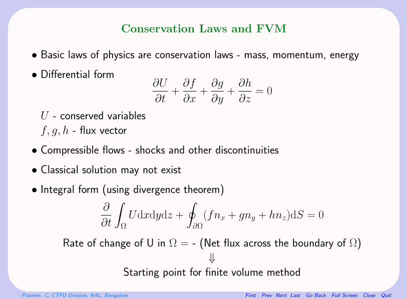
• Initial condition

U(x, 0) =

1 if x < 0

0 if x > 0

• Numerical solution

Uni = U o

i =⇒ stationary shock

• Exact solution (shock speed = 1/2)

U(x, t) =

1 if x < t/2

0 if x > t/2

• Conservation form from physical considerations

U∂U

∂t+ U

∂

∂x

(U 2

2

)= 0

or∂

∂t

(U 2

2

)+

∂

∂x

(U 3

3

)= 0

• Jump conditions not identical: s = 23

(U2

L+ULUR+U2R

UL+UR

)


Higher order scheme in 1-D

• Constant-in-cell representation

i−3/2 i−1/2 i+1/2 i+3/2

Ci−1

Ci+1

Ci

• First order accurate

|Ui − U(xi)| = O(h)

h = maxi

hi

• Reconstruction - evolution - projection



• Reconstruct the variation within a cell

i−3/2 i−1/2 i+1/2 i+3/2

Ci−1

Ci+1

Ci

Left state

Rightstate

• Linear reconstruction

U(x) = Ui + si(x− xi), x ∈ [xi−1/2, xi+1/2]

• Biased interpolant

ULi+1/2 = Ui + si(xi+1/2 − xi), UR

i+1/2 = Ui+1 + si+1(xi+1/2 − xi+1),


• Flux for higher order scheme

Fi+1/2 = F (Ui, Ui+1)

• Reconstruction variables

1. Conserved variables - conservative

2. Characteristic variables - better upwinding but costly

3. Primitive variables (ρ, u, p) - computationally cheap

• Unsteady flows - reconstruction must preserve conservation

1

hi

∫Ci

U(x)dx = Ui

• Gradients for reconstruction: backward, forward, central difference

si,b =Ui − Ui−1

xi − xi−1, si,f =

Ui+1 − Ui

xi+1 − xi, si,c =

Ui+1 − Ui−1

xi+1 − xi−1



Fi+1/2 = F (ULi+1/2, U

Ri+1/2)

• Reconstruction variables

1. Conserved variables - conservative

2. Characteristic variables - better upwinding but costly

3. Primitive variables (ρ, u, p) - computationally cheap

• Unsteady flows - reconstruction must preserve conservation

1

hi

∫Ci

U(x)dx = Ui

• Gradients for reconstruction: backward, forward, central difference

si,b =Ui − Ui−1

xi − xi−1, si,f =

Ui+1 − Ui

xi+1 − xi, si,c =

Ui+1 − Ui−1

xi+1 − xi−1


• Solution with discontinuity

1

1/2

i−1 i i+1


• Central-difference: Non-monotone reconstruction

1

1/2

i−1 i i+1

• Limited gradients [9, 12]

si = Limiter(si,b, si,f , si,c)


FVM in 2-D

• Divide computational domain into disjoint polygonal cells, Ω = ∪iCi

• Integral form for cell Ci

∂

∂t

∫Ci

Udxdy +

∮∂Ci

(fnx + gny)dS = 0

• Cell average value

Ui(t) =1

|Ci|

∫Ci

U(x, y, t)dxdy, |Ci| = area of Ci

• Cell connectivity: N(i) = j : Cj and Ci share a common face

Ci Ci


∮∂Ci

(fnx + gny)dS =∑

j∈N(i)

∫Ci∩Cj

(fnx + gny)dS

• Approximate flux integral by quadrature

C

n

C

i

j

ij

∫Ci∩Cj

(fnx + gny)dS ≈ Fij∆Sij

• Semi-discrete update equation

|Ci|dUi

dt= −

∑j∈N(i)

Fij∆Sij


• Numerical flux function

Fij = F (Ui, Uj, nij)

• Properties of flux function

1. Consistency

F (U,U, n) = f (U)nx + g(U)ny

2. Conservation

F (V, U,−n) = −F (U, V, n)

3. Continuity

‖F (UL, UR, n)− F (U,U, n)‖ ≤ C max (‖UL − U‖, ‖UR − U‖)

• Flux functions [10, 13, 20, 22]

– FVS: Steger-Warming, Van Leer, KFVS, AUSM

– FDS: Godunov, Roe, Engquist-Osher

• Integrate in time using a Runge-Kutta scheme [5, 12]


Grids and Finite Volumes

• Elements in 2-D

• Elements in 3-D


• Boundary layers - prism and hexahedra

• Cell-centered and vertex-centered scheme [5, 18, 21]

• Median (dual) cell

– join centroid to mid-point of sides

– well-defined for any triangulation

Centroid

Mid−point


• Voronoi cell

– join circum-center to mid-point of sides

– smooth area variation

– not defined for obtuse triangles

• Containment circle tessalation


Median and containment-circle tessalation


• Stretched triangles - median dual and containment-circle

• Containment-circle finite volume


• Turbulent flow over RAE2822 airfoil: vertex-centered scheme

Mach = 0.729, α = 2.31 deg, Re = 6.5 million



• Bi-linear reconstruction in cell Ci

U(x, y) = Ui + ai(x− xi) + bi(y − yi), (x, y) ∈ Ci

U

U L

R

C

C

i

j

• Define left/right states

UL = Ui + ai(xij − xi) + bi(yij − yi)

UR = Uj + aj(xij − xj) + bj(yij − yj)


Fij = F (UL, UR, nij)


• Gradient estimation using

1. Green-Gauss theorem

2. Least squares fitting

• Green-Gauss theorem ∫Ci

∇Udxdy =

∮∂Ci

UndS

• Approximate surface integral by quadrature

∇Ui ≈1

|Ci|∑face

∫face

UndS

• Face value

Uface =1

2(UL + UR)

• Non-uniform cells

Uface = αUL + (1− α)UR, α ∈ (0, 1)

• Accuracy can degrade for non-uniform grids [4, 6, 8, 14]


• Least-squares reconstruction [3, 5]

1

2

3

4

0

Uo + ao(xj − xo) + bo(yj − yo) = Uj, j = 1, 2, 3, 4

• Over-determined system of equations - solve by least-squares fit

min∑

j

[Uj − Uo − ao(xj − xo)− bo(yj − yo)]2, wrt ao, bo

ao =∑

j

αj(Uj − Uo), bo =∑

j

βj(Uj − Uo)


• Limited reconstruction

– Cell-centered: Min-max [3, 5], Venkatakrishnan [5], ENO-type [1, 14]

– Vertex-centered: edge-based limiter [17]

• Min-max limiter

Umin ≤ Uo + ao(xj − xo) + bo(yj − yo) ≤ Umax, j = 1, 2, 3, 4

(ao, bo)←− (φao, φbo), φ ∈ [0, 1]

– Very dissipative - smeared shocks

– Performance degrades on coarse grids

– Stalled convergence - limit cycle

– Useful for flows with large discontinuities

• Venkatakrishnan limiter

– Smooth modification of min-max limiter

– Better control - depends on cell size

– Better convergence properties


• Vertex-centered cell: Edge-based limiter

L R

i i+1i−1

i+2

UL = Ui +1

2Limiter

[(Ui+1 − Ui),

|PiPi+1||PiPi−1|

(Ui − Ui−1)

]• Using vertex-gradients

UL = Ui +1

2Limiter

[(Ui+1 − Ui), (~Pi+1 − ~Pi) · ∇Ui

]• Van-albada limiter

Limiter(a, b) =(a2 + ε)b + (b2 + ε)a

a2 + b2 + 2ε, ε 1


Higher order flux quadrature

U L1

U R1

U L2

U R2

C

C

i

j

• Quadratic reconstruction in cell Ci

U(x, y) = Ui + ai(x− xi) + bi(y − yi)

+ ci(x− xi)2 + di(x− xi)(y − yi) + ei(y − yi)

2

• 2-point Gauss quadrature for flux

Fij = ω1F (UL1 , UR

1 , nij) + ω2F (UL2 , UR

2 , nij)


Discretization of viscous flux

• Viscous terms

∇ · µ∇u

• Finite volume discretization∫Ci

(∇ · µ∇u)dV =

∮∂Ci

(µ∇u · n)dS

• Simple averaging

∇uij =1

2(∇ui +∇uj)

– Odd-even decoupling on quadrilateral/hexahedral cells

– Large stencil size

• 1-D case: ut = uxx

un+1i = un

i +∆t

2h(un

i−2 − 2uni + un

i+2)

• Correction for decoupling problem [5]


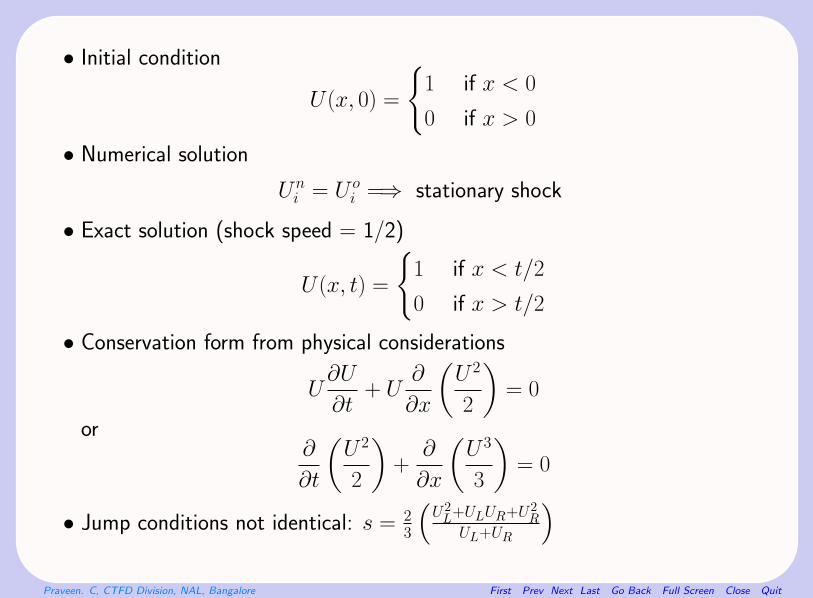
• Green-Gauss theorem for auxiliary volume

Face−centered volume

i

j

• Least-squares gradients

– Quadratic reconstruction: gradients and hessian [3]

– Face-centered least-squares

• Vertex-centered scheme

– Galerkin approximation on triangles/tetrahedra

– Nearest neighbour stencil


Turbulence models

• Reynolds-average Navier-Stokes equations - need turbulence models

• Differential equation based models: k − ε, k − ω, Spalart-Allmaras

• Turbulence quantities must remain positive

• Discretize using first order upwind finite volume method

Example: Spalart-Allmaras model∫Ci

∇ · (νu)dV ≈∑

j∈N(i)

[(uij · nij)+νi + (uij · nij)

−νj]∆Sij

(·)± =(·)± |(·)|

2, uij =

1

2(ui + uj)

• Coupled or de-coupled approach

• Stiffness problem - positivity preserving implicit methods


Boundary conditions

• Cell-centered approach

1. Ghost cell

2. Flux boundary condition

w

g

Boundary

Ghost cell

• Inviscid flow (slip flow - zero normal velocity)

ρg = ρw, pg = pw, ug = uw, vg = −vw

• Viscous flow (noslip flow - zero velocity)

ρg = ρw, pg = pw, ug = −uw, vg = −vw


• Boundary flux depends on pressure only

F (Uw, Ug, n) = function of p only

• Flux boundary condition

(~F · n)wall = p[0, nx, ny, 0]>

1. Extrapolate pressure from interior cells

2. Solve normal momentum equation [2]

• Vertex-centered approach - flux boundary condition

• Boundary cell in vertex-centered scheme


Accuracy and Stability

• FVM with linear reconstruction - second order accurate on uniform and

smooth grids

• On non-uniform grids =⇒ formally first order accurate

• Local truncation error not a good indicator of global error [22]

• r’th order reconstruction and ng Gaussian points for flux quadrature - accu-

racy is min(r, 2ng) [19]

• Semi-discrete scheme

dUi

dt=

∑j∈N(i)

aij(Uj − Ui), aij ≥ 0

• Local Extremum Diminishing (LED) property - maxima do not increase and

minima do not decrease (Jameson)


• If Ui is a local maximum =⇒ Uj − Ui ≤ 0

dUi

dt=

∑j∈N(i)

aij(Uj − Ui) ≤ 0 =⇒ Ui does not increase

• Fully discrete scheme

Un+1i = (1−∆t

∑j

aij)Uni +

∑j

aijUnj , ∆t ≤ 1∑

j aij

• Convex linear combination

minj∈N(i)

Unj ≤ Un+1

i ≤ maxj∈N(i)

Unj

• Prevents oscillations (Gibbs phenomenon) near discontinuities

• Stable in maximum norm

minj

Unj ≤ Un+1

i ≤ maxj

Unj

• Elliptic equations - discrete maximum principle

minj∈∂Ω

Uj ≤ Ui ≤ maxj∈∂Ω

Uj


Data structures and Programming

• Data structure for FVM

– Coordinates of vertices

– Indices of vertices forming each cell

• Cell-based updating

------------------------------------------------------

for cell = 1 to Ncell

FluxDiv = 0

for face = 1 to Nface(cell)

cellNeighbour = CellNeighbour(cell, face)

flux = NumFlux(cell, cellNeighbour)

FluxDiv += flux

end

Unew(cell) = Uold(cell) - dt*FluxDiv

end------------------------------------------------------


• Face-based updating

------------------------------------------------------

FluxDiv(:) = 0

for face = 1 to Nface

LeftCell = FaceCell(face,1)

RightCell = FaceCell(face,2)

flux = NumFlux(LeftCell, RightCell)

FluxDiv(LeftCell) += flux

FluxDiv(RightCell) -= flux

end

Unew(:) = Uold(:) - dt*FluxDiv(:)

------------------------------------------------------

• Flux computations reduced by half - speed-up of two

• Other geometric quantities - cell centroids, face areas, face normals, face

centroids


References

[1] Abgrall R., “On essentially non-oscillatory schemes on unstructured meshes:

analysis and implementation”, J. Comp. Phys., Vol. 114, pp. 45-58, 1994.

[2] Balakrishnan N. and Fernandez, G., “Wall Boundary Conditions for Inviscid

Compressible Flows on Unstructured Meshes”, Int. Jl. for Num. Methods in

Fluids, 28:1481-1501, 1998.

[3] Barth T. J., “Aspects of unstructured grids and solvers for the Euler and

NS equations”, Von Karman Institute Lecture Series, AGARD Publ. R-787,

1992.

[4] Barth T. J., “Recent developments in high order k-exact reconstruction on

unstructured meshes”, AIAA Paper 93-0668, 1993.

[5] Blazek J., Computational Fluid Dynamics: Principles and Applications, El-

sevier, 2004.


[6] Delanaye M., Geuzaine Ph. and Essers J. A., “Development and application

of quadratic reconstruction schemes for compressible flows on unstructured

adaptive grids”, AIAA-97-2120, 1997.

[7] Feistauer M., Felcman J. and Straskraba I., Mathematical and Computa-

tional Methods for Compressible Flow, Clarendon Press, Oxford, 2003.

[8] Frink N. T., “Upwind scheme for solving the Euler equations on unstructured

tetrahedral meshes”, AIAA J. 30(1), 70, 1992.

[9] Godlewski E. and Raviart P.-A., Hyperbolic Systems of Conservation Laws,

Paris, Ellipses, 1991.

[10] Godlewski E. and Raviart P.-A., Numerical Approximation of Hyperbolic

Systems of Conservation Laws, Springer, 1996.

[11] Carl Ollivier-Gooch and Michael Van Altena, “A high-order-accurate unstruc-

tured mesh finite-volume scheme for the advection-diffusion equation”, JCP,

181, 729-752, 2002.

[12] Hirsch Ch., Numerical Computation of Internal and External Flows, Vol. 1,

Wiley, 1988.


[13] Hirsch Ch., Numerical Computation of Internal and External Flows, Vol. 2,

Wiley, 1989.

[14] Jawahar and Kamath H., “A High-Resolution Procedure for Euler and Navier-

Stokes Computations on Unstructured Grids“, Journal of Computational

Physics, Vol. 164, No. 1, pp. 165-203, 2000

[15] Kallinderis Y. and Ahn H. T., “Incompressible Navier-Stokes method with

general hybrid meshes”, J. Comp. Phy., Vol. 210, pp. 75-108, 2005.

[16] LeVeque R. J., Finite Volume Methods for Hyperbolic Equations, Cambridge

University Press, 2002.

[17] Lohner R., Applied CFD Techniques: An Introduction based on FEM, Wiley.

[18] Mavriplis D. J., “Unstructured grid techniques”, Ann. Rev. Fluid Mech.,

29:473-514, 1997.

[19] Sonar Th., “Finite volume approximations on unstructured grids”, VKI Lec-

ture Notes.


[20] Toro E., Riemann Solvers and Numerical Methods for Fluid Dynamics,

Springer.

[21] Venkatakrishnan V, “Perspective on unstructured grid flow solvers”, AIAA

Journal, vol. 34, no. 3, 1996.

[22] Wesseling P., Principles of Computational Fluid Dynamics, Springer, 2001.

Thank YouThese slides can be downloaded from

http://pc.freeshell.org/pub/annamalai.pdf

Documents

Finite Volume Method - TIFR CAMmath.tifrbng.res.in/~praveen/slides/annamalai.pdf · Finite Volume Method Praveen. C Computational and Theoretical Fluid Dynamics Division National