Finite State Markov-chain Approximations to Highly

Persistent Processes∗

Karen A. Kopecky† Richard M. H. Suen‡

This Version: February 2010

Abstract

The Rouwenhorst method of approximating stationary AR(1) processes has been overlooked by

much of the literature despite having many desirable properties unmatched by other methods. In

particular, we prove that it can match the conditional and unconditional mean and variance, and the

first-order autocorrelation of any stationary AR(1) process. These properties makes the Rouwenhorst

method more reliable than others in approximating highly persistent processes and generating accurate

model solutions. To illustrate this, we compare the performances of the Rouwenhorst method and

four others in solving the stochastic growth model and an income fluctuation problem. We find that

(i) the choice of approximation method can have a large impact on the computed model solutions, and

(ii) the Rouwenhorst method is more robust than others with respect to variation in the persistence

of the process, the number of points used in the discrete approximation and the procedure used to

generate model statistics.

Keywords: Numerical Methods, Finite State Approximations

JEL classification: C63.

∗We thank Russell Cooper, Paul Klein, John Rust, and conference participants at the UCR Conference on BusinessCycles, CEF 2009 and the Workshop for Economists Working in Parallel for helpful comments and suggestions. We thankYundong Tu for excellent research assistance.

†Department of Economics, Social Science Center, Room 4701, The University of Western Ontario, London, Ontario,N6A 5C2, Canada. Email: kkopecky@uwo.ca.

‡Corresponding author. Department of Economics, Sproul Hall, University of California, Riverside CA 92521-0427.Email: richard.suen@ucr.edu. Tel.: (951) 827-1502. Fax: (951) 827-5685.

1 Introduction

In macroeconomic models, the exogenous stochastic process is typically assumed to follow a stationary

first-order autoregressive process. When solving these models numerically, the continuous-valued autore-

gressive process is usually replaced by a discrete state-space Markov chain. To this end, researchers typ-

ically employ the approximation method proposed by Tauchen (1986), or the quadrature-based method

developed in Tauchen and Hussey (1991). For AR(1) processes with low persistence, these methods

can produce highly accurate approximations. However, their performance deteriorates when the serial

correlation is very close to one.1 These findings raise concerns because macroeconomic studies typically

employ highly persistent processes. In particular, there are two main questions that await answers.

First, is there a more reliable technique to approximate highly persistent processes? Second, how does

the performance of these methods affect the computed solutions of macroeconomic models? In quanti-

tative studies, approximating the exogenous process is seldom an end in itself. Thus a more appropriate

metric for evaluating approximation methods would be their impact on the computed solutions of the

entire model. To the best of our knowledge, no existing studies have performed this kind of evaluation.

The current study is intended to fill this gap.

Regarding the first question, this paper re-examines a Markov-chain approximation method that

is first proposed in Rouwenhorst (1995). The main strength of this method is that it can match five

important statistics of any stationary AR(1) process, including the conditional and unconditional mean,

the conditional and unconditional variance, and the first-order autocorrelation. This property makes the

Rouwenhorst method more reliable than the other methods in approximating highly persistent processes.

The first contribution of this paper is to provide formal proofs of this and other results.2

Our second contribution is to compare the performances of five different approximation methods

in solving two common macroeconomic models. The methods under study include the Tauchen (1986)

method, the original Tauchen-Hussey method, a variation of this method proposed by Floden (2008a),

the Adda-Cooper (2003) method and the Rouwenhorst method. The first model that we consider is

the prototypical stochastic neoclassical growth model without leisure.3 The main evaluation criterion in1This weakness is acknowledged in the original papers. In Tauchen (1986, p.179), the author notes that “Experimentation

showed that the quality of the approximation remains good except when λ [the serial correlation] is very close to unity.” InTauchen and Hussey (1991), the authors note that for processes with high persistence, “adequate approximation requiressuccessively finer state spaces.”

2Some of the features of this method are briefly mentioned in Rouwenhorst (1995). But a formal proof of these resultsis still lacking.

3The same model is used in Taylor and Uhlig (1990) and the companion papers to illustrate and compare differentsolution methods. More recently, Aruoba et al. (2006) use the stochastic growth model, but with labor-leisure choice, tocompare different solution methods.

1

this application is the accuracy in approximating the business cycle moments generated by the model.

The second model that we consider is an income fluctuation problem. This problem is of interest

because it forms an integral part of the heterogeneous-agent models considered in Aiyagari (1994) and

Krusell and Smith (1998). There is now a large literature that uses these models to examine issues

in macroeconomics and finance. These models often contain highly persistent processes for individual

labor income risk. In some cases, the discretization method used for these processes may be crucial to

the validity of the final conclusions. For instance, when these models are used to analyze the welfare

implications of policy reforms or eliminating business cycles, the welfare gains or losses are usually quite

small.4 Thus an accurate approximation could ultimately result in the difference between a welfare gain

or loss. When solving the income fluctuation problem, the five methods are evaluated for their accuracy

in approximating the degree of inequality in consumption, income and assets. In both models, we use

two different approaches to compute the statistics of interest. In the baseline approach the statistics are

computed using an approximation to the stationary distribution. In the second approach, the statistics

are generated using Monte Carlo simulations.

For the stochastic growth model, regardless of which approach is taken, the choice of approximation

method has a large impact on the accuracy of the computed business cycle moments. Moreover, a method

that generates a good approximation for the AR(1) process also tends to yield accurate approximations

for the business cycle moments. The Rouwenhorst method has the best performance in this regard.

Furthermore, the high degree of accuracy of the Rouwenhorst method prevails even when a coarse state

space (with only five states for the exogenous shock) is used. The Tauchen (1986) method has the second

best performance, followed by Floden’s variation of the Tauchen-Hussey method. However, these two

methods require a much finer state space (at least 25 states) in order to produce the same precision

as the Rouwenhorst method. One interesting finding is that the baseline approach, coupled with the

Rouwenhorst method, performs as well as the simulation approach.

As for the income fluctuation problem, consistent with our previous findings, the methods which

generate good approximations for the AR(1) process tend to yield more accurate solutions under the

baseline approach. The Rouwenhorst method and Floden’s variation have the best performance in this

regard. However, the Rouwenhorst method is less sensitive to changes in the number of states in the

Markov chain. It is also the only method that produces very similar, yet relatively accurate, results

under both the baseline approach and the simulation approach.4See, for instance, Krusell et al. (2009) for a recent study that examines the welfare implications of eliminating business

cycles in this type of model.

2

In sum, our quantitative results have two main implications. First, the accuracy of the approximation

for the exogenous process can have a large impact on the computed solutions of macroeconomic models.

Thus caution must be taken when choosing an approximation method. Second, our results show that

the Rouwenhorst method is the most robust of the five methods considered with respect to the degree

of persistence of the AR(1) process, the coarseness of the discrete state space, and the approach used

to compute the statistics from the stationary distribution. The accuracies of model solutions computed

using the Tauchen (1986) method and the Tauchen-Hussey method, on the other hand, are both sensitive

to these choices. It is also worth noting that the performance of the Tauchen (1986) method is extremely

sensitive to the choice of a free parameter that determines the bounds on the state space of the discrete

process. This feature of the Tauchen (1986) method is overlooked by the existing studies.

The current study is related to Floden (2008a) and Lkhagvasuren and Galindev (2008). The objective

of Floden (2008a) is to compare the relative performance of various discretization methods in approxi-

mating stationary AR(1) processes. However, Floden does not consider the Rouwenhorst method, nor

does he consider the impact of the discretization procedure on the solutions of macroeconomic models.

The main objective of Lkhagvasuren and Galindev (2008) is to develop an approximation method for

vector autoregressive processes with correlated error terms. These authors show, through a few numer-

ical examples, that the Rouwenhorst method outperforms other methods in approximating moments of

univariate AR(1) processes. In contrast, this result is formally proved in the current study.

2 The Rouwenhorst Method

Consider the AR(1) process

zt = ρzt−1 + εt, (1)

where |ρ| < 1 and εt is a white noise process with variance σ2ε. The AR(1) process is covariance-stationary

with mean zero and variance σ2z = σ2

ε/(1− ρ2

). If, in addition, εt is normally distributed in each

period, then zt is also normally distributed. Rouwenhorst (1995) proposes a method to approximate this

stochastic process by a discrete state-space process yt. This involves constructing an N -state Markov

chain characterized by (i) a symmetric and evenly-spaced state space YN = y1, ..., yN , with y1 = −ψ

and yN = ψ, and (ii) a transition matrix ΘN . For any N ≥ 2, the transition matrix ΘN is determined

by two parameters, p, q ∈ (0, 1) , and is defined recursively as follows:

3

Step 1: When N = 2, define Θ2 as

Θ2 =

p 1− p

1− q q

.

Step 2: For N ≥ 3, construct the N -by-N matrix

p

ΘN−1 0

0′ 0

+ (1− p)

0 ΘN−1

0 0′

+ (1− q)

0′ 0

ΘN−1 0

+ q

0 0′

0 ΘN−1

,

where 0 is a (N − 1)-by-1 column vector of zeros.

Step 3: Divide all but the top and bottom rows by two so that the elements in each row sum to one.

The main objective of this section is to show formally that the Rouwenhorst method has a number

of desirable features unmatched by other methods. However, the matrix ΘN generated by the procedure

above is difficult to work with analytically. Thus, we begin our analysis by offering a new, analytically

tractable procedure for generating the Rouwenhorst matrix. The main advantage of this new procedure

is that it greatly simplifies the proofs of our analytical results.

2.1 Reconstructing the Rouwenhorst Matrix

For any p, q ∈ (0, 1) and for any integer N ≥ 2, define a system of polynomials as follows

Φ (t; N, i) ≡ [p + (1− p) t]N−i (1− q + qt)i−1 , (2)

for i = 1, 2, ..., N. Expanding the polynomials in (2) yields

Φ (t; N, i) =N∑

j=1

π(N)i,j tj−1, for i = 1, 2, ..., N. (3)

Define an N -by-N matrix ΠN =[π

(N)i,j

]using the coefficients in (3). The main result of this subsection

is Proposition 1 which states that the matrix ΠN is identical to the Rouwenhorst matrix ΘN for any

integer N ≥ 2. All proofs can be found in the Appendix.

Proposition 1 For any N ≥ 2 and for any p, q ∈ (0, 1) , the matrix ΠN defined above is identical to the

Rouwenhorst matrix ΘN generated by Steps 1-3.

4

Table 1: Selected Moments of the Markov ChainConditional Mean E(yt+1|yt = yi) (q − p) ψ + (p + q − 1) yi

Conditional Variance var(yt+1|yt = yi)4ψ2

(N−1)2[(N − i) (1− p) p + (i− 1) q (1− q)]

Unconditional Mean E(yt)(q−p)ψ2−(p+q)

Unconditional Second Moment E(y2

t

)ψ2

1− 4s (1− s) + 4s(1−s)

N−1

First-order Autocovariance Cov(yt, yt+1) (p + q − 1)var(yt)First-order Autocorrelation Corr(yt, yt+1) p + q − 1

2.2 Discrete State-Space Markov Chain

Consider a Markov chain yt with a symmetric and evenly-spaced state space YN = y1, ..., yN defined

over the interval [−ψ, ψ] . The transition matrix of the Markov chain is given by ΠN , which is a stochas-

tic matrix of non-zero entries.5 It follows immediately that the Markov chain has a unique invariant

distribution. This result is stated in Proposition 2.

Proposition 2 For any N ≥ 2, the Markov chain with state space YN and transition matrix ΠN has a

unique invariant distribution λ(N) =(λ

(N)1 , ..., λ

(N)N

), where λ

(N)i ≥ 0 and

∑Ni=1 λ

(N)i = 1.

Rouwenhorst mentions that in the symmetric case where p = q, the unique invariant distribution is

a binomial distribution with parameters N − 1 and 1/2. Our next result shows that the unique invariant

distribution is binomial for any p, q ∈ (0, 1) . Since the invariant distribution is unique, it can be solved

by the guess-and-verify method. Let s ≡ 1−q2−(p+q) ∈ (0, 1) . The guess for λ(N), represented by λ

(N), is a

binomial distribution with parameters N − 1 and 1− s. This means

λ(N)

i =(

N − 1i− 1

)sN−i (1− s)i−1 , for i = 1, 2, ..., N. (4)

It is easy to check that this is the actual solution when N = 2. The result for the general case is

established in Proposition 3.

Proposition 3 For any N ≥ 2, the invariant distribution of the Markov chain defined above is a

binomial distribution with parameters N − 1 and 1− s.

Equipped with the invariant distribution, one can derive the unconditional moments of the Markov

chain. Some of these moments are shown in Table 1.6

5See Lemma 2 in Kopecky and Suen (2009) for a formal proof of this statement.6The mathematical derivations of these results can be found in Kopecky and Suen (2009) Appendix B.

5

2.3 Approximating AR(1) Processes

The task at hand is to approximate a given stationary AR(1) process with an N -state Markov chain.7

Let zt be the stationary AR(1) process defined in (1). Conditional on the realization of zt−1, the

mean and variance of zt are given by ρzt−1 and σ2ε, respectively. Now define an N -state discrete Markov

process yt as in Section 2.2 with

p = q =1 + ρ

2and ψ =

√N − 1σz. (5)

Using the equations in Table 1, it is immediate to see that the resulting Markov chain has the same

unconditional mean, unconditional variance and first-order autocorrelation as zt . Suppose yt−1 = yi

for some yi in YN . The conditional mean and conditional variance of yt are given by

E (yt|yt−1 = yi) = ρyi and var (yt|yt−1 = yi) = σ2ε.

Thus yt also has the same conditional mean and conditional variance as zt .

Two remarks regarding this procedure are worth mentioning. First, under the Rouwenhorst method,

the approximate Markov chain is constructed using ρ and σ2ε alone. In particular, the transition matrix

ΠN is not a discretized version of the conditional distribution of zt. This is the fundamental difference

between this method and the ones proposed in Tauchen (1986) and Tauchen and Hussey (1991). Second,

the above procedure can be applied to any stationary AR(1) process, including those with very high

persistence. Thus, unlike the other two methods, the one proposed by Rouwenhorst can always match

the unconditional variance and the persistence of zt .

Since the invariant distribution of yt is a binomial distribution with mean zero and variance σ2y =

σ2ε/(1−ρ2), the standardized process yt/σy converges to the standard normal distribution as N goes to

infinity. Thus the Rouwenhorst method is particularly apt for approximating Gaussian AR(1) processes.

3 Evaluations

In this section we examine the performance of the Rouwenhorst method and four other discretization

methods in solving the stochastic growth model and the income fluctuation problem. For the stochastic7In this paper, we focus on univariate AR(1) processes only. For vector autoregressive processes, one can combine the

Rouwenhorst method with the decomposition method proposed in Lkhagvasuren and Galindev (2008). More specifically,these authors propose a method to decompose a multivariate process into a number of independent univariate processes.These independent processes can then be approximated using the Rouwenhorst method described below.

6

growth model, the main evaluation criterion is the accuracy in approximating the business cycle moments

generated by the model. For the income fluctuation problem, we focus on measures of inequality in

consumption, income and assets. The other methods under evaluation are described below.

Tauchen (1986) method Under this method, an evenly-spaced state space YN = y1, ..., yN is used

to construct the Markov chain yt, with yN = −y1 = Ωσz, where Ω is a positive real number and σz is

the standard deviation of the original AR(1) process. Let Φ be the probability distribution function for

the standard normal distribution. For any i = 1, ..., N, the transition probabilities of the Markov chain

are given by

πi,j = Φ(

yj − ρyi + h/2σε

),

for j = 1 and N, and

πi,j = Φ(

yj − ρyi + h/2σε

)− Φ

(yj − ρyi − h/2

σε

),

for j = 2, ..., N−1, where h is the step size between the grid points. It turns out that the performance of

this method is strongly affected by the choice of Ω. To the best of our knowledge, there is no established

rule for determining this parameter.8 In all the results reported below, Ω is calibrated such that the

standard deviation of yt matches the standard deviation of the AR(1) process. This gives the method

its best chance in approximating the AR(1) process.9

The Quadrature-Based Methods Under this class of methods, the elements of the state space

are determined by yi =√

2σxi, for i = 1, 2, ..., N, where xi are the Gauss-Hermite nodes defined on

[−∞,∞] . Letφj

be the corresponding Gauss-Hermite weights. The elements in the transition matrix

Π are then given by

πi,j =f

(yj |yi

)

f(yj |0

) wj

si,

where wj = φj/√

π, the function f (·|yi) is the density function for N(ρyi, σ

2), and

si =N∑

n=1

f (yn|yi)f (yn|0)

wn.

8Tauchen (1986) sets Ω = 3 without giving any justification. Floden (2008) sets Ω = 1.2 ln (N) . As explained in Section3.1, Floden’s choice of Ω is the main reason why he finds that the Tauchen (1986) method performs poorly in approximatinghighly persistent processes.

9We choose to target σz instead of ρ because, relative to σz, the persistence parameter ρ is well approximated underthis method for a range of values of Ω and degrees of persistence.

7

In Tauchen and Hussey (1991), the standard deviation σ is taken to be σε. In Floden (2008a), σ is a

weighted average of σz and σε. In particular, σ = ωσε + (1− ω) σz with ω = 0.5 + 0.25ρ.

The Adda-Cooper (2003) Method The first step of this method is to partition the real line into N

intervals. Formally, let In = [xn, xn+1] be the nth interval with x1 = −∞ and xN+1 = +∞. The cut-off

points xnNn=2 are the solutions of the following system of equations:

Φ(

xn+1

σz

)− Φ

(xn

σz

)=

1N

, for n = 1, 2, ..., N,

where Φ is the probability distribution function for the standard normal distribution. The nth element

in the state space is the mean value of the nth interval. For any i, j ∈ 1, 2, ..., N , the transition

probability πi,j is defined as the probability of moving from interval Ii to interval Ij in one period.

3.1 Stochastic Growth Model

Consider the planner’s problem in the stochastic growth model,

maxCt,Kt+1∞t=0

E0

[ ∞∑

t=0

βt log (Ct)

]

subject to

Ct + Kt+1 = exp (at) Kαt + (1− δ) Kt,

at+1 = ρat + εt+1, with ρ ∈ (0, 1) , (6)

Ct, Kt+1 ≥ 0, and K0 given, where Ct denotes consumption at time t, Kt denotes capital, At ≡ exp (at) is

the technological factor and εt+1 ∼ i.i.d. N(0, σ2

ε

). The parameter β ∈ (0, 1) is the subjective discount

factor, α ∈ (0, 1) is the share of capital income in total output and δ ∈ (0, 1] is the depreciation rate.

The Bellman equation for this problem is

V (K, a) = maxK′

log

(exp (a) Kα + (1− δ) K −K ′) + β

∫V

(K ′, a′

)dF

(a′|a)

, (7)

where F (·|a) is the distribution function of at+1 conditional on at = a.

8

Parameterization and Computation

Following King and Rebelo (1999), we use the following parameter values: α = 0.33, β = 0.984, δ = 0.025,

σε = 0.0072 and ρ = 0.979. Under this parameterization, the business cycle moments of interest do not

have closed-form solutions. Thus we first compute a highly accurate approximation of these moments.

To do this we use the Chebyshev parameterized expectation algorithm described in Christiano and Fisher

(2000) to compute the policy function.10 We then generate a sequence of at of length 50,010,000 using the

actual AR(1) process. The first 10,000 observations are discarded (the “burn-in”) and the rest are used

to compute the business cycle moments. The solutions obtained will be referred to as the “quasi-exact”

solutions of the model.

We then compute the business cycle moments using the discretization methods mentioned above.

First, the AR(1) process in (6) is replaced by a Markov chain with state space A = a1, ..., aN and

transition matrix Π = [πi,j ] . Next, we form an evenly-spaced grid for k ≡ ln K, represented by K =k1, ..., kM

. In the results reported below, we set M = 1, 000 and use three different values for N, namely

5, 10 and 25. The Bellman equation in (7) is then solved over the discrete state space S = K×A using

the value-function iteration method described in Tauchen (1990) and Burnside (1999). The outcome is

a discrete approximation to the policy function, denoted by

g(km, an

):(km, an

) ∈ S

.

The business cycle moments are then computed using two different approaches. Under the baseline

approach, an approximation to the stationary distribution of the state variables (k, a) is computed by

iterating on the equation

πlP = πl+1, (8)

where P is the transition matrix for (k, a) . The iterations proceed until the “distance” between successive

iterates, as measured by max∣∣∣πl − πl+1

∣∣∣ , is within the desired tolerance. The business cycle moments

are then derived using πl and the computed policy function g. Under the second approach, the business

cycle moments are generated using Monte Carlo simulations. First, we generate a common sequence of

at of length 5,010,000 using the actual AR(1) process with a burn-in period of 10,000. We then use the

computed policy function to construct a sequence of kt ≡ ln Kt. Linear interpolation is used to compute10Specifically, we compute the continuous shock version of the model using the Chebyshev parameterized expectation

approach and the Wright-William specification of the conditional expectation function. The conditional expectation functionis approximated by

∑Ni=1 θiCi(k, a), where Ci(k, a), i = 1, . . . , N are the elements of the set Ti1(φ(k))Ti2(ψ(a))|∑2

j=1 ij ≤n and θi, i = 1, . . . , N are the weights. The functions Tij for j = 1, 2 are the ith Chebyshev polynomials and φ and ψare linear mappings of [kmin, kmax] and [−3σ, 3σ] into the interval [−1, 1]. We set n = 12 so that N = 78 and we useM = 2, 916 quadrature nodes, 54 in each direction. Further increasing N and M results in a less than 1 percent change inall the business cycle moments computed. Following Christiano and Fisher (2000), the conditional expectation is computedusing 4-point Gauss-Hermite quadrature.

9

values of g (kt, at) for points not in the discrete state space S.

One major difference between these two approaches is the sources of the errors that they introduce.

While both methods suffer from errors in the computation of the policy function, under the baseline

approach, additional errors occur due to the discrete approximation of the stationary distribution. How-

ever, this approach does not suffer from the approximation errors due to linear interpolation and the

sampling errors generated by the simulation method.11

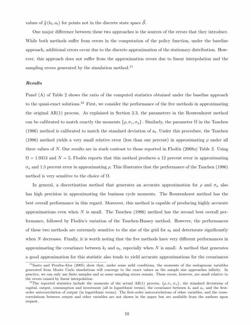
Results

Panel (A) of Table 2 shows the ratio of the computed statistics obtained under the baseline approach

to the quasi-exact solutions.12 First, we consider the performance of the five methods in approximating

the original AR(1) process. As explained in Section 2.3, the parameters in the Rouwenhorst method

can be calibrated to match exactly the moments ρ, σε, σa . Similarly, the parameter Ω in the Tauchen

(1986) method is calibrated to match the standard deviation of at. Under this procedure, the Tauchen

(1986) method yields a very small relative error (less than one percent) in approximating ρ under all

three values of N. Our results are in stark contrast to those reported in Floden (2008a) Table 2. Using

Ω = 1.9313 and N = 5, Floden reports that this method produces a 12 percent error in approximating

σa and 1.5 percent error in approximating ρ. This illustrates that the performance of the Tauchen (1986)

method is very sensitive to the choice of Ω.

In general, a discretization method that generates an accurate approximation for ρ and σa also

has high precision in approximating the business cycle moments. The Rouwenhorst method has the

best overall performance in this regard. Moreover, this method is capable of producing highly accurate

approximations even when N is small. The Tauchen (1986) method has the second best overall per-

formance, followed by Floden’s variation of the Tauchen-Hussey method. However, the performances

of these two methods are extremely sensitive to the size of the grid for at and deteriorate significantly

when N decreases. Finally, it is worth noting that the five methods have very different performances in

approximating the covariance between kt and at, especially when N is small. A method that generates

a good approximation for this statistic also tends to yield accurate approximations for the covariances11Santo and Peralta-Alva (2005) show that, under some mild conditions, the moments of the endogenous variables

generated from Monte Carlo simulations will converge to the exact values as the sample size approaches infinity. Inpractice, we can only use finite samples and so some sampling errors remain. These errors, however, are small relative tothe errors caused by linear interpolation.

12The reported statistics include the moments of the actual AR(1) process, ρ, σε, σa , the standard deviations ofcapital, output, consumption and investment (all in logarithmic terms), the covariance between kt and at, and the first-order autocorrelation of output (in logarithmic terms). The first-order autocorrelations of other variables, and the cross-correlations between output and other variables are not shown in the paper but are available from the authors uponrequest.

10

between yt and other endogenous variables. It is thus important to choose a method that can match this

statistic well. As the table shows, the Rouwenhorst method generates the most accurate approximation

of this covariance and, as a result, the rest of the business cycle moments.13

Panel (B) of Table 2 reports the simulation results. These results show that the choice of discretization

method matters even when the business cycle moments are computed using Monte Carlo simulations.

This is, in part, because linear interpolation is used to approximate g (kt, at) for values of kt and at that

are outside the discrete state space. The size of the error due to the interpolation procedure depends

on the location of the grid points and hence the choice of the discretization method. However, as N

increases, the state space becomes finer and the overall error due to interpolation decreases. For the

Rouwenhorst method, a five-fold increase in N only marginally affects its precision. In fact, this method

is able to produce highly accurate approximations even when N = 5. But for the other methods, such an

increase in N generates a significant improvement in their performance. Consequently, it is only with 25

states in the Markov chain that the Tauchen (1986) method, the Tauchen-Hussey method and Floden’s

variation can achieve degrees of accuracy on par with the Rouwenhorst method.

Two additional observations of Table 2 are worth noting. First, in terms of solving the stochas-

tic growth model, value-function iteration, together with a five-state Markov chain constructed using

the Rouwenhorst method, produces highly accurate results that are nearly identical to the quasi-exact

solutions computed using Chebyshev PEA. This is an important finding because the first method is

significantly easier to implement and requires substantially less computational time than the latter (32

seconds versus 65.25 minutes).14 Second, when comparing between the two panels of Table 2, one can

see that the baseline approach, when combined with the Rouwenhorst method, can generate estimated

moments that are as accurate as those produced by the simulation method with five million draws. Our

results thus show that simulation is not necessary to generate accurate statistics. In fact, it may result

in less accuracy than the baseline approach if the sample size is too small.15

3.2 Income Fluctuation Problem

Consider an infinitely-lived, risk-averse consumer who receives a random labor endowment et in each

period t. The agent can self-insure by borrowing and lending via a single risk-free asset but there is an13These results are not shown in the paper to conserve space but are available from the authors upon request.14This is the amount of time that the value-function iteration method takes given an initial guess of 0 and that the

Chebyshev PEA takes given an initial guess that is fairly close to the actual solution. For the Chebyshev PEA, about 2/3of the run-time is spent generating the 50,010,000 draws from the exogenous shock process.

15For instance, the baseline approach with the Rouwenhorst method yields more accurate statistics than the simulationmethod when only one million draws are used.

11

upper bound on how much he can borrow. Formally, the consumer’s problem is given by

maxct,at+1∞t=0

E0

[ ∞∑

t=0

βt log (ct)

],

subject to

ct + at+1 = wet + (1 + r) at,

ln et+1 = ρ ln et + εt+1, with ρ ∈ (0, 1) ,

ct ≥ 0, and at+1 ≥ −a. The variable ct denotes period t consumption, at denotes period t assets, w is

the wage, r is the return on assets, a ≥ 0 is the borrowing limit and εt+1 ∼i.i.d. N(0, σ2

ε

).

The Bellman equation for the consumer’s problem is given by

V (a, e) = maxa′

log

(we + (1 + r) a− a′

)+ β

∫V

(a′, e′

)dF

(e′|e)

, (9)

where F (·|e) is the distribution function of et+1 conditional on et = e.

Parameterization and Computation

The following parameter values are used in the computation. The subjective discount factor β is chosen

to be 0.96. The borrowing limit a is set to zero so that no borrowing is allowed. The rate of return r is

taken to be 3.75 percent and the wage rate is normalized to one. As for the labor endowment process, we

consider two different specifications that are commonly used in the literature. In the first specification,

we follow Aiyagari (1994) and set ρ = 0.90 and σε = 0.2. In the second specification, we use the estimates

obtained by French (2005), which are ρ = 0.977 and σε = 0.12.16

The computational procedure is similar to the one described in Section 3.1. First, we compute a

highly accurate approximation of the inequality measures of interest. Again we use the Chebyshev PEA

to compute the policy function a′ = g (a, e) .17 We then generate a sequence of ln et of length 50,010,000

using the actual AR(1) process with a burn-in period of 10,000. We then use this and the computed policy

function to construct two inequality measures for consumption, total income and assets. These measures

are the coefficient of variation (CV) and the Gini coefficient. Next, we use value-function iteration with16Storesletten et al. (1999) report similar estimates for ρ and σε. Pijoan-Mas (2006) uses the estimates reported in French

(2005) in his calibration. Similar values for ρ and σε are used in other studies including Chang and Kim (2006, 2007) andFloden (2008b).

17Specifically, the same method described in footnote 10 is used to approximate the conditional expectation function.The only difference is, in this case, we set n = 23 so that N = 276 and we use M = 40, 000, with 200 nodes in each direction.Further increasing N and M results in a less than 1 percent change in all the moments computed.

12

linear interpolation on the value function to solve the Bellman equation in (9) on a discrete state space

S. Specifically, we form a 25-state Markov chain using each of the five methods and use 1,500 grid points

for assets.18 We then compute the two inequality measures using the baseline approach and Monte Carlo

simulations. In the baseline approach, we use 15,000 grid points for assets to compute the stationary

distribution. In the Monte Carlo simulations, we generate a sequence of ln et of length 5,010,000 using

the actual AR(1) process with a burn-in period of 10,000. The sequence so obtained is used to compute

the inequality measures.

Results

The ratios of the inequality measures obtained under the baseline approach and the simulation approach

to the quasi-exact solutions are shown in Panels (A) and (B) of Table 3. The table shows that for

some inequality measures, the results obtained from the discrete state space method differ significantly

from the quasi-exact solutions. In particular, for all five discretization methods considered, the discrete

state space method tends to underestimate the degree of wealth inequality under both approaches. This

problem remains even when a 25-state grid for et is used and arises from errors in the approximation of

the policy function that occur when the domain for et is discretized.19

The table also shows that the choice of discretization method is important when using the baseline

approach. Moreover, under this approach, methods that generate relatively more accurate approxima-

tions for the persistence and the standard deviation of the AR(1) process also tend to yield relatively

more accurate solutions. This is consistent with the findings for the stochastic growth model. Under

Aiyagari’s specification of the labor endowment process, and with N = 25, the Tauchen-Hussey method,

Floden’s variation and the Rouwenhorst method have the best performance. Under French’s specifi-

cation, where the AR(1) process is more persistent, Floden’s variation and the Rouwenhorst method

continue to have the best performance but the accuracy of the Tauchen-Hussey method deteriorates

significantly. Thus Floden’s variation and the Rouwenhorst method are more robust to variations in

ρ. However, the performance of Floden’s method is rather sensitive to the choice of N. In particular,

the accuracy of this method decreases considerably when N is lowered from 25 to 10. Meanwhile, the

accuracy of the Rouwenhorst method is only marginally affected by this change. These findings illustrate

that, under this approach, only the Rouwenhorst method is robust to changes in both N and ρ.18We use a transformation of assets so that there are more grid points around the borrowing limit a. The resulting grid

points are thus not evenly spaced. This procedure is commonly used in solving the income fluctuation problem. See, forinstance, den Haan (2010).

19Note that this result is not due to the coarseness of the asset grids as doubling their size does not improve the accuraciesof these statistics.

13

In contrast, under the simulation approach, all five methods yield very similar results when Aiya-

gari’s specification is used. When ρ is increased to 0.977, larger differences in the simulation results

are observed. However, in this case, no single method dominates the others in all measures. These

results show that a significant amount of the variation in accuracy of the different methods under the

baseline approach is due to variation in the accuracy of the discrete approximation to the stationary

distribution. Comparing across the two approaches, note that while some methods perform better than

the Rouwenhorst method in some cases, the Rouwenhorst method is the most consistent across the two

approaches.

In sum, the choice of discretization method can have a significant impact on the accuracy of model

solutions. The Rouwenhorst method is found to be one of the most accurate among the five methods

considered. Moreover, it is the most robust to variations in the persistence of the exogenous process,

the number of states in the Markov chain, and the approach used in obtaining the statistics from the

stationary distribution.

4 Conclusions

The main contributions of this paper are two-fold. First, it re-examines the Rouwenhorst method of

approximating stationary AR(1) processes and shows formally that this method can match five impor-

tant statistics of any stationary AR(1) process. This property makes the Rouwenhorst method more

reliable than other methods in approximating highly persistent processes. Second, it compares the per-

formances of the Rouwenhorst method and four other methods in solving the stochastic growth model

and a standard income fluctuation problem. Our quantitative results show that the accuracy of the

approximation for the exogenous process can have a large impact on the computed solutions of these

models. In particular, a good approximation for the persistence and the standard deviation of the AR(1)

process is important for obtaining accurate approximations of statistics generated from the models. The

Rouwenhorst method has one of the best performances in these regards. This is because, unlike the other

methods, it can generate relatively accurate solutions when the persistence of the exogenous process is

very close to one regardless of the coarseness of the state space for the Markov chain or the approach

used to compute the statistics from the stationary distribution.

14

Table2BusinessCycleMomentsfortheStochasticGrowthModel:

(A)BaselineApproach N=5

N=10

N=25

GeneratedValuesRelativetoTrueValues

GeneratedValuesRelativetoTrueValues

GeneratedValuesRelativetoTrueValues

Tau*

T-H

FA-C

RTau*

T-H

FA-C

RTau*

T-H

FA-C

R

1.0097

0.9453

1.0096

0.9993

1.0000

0.9989

0.9867

1.0006

1.0038

1.0000

0.9997

0.9980

1.0000

1.0012

1.0000

"

0.8167

0.8905

0.5019

1.5599

1.0000

1.1318

0.9493

0.8886

1.2781

1.0000

1.0389

0.9877

0.9994

1.0958

1.0000

a

1.0000

0.4006

0.7742

0.9471

1.0000

1.0000

0.5860

0.9558

0.9793

1.0000

1.0000

0.8481

0.9996

0.9937

1.0000

k

1.0060

0.3332

0.7485

0.8880

0.9980

0.9966

0.5497

0.9642

0.9598

1.0100

1.0057

0.8442

1.0069

0.9936

1.0055

ka

1.0733

0.0810

0.6528

0.6629

0.9981

0.9494

0.2557

0.9428

0.8524

1.0107

0.9922

0.6770

1.0058

0.9588

1.0031

y

1.0150

0.3515

0.7847

0.8904

0.9995

0.9897

0.5516

0.9629

0.9555

1.0033

0.9992

0.8379

1.0018

0.9881

1.0013

c

1.0523

0.2905

0.8423

0.7949

1.0055

0.9719

0.5008

0.9792

0.9153

1.0071

0.9961

0.8199

1.0053

0.9779

1.0052

i

0.9321

0.6555

0.6549

1.2853

1.0253

1.0944

0.8007

0.9473

1.1497

1.0389

1.0521

0.9527

1.0304

1.0713

1.0277

y

1.0037

0.9412

1.0061

0.9779

1.0000

0.9968

0.9790

1.0015

0.9915

1.0001

0.9991

0.9959

1.0000

0.9975

1.0000

TaustandsfortheTauchen(1986)method;T-HstandsfortheoriginalTauchen-Husseymethod;FstandsforthevariationofT-H;

A-CstandsfortheAdda-Coopermethod;RstandsfortheRouwenhorstmethod.

Parametervalues:=0:025;=0:33;=0:984;=0:979;"=0:0072:

*FortheTauchen(1986)method,=1:6425whenN=5;=1:9847whenN=10and=2:5107whenN=25:

15

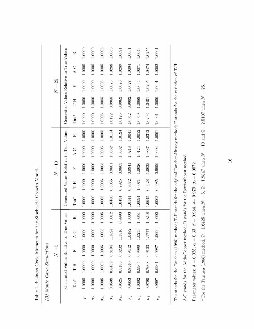
Table2BusinessCycleMomentsfortheStochasticGrowthModel:

(B)MonteCarloSimulations

N=5

N=10

N=25

GeneratedValuesRelativetoTrueValues

GeneratedValuesRelativetoTrueValues

GeneratedValuesRelativetoTrueValues

Tau*

T-H

FA-C

RTau*

T-H

FA-C

RTau*

T-H

FA-C

R

1.0000

1.0000

1.0000

1.0000

1.0000

1.0000

1.0000

1.0000

1.0000

1.0000

1.0000

1.0000

1.0000

1.0000

1.0000

"

1.0000

1.0000

1.0000

1.0000

1.0000

1.0000

1.0000

1.0000

1.0000

1.0000

1.0000

1.0000

1.0000

1.0000

1.0000

a

1.0005

1.0005

1.0005

1.0005

1.0005

1.0005

1.0005

1.0005

1.0005

1.0005

1.0005

1.0005

1.0005

1.0005

1.0005

k

0.9508

0.5439

0.8194

1.1524

1.0012

1.0450

0.8066

0.9801

1.0682

1.0114

1.0122

0.9968

1.0075

1.0288

1.0085

ka

0.9525

0.5185

0.8202

1.1516

0.9993

1.0434

0.7925

0.9803

1.0682

1.0124

1.0125

0.9962

1.0076

1.0289

1.0091

y

0.9853

0.8540

0.9442

1.0482

1.0003

1.0141

0.9372

0.9941

1.0218

1.0041

1.0042

0.9992

1.0027

1.0094

1.0031

c

1.0002

0.9965

0.9990

1.0253

1.0051

1.0094

1.0071

1.0026

1.0124

1.0052

1.0049

1.0089

1.0034

1.0071

1.0043

i

0.9790

0.7608

0.9103

1.1777

1.0248

1.0645

0.9428

1.0033

1.0887

1.0312

1.0293

1.0401

1.0205

1.0474

1.0255

y

0.9997

0.9961

0.9987

1.0009

1.0000

1.0003

0.9985

0.9999

1.0004

1.0001

1.0001

1.0000

1.0001

1.0002

1.0001

TaustandsfortheTauchen(1986)method;T-HstandsfortheoriginalTauchen-Husseymethod;FstandsforthevariationofT-H;

A-CstandsfortheAdda-Coopermethod;RstandsfortheRouwenhorstmethod.

Parametervalues:=0:025;=0:33;=0:984;=0:979;"=0:0072:

*FortheTauchen(1986)method,=1:6425whenN=5;=1:9847whenN=10and=2:5107whenN=25:

16

Table3MeasuresofInequalityfortheIncomeFluctuationProblem

(A)BaselineApproach

N=10

N=25

GeneratedValuesRelativetoTrueValues

GeneratedValuesRelativetoTrueValues

Aiyagari(1994)values:=0:9,=0:2

Tau*

T-H

FA-C

RTau*

T-H

FA-C

R

AR(1)process

0.9978

0.9976

0.9999

1.0087

1.0000

0.9996

1.0000

1.0000

1.0024

1.0000

1.0000

0.9462

0.9969

0.9793

1.0000

1.0000

0.9996

1.0000

0.9937

1.0000

LaborEndowment(et)

CV

0.9725

0.9187

0.9921

0.9402

0.9862

0.9890

0.9996

1.0010

0.9734

0.9954

Consumption(ct)

CV

0.9038

0.8631

0.8555

0.8500

0.9497

0.9435

0.9641

0.9659

0.9131

0.9598

Gini

0.9112

0.8709

0.9511

0.8621

0.9479

0.9433

0.9569

0.9579

0.9194

0.9541

TotalIncome(we t+rat)

CV

0.9162

0.8783

0.9496

0.8801

0.9430

0.9418

0.9571

0.9586

0.9211

0.9527

Gini

0.9554

0.9176

0.9707

0.9284

0.9701

0.9685

0.9746

0.9752

0.9560

0.9733

Assets(a

t)CV

0.6487

0.6571

0.6877

0.6271

0.6793

0.6759

0.6928

0.6939

0.6574

0.6884

Gini

0.7626

0.7707

0.7906

0.7453

0.7849

0.7829

0.7931

0.7934

0.7707

0.7902

French(2005)values:=0:977,=0:12

Tau*

T-H

FA-C

RTau*

T-H

FA-C

R

AR(1)process

0.9987

0.9872

1.0004

1.0040

1.0000

0.9997

0.9982

1.0000

1.0013

1.000

1.0000

0.6084

0.9587

0.9793

1.0000

1.000

0.8683

0.9996

0.9937

1.000

LaborEndowment(et)

CV

0.9365

0.5594

0.9111

0.9203

0.9794

0.9665

0.8131

0.9999

0.9622

0.9937

Consumption(ct)

CV

0.8352

0.4906

0.8878

0.7884

0.9331

0.9021

0.7581

0.9529

0.8807

0.9465

Gini

0.9079

0.5471

0.9392

0.8631

0.9694

0.9548

0.8264

0.9771

0.9410

0.9746

TotalIncome(we t+rat)

CV

0.8540

0.5363

0.8813

0.8229

0.9351

0.9101

0.7759

0.9556

0.8962

0.9490

Gini

0.9514

0.6185

0.9578

0.9216

0.9921

0.9831

0.8669

0.9988

0.9741

0.9967

Assets(a

t)CV

0.5026

0.5002

0.5851

0.4814

0.5885

0.5613

0.5337

0.6021

0.5486

0.5974

Gini

0.7229

0.7246

0.7986

0.7005

0.7904

0.7726

0.7566

0.7985

0.7651

0.7956

Notation:andarethepersistenceandthestandarddeviationoflne t.Parametervalues:=0:96;r=0:0375,w=1:

*UndertheAiyagari(1994)calibration,=2:2540whenN=10and=2:8176whenN=25:UndertheFrench(2005)

calibration,=1:9986whenN=10and=2:5307whenN=25:

17

Table3MeasuresofInequalityfortheIncomeFluctuationProblem

(B)MonteCarloSimulations

N=10

N=25

GeneratedValuesRelativetoTrueValues

GeneratedValuesRelativetoTrueValues

Aiyagari(1994)values:=0:9,=0:2

Tau*

T-H

FA-C

RTau*

T-H

FA-C

R

AR(1)process

0.9999

0.9999

0.9999

0.9999

0.9999

0.9999

0.9999

0.9999

0.9999

0.9999

0.9998

0.9998

0.9998

0.9998

0.9998

0.9998

0.9998

0.9998

0.9998

0.9998

LaborEndowment(et)

CV

0.9985

0.9985

0.9985

0.9985

0.9985

0.9985

0.9985

0.9985

0.9985

0.9985

Consumption(ct)

CV

0.9636

0.9682

0.9612

0.9625

0.9602

0.9634

0.9626

0.9623

0.9619

0.9621

Gini

0.9559

0.9605

0.9537

0.9551

0.9528

0.9554

0.9546

0.9543

0.9544

0.9541

TotalIncome(we t+rat)

CV

0.9554

0.9579

0.9526

0.9558

0.9513

0.9562

0.9554

0.9548

0.9556

0.9545

Gini

0.9740

0.9771

0.9711

0.9751

0.9701

0.9738

0.9730

0.9725

0.9737

0.9723

Assets(a

t)CV

0.6856

0.6925

0.6791

0.6906

0.6751

0.6917

0.6901

0.6875

0.6913

0.6864

Gini

0.7870

0.7954

0.7806

0.7941

0.7770

0.7912

0.7897

0.7874

0.7925

0.7864

French(2005)values:=0:977,=0:12

Tau*

T-H

FA-C

RTau*

T-H

FA-C

R

AR(1)process

0.9999

0.9999

0.9999

0.9999

0.9999

0.9999

0.9999

0.9999

0.9999

0.9999

0.9988

0.9988

0.9988

0.9988

0.9988

0.9988

0.9988

0.9988

0.9988

0.9988

LaborEndowment(et)

CV

0.9988

0.9988

0.9988

0.9988

0.9988

0.9988

0.9988

0.9988

0.9988

0.9988

Consumption(ct)

CV

0.9682

1.0355

0.9204

0.9812

0.9479

0.9632

0.9928

0.9520

0.9721

0.9511

Gini

0.9926

1.0683

0.9489

1.0076

0.9727

0.9838

1.0156

0.9751

0.9917

0.9745

TotalIncome(we t+rat)

CV

0.9675

1.0198

0.9231

0.9780

0.9501

0.9645

0.9887

0.9546

0.9722

0.9536

Gini

1.0139

1.0809

0.9727

1.0274

0.9949

1.0051

1.0342

0.9971

1.0119

0.9965

Assets(a

t)CV

0.5864

0.5981

0.5790

0.5862

0.5855

0.6050

0.6122

0.6007

0.6115

0.5969

Gini

0.7860

0.8117

0.7851

0.7899

0.7836

0.7984

0.8156

0.7965

0.8048

0.7932

Notation:andarethepersistenceandthestandarddeviationoflne t.Parametervalues:=0:96;r=0:0375,w=1:

*UndertheAiyagari(1994)calibration,=2:2540whenN=10and=2:8176whenN=25:UndertheFrench(2005)

calibration,=1:9986whenN=10and=2:5307whenN=25:

18

5 Appendix

Preliminaries

In this section we derive a set of equations that are useful in the following proofs. First using the binomial

formula, the elements in the first and the last rows of ΠN can be expressed as

π(N)1,j =

(N − 1j − 1

)pN−j (1− p)j−1 , (10)

and

π(N)N,j =

(N − 1j − 1

)(1− q)N−j qj−1, (11)

for j = 1, 2, ..., N. For all other rows, the elements in ΠN can be defined recursively using the elements

in ΠN−1. Begin with the system for N − 1 ≥ 2. The system of polynomials is given by

Φ (t;N − 1, i) = [p + (1− p) t]N−1−i (1− q + qt)i−1 =N−1∑

j=1

π(N−1)i,j tj−1,

for i = 1, ..., N − 1. There are two ways to relate this system to the one for N :

Φ (t; N, i) = [p + (1− p) t] Φ (t;N − 1, i) , (12)

for i = 1, ..., N − 1, and

Φ (t;N, i) = (1− q + qt)Φ (t; N − 1, i− 1) , (13)

for i = 2, ..., N. Substituting (3) into (12) and rearranging terms gives

N∑

j=1

π(N)i,j tj−1 =

N−1∑

j=1

pπ(N−1)i,j tj−1 +

N−1∑

j=1

(1− p)π(N−1)i,j tj ,

for i = 1, ..., N − 1. Similarly, substituting (3) into (13) would give

N∑

j=1

π(N)i,j tj−1 =

N−1∑

j=1

(1− q) π(N−1)(i−1),jt

j−1 +N−1∑

j=1

qπ(N−1)(i−1),jt

j ,

for i = 2, ..., N. The following can be obtained by comparing the coefficients for i = 1, 2, ..., N − 1,

π(N)i,1 = pπ

(N−1)i,1 = (1− q) π

(N−1)(i−1),1, (14)

19

π(N)i,j = pπ

(N−1)i,j + (1− p) π

(N−1)i,(j−1) = (1− q) π

(N)(i−1),j + qπ

(N)(i−1),(j−1), (15)

for j = 2, ..., N − 1, and

π(N)i,N = (1− p) π

(N−1)i,(N−1) = qπ

(N−1)(i−1),N . (16)

Proof of Proposition 1

For any N ≥ 2, the elements in the Rouwenhorst matrix ΘN =[θ(N)i,j

]are governed by the following

equations: For the elements in the first row,

θ(N)1,j =

pθ(N−1)1,j , if j = 1,

pθ(N−1)1,j + (1− p) θ

(N−1)1,(j−1), if j = 2, ..., N − 1,

(1− p) θ(N−1)1,(j−1), if j = N.

(17)

For the elements in the final row,

θ(N)N,j =

(1− q) θ(N−1)(N−1),j , if j = 1,

(1− q) θ(N−1)(N−1),j + qθ

(N−1)(N−1),(j−1), if j = 2, ..., N − 1,

qθ(N−1)(N−1),(j−1), if j = N.

(18)

For the elements in row i = 2, ..., N − 1,

θ(N)i,j =

12

[pθ

(N−1)i,j + (1− q) θ

(N−1)(i−1),j

], if j = 1,

12

[(1− p) θ

(N−1)i,(j−1) + qθ

(N−1)(i−1),(j−1)

], if j = N,

(19)

and for j = 2, ..., N − 1,

θ(N)i,j =

12

[pθ

(N−1)i,j + (1− p) θ

(N−1)i,(j−1) + (1− q) θ

(N−1)(i−1),j + qθ

(N−1)(i−1),(j−1)

], (20)

For any given ΘN−1, the system of equations (17)-(20) defines a unique ΘN . Similarly, for any given

ΠN−1, the system of equations (10)-(16) defines a unique ΠN . Since Θ2 = Π2, it suffices to show that

the system (10)-(16) coincides with the system (17)-(20).

Consider the first row (i.e., i = 1) in ΠN . According to (10), π(N)1,1 = pπ

(N−1)1,1 , and π

(N)1,N = (1− p) π

(N−1)1,(N−1).

For j = 2, ..., N − 1, since

π(N−1)1,j =

(N − 2j − 1

)pN−1−j (1− p)j−1 ,

20

and (N − 1j − 1

)=

(N − 2j − 1

)+

(N − 2j − 2

),

we have

π(N)1,j = pπ

(N−1)1,j + (1− p) π

(N−1)1,(j−1).

This shows that the elements in the first row of ΠN satisfy (17). Using (11) and the same procedure, one

can show that the elements in the last row of ΠN satisfy (18). The rest of the proof follows immediately

from (14)-(16). For instance, for any row i = 2, ..., N − 1 in ΠN , (14) implies

π(N)i,1 =

12

[pπ

(N−1)i,1 + (1− q) π

(N−1)(i−1),1

].

This coincides with the first equation in (19). Similarly, (15) and (16) can be used to derive the remaining

equations in (19) and (20). Thus all the elements in row i = 2, ..., N − 1 in ΠN satisfies (19) and (20).

This completes the proof.

Proof of Proposition 3

As mentioned in the proof of Proposition 1, the first column of ΠN is given by

π(N)i,1 = pN−i (1− q)i−1 ,

for i = 1, 2, ..., N. Define λ(N)

i as in (4). Then

N∑

i=1

λ(N)

i π(N)i,1 = [sp + (1− s) (1− q)]N = sN = λ

(N)

1 .

For all other columns except the first one, an induction argument is used. First we know that the guess

is correct when N = 2. Suppose the guess is correct for some N ≥ 2, i.e.,

λ(N)

j =N∑

i=1

λ(N)

i π(N)i,j , for j = 1, 2, ..., N. (21)

21

We have already proved that this is true when j = 1, so proceed to j = 2, ..., N + 1. Using (4), the

following can be derived

λ(N+1)

i =

sλ(N)

i , for i = 1,

sλ(N)

i + (1− s) λ(N)

i−1 , for i = 2, ..., N,

(1− s) λ(N)

i−1 , for i = N + 1.

(22)

Using these one can obtain

N+1∑

i=1

λ(N+1)

i π(N+1)i,j =

N∑

i=1

sλ(N)

i π(N+1)i,j +

N∑

i=1

(1− s) λ(N)

i π(N+1)(i+1),j . (23)

A more detailed derivation of this result can be found in Kopecky and Suen (2009). Based on (15), the

following can be obtained

π(N+1)i,j = pπ

(N)i,j + (1− p) π

(N)i,j−1,

and

π(N+1)i+1,j = (1− q) π

(N)i,j + qπ

(N)i,(j−1),

for j = 2, 3, ..., N. Substituting these into (23) and rearranging terms gives

N+1∑

i=1

λ(N+1)

i π(N+1)i,j

= [sp + (1− s) (1− q)]N∑

i=1

λ(N)

i π(N)i,j + [s (1− p) + (1− s) q]

N∑

i=1

λ(N)

i π(N)i,(j−1).

Using the induction hypothesis (21) and (22) gives,

N+1∑

i=1

λ(N+1)

i π(N+1)i,j = sλ

(N)

j + (1− s) λ(N)

j−1 = λ(N+1)

j ,

for j = 2, 3, ..., N. Since∑N+1

i=1 λ(N+1)

i = 1 and∑N+1

j=1 π(N+1)i,j = 1, the remaining equation for j = N + 1

must be satisfied. This completes the proof.

22

References

[1] Adda, J., Cooper, R., 2003. Dynamic Economics: Quantitative Methods and Applications. MIT

Press, Cambridge, MA.

[2] Aiyagari, S.R., 1994. Uninsured Idiosyncratic Risk and Aggregate Saving. Quarterly Journal of

Economics 109, 659-684.

[3] Aruoba, S., Fernandez-Villaverde, J., Rubio-Ramırez, J., 2006. Comparing Solution Methods for

Dynamic Equilibrium Economies. Journal of Economic Dynamics and Control 30, 2477-2508.

[4] Burnside, C., 1999. Discrete State-Space Methods for the Study of Dynamic Economies. In: Ma-

rimon, R., Scott, A. (Ed.), Computational Methods for the Study of Dynamic Economies. Oxford

University Press, Oxford, 95-113.

[5] Chang, Y., Kim, S., 2006. From Individual to Aggregate Labor Supply: A Quantitative Analysis

Based on a Heterogeneous Agent Economy. International Economic Review 47, 1-27.

[6] Chang, Y., Kim, S., 2007. Heterogeneity and Aggregation: Implications for Labor-Market Fluctu-

ations. American Economic Review 97, 1939-1956.

[7] Christiano, L., Fisher, J., 2000. Algorithms for Solving Dynamic Models with Occasionally Binding

Constraints. Journal of Economic Dynamics and Control 24, 1179-1232.

[8] den Haan, W.J., 2010. Comparison of Solutions to the Incomplete Markets Model with Aggregate

Uncertainty. Journal of Economic Dynamics and Control 34, 4-27.

[9] Floden, M., 2008a. A Note on the Accuracy of Markov-chain Approximations to Highly Persistent

AR(1) Processes. Economics Letters 99, 516-520.

[10] Floden, M., 2008b. Aggregate Savings When Individual Income Varies. Review of Economic Dy-

namics 11, 70-82.

[11] French, E., 2005. The Effects of Health, Wealth, and Wages on Labor Supply and Retirement

Behaviour. Review of Economic Studies 72, 395-427.

[12] King, R.G., Rebelo, S.T., 1999. Resuscitating Real Business Cycles. In: Taylor, B.J., Woodford, M.

(Ed.), Handbook of Macroeconomics, Volume 1. Elsevier, Amsterdam, 927-1007.

23

[13] Kopecky, K.A., Suen, R., 2009. Finite State Markov-chain Approximations to Highly Persistent

Processes. Working paper version.

[14] Krusell, P., Mukoyama, T., Sahin, A., Smith, A.A., 2009. Revisiting the Welfare Effects of Elimi-

nating Business Cycles. Review of Economic Dynamics 12, 393-404.

[15] Krusell, P., Smith, A.A., 1998. Income and Wealth Heterogeneity in the Macroeconomy. Journal of

Political Economy 106, 867-896.

[16] Lkhagvasuren, D., Galindev, R., 2008. Discretization of Highly-Persistent Correlated AR(1) Shocks.

Unpublished manuscript, Concordia University.

[17] Pijoan-Mas, J., 2006. Precautionary Savings or Working Longer Hours? Review of Economic Dy-

namics 9, 326-352.

[18] Rouwenhorst, K.G., 1995. Asset Pricing Implications of Equilibrium Business Cycle Models. In:

Cooley, T.F. (Ed.), Frontiers of Business Cycle Research. Princeton University Press, Princeton,

NJ, 294-330.

[19] Santos, M.S., Peralta-Alva, A., 2005. Accuracy of Simulations for Stochastic Dynamic Models.

Econometrica 73, 1939-1976.

[20] Storesletten, K., Telmer, C., Yaron, A., 1999. The Risk-Sharing Implications of Alternative Social

Security Arrangements. Carnegie-Rochester Conference Series on Public Policy 50, 213-259.

[21] Tauchen, G., 1986. Finite State Markov-chain Approximations to Univariate and Vector Autore-

gressions. Economics Letters 20, 177-181.

[22] Tauchen, G., 1990. Solving the Stochastic Growth Model by using Quadrature Methods and Value-

Function Iterations. Journal of Business and Economic Statistics 8, 49-51.

[23] Tauchen, G., Hussey, R., 1991. Quadrature-Based Methods for Obtaining Approximate Solutions

to Nonlinear Asset Pricing Models. Econometrica 59, 371-396.

[24] Taylor, J., Uhlig, H., 1990. Solving Nonlinear Stochastic Growth Models: A Comparison of Alter-

native Solution Methods. Journal of Business and Economic Statistics 8, 1-18.

24