Finite rate chemistry effects and combustor liner heat transfer studies in a framework of LES of turbulent flames

- investigation of pollutant formation using OpenFOAM

Dr. Karl-Johan NogenmyrProf. C.K. Chan

Dept. Applied Mathematics, The Hong Kong Polytechnic University

Dr. Christophe DuwigDept. of Energy Sciences, Lund University, Sweden

Fifth OpenFOAM WorkshopJune 21-24 2010

Gothenburg, Sweden

Outline of presentation

• reactingLMFoam – the low Mach number LES combustion code– Code description– Typical setup

• Case A: A high speed jet flame, Sydney PPJB– Setup and flame shape– Computed case, preliminary results

• Case B: A lean premixed swirling turbulent flame– Burner specification– Computed cases, preliminary results

• Conclusions

reactingLMFoam

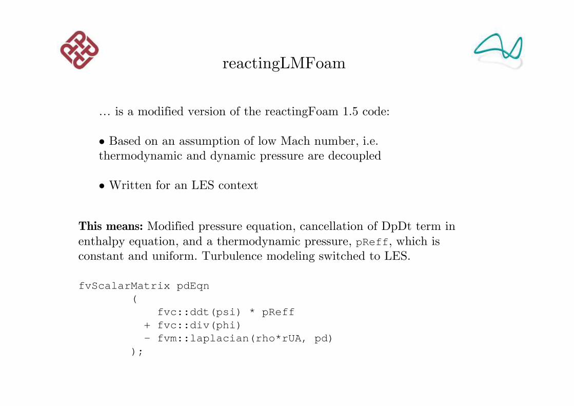
… is a modified version of the reactingFoam 1.5 code:

• Based on an assumption of low Mach number, i.e. thermodynamic and dynamic pressure are decoupled

• Written for an LES context

This means: Modified pressure equation, cancellation of DpDt term in enthalpy equation, and a thermodynamic pressure, pReff, which is constant and uniform. Turbulence modeling switched to LES.

fvScalarMatrix pdEqn(

fvc::ddt(psi) * pReff+ fvc::div(phi)- fvm::laplacian(rho*rUA, pd)

);

�

T

( ) ( ) 0 ,

( ) ( ) ( 2 3tr ( ) ) ,

( ) ( ) ( Sc ) ( , ) ,

( ) ( ) ( Pr ) ,

t

t t

t i i t i j i

t t

p

Y Y Y w Y T

h h T

∂ ρ ρ∂ ρ ρ µ ρ∂ ρ ρ µ κ∂ ρ ρ µ

⊗

+∇⋅ = +∇⋅ = ∇⋅ ∇ +∇ − ∇ −∇ + +∇⋅ = ∇⋅ ∇ + +∇⋅ = ∇⋅ ∇

v

v v v v v v I g

v

v

ɶ

ɶ ɶ ɶ ɶ ɶ ɶ

ɶ ɶ ɶ ɶ ɶɶ ɺ

ɶ ɶɶ

t kc kµ µ ρ= + ∆

reactingLMFoam

Solved equations, the Favre filtered Navier-Stokes with species and enthalpy transport:

0p

RTρ =

Since a low Mach number approach is used, p0 is a uniform constantUnity Schmidt and Prandtl numbers are assumed.

With Smagorinsky to express subgrid turbulence kinetic energy, k, the equations are closed:

Equation of state to determine density:

reactingLMFoam - Suitable operating conditions:

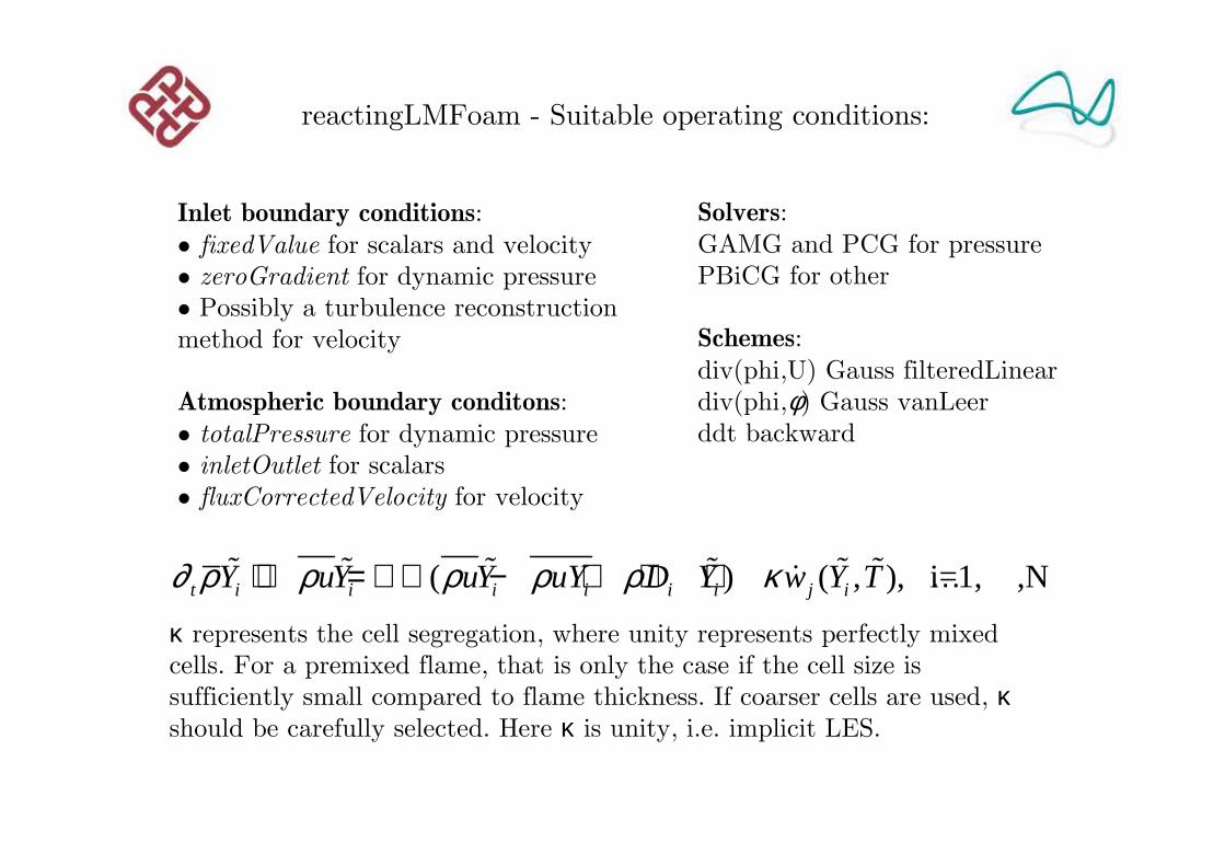
Inlet boundary conditions:• fixedValue for scalars and velocity• zeroGradient for dynamic pressure• Possibly a turbulence reconstruction method for velocity

Atmospheric boundary conditons:• totalPressure for dynamic pressure• inletOutlet for scalars• fluxCorrectedVelocity for velocity

Solvers:GAMG and PCG for pressurePBiCG for other

Schemes:div(phi,U) Gauss filteredLineardiv(phi,φ) Gauss vanLeerddt backward

( ) ( , ), i=1, ,Nt i i i i i i j iY uY uY uY D Y w Y T∂ ρ ρ ρ ρ ρ κ+ ∇ = ∇ ⋅ − + ∇ + …ɶ ɶ ɶ ɶ ɶ ɶɺ

κ represents the cell segregation, where unity represents perfectly mixed cells. For a premixed flame, that is only the case if the cell size is sufficiently small compared to flame thickness. If coarser cells are used, κshould be carefully selected. Here κ is unity, i.e. implicit LES.

Case A – The well documented Sydney piloted premixed jet flame

Dunn et al. Combust&Flame 151

pp. 46-60

Case A – The well documented Sydney piloted premixed jet flame (B)

PILOT

PILOT

JET

PILOT

PILOT

JET

T

OH

A high speed lean methane jet (φ=0.5, U=100 m/s) surrounded by a pilot (φ=1.0, U=0.7 m/s)

Dunn et al. Combust&Flame 151 pp. 46-60

Experimental data kindly provided by Matthew Dunn, Sandia

Computed conditions and setup

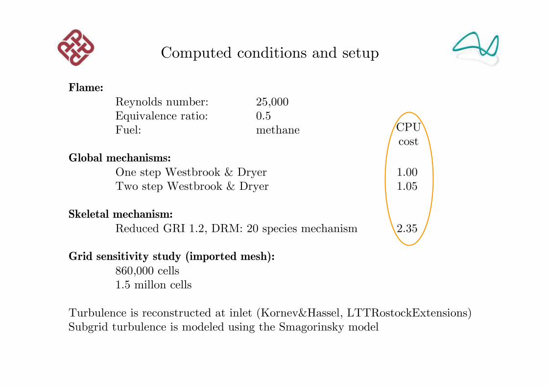
Flame:Reynolds number: 25,000Equivalence ratio: 0.5Fuel: methane

Global mechanisms:One step Westbrook & Dryer 1.00Two step Westbrook & Dryer 1.05

Skeletal mechanism:Reduced GRI 1.2, DRM: 20 species mechanism 2.35

Grid sensitivity study (imported mesh):860,000 cells1.5 millon cells

Turbulence is reconstructed at inlet (Kornev&Hassel, LTTRostockExtensions)Subgrid turbulence is modeled using the Smagorinsky model

CPUcost

Temperature and OH fields

As the jet is turbulent already at the inlet, unsteady structures develop immediately at the entrance. Strong mixing in the reacting layer shows the effects of the finite reaction rate.

860,000 cells20 speciesImplicit LES

Conclusions – Case A

• Promising results, even using a relatively simple model

• If cells are distributed to keep good resolution where reaction is intense, grid independent solutions is found already at ~ 1 million cells

• Profiles of intermediate species are captured when using skeletal mechanism. Though with a cost increase by a factor of ~ 2.3

• Effects of the finite reaction rate is captured

Case B - the Hong Kong swirl burner

• Axial feed from centre pipe (d=16 mm)

• Swirl feed from the two small pipes

• Swirl injected in four channels

Swirl number: zero to 1.7Reynolds number: no restrictionEquivalence ratio: no restriction

Open Confined

In a case study, the influence of a typical gas turbine combustor is assessed.

Velocity field prediction is verified with PIV data.

Influence of wall temperature on the flame is analyzed.

(mm)

Computed conditions and setup

Reynolds number: 10,000Swirl number: 0.8Equivalence ratio: 0.9 and 0Fuel: methane

For reacting cases, reactingLMFoam is usedFor non-reacting cases, oodles is used

Steady inflow, located far upstreamTurbulence is modelled using the Smagorinsky model

Two-step Westbrook & Dryer methane mechanism is used:CH4 + 1.5O2 => CO + 2H2O CO2 <=> CO + 0.5O2

( ) 2ax ax tang

D DSw

2 8 ( 1)

L w

D p wh m m

π −= =+

ɺ

ɺ ɺ ɺ

Two meshes are generated using snappyHexMesh.STL:s from proprietary 3D modeling software.

The capabilities of snappy the mesh complex geometries are appreciated.

1 million cells 1.3 million cells

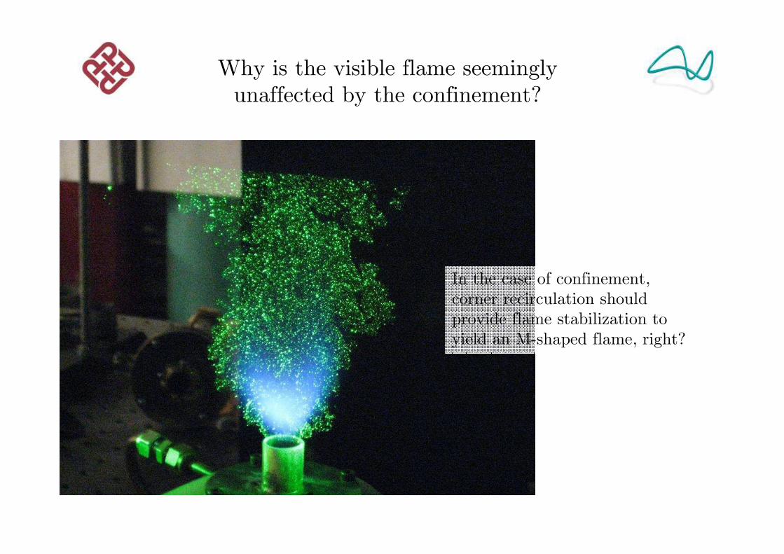
Why is the visible flame seemingly unaffected by the confinement?

In the case of confinement, corner recirculation should provide flame stabilization to yield an M-shaped flame, right?

Influence of wall temperature- on temperature field

Adiabatic ‘Realistic’

A separate simulation, using a skeletal mechanism with 20 species, and a separate mesh with an y+ about 2

Tw~800K

Tw~1040K

Tw~800K

Corner fluid approaches wall T

Adiabatic ‘Realistic’

Influence of wall temperature- on flame shape

A separate simulation, using a skeletal mechanism with 20 species, and a separate mesh with an y+ about 2

Lack of corner stabilization

Conclusions – Case B

• Simulation results look encouraging – physics is captured

• snappyHexMesh is applied successfully

• The finite rate chemistry code can handle different combustion situations, premixed and stratified premixed.

• Effects of heat transfer on flame shape is illustrated and solver gives realistic results.

Thank you for your attention!