Embed Size (px)
Citation preview

Finite Elements”from the early beginning to the very end”
x
A(x), E(x)
hb(x)g
x = Lx = 0.
An Introduction to
Elasticity and Heat Transfer
Applications
Preliminary edition
LiU-IEI-S--08/535--SE
Bo Torstenfelt


Contents
1 Prelude 11.1 Background . . . . . . . . . . . . . . . . . . . . . . . . . . . . . . . 21.2 The Big Picture . . . . . . . . . . . . . . . . . . . . . . . . . . . . . 3
I Linear Static Elasticity 5
2 Introduction 7
3 Bars 93.1 The Bar Displacement Assumption . . . . . . . . . . . . . . . . . . 93.2 The Local Equations . . . . . . . . . . . . . . . . . . . . . . . . . . 103.3 A Strong Formulation . . . . . . . . . . . . . . . . . . . . . . . . . 123.4 A Weak Formulation . . . . . . . . . . . . . . . . . . . . . . . . . . 133.5 A Galerkin Formulation . . . . . . . . . . . . . . . . . . . . . . . . 143.6 A Matrix Formulation . . . . . . . . . . . . . . . . . . . . . . . . . 203.7 A 2-Node Element Stiffness Matrix . . . . . . . . . . . . . . . . . . 213.8 A 3-Node Element Stiffness Matrix . . . . . . . . . . . . . . . . . . 253.9 An Element Load Vector . . . . . . . . . . . . . . . . . . . . . . . . 263.10 The Assembly Operation . . . . . . . . . . . . . . . . . . . . . . . . 283.11 Stress and Strain Calculations . . . . . . . . . . . . . . . . . . . . . 283.12 Multi-dimensional Truss Frame Works . . . . . . . . . . . . . . . . 293.13 Numerical Examples . . . . . . . . . . . . . . . . . . . . . . . . . . 32
A 1D bar problem . . . . . . . . . . . . . . . . . . . . . . . . . . . 32A 2D truss problem . . . . . . . . . . . . . . . . . . . . . . . . . . 36A 3D truss problem . . . . . . . . . . . . . . . . . . . . . . . . . . 39
3.14 Common Pitfalls and Mistakes . . . . . . . . . . . . . . . . . . . . 403.15 Summary . . . . . . . . . . . . . . . . . . . . . . . . . . . . . . . . 42
i

ii CONTENTS
4 Beams 454.1 The Beam Displacement Assumption . . . . . . . . . . . . . . . . . 464.2 The Local Equations . . . . . . . . . . . . . . . . . . . . . . . . . . 464.3 A Strong Formulation . . . . . . . . . . . . . . . . . . . . . . . . . 494.4 A Weak Formulation . . . . . . . . . . . . . . . . . . . . . . . . . . 504.5 A Galerkin Formulation . . . . . . . . . . . . . . . . . . . . . . . . 524.6 A Matrix Formulation . . . . . . . . . . . . . . . . . . . . . . . . . 544.7 A 2D 2-node Beam Element . . . . . . . . . . . . . . . . . . . . . . 554.8 An Element Load Vector . . . . . . . . . . . . . . . . . . . . . . . . 594.9 A 2D Beam Element with Axial Stiffness . . . . . . . . . . . . . . . 614.10 A 3D Space Frame Element . . . . . . . . . . . . . . . . . . . . . . 624.11 Stress and Strain Calculations . . . . . . . . . . . . . . . . . . . . . 644.12 Numerical Examples . . . . . . . . . . . . . . . . . . . . . . . . . . 66
A 2D console beam . . . . . . . . . . . . . . . . . . . . . . . . . . . 664.13 Summary . . . . . . . . . . . . . . . . . . . . . . . . . . . . . . . . 69
5 Solids 735.1 Displacement Assumptions . . . . . . . . . . . . . . . . . . . . . . 74
The 2D Membrane Displacement Assumption . . . . . . . . . . . . 74The Axisymmetric Displacement Assumption . . . . . . . . . . . . 75The 3D Displacement Assumption . . . . . . . . . . . . . . . . . . 77
5.2 Unknown Stress Components . . . . . . . . . . . . . . . . . . . . . 775.3 The Local Equations . . . . . . . . . . . . . . . . . . . . . . . . . . 80
The Balance law . . . . . . . . . . . . . . . . . . . . . . . . . . . . 80The Constitutive relation . . . . . . . . . . . . . . . . . . . . . . . 81The Compatibility relation . . . . . . . . . . . . . . . . . . . . . . 83A Summary of Local Equations . . . . . . . . . . . . . . . . . . . . 84
5.4 A Strong Formulation . . . . . . . . . . . . . . . . . . . . . . . . . 855.5 A Weak Formulation . . . . . . . . . . . . . . . . . . . . . . . . . . 865.6 The Galerkin Formulation . . . . . . . . . . . . . . . . . . . . . . . 905.7 The Matrix Problem . . . . . . . . . . . . . . . . . . . . . . . . . . 945.8 The Assembly Operation . . . . . . . . . . . . . . . . . . . . . . . . 965.9 The Element Load vector . . . . . . . . . . . . . . . . . . . . . . . 995.10 The 2D Constant Strain Triangle . . . . . . . . . . . . . . . . . . . 100
The Element Stiffness matrix . . . . . . . . . . . . . . . . . . . . . 100A Numerical Example . . . . . . . . . . . . . . . . . . . . . . . . . 106
5.11 Four-node Rectangular Aligned Elements . . . . . . . . . . . . . . 111A Numerical Example . . . . . . . . . . . . . . . . . . . . . . . . . 112
5.12 Isoparametric 2D Elements . . . . . . . . . . . . . . . . . . . . . . 115A 2D 4-node Quadrilateral Element . . . . . . . . . . . . . . . . . 115A Numerical Example . . . . . . . . . . . . . . . . . . . . . . . . . 120Numerical Integration . . . . . . . . . . . . . . . . . . . . . . . . . 125The Numerical Work Flow . . . . . . . . . . . . . . . . . . . . . . . 1292D 8- and 9-node Quadrilateral Elements . . . . . . . . . . . . . . 131

CONTENTS iii
Sub- or Hyperparametric Element Formulations . . . . . . . . . . . 1345.13 Isoparametric 3D Elements . . . . . . . . . . . . . . . . . . . . . . 1355.14 Isoparametric Axisymmetric Elements . . . . . . . . . . . . . . . . 1375.15 Distributed Loads . . . . . . . . . . . . . . . . . . . . . . . . . . . 139
Line Loads . . . . . . . . . . . . . . . . . . . . . . . . . . . . . . . 139Surface Loads . . . . . . . . . . . . . . . . . . . . . . . . . . . . . . 142Volume Loads . . . . . . . . . . . . . . . . . . . . . . . . . . . . . . 143
5.16 Reaction Forces . . . . . . . . . . . . . . . . . . . . . . . . . . . . . 1435.17 Stress Evaluation . . . . . . . . . . . . . . . . . . . . . . . . . . . . 1455.18 An Element Library . . . . . . . . . . . . . . . . . . . . . . . . . . 148
2D and Axisymmetric elements . . . . . . . . . . . . . . . . . . . . 1483D elements . . . . . . . . . . . . . . . . . . . . . . . . . . . . . . . 149
5.19 Summary . . . . . . . . . . . . . . . . . . . . . . . . . . . . . . . . 150
II Linear Heat Transfer 153
6 1D Steady-state Heat Transfer 1556.1 The Local Equations . . . . . . . . . . . . . . . . . . . . . . . . . . 1566.2 A Strong Formulation . . . . . . . . . . . . . . . . . . . . . . . . . 1576.3 A Weak Formulation . . . . . . . . . . . . . . . . . . . . . . . . . . 1586.4 A Galerkin Formulation . . . . . . . . . . . . . . . . . . . . . . . . 1596.5 A Matrix Formulation . . . . . . . . . . . . . . . . . . . . . . . . . 161
7 Multi-dim Transient Heat Transfer 1637.1 Local Equations . . . . . . . . . . . . . . . . . . . . . . . . . . . . 164
The Balance Law . . . . . . . . . . . . . . . . . . . . . . . . . . . . 165Constitutive Relation . . . . . . . . . . . . . . . . . . . . . . . . . . 167
7.2 Strong Formulation . . . . . . . . . . . . . . . . . . . . . . . . . . . 1687.3 Weak Formulation . . . . . . . . . . . . . . . . . . . . . . . . . . . 1697.4 Galerkin Formulation . . . . . . . . . . . . . . . . . . . . . . . . . . 1707.5 Matrix Formulation . . . . . . . . . . . . . . . . . . . . . . . . . . 172

iv CONTENTS

Preface
The writing of this book has arisen as a natural next step in my profession as ateacher, researcher, program developer, and user of the Finite Element Method.Of course one can wonder, why I am writing just another book in Finite Elements.The answer is equally obvious as simple. After many years in the field I have, ashave many others, discovered a large variety of pitfalls or mistake done by othersand myself. I have now reached a point where I would like to describe my viewof the topic. That is, how to understand it, how to teach it, how to implement itand how to use it; these will be main goals for the discussion to come!
The discussion to come will be influenced by experiences from all four of thesebranches. As a teacher I have taught both basic and advanced courses in FiniteElements with focus on both Solid Mechanics and Heat Transfer applications.These courses have been given at the Linkoping University in the mechanicalengineering programme.
The text to come is written by an engineer for engineers. One overall goalfor the description is to try to cover every step from how a certain mathematicalmodel appears from basic considerations based on fact from reality, to a classicalformulation with its possible analytical solutions, and finally over to a study ofnumerical solutions used by a Finite Element program based on a certain finiteelement formulation.
That is, discussing the finite element method from the early beginning to thevery end.
The great challenge is to make this as short and interesting as possible withoutloosing or breaking the mathematical chain. It is strongly believed that forsuccess in learning Finite Elements it is an absolute prerequisite to be familiarwith the local equations and their available analytical solutions. I think mostpeople who have tried to teach Finite Elements agree upon this, traditionallyhowever, most education in Finite Elements is given in separate courses. Whynot try to teach Finite Elements in close connection to where the basic materialis taught. That is, integrate Finite Elements together with basic material in the
v

same course!Of course, Finite Elements can be taught as a weighted residual method for
approximate solutions of sets of coupled partial differential equations withoutdiscussing any physical application and just focusing on existence, uniquenessand error bounds of the solution. This is of course also important but for moststudents studying different engineering disciplines Finite Elements will be a toolfor trying to understand and predict the behavior of reality. An important focusin studies of finite element formulations of different engineering disciplines is tobe aware what should be expected of the quality of the approximate numericalsolution. This can only be learnt by knowing the most important details ofthe mathematical background and then solving numerical problems having ananalytical solution to compare with.
Another aspect important for engineers working with the method as a dailytool, is how to use the method as efficiently as possible both from a time-consuming and a computer resources point of view.
Over a period of at least 15 years I have worked with the graphical finiteelement environment TRINITAS. This is a stand-alone tool for optimization,conceptual design and education as well as for general linear elasticity and heattransfer problem both as steady-state, transient or as eigenvalue problems. It isan Object Oriented program based on a graphical user interface for manipulationof the database of the program. This program contains procedures for geometrymodeling, domain property and boundary conditions definition, mesh generation,finite element analysis and result evaluation. The program is used in eduction atdifferent levels. It is used in basic courses in Finite Elements at an undergraduatelevel and also in advanced course where the students add their own routines forinstance; element stiffness matrix, stress calculations in elasticity problems orutilizing ready-to-use routines for crack propagation analysis. This finite elementenvironment has also been used for testing of different research ideas and forsolving of different industrial engineering applications.
This program will be used throughout the text in this book as a tool foranalysis of all examples given during the discussion of different finite elementapplications.
The ideas and the arguments given above have been the main driving force fordoing this work. Hopefully, this book will prove useful as both an introductionof the method and also a standard tool or companion to be used during dailyfinite element work.
Bo Torstenfelt
November, 2007

Reader’s Instruction
Readers that have never studied Finite Elements are recommended to first readthe bar chapter (chap. 3) ”from the early beginning to the very end” very care-fully. It is the author’s belief that this chapter is detailed enough to serve asa stand-alone base for self-studies where the reader is recommended to, duringreading the text, perform a complete rewriting of the basic mathematical chain.
Every chapter to come is written in a manner and with an aim to be moreor less self-contained for the reader with sufficient pre-qualifications. Typicalrequired qualifications are 2 years studies at undergraduate level of any of themost common engineering programmes.
Concerning the layout of the text; there are important keywords which willappear as Margin text . As a student reading the text for the first time one should, Margin textafter reading a certain chapter or section, go back and use these margin textsas reminders for having reached a sufficient level of understanding of differentimportant concepts.
One major challenge when trying to describe Finite Elements is to give suffi-cient detail without making it too lengthy. That is the reason why some in-depthmaterial is given at the end of the book rather than where it appears for the firsttime.
vii


Notation
Notation principles used in this book are summarized below. If a letter or symbolis used twice with a different meaning, the letter or symbol will be given twicein this list.
As such, if a concept defined by a letter or symbol has several different usednames describing the same and equivalent interpretation, all will be given below.
General mathematical symbols
a A scalar valuea A column vector written as a bold lower-case letterai A coefficient in a vectorA A matrix written as a bold upper-case letterC0 The set of all continuous functionsC1 The set of all functions having a continuous first-order derivativeL Local equationsS Strong formulationW Weak formulationG Galerkin formulationM Matrix problemnsd Number of spatial dimensionsnel Number of elements belonging to the meshnn Number of nodes belonging to the meshne
n Number of nodes belonging to an elementnf Number of unknown freedoms in the meshnp Number of prescribed freedoms in the mesh
ix

Latin symbols
A An area or cross-sectional areaa The global unknown vector, the global displacement vector, the
global degrees of freedom (d.o.f.) vectorae An element-local unknown vector, element-local degrees of free-
dom (d.o.f.) vectorb, b Load per unit volume or lengthB Global kinematic matrixBe Element-local kinematic matrixCe Boolean connectivity matrixc, ci An arbitrary vector used for the weight functionc Element nodal coordinate vectorcp Specific heat coefficientxi, yi, zi Nodal coordinate componentsD Elasticity matrix in flexibility formD Thermal conductivity matrixE Young’s modulus of elasticityE Elasticity matrix in stiffness formf Global load vectorfd Global load vector from internal distributed forcesfg Global load vector from essential boundary conditionsfh Global load vector from natural boundary conditionsfr Global reaction force vectorG Shear modulusG Global operator matrix, gradient matrixg, g Essential boundary conditions (multi-dim or 1D)h, h Natural boundary conditions (multi-dim or 1D)I Area moment of inertiaJ Jacobian matrixK Global stiffness or conductivity matrixKe Element stiffness or conductivity matrixL LengthM Bending momentN Global shape function matrix

Ni A global shape functionN e Element-local shape function matrixNe
i A element-local shape functionN Axial force in bars or beamsQ Heat generation per unit lengthq, q Heat flux per unit surface (multi-dim or 1D)qn Heat flux perpendicular to the surfaceq Load per unit lengthR Residual vectorr Unbalanced force vector or discrete residual vectorT TemperatureT∞ Surrounding temperatureT Shear forcet Timet Thicknesst Traction vectorti A test functionS SurfaceS Statical moment, the first momentS Stress tensorSg The part of the surface where essential boundary conditions are
knownSh The part of the surface where natural boundary conditions are
knowns Stress vectoru Displacement vectoru, v, w Displacement vector componentsw, w Weight function (vector-valued or scalar-valued)V Volumex, y, z Global coordinates
Greek symbols
α Thermal expansion coefficientα Thermal convection coefficientδij Kronecker delta

φi A weight functionε Normal strainε Strain component vectorθi Nodal rotation componentλ Heat conductivityν Poisson’s ratio% Densityσij Normal stress componentτij Shear stress componentξ, η, ζ Local coordinates

Chapter 1Prelude
Nowadays Finite Elements are the standard tools for doing simulations in a largevariety of engineering disciplines. Finite Elements are no more a tool for just alimited number of enthusiastic experts; they are something all of us as engineershave to learn.
One reason for why this method still, to some extent, is looked upon as atechnique which you as an engineer can decide not to learn is probably becauseit is believed to be too difficult and time-consuming.
It is now time to change this option once for all. All of us can learn FiniteElements. Every engineer must know at least some basic facts from Finite Ele-ments applied to some of the most important fields of application. When tryingto learn Finite elements it is important and useful to have a solid knowledge ofthe physical problem, models of it and their analytical solutions. That is whyFinite Elements should be studied in close connection to overall basic studies ofa certain engineering discipline. Finite Elements is just a approximate numericaltool for solving some basic local equations constituting a mathematical model ofreality.
A reason for why this technique is still looked upon as difficult to learn isprobably that most text books are written by dedicated researcher in differentfields of finite element applications. As an author one probably tends to describethe method from a mathematical point of view as consistently as possible andwith a notation perhaps never previously seen by the students.
The technique is now so well-established that from a mathematical point ofview most features and deficiencies are known in a variety different mathematicalformulations of different important problems.
In this text we will learn why the method works, how the method works bothanalytically and numerically, how to use the method in typical daily engineeringapplications and, probably most important lesson what properties one should
1

2 1.1. BACKGROUND
expect form the numerical approximation of the unknown entities. It is theauthor’s intention to write a text covering details from the early beginning of adiscussion of the model of reality, which we as engineers would like analyze, tothe very end where we have the results from the finite element analysis.
General Features of the text:
• Every finite element application will start from the early beginning of itsapplication with a discussion concerning which are the basic equations, whymust they hold and what are the basic physical assumptions.
• Every important concept and expression will be deduced and the mathe-matical chain will be unbroken throughout the text.
• The mathematical language will be simple and concise
• The text will not be weighed down by any rigorous mathematical proof ofimportant statements.
• Every finite element application will end up in one or more solved examplesby the finite element program TRINITAS.
• The text will also serve as a theoretical description of what is implementedin this program
1.1 Background
Finite Elements have been described over the last decade in several differentways. In the early beginning it was described as a Rayleigh-Ritz method forelasticity problems and later on as a general tool for solving of partial differentialequations of various kinds, always based on a so called weak formulation. Froma mathematical point of view, the first description was based on Calculus ofvariations and a modern formulation is now based on Functional analysis andthe theory of linear vector spaces.
Important basic work was done by Courant during the first part of the 1940’sand the word ”finite element” was coined in 1960 by Clough. Interest from engi-neers working with different aeronautical industrial applications was one of themain driving forces during the development of the finite element method. Dur-ing the 1970’s the first general-purpose commercial finite element packages wereavailable and other engineering disciplines started to use the method. The de-velopment of different computer based support activities such as preprocessingof finite element input and postprocessing of finite element output, and the over-all success of the method has become possible due the fast increasing computerpower which has been going on in parallel. Today Finite Elements are one im-portant cornerstone in the entire Computer-Aid Engineering (CAE) environmentcontaining most engineering activities needed to be done in most engineeringbranches.

CHAPTER 1. PRELUDE 3
1.2 The Big Picture
Nowadays Finite Elements are used in a large variety of engineering disciplines.Typical fields are elasticity and heat transfer problems in solid bodies and acous-tics and fluid flow problems in fluids. A large number of different linear ornon-linear, steady state or transient problem classes exist. All these applicationsare sometimes called Computational mechanics. If the scope is even further ex- Computational
mechanicstended, use of Finite Elements is also possible and straightforward in magneticfield and diffusion problems etc..
This text will concentrate on elasticity and heat transfer problems which arethe most important applications of Finite Elements among all different compu-tational mechanics disciplines.
A rather limited number of physical entities well-known by most mechanicalengineers will be used in these formulations. In elasticity problems the displace-ment vector u and in heat transfer problems the temperature T is of great im-portance. In fluid flow problems the velocity vector v, the pressure p and thedensity ρ are basic unknowns. In acoustic problems the pressure p once again isof great importance. Please observe that the velocity v is just the time derivativeof the displacement u. In several transient (that is time-dependent) problems wewill also have need for further time derivatives such the acceleration vector a.
In elasticity problems the stress components σij and the strain componentsεij will be important ingredients. In heat transfer problems we will also have toput focus on the heat flux vector q. To be very detailed the list can be madelonger but the general conclusion so far is that the total number of physicalentities needed to be familiar with is rather limited even if we are discussing theentire field of computational mechanics.
Typical to models of all those disciplines is that they consist of a limitednumber of equations of different types.
The first group of equations to be brought up in this discussion is the Balancelaws motivated from basic behaviour of nature. There is the Newton’s second law, Balance lawf = ma requiring that all forces acting on a body most be in equilibrium. Thisbalance law is the base for elasticity problems. In heat transfer problems thegoverning balance law is the Conservation of Energy, the first law in Thermo-dynamics. This equation only means that energy is undestroyable. There is alsoa third important balance law governing fluid flow problems; this is Conserva-tion of Mass. These three balance laws govern most computational mechanicsapplications. In more complex, and probably non-linear applications, sometimesseveral or all of these balance laws have to be utilized.
A second group of equations is the Constitutive relations. Typical to these Constitutiverelationequations are that they all are empirical equations established through experi-
mental studies. Common to these equations are also that they try to describethe behavior of a solid material or a fluid in terms of some useful measures.In elasticity problems a first choice is the generalized Hooke’s law and in heattransfer the Fourier’s law is equally common. In fluid flow calculations a New-

4 1.2. THE BIG PICTURE
tonian fluid flow behavior is the first and simplest choice for domain propertycharacterization.
Another important classification of a typical finite element formulation iswhether the problem ends up in a Scalar-valued or Vector-valued problem. InScalar-valued
Vector-valuedthe discussion to come we will find out that the displacement vector u will be thebasic unknown and in the heat transfer problem the temperature T will be thebasic unknown. That is the elasticity problem is a vector-valued problem andheat transfer problem is scalar-valued problem which be described in detail lateron.
In cases where we are studying vector-valued problems, there is also a needfor a relation coming from a third group of equations. The group referred tohere is the group of Compatibility relations. Typical to this group of equationsCompatibility
relation is that they try to predict how deformations in a matter will take place. Suchequations will always put up some relations for how different components mustrelated to each other. In scalar-valued problems there is never need for anyrelation belonging to this group.
What has been discussed so far is what is typical or is in common betweendifferent mathematical formulations of different fields of application of the finiteelement method. Also, from a numerical point of view, several overall importantcomments can be made for what is typical or shared between different finite el-ement applications. As a user of a finite element program it is probably equallyimportant to be aware of what is going on in the computer during different typesof finite element analysis. In elasticity and heat transfer steady-state problemswe will find out what the computer has to solve of System of linear algebraic equa-tions. In cases of studying time-dependent problems our mathematical discussionSystem of linear
algebraicequations
will end up in systems of algebraic coupled ordinary differential equations in timewhich have to be solved numerically by any of some time integration scheme. Animportant aspect of such time integration schemes is if the scheme is implicitor explicit. These schemes have different merits and where fields of applicationrarely overlaps.
From a numerical point of view we will also find another typical group of Lin-ear Eigenvalue problems. The most important applications are dynamic eigen-Linear
Eigenvalueproblems
value problems and linear buckling problems.In non-linear problems one sooner or later has to introduce a linearization of
the equations and from a numerical point of view an iterative scheme based onNewton’s method has to be employed.
This section only tries to give the reader an overview of the topic. Perhapssome of the keywords discussed have been touched upon in some other courses orcontexts. Some of the algorithms and numerical techniques needed here probablyhave been studied in previous mathematical courses.
If some of the material discussed here is hard to understand it is very naturalbecause this is an overview and more detail will be given later on. This sectionwill probably serve equally well as a summary and not only as an introductionof the topic.

Part I
Linear Static Elasticity
5


Chapter 2Introduction
In most engineering activities where Solid Mechanics considerations have to betaken into account, a good start is to assume a linear structural response and aload that is applied in a quasi-static manner. This is one of the simplest models tostudy and such an analysis can be classified as a Linear Static Elasticity analysis. Linear Static
ElasticityA huge majority of all engineering analysis work done, with the purpose of tryingto investigate Solid Mechanics properties of a structure, belongs to this class ofanalysis and in many cases such an analysis will serve as a proper final resultfrom which most overall engineering decisions can be taken.
In this part of the text linear strain-displacement relations (small displace-ments) and linear elastic stress-strain displacements will be assumed. If also allboundary conditions are constant and independent of the applied load the struc-ture will show a linear response. In this part of the text the discussion will alsobe limited to problems with quasi-static load application; no inertia forces willbe included.
In Solid Mechanics there exists a sequence of approximation levels based ondifferent displacement assumptions giving a true 3D deformable body more orless freedom to deform. In the following, several of the most important of thesebasic displacement assumption ideas will be discussed in terms of the basic localequations, strong and weak formulations, and finally appropriate finite elementformulations. In the text below the discussion will start with the bar assumptionwhich is the assumption that gives a real 3D body the least deforming possibili-ties.
In the following chapters there are also finite element formulations given forbeams, 2D and 3D solids and finally, Mindlin-Reissner shell elements.
In all these chapters, motivated by different basic displacement assumptions,the entire chain of equations will be given. The experienced reader will quicklylook through this and understand that very much of the structure and overall
7

8
basic nature of the equations are closely related in-between these different for-mulations for bars, beams and solids. That is, basic relations could have beenwritten more generally once and only referred to in the next chapters.
But the text to come is, as already mentioned, written with a goal that achapter or an application should be self-contained with minimum requirementfor jumping in one direction or another in the text. Another typical feature forthe text is that every discussion will start at the early beginning of the applicationby a thorough discussion of the local equations constituting the model of reality.
After these element-specific topics the text will continue with general dis-cussions concerning how to assemble and solve the system of linear algebraicequations. Different direct and iterative algorithms and techniques for findingthe solution will be given.
In the last chapters in this Linear static elasticity part of the text are dis-cussions of some further important aspects concerning how to treat and analyzelinear static elasticity problems. Sometimes there is need for transformations ofdifferent kinds. For example, one probably would like to introduce a skew sup-port not parallel to any of the global directions; that is there will be need for atransformation of one or several element stiffness matrices.
In a large typical industrial finite element analysis there is likely to be a needfor combining different element types to each other. This can be done by theimposing of constraints on the system of equations. A large variety of differentpossibilities exist. The text will also cover how to numerically solve systems ofequations containing constraints.
The last sections in the Linear static elasticity part of the text will actuallydiscuss a problem which is non-linear. That is frictionless contact problems wherethe basic problem is to find the extent of the contact surface. The contact surfaceis the part of the boundary where two contacting deformable bodies only transmitcompressive normal stresses. In a general case the extent of this surface is a resultof the analysis and it has to be established by iterations. A force-displacementrelation is in the general case non-linear because of change of contact surface.An obvious typical real situation is a ball or roller bearing.

Chapter 3Bars
Consider a straight slender body with a smoothly changing cross section A(x) andwith a length L. Let us now assume that all loads applied to the body act in thedirection of the extension of the body, which is the local horizontal x-direction,see figure 3.1. There is a distributed load, h per unit surface [N/m2] at the rightend and a distributed load, b(x) per unit length [N/m], acting in the interior ofthe body. That is, the body will not be exposed to any bending loads and thebody will only be stretched in it’s own direction. If it is necessary to includebending of such a slender structure we have to move to the beam displacementassumption discussed in the next section.
In figure 3.1 the left end of the bar has been given a known prescribed dis-placement g, where g << L, and E(x) is the Young’s modulus of the material.
x
A(x), E(x)
hb(x)g
x = Lx = 0.
Figure 3.1: A typical bar structure
3.1 The Bar Displacement Assumption
Under the circumstances described above the Bar displacement assumption is Bardisplacementassumption9

10 3.2. THE LOCAL EQUATIONS
applicable. That is, every plane perpendicular to the x-axis is assumed to undergojust a constant translation in the x-direction and the initial plane will remain flatin it’s deformed configuration.
By introducing this assumption the displacement u will be a function of xonly as illustrated in figure 3.2.
Undeformed body
Deformed body
u(x)
Figure 3.2: A typical bar deformation
This means that only one stress component σ(x) and one strain componentε(x) will be non-zero at every cut x through the bar. That is, from a mathematicalpoint of view this problem is locally one-dimensional.
This model of reality will only involve three different unknown functions, thedisplacement u(x), the strain ε(x) and the stress σ(x) in the interior of the bodywhich has to be calculated under consideration of influence from the boundaryconditions g and h.
3.2 The Local Equations
To be able to analyze this model there is need for at least three different equations.As mentioned in the introduction, all models proposed for studying different
physical phenomena always have to fulfill at least one balance law. In this casea statical equilibrium relation will serve as the balance law. Equilibrium for a
N(x) N(x+∆x)b(x)∆x
∆x
Figure 3.3: Forces acting on a slice ∆x of a 1D bar model
short slice of length ∆x of the bar requires
N(x + ∆x)−N(x) + b(x)∆x = 0 (3.1)

CHAPTER 3. BARS 11
where Taylor’s formula gives
N(x + ∆x) ≈ N(x) +dN(x)
dx∆x (3.2)
and the axial force N(x) can be expressed in the stress σ(x) and the cross-sectional area A(x) as follows
N(x) = A(x)σ(x). (3.3)
These three equations (3.1) to (3.3) defines a Balance Law in terms of the stress Balance Lawσ(x) and after division by ∆x we have
d
dx(A(x)σ(x)) + b(x) = 0. (3.4)
Typically, this equation always must hold independent from what stress-strainor strain-displacement relations will be assumed later on.
In this context, as we already have indicated, a linear elastic ConstitutiveRelation (the 1D Hooke’s law) Constitutive
Relationσ(x) = E(x)ε(x) (3.5)
will be used and a linear compatibility relation (small displacements) can bededuced by using the displacement u at the two positions x and x+∆x in figure3.4.
∆x
u(x)
u(x+∆x)
Undeformed
body
Deformed
body
Figure 3.4: Typical bar deformation
The linear strain measure ε(x) is defined as the change in length over theinitial length ∆x as follows
ε(x) =u(x + ∆x)− u(x)
∆x=
u(x) +du(x)
dx∆x− u(x)
∆x=
du(x)dx
(3.6)

12 3.3. A STRONG FORMULATION
and this will serve as a Compatibility Relation for a linear 1D bar structure.CompatibilityRelation These three basic local equations 3.4 to 3.6 can be summarized in the box L
as follows
Box:L ‘Local Equations in 1D Linear Static Elasticity’
d
dx(A(x)σ(x)) + b(x) = 0
σ(x) = E(x)ε(x)
ε(x) =du(x)
dx
and these equations have to be fulfilled at any position inside the open domainΩ =]0; L[. One obvious remark is of course that there is no influence form theboundary conditions so far.
3.3 A Strong Formulation
One of several possible ways to start the analytical work for solving this systemof equations is to eliminate the stress σ(x) and the strain ε(x) by putting theconstitutive relation and the compatibility relation into the balance law.
After introducing the boundary conditions from figure 3.1 the following well-posed boundary value problem S can be established.
Box: S ‘Strong form of 1D Linear Static Elasticity’
Given b(x), h and g. Findu(x) such that
d
dx
(A(x)E(x)
du(x)dx
)+ b(x) = 0 ∀ x ∈ Ω
u(0) = g on Sg
E(L)du(L)
dx= h on Sh
Remarks:
• This formulation S constitutes a Strong formulation of a linear static 1DBar problem and from a mathematical point of view this is a 1D second-order mixed Boundary-Value Problem1D second-order
mixedBoundary-Value
Problem

CHAPTER 3. BARS 13
• u(0) = g is a non-homogeneous Essential boundary condition. If g = 0 the Essentialboundary condition is homogeneous.
• The total surface S consists in this 1D case only of the two end cross sectionsSh and Sg.
• The differential equation is an example of a second order ordinary one.
• E(L)du(L)/dx = h is a Natural boundary condition. Natural
• The boundary value problem is mixed because there are both essentialand natural boundary conditions. Later on we will be aware of that someessential boundary conditions always have to exist to be able to guaranteethe uniqueness of the solution of the matrix problem M.
3.4 A Weak Formulation
A Strong formulation can always be transferred into an equivalent Weak formu-lation by multiplication of an arbitrary Weight function w(x) and an integration Weight functionover the domain.
∫ L
0
w
(d
dx(AE
du
dx) + b
)dx =
∫ L
0
wd
dx(AE
du
dx) dx +
∫ L
0
wb dx = 0 (3.7)
After partial integration of the first term the following is obtained.
[wAE
du
dx
]L
0
−∫ L
0
dw
dxAE
du
dxdx +
∫ L
0
wb dx = 0 (3.8)
The first term in the equation above can be rewritten as the natural boundarycondition h can be identified form box S as
[wAE
du
dx
]L
0
= w(L)A(L) E(L)du(L)
dx︸ ︷︷ ︸= h
−w(0)︸︷︷︸= 0
A(0)E(0)du(0)dx
(3.9)
By putting one specific restriction on the weight function w(x) and no longerletting the function w(x) be completely arbitrary an infinite set V of functionscan be defined where every choice of weight function w(x) must be equal to zeroon the part of the boundary where essential boundary conditions (Sg) are defined.
V = w(x)|w(x) = 0 on Sg (3.10)
An appropriate Weak formulation W of this 1D Bar problem can be summa-rized as follows.

14 3.5. A GALERKIN FORMULATION
Box:W ‘Weak form of 1D Linear Static Elasticity’
Given b(x), h and g. Findu(x) such that∫ L
0
dw(x)dx
A(x)E(x)du(x)
dxdx =
∫ L
0
w(x)b(x) dx + w(L)A(L)h
u(0) = g on Sg
for all choices of weight functions w(x) which belongs to the set V
Remarks:
• This weak formulation W serves as an efficient platform for applying nu-merical techniques such as weighted residual methods for solving this barproblem approximately.
• The partial integration step is performed because it opens the possibilityto end up in a symmetric system of linear algebraic equations that is moreefficiently solved in the computer compared to a non-symmetric system.
• The natural boundary condition is now implicitly contained in the integralequation.
• It is possible to show that the Strong and Weak formulations are equivalent.
3.5 A Galerkin Formulation
The basic reason for first turning the local equations into a Strong formula-tion and after that transfer the problem into an equivalent Weak formulation isthat the weak form can be utilized as a base for a variety of different WeightedResidual Methods that all are capable of solving our basic bar problem, at leastWeighted
ResidualMethods
approximately.General to these methods are that both the unknown function u(x) and the
weight function w(x) are built up from finite sums of n functions.
u(x) ≈ uh(x) = t1(x)a1+t2(x)a2+. . .+tn(x)an+t0(x) =n∑
i=1
tiai+t0(x) (3.11)
and
w(x) = φ1(x)c1 + φ2(x)c2 + . . . + φn(x)cn =n∑
i=1
φici (3.12)

CHAPTER 3. BARS 15
Remarks:
• The functions ti(x) are called Test functions. Later on further details Test functionsand rules will be given concerning how to select these functions and whatproperties they must fulfill.
• The function t0(x) must be there to secure that the non-homogeneous es-sential boundary condition u(0) = g will be fulfilled. Further details willbe given below.
• All ai are unknown scalar constants. In the case when all test functionshas been established the only unknowns are all these ai.
• The arbitrariness of the weight function selection w(x) is by this techniquefurther limited to the choice of the n functions φi(x) and the value of eachof the scalars constants ci.
• By this introduction of finite series consisting of n functions our problemturns over from a Continuous one with infinite number unknowns to a ContinuousDiscrete one with a limited number of unknowns
DiscreteOne of the most popular weighted residual methods is the Galerkin method .
Galerkin methodOne reason for this is that this method always will generate symmetric systemsof linear algebraic equation which is more efficiently solved in the computer com-pared to non-symmetrical ones. Here the basic idea is
ti(x) = φi(x) = Ni(x) i = 1, 2, , , n (3.13)
that if a selection is done of the test functions ti every function φi also is definedand vice versa.
Please observe, that from here these functions (the test and the weight func-tions) most often will be called Shape functions and the notation Ni(x) will be Shape functionsused.
By moving over from sums to a matrix notation the approximation uh(x) andthe weight function w(x) can be rewritten as follow
uh(x) = N(x)a + t0 (3.14)
w(x) = N(x)c ⇒ w(x) = cT NT (x) (3.15)
where
N(x) =[N1(x) N2(x) . . . Nn(x)
], a =
a1
a2
...an
, c =
c1
c2
...cn
. (3.16)
Concerning equation (3.15) the two alternatives are equal and actually the laterwill be mostly used.

16 3.5. A GALERKIN FORMULATION
Before some general and mathematically more precise rules will be given con-cerning what properties a certain choice of shape functions Ni have to fulfill, onepossible choice among many others, will be given and discussed from an intuitivepoint of view.
In this particular bar problem we have now accepted an idea where an ap-proximation is introduced for the displacement u(x) in the bar. Later on we willfind out that this will of course also generate approximate solutions for the stressand strain in the bar.
The simplest possible assumption is to think of the displacement approxima-tion uh(x) as a piece-wise linear polygon chain. Such a function is continuousin its self but the first derivative is discontinuous. The question is now how to
x
x = Lx = 0.
g
u(x) Exact solution
Piece-wise linear approximation
Figure 3.5: A 1D bar displacement approximation assumption
express such a piece-wise linear function as convenient and efficient as possiblewith n linear independent parameters typically stored in the column vector a.
Let a number of n + 1 so called Nodes xi be defined inside and at the endsNodesof the domain Ω from 0 to L. The interval between two nodes is called a Finiteelement . As a first choice of functions Ni a set of piece-wise linear functionsFinite element
x0 = 0. x
1x
2x
i-2x
i-1x
ix
i+1x
i+2x
n-1x
n
N1(x) N
1(x) N
n(x)N
i-1(x) N
i(x) N
i+1(x)
1.
Figure 3.6: One possible choice of shape functions Ni for a 1D bar problem
will serve as a base for further discussions and so far they are only defined fromintuitive reason and from figure 3.6 as follows

CHAPTER 3. BARS 17
N1(x) =
(x1 − x)/(x1 − x0) 0. ≤ x ≤ x1
0. x1 ≤ x ≤ xn(3.17)
Ni(x) =
0. x0 ≤ x ≤ xi−1
(x− xi−1)/(xi − xi−1) xi−1 ≤ x ≤ xi
(xi+1 − x)/(xi+1 − xi) xi ≤ x ≤ xi+1
0. xi+1 ≤ x ≤ xn
(3.18)
Nn(x) =
0. x0 ≤ x ≤ xn−1
(x− xn−1)/(xn − xn−1) xn−1 ≤ x ≤ xn(3.19)
Remarks:
• In a typical interval the unknown function will be approximated by a linearfunction as follows
u(x) ≈ uh(x) = Ni−1(x)ai−1 + Ni(x)ai ∀ xi−1 ≤ x ≤ xi (3.20)
where only two shape functions at the time will be non-zero and influencethe approximation at an arbitrary point inside the interval.
• All these functions Ni have a unit value at one node and are zero at allother nodes. That is, the following holds
Ni(xj) = δij =
1. i = j0. i 6= j
(3.21)
which means that the shape functions are linear independent at the nodes.
• That is, the vector a will represent the displacement in the nodes.
• It is also possible to show that these shape functions Ni(x) are linearlyindependent at an arbitrary position inside the intervals.
From a general mathematical point it is possible to show that such a linearlyindependent choice of shape functions Ni(x) will span a n-dimensional sub-space from which the approximation will be received.
• Another important property that has to be fulfilled by a certain choice of ashape function Ni(x) is that the function must belong to the set C0 whichconsists of all continuous function Ni(x) which fulfills
∫
Ω
(dNi(x)
dx
)2
dx < ∞. (3.22)

18 3.5. A GALERKIN FORMULATION
• The function t0(x) can now be constructed from the N1(x) function asfollows
t0(x) = N1(x)g ⇒ t0(x ≥ x1) = 0. (3.23)
By putting the equations (3.14), (3.15) and (3.23) into the weak formulationW the following discrete Galerkin formulation will be achieved.
∫ L
0
d
dx(cT NT )AE
d
dx(Na + N1g) dx =
∫ L
0
cT NT b dx + cT NT (L)A(L)h
The vector cT can be brought out as follows
cT
∫ L
0
d
dxNT AE
d
dx(Na + N1g) dx−
∫ L
0
NT b dx−NT (L)A(L)h
= 0
and a matrix B(x) can be defined as
B(x) =dN(x)
dx=
[dN1(x)
dx
dN2(x)dx
· · · dNn(x)dx
](3.24)
which then can be inserted into the equation above and the following is obtained
cT
∫ L
0
BT AEBdxa −
(∫ L
0
NT b dx + NT (L)A(L)h−∫ L
0
BT AEd
dxN1g dx
)= 0.
The Global stiffness matrix K and the Global load vector f can be identifiedGlobal stiffnessmatrix K
Global loadvector f
from this equation as
K =∫ L
0
BT (x)A(x)E(x)B(x)dx (3.25)
f =∫ L
0
NT (x)b(x) dx + NT (L)A(L)h −∫ L
0
BT (x)A(x)E(x)d
dxN1(x)g dx. (3.26)
where the matrix K is a symmetric matrix with n rows and columns and thevector f is a column vector containing one load case.
A discrete Galerkin formulation for this 1D problem now reads

CHAPTER 3. BARS 19
Box:G ‘Galerkin form of 1D Linear Static Elasticity’
Find a such that
cT (Ka− f) = cT r = 0
for all choices of the vector c (the weight function)
Not necessary here, but convenient in the discussions to come is to introducethe following general split of the global load vector f into three different loadvector contributions.
f = fd + fh − fg (3.27)
The first part fd comes from internal distributed forces and in this 1D case it isequal to
fd =∫ L
0
NT (x)b(x) dx (3.28)
and two other parts are from essential and natural boundary conditions on Sh
and Sg.
fh = NT (L)A(L)h (3.29)
fg =∫ L
0
BT (x)A(x)E(x)d
dxN1(x)g dx. (3.30)
The vector fh can always be evaluated, independent from the explicit choice ofshape functions, as follows
fh = NT (L)A(L)h = A(L)h
0...01
(3.31)
and vector fg is shape function dependent. In the case with linear shape func-tions, as discussed so far, and a constant cross section A and Young’s modulusE, we have
fg =∫ L
0
BT AEd
dxN1g dx =
AE
Le1
g
−10...0
. (3.32)
where Le1 is the length of the first element. From these expressions it is easy to
conclude that the product A(L)h and the product AEg/Le1 are both forces.

20 3.6. A MATRIX FORMULATION
3.6 A Matrix Formulation
It is obvious from above that the Galerkin formulation means a scalar productbetween the column vector c and another column vector r and it is still onesingle equation. The vector r is called the residual and it can be interpreted asUnbalanced residual forces.Unbalanced
residual forces From the basic idea of involving an arbitrary weight function w(x) in the weakformulation now only remains a vector c. This vector still must be possible toselect completely arbitrary. From this requirement it is obvious that the vectorr must be equal to a zero vector
r = 0 (3.33)
which means that the structure is in equilibrium. Please observe that this fulfill-ment of equilibrium is here said to be in a weak sense which means that we haveequilibrium measured in nodal forces!
A matrix problem consisting of n linear algebraic equations can now be iden-tified.
Box:M ‘Matrix form of 1D Linear Static Elasticity’
Find a such that
Ka = f
where K and f are known quantities
By solving this system of equations the vector a will represent the displacementsat the nodes at equilibrium.
The very last step in the analysis is to calculate the, in the strong formu-lation eliminated stresses and strains, by making use of the compatibility andconstitutive relations from the local equations (See box L).
ε(x) =d
dx(N(x)a + N1(x)g) = B(x)a +
dN1(x)dx
g (3.34)
σ(x) = E(x)d
dx(N(x)a + N1(x)g) = E(x)(B(x)a +
dN1(x)dx
g) (3.35)
This is always done in an element-by-element fashion. What now lacks is a nu-merical procedure for establishing of the matrices K and f and solving of thematrix problem M for the vector a. Such a numerical procedure is typically im-plemented as a computer program which can be called a Finite Element Program.Finite Element
Program

CHAPTER 3. BARS 21
Remarks:
• In the beginning of this discussion there are three unknown functions of x.These are the stress σ(x), the strain ε(x) and the displacement u(x) whichall now can be calculated at least in an approximative manner.
• Most of the mathematical work done so far is of an analytical nature andneeds only to be done once (when trying to learn and understand why thefinite element method works before it comes to use of a computer program)
• Both the matrix K and vector f are completely defined by given data infigure 3.1, the number of shape functions Ni (elements) and the behaviorof these shape functions (the element type)
• From a mathematical point of view this discussion can be summarized as
L⇒ S⇔W ≈ G⇔M
and sources for errors in this mathematical model of reality are deviationsfrom reality in the constitutive and the compatibility relations, deviationsin the selected boundary conditions and numerical errors due to use of alimited number of Finite Elements with a specific behavior in each element.
• One can show that the solution to the matrix problem M always exists andhas a unique solution if the global stiffness matrix K is non-singular. Ifthere exist at least one essential boundary condition which prevents rigidbody motion the stiffness matrix will be non-singular. That is the globalstiffness matrix K is positive definite and the following holds
aT Ka > 0 ∀ a 6= 0 ⇒ det(K) > 0
• In this 1D case the matrix K is symmetric with a three-diagonal population.
3.7 A 2-Node Element Stiffness Matrix
This 1D finite element analysis discussion is now approaching the end of theanalytical part of the analysis and we are close to a position where we have toput in numbers and start the numerical part of the analysis. This is normallyperformed by a computer program based on this analytical discussion. What stillhas to be discussed is how to evaluate the integrals in box M. After that thenumber and the behavior of shape functions Ni is decided, these integrals onlycontain known given quantities and the basic question is how to evaluated theseas efficient as possible! Please observe, when it comes to practical use of a finiteelement program one always has to select a certain number of finite elements of acertain element type which means exactly the same as selecting the number andthe behavior of the shape functions Ni.

22 3.7. A 2-NODE ELEMENT STIFFNESS MATRIX
One of the cornerstones in a finite element formulation is that the entiredomain is split into a finite number of sub-domains, so called finite elements.Due to the nature of the shape functions as linear independent and only non-zero over very limited parts of the entire domain it is convenient to perform theintegral over one element (one sub-domain) at a time and we have
K =nel∑
i=1
∫ xi+1
xi
BT (x)A(x)E(x)B(x)dx (3.36)
where this is a sum of nel matrices where nel is the number of finite elements.Each of these sub-matrices will only contain 4 non-zero coefficients symmetricallypositioned around the main-diagonal of the sub-matrix. This is because thevector B evaluated for x-values inside the interval xi and xi+1 will only contain2 non-zero positions and the non-zero part of the product BT B is a symmetric2 row and 2 column matrix.
Let us now study such a sub-interval in more detail. We will now move overto an element-local notation, see figure 3.7. The two linear parts of the global
x
1.
xi-1
xi
xi+1
xi+2
Ni(x) N
i+1(x)
N1
e N2
e
Figure 3.7: The relation between element-local and global shape functions
shape function Ni and Ni+1 over the interval from xi to xi+1 has been given theclosely related notations Ne
1 and Ne2 which is an element-local numbering from 1
to 2 over the number of nodes associated with this element. The following newelement-local vectors can now be defined
N e(x) = [ Ne1 (x) Ne
2 (x) ] and ae =
ae1
ae2
(3.37)
and be used for an element-local expression of the displacement approximationue(x) as follows
ue(x) = Ne1 (x)ae
1 + Ne2 (x)ae
2 = N e(x)ae. (3.38)
The element-local strain approximation εe(x) can now be written as
εe(x) =due(x)
dx=
[dNe
1 (x)dx
dNe2 (x)dx
]
︸ ︷︷ ︸=Be
(x)
ae = Be(x)ae (3.39)

CHAPTER 3. BARS 23
and the global matrix B will here appear in an element-local version Be.A relation between the global unknown vector a and the element-local un- element-local
known vector ae is easily established as
ae =
ae1
ae2
=
[0 · · · 1 0 · · · 00 · · · 0 1 · · · 0
]
︸ ︷︷ ︸=Ce
a1
...ai−1
ai
...an
= Cea (3.40)
where the matrix Ce is a Boolean Matrix populated by only unity or zero values. Boolean Matrix
Remarks:
• The element-local vector ae is always a subset of the global vector a.
• There is always one unity value in each row of the matrix Ce as long asnone of the nodes in the element belongs to the boundary Sg, where wehave known values of the displacements.
• In cases where one or several nodes are associated to the boundary Sg wecan so far think of a matrix Ce preserving its number of rows and where azero row without any unit value is introduced corresponding to the givenvalue g.
• A more thorough and deepened discussion of this topic can be found inchapter 5 under section 5.8.
It can now be shown that the global stiffness matrix K can be built from asum of small 2x2 matrices which are expanded by a pre- and post-multiplicationof the boolean matrix Ce.
K =nel∑
i=1
CeT
i
∫ xi+1
xi
BeT
(x)A(x)E(x)Be(x) dx
︸ ︷︷ ︸=Ke
i
Cei (3.41)
Such a small matrix is an important and often discussed topic called the ElementStiffness Matrix Ke. The subscript i will only be used when a specific element Element
Stiffness Matrixi is discussed.In this analytical discussion it is now time to perform the very last analytical
steps. Let us express the two local shape functions Ne1 and Ne
2 in an element-localcoordinate axis ξ and in accordance to the figure 3.8 and we typically have
Ne1 (ξ) =
12(1− ξ); Ne
2 (ξ) =12(1 + ξ). (3.42)

24 3.7. A 2-NODE ELEMENT STIFFNESS MATRIX
x
1.
xi
xi+1
N1
e(ξ) N2
e(ξ)
ξ-1. 1.0.
Figure 3.8: The element-local coordinate system ξ
The mapping between the two coordinate systems can be written as
x(ξ) =12(xi+1 − xi)ξ +
12(xi+1 + xi). (3.43)
where the length of the element Le = (xi+1 − xi). Differentiation and the chainrule then gives
dx =12Ledξ and
dNei (ξ(x))dx
=Ne
i (ξ)dξ
dξ
dx=
2Le
Nei (ξ)dξ
(3.44)
and it is easy to evaluate the Be matrix as follows
Be =[
dNe1
dx
dNe2
dx
]=
2Le
[dNe
1
dξ
dNe2
dξ
]=
1Le
[ −1 1]
(3.45)
where the Be matrix in this simple case is independent from the local coordinatesystem. The element stiffness matrix Ke is then
Ke =1
Le2
[ −11
] [ −1 1] ∫ 1
−1
A(x)E(x)Le
2dξ (3.46)
and if the the cross section A(x) and the Young’s modulus E(x) are constantswith respect to x and ξ we have
Ke =EA
Le
[1 −1
−1 1
]12
∫ 1
−1
dξ
︸ ︷︷ ︸=2
(3.47)
which finally can be summarized in the box below.
Box: ‘1D 2-node bar element stiffness matrix’
Ke =EA
Le
[1 −1
−1 1
]

CHAPTER 3. BARS 25
This is exactly what has to be implemented and evaluated numerically in thecomputer program and the end of the analytical discussion is reached at least forthis element type. Even if the cross section A(x) changes over the domain onetypically use the value of the cross section at the mid-point of the element. Thatis, the the cross section is modeled as a step-wise constant function.
3.8 A 3-Node Element Stiffness Matrix
The selection of shape functions discussed so far is actually the simplest possiblewith its piece-wise linear nature with a discontinuous first-order derivative.
Let us now introduce a second choice of shape functions, still with a discon-tinuous first-order derivative, requiring a node at the mid-point of each element.By doing so our approximation of the displacement u(x) will be enhanced by asecond-order term and the approximation will be a piece-wise parabolic polyno-mial chain.
x
1.
xi
xi+2
N1
e(ξ) N2
e(ξ)
ξ-1. 1.0.
N3
e(ξ)
xi+1
Ni(x) N
i+2(x)
Figure 3.9: Element local shape functions for 3-node element
In a typical element of length Le = xi+2 − xi we have now defined threeelement-local shape functions in accordance to figure 3.9 and element-local dis-placement approximation can be written as
u(ξ) = Ne1 (ξ)ae
1 + Ne2 (ξ)ae
2 + Ne3 (ξ)ae
3 = N eae. (3.48)
where
N e = [ Ne1 (ξ) Ne
2 (ξ) Ne3 (ξ) ] =
[ξ
2(ξ − 1) 1− ξ2 ξ
2(ξ + 1)
]. (3.49)
It is now possible to evaluate the Be matrix as follows
Be =[
dNe1
dx
dNe2
dx
dNe3
dx
]=
2Le
[dNe
1
dξ
dNe2
dξ
dNe3
dξ
](3.50)
where the Be matrix in this parabolic case will be dependent on the local coor-dinate system. After introducing derivatives of the shape functions with respect

26 3.9. AN ELEMENT LOAD VECTOR
to ξ we have
Be =2Le
[ξ − 1/2 −2ξ ξ + 1/2
]. (3.51)
The element stiffness matrix Ke will in this case be a 3x3 matrix and in a casewith constant cross section and Young’s modulus we have
Ke =4AE
Le2
∫ 1
−1
ξ − 1/2−2ξ
ξ + 1/2
[
ξ − 1/2 −2ξ ξ + 1/2] Le
2dξ (3.52)
⇒
Ke =2AE
Le
∫ 1
−1
(ξ − 1/2)2 −2ξ(ξ − 1/2) (ξ − 1/2)(ξ + 1/2)4ξ2 −2ξ(ξ + 1/2)
sym. (ξ + 1/2)2
dξ (3.53)
By solving six different integral over polynomials in ξ we end up with an elementstiffness matrix for a 1D 3-node element for second-order problems as defined inthe box below.
Box: ‘1D 3-node bar element stiffness matrix’
Ke =EA
6Le
14 16 −216 32 16−2 16 14
3.9 An Element Load Vector
According to the global load vector f , it is also possible to identify such a typicalelement contribution called the Element Load Vector fe which can be evaluatedElement Load
Vector over one element interval at a time.
f =n∑
i=1
CeT
i
∫ xi+1
xi
N eT
b(x) dx
︸ ︷︷ ︸=f e
i
+fh − fg (3.54)
In the general case, we will find later on that element nodal loads generatedfrom different distributed load contributions can be integrated over the elementdomain. The global load vector contributions fh and fg will be discussed furtherin the next section.
Concerning the element load vector calculations from different types of dis-tributed loads one typically restrict the variation inside the element to the vari-ation used for the displacement approximation. That is, in our 1D case and

CHAPTER 3. BARS 27
focusing on the 2-node element with the distributed load/unit length b(x), wehave
b(x) = N ebe =[
Ne1 Ne
2
] be1
be2
=
12(1− ξ)be
1 +12(1 + ξ)be
2 (3.55)
where the required input to the element are the intensity of the distributed loadat the two nodes, be
1 and be2. This treatment leads to what is called a Consistent
Load Vector . This means that the load must not change more rapidly than the Consistent LoadVectordisplacement.
Also the element load vector fe is most conveniently evaluated in a localcoordinate system ξ. Thus
fe =∫ 1
−1
[Ne
1 (ξ)
Ne2 (ξ)
][
Ne1 (ξ) Ne
2 (ξ)] Le
2dξ
be1
be2
(3.56)
which means integration of each coefficient in a symmetric 2x2 matrix as follows
fe =Le
2
∫ 1
−1
Ne2
1 (ξ)dξ
∫ 1
−1
Ne1 (ξ)Ne
2 (ξ)dξ
sym.
∫ 1
−1
Ne2
2 (ξ)dξ
be1
be2
. (3.57)
These three integrals are simple polynomials to integrate over a symmetric inter-val and we receive the following numerical values
∫ 1
−1
Ne2
1 (ξ)dξ =∫ 1
−1
Ne2
2 (ξ)dξ =23
and∫ 1
−1
Ne1 (ξ)Ne
2 (ξ)dξ =13. (3.58)
By putting these values into the element load vector fe expression, we obtain
fe =Le
6
[2 11 2
]be1
be2
. (3.59)
Let us simplify this expression to a situation with a constant load intensity be1 =
be2 = b0, we get
fe =b0L
e
2
11
(3.60)
which has the obvious physical interpretation that the total force generated by theload intensity b0 times the element length Le is split into two equal concentratedforces acting at the ends of the element.

28 3.10. THE ASSEMBLY OPERATION
3.10 The Assembly Operation
Now all analytical details are discussed and we know what is needed for doing animplementation of such a finite element algorithm for analysis of 1D linear staticelasticity problems in some programming language.
The overall matrix problem in boxM with the global stiffness equations Ka =f can now be rewritten in terms of element stiffness matrices Ke
i and elementload vector contributions fe
i as follows
nel∑
i=1
CeT
i Kei C
ei a =
nel∑
i=1
CeT
i fei + fh − fg (3.61)
and boundary condition terms fh and fg. After calculation of each elementcontribution an expansion and adding of these element contributions to the globalstiffness matrix K and the global load vector f is performed. This numericalprocess is called the Assembly Operation of the global stiffness equations.Assembly
Operation Here we typically only calculate and store non-zero coefficients in the upperright part of the global stiffness matrix in the computer memory. This systemof equations can be solved by several different solution techniques such as bothdirect or iterative algorithms. After such a solution procedure we have numericalvalues in the global freedom vector a and the very last step in the analysis is tocalculate the strains and the stresses.
3.11 Stress and Strain Calculations
The strain and the stress calculation is, as already mentioned, performed on theelement level. By making use of equations 3.34, 3.35 and 3.40 we have
εe = Beae = BeCea and σe = Eεe. (3.62)
In the cases with the 2-node linear element the strain and the stress approxima-tion will be rough. Because the Be matrix is constant and independent of spacethe strain and the stress will receive a constant value in each element. That is,the strain and stress approximation will be piece-wise constant over the domainand the strain and stress field are discontinues over the element borders. This isgeneral also in multi-dimensional linear elasticity problems.
From a more general point of view, one important and obvious question in thiscontext is which points should be used to compute the stresses and the strains?The answer is that associated to a typical element (or shape function selection)there are always a limit number of well-defined points inside the element whichgives the most accurate strain and stress approximation. Such points are calledsuperconvergent points which for the 2-node element is at the center of the elementand for the 3-node element there are two superconvergent points at ξ = ±1/
√3.

CHAPTER 3. BARS 29
Another important aspect possible to discuss already in this 1D context isthat these jumps in the strain and the stress approximation can be used as ameasure of the error in the numerical approximation. Such an error measurecan be utilized in a so called Adaptive finite element analysis where an iterative Adaptive finite
element analysisprocedure is used and the domain is remeshed with the error in the region formthe previous calculation as a measure for what size the elements should have inthat region of the domain.
3.12 Multi-dimensional Truss Frame Works
This finite element formulation of 1D elasticity problems discussed so far is prob-ably not that important as a tool in the daily engineering work but it is veryimportant as a first application of the finite element method for getting used toand familiar with why and how the method works.
This 1D formulation can easily be extended to multi-dimensional cases offrame works of bars often called Truss elements. Such a truss element does not Truss elementstransmit moment at the end points and the overall reaction force in such multi-dimensional element always acts in the direction of the element. A frame workmodel with its moment-free connections is a simple, fast and powerful tool foranalysis of real frame works in a variety of different engineering structures suchas buildings, bridges, cranes and mast structures. As an analyst one has to becareful not to introduce non-physical mechanisms because of the moment-freeconnections between the members in the model of the frame work which seldomis present in the real structure.
x
(x1; y
1)
y
(x2; y
2)
u1
v2
v1
u2θ
Figure 3.10: 1D bar element used in a 2D situation
Let us now think of our 1D coordinate system as a local direction in a global2D or 3D coordinate system. The displacement of a 1D bar element expressed ina 2D global coordinate system can be written as follows
ae =
ae1
ae2
=
[∆x ∆y 0 00 0 ∆x ∆y
]
u1
v1
u2
v2
= T 2Dae2D (3.63)

30 3.12. MULTI-DIMENSIONAL TRUSS FRAME WORKS
or in a 3D case we receive
ae =[
∆x ∆y ∆z 0 0 00 0 0 ∆x ∆y ∆z
]
u1
v1
w1
u2
v2
w2
= T 3Dae3D (3.64)
where
∆x = (x2 − x1)/Le ∆y = (y2 − y1)/Le ∆z = (z2 − z1)/Le
Le =√
(x2 − x1)2 + (y2 − y1)2 + (z2 − z1)2.
In the text to come, we will omit the subscripts 2D and 3D and rely on a contextdependent notation where it is sufficient to drop these subscripts.
Please observe, the assumed displacement in figure 3.10 seems to be not verygeneral but it is. It is the elongation of the bar that is important and as longas the rotation is small there are an infinite number of deformations ending upin the same elongation. The rotation doesn’t influence the length of the bar inthis linear small displacement analysis. In figure 3.11 an arbitrary deformed androtated element is sketched with a scaled-up deformation.
x
y
u1
v2
v1
u2
A deformed element
A constant elongation
Figure 3.11: An arbitrary deformed element with a certain elongation
Let us pick up the equilibrium equation on the element level and for just onetypical 1D element we have
Keae = fe ⇔ EA
Le
[1 −1
−1 1
]ae1
ae2
=
fe1
fe2
(3.65)
which always is two identical equations with opposite signs. The 1D element-local displacement vector ae can be eliminated and in the 2D case we multiplywith T T
2D from the left and obtain
T T2DKeT 2D︸ ︷︷ ︸
=Ke
2D
de2D = T T
2Dfe (3.66)

CHAPTER 3. BARS 31
from which we can identify the element stiffness matrix for a 2D bar (or truss)element as follows
Ke2D =
EA
Le
∆x 0∆y 00 ∆x0 ∆y
[1 −1
−1 1
] [∆x ∆y 0 00 0 ∆x ∆y
]. (3.67)
After matrix multiplication we obtain
Ke2D =
EA
Le
∆x2 ∆x∆y −∆x2 −∆x∆y∆y2 −∆x∆y −∆y2
∆x2 ∆x∆ysym ∆y2
. (3.68)
The 3D case is very similar as follows
Ke3D =
EA
Le
∆x2 ∆x∆y ∆x∆z −∆x2 −∆x∆y −∆x∆z∆y2 ∆y∆z −∆x∆y −∆y2 −∆y∆z
∆z2 −∆x∆z −∆y∆z −∆z2
∆x2 ∆x∆y ∆x∆zsym ∆y2 ∆y∆z
∆z2
. (3.69)
These two element stiffness matrices are implemented as they are describedabove in most finite element packages such as in the TRINITAS program. Whenit comes to hand calculations for purpose of understanding the theory and thenumerical work flow in a typical finite element analysis it is possible in 2D casesto identify an angle θ (See figure 3.10) where
∆x = cos θ = c ∆y = sin θ = s
and the element stiffness matrix Ke2D can be rewritten in a more ”easy to use”
form for hand calculations.
Ke2D =
EA
Le
c2 cs −c2 −css2 −cs −s2
c2 cssym s2
(3.70)
32 3.13. NUMERICAL EXAMPLES
3.13 Numerical Examples
A number of numerical examples will be studied below. Results from hand cal-culations and from computer calculations are presented.
A 1D bar problem
Consider an linear elastic bar of length L with a varying cross section A(x)
A(x) = A0
(1− x
2L
)2
and a given Young’s modulus E. The bar is rigidly supported at the left endand at the right a concentrated force F is applied. The cross section variation isdefined as follows
x
A(x), E F
x = Lx = 0.
Figure 3.12: The given bar geometry
The exact solution for the displacement u(x) can be achieved by solving ofthe strong formulation defined in box S where the given displacement g and thedistributed force/unit length b(x) are equal to zero. Putting in the cross sectionexpression into the differential equation gives
d
dx
(A0
(1− x
2L
)2
Edu(x)
dx
)= 0
and one integration of both sides ⇒
EA0
(1− x
2L
)2 du(x)dx
= C1
where C1 is a unknown constant. In the right end we have the boundary condition
EA(L)du(L)
dx= A(L)h = F ⇒ C1 = F.
A second integration then gives
u(x) =2FL
EA0
1(1− x
2L
) + C2

CHAPTER 3. BARS 33
where the boundary condition u(0) = 0 ⇒
C2 = −2FL
EA0
and the analytical solution for the displacement u(x) is
u(x) =
x
2L(1− x
2L
) 2FL
EA0
and for the stress σ(x) we have
σ(x) = Edu(x)
dx=
1(1− x
2L
)2
F
A0.
This expression will be used later on as a comparison.
Let us now solve this problem numerically by making use of the finite elementmethod. Use the following finite element mesh consisting of three 2-node 1D
x
F
x = Lx = 0.
1 32a0
a3
a2a
1
x = 2L/3x = L/3
Figure 3.13: The given bar geometry
elements of equal length Lei = L/3 where i = 1, 2, 3. Concerning the cross
section of the elements we here will use elements with a constant cross sectioncalculated at the center of each element from the given expression. That is,A1 = A(x = L/6) = 121A0/144, A2 = A(x = L/2) = 81A0/144 and A3 = A(x =5L/6) = 49A0/144 which gives the following element stiffness matrices
Ke1 =
121EA0
48L
[1 −1
−1 1
]Ke
2 =81EA0
48L
[1 −1
−1 1
]
Ke3 =
49EA0
48L
[1 −1
−1 1
].
Before assembling the global stiffness equations Ka = f we select a global nodenumbering in the unknown vector a as follows
a =
a1
a2
a3

34 3.13. NUMERICAL EXAMPLES
and the Boolean matrices Cei can be identified as follows
Ce1 =
[0 0 01 0 0
]Ce
2 =[
1 0 00 1 0
]Ce
3 =[
0 1 00 0 1
].
Rewriting of the global stiffness equation into a sum of expanded element stiffnessmatrices gives
3∑
i=1
CeT
i Kei C
ei a = f
and ⇒
EA0
48L
121 0 0
0 0 00 0 0
+
81−81 0−81 81 0
0 0 0
+
0 0 00 49−490−49 49
a1
a2
a3
=
00F
which ends up in the following system to solve
EA0
48L
202 −81 0−81 130 −49
0 −49 49
a1
a2
a3
=
00F
where the solution is
a =
a1
a2
a3
=
1160083
FL
EA0
63504158368315184
.
Finally, we can calculate strains and stresses in the elements from
σei = Eεe
i = EBeaei =
E
Lei
[ −1 1]
ae1
ae2
i
which gives
σe1 =
3E
L
[ −1 1] FL
160083EA0
0
63504
= 63504F/53361A0
σe2 =
3E
L
[ −1 1] FL
160083EA0
63504158368
= 94864F/53361A0
σe3 =
3E
L
[ −1 1] FL
160083EA0
158368315184
= 158816F/53361A0.
Please note that both the strain and the stress approximations inside this elementtype are constant. If we move over to 3-node element a piece-wise linear variationwould be obtained.

CHAPTER 3. BARS 35
Let us now put in the numerical values L = 1.0 m, F = 10000. N, E = 2.0·1011
Pa and A0 = 0.01 m2 which generates the following numerical results
a1 ' 0.1983 · 10−5 m a2 ' 0.4946 · 10−5 m a3 ' 0.9844 · 10−5 m
σ1 ' 0.1190 · 107 Pa σ2 ' 0.1778 · 107 Pa σ3 ' 0.2939 · 107 Pa
and the analytical results are
u(L/3) = 0.2 · 10−5 m u(2L/3) = 0.5 · 10−5 m u(L) = 1.0 · 10−5 m
σ(L/6) = 0.1190 ·107Pa σ(L/2) = 0.1778 ·107Pa σ(5L/6) = 0.2939 ·107Pa
The same analysis has been done by the TRINITAS program and results areshown in figure 3.14 below. All freedom perpendicular to the bar have been fixedbecause there is no 1D bar element implemented in the program.
Displacement
Length =
x-comp. =
y-comp. =
0.9844E - 05
0.9844E - 05
0.
Axial Stress = 0.2939E+07
Figure 3.14: A TRINITAS analysis
Remarks:
• The approximation of the displacement always gives the best agreement atthe nodes. In this case we have a relative error about one percent.
• A comparison of the stresses at the center of the element show an exactagreement. It can be shown that this is not just luck in this case and thatthis always holds for exactly this type problem. In the general case oneshould conclude that the stresses are less accurately approximated com-pared to the displacements.
• The stress field is in the general case always discontinuous at the elementborders and no equilibrium equation in stress is fulfilled at element bound-aries.

36 3.13. NUMERICAL EXAMPLES
A 2D truss problem
In this example we will focus on a simple truss frame work consisting of threebar members with moment-free connections. This problem will be numericallyanalyzed by hand calculations in accordance to the finite element method. The
x
y
E, A, L E, A, L
E, A, L
P
Figure 3.15: A 2D truss problem
frame work is modeled by three 2D bar elements and the global numbering offreedoms and elements are done in accordance to figure 3.16. The contents of
P
u1
v1
v2
v3
u3
u2
1 2
3
Figure 3.16: A 2D finite element mesh
the global freedom vector a can be established from this finite element meshnumbering. We have
a =
u2
v2
u3

CHAPTER 3. BARS 37
where the sequence in-between the unknowns is selected by the analyst and theselection will influence the appearance but not result of the entire analysis.
The element stiffness matrices Kei can be established from equation 3.70
Ke1 =
EA
4L
1√
3 −1 −√33 −√3 −3
1√
33
Ke
2 =EA
4L
1 −√3 −1√
33
√3 −31 −√3
3
Ke3 =
EA
L
1 0 −1 00 0 0
1 00
and the Boolean matrices are
Ce1 =
0 0 00 0 01 0 00 1 0
Ce
2 =
1 0 00 0 00 1 00 0 1
Ce
3 =
0 0 00 0 00 0 10 0 0
.
We are now ready to establish the global stiffness equation as a sum of expandedelement stiffness matrices and we obtain as an intermediate result
3∑
i=1
CeT
i Kei C
ei a = f
⇒
EA
4L
1√
3 0√3 3 00 0 0
+
1 −√3 −1−√3 3
√3
−1√
3 1
+
0 0 00 0 00 0 4
u2
v2
u3
=
F00
and the final system to solve then reads
EA
4L
2 0 −10 6
√3
−1√
3 5
u2
v2
v3
=
F00
which has the following solution.
a =
u2
v2
u3
=
FL
4EA
9−1/
√3
2
The axial stress in each of the bar elements can be calculated from
σei = EBeae
i = EBeT idi =E
Lei
[ −1 1] [
∆x ∆y 0 00 0 ∆x ∆y
]
i
ue1
ve1
ue2
ve2
i

38 3.13. NUMERICAL EXAMPLES
⇒
σei =
E
Lei
[ −∆x −∆y ∆x ∆y]i
ue1
ve1
ue2
ve2
i
which gives for the three different elements used in this analysis.
σe1 =
F
8A
[ −1 −√3 1√
3]
009
−1/√
3
=F
A
σe2 =
F
8A
[1 −√3 −1
√3
]
209
−1/√
3
= −F
A
σe3 =
F
4A
[ −1 0 1 0]
0020
=F
2A
A numerical analysis of this problem has also been done by the finite elementprogram TRINITAS. Used numerical values are
F = 10 000. N, L = 1.0 m, E = 2.0 · 1011 Pa, A = 0.001 m2
and the results are shown in figure 3.17
Axial Stress = 0.1000E+08Displacement
Length =
x-comp. =
y-comp. =
0.0001127
0.0001125
-0.7217E-05
Axial Stress = -0.1000E+08
Figure 3.17: A TRINITAS 2D truss analysis

CHAPTER 3. BARS 39
A 3D truss problem
Consider the following simple 3D truss frame work analyzed by the TRINITASprograms. The mesh consists of 4 nodes in 6 planes which means 24 nodes and5(12 + 6) = 90 2-node 3D truss elements. All elements have a cross sectionalarea A = .0005 m2 and a Young’s modulus E = 0.2 · 1011Pa. The applied load isa concentrated force vector P = 10000. 20000. 0. T N . The geometricalpositions of the nodes and some results are shown in figure 3.18. The geometryis defined by the distances ax = ay = az = 0.4 m. All 4 nodes at the bottom arefully fixed in all directions.
ax
ay
az
P
Displacement
Length =
x-comp. =
y-comp. =
z-comp. =
0.003337
0.001389
0.002973
-0.0006044
Axial Stress = 0.1058E+09
x
y
z
Figure 3.18: A TRINITAS 3D truss analysis

40 3.14. COMMON PITFALLS AND MISTAKES
3.14 Common Pitfalls and Mistakes
As already mentioned rigid body motion always have to be prevented. That isat least one fixed or prescribed freedom in 1D problems, 3 fixed or prescribedfreedoms in 2D cases or 6 fixed or prescribed freedoms in 3D cases have tobe present. Please be very careful when it comes to suppressing of the rigidbody rotations especially in 3D cases because it can actually be rather tricky.Besides these necessities to prevent rigid body motion due to the uniqueness ofthe solution a couple of common pitfalls will be discussed below.
Let us start the discussion by considering a mistake often made when applyingsymmetric boundary conditions. Figure 3.19 shows a symmetric 2D truss.
Complete model
Singular model Correct symmetric model
Symmetry
plane
Figure 3.19: A 2D symmetric truss problem
The conclusion from this is that a single element can never be left withoutsupport in both ends. The lower-left element in the singular model above is freeto rotate because the moment-free connection at the right end and the boundarycondition at the left end which makes it possible to move freely in the verticaldirection without generating any strain the element. From an intuitive point ofview most engineers have a feeling that the element will stiffen because it willbe longer but this effect is a non-linear effect approximated away and not takeninto account in our linear compatibility relation.
Another closely related problem is mechanisms due to too few diagonal mem-

CHAPTER 3. BARS 41
bers in the structure. A simple 2D bridge-like structure will serve as an example.
A singular bridge model
A nonsingular bridge model
Figure 3.20: A 2D mechanism problem
The conclusion is that it is not necessary to put in diagonal members every-where in the model. It is enough to prevent all overall possible mechanisms inthe structure.
In 3D cases both those two types of problems discussed in the 2D problemsabove will be ever more frequent. As a very last example we discuss the the 3Dcase studied in the previous example. Think of a case where we also put in a nodein the crossing point of each pair of diagonal members in the original structure.In this case each of these diagonal members will be split into two truss elementand the model will be singular. The reason is that all these new extra nodeswill not have any stiffness in a direction perpendicular to the plane spanned bythe neighboring elements. This can easily be cured by just putting in a fixedboundary condition in the appropriate direction.
Generally one can conclude that use of truss frame work models, especially in3D, requires a thorough understanding of what such a model with its moment-free connections means and how this property, which in most cases deviates fromreality, effects the analysis. In many 3D cases it is often easier to create a beammodel of the frame work but this is more time-consuming to solve comparedto a bar model and it is often possible to draw the same overall engineeringconclusions from the faster bar model.

42 3.15. SUMMARY
3.15 Summary
In every plane in a 1D bar we have three unknowns and three local equations
Box:L ‘Local Equations in 1D Linear Static Elasticity’
d
dx(A(x)σ(x)) + b(x) = 0
σ(x) = E(x)ε(x)
ε(x) =du(x)
dx
to fulfill. These equations can be turned over to a well-posed strong formulationby elimination of the strain and the stress and imposing of boundary conditions.
Box: S ‘Strong form of 1D Linear Static Elasticity’
Given b(x), h and g. Findu(x) such that
d
dx
(A(x)E(x)
du(x)dx
)+ b(x) = 0 ∀ x ∈ Ω
u(0) = g on Sg
E(L)du(L)
dx= h on Sh
An equivalent weak form can be achieved by introduction of a weight functionand after one partial integration we have
Box:W ‘Weak form of 1D Linear Static Elasticity’
Given b(x), h and g. Findu(x) such that∫ L
0
dw(x)dx
A(x)E(x)du(x)
dxdx =
∫ L
0
w(x)b(x) dx + w(L)A(L)h
u(0) = g on Sg
for all choices of weight functions w(x) which belongs to the set V
where the natural boundary conditions are implicitly contained. By introducing

CHAPTER 3. BARS 43
that the test functions and the weight functions are selected equally we end upin the following discrete Galerkin formulation.
Box:G ‘Galerkin form of 1D Linear Static Elasticity’
Find a such that
cT (Ka− f) = cT r = 0
for all choices of the vector c(the weight function) where
K =∫ L
0
BT (x)A(x)E(x)B(x)dx
f =∫ L
0
NT (x)b(x) dx + NT (L)A(L)h−∫ L
0
BT (x)AEdN1(x)
dxg dx.
This is still only one single equation where now the essential boundary conditionsare implicitly contained. Because of the arbitrariness of the vector c which impliesthat the residual r must be equal to zero the following system of linear algebraicequations is obtained.
Box:M ‘Matrix form of 1D Linear Static Elasticity’
Find a such that
Ka = f
where K and f are known quantities
K =nel∑
i=1
CeT
i Kei C
ei Ke
i =∫ xi+1
xi
BeT
(x)A(x)E(x)Be(x) dx
f =nel∑
i=1
CeT
i fei + fh − fg fe
i =∫ xi+1
xi
N eT
(x)b(x) dx
The numerical procedure starts from here and the following work flow can beidentified.
Numerical Work Flow:
• Split the entire domain into a number of Finite Elements of a certain type
• Define domain properties such as the Young’s modulus E and the crosssection A in the elements
• Define essential boundary conditions such as fixed or prescribed node dis-placements

44 3.15. SUMMARY
• Define natural boundary condition as given concentrated or distributedloads
• Make a global numbering sequence of all involved unknown freedoms (Nor-mally done automatically by the program)
• Calculate all element stiffness matrices Kei and expand and add those stiff-
ness coefficients into the appropriate positions in the global stiffness matrixK
• Calculate all element load vectors fei and expand and add those load con-
tributions into the appropriate positions in the global load vector f
• Solve the system of linear algebraic equation Ka = f by some Gauss’elimination or LR-factorization look-a-like procedure. (Further discussionsconcerning how to calculate the unknown vector a will be given later on inthe chapters to come)
• Pick up the element freedom vector aei from the global one a for one element
at the time and calculate the strains and the stresses
• Investigate the results, hopefully in terms of a nice color picture showingthe deformed structure with the stress levels in color, and try to examinethe relevance of the achieved approximation.
In most finite element analyses, after the results have been accepted from anoverall engineering point of view, one also have to accept the analysis from anumerical point of view which normally means a refinement of the mesh in somecritical part of the domain trying to find out if the accuracy of the numericalresults is sufficient.
At this very end, one should not forget that the reason for doing the finiteelement analysis was some overall engineering question concerning how to designa certain piece of equipment and the finite element analysis only gives some hintsconcerning the size of displacements, strains and stresses in a model of reality.

Chapter 4Beams
Let us now once again consider a straight slender body with a minor changingcross section A(x) and area moment of inertia I(x). Observe, that the geometryof this structure may be the same as the one we studied in the previous barproblem. But in this case, we no more restrict all loads to only act in the localx-direction. Here we will instead consider a distributed load q(x) per unit length[N/m] acting perpendicular to the local direction x and an important unknownis the displacement v(x) in the local y-direction.
xI(x), E(x)
q(x)
y, v(x)
Figure 4.1: A typical beam structure
Independent from the boundary conditions we will introduce later it will haveto carry the load q(x) by bending. That is, the bar displacement assumption isno more applicable and in this case we have to turn over to a displacementassumption which gives the structure some extended possibility to deform.
45

46 4.1. THE BEAM DISPLACEMENT ASSUMPTION
4.1 The Beam Displacement Assumption
Let us focus on a plane perpendicular to the x-axis and assume that this planewill remain flat. We now also give this plane the possibility to undergo bothrotation and translation in the xy-plane as shown in figure 4.2. This is the socalled Beam displacement assumption. This discussion will be limited to planeBeam
displacementassumption
bending. That is the load q(x) and displacement v(x) will remain in the xy-plane. Note that this also requires a cross section which is symmetric aroundthe z-axis. To include a general 3D deformation of a beam is straight forward as
Undeformed body
Deformed body
u(x,0)
v(x)
θ(x)
A
A
y
y
Mean surfacex
y
Figure 4.2: A typical beam deformation
long as the shear center and the center of gravity of the cross section coincide.The Mean surface is the plane which is exposed to neither tensile stresses norMean surfaceto compressive stresses, if the beam carries a bending moment only. This alsomeans that the fibers in this surface will keep its initial length and the strain isequal to zero. This mean surface plane always coincide with the xz-plane in thecoordinate system.
4.2 The Local Equations
An expression for the horizontal displacement u(x, y) in a general position A ina beam subjected to general loadings can be defined by the value of the y-axisand the slope of the deformed mean surface of the beam.
u(x, y) = u(x, 0)− ydv(x)dx
(4.1)
This approximation is valid as long as θ is small (say less than 1 degree) and wehave θ ' dv(x)/dx. Calculation of the normal strain in the local x-direction εx
from this displacement assumption is straight forward.
εx(x, y) =∂u(x, y)
∂x=
du(x, 0)dx
− yd 2v(x)
dx2(4.2)

CHAPTER 4. BEAMS 47
This is the compatibility relation in this Euler-Bernoulli beam theory displace-ment assumption. The physical interpretation of the first term is the straingenerated by an axial force N carried by the beam.
As a constitutive relation we still use a linear elastic material and Hooke’s 1Dlaw applies. One can conclude from this that the stress σx and strain εx bothvaries as linear functions with respect to the y-direction.
σx(x, y) = E(x)εx(x, y) (4.3)
For a balance law we once again use static equilibrium. First, the relationshipbetween the bending moment M(x) and the stress σx(x, y), and the normal forceN(x) and the stress σx(x, y) is established. From figure 4.3 we have for the
x
y
z
σx(x,y)
Cross section A(x)
dA=dydz
Figure 4.3: A single symmetric beam cross section
bending moment M(x)
M(x) =∫
A(x)
yσxdA =∫∫
A(x)
yσxdydz (4.4)
and for the axial normal force N(x)
N(x) =∫
A(x)
σxdA =∫∫
A(x)
σxdydz. (4.5)
Elimination of the stress and the strain by putting equations 4.3 and 4.2 into theequations 4.4 and 4.5 gives the following two equations
M(x) = E(x)du(x, 0)
dx
∫∫
A(x)
ydydz
︸ ︷︷ ︸=S(x)=0
−E(x)d 2v(x)
dx2
∫∫
A(x)
y2dydz
︸ ︷︷ ︸=I(x)
(4.6)
and

48 4.2. THE LOCAL EQUATIONS
N(x) =
=N(x)︷ ︸︸ ︷E(x)
du(x, 0)dx
∫∫
A(x)
dydz
︸ ︷︷ ︸=A(x)
−d 2v(x)dx2
∫∫
A(x)
ydydz
︸ ︷︷ ︸=S(x)=0
(4.7)
From this we can draw several important conclusions. First, we introduce thefollowing closely related geometrical definitions for the cross section of the beam.
A(x) =∫∫
A(x)
dydz; S(x) =∫∫
A(x)
ydydz; I(x) =∫∫
A(x)
y2dydz (4.8)
These are the cross section A(x), the first moment (statical moment) S(x) andthe area moment of inertia I(x). Further on, we find that S(x) must be equal tozero when this integral is taken over the entire cross section. The reason is thatthe mean surface of the beam always coincide with the center of gravity for thecross section. From equation 4.9 we then obtain
M(x) = −E(x)I(x)d 2v(x)
dx2(4.9)
which means that the bending moment is proportional to the curvature κ 'd 2v(x)/dx2 of the beam for small displacements.
Concerning the bending stress σx(x, y) in the beam an useful equation isreceived by putting equation 4.2 and 4.9 into equation 4.3
σx(x, y) =N(x)A(x)
+M(x)yI(x)
(4.10)
Let us now study equilibrium for a short slice ∆x of a generally loaded beamwhere vertical force and moment equilibrium equations give us
x
q(x)
y
N(x) N(x+Δx)
M(x+Δx)M(x)
T(x+Δx)T(x)
Δx
Figure 4.4: Forces and moments acting on a slice ∆x of the beam

CHAPTER 4. BEAMS 49
↑ T (x + ∆x)− T (x) + q(x)∆x = 0 (4.11)
y M(x + ∆x)−M(x) + T∆x + q(x)∆x∆x
2= 0. (4.12)
These equations can be simplified by use of Taylor’s formula, thus
T (x + ∆x) ≈ T (x) +dT (x)
dx∆x (4.13)
M(x + ∆x) ≈ M(x) +dM(x)
dx∆x. (4.14)
Putting the equations 4.13 and 4.14 into equations 4.11 and 4.12 and letting ∆xgo to zero gives the following general equilibrium equations.
dT (x)dx
= −q(x) (4.15)
dM(x)dx
= T (x) (4.16)
By putting equations 4.9 and 4.15 into a derivative with respect to x of equation4.16 we have eliminated both the bending moment M(x) and the shear forceT (x) and we will end up with the well known
d 2
dx2
(E(x)I(x)
d 2v(x)dx2
)= q(x) (4.17)
Elastic curve differential equation. This is a fourth-order differential equation in Elastic curvethe transversal displacement v(x) which is perpendicular to the mean surface ofthe beam.
In order to be able to solve this equation we need to apply boundary con-ditions. Four different boundary conditions, two at each end of the beam arerequired.
4.3 A Strong Formulation
After having a known set of boundary conditions it is possible to establish awell-posed strong formulation of this beam deflection problem. A large varietyof the different combinations of boundary conditions are possible at least if wealso include statically indeterminate beams into the discussion. When it comesto statically determinate systems there are mainly two different combinations.One can have a moment-free support at both ends or a rigid support at one endand the other end free.
Here we will use this very last case as an example for the discussion. Thatis, the boundary conditions are a known displacement v(0) = g1 and a knownrotation dv(0)/dx = g2 at the left end and a given moment M(L) = M0 = h1

50 4.4. A WEAK FORMULATION
and a given vertical concentrated force T (L) = T0 = h2 acting in the right end.The left end of the interval will be given the notation Sg and the right end willbe called Sh.
These four boundary conditions and the Elastic curve differential equationconstitutes a well-posed fourth-order Boundary-Value problem S.
Box: S ‘Strong form for an Euler-Bernoulli Beam’
Given q(x), h1, h2, g1 and g2. Findv(x) such that
d 2
dx2
(E(x)I(x)
d 2v(x)dx2
)− q(x) = 0 ∀ x ∈ Ω = ]0, L[
v(0) = g1 on Sg −E(L)I(L)d 2v(L)
dx2= h1 on Sh
dv(0)dx
= g2 on Sg − d
dx
(E(L)I(L)
d 2v(L)dx2
)= h2 on Sh
Remarks:
• This formulation S is a Strong formulation of a linear static 1D Beamdeflection problem and from a mathematical point of view this is a 1Dfourth-order mixed Boundary Value Problem.Boundary Value
Problem • v(0) = g1 and dv(0)/dx = g2 are Essential boundary conditions. If g1 6= 0Essential or g2 6= 0 the boundary condition is a non-homogeneous one.
• The total surface S consists in this 1D case only of the two end cross sectionsSh and Sg.
• h1 = M0 and h2 = T0 are Natural boundary conditions.Natural
• The boundary value problem is mixed because there are both essentialand natural boundary conditions. Later on we will be aware of that someessential boundary conditions always have to exist to be able to guaranteethe uniqueness of the solution of the matrix problem M.
4.4 A Weak Formulation
This Strong formulation can always be transferred into an equivalent Weak for-mulation by multiplication of an arbitrary Weight function w(x) and integrationWeight functionover the domain Ω.
∫ L
0
w(x)(
d 2
dx2
(E(x)I(x)
d 2v(x)dx2
)− q(x)
)dx = 0 (4.18)

CHAPTER 4. BEAMS 51
After partial integration of the first term we obtain[w
d
dx
(EI
d 2v
dx2
)]L
0
−∫ L
0
dw
dx
d
dx
(EI
d 2v
dx2
)dx−
∫ L
0
wqdx = 0 (4.19)
and after a second partial integration of this first term[w
d
dx
(EI
d 2v
dx2
)]L
0
−[dw
dxEI
d 2v
dx2
]L
0
+∫ L
0
d 2w
dx2EI
d 2v
dx2dx −
∫ L
0
wqdx = 0. (4.20)
Let us now introduction some specific requirements on the choice of weight func-tions w(x). Make the choice from an infinite set V of functions where all memberswi(x) must explore the following properties
V = wi(·)|wi(·) = 0, w′i(·) = 0 on Sg (4.21)
where w′i(x) = dw(x)/dx. By this restriction on the weight function two of sixterms in equation 4.20 above will vanish and the following Weak formulation issummarized in box W below.
Box:W ‘Weak form for an Euler-Bernoulli Beam’
Given q(x), T0, M0, g1 and g2. Findv(x) such that∫ L
0
d 2w(x)dx2
E(x)I(x)d 2v(x)
dx2dx =
∫ L
0
w(x)q(x) dx + w(L)T0 − dw(L)dx
M0
v(0) = g1dv(0)dx
= g2
Remarks:
• This weak formulation W will serve a base for applying a weighted residualmethod such as the Galerkin method.
• Two times partial integration is performed because that opens a possibilityto later on end up in a symmetric system linear algebraic equations that ismore efficiently solved in the computer compared to a non-symmetric one.It always reduces the requirements on regularity of the approximation ofthe unknown function v(x).
• The natural boundary condition is implicitly contained in the integral equa-tion.
• It can be shown that the Strong and the Weak formulations are equivalent.

52 4.5. A GALERKIN FORMULATION
4.5 A Galerkin Formulation
In all Weighted Residual Methods the approximation of the unknown function, inthis case v(x), is built up from a sum of test ti functions and a known functiont0 taking care of non-homogeneous essential boundary conditions.
v(x) ≈ vh(x) = t1(x)a1 + . . . + tn(x)an + t0(x) =n∑
i=1
tiai + t0(x) (4.22)
The weight function w(x) can also be built up as sum of functions φi as follows
w(x) = φ1(x)c1 + φ2(x)c2 + . . . + φn(x)cn =n∑
i=1
φici (4.23)
What is typical to a Galerkin formulation is, as we already have seen, thatboth the approximation and the weight function are composed from the same setof functions, so called Shape functions Ni where all Ni’s belong to the set V.Shape functions
ti(x) = φi(x) = Ni(x) (4.24)
where
V = Ni(·)|Ni(·) = 0, N ′i(·) = 0 on Sg (4.25)
A discrete Galerkin finite element formulation for beams can now be basedon the following basic expressions
v(x) = N(x)a + N1(x)g1 + N2(x)g2 (4.26)
w(x) = N(x)c or equivalently w(x) = cT NT (x) (4.27)
where
N(x) =[
N1(x) N2(x) . . . Nn(x)], a =
a1
a2
...an
, c =
c1
c2
...cn
. (4.28)
The functions N1 and N2 are not shape functions taking part in the overallapproximation of the solution. These functions are only needed for taking careof non-homogeneous essential boundary conditions. That is, g1 6= 0 and g2 6= 0and in cases where both these known values are equal to zero we can drop thetwo last terms. Later on we will se that the functions N1 and N2 will be closelyrelated to the choice of shape functions Ni. But we require that these functionsfulfill the following basic properties.
N1(0) = 1 ,dN1(0)
dx= 0 and N2(0) = 0 ,
dN2(0)dx
= 1 (4.29)
By putting this restrictions to these functions they are independent to each otherand N2 doesn’t influence the approximation and N1 doesn’t influence the firstderivative of the approximation vh(x).

CHAPTER 4. BEAMS 53
Remarks:
• From the Weak formulation, after two times partial integration, we canconclude that both the test function and the weight function must fulfillthe basic requirement that
∫ L
0
d2w(x)dx2
d2v(x)dx2
dx < ∞ ⇒ Ni ∈ C1 (4.30)
where the set C1 is all functions with at least a continuous first-orderderivative.
• This means that a useful approximation of the beam deflection must havea continuous first-order derivative over the element borders. All Hermitian Hermitianpolynomial expressions have this property.
Before we proceed by putting equations 4.26 and 4.27 into box W we pick upthe opportunity to define the B matrix as follows
d2v(x)dx2
=[
d2N1(x)dx2
· · · d2Nn(x)dx2
]
︸ ︷︷ ︸=B
a +d2N1(x)
dx2g1 +
d2N2(x)dx2
g2 =
Ba +d2N1(x)
dx2g1 +
d2N2(x)dx2
g2 (4.31)
d2w(x)dx2
= cT BT (x) (4.32)
and we obtain the following discrete Galerkin formulation for beam problems.
Box:G ‘Galerkin form of an Euler-Bernoulli Beam’
Find a such that
cT (Ka− f) = cT r = 0
for all choices of the vector c (the weight function)
where the global stiffness matrix K and the global load vector f are identifiedas follows
K =∫ L
0
BT (x)E(x)I(x)B(x) dx (4.33)

54 4.6. A MATRIX FORMULATION
f =
=fd︷ ︸︸ ︷∫ L
0
NT (x)q(x) dx +
=fh︷ ︸︸ ︷NT (L)T0 − dNT (L)
dxM0
−∫ L
0
BT (x)E(x)I(x)(
d2N1(x)dx2
g1 +d2N2(x)
dx2g2
)dx
︸ ︷︷ ︸=f g
= fd + fh − fg
(4.34)
4.6 A Matrix Formulation
Once again the conclusion from the Galerkin formulation is that for all choices ofthe vector c the scalar product with the unbalanced residual force vector r mustbe equal to zero.
cT r = 0 ⇒ r = Ka− f = 0 (4.35)
The only solution to this is that the force vector r is equal to a zero vectorwhich means that equilibrium is achieved, measured at the nodal forces.
A matrix problem consisting of n linear algebraic equations can now be es-tablished.
Box:M ‘Matrix form of an Euler-Bernoulli Beam’
Find a such that
Ka = f
where K and f are known quantities
Remarks:
• Concerning the global freedom vector a in this beam formulation it will, aswe will understand from the next section, not only contain nodal displace-ments. It also includes the nodal rotations.nodal rotations
• After the number of elements and the nature of shape functions Ni has beendecided it is straight forward to calculate both the matrix K and vector f
• From a mathematical point of view, and exactly as in the bar formulation,this discussion can be summarized as
L⇒ S⇔W ≈ G⇔M

CHAPTER 4. BEAMS 55
. Sources for errors in this mathematical model of reality are deviationsfrom reality in the constitutive and the compatibility relations, deviationsin the selected boundary conditions and numerical errors due to use of alimited number of Finite Elements with a specific behavior in each element.
• One can show that the solution to the matrix problem M always existsand has a unique solution if the global stiffness matrix K is non-singular.In this beam formulation we have to prevent rigid body motions such astranslation in the y-direction and rotation around the y-axis. By doing sothe global stiffness matrix K is positive definite and the following holds
aT Ka > 0 ∀ a 6= 0 ⇒ det(K) > 0
Later on we will add axial stiffness from our 1D bar to this beam. Such anelement will have 6 degrees of freedoms and this element is a complete 2Dframe element. This means that we have to prevent rigid body motion inthe global x-direction.
• In this 1D beam case the matrix K is symmetric with a close to diagonalpopulation with a bandwidth of 4.
4.7 A 2D 2-node Beam Element
It is now time to try to find out what is the nature and the behavior of shapefunctions fulfilling what is required and postulated so far in this discussion. Onthe element level we have to be able to identify shape functions Ne
i and free-doms ae
i associated to the nodes describing an approximation for the transversaldisplacements
ve = Ne1ae
1 + . . . + Nemae
m =[
Ne1 . . . Ne
m
]
ae1...
aem
= Neae (4.36)
where m is the total number of freedoms associated to one element. In theexample to come we will very soon realize that m = 4. As we already havediscussed, a proper shape function choice must belong to the set of functions C1,which consists of all functions with continuous first-order derivative.
From this the conclusion is that for each element we have to consider thetranslation in the y-direction and the slope at both ends of the element. In figure4.5 an element with four freedoms is sketched. The element length Le can beexpressed in the element coordinates Le = xi+1−xi. Let us now move focus overto a cubic polynomial expression such as
v(x) = α1 + α2x + α3x2 + α4x
3 (4.37)

56 4.7. A 2D 2-NODE BEAM ELEMENT
x
y, v(x)
θ1
e
v1
e v2
e
θ2
e
xi
xi+1
Element interval
Figure 4.5: A 2-node beam element freedom set
which has four unknown constants α1 to α4. These constants can always beeliminated and expressed in the element freedom vector
ae =
ve1
θe1
ve2
θe2
. (4.38)
By performing the following steps it will be possible to establish all the element-local shape functions Ne
1 to Ne4 by identifications. Let us start with just rewriting
equation 4.37 in a matrix notation, as follows
ve(x) =[
1 x x2 x3]
α1
α2
α3
α4
= F (x)α (4.39)
and the slope dve(x)/dx of the beam is
θ(x) ' dve(x)dx
=[
0 1 2x 3x2]
α1
α2
α3
α4
(4.40)
which also is the angle of rotation θ(x) for small angles. Let us now due tosimplicity think of an element with its left end at xi = 0 and the right end atxi+1 = Le. By use of equations 4.39 and 4.40 for both ends the following fourequations are obtained
ae =
v1
θ1
v2
θ2
=
1 0 0 00 1 0 01 L L2 L3
0 1 2L 3L2
α1
α2
α3
α4
= Aα (4.41)
and we now have a relationship between the element freedom vector ae andthe unknown constants in the vector α. If the inverse A−1 exists it is straight

CHAPTER 4. BEAMS 57
forward to eliminate vector α in-between equation 4.39 and equation 4.41 writtenas α = A−1ae which gives
ve(x) = F (x)α = F (x)A−1ae (4.42)
and by comparing with equation 4.36 the element-local shape functions N e canbe identified as
N e(x) = F (x)A−1. (4.43)
After establishing the inverse A−1 the following
N e(x) =[
1 x x2 x3]
1 0 0 00 1 0 0
−3/Le2 −2/Le 3/Le2 −1/Le
2/Le31/Le2 −2/Le3
1/Le2
(4.44)
multiplication will end up in the four element-local shape functions
N e(x) =[
Ne1 (x) Ne
2 (x) Ne3 (x) Ne
4 (x)]
(4.45)
where
Ne1 (x) = 1− 3x2/Le2
+ 2x3/Le3
Ne2 (x) = x− 2x2/Le + x3/Le2
Ne3 (x) = 3x2/Le2 − 2x3/Le3
Ne4 (x) = x3/Le2 − x2/Le
(4.46)
which all are cubic expressions in x. In figure 4.6 these four shape functions aredrawn. By putting equation 4.45 and 4.38 into 4.36 we obtain
x
Ni(x)
x1= 0 x
2= Le
1.0
N2(x)
N4(x)
N3(x)N
1(x)e e
e
e
e
Figure 4.6: The element-local beam shape functions Ne1 (x) to Ne
4 (x)
ve(x) = N e(x)ae = Ne1 (x)ve
1 + Ne2 (x)θe
1 + Ne3 (x)ve
2 + Ne4 (x)θe
2 (4.47)
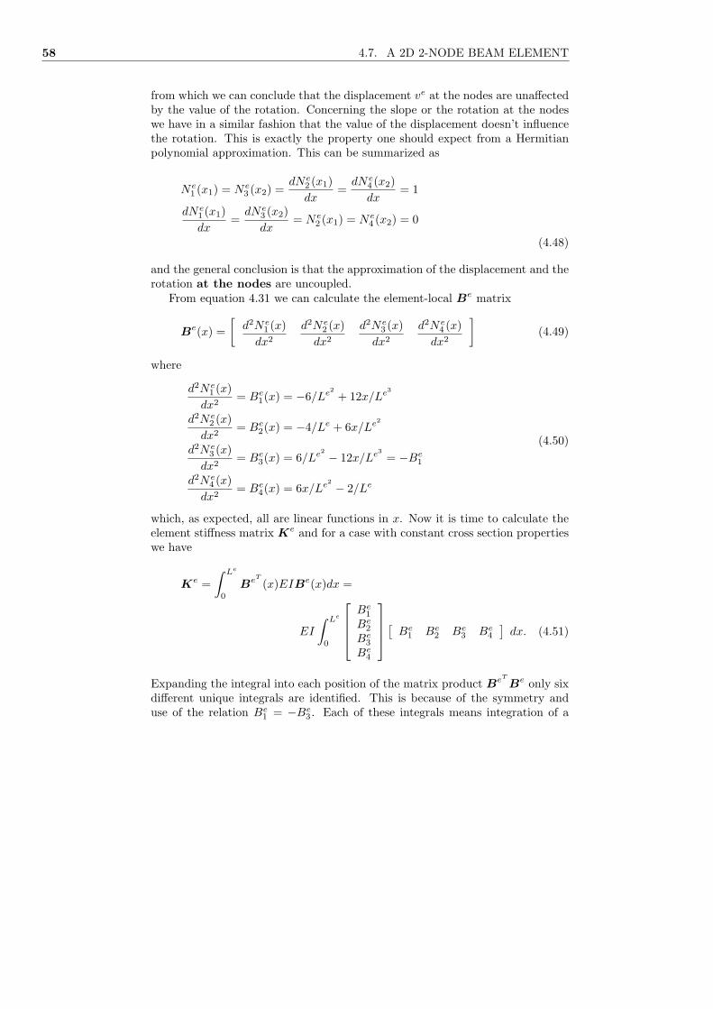
58 4.7. A 2D 2-NODE BEAM ELEMENT
from which we can conclude that the displacement ve at the nodes are unaffectedby the value of the rotation. Concerning the slope or the rotation at the nodeswe have in a similar fashion that the value of the displacement doesn’t influencethe rotation. This is exactly the property one should expect from a Hermitianpolynomial approximation. This can be summarized as
Ne1 (x1) = Ne
3 (x2) =dNe
2 (x1)dx
=dNe
4 (x2)dx
= 1
dNe1 (x1)dx
=dNe
3 (x2)dx
= Ne2 (x1) = Ne
4 (x2) = 0
(4.48)
and the general conclusion is that the approximation of the displacement and therotation at the nodes are uncoupled.
From equation 4.31 we can calculate the element-local Be matrix
Be(x) =[
d2Ne1 (x)
dx2
d2Ne2 (x)
dx2
d2Ne3 (x)
dx2
d2Ne4 (x)
dx2
](4.49)
where
d2Ne1 (x)
dx2= Be
1(x) = −6/Le2+ 12x/Le3
d2Ne2 (x)
dx2= Be
2(x) = −4/Le + 6x/Le2
d2Ne3 (x)
dx2= Be
3(x) = 6/Le2 − 12x/Le3= −Be
1
d2Ne4 (x)
dx2= Be
4(x) = 6x/Le2 − 2/Le
(4.50)
which, as expected, all are linear functions in x. Now it is time to calculate theelement stiffness matrix Ke and for a case with constant cross section propertieswe have
Ke =∫ Le
0
BeT
(x)EIBe(x)dx =
EI
∫ Le
0
Be1
Be2
Be3
Be4
[Be
1 Be2 Be
3 Be4
]dx. (4.51)
Expanding the integral into each position of the matrix product BeT
Be only sixdifferent unique integrals are identified. This is because of the symmetry anduse of the relation Be
1 = −Be3. Each of these integrals means integration of a

CHAPTER 4. BEAMS 59
second-order polynomial expression in x.
Ke = EI
∫ Le
0Be2
1 dx∫ Le
0Be
1Be2dx − ∫ Le
0Be2
1 dx∫ Le
0Be
1Be4dx
∫ Le
0Be2
2 dx − ∫ Le
0Be
1Be2dx
∫ Le
0Be
2Be4dx
∫ Le
0Be2
1 dx − ∫ Le
0Be
1Be4dx
sym∫ Le
0Be2
4 dx
(4.52)
Let us look into details concerning only the first one which is
Ke11 = EI
∫ Le
0
Be2
1 dx = EI
∫ Le
0
(− 6
Le2 +12x
Le3
)2
dx =
EI
[48x3
Le6 +26x
Le4 −72x2
Le5
]Le
0
= 12EI
Le3 (4.53)
and all the others are achieved similarly. The final result is the following 2D2-node 4-freedom beam element. This element is useless as an element to beused in beam frame works because it do not resist any axial forces.
Box: ‘2D beam element for transversal displacements only’
Ke =EI
Le3
12 6Le −12 6Le
4Le2 −6Le 2Le2
12 −6Le
sym 4Le2
This element is seldom implemented in commercial programs because it is onlyof academic interest to be used during hand calculations.
4.8 An Element Load Vector
The global load vector f has been split into 3 different parts
f = fd + fh − fg (4.54)
where the part fd consists of contributions from the distributed load q(x) whichhas to be evaluated at the element level and is given as follows
fd =n∑
i=1
CeT
i
∫ xi+1
xi
N eT
(x)q(x) dx
︸ ︷︷ ︸=f e
i
. (4.55)

60 4.8. AN ELEMENT LOAD VECTOR
where CeT
i is a Boolean matrix. This matrix defines to which global freedom eachof the element-local freedoms belongs. (For further details see the Bar chapter)
The element load vector fei can be analyzed further if we assume that the
given load q(x) at most varies as a linear function over each element interval.That is the following linear expression
q(x) = (1− x
Le)qe
1 +x
Leqe2 (4.56)
is useful where qe1 and qe
2 are the intensity of load q(x) at the nodes. This ideameans actually an ”approximation” of given data of the problem which at thefirst glance seem to be a bit stupid. What we gain from this idea is that we canproceed one further step analytically and the input to the numerical procedurewill be the load intensity at the nodes only. From an engineering point of viewone can also argue that if the given load q(x) varies rapidly with respect to xwe need to use shorter elements anyway, if we would like to try to catch detailscaused by the rapid load change.
The element load vector fei can be rewritten as
fei =
∫ Le
0
1− 3x2/Le2+ 2x3/Le3
x− 2x2/Le + x3/Le2
3x2/Le2 − 2x3/Le3
x3/Le2 − x2/Le
((1− x
Le)qe
1 +x
Leqe2
)dx (4.57)
where we have four different integrals to solve. The polynomial expressions areall at most of a fourth order degree. The result from these four integrations gives
fei =
Le(7qe1 + 3qe
2)/20Le2
(qe1/20 + qe
2/30)Le(3qe
1 + 7qe2)/20
−Le2(qe
1/30 + qe2/20)
fei =
q0Le/2
q0Le2
/12q0L
e/2−q0L
e2/12)
(4.58)
where the second expression is the special case when the load q(x) is a constant,that is qe
1 = qe2 = q0. From this we can conclude that a line load q(x) also
generate moments as well as nodal loads.
In this context one should also mention that some people argue for an adhoc reduced element load vector without nodal moments which sometimes alsois implemented in commercial programs. The treatment shown here is called aConsistent element load vector and this is what comes out from this mathematicalConsistent
element loadvector
formulation.

CHAPTER 4. BEAMS 61
Concerning the boundary condition terms fh and fg we have
fh =
0...0T0
−M0
fg =
12EIg1/Le3+ 6EIg2/Le2
6EIg1/Le2+ 4EIg2/Le
−12EIg1/Le3 − 6EIg2/Le2
6EIg1/Le2+ 4EIg2/Le
0...0
(4.59)
where these are two global load vector contributions with the same number ofrows as in the global unknown freedom vector a. Please observe that the di-mension of the terms alters between force and moment and in this discussion theessential boundary conditions occur at the left end of the beam and the naturalbc. at the right end. Several other combinations are also of course possible.
4.9 A 2D Beam Element with Axial Stiffness
In most real space frame structures it is also necessary to take axial deformationsinto account. This is, as already mentioned, not included in the previous element.Fortunately it is easy to cure this deficiency of the element. In cases with smalldeformations it is a good approximation saying that deformations in the axialand the transversal directions evolves independent of each other.
x
y, v(x)
θ1
e
v1
e v2
e
θ2
e
xi
xi+1
Element length
u1
e u2
e
Figure 4.7: A 2D 2-node frame element freedom set
That is the bar problem and the beam problem can be solved independentfrom each other using the same finite element mesh. Such a beam element re-sisting axial stiffness also is often called a Frame element Frame element

62 4.10. A 3D SPACE FRAME ELEMENT
Box: ‘2D 2-node frame element’
Ke =1Le
EA 0 0 −EA 0 012EI/Le2
6EI/Le 0 −12EI/Le26EI/Le
4EI 0 −6EI/Le 2EIEA 0 0
12EI/Le2 −6EI/Le
sym 4EI
Please observe that the sequence between the six freedoms in the element is notcritical. This selection is only one of several others which will work equally well.Most often textbooks starts, as has been done here, with the axial freedom ue
1
and continue with the two other freedoms at the first node ve1 and θe
1 and end upwith the same freedoms at the second node of the element.
Still this element lacks one important feature to be a candidate for implemen-tation in a general purpose finite element program. This 2D element stiffnessmatrix is established along a local direction and in a real space frame applicationone most likely will find members running in arbitrary directions in 2D or 3Dspace. This defect will be cured in the next section where we will discuss a 3Dbeam element in an arbitrary direction in 3D space.
4.10 A 3D Space Frame Element
To establish a general 3D beam element for any space frame analysis is ratherstraightforward. To add bending out of the plane it is just a matter of superim-posing of a second load system bending the beam in the xy-plane. For an applied
x
z
yv
2
e
u2
eu1
e
v1
e
w1
e w2
e
θz1
θz2
θy1
θy2
θx1
θx2
e
ee
e
ee
A, E, Iy , I
z , K, Le
Figure 4.8: A 3D 12-freedom beam element defined in a local system
torque trying to twist the beam the obvious choice is to use St. Venant torsionaltheory. An element stiffness matrix Ke can now easily be establish from what

CHAPTER 4. BEAMS 63
we already know, as follows
Ke =
a1 0 0 0 0 0 −a1 0 0 0 0 0b1 0 0 0 b2 0 −b1 0 0 0 b2
c1 0 −c2 0 0 0 −c1 0 −c2 0d1 0 0 0 0 0 −d1 0 0
c3 0 0 0 c2 0 c4 0b3 0 −b2 0 0 0 b4
a1 0 0 0 0 0b1 0 0 0 −b2
c1 0 c2 0d1 0 0
s y m. c3 0b3
(4.60)
where
a1 = EA/Le d1 = GK/Le
b1 = 12EIz/Le3b2 = 6EIz/Le2
b3 = 4EIz/Le b4 = 2EIz/Le
c1 = 12EIy/Le3c2 = 6EIy/Le2
c3 = 4EIy/Le c4 = 2EIy/Le
and G is the torsional modulus of the material and K is the torsional proportionalconstant for the cross section.
Remarks:
• This element works superior with respect to classical beam theory as longas the cross section has two axes of symmetry.
• In cases with open thin-walled cross sections warping of the cross sectioncan be significant and one should be careful. This typically happens incross sections where the centroid and the shear center of the cross sectiondo not coincide.
• The selected sequence between the element freedoms ae is in this case
aeT
= ue1 ve
1 we1 θe
x1 θey1 θe
z1 ue2 ve
2 we2 θe
x2 θey2 θe
z2
• One useful technique for overcoming this problem is to use shell elementfor modeling of such cross section.
We now need an element which can be used in an arbitrary direction in 3Dspace. This can be taken care of by the rules for transformation of a vector in3D space. Please note that the previous coordinate system in figure 4.8 now hasbecome a prime coordinate system or local coordinate system and the elementfreedoms present in figure 4.9 are not the same as the ones in figure 4.8.

64 4.11. STRESS AND STRAIN CALCULATIONS
x
z
y
v2
e
u2
e
u1
e
v1
e
w1
e
w2
e
θz1
θz2
θy1
θy2θ
x1
θx2
e
ee
e
ee
A, E, Iy , I
z , K, Le
x´
z´y´
Figure 4.9: A 3D global 12-freedom beam element
Let us focus on a vector u defined by components in the global coordinatesystem and the same vector now called u′ defined by components in the localcoordinate system. The relation between the components of this vectors is
u′ = Λu (4.61)
where the matrix Λ is 3x3 matrix containing direction cosines between the axesof the two systems. The transformation of the element freedom vector a′e in thelocal system to element freedoms ae defined in the global system is given by
a′e =
Λ 0 0 00 Λ 0 00 0 Λ 00 0 0 Λ
= Tae (4.62)
and this can can be used for transformation of the element-local equilibriumequation
K′ea′e = f ′e. (4.63)
where the matrix K′e is equivalent to what is called Ke in equation 4.60. Byputting equation 4.62 into equation 4.63 and multiplying with T T from the leftwe can identify a global 3D element stiffness matrix Ke and a global elementload vector fe for a beam or frame element resisting axial forces and twistingmoment and therefore useful in general 3D space frame analysis.
T T K′eT︸ ︷︷ ︸=Ke
ae = T T f ′e︸ ︷︷ ︸
=f e
(4.64)
4.11 Stress and Strain Calculations
As for bar elements and all other elements based on basically the same finiteelement formulation, the strain and the stress is calculated element by element

CHAPTER 4. BEAMS 65
at the end of the numerical analysis. We have by generalizing equation 4.2 anduse of equation 4.3
σx(x, y, z) = Eεx(x, y, z) = E
(du(x, 0)
dx− y
d 2v(x)dx2
− zd 2w(x)
dx2
)(4.65)
where the displacement component in the local y-direction is w(x) and v(x) isthe displacement in the y-direction. The first term is the axial stress due to aforce acting along the local direction of the beam. The axial and the bendingstresses together can be expressed in the element freedom vector as follows
σx(x, y, z) = E
(1Le
[ −1 1 ]
ue1
ue2
− y[
Be1 Be
2 Be3 Be
4
]
ve1
θez1
ve2
θez2
− z[
Be1 Be
2 Be3 Be
4
]
we1
θey1
we2
θey2
) (4.66)
This expression is used in the TRINITAS program for plotting of the stresslevel on the surface of every beam element.
66 4.12. NUMERICAL EXAMPLES
4.12 Numerical Examples
A 2D console beam
Let us consider a simple standard case which also has an analytical solution. Theleft end of the beam has a completely rigid support and the right end is free. Aconstant load q(x) = q0 per unit length acts along the entire length of the beam.At the right end acts a concentrated force P . That is, from a comparison withbox S we have the following values of the boundary conditions g1 = g2 = h1 = 0and h2 = P .
x
I, E, L
q0
y, v(x)P
Figure 4.10: A 2D console beam example
The exact solution to this problem is received from the Elastic curve equation4.17 which in this case can be simplified as follows
d 4v(x)dx4
= q0/EI. (4.67)
because both the cross section geometry and the material do not change alongthe beam. After integrating four times without boundaries we have
d 3v(x)dx3
= q0x/EI + C1
d 2v(x)dx2
= q0x2/2EI + C1x + C2
dv(x)dx
= q0x3/6EI + C1x
2/2 + C2x + C3
v(x) = q0x4/24EI + C1x
3/6 + C2x2/2 + C3x + C4.
Four unknown constants C1 to C4 have to be determined from the given boundaryconditions. The left end conditions g1 = g2 = 0 imply immediately that C3 =

CHAPTER 4. BEAMS 67
C4 = 0. The conditions at the right end gives
h1 = 0 ⇒ d 2v(L)dx2
= q0L2/2EI + C1L + C2 = 0
h2 = P ⇒ d 3v(L)dx3
= q0L/EI + C1 = −P/EI
C1 and C2 equal to
C1 = −P/EI − q0L/EI C2 = PL/EI + q0L/22EI
and all constants are known and the solution v(x) is
v(x) =q0L
4
24EI
(6(
x
L)2 − 4(
x
L)3 + (
x
L)4
)+
PL3
6EI
(3(
x
L)2 − (
x
L)3
).
Let us now solve this problem numerically by Finite Elements and hand calcula-tions. Use only one element with just a vertical displacement v and a rotation θin the right end. This one element problem with its left end fixed will end up inthe following two global stiffness equations describing the behavior of the consolebeam.
EI
L3
[12 −6L−6L 4L2
] vθ
=
q0L/2 + P−q0L
2/12
The two global freedoms v and θ can be calculated as follows
vθ
=
112L2
[4L2 6L6L 12
]L3
EI
q0L/2 + P−q0L
2/12
⇒
vθ
=
q0L
4/8EI + PL3/3EIq0L
3/6EI + PL2/2EI
.
From this result we can conclude that both the displacement v(x = L) and therotation θ = dv(x = L)/dx at the right end are exactly the same as from theanalytical solution above. Let us also compare the displacements along the beamat an arbitrary x-value. By use of the values of the freedoms v and θ aboveputted into the equations 4.36 and 4.46 we obtain
ve(x) = Ne3 (x)v + Ne
3 (x)θ =(3(
x
L)2 − 2(
x
L)3
) (q0L
4
8EI+
PL3
3EI
)+
((x
L)3 − (
x
L)2
)L
(q0L
3
6EI+
PL2
2EI
)
which after simplification gives
v(x) =q0L
4
24EI
(5(
x
L)2 − 2(
x
L)3
)+
PL3
6EI
(3(
x
L)2 − (
x
L)3
).

68 4.12. NUMERICAL EXAMPLES
A second important conclusion which can be drawn from this results is that thefinite element approximation in the interior of the element is exact for the partof the displacement generated by the concentrated load P but not for the partemanating from the distributed load q0. This is obvious and this conclusion couldbe drawn as a cubic polynomial was used for the beam shape function which isnot sufficient for catching the fourth order term originating from the particularsolution to the elastic curve equation for this example.
That is, in linear static elastic beam models it is enough using just one elementfor intervals without any distributed load.
If we would like to do a numerical comparison with a finite element programwe need numerical values. Use L = 1.0 m, P = 1000. N, q0 = 1000. N/m,E = 2.0 · 1011 Pa. Assume that the cross section has a height h and a width bwhere b = 4h = 0.01 m which gives the area moment of inertia I = 5.333 · 10−8
m4. At the tip of the beam we have the best agreement between this analyticalsolution and a finite element solution and from the two load systems we receive
v(x = L) = 0.01172 + 0.03125 ≈ 0.043m
from both the analytical and a finite element solution with only one element.
Displacement
Length =
x-comp. =
y-comp. =
z-comp. =
0.04297
0.
0.
0.04297
Max Axial+Bending Stress = 0.531E+09
Figure 4.11: A one element TRINITAS analysis

CHAPTER 4. BEAMS 69
4.13 Summary
After assuming that every cut perpendicular to the mean surface of the beamwill remain plane the following local equations can be stated.
Box:L ‘Local Euler-Bernoulli Beam Equations’
d2M(x)dx2
+ q(x) = 0, M(x) =∫∫
A(x)
yσx(x, y)dydz
σx(x, y) = E(x)εx(x, y)
εx(x, y) =du(x, 0)
dx− y
d 2v(x)dx2
By elimination of the moment M(x), the strain εx(x, z) and the stress σx(x, z)the following 1D fourth-order Boundary-Value problem is received.
Box: S ‘Strong form for an Euler-Bernoulli Beam’
Given q(x), h1, h2, g1 and g2. Findv(x) such that
d 2
dx2
(E(x)I(x)
d 2v(x)dx2
)− q(x) = 0 ∀ x ∈ Ω = ]0, L[
v(0) = g1 on Sg −E(L)I(L)d 2v(L)
dx2= h1 on Sh
dv(0)dx
= g2 on Sg − d
dx
(E(L)I(L)
d 2v(L)dx2
)= h2 on Sh
The following equivalent weak formulation is established after partial integrationsand restricting the weight function to be equal to zero where essential boundaryconditions are present.
Box:W ‘Weak form for an Euler-Bernoulli Beam’
Given q(x), T0, M0, g1 and g2. Findv(x) such that∫ L
0
d 2w(x)dx2
E(x)I(x)d 2v(x)
dx2dx =
∫ L
0
w(x)q(x) dx + w(L)T0 − dw(L)dx
M0
v(0) = g1dv(0)dx
= g2

70 4.13. SUMMARY
By requiring that both the approximation and the weight function are built upfrom the same set of functions a discrete Galerkin formulation is achieved.
Box:G ‘Galerkin form of an Euler-Bernoulli Beam’
Find a such that
cT (Ka− f) = cT r = 0
for every choice of the vector c (the weight function)
The single equation in the Galerkin formulation above, which shall be interpretedas a scalar product between a row vector cT and a column vector r, will nowturn over into a system of linear algebraic equations (M) because the residualvector r must be equal to a zero vector.
Box:M ‘Matrix form of an Euler-Bernoulli Beam’
Find a such that
Ka = f
where K and f are known quantities
In this beam case discussion the solution vector a to this matrix problem willcontain both displacements and rotations at the nodes.
From here the numerical procedure starts and the following work flow can beidentified.
Numerical Work Flow:
• Split the entire domain into a number of finite elements
• Define domain properties such as the Young’s modulus E, the cross sectionA and the area moment of inertia I in the elements
• Define essential boundary conditions such as fixed or prescribed node dis-placements and/or rotations
• Define natural boundary condition as given concentrated or distributedforces or moment loads
• Make a global numbering sequence of all involved unknown freedoms (Nor-mally done automatically by the program)

CHAPTER 4. BEAMS 71
• Calculate all element stiffness matrices Kei and expand and add these stiff-
ness coefficients into the appropriate positions in the global stiffness matrixK
• Calculate all element load vectors fei and expand and add these load con-
tributions into the appropriate positions in the global load vector f
• Solve the system of linear algebraic equation Ka = f by some Gauss’elimination or LR-factorization look-a-like procedure. (Further discussionsconcerning how to calculate the unknown vector a will be given later on inthe chapters to come)
• Pick up the element freedom vector aei from the global one a for one element
at the time and calculate the strains and the stresses
• Investigate the results, hopefully in terms of a nice color picture showingthe deformed structure with the stress levels in color, and try to examinethe relevance of the achieved approximation.
In most finite element analyses, after the results have been accepted from anoverall engineering point of view, one also have to accept the analysis from anumerical point of view which normally means a refinement of the mesh in somecritical part of the domain trying to find out if the accuracy of the numericalresults is sufficient.
Finally, one should not forget that the reason for doing the finite elementanalysis was some overall engineering question concerning how to design a cer-tain piece of equipment and the finite element analysis only gives some hintsconcerning the size of displacements, strains and stresses in a model of real-ity.