Finite Element Solvers: Examples using MATLAB andFEniCS

Dallas Foster

February 7, 2017

In this paper, I present a comparison between two different methods for posing and solvingFinite Element Softwares. First, two different MATLAB softwares, DistMesh and ACF, will beused to create a mesh and solve Laplace’s equation on it. Then, an introduction to the FEniCSsoftware written for C++ and Python and a few examples.

1 MATLAB Software

1.1 Mesh Generation

In order to create meshes, we use the software DistMesh [3]. The template to create the mesh is asfollows:

In [3]: % function [p,t]=distmesh2d(fd,fh,h0,bbox,pfix,varargin)

Where fd is a function defining the geometry of the object (distance function), fh is a functiondesignating the ’scaled edge length’, h0 is the initial edge length, bbox is the positions of thebounding box of the figure and pfix denotes fixed node positions desired in the mesh.

In order to create a simple circle mesh, we define:

In [16]: fd = @(p) dcircle(p, 0, 0, 1);[p, t] = distmesh2d(fd, @huniform, 0.2, [-1, -1; 1, 1], []);

For more complicated meshes, we can combine polygons by union, difference, and intersec-tion. In particular, we are interested in creating a mesh of a unit square with four circles cut out.In order to do so, we must union the four circles together, and then difference the square with thefour circles. T

In [18]: fd1 = @(p) ddiff( drectangle(p, -1, 1, -1, 1), ...dunion( dcircle(p, -0.5, 0.5, 0.3), ...dunion( dcircle(p, -0.5, -0.5, 0.4), ...dunion( dcircle(p, 0.5, -0.5, 0.3), ...dcircle(p, 0.5, 0.5, 0.4)))));

pfix = [-1, -1; -1, 1; 1, -1; 1, 1];[p1, t1] = distmesh2d(fd1, @huniform, 0.1, [-1, -1; 1, 1], pfix);

In order to fix the corners of the square, we included pfix. This fixing is necessary in order tocreate a stable mesh.

1

Simple Circle

1.2 Solver

Now that we have the mesh, we can use the ’ACF’ software package[1]. The outputs of’distmesh2d.m’ have to be preprocessed in order to be compatible with ACF. M. Peszynska haswritten ’mesh2acf.m file’ that converts the file formats and creates necessary .dat files.

In [22]: mesh2acf(p1, t1);

This file outputs files ’boundary.dat’, ’coordinates.dat’ ’elements3.dat’ that are used in the mainACF interface ’fem2d.m’. We will solve the following problem on this mesh

−∇2u = 1 u ∈ Ω

u = 0 u ∈ ∂Ω(1)

The boundary condition and right hand side are encoded in ’f.m’ and ’u_d.m’. For more informa-tion, see ACF documentation. Having all of the necessary files, we run the following command tosolve:

In [23]: run fem2d.m;

2

Square with four circles cut out

3

2 FEniCS

From the FEniCS website, "FEniCS is a popular computing platform for partial differential equa-tions (PDE)." The software is made up of numerous interfaces including DOLFIN, FFC, andMSHR. In this discussion, we will be mostly pulling from the FEniCS[2] and MSHR modules.MSHR, in particular, is helpful for building meshes based on bitwise operators. We will recreatethe examples that we had for MATLAB, and we will have additional examples afterwards in orderto showcase other aspects of the FEniCS implementation. For more information, visit the FEniCStutorial.

2.1 Mesh Generation

The beginning of any FEniCS program is the definition of the mesh. Out of the box, FEniCSprovides several basic mesh constructors. Namely, if one wanted to build a unit square mesh, ittakes two lines of python

In [1]: from fenics import *mesh = UnitSquareMesh(8,8)

In order to build more complicated meshes import the MSHR module. This module allowsyou to call an array of shapes and combine them to form complex meshes. Combining shapes isas easy as using addition and subtraction. If one wants to make an annulus, one needs only tosubtract two Circle()’s of varying radii. For example, the FEniCS code for creating the rectanglewith four missing circles is

In [9]: from mshr import *domain = Rectangle(Point(-1,-1), Point(1,1))domain -= Circle(Point(-0.5, -0.5), 0.4)domain -= Circle(Point(-0.5, 0.5), 0.3)domain -= Circle(Point(0.5, -0.5), 0.3)domain -= Circle(Point(0.5, 0.5), 0.4)mesh = generate_mesh(domain, 20)

Note that we added lines for clarity. One could just as easily define the domain in one line, sub-tracting each circle. For all of the possible bitwise operations to create a mesh, see the FEniCSdocumentation. Once the domain has been specified, then we can generate the mesh using ’gen-erate_mesh()’. The argument 20 is an indicator of the resolution of the mesh, with larger numberscreating finer meshes. More complicated meshes will be created in the Further Examples sectionof this document.

4

Square Mesh

Fenics Mesh of Square with Four Circles Removed

5

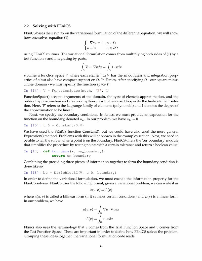
2.2 Solving with FEniCS

FEniCS bases their syntax on the variational formulation of the differential equation. We will showhow one solves equation (1)

−∇2u = 1 u ∈ Ω

u = 0 u ∈ ∂Ω

using FEniCS routines. The variational formulation comes from multiplying both sides of (1) by atest function v and integrating by parts.∫

Ω∇u · ∇vdx =

∫Ω1 · vdx

v comes a function space V where each element in V has the smoothness and integration prop-erties of u but also have compact support on Ω. In Fenics, After specifying Ω - our square minuscircles domain - we must specify the function space V .

In [14]: V = FunctionSpace(mesh, 'P', 1)

FunctionSpace() accepts arguments of the domain, the type of element approximation, and theorder of approximation and creates a python class that are used to specify the finite element solu-tion. Here, ’P’ refers to the Lagrange family of elements (polynomial) and 1 denotes the degree ofthe approximation to be linear.

Next, we specify the boundary conditions. In fenics, we must provide an expression for thefunction on the boundary, denoted uD. In our problem, we have uD = 0

In [15]: u_D = Constant(0.0)

We have used the FEniCS function Constant(), but we could have also used the more generalExpression() method. Problems with this will be shown in the examples section. Next, we need tobe able to tell the solver when a point is on the boundary. FEniCS offers the ’on_boundary’ modulethat simplifies the procedure by testing points with a certain tolerance and return a boolean value.

In [17]: def boundary(x, on_boundary):return on_boundary

Combining the preceding three pieces of information together to form the boundary condition isdone like so

In [18]: bc = DirichletBC(V, u_D, boundary)

In order to define the variational formulation, we must encode the information properly for theFEniCS solvers. FEniCS uses the following format, given a variational problem, we can write it as

a(u, v) = L(v)

where a(u, v) is called a bilinear form (if it satisfies certain conditions) and L(v) is a linear form.In our problem, we have

a(u, v) =

∫Ω∇u · ∇vdx

L(v) =

∫Ω1 · vdx

FEnics also uses the terminology that u comes from the Trial Function Space and v comes fromthe Test Function Space. These are important in order to define how FEniCS solves the problem.Grouping these ideas together, the variational formulation code reads

6

Solution to Poisson Equation on mesh

In [22]: u = TrialFunction(V)v = TestFunction(V)f = Constant(1.0)a = dot(grad(u), grad(v))*dxL = f*v*dx

Finally, we can solve the problem implementing a, L, u, and the boundary conditions.

In [23]: u = Function(V)solve(a == L, u, bc)

7

3 Further Examples

In order to showcase some other features of the FEniCS meshing and solving aparatus, we presentthe following two examples. First, a solution to Laplace’s equation on an irregular domain withmultiple Dirichlet boundary conditions. Second, a 3-dimensional problem heat equation problem.

3.1 Laplace Equation with Irregular Annular Domain

We would like to solve the following problem−∇2u = 0 u ∈ Ω = ΓO ∪ ΓI ∪ ΓE

u = 0.15 u ∈ ΓO

u = 0.8 u ∈ ΓI

u = 0.55 u ∈ ΓE

(2)

Where we define ΓO,ΓI ,ΓE in the mesh code below. As we did above, the first step to solving thisproblem is to create the mesh

In [31]: domain = Circle(Point(0,0), 1)-Circle(Point(0,0), .25)domain -= Circle(Point(0,1), .4)domain -= Ellipse(Point(-0.7, 0), 0.25, 0.45)domain -= Circle(Point(0.75, 0.4), 0.3)mesh = generate_mesh(domain, 20)

# Define Function Space:V = FunctionSpace(mesh, 'P', 2) # Quadratic

Next, we create the boundary functions. Care is taken in order to ensure that the appropriatevalues are taken where specified. In particular, we use the FEniCS near() function to determineif a point is close to the boundary. Since we have more than one boundary condition, we mustcombine them somehow. Luckily, FEniCS makes it easy to put each boundary condition into onesingle python array that we can pass to the solver.

Annulus Mesh

8

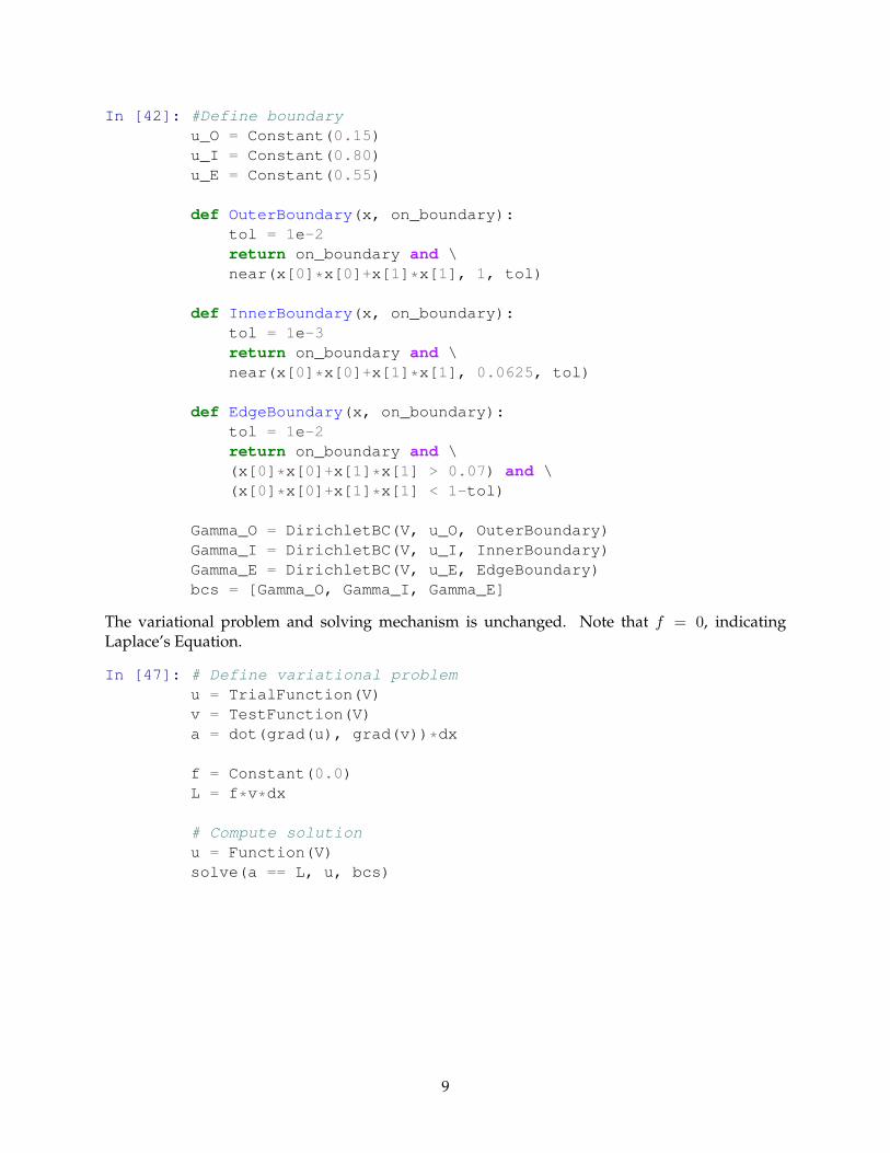
In [42]: #Define boundaryu_O = Constant(0.15)u_I = Constant(0.80)u_E = Constant(0.55)

def OuterBoundary(x, on_boundary):tol = 1e-2return on_boundary and \near(x[0]*x[0]+x[1]*x[1], 1, tol)

def InnerBoundary(x, on_boundary):tol = 1e-3return on_boundary and \near(x[0]*x[0]+x[1]*x[1], 0.0625, tol)

def EdgeBoundary(x, on_boundary):tol = 1e-2return on_boundary and \(x[0]*x[0]+x[1]*x[1] > 0.07) and \(x[0]*x[0]+x[1]*x[1] < 1-tol)

Gamma_O = DirichletBC(V, u_O, OuterBoundary)Gamma_I = DirichletBC(V, u_I, InnerBoundary)Gamma_E = DirichletBC(V, u_E, EdgeBoundary)bcs = [Gamma_O, Gamma_I, Gamma_E]

The variational problem and solving mechanism is unchanged. Note that f = 0, indicatingLaplace’s Equation.

In [47]: # Define variational problemu = TrialFunction(V)v = TestFunction(V)a = dot(grad(u), grad(v))*dx

f = Constant(0.0)L = f*v*dx

# Compute solutionu = Function(V)solve(a == L, u, bcs)

9

Annulus Solution

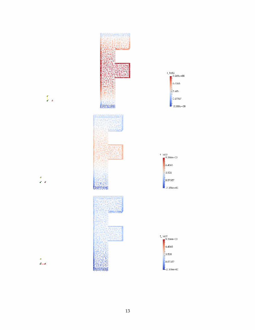
3.2 Heat Equation 3-D

Let Ω = ΓD ∪ ΓN . We would like to solve the heat equation∂u∂t = ∇2u+ f u ∈ Ω× [0, T ],

u = uD u ∈ ΓD × (0, T ],

u = uN u ∈ ΓN × (0, T ],

u = u0 at t = 0.

(3)

The solution to this problem will be similar to the other examples in many ways. We must createa mesh and appropriate variational formulation. New to this problem, being time-dependent, wemust integrate using finite-difference over the temporal domain. We can set up the T-domain likeso

In [66]: T = 20.0 # Final Timesteps = 50dt = T/steps

The mesh used in this example is three dimensional. MSHR provides many methods, but wecombine several Box()’s to create an F.

In [53]: domain = Box(Point(0, 0, 0), Point(1, 5, 1))+Box(Point(1, 4, 0), Point(2, 5, 1))domain += Box(Point(1, 2, 0), Point(2, 3, 1))mesh = generate_mesh(domain, 40)

# Define Function SpaceV = FunctionSpace(mesh, 'P', 1)

10

fmesh

Now, we set up the boundary conditions. For our problem, we assume that there is constantheat flux at the top - uT - and bottom - uB - of our F. The other faces will be subject to Neumannboundary conditions that are accounted for in the variational formulation.

In [72]: u_T = Constant(2.0)u_B = Constant(-2.0)def Top_boundary(x, on_boundary):

tol = 1e-2return on_boundary and (x[1]>(5-tol))

def Bottom_boundary(x, on_boundary):tol = 1e-2return on_boundary and (x[1]<tol)

bc1 = DirichletBC(V, u_T, Top_boundary)bc2 = DirichletBC(V, u_B, Bottom_boundary)bcs = [bc1, bc2]

We must be precise when we develop the variational formulation in order to take care of the time-dependence of the problem. Let us discretize the time domain. Let tn and un denote the time andvalue of u and at the nth time step respectively. Then at the tn+1 time step, we have(

∂u

∂t

)n+1

= ∇2un+1 + fn+1

We can approximate the time derivative using the backward euler scheme:(∂u

∂t

)n+1

≈ un+1 − un∆t

where ∆t is the time step. Substituting the approximation gives

un+1 − un∆t

= ∇2un+1 + fn+1

11

If we multiply both sides of the above equation by a test function v and integrate by parts, we canwrite this equation in the form

a(u, v) = Ln+1(v)

wherea(u, v) =

∫Ω+∆t

∫Ω∇u · ∇vdx

andL(v) =

∫Ω(un +∆tfn+1)vdx+

∫ΓN

∆t(uN )nvds

Now that we have our equation properly formulated, we can construct our problem.

In [74]: u_n = interpolate(u_0, V)f = Expression('exp(-pow(x[0]-0.5, 2)-pow(x[1]-2.5, 2)- pow(x[2]-0.5,2))/(1+t)', degree=1, t=0)u_N = Expression('sin(t)', degree=1, t=0)

u = TrialFunction(V)v = TestFunction(V)a = u*v*dx+dt*dot(grad(u), grad(v))*dxL = (u_n+dt*f)*v*dx - dt*u_N*v*ds

Because we have a time dependent problem, we must solve our problem at each time discretiza-tion. The total solution is computed in the following for loop.

In [75]: u = Function(V)t = 0vtkfile = File('heatequationf.pvd')for n in range(steps):

t+=dtf.t = t #update fu_N.t = t #update u_Nsolve(a == L, u, bcs)u_n.assign(u) #update u_n!

12

13

References

[1] J. ALBERTY, C. CARTENSEN, AND S. A. FUNKEN, Remarks around 50 lines of matlab: short finiteelement implementation.

[2] M. S. ALNÆS, J. BLECHTA, J. HAKE, A. JOHANSSON, B. KEHLET, A. LOGG, C. RICHARDSON,J. RING, M. E. ROGNES, AND G. N. WELLS, The fenics project version 1.5, Archive of NumericalSoftware, 3 (2015).

[3] P.-O. PERSSON AND G. STRANG, A simple mesh generator in matlab, SIAM Review, 46 (2004),pp. 329–345.

14