Embed Size (px)
Citation preview

FINITE ELEMENT SIMULATION
OF
FLAT NOSE LOW VELOCITY IMPACT BEHAVIOUR
OF
CARBON FIBRE COMPOSITE LAMINATES
A THESIS SUBMITTED
TO
THE UNIVERSITY OF BOLTONIN PARTIAL FULFILLMENT OF
THE REQUIREMENTS FOR
THE DEGREE OF DOCTOR OF PHILOSOPHY
BY
UMAR FAROOQ
June 2014

Umar Farooq ii
In the Name of Allah: The Most Gracious, The Most Merciful-who showed the right path of
righteousness and blessed me to get the strength to embark upon this task of peeping into
the realms of facts and events. His blessings have always support and nurtured author’s
goals and principles in life.

Umar Farooq iii
Abstract
The work detailed in this thesis includes an extensive finite element simulation of low
velocity impact behaviour of carbon fibre reinforced laminated composite panels subjected
to flat and round nose impacts.
Carbon fibre composites are being widely used in aerospace structures due to their high
strength and stiffness ratios to weight and potential to be tailored for structural
components. However, wing and fuselage skins are vulnerable to foreign object impacts
during manufacturing and service from tools maintenance tools and tool box drops. Such
impacts particularly from flat nose tool drops inflict internal damages that are difficult to
detect through routine inspections. The internal damage (barely visible) may cause severe
degradation of material properties and reduction in compressive strength that might lead
in unexpected catastrophic failures. Such failures result in loss of human lives and
structural assets. That is a major concern for the aircraft industry. Most of the existing
research is based on damage detection and control to improve integrity of structures so
that an aircraft could reach nearest safe place to avoid failure after damage is detected.
It is very difficult to evaluate overall structural congruity and performance as structural
degradation and damage progression occur after impacts. The impact is a dynamic event
which causes concurrent loading and re-distributions of stresses once a ply fails or damage
occurs. Most of the reported studies are based on physical experiments which are
expensive, time consuming, and limited. The efficient way to predict performance
evaluation of an impacted structural component is through integrated computer codes that
couple composite mechanics with structural damage and failure progressions.
Computational models can be very useful in simulating impact events, interpreting results,
and making available the fast predictive tools for pre-design analysis and post-impact
damage evaluations.
This investigation is primarily simulation based that integrates experimentally and
numerically evaluated impact response of laminates manufactured by AircelleTM Safran Ltd
and HexcelTM Composites. Literature review and basic mathematical formulations relevant
to the impact of composite laminates were commented. Pre-assumed damage induced
static load-deflections simulation using “PTC Creo SimulateTM” were carried out for eight,

Umar Farooq iv
sixteen, and twenty four ply laminates subjected point, low, medium, and large nose
impacts. The methodology used was based on previous experimental studies that assumed
that impact damage provides the same stress concentration effect as crack, regions of
degraded materials, or softer inclusions. The same assumptions were incorporated into
simulation by inserting pre-assumed damage zones equivalent to impactors’ nose tips with
within the volume of the laminates. Damage initiation, growth, and accumulation were
investigated in terms of real scenarios with reference to the undamaged specimens. Several
internal damage mechanisms were analysed via damage shift in multiple locations
throughout the laminates’ volumes. The simulations can be useful to predict and correlate
information on: existence, type, location, and extent of the damage in the impacted system
to applied load. With this information and the loads applied to the system, measures can be
proposed to reduce adverse effects of the impact induced damage.
The compressive residual strength after impact was predicted via buckling simulation
models. The in-plane buckling analysis was implemented into PTC Creo SimulateTM. Effects
of the pre-assumed damage ply, damage zone, and coupled damaged-ply with damage zone
were investigated via through-thickness re-locations. Critical buckling load and mode
shapes were predicted with reference to the mid-surface of the laminates. Local buckling
was simulated by introducing damage in a single ply adjacent to surface of the sub-
laminate. Cases of pre-assumed delaminated ply from top to the mid-surface were
simulated. Cases of mix-mode buckling analysis were simulated from coincident and
combined effects of pseudo damaged ply as well as damage zones. The simulations
predicted information can be useful to predict useful life remains (prognosis) of the
damaged system. The information could also be useful to predict residual strength of
similar cases at the beginning from material level, loading scenarios, damage progression to
component and system level at various rates.
Material property characterization tests were conducted to verify the industry provided
input and used in drop-weight impact simulations. The properties were augmented with
micro-macro mechanics formulations to approximate full range of engineering constants
from reliably determined Young’s modulus. The drop-weight simulation of eight, sixteen,
and twenty four ply specimens of quasi-isotropic lay-ups having different thicknesses and
impacted from round and flat nose impactors were implemented in the ABAQUSTM software

Umar Farooq v
using explicit dynamic method. Two independent models were implemented in the
software. The first model simulates displacement, velocity, and acceleration quantities. The
second model computes in-plane stresses required to efficiently evaluate 3D stresses. The
in-plane stress quantities were numerically integrated through-the-thickness utilising
equilibrium to evaluate ply-by-ply through-thickness stresses. The evaluated stress values
were then utilised in the formulation set of advanced failure criteria to predict damage
progression and failure modes.
Simulation produced results were compared and verified against experiment produced
data. Drop-weight impact tests were conducted to verify the selected simulation produced
results. Non-destructive techniques and advanced data filtering algorithms available in
MATLABTM were utilised to filter the noisy data and predict damage zone and load
threshold. The selected simulation results were compared against the experimental data,
intra simulation results, and the results available in the literature and have to agree up to
90%.
The investigation concludes that the simulation models could efficiently predict low
velocity impact response of variety of carbon fibre composite panels that could be useful
for design development with reduced testing.

Umar Farooq vi
Acknowledgements
Completing a thesis such as this requires the understanding and assistance of a great many
people. The author cannot hope to name all the individuals who have assisted him along the
way but wishes to pay tributes to many people without whom this achievement would not
have been possible.
The most importantly, the author owes his deepest gratitudes to Alightly Allah (SWT) for
His continuous blessing throughout bumby journey of his life where dreams come true.
First of all sincere appreciations and gratitudes go to Prof Dr Peter Myler for his
encouragement, valuable time, and ability to guide excellently throughout this endeavour.
Moreover, for the person he is, his vision and knowledge are only surpassed by his
generous personality. Those who have had the privilege of interacting with him will agree
that he is a teacher and a fried. The author has had the privilege of working with such a
highly reputed professor. Many thanks go to Prof Dr Baljinder K Kandola and Dr Gerard
Edwards for being author’s co-supervisors and for their many fruitful and constructive
comments during discussions and presentations.
The author particularly thanks to Mr Zubair Hanslot and Mr Karl Gregory for their excellent
teaching of finite element analysis, computer aided design, and computational modelling
courses. Particular thanks go to Miss Charly Slyter, Mr William Hales, Mr Sathish Kiran
Nammi, and Mrs Sravanthi Nowpada for their help and assistance with working on
commercial software in Design Studio. Special thanks go to Mr. Akbar Zarei of Centre for
Material Research and Innovation for all the help and support with experimental work on
INSTRONTM impact tester and Universal Material Testing machines.
The author cannot forget to thank his all time well wishers and senior ex-colleagues Prof Dr
Muhammad Alam, Prof Dr G F Tariq, Prof Dr Afzaal Malik, Prof Dr Farahad Ali, Dr
Muhammad Tariq, Prof DR T M Shah, and Ch M Naseem of Government Degree College
Kahuta Rawalpindi in Pakistan for their guidance and support during his stay there. The
author also feels indebted to his colleages Prof Dr Yousaf Khan, Mr Amanullah Baloch, and

Umar Farooq vii
Mr Mushtaq Yaqubai along with his numerical analysis studentsat Hazara University
Mansehra in Pakistan for their support during his service there.
The author will also remain grateful to numerous investigators and everyone who helped,
supported, and contributed to the development of this body of knowledge.
The author would like to profoundly acknowledge The University of Bolton for providing
him the study opportunity with excellent learning facilities. The author would also like to
acknowledge and thank to HexcelTM Composites and AircelleTM Safran Limited for
donations of the carbon composite panels used in this research. Research interest on flat
nose drop-weight impact behaviour of carbon composite panels by the staff from British
Aerospace Engineering Systems, Salisbury, is greatly appreciated and acknowledged.
The author would like to acknowledge contributions of the faculty and staff of Composite
Certification Laboratories of Manchester University and Electronic Department of Bolton
University for their help with Ultrasonic C-scan and Eddy-Current testing of impacted
panels. The author is thankful to Prof Dr John Milnes of the Fire Laboratory of Bolton
University for his help with ignition loss testing to determining engineering properties of
the panels. The author would also like to extend his gratitude’s to Mr Jason Bolton for his
help with manufacturing purpose-built flat nose impactors and assistance with the
workshop work.
At last but not least, the author would like to thank all his family members here in the
United Kingdom and his disable sister in Pakistan and wished that his mother were still
alive to see this work completed. During all those years their loves and prayers have been
source of inspiration. Their blessings have always stayed beside the author.

Umar Farooq viii
Table of Contents
Acknowledgements ................................................................................................................. vi
List of Figures ......................................................................................................................... xv
List of Tables .......................................................................................................................... xxi
Chapter 1 Introduction ............................................................................................................. 1
1.1. Introduction ................................................................................................................ 1
1.2. Fibre reinforced laminated composites ...................................................................... 1
1.3. Foreign object impacts of composites and internal damage ...................................... 3
1.4 Statement of the problem ........................................................................................... 6
1.5 Methodologies to study low velocity impact on composites ..................................... 6
1.5.1 Experimental methods and issues .............................................................................. 6
1.5.2 Analytical methods and limitations ........................................................................... 7
1.5.3 Computational modelling methods ............................................................................ 8
1.6 Motivations and need for computational modelling .................................................. 8
1.7 Selection of computational modelling methodology ................................................. 9
1.8 Goals and objectives of the study .............................................................................. 9
1.9 Contribution of the investigation ............................................................................. 12
1.10 Organization of the thesis ........................................................................................ 13
Chapter 2 Literature review ................................................................................................... 16
2.1 Review ..................................................................................................................... 16
2.2 Fibre-reinforce composites and low velocity impact damage ................................. 16
2.3 Impact damage resistance of composite laminates .................................................. 18
2.4 Impact damage tolerance of composite laminates ................................................... 19
2.4.1 Global buckling analysis .......................................................................................... 19
2.4.2 Local buckling analysis............................................................................................ 20
2.4.3 Mixed mode buckling analysis ................................................................................ 20
2.5 Properties determinations of composite laminates .................................................. 21
2.6 Simulation of drop-weight low velocity impact of laminates .................................. 22
2.7 Low velocity impact testing of laminates and damage diagnostics ......................... 24
2.8 Data filtering and extrapolation of test generated data to predict damage .............. 29
2.9 Summary .................................................................................................................. 30
Chapter 3 Strength and deformation of fibrous composites under impact ....................... 32

Umar Farooq ix
3.1 Review ..................................................................................................................... 32
3.2 Modelling impact of composite laminates ............................................................... 32
3.2.1 Static load-deformation ............................................................................................ 33
3.2.2 Impact dynamic analysis .......................................................................................... 36
3.3 Influence of impactor’s nose shape and loading area .............................................. 37
3.4 Residual strength from buckling analysis ................................................................ 39
3.5 Selection of finite element simulation methodology ............................................... 41
3.6 Summary .................................................................................................................. 42
Chapter 4 Load-deflection simulation using PTC Creo SimulateTM software ..................... 43
4.1 Review ..................................................................................................................... 43
4.2 Laminates, impactor nose profiles, and material properties .................................... 43
4.2.1 Laminates and impactors ......................................................................................... 43
4.2.2 Material properties of undamaged and damaged laminates ..................................... 44
4.3 Selection of methodology and software ................................................................... 46
4.3.1 The load-deflection methodology ............................................................................ 46
4.3.2 The commercial software PTC Creo SimulateTM
.................................................... 47
4.4 Developing static load-deflection computational model ......................................... 47
4.5 Static load-deflection predictions of undamaged laminates .................................... 49
4.5.1 Approximation of damage shapes corresponding to impactor nose profiles ........... 49
4.5.2 Comparison of simulated and experimental results ................................................. 50
4.5.3 Comparison of simulated results for flat and round nose impactors ....................... 51
4.5.4 Influence of loading area influence to undamaged laminates .................................. 53
4.5.5 Influence of partitioned loading area to undamaged laminates ............................... 54
4.5.6 Selection of the pre-assumed damage methodology ................................................ 56
4.6 Simulation of pre-assumed damage induced load-deflection .................................. 58
4.7 Discussion of the simulation generated results ........................................................ 60
4.7.1 Impactor nose shape against lay-up sequence ......................................................... 60
4.7.2 Influence of damage locations ................................................................................. 63
4.7.3 Impactor nose on against successive damage zone and loading area ...................... 65
4.8 Impactor nose shape against through-thickness damage location ........................... 70
4.8.1 24-Ply laminate ........................................................................................................ 70
4.8.2 16-Ply laminate ........................................................................................................ 72
4.8.3 8-Ply laminate .......................................................................................................... 74
4.9 Summary .................................................................................................................. 76
Umar Farooq x
Chapter 5 Residual strength prediction using PTC Creo SimulateTM software .................. 78
5.1 Review ..................................................................................................................... 78
5.2 Methodology for buckling analysis ......................................................................... 78
5.2.1 Determination of buckling load of the sub-laminate ............................................... 78
5.2.2 Determination of buckling load of laminated plate ................................................. 81
5.3 Pre-assumed de-lamination induced buckling analysis ........................................... 86
5.3.1 Finite element meshing schemes ............................................................................. 87
5.3.2 Simulation of un-damaged laminate ........................................................................ 92
5.3.3 Simulation of damaged laminate ............................................................................. 93
5.4 Validation of selected buckling analysis methodology ........................................... 95
5.4.1 Influence of pre-assumed de-laminated zone on buckling load ............................... 95
5.4.2 Influence of delamination depth (location) on buckling load .................................. 96
5.5 Comparison of intra-simulation results .................................................................... 98
5.5.1 Constant sized pre-assumed delaminated zone ........................................................ 98
5.5.2 Increasing pre-assumed damage zones .................................................................. 100
5.5.3 Symmetric and un-symmetric lay-ups ................................................................... 101
5.6 Numerical results and discussions ......................................................................... 103
5.6.1 Global buckling analysis ........................................................................................ 103
5.6.1.1 Simulation of hole laminate ............................................................................... 103
5.6.1.2 Damaged ply at various locations ...................................................................... 105
5.6.2 Local buckling analysis.......................................................................................... 108
5.6.2.1 Single pre-assumed damaged zone at various locations .................................... 109
5.6.2.2 Multiple pre-assumed damaged zone at various locations ................................ 112
5.6.2.3 Switching of local and global buckling modes .................................................. 113
5.7 Mixed-mode buckling simulation .......................................................................... 114
5.8 Summary ................................................................................................................ 118
Chapter 6 Determination of physical and mechanical properties .................................... 120
6.1 Review ................................................................................................................... 120
6.2 Determination of properties ................................................................................... 120
6.3 Determination of physical properties ..................................................................... 121
6.4 Determination of elastic properties of a lamina (Rule of Mixture) ....................... 122
6.5 Engineering constants for orthotropic lamina in 2D .............................................. 126
6.6 Engineering constants in 3D .................................................................................. 131
6.7 Engineering constants for quasi-isotropic laminate ............................................... 136

Umar Farooq xi
6.8 Determining elastic constants from flexure theory ................................................ 138
6.9 Experimental methods to determine mechanical properties .................................. 140
6.9.1 Tensile test ............................................................................................................. 141
6.9.2 Flexural test ............................................................................................................ 143
6.9.2.1 Young’s modulus based on load-displacement measurements .......................... 146
6.9.2.2 Young’s modulus based on strain measurements .............................................. 146
6.9.2.3 Young’s modulus based on slope measurements............................................... 147
6.9.3 Hart Smith rule ....................................................................................................... 148
6.9.4 Determining effective moduli for laminated composites....................................... 149
6.10 Summary ................................................................................................................ 152
Chapter 7 Simulation of drop-weight impact using ABAQUSTM software ........................ 154
7.1 Review ................................................................................................................... 154
7.2 Theoretical aspects of the contact-impact for low velocity impact ....................... 154
7.3 Simplified modelling of impact problem using contact law .................................. 156
7.3.1 Implicit method ...................................................................................................... 159
7.3.2 Explicit method ...................................................................................................... 162
7.4 Materials and geometric properties of laminates and impactors ........................... 167
7.5 Experimental testing and computer simulation of drop-weight impacts ............... 170
7.5.1 Impact test facility ............................................................................................ 170
7.5.2 Impact test procedure ...................................................................................... 173
7.6 Comparison of results for flat and round nose impactor .................................. 176
7.6.1 Experimental results of 8-Ply laminate at 1.7 m/s velocity ......................... 176
7.6.2 Comparison of damage evaluation through velocity parameter .................. 177
7.6.3 Experimental and simulated results ............................................................... 177
7.6.4 Comparison of the results through delaminated zone ratios ....................... 178
7.7 Theoretical aspects of stress-based methodology ............................................ 183
7.7.1 Determination of forces and moments at mid-plane .............................................. 184
7.7.2 Effect of Poisson’s ratios on through-thickness stresses ....................................... 186
7.7.3 Determination of through-thickness stresses ......................................................... 189
7.8 Failure theories for impacted composite laminates ............................................... 191
7.8.1 Failure prediction using limits criteria ................................................................... 192
7.8.1.1 Maximum stress criteria (limit theory) .............................................................. 192
7.8.1.2 Maximum strain criteria (energy conservation) ................................................. 192

Umar Farooq xii
7.8.2 Interactive polynomial criteria ............................................................................... 193
7.8.3 Mode base failure criteria ...................................................................................... 194
7.9 Material properties and plan of simulations using ABAQUSTM
software ............. 196
7.9.1 Simulation models with sweeping meshes ............................................................ 196
7.9.2 Adaptive meshing techniques ................................................................................ 197
7.10 Discussion based on intra-simulation results .................................................... 199
7.10.1 Impact of 8-Ply laminate .................................................................................. 199
7.10.1.1 Impact velocity 1.7 m/s ............................................................................... 199
7.10.1.2 Impact velocity 2.2 m/s ............................................................................... 201
7.10.2 Impact of 16-Ply laminate................................................................................ 204
7.10.3 Impact of 24-Ply laminate................................................................................ 208
7.11 Summary ............................................................................................................... 212
Chapter 8 Low velocity impact of composite laminates .................................................... 214
8.1 Review ................................................................................................................... 214
8.2 Carbon fibre reinforced laminates and type of impactors ...................................... 214
8.3 Drop-weight impact test methodology................................................................... 214
8.3.1 Impact testing plan ................................................................................................. 215
8.4 Non-destructive damage detection techniques ....................................................... 216
8.4.1 Visual inspections .................................................................................................. 217
8.4.2 Eddy-current (electromagnetic induction) ............................................................. 218
8.4.3 Ultrasonic c-scans techniques ................................................................................ 219
8.5 Comparison of results ............................................................................................ 220
8.5.1 Damage assessment of 8-Ply laminates ................................................................. 220
8.5.2 Damage assessment of 16-Plylaminates ................................................................ 224
8.5.3 Damage assessment of 24-Plylaminates ................................................................ 226
8.5.4 Prediction of impact induced damage area ............................................................ 228
8.5.5 Laminates of different material properties ............................................................. 231
8.5.5.1 8-Ply laminate impacted at velocity 1.7 m/s ...................................................... 231
8.5.5.2 16-Ply laminate impacted at velocity 3.12 m/s .................................................. 231
8.5.5.3 24-Ply laminate impact energy: 20 J, 30 J, and 50 J .......................................... 232
8.6 Limitations associated with testing and non-destructive techniques ..................... 233
8.7 Theoretical determination of impact parameters ................................................... 234
8.7.1 Parameters that affect the impact response ............................................................ 235

Umar Farooq xiii
8.7.2 Parameters determined from impact test generated data ....................................... 235
8.7.2.1 Forces, mass and acceleration ............................................................................ 235
8.7.2.2 Energy balances (virtual work and d’Alembert’s principle) .............................. 236
8.7.2.3 Energy absorbed by target ................................................................................. 237
8.7.2.4 Determination of contact duration ..................................................................... 241
8.7.3 Comparison of load-deflection and drop-weight impact results ............................ 243
8.7.4 Parameters determined from quasi-static load testing ........................................... 244
8.8 Delamination threshold load determine from facture mechanics .......................... 247
8.8.1 Threshold load of single delamination ................................................................... 248
8.8.2 Threshold load of multiple delaminations ............................................................. 252
8.9 Influence of impactor nose shape .......................................................................... 253
8.9.1 Backface strain under point nose impact ............................................................... 253
8.9.2 Backface strain under flat nose impact .................................................................. 255
8.9.3 Critical threshold load under flat loading .............................................................. 258
8.9.4 Threshold load associated with ring loading ......................................................... 260
8.9.5 The second threshold load associated with back face cracking ............................. 261
8.10 Summary ................................................................................................................ 263
Chapter 9 Analysis of test generated data ........................................................................... 265
9.1 Review ................................................................................................................... 265
9.2 Selection of data filtering and data extrapolation techniques ................................ 265
9.3 Data filtering based on built-in filters (data acquisition system) ........................... 268
9.3.1 8-Ply laminate impacted at different velocities ..................................................... 268
9.3.2 8-Ply laminate impacted from different nose profiles ........................................... 268
9.3.3 Energy history for 8-Ply laminate .......................................................................... 269
9.3.4 Comparison of load, displacement, velocity, and deflection history ..................... 270
9.3.5 Limitations of the built-in filters ............................................................................ 271
9.4 Data filtering using statistical (moving average) methods .................................... 273
9.4.1 16-Ply laminate comparison of impact velocity and impactor nose ...................... 274
9.4.2 16-Ply laminate energy history .............................................................................. 275
9.4.3 Comparison of load, displacement, velocity, and deflection history ..................... 276
9.4.4 Load and energy for different lay-ups ................................................................... 277
9.4.5 Higher order moving average methods .................................................................. 277
9.4.6 Limitations of the statistical (moving average) filters ........................................... 278
9.5 Data filtering using numerical techniques ............................................................. 278

Umar Farooq xiv
9.5.1 16-Ply and 24-Ply laminate prediction of energy .................................................. 280
9.5.2 Comparison of load, displacement, velocity, and deflection history ..................... 284
9.5.3 16-Ply and 24-Ply laminates versus flat and round nose impactors ...................... 284
9.5.4 Limitations of the filters based on numerical techniques ...................................... 285
9.6 Data filtering and extrapolation using Fast Fourier algorithms ............................. 285
9.6.1 Fast Fourier algorithms as filters ........................................................................... 285
9.6.2 Energy history for 24-Ply laminate ........................................................................ 290
9.6.3 16-Ply and 24-Ply laminates versus flat and round nose impactors ...................... 291
9.6.4 Comparison of load, displacement, velocity, and deflection history ..................... 293
9.6.5 Validation of the results obtained using Fast Fourier filters .................................. 297
9.6.5.1 Validation against available data ....................................................................... 297
9.6.5.2 Validation of the results against statistical filter ................................................ 298
9.6.5.3 Validation of the results against mean value filter............................................. 299
9.7 Summary ................................................................................................................ 300
Chapter 10 Conclusions and recommendations for future work ...................................... 303
10.1 Review ................................................................................................................... 303
10.2 Summary of each chapters’ conclusions ................................................................ 303
10.3 Major contribution of the investigations ................................................................ 306
10.3.1 Influence from flat nose shape impactors .......................................................... 307
10.3.2 Efficient prediction of through-thickness stresses and failure modes ............... 307
10.3.3 Damage prediction through data filtering and data extrapolation ..................... 308
10.3.4 Recommendations for future investigations ...................................................... 308
Appendix: Selected publications ......................................................................................... 325
Appendix A Journals .......................................................................................................... 325
Appendix B Conferences.................................................................................................... 327

Umar Farooq xv
List of Figures
Figure 1-1: Superior properties: widely used in aircraft industry ....................................... 2
Figure 1-2: Evolution of composite usage in aircraft structures [2] .................................... 3
Figure 1-3: Foreign object drop-weight impact threat ......................................................... 3
Figure 1-4: Schematic of low velocity impact and common damage modes [3] ................. 4
Figure 1-5: Various failure modes at different scales [5]. ..................................................... 5
Figure 2-1: Micro-macro mechanical analysis model ......................................................... 17
Figure 2-2: Integration techniques function of strain-rate [129]. ..................................... 25
Figure 2-3: Typical trapezoidal distribution of damage in laminates [133] ..................... 26
Figure 2-4: Frequency range for ultrasonic application [144] ........................................... 28
Figure 3-1: General laminate symmetrical about its middle-plane ................................... 32
Figure 3-2: Forces and moments acting on a plate .............................................................. 33
Figure 3-3: Local and global axes of matrix and rotated fibres .......................................... 36
Figure 3-4: Differential element positions for buckling analysis ....................................... 40
Figure 3-5: Common finite element simulation process of engineering problems. ......... 42
Figure 4-1: Schematic of: a) fibre orientation, b) laminate, and c) circular cut-out ......... 44
Figure 4-2: Schematic of impactor noses with nose diameters .......................................... 44
Figure 4-3: A typical pre-processed meshed model for 24-Ply laminate .......................... 48
Figure 4-4: Typical computer generated damage resistance models ................................ 49
Figure 4-5: Photographs: a) front surface and b) close up image ...................................... 49
Figure 4-6: C-scanned images of: a) 8-Ply, b) 16-Ply, and c) full size 24-Ply laminate .... 50
Figure 4-7: Comparison of 8-Ply laminate impacted by impact nose 2.1 mm. ................. 51
Figure 4-8: Simulated contours of 8-Ply laminates: a) flat and b) round nose. ................ 52
Figure 4-9: Simulated 8-Ply laminate: a) legend table and b) stress contours [4]. .......... 52
Figure 4-10: Images show damage in red colour ................................................................ 53
Figure 4-11: Deflection against radius of loading area ...................................................... 55
Figure 4-12: Deflection against radius of loading area ...................................................... 55
Figure 4-13: Deflection against radius of loading area ...................................................... 56
Figure 4-14: Overlapping zones a) single, b) two, and c) Three........................................ 58
Figure 4-15: Static load-deflection analysis flowchart........................................................ 60
Figure 4-16: Deflection v location of damage ply for 8-Ply at nose 6.3 mm ..................... 64
Figure 4-17: Deflection v loading area for 8-Ply at nose 6.3 mm ...................................... 64
Figure 4-18: Deflection v loading area for 24-Ply laminate 3 noses .................................. 66
Umar Farooq xvi
Figure 4-19: Deflection v loading area for 24-Ply laminate 3 noses .................................. 67
Figure 4-20: Deflection v loading area for 24-Ply laminate 3 noses .................................. 68
Figure 4-21: Deflection v loading area for 24-Ply laminate 3 noses .................................. 69
Figure 4-22: Deflection against damage location 24-Ply laminate v impactor nose ....... 71
Figure 4-23: Deflection against damage location for16-Ply laminate v impactor nose ... 73
Figure 4-24: Deflection against damage location for8-Ply laminate v impactor nose .... 75
Figure 5-1: Schematic representation (1) sub-laminate and 2) column). ......................... 79
Figure 5-2: Bending and compression acting on a delaminated orthotropic plate: a)
Theoretical, b) Local buckling, and c) Global buckling modes ..................................... 82
Figure 5-3: Finite element model representation ............................................................... 88
Figure 5-4: Undamaged a) schematics and b) finite element model ................................. 90
Figure 5-5: a) Un-meshed, b) Course meshed, c) Mapped mesh, d) Fine meshed, and e)
Loaded and fine meshed ................................................................................................. 92
Figure 5-6: Double delamination simulation at the mid-plane [1] .................................... 94
Figure 5-7: Single delamination simulation at the mid-plane [1] ...................................... 94
Figure 5-8: Residual strength v damaged zone (a) and b) Simulated ................................ 96
Figure 5-9: Buckling load v through-thickness location (a) and b) Simulated) ................ 97
Figure 5-10: Schematics of 8-, 16-, and 24-ply specimens.................................................. 99
Figure 5-11: Buckling load v location of de-laminated zone diameter (mm) ................. 100
Figure 5-12: Buckling load v damage zone for 8-, 16- & 24-Ply laminate ....................... 100
Figure 5-13: Buckling load v damage zone ........................................................................ 101
Figure 5-14: Buckling load v through-thickness location damage area .......................... 102
Figure 5-15: Flowchart for damage tolerance analysis..................................................... 103
Figure 5-16: Schematics of laminate embedded within a hole......................................... 104
Figure 5-17: Increasing pre-assumed damage zone against buckling load KN .............. 105
Figure 5-18: Schematic of; a) damage ply and b) ply location ......................................... 105
Figure 5-19: Buckling load against damage location of ply in 8-Ply laminate ................ 106
Figure 5-20: Buckling load against damage location of ply in 16-Ply laminate .............. 107
Figure 5-21: Buckling load against damage location of ply in 24-Ply laminate .............. 107
Figure 5-22: Symmetric 8-Ply laminate: a) hole and b) damage ...................................... 108
Figure 5-23: Buckling load against pre-assumed damage diameter: 20 mm .................. 109
Figure 5-24: Buckling load against pre-assumed damage diameter zone: 40 mm ......... 110
Figure 5-25: Buckling load against pre-assumed damage diameter: 60 mm .................. 110
Umar Farooq xvii
Figure 5-26: Buckling load against pre-assumed damage diameter: 80 mm .................. 111
Figure 5-27: Buckling load against pre-assumed damage diameter: 100 mm ............... 111
Figure 5-28: Case 1: Buckling load against multiple damage for 24-Ply laminate ......... 112
Figure 5-29: Case 2: Buckling load against multiple damage for 24-Ply laminate ......... 113
Figure 5-30: Local buckling turns to global buckling (damage location effect) .............. 114
Figure 5-31: Schematics of mixed-mode buckling model ................................................. 115
Figure 5-32: Buckling load against damage location for8-Ply laminate .......................... 116
Figure 5-33: Buckling load against damage location for16-Ply laminate ........................ 116
Figure 5-34: Buckling load against damage location for24-Ply laminate ........................ 117
Figure 6-1: Flowchart of determining physical and mechanical properties ................... 121
Figure 6-2: Stresses in an isotropic lamina under a plane stress condition. ................... 126
Figure 6-3: Orthotropic lamina in a plane stress ............................................................... 127
Figure 6-4: Coordinate systems referred to 3D transformation relations. ..................... 134
Figure 6-5: Schematic of pure flexure of beam .................................................................. 138
Figure 6-6: Schematic of beam laminates with cross-section .......................................... 141
Figure 6-7: Photographs of: a) laminate and b) INSTRONTM machine ............................ 142
Figure 6-8: Schematics: a) laminate bending and b) cross-sectional area ...................... 144
Figure 6-9: a) Test laminate b) test chamber .................................................................... 145
Figure 6-10: Progression of micro-macro analysis ........................................................... 151
Figure 7-1: Load-deflection response a) Static and b) Dynamic ...................................... 155
Figure 7-2: Impactand local-global deformation ............................................................... 157
Figure 7-3: Time step and stress wave relationship ......................................................... 165
Figure 7-4: 8-Ply symmetric laminates .............................................................................. 167
Figure 7-5: a) 8-ply, b) 16-ply, and c) 24-ply specimens .................................................. 168
Figure 7-6: a) Schematic of a) specimen, b) cut-out of impact affected zone; c) round
nose , and d) flat nose shape impactors ....................................................................... 169
Figure 7-7: Flowchart of drop-weight impact analysis ..................................................... 170
Figure 7-8: INSTRONTM 9250HV impact test machine ...................................................... 173
Figure 7-9: Images of C-scanned 8-Ply laminates impacted at 1.7 m/s velocity ............ 176
Figure 7-10: Comparison of 8-Ply laminates subjected to flat and round impactors [4].
......................................................................................................................................... 177
Figure 7-11: Comparison of 8-Ply laminates subjected to flat and round impactors. .... 178
Figure 7-12: Mesh grid projected on 8-Ply C-Scanned laminate [4] ................................ 179

Umar Farooq xviii
Figure 7-13: Selected C-Scan images and Eddy-current surfaces [4] ............................. 182
Figure 7-14: Comparison of 24-Ply laminate damage pattern [4] ................................... 183
Figure 7-15: Coordinate locations of ply in a laminate ..................................................... 185
Figure 7-16: Coordinate system and layer positions defined in a laminate .................... 189
Figure 7-17: Computer generated meshed models and stack of 8-Ply laminate [4] ...... 197
Figure 7-18: Computer generated impact models: a) Flat nose b) Round impactors .... 198
Figure 7-19: Top-ply in-plane stresses Pa of 8-Ply laminate at velocity 1.7 m/s [4]. .... 200
Figure 7-20: Failure index based on ply-by-ply through-thickness stresses ................. 201
Figure 7-21: Top ply in-plane stresses (Pa) of 8-Ply laminate at velocity 2.2 m/s [4] ... 202
Figure 7-22: Failure index based on ply-by-ply through-thickness stresses .................. 203
Figure 7-23: Failure index based on ply-by-ply through-thickness stresses .................. 203
Figure 7-24: Top ply in-plane stresses Pa of 16-Ply laminate at velocity 3.12 m/s [4] . 205
Figure 7-25: Failure index based on ply-by-ply through-thickness stresses .................. 206
Figure 7-26: Failure index based on ply-by-ply through-thickness stresses .................. 207
Figure 7-27: Top ply in-plane stresses Pa of 24-Ply laminate at 3.12 m/s [4] ................ 209
Figure 7-28: Top ply in-plane stresses Pa of 24-Ply laminate at velocity 4 m/s [4]....... 210
Figure 7-29: Failure index based on ply-by-ply through-thickness stresses .................. 211
Figure 7-30: Failure index based on ply-by-ply through-thickness stresses .................. 211
Figure 8-1: Image of impacted laminate: a) front and b) back surfaces .......................... 217
Figure 8-2: Eddy current testing ......................................................................................... 218
Figure 8-3: Schematic of the ultrasonic equipment .......................................................... 219
Figure 8-4: C-scan images and Eddy-current surface ....................................................... 221
Figure 8-5: Simulated images and legend tables from ABAQUSTM software ................... 222
Figure 8-6: C-scan images and Eddy-current surface ....................................................... 223
Figure 8-7: C-scan images and Eddy-current surface ....................................................... 224
Figure 8-8: C-scan images and Eddy-current surface ....................................................... 225
Figure 8-9: Simulated images and legend tables from ABAQUSTM software ................... 226
Figure 8-10: C-scan images and Eddy-current surface ..................................................... 226
Figure 8-11: C-scan images and Eddy-current surface ..................................................... 227
Figure 8-12: Simulated images and legend tables from ABAQUSTM software ................ 228
Figure 8-13: Comparison of 24-Plylaminate C-scan and Eddy-current images. ............. 229
Figure 8-14: C-scan image of 8 J impact using the round impactor ................................. 232
Figure 8-15: C-scan images using flat impactor................................................................. 232

Umar Farooq xix
Figure 8-16: Load-time history of flat and round nose impacts. ...................................... 234
Figure 8-17: Static-indentation against drop-weight (filtered) at load 3.2 KN .............. 243
Figure 8-18: Static-indentation against drop-weight (filtered) at load 8.9 KN .............. 244
Figure 8-19: Load, energy and displacement hemispherical impact response. .............. 245
Figure 8-20: Load, energy and displacement flat impact response. ................................ 246
Figure 8-21: Load, energy and displacement hemispherical impact response. .............. 247
Figure 8-22: Delamination induced simply supported axis-symmetrical plate ............. 248
Figure 8-23: Load-history of 8-Ply laminate under round nose impact scale................. 249
Figure 8-24: Load, absorbed energy histories 34.5 J hemispherical impact [1]. ............ 251
Figure 8-25: Nomenclature for exact and approximate solution ..................................... 254
Figure 8-26: Schematic of 3-point beam bending of symmetric plate ............................. 254
Figure 8-27: Nomenclature for the integrated ring-loaded exact solution. .................... 255
Figure 8-28: Clamped plate under variable load at radius rp (from 0 to a). .................... 259
Figure 8-29: Clamped plate under ring/annular load ....................................................... 260
Figure 8-30: Clamped plate under central circular uniform load .................................... 262
Figure 9-1: Schematic of projected multiple damage onto a single plane ...................... 265
Figure 9-2: Schematic of possible damage modes [21]. .................................................. 266
Figure 9-3: Flowchart depicting stages of present work................................................. 267
Figure 9-4: Load-deflection response of 8-Ply laminates................................................ 269
Figure 9-5: Energy-history plot of 8-Ply laminate round and flat nose impactors ......... 269
Figure 9-6: a) Velocity, load and deflection histories; flat nose compared to b)........... 270
Figure 9-7: a) Velocity, load and deflection history; round nose against b). ................. 271
Figure 9-8: Load deflection comparison of 8-Ply laminate at velocity 1.7 m/s. ............ 271
Figure 9-9: Load-deflection comparison of 8-Ply response at velocity 1.6 m/s ............. 272
Figure 9-10: Load-deflection plot of 16-Ply laminate; round and flat impacts. ............. 274
Figure 9-11: Load-deflection of 16-Ply laminate; round and flat nose impactors. ........ 274
Figure 9-12: Energy-histories of 16-Ply laminate at velocity 3.12 m/s .......................... 275
Figure 9-13: Velocity, load and deflection of 16-Ply laminate; velocity 3.12 m/s. ........ 276
Figure 9-14: Load, energy history of 16-Ply and 24-Ply laminate responses. ............... 277
Figure 9-15: Load, energy history of 16-Ply response with high order filter. ............... 278
Figure 9-16: Numerical filter and extrapolation relations................................................ 279
Figure 9-17: Load, velocity and deflection of 24-Ply laminate at velocity 3.74 m/s. .... 284
Figure 9-18: Schematics of Fourier filter process. ............................................................ 287

Umar Farooq xx
Figure 9-19: Energy history of 24-Ply laminate impacted at velocity 3.74 m/s. ........... 291
Figure 9-20: Load-deflection of 16-Ply at velocity 3.74 m/s ............................................ 292
Figure 9-21: Load-deflection of 24-Ply laminate at velocity 3.74 m/s ............................ 292
Figure 9-22: Velocity, load and deflection of 24-Ply laminate; a) and b) round ............ 293
Figure 9-23: Velocity, load and deflection of 24-Ply laminate; a) flat & b) round ......... 294
Figure 9-24: Load-deflection plot of 24-Ply laminate filtered using Fast Fourier .......... 296
Figure 9-25: Load-deflection plot of 24-Ply laminate filtered using Fast Fourier .......... 296
Figure 9-26: Load-deflection threshold load 10 KN validates 8.9 KN. ............................ 298
Figure 9-27: Load-deflection plot validates predicted load 24 KN against 23 KN in ..... 298
Figure 9-28: Load-deflection comparison to predict threshold loads ............................. 299
Figure 9-29: Load-deflection comparison to predict threshold loads ............................. 300

Umar Farooq xxi
List of Tables
Table 4-1: Properties of laminate and impactor [1] ............................................................ 45
Table 4-2: Degraded material properties for pre-assumed damage zone ........................ 46
Table 4-3: Loading areas mm2............................................................................................... 54
Table 4-4: Schematics of damaged ply and damaged areas mm2 ...................................... 57
Table 4-5: Approximation of net damage zones .................................................................. 58
Table 4-6: 8-Ply laminate simulated under impactor nose diameter 2.1 mm .................. 61
Table 4-7: 8-Ply laminate simulated under impactor nose diameter 4.2 mm .................. 62
Table 4-8: 8-Ply laminate simulated under impactor nose diameter 6.3 mm .................. 63
Table 4-9: Top ply of 24-Ply laminate under impactor nose 6.3 mm ................................ 65
Table 4-10: Top-ply 24-Ply laminate under impactor nose 6.3 mm .................................. 67
Table 4-11: Top-ply 24-Ply laminate under impactor nose 6.3 mm .................................. 68
Table 4-12: Top-ply 24-Ply laminate under impactor nose 6.3 mm .................................. 69
Table 5-1: Ply-by-ply local buckling load KN ....................................................................... 81
Table 5-2: Results of theoretical calculated buckling load ................................................. 85
Table 5-3: Results of theoretical calculations based on Eq. (5-24) .................................... 86
Table 5-4: Ply-by-ply local buckling load (KN) .................................................................... 98
Table 6-1: Measured geometrical properties..................................................................... 122
Table 6-2: Fibre contents of laminate of code Fibredux 914c-833-40. .......................... 122
Table 6-3: Beams lay-up configuration and geometrical dimensions ............................. 142
Table 6-4: Tensile test results ............................................................................................. 143
Table 6-5: Formulation used to calculate young’s modulus. ............................................ 144
Table 6-6: Formulation used to calculate young’s modulus. ............................................ 146
Table 6-7: Strain based calculated young’s modulus. ....................................................... 147
Table 6-8: Modulus based calculated young’s modulus. ................................................... 147
Table 6-9: Young’s modulus for Fibredux 914C-833-40................................................... 148
Table 6-10: Young’s modulus determined from Hart Smith Rule .................................... 149
Table 6-11: Number plies and their weight factors in a laminate ................................... 150
Table 6-12: Lay-up, angle, and modulus of 8-Ply laminate .............................................. 150
Table 6-13: Comparison of Young’s moduli determined from various methods ........... 151
Table 7-1: Material B properties [4] ................................................................................... 168

Umar Farooq xxii
Table 7-2: Test plan of the selected simulation cases ....................................................... 178
Table 7-3: Algorithm approximating the delaminated area [4] ....................................... 180
Table 7-4: Comparison of delaminated ratios [4].............................................................. 181
Table 8-1: Impact testing plan............................................................................................. 216
Table 8-2: Drop-weight impacted laminate against damage zone ................................... 230
Table 8-3: Estimated values proportionate to thickness .................................................. 257
Table 9-1: An example of three-point moving average method ....................................... 273
Table 9-2: Code for modified Simpson rule ....................................................................... 281
Table 9-3: numerical integration to estimate area under the curve ................................ 282
Table 9-4: numerical integration to estimate area under the curve ................................ 283
Table 9-5: Comparison of energy values ............................................................................ 283
Table 9-6: Time domain decomposition of 16 point data through 4 stages ................... 289
Table 9-7: Roots of unity and periodic symmetry ............................................................. 290
Table 9-8: Code to compute Discrete Fourier Transforms ............................................... 294
Table 9-9: Code to compute fast Fourier Transforms ....................................................... 295
Table 9-10: Code for extrapolation ..................................................................................... 297

Umar Farooq xxiii

Chapter 1 Introduction
Umar Farooq 1
Chapter 1 Introduction
1.1. Introduction
This thesis reports computational and experimental investigation conducted on low
velocity impact damage resistance and impact damage tolerance of carbon fibre composite
laminates subjected to round and flat nose impacts. The work is a logical progression and
extension of the work undertaken and compiled by James [1] which focused on the
experimental data and testing fixture design. The thesis work shows qualitative agreement
in the predicted and observed damage patterns and residual strength. While a great deal of
efforts in the research areas have been directed towards the experimental
characterizations, an efficient and accurate computational model for the prediction of
impact damage behaviour of composites is still lacking. This is a consequence of the three
dimensional nature of impact damage and complexity of the geometry of internal damage
and delamination of composites. The work herein is aimed to develop an efficient
computational model using finite element based software to efficiently handle the three-
dimensional aspects that includes through-thickness stresses. The through-thickness
stresses are then utilised in mode-based advanced failure criteria to predict matrix
cracking and ply-by-ply delamination characteristics at ply interfaces.
1.2. Fibre reinforced laminated composites
Carbon fibre composites were developed by combining two or more engineering materials
reinforced with strong material fibres to obtain a useful third material that displays better
mechanical properties and economic values. Most of the composite materials are made by
stacking several distinct layers of unidirectional lamina or ply. Each lamina or ply is made
of the same constituent materials, matrix and fiber, The Figure 1-1 shows evolution of
carbon composites from fibre and matrix to structural applications in aerospace, civil, and
military applications.

Chapter 1 Introduction
Umar Farooq 2
Figure 1-1: Superior properties: widely used in aircraft industry
The composites are being widely used as structural elements in aerospace structures due to
their high ratios of strength and stiffness to weight and flexibility features to tailor part
integration and buckling resistance essential to structural stability. The heavier structural
assemblies are being replaced by composites to enhance safety and saving in fuel
consumptions. Market for the composites’ applications as structural element is constantly
growing in aerospace, sport, automobile, civil and military applications. The BoeingTM 787
Dreamliner and AirbusTM 350 Extra Body Wide (XWB) and A380 are already utilising up to
50% carbon fibrous composites by weight as shown in Figure 1-2 [2].

Chapter 1 Introduction
Umar Farooq 3
Figure 1-2: Evolution of composite usage in aircraft structures [2]
1.3. Foreign object impacts of composites and internal damage
The composites offer great potential in characteristic flexibilities which make them more
versatile in tailoring structural components. However, wings and fuselages are situated
such that they are particularly exposed to maintenance tools (tool boxes) drops regarded as
flat nose impact that inflicts internal damage as shown in Figure 1-3.
Figure 1-3: Foreign object drop-weight impact threat
The low velocity impact is a simple event that occurs when an impactor hits a target but
does not penetrate the target. In case of impact on laminated composites it has many
complicated effects. Impact induced damage is difficult to detect by routine inspections, the

Chapter 1 Introduction
Umar Farooq 4
internal damage mode initiates by intra-ply matrix cracking which grows and results in
delamination that leads in fibre breakage as shown in Figure 1-4 with severe reduction in
residual strength.
Figure 1-4: Schematic of low velocity impact and common damage modes [3]
(1) The impact induced coupled damage could reduce residual strength as much as
65% [1] during future compressive loading that might end-up in un-expected
catastrophic failures resulting in loss of human lives and financial loss to the
airliners. The other aspect of the investigation is that the full potential offered by
composite materials is not being utilised. The current allowable design for strain
failure is in the range of 0.3% to 0.4% [1], [2], and [3] while common undamaged
laminates fail in excess of 1.2 to 1.5 % strain [4]. The existing design allowable
requires increased safety factor that leads to over-designed components which are
un-necessarily heavier than required. As a consequence, enormous uncertainties
arise in design procedures to ensure that structure containing damage will not fail
(exceed allowable strain limits) under the design ultimate load. This leads
applications of high safety factors and a strongly over-dimensioned design in the
end. Another aspect is that, it is very difficult to evaluate overall structural
performance once damage occurred: as stresses re-distribute and damage grows
after impacts. Failure prediction for laminates with pre-assumed damaged zones
(cutouts) is considerably more difficult than failure prediction of un-notched
lamina. This is due in part because of the 3D state of stress that can affect failure.
Inter-laminar shear and inter-laminar normal components present in the state of
stress cannot be neglected. In addition, localized subcritical damage in the highly

Chapter 1 Introduction
Umar Farooq 5
stressed region may occur. As local damage on the microscopic level occurs in the
form of fibre pull-out, matrix micro-cracking, fiber-matrix interfacial failure, matrix
serrations and/or cleavage, and fiber breakage. On the macroscopic level, damage
occurs via matrix cracking, delamination, and failures of individual plies. These
localized damage mechanisms act to reduce damage (notch) sensitivity and increase
the part strength. Brian Esp. reported some of the failure modes and their coupling
in flowchart as shown in [5] Figure 1-5.
Figure 1-5: Various failure modes at different scales [5].
To improve impact damage resistance and damage tolerance have always been an issue of
concern due to the inherent difficulties of elastic brittle laminated composite materials with
complicated damage mechanisms. Generally recognised and accepted analysis method is
currently not available to predict impact damage resistance and damage tolerance [33].
This requires detailed investigations and understanding of the low velocity impact
behaviour of composite laminates.

Chapter 1 Introduction
Umar Farooq 6
1.4 Statement of the problem
Accidental drop of low velocity and heavy mass tool or tool box on the aircraft wing and
fuselage skin is common occurrence that cannot be avoided. Aircraft industry resorts to
experimental analyses where components are being over designed to operate with
significant impact damage. Analytical studies based on three-dimensional laminated plate
theories are oversimplified that neglect contribution from through-thickness stresses. The
round nosed impactors are mainly used to study impact on aircraft structure. However, a
real impact is not likely to be from round nose shape. Impact from the flat nose shape
impactor causes internal invisible damage under similar impact conditions that is a major
concern for aircraft industry. Major concern is the inability to predict actual compressive
residual strength from growth of internal damage. No standard experimental method exists
to correlate impact load to the resulting damage and residual strength. Detailed
investigations to study response of the composite laminates subjected to flat and round (for
comparison) nose impactors are not reported in the available literature. Hence,
computational model to characterise flat impact events that include contributions from
through-thickness stresses to aid in prediction of damage formation and its effect on
structural performance is required.
1.5 Methodologies to study low velocity impact on composites
Extensive experimental, analytical, computer simulations are underway to enhance inherit
potential of composites in their applications and to minimise risks from the foreign object
impact. Investigations are based on identifying common occurring damage scenarios and to
concentrate on detection and elimination of damage without falling strength and stiffness
of impacted components to unacceptable levels.
1.5.1 Experimental methods and issues
The experimental methods rely on a large number of tests in real-size structural
components that consume huge efforts and resources. New applications are frequently
emerging and testing methods need to be modified to accommodate the specific
engineering requirements. In most of the cases the traditional methods are becoming
incapable in analysing the new materials and require costly development and replacement

Chapter 1 Introduction
Umar Farooq 7
of physical equipment. At times, it is not feasible to test all vulnerable surfaces of an aircraft
with increasing needs of on-line inspection and continuous assessment of aircraft’s health
condition while in service. Standard test methods capable of predicting the remaining life of
impact damaged structural element are not available. Moreover, existing mechanical tests
are not always able to reproduce all the circumstances of environmental conditions,
loadings, interactions, combinations and damage diagnostics that may encounter during an
aircraft’s service life. Involvement of a large number of variables in the impact event, data
scatting and variations in test result comparisons from one program to the others are also
issues.
1.5.2 Analytical methods and limitations
Analytical methods can be applied to many simple aspects to meet the ever increasing
demands of understanding the impact behavior of composites. The methods turn the
impact event into mathematical model using mechanics of composites based on the
elasticity theory have proven to possess acceptable accuracy for relatively simple
applications. However, general three-dimensional elasticity solutions are not available for
the impact responses of laminated composites. The structural characteristics of anisotropy,
heterogeneity, the existence of matrix and fibre interface with different properties and
presence of the manufacturing defects pose difficulties in development of constitutive
models for analytical studies to assist structural designs. Moreover, impact is a dynamic
event which causes concurrent loading and re-distributions of stresses once a ply fails or
damage occurs. As composites are anisotropic materials, the rate-dependent constitutive
equations cannot be readily obtained. Most of the analytical analyses on the topic are based
on ‘quasi-static indentation’ which relies on in-plane, linear, and small deflection applying
‘classical laminated plate theory’. In the quasi-static analysis influence of dynamic effects
and through-thickness stresses (regarded major source of failure) are neglected[36]. The
simplified analytical methods lack in reliable analysis of three dimensional dynamic low
velocity impacts of composites.

Chapter 1 Introduction
Umar Farooq 8
1.5.3 Computational modelling methods
A large number of computational models have been developed based on the classical
laminated plate theories. However, most of the studies are over simplified and based on
three-dimensional solid elements that consume large computing resources. Major
shortcomings of the existing analyses are neglecting of the through-thickness stresses that
make failure and damage modes difficult to identify despite number of proposed failure
criteria. Moreover, most of the existing studies use single scale mesh discretisation scheme
over the entire domain for multi-layer structural element. This produces unnecessary
excessive number of degrees of freedom mainly in the regions which are located at far
distances from the impact zone where there is no need for such high level of details and
resolution with fine scale meshing. Such discretisation processes result in large
computation time and over-burdening of the available computing resources. The impact
event is generally a local phenomenon that requires a fine-scale meshing of the high stress
gradient regions within the computational domain to capture material and geometrical
nonlinear effects. While the regions located outside of the impact vicinity do not go through
such nonlinear effects mesh refinement and a relatively coarse mesh can be adopted.
1.6 Motivations and need for computational modelling
Prediction of damage resistance and tolerance has become a design focus as aircraft
certification requires structural capability to carry the ultimate load until the next
scheduled inspection. No recognised unified experimental approach is available to correlate
ply-by-ply internal damage and failure to the applied load. Consequently, designers rely on
ad-hoc determining structural performance. This approach is not satisfactory as the use of
data recorded from ad-hoc performance may result in either under-designed or over-
designed structures. Understanding of impact on composite structures has always been an
issue of concern, principal causes for loss of structural integrity, and reasons why
composites have not achieved their full potential and widespread usage. Most of the
reported relevant studies are experimentally based, expensive, time consuming, and
limited. The most effective way to obtain performance evaluation estimates of structural
components is through integrated computer codes that couple composite mechanics with
structural damage and failure progressions. Due to the cost and limitations of testing
methods, many industries have already adopted virtual analysis for the majority of simple

Chapter 1 Introduction
Umar Farooq 9
problems using computer simulations. The verification tests are being conducted at the end
of the design processes. The huge computing power integrated with data and signal
processing techniques and state-of-the-art software can be utilised to develop an efficient
and reliable simulation model. The computing aids are also very useful in interpreting and
comparing results. It thus becomes important to develop a computational model that could
predict flat nose low velocity impact response of composites relatively efficiently for pre-
design analysis.
1.7 Selection of computational modelling methodology
Simulation models based on PTC Creo SimulateTM and ABAQUSTM finite element software
were developed. The software codes are capable to discretise the computational domain
with nonlinear effects. Moreover, the explicit codes in ABAQUSTM are generally employed
for numerical solution of impact problems due to their dynamic and highly nonlinear
nature. The built-in features of the software options have the potential to serve and can be
utilized with various levels of complexity and mechanical responses to independently mesh
the sub-domains. The computational models can be very useful for a viable virtual design
capability that allows parametric studies for validating the numerical results. The
generated data could be useful for material selection purposes and possibly to make a pre-
design (approximate) proposal of the impact performance of similar structural components
with enhanced confidence in damage tolerance capabilities. The model can be modified to
generate data from simulation of simple scenarios of operational structural components for
comparison against experimentally recorded data.
1.8 Goals and objectives of the study
Motivated by the above statements six main goals were set to accomplish the
investigations:
(a) To search and select literature regarding solution methods to the low velocity
impact of composites
(b) Develop static load-deflection and buckling analysis models utilising PTC Creo
SimulateTM software to validate selected results from the available quasi-static and
compression after impact tests [1].

Chapter 1 Introduction
Umar Farooq 10
(c) Perform extended pre-assumed damage/delaminated zone simulations predicting
ply-by-ply static load-deflection and buckling analyses.
(d) To determine and verify properties of carbon fibre laminates used in the analysis
(e) To implement the drop-weight impact event by flat and round nose impactors in
ABAQUSTM software using efficient meshing schemes to simulate load-deflection model
to predict elastic failure
(f) To develop stress based model to predict in-plane stresses to numerically integrate
the 2D stresses via equilibrium equations to predict 3D stresses and to use them in
advanced failure theories
(g) To conduct drop-weight experimental testing and predicting damage and
delamination prediction using non-destructive techniques data interpretation and
extraction techniques.
To achieve the goals, the objectives given below were set to:
(1) Develop static load-deflection finite element models to generate and correlate data to
the pre-assumed damage zones against deflection. Cases of damage locations and sizes
need to be simulated for:
a) Eight, sixteen, and twenty-four ply laminates
b) Pre-assumed damage corresponding to point, small, medium, and large impactor
nose shapes
c) Relocations of the pre-assumed damage within volumes of laminates
d) Investigations of loading effects by partitioning loading areas under impactor nose
profiles
e) Develop buckling analysis model to capture compressive residual strength after
impact. The simulations need to be carried out for:
i) Local buckling analysis
ii) Global buckling analysis.
iii) Mixed mode buckling analysis.
(2) Design and conduct property characterisation experiments to verify laminates
properties used in the investigations. To determine and verify properties of carbon
fibre laminates used in the analysis:
a) Physical properties from ignition loss tests
b) Mechanical properties from tensile and bending tests

Chapter 1 Introduction
Umar Farooq 11
c) Rule of mixture and Hart Smith rule
d) Micro-mechanics and mechanics of composites formulations
(3) Develop an independent model to predict load-deflection from flat and round nose
impacts to capture the dynamic effects of an impact load for:
a) To simulate load-deflection model
b) To simulate stress based model to predict in-plane stresses
c) To determine through-thickness (3D) stresses utilising the computed
in-plane (2D) stresses by numerical integrating equilibrium
equations through-thickness
d) To predict ply-by-ply failure utilising the in-plane and through-
thickness stresses in advanced failure criteria.
(4) Design and conduct drop-weight impact experiments on composite laminates to
predict damage using non-destructive techniques for:
a) Damage and delamination prediction using non-destructive
techniques and impact parameters using theoretical formulations
b) Interpretation and extraction of damage and load drops (threshold
load) using data filtering and data extrapolation of test generated
data
c) Comparisons and validation of drop-weight simulation generated
and quasi-static results
(5) Draw conclusions regarding the validity of investigated results and techniques
commonly used in the literature. Provide outcome of the integrated simulation
analysis supported by experimental and analytical results consisting of the flat nose
impact response of the composite laminates.
Tasks described in goals were incorporated in commercially available software to develop
solution models. Simulations and physical tests were carried out and selected results were
validated and compared against the data available in the literature. Moreover, material
properties were verified. All objectives of the investigations were met in this research
work. Corresponding to the investigations, ten chapters from I to X were prepared.
Chapter 1 Introduction
Umar Farooq 12
1.9 Contribution of the investigation
This investigation contributes in efforts towards efficient and reliable design analysis of the
flat nose impact damage resistant and damage tolerant of composites. Capabilities of
capturing internal damage and degradation via simulation significantly contribute in
economic and performance benefits in the following aspects:
(1) To efficiently predict flat nose impact induced through-thickness stresses from two-
dimensional simulations and utilise them to predict mode based failures. Through-
thickness ply-by-ply failures, damage modes, and damage mechanisms occur in
service life of an aircraft can be predicted efficiently. The simulation produced
results can be useful to evaluate and provide resistance ability to a structural part at
pre-design stage.
(2) Simulation predicts and measures sufficient static strength using pre-assumed
embedded damage zones correlation to deflection quantities. The information can
be useful to correlate damage detecting abilities and resistance to potential impact
damage threats. Predicts damage resistance of components to maintain statistical
design strength by correlating against undamaged (as is) components.
(3) To predict residual strength of laminate embedded with possible damaged and
delaminated zones. Such predictions correlate ability of the laminates at pre-design
stage to tolerate presence of the anticipated damage and possess adequate
structural integrity. Simulations can be useful in predicting damage tolerance
capabilities without physical testing of many components under ultimate loads.
(4) Physical and mechanical properties determined from tests can be augmented with
relevant calculations and formulations to determine enhanced using micro-macro
mechanics laws.
(5) Non-destructive damage detection techniques can be complemented with
mathematical formulation to determine unknown parameter from known
parameters without further testing. Moreover, the data filtering and data
extrapolation techniques can be utilised to interpret damage through load
fluctuations.

Chapter 1 Introduction
Umar Farooq 13
1.10 Organization of the thesis
The thesis is structured in ten chapters corresponding to the progression of the research.
The chapters are organized as follows:
Chapter I introduce investigation topic, motivation, primary aim and objectives, and
contributions of the investigations, and indicate organization of the thesis.
Chapter II provides a literature review in the relevant aspects of laminated composites
impacted from various impactor nose profiles with information on references.
Chapter III outlines relevant theory associated with the impact of composite plates
applicable to this research: load-deflection, drop-weight impact, buckling analyses and
failure theories.
Chapter IV deals with the simulation model developed on the basis of load-deflection
methodology in “PTC Creo SimulateTM” software. Various test cases of pre-assumed ply-by-
ply damage laminates, impactor nose profiles, and stacking sequences were investigated.
Pre-assumed damage zones were correlated to simulation produced deflection quantities.
Selected results were compared to the available experimental results.
Chapter V consists of simulation of compressive-bending buckling analysis to predict
residual strength of the damaged laminates. Independent models were developed for local,
global, and mixed-mode buckling analyses. Simulations produced buckling load quantities
were correlated to ply-by-ply location of the delaminated zones and damaged ply from the
top ply to the middle-surface ply are presented. Aspects of the interaction between various
buckling modes correlated to critical buckling load to establish correlation between
residual strength and the de-laminated zones. Comparisons of selected results with the
available results in the literature are also presented.
Chapter VI is concerned with determining the physical and mechanical properties. Tests
carried out to determine, compare, and validate the material properties used in the
investigations. Experimental procedure, relevant calculations, and formulations to

Chapter 1 Introduction
Umar Farooq 14
determine the properties from micro-macro mechanics and mechanics relations have also
been reported.
Chapter VII is concerned with drop-weight test incorporated into commercial software
ABAQUSMT explicit dynamic routine. This was then bench marked against experimental
work to make available possibly the reliable and fast predictive method that efficiently
determines through-thickness stresses and utilises them to predict ply-by-ply failure. Main
focus of the explicit analysis was effects from flat nose shape impactors as experimental
results were available for this type of impactor.
Chapter VIII is concerned with the physical drop-weight experimental impact tests carried
out for round and flat nose shape impactors on eight, sixteen, and twenty-four ply
laminates of different thicknesses. Non-destructive damage evaluation techniques (visual,
ultrasonic, and eddy-current) were utilised to visualize and quantify the extent of the
internal damage. In addition, details of selected results comparison and validation against
analytically determined parameters from quasi-static methodology are reported.
Mathematical formulation to determine unknown parameter from known parameters
without further testing are described.
Chapter IX is concerned with the analysis of data generated from drop-weight experimental
impact tests carried out for round and flat nose shape impactors on eight, sixteen, and
twenty-four ply laminates of different thicknesses. Moreover, it reports filtering and
extrapolation techniques of clipped data utilised to extract more useful information about
impact damage through fluctuations in load-deflection curves. Comparisons of selected
plots carried out against the results available in literature and to the intra-simulation
computational results.
Chapter X describes selected main findings associated with the various parameters
generated from simulation models with recommendations for future work.

Chapter 1 Introduction
Umar Farooq 15

Chapter 2 Literature review
Umar Farooq 16
Chapter 2 Literature review
2.1 Review
This chapter reviews published work found relevant to the research program presented in
this thesis. Underlying theme of the review relates flat nose low velocity impact
performance of carbon fibre-reinforced composite laminates. Contributions from
experimental, analytical, and numerical analyses were reviewed. Selected aspects of: load-
deflection, residual strength, physical testing of laminates’ properties, drop-weight impact
simulation and testing, dynamic of impact, through-thickness stresses, and failure theories
were reviewed. Moreover, nondestructive damage detection techniques, determination of
impact parameters, data filtering and extrapolation techniques were also reviewed.
2.2 Fibre-reinforce composites and low velocity impact damage
The fibre reinforced laminated composite materials are being widely used in aircraft
industry due to their excellent in-plane properties. However, composites are vulnerable to
foreign object impacts such as tool (tool box) drops on wings and fuselage of an aircraft
that could inflict severe internal damage, reduce compressive strength, and might result in
catastrophic failures. To save human lives and structural assets investigations of impact
behaviour of composites is required. Extensive references can be seen on various aspects of
the impact event in [2], [5] and [6]. Selected studies are referred below for detailed
information. The micro-mechanics behaviour relates stresses and strains to the applied
loads while macro-mechanical behaviour (governed by classical plate theory) can be
directly applied to analyse thin laminates [5]. The Figure 2-1 [7] illustrates transitions and
exchange of information between the micro-macro types of analysis.

Chapter 2 Literature review
Umar Farooq 17
Figure 2-1: Micro-macro mechanical analysis model
The flat nose low velocity impact does not result in total penetration rather induces matrix
cracking, delamination and fibre breakage [8], [9] and [10]. The impact velocities remain
below 20 m/s [11] and [12]. The first damage generally occurs in the form of matrix
cracking while stress variations through-thickness results in back-face cracking [13]. In the
vicinity of the impact location high concentrations of stresses create through-thickness
matrix micro-cracks in the shape of a pine tree [14] and [15]. Second types of matrix
cracking, pairs of inclined cracks, emanating from the impact location in a radial pattern are
reported in [16]. The matrix cracks appear in the upper and middle layers and shear cracks
were inclined at 450, starting under the impactor edges due to high shear stresses related to
contact force and area. The bottom layer shows a vertical crack termed a bending crack
related to tensile stresses due to flexural deformation. That damage is proportional to load
or local bending strain as coupling between the plies is weak [17]. The cracks interconnect
the delaminations from the plies above to those below [18]. The damage propagation
patterns combined with the delaminations gives rise to the pine and inverse pine tree
geometries as stated before referring [19]. The peanut patterns are always found to be
oriented in the fibre direction of the lower ply at that interface for thin laminate and at the

Chapter 2 Literature review
Umar Farooq 18
top for thick laminate [20].The intertwine internal damage-delamination mechanisms make
impact analysis complicated. However, many of the load drops and energy absorbing
mechanisms can be negligible in their contributions to simplify and group number of
categories and zones to associate failure modes in load-time history plots [21] and [22].
Delaminations are always accompanied by matrix cracks and, in laminates made from
unidirectional plies at the interface between two plies [23], [24] and [25]. Moreover,
delaminations are oriented in the fibre direction in plies with their major axis parallel to
the fibre direction of the lower ply at the interfaces [26] and [27]. Experimental and finite
element analysis report the delamination as the pre-dominate fracture mode II neglecting
the mode I fracture to simplify the analysis [28]. Cantwell [29] and [30] separated the
impact event into damage resistance and damage tolerance categories to study one event at
a time:
(a) Impact damage resistance (measured by ability to resist impact damage to occur) can
be analysed as static-load deflection and drop-weight impacts.
(b) Impact damage tolerance (measured by compression after impact testing: buckling
load) means that the structural components must withstand low velocity impact over
the lifetime without loss of structural integrity.
2.3 Impact damage resistance of composite laminates
Most of the experimental and numerical studies of low velocity impact response of
composites are based on static load-deflection methodology in the literature [41], [13],
[31], and [32]. Correlation of load fluctuations to visible damage size, deflection quantity,
crack length, delaminated area could be made [33] and [34]. The quasi-static loading tests
give the same size, shape, and location of damage for a given transverse load as low velocity
impact tests do [35] and [36]. Comprehensive comparisons of low velocity impact as a
quasi-static indentation and drop-weight impact testing have been presented in [37] and
[38]. Impact induced damage, residual strength, and the local-deflection behaviour of the
laminate is reported [39] and [40].

Chapter 2 Literature review
Umar Farooq 19
2.4 Impact damage tolerance of composite laminates
Damage tolerance from damage and delamination induced buckling analysis is an
important failure mechanism of composites [41] and [42]. A review of damage tolerant
analysis of laminated composites is presented [43]. Fan reported in [44] and [45] that
tensile strength is about twice the compressive strength that compressive strength has
become the accepted standard as a critical design measure for residual strength of a
damaged part in aircraft industry. Thin laminates may buckle at local, global or mixed
(both) levels under excessive loading [46]. The buckled component cannot resist any
additional load as buckle/critical load is considered the failure load. Ghasemi in [46] and
Hu in [47] have shown strong correlation between size of the delaminated zone and the
residual compressive strength. They predicted that the smaller damage areas give smaller
reductions in residual strength. Hull in [48] identified that buckling load and the
subsequent post-buckling modes of the delaminated region are a critical factor buckling
analysis. Hull et al in [47] also proposed three stages of the anticipated/possible range of
delamination zones. Size of the delaminated zone could be estimated by strength ratio of
the undamaged laminate.
2.4.1 Global buckling analysis
In predicting critical load from global buckling analysis entire domain of the plate is
included. Hull and Shi in [48] characterised damage mechanisms in review of delamination
predictive methods for low velocity impact of composite laminates. Short in [49] studied
effects of delamination geometry on the compressive failure of composite laminates.
Schoeppner and Abrate in [24] predicted the delamination threshold loads for low velocity
impact on composite laminates. Buket et al in [50] studied buckling characteristics of
symmetrically and anti-symmetrically laminated composite plates with central cut-out. He
also investigated damage behaviour of plates with circular cut-outs subjected to
compressive force. Kontis in [51] reported damage tolerance of composite stiffened
structures in his thesis.

Chapter 2 Literature review
Umar Farooq 20
2.4.2 Local buckling analysis
If a component has a region where the relative thickness to depth ratio is less than 10%
[52] the possibility of “local buckling” may be considered. It is a rare occurrence, but when
it does occur the results can be sudden and catastrophic. The fundamental assumption in
local buckling analysis is that only a sub-laminate near the free surface undergoes
deformation and the rest of the laminate remains unperturbed. Laminates of the un-
symmetric lay-ups induced with delaminated locally buckle at loads lower than those
needed to achieve global buckling. Presence of delaminations in any laminated structure
results in the development of bounding regions which are dictated by the area in through-
thickness position and near the free surface [53] and [54]. The local buckling of composite
laminar plates with various delaminated shapes is reported in [55]. Under in-plane
compressive loading, local instability (delamination buckling) may arise, capable of
sustaining higher loading conditions in a post-buckling mode that could promote
delamination growth [56]. The locally buckled laminates produced high local stresses at
the delamination fronts that accelerate growth of delaminations that further decreases
strength of the laminates [57]. Single-mode local buckling demonstrated that two
mechanisms govern the post-buckling state; the closing process and the opening process
[55]. The first implicates the post-buckling mechanism, where the mid-points of the sub-
laminates move in the same direction, but are separated from each other, contrary to the
second where they move in opposite directions. That is, when the delaminated layer has
buckled locally. The initial out-of-plane deflection results in the formation of a natural
bending moment. The closing process is the immediate post-buckling mechanism [59] and
[60].
2.4.3 Mixed mode buckling analysis
Many composites have curved surface, tapered thickness and plies with different
orientations, which make the delamination grow with a mode mix that depends on the
extent of the crack [61], [62]. Thus, delaminations generally grow under varying mixed
mode. In the global mode the delaminated layer exhibits almost similar cylindrical bending
in the same direction due to the presence of a low slenderness delamination [63], [64] and

Chapter 2 Literature review
Umar Farooq 21
[65]. Olsson R et al [66] performed experiments and analysis of laminates with artificial
damage. Numerical and experimental studies established dependencies of the critical
buckling load where lowest critical load is always related to the local mode [67]. The pre-
assumed delaminations (introduce into the model or test) laminate with known positions,
sizes and shapes have been employed regularly in experimental studies in order to
investigate such mechanisms and interactions in a controlled environment [68]. Moreover,
the delamination in-plane profile can be described by two basic geometric attributes [69]
and [58] the delamination diameter (size) and delamination area. A strong correlation
between delaminated area sizes to the residual compressive strength; smaller damage
areas give smaller reductions in residual strength [70] and [71]. Approaches to describe the
influence of impact damage on residual strength to apply the theory for notch failure and
represent the impact zone by a soft inclusion are given in [72], [73] and [74]. The
combination of the inclusion’s size and stiffness produces a unique stress concentration
that may be used to predict the loss of strength reported in [75] and [76]. References [63],
[77] and [78] reported damage induced buckling experimental analysis with artificial
inclusion. Relationship between delamination and buckling load with artificial
delamination zones is also reported in [79], [80]. Progressive failure algorithms to model
non-linear behaviour and to capture compressive response of laminate are reported in [81]
and [82]. Yazic [69] also studied the influence of square cut-out upon the buckling stability
of multilayered composite plates using numerical and experimental methods. Baker in [70]
and Besant [83] investigated damage tolerance optimization of stiffener induced laminated
plates.
2.5 Determination of physical and mechanical properties of composites
Relevant study on manufacturing of composites is reported in [84] and [85].
Characterizations of fibre volume fraction ingredients in composite laminates are reported
in [86] and voids in [87]. Experimental investigation of the cure-dependent response of
vinyl ester resin [88]. Effect of resin and fibre properties on impact and compression after
impact performance of carbon fibre reinforced polymers investigated in [89], [90] and [91].
The determination of young modulus using three point bending tests at different span

Chapter 2 Literature review
Umar Farooq 22
lengths are reported in [92]. Investigation of deterring tensile properties of fibre reinforced
angle ply laminated composites is given in [93] and [94]. Prediction of elastic properties of
composite laminates for longitudinal loading is presented in [95] and [96]. Investigation of
tensile properties of fibre reinforced angle ply laminated composites was conducted in
[97], [98] and [99]. Tensile and thermo-mechanical properties of short carbon fibre
reinforced composites were determined in [100], [101] and [102]. Flexural behaviour of
reinforced concrete beams strengthened with pre-stressed carbon composites and shear
properties of a carbon/carbon composite with non-woven felt and continuous fibre
reinforcement layers are reported in [103], [104] and [105].
2.6 Simulation of drop-weight low velocity impact of laminates
Analytical and numerical models were suggested for prediction of impact damage initiation
and growth during quasi-static response. Nyman et al [67] predicted the progressive failure
in composite laminated laminates. Delfosse [72] compared impacts on fibrous composites
by hemispherical shaped impactors that had the same incident energy over a range of
velocities for conical, hemispherical and blunt nosed projectiles. It was shown that
geometry of the projectile shape has considerable influence over the impact event in [71]
and [72]. Mitrevski [73] investigated influence of four impactor nose profiles on the
damage to composite laminates. He reported that the most extensive delamination damage
was caused by blunt hemispherical impactor. Fawaz et al [74] numerically investigated
performance of composites subjected to normal and oblique impacts using LS-DYNATM
software. Sjoblom et al in [23] and Fawaz [74] developed impact model of composites by a
blunt nosed cylindrical impactor. Shearing of the sharp corners through material cutting
out a plug in front by the flat surface was reported in [70] and [75] established penetration
behaviour of a conical shaped steel impactor through laminated composites using the
concept of local damage model to calculate the resistance force experience by a projectile
geometry. Cantwell in [28] studied geometrical effects in the low velocity impact response
of fibrous composites. Asra [75] investigated the effect of projectile shapes focusing on
impact velocity by numerical simulation. Zhao [76] studied the damage mechanisms in
composite laminates and found that the flat type impactor most often triggered transverse

Chapter 2 Literature review
Umar Farooq 23
shear stresses that develop cracks within plies. Impact on pre-stressed laminates under
using the finite element method was investigated via Newmark time integration algorithm
in [77]. The direct mode determining failure criteria are possibly the most useful of the four
categories reported in [77]. Experimental and numerical investigations of low velocity
impact on laminated composites were carried out in [79] and [82]. Low velocity impact of
composite plate was investigated using finite element based software in [80], [81] and [82].
Besant et al [83] studied finite element modelling of low velocity impact of composite
laminates. Drop-weight impact testing models were created in ABAQUSTM on-linear finite
element software [106] and [107]. Kranthi Kumar [108] investigated effect of adding a
protective layer of rubber to the laminates. The failure criteria in four basic categories: limit
theories, polynomial theories, strain energy theories, and direct mode determining theories
are reported in [109], [110] and [3]. A comprehensive review and description of the
different failure criteria for composite materials are listed [111] and [112]. Hashin [113]
proposed three-dimensional failure criteria for unidirectional composites that use more
than a single stress component to evaluate different failure modes. Two and three
dimensional cases provide separate failure equations for each mode of failure were
reported in [114] and [115]. Many authors have investigated through-the-thickness
stresses in the literature to include them in the advanced failure criteria. Publications
concerned with inter-laminar stresses in orthotropic layers separated by isotropic layers
were reported in [116] and [117]. Emilio [116] investigated contribution of the intra and
inter-laminar stresses primarily responsible for delamination failures, the first three
dimensional analysis in [118] and [119]. Cartie [118] and [120] demonstrated that inter-
laminar stresses are the most useful parameters second mechanism involving high tensile
bending stresses at bottom plies. Zhao [76] and [121] analysed inter-laminar stress
distribution, initial damage pattern, and progressive failure. The failure of laminated
interface attributed to transverse shear stresses around the impact point was evaluated in
cases of different stacking orientations [122]. Deuschle [3] investigated the 3D failure
analysis of unidirectional fibre reinforced composites using Puck’s theory in his work. John
[123], [124] and [125] found that the dynamic failure were very similar to those of static
cases.

Chapter 2 Literature review
Umar Farooq 24
2.7 Low velocity impact testing of laminates and damage diagnostics
Low velocity impact and post-impact studies provide information about the damage size,
type and locations of the external matrix cracks that would provide a good gauge of the size
and location of the internal delaminations and damage characterisation (type of damages).
This is because in general, the size and locations of the internal delaminations would
correspond to that of the external matrix cracks. However, a single technique may not be
able to detect all of the damage present in the material structure it is a frequent practice to
combine some of these techniques together [126] and [127]. In addition, most techniques
give relative rather than absolute indications of damage, so that a comparison between
results obtained using different techniques on the same set of specimens can provide useful
feedback on data reliability. The studies on thin carbon-epoxy laminates with physical and
mechanical property determinations have reported that the first apparent failure mode is
delamination damage originating from matrix cracking [126], [127], and [128]. This is due
to the low mechanical properties of matrix compared to the reinforcing fibres. The interface
between adjacent plies consists in general of resin only. The failure is attributed to elevated
transverse shear stresses around the impact point. The inter-laminar shear stresses are
even more distinct when the adjacent plies have an unmatched stiffness or Poisson’s ratio
like in case of different stacking orientation. Coupling affects of the property based failures
are described in constitutive model for fibre-reinforced polymer plies accounting for
plasticity and brittle damage for implicit finite element method shown in Figure 2-2 [129]
and [130].

Chapter 2 Literature review
Umar Farooq 25
Figure 2-2: Integration techniques function of strain-rate [129].
Impact behaviour of composites with different fibre architectures investigated in [131]
shows that three dimensional woven composites have the best damage resistance and
tolerance to non-crimp fabric reinforced composites (high velocity impact woven
composites absorb less energy). Wiggenrad and Ubels [132] investigated the influence of
stacking sequence in the position of major impact-induced delaminations within the
laminate. They understood that, to minimize the harmful effects of delaminations, the
number of ply angle changes should be limited. Richardson and Wisheart [133] describe
that matrix cracks can have two different causes depending on their location in the
laminate. One cause occurs in the upper and middle layers as a result of the high transverse
shear stresses induced by the impactor edges, and are inclined approximately at 45 degree.
Others take place on the bottom layer, due to the high tensile bending stresses (shear
crack) induced by the flexural deformation of the plates, and are characteristically vertical-
bending cracks. When a certain energy threshold is reached the delamination takes place.
The features constitute the typical trapezoidal damage distribution depicted on Figure 2-3
although it is “practically imperceptible in thin laminates”.

Chapter 2 Literature review
Umar Farooq 26
Figure 2-3: Typical trapezoidal distribution of damage in laminates [133]
When matrix cracks reach the ply interfaces, they induce very high out-of-plane normal
stresses. Combination of the normal stresses with the inter-laminar shear stresses (due to
fibre orientation mismatch) initiate delamination and forced it to propagate between
layers. The research has also shown that it is not possible to study isolated damage
phenomenon in composite structures, because there is strong interaction between the
damage modes. Experimental investigations on the multi-layered plates against
hemispherical-nosed projectiles impact were conducted in [134], [135], and [136]. The
studies provide specific information about the effect of the impactor velocity, the impactor
mass, and the impactor nose radius, all of which have a great influence on the impact
responses. The studied indicates different behaviour of laminates having different
properties when subjected to the same drop weight impacts. The study reported that, for a
specific impact energy level, it is possible to enlarge the damage diameter up to 2-3 times
by increasing the impact mass. Mitrevski et al [73] used a drop weight impact tester with
hemispherical, ogival and conical impactor noses and drew important conclusions
regarding the effect of impactor nose on the impact response of thin laminates. In their
study, specimens with hemispherical nose impact produced barely visible impact damage
(BVID) while the conical and ogival nose impactor produced permanent indentation and
penetration. Moreover, the hemispherical nose impactor produces the largest damage area,
whereas the conical nose impactor produces the most fibre breakage and produces the
largest indentation depth. Zhou et al [30] found out that the damage mechanism is changed
by the change of impactor nose. When a hemispherical impactor is used, matrix cracking is

Chapter 2 Literature review
Umar Farooq 27
initiated followed by fibre fracture. Despite the ply shear-out seeming to be the foremost
effect with a flat impactor as flat nose spreads stresses to a major area compared to
hemispherical nose-shaped impactors. Aslan et al [19] investigated the effect of impactor
velocity and thickness of laminates using a drop weight impact tester. According to them,
stiffer specimens have shorter contact durations and higher peak forces as compared to
softer specimens. Peak force in a thin plate is smaller as compared to a thick plate
composite. Delaminations due to shear stresses are larger in thin plates as compared to
thick plates, the in-plane dimensions of laminates influence the mechanical behaviour of
composite structures. Increase in the interlacement points improves the impact resistance
of the multilayer laminated plates when subjected to compressive force in [137] and [138].
In laboratory experiments, different techniques are used to characterise the damage
originating from low velocity impacts. Post-impact mechanical tests are then required to
measure material degradation due to impact as human observer cannot detect damage
variation from the specimen and the measurements may present considerable error. Hence,
during tests, a number of real-time monitoring passive (do not produce further damage
within the specimen) and post-impact classified techniques into destructive and non-
destructive are available. The destructive inspection would permanently modify the shape
of the sample, preventing re-usable part from performing its function hence not discussed
here. A review of damage characterisation methods has been reported by Abrate [139] and
[140]. A non-exhaustive list of non-destructive techniques to visualise the internal damage
in composite comprises Ultrasonic scanning methods [141] and Eddy current. The non-
destructive damage evaluation of low velocity impact damage in carbon fibre reinforced
laminated composites are reported in [137]. The evaluation concludes that the loading and
unloading phases exhibit different characteristics, and hence should be described by
different laws [142]. Ultrasonic evaluations of matrix damage in impacted composite
laminates are reported in [138] and [143]. Different applications involve the use of wave at
specific frequency range, the spectrum of phenomena range of interest is presented in
Figure 2-4.

Chapter 2 Literature review
Umar Farooq 28
Figure 2-4: Frequency range for ultrasonic application [144]
Common applications involve signal processing to estimate those phenomena strictly
connected with damage presence like: signal attenuation, scattering, time of flight
diffraction (TODF) and so on. However, the conventional C-scan technique is only able to
highlight the projected delamination area. Improvements in the techniques have allowed
one to measure the damage area on a ply-by-ply basis provided by the amplitudes of the
echoes resulting from the inter-laminar surfaces. Such echoes are measured in order to
observe the heli-coidal pattern of delaminations through the thickness of the laminate.
Other ultrasonic techniques have also been used: for example backscattering appears to be
capable of resolving inter-ply delaminations, matrix cracks in each ply and wavy and
misaligned fibres [144] and [145]. When the delaminations are closely spaced and it is
therefore difficult to discern each of them using ultrasonic methods, a comparison between
optical micrographs, thermally-deployed layers and C-Scan records has been carried out
[146]. It has recently been demonstrated that Eddy currents methods could be used for the
inspection of composite materials [147] and [148]. Previous work on the use of eddy
current techniques for composites testing have shown that fibre damage with or without
matrix cracking can be detected and variations is successfully revealed [149]. However, the
literature searched revealed that most of the non-destructive studies can only provide two-
dimensional information on the damage pattern.
These experimental studies have formed the basis of our current understanding of impact
behavior, including the impact-damage characterization and the resulting impact-induced

Chapter 2 Literature review
Umar Farooq 29
reduction of compressive strength. It is from this basis that analytical and numerical
analyses are formulated to supplement experimental testing. Researchers have turned to
analytical and numerical modelling. However, the complexity of the low-velocity impact
event, which includes loading, contact, friction, damage followed by failure often results in
the oversimplification of analytical models. Analytical solutions are thus generally formed
for particular impact cases where variables such as impactor size, boundary conditions or
plate geometries have to be fixed, rendering the analytical solution strategy to be a very
limited one [150]. The numerical modelling approach can be used to supplement
experimental testing and provide insight into the mechanisms of damage. The finite
element analyses have become a widely adopted approach in both industrial and research
environments. Researchers can choose from a selection of commercially available finite
element codes such as ABACUS/Standard, ABACUS/Explicit and LS-Dyna to study the topic
of impact damage of composite materials. Such codes have the capability to deal with a
wide range of contact-impact problems and allow for the implementation of user defined
subroutines which can be customized for various applications [150]. This is an important
capability because the accuracy to which impact damage can be predicted is dependent on
the material model which controls the extent of damage, energy absorbed, stiffness
reduction and structural behavior of the composite laminate.
2.8 Data filtering and extrapolation of test generated data to predict damage
Due to limitations in physical testing and data acquisition systems un-reliable signals and
data may be generated by relatively higher/lower impact loading. Signals generated by an
instrumented impactor may be noisy owing to excessive vibrations (from the machine,
laminate or the impactor itself) and it certainly requires post-processing of the impact
signal, to filter and smooth the curve [1]. This has the effect of producing a force-time or
force-displacement curve more similar to that generated during slow testing [68]. The filter
process cannot distinguish between target vibrations and genuine features on the curve
that results from the fracture process and much vital information can be lost through
filtering. In attempting to glean meaningful information without losing vital data one way of

Chapter 2 Literature review
Umar Farooq 30
doing this is to use low order moving average filters which are designed to level out the
large fluctuations. Impact damage of composite laminates was managed using a
probabilistic approach in [105]. An introduction to statistical methods and data analysis is
reported in [128] and [129]. A new method for the nonlinear transformation of means and
co-variances in filters and estimator are used in [130] and [135]. Unscented Kalman
filtering for nonlinear structural dynamics applied in [136] and [137]. Assessment of
layered composites subject to impact loadings: a Finite Element, Sigma-Point Kalman filter
approach failure assessment approach [138] and [151]. Eddy-current probes with minimal
lift off noise and phase information on discontinuity depth are used in [143], [152], and
[153].
2.9 Summary
This chapter reviewed a number of reported efforts on impact damage resistance and
damage tolerance that revealed that impact damage of composites caused significant
reductions in the compressive strength. However, very little is understood about the flat
nose impact response of the composite laminates and damaged incurred to components.
Unified experimental and analytical models to describe the formation and growth of impact
damage and rapid non-destructive techniques to inspect damage of large components are
not available. In the case of a large system like impacts of helicopter threats that vary from
location to location demands the entire structure to be evaluated. Even damage initiation in
real structures using ad hoc laboratory test data to predict the consequences of a local
impact within the global structural context need full-scale testing. Consequently, aircraft
industry utilises experimental data to over design the part to operate with significant
damage. The complexity of the impact event and the associated ply-by-ply failure modes for
acceptable results require encompassing wide range of parameters.
The literature search concludes that a coherent, low-cost, reliable, and efficient
computational model focused on flat impactor nose shape, damage formations, and failure
predictions is needed.

Chapter 2 Literature review
Umar Farooq 31
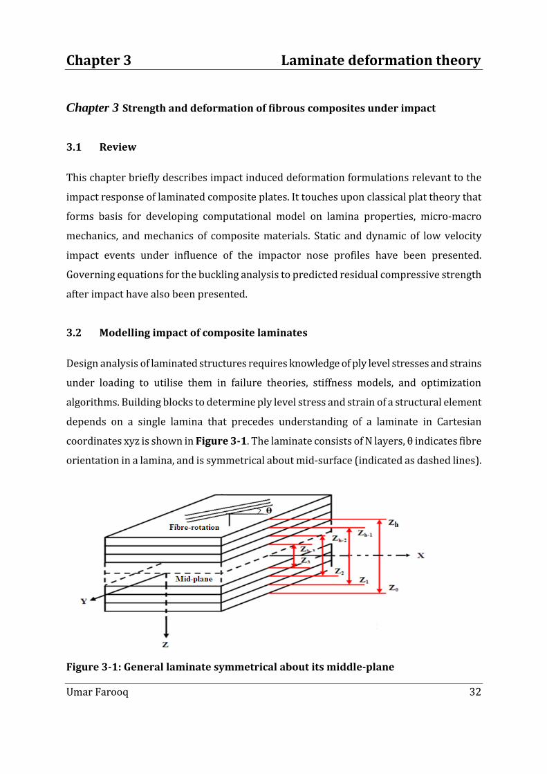
Chapter 3 Laminate deformation theory
Umar Farooq 32
Chapter 3 Strength and deformation of fibrous composites under impact
3.1 Review
This chapter briefly describes impact induced deformation formulations relevant to the
impact response of laminated composite plates. It touches upon classical plat theory that
forms basis for developing computational model on lamina properties, micro-macro
mechanics, and mechanics of composite materials. Static and dynamic of low velocity
impact events under influence of the impactor nose profiles have been presented.
Governing equations for the buckling analysis to predicted residual compressive strength
after impact have also been presented.
3.2 Modelling impact of composite laminates
Design analysis of laminated structures requires knowledge of ply level stresses and strains
under loading to utilise them in failure theories, stiffness models, and optimization
algorithms. Building blocks to determine ply level stress and strain of a structural element
depends on a single lamina that precedes understanding of a laminate in Cartesian
coordinates xyz is shown in Figure 3-1. The laminate consists of N layers, θ indicates fibre
orientation in a lamina, and is symmetrical about mid-surface (indicated as dashed lines).
Figure 3-1: General laminate symmetrical about its middle-plane
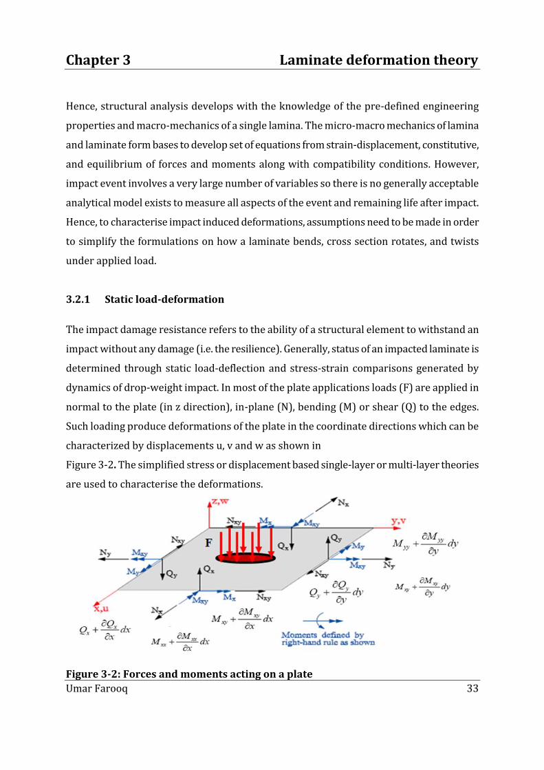
Chapter 3 Laminate deformation theory
Umar Farooq 33
Hence, structural analysis develops with the knowledge of the pre-defined engineering
properties and macro-mechanics of a single lamina. The micro-macro mechanics of lamina
and laminate form bases to develop set of equations from strain-displacement, constitutive,
and equilibrium of forces and moments along with compatibility conditions. However,
impact event involves a very large number of variables so there is no generally acceptable
analytical model exists to measure all aspects of the event and remaining life after impact.
Hence, to characterise impact induced deformations, assumptions need to be made in order
to simplify the formulations on how a laminate bends, cross section rotates, and twists
under applied load.
3.2.1 Static load-deformation
The impact damage resistance refers to the ability of a structural element to withstand an
impact without any damage (i.e. the resilience). Generally, status of an impacted laminate is
determined through static load-deflection and stress-strain comparisons generated by
dynamics of drop-weight impact. In most of the plate applications loads (F) are applied in
normal to the plate (in z direction), in-plane (N), bending (M) or shear (Q) to the edges.
Such loading produce deformations of the plate in the coordinate directions which can be
characterized by displacements u, v and w as shown in
Figure 3-2. The simplified stress or displacement based single-layer or multi-layer theories
are used to characterise the deformations.
Figure 3-2: Forces and moments acting on a plate
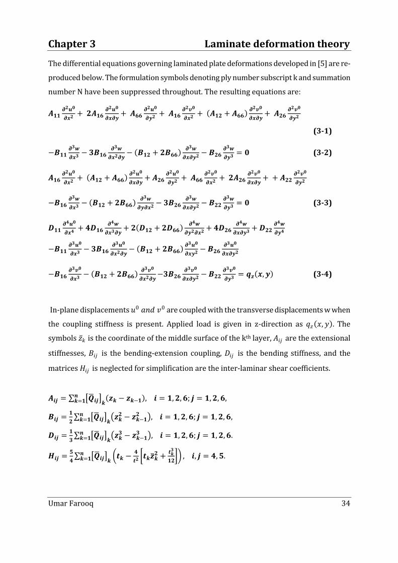
Chapter 3 Laminate deformation theory
Umar Farooq 34
The differential equations governing laminated plate deformations developed in [5] are re-
produced below. The formulation symbols denoting ply number subscript k and summation
number N have been suppressed throughout. The resulting equations are:
𝑨𝟏𝟏𝝏𝟐𝒖𝟎
𝝏𝒙𝟐 + 𝟐𝑨𝟏𝟔𝝏𝟐𝒖𝟎
𝝏𝒙𝝏𝒚+ 𝑨𝟔𝟔
𝝏𝟐𝒖𝟎
𝝏𝒚𝟐 + 𝑨𝟏𝟔𝝏𝟐𝒗𝟎
𝝏𝒙𝟐 + 𝑨𝟏𝟐 + 𝑨𝟔𝟔 𝝏𝟐𝒗𝟎
𝝏𝒙𝝏𝒚+ 𝑨𝟐𝟔
𝝏𝟐𝒗𝟎
𝝏𝒚𝟐
(3-1)
−𝑩𝟏𝟏𝝏𝟑𝒘
𝝏𝒙𝟑 − 𝟑𝑩𝟏𝟔𝝏𝟑𝒘
𝝏𝒙𝟐𝝏𝒚− 𝑩𝟏𝟐 + 𝟐𝑩𝟔𝟔
𝝏𝟑𝒘
𝝏𝒙𝝏𝒚𝟐 − 𝑩𝟐𝟔𝝏𝟑𝒘
𝝏𝒚𝟑 = 𝟎 (3-2)
𝑨𝟏𝟔𝝏𝟐𝒖𝟎
𝝏𝒙𝟐+ 𝑨𝟏𝟐 + 𝑨𝟔𝟔
𝝏𝟐𝒖𝟎
𝝏𝒙𝝏𝒚+ 𝑨𝟐𝟔
𝝏𝟐𝒖𝟎
𝝏𝒚𝟐+ 𝑨𝟔𝟔
𝝏𝟐𝒗𝟎
𝝏𝒙𝟐+ 𝟐𝑨𝟐𝟔
𝝏𝟐𝒗𝟎
𝝏𝒙𝝏𝒚+ + 𝑨𝟐𝟐
𝝏𝟐𝒗𝟎
𝝏𝒚𝟐
−𝑩𝟏𝟔𝝏𝟑𝒘
𝝏𝒙𝟑− 𝑩𝟏𝟐 + 𝟐𝑩𝟔𝟔
𝝏𝟑𝒘
𝝏𝒚𝝏𝒙𝟐− 𝟑𝑩𝟐𝟔
𝝏𝟑𝒘
𝝏𝒙𝝏𝒚𝟐− 𝑩𝟐𝟐
𝝏𝟑𝒘
𝝏𝒚𝟑= 𝟎 (3-3)
𝑫𝟏𝟏𝝏𝟒𝒖𝟎
𝝏𝒙𝟒 + 𝟒𝑫𝟏𝟔𝝏𝟒𝒘
𝝏𝒙𝟑𝝏𝒚+ 𝟐 𝑫𝟏𝟐 + 𝟐𝑫𝟔𝟔
𝝏𝟒𝒘
𝝏𝒚𝟐𝝏𝒙𝟐 + 𝟒𝑫𝟐𝟔𝝏𝟒𝒘
𝝏𝒙𝝏𝒚𝟑 + 𝑫𝟐𝟐𝝏𝟒𝒘
𝝏𝒚𝟒
−𝑩𝟏𝟏𝝏𝟑𝒖𝟎
𝝏𝒙𝟑 − 𝟑𝑩𝟏𝟔𝝏𝟑𝒖𝟎
𝝏𝒙𝟐𝝏𝒚− 𝑩𝟏𝟐 + 𝟐𝑩𝟔𝟔
𝝏𝟑𝒖𝟎
𝝏𝒙𝒚𝟐 − 𝑩𝟐𝟔𝝏𝟑𝒖𝟎
𝝏𝒙𝝏𝒚𝟐
−𝑩𝟏𝟔𝝏𝟑𝒗𝟎
𝝏𝒙𝟑 − 𝑩𝟏𝟐 + 𝟐𝑩𝟔𝟔 𝝏𝟑𝒗𝟎
𝝏𝒙𝟐𝝏𝒚−𝟑𝑩𝟐𝟔
𝝏𝟑𝒗𝟎
𝝏𝒙𝝏𝒚𝟐 − 𝑩𝟐𝟐𝝏𝟑𝒗𝟎
𝝏𝒚𝟑 = 𝒒𝒛 𝒙, 𝒚 (3-4)
In-plane displacements 𝑢0 𝑎𝑛𝑑 𝑣0 are coupled with the transverse displacements w when
the coupling stiffness is present. Applied load is given in z-direction as 𝑞𝑧 𝑥, 𝑦 . The
symbols 𝑧 𝑘 is the coordinate of the middle surface of the kth layer, 𝐴𝑖𝑗 are the extensional
stiffnesses, 𝐵𝑖𝑗 is the bending-extension coupling, 𝐷𝑖𝑗 is the bending stiffness, and the
matrices 𝐻𝑖𝑗 is neglected for simplification are the inter-laminar shear coefficients.
𝑨𝒊𝒋 = 𝑸 𝒊𝒋 𝒌 𝒛𝒌 − 𝒛𝒌−𝟏 , 𝒊 = 𝟏, 𝟐, 𝟔; 𝒋 = 𝟏, 𝟐, 𝟔,𝒏
𝒌=𝟏
𝑩𝒊𝒋 =𝟏
𝟐 𝑸 𝒊𝒋 𝒌
𝒛𝒌𝟐 − 𝒛𝒌−𝟏
𝟐 , 𝒊 = 𝟏, 𝟐, 𝟔; 𝒋 = 𝟏, 𝟐, 𝟔,𝒏𝒌=𝟏
𝑫𝒊𝒋 =𝟏
𝟑 𝑸 𝒊𝒋 𝒌
𝒛𝒌𝟑 − 𝒛𝒌−𝟏
𝟑 , 𝒊 = 𝟏, 𝟐, 𝟔; 𝒋 = 𝟏, 𝟐, 𝟔.𝒏𝒌=𝟏
𝑯𝒊𝒋 =𝟓
𝟒 𝑸 𝒊𝒋 𝒌
𝒕𝒌 −𝟒
𝒕𝟐 𝒕𝒌𝒛 𝒌
𝟐 +𝒕𝒌𝟑
𝟏𝟐 , 𝒊, 𝒋 = 𝟒, 𝟓.𝒏
𝒌=𝟏

Chapter 3 Laminate deformation theory
Umar Farooq 35
Where: Nxx, Nyy are normal force per unit length and Nxy is shear force per unit length Mxx,
Myy are bending moments per unit length and Mxy is twisting moments per unit
length,𝑉𝑥𝑎𝑛𝑑 𝑉𝑦 are components of shear force.
𝑵𝒙𝒙
𝑵𝒚𝒚
𝑵𝒙𝒚
𝒌
= 𝑨𝟏𝟏 𝑨𝟏𝟐 𝑨𝟏𝟔
𝑨𝟏𝟐 𝑨𝟐𝟐 𝑨𝟐𝟔
𝑨𝟏𝟔 𝑨𝟐𝟔 𝑨𝟔𝟔
𝒌
𝜺𝒙𝒙𝟎
𝜺𝒚𝒚𝟎
𝜸𝒙𝒚𝟎
𝒌
+ 𝑩𝟏𝟏 𝑩𝟏𝟐 𝑩𝟏𝟔
𝑩𝟏𝟐 𝑩𝟐𝟐 𝑩𝟐𝟔
𝑩𝟏𝟔 𝑩𝟐𝟔 𝑩𝟔𝟔
𝒌
(3-5)
𝑴𝒙𝒙
𝑴𝒚𝒚
𝑴𝒙𝒚
𝒌
= 𝑩𝟏𝟏 𝑩𝟏𝟐 𝑩𝟏𝟔
𝑩𝟏𝟐 𝑩𝟐𝟐 𝑩𝟐𝟔
𝑩𝟏𝟔 𝑩𝟐𝟔 𝑩𝟔𝟔
𝒌
𝜺𝒙𝒙𝟎
𝜺𝒚𝒚𝟎
𝜸𝒙𝒚𝟎
𝒌
+ 𝑫 𝑫𝟏𝟐 𝑫𝟏𝟔
𝑫𝟏𝟐 𝑫𝟐𝟐 𝑫𝟐𝟔
𝑫𝟏𝟔 𝑫𝟐𝟔 𝑫𝟔𝟔
𝒌
𝒌𝒙𝒙
𝒌𝒚𝒚
𝒌𝒙𝒚
𝒌
(3-6)
𝑽𝒚
𝑽𝒙 𝒌
= 𝑯𝟒𝟒 𝑯𝟒𝟓
𝑯𝟒𝟓 𝑯𝟓𝟓 𝒌
𝜸𝒚𝒛
𝜸𝒙𝒛 𝒌
(3-7)
Where: 𝑘𝑥𝑥 , 𝑘𝑦𝑦 , and 𝑘𝑥𝑦 are curvatures and 휀𝑥𝑥0 , 휀𝑦𝑦
0 and 𝛾𝑥𝑦0 are components of strain with
respect to the mid-surface. The Qij are the components of the lamina stiffness matrix, which
are related to the compliance and the engineering constants:
𝑸𝟏𝟏 =𝑺𝟐𝟐
𝑺𝟏𝟏𝑺𝟐𝟐−𝑺𝟏𝟐𝟐 =
𝑬𝟏𝟏
𝟏−𝝊𝟏𝟐𝝊𝟐𝟏
𝑸𝟏𝟐 = −𝑺𝟏𝟐
𝑺𝟏𝟏𝑺𝟐𝟐−𝑺𝟏𝟐𝟐 =
𝝊𝟏𝟐𝑬𝟐𝟐
𝟏−𝝊𝟏𝟐𝝊𝟐𝟏= 𝑸𝟐𝟏
𝑸𝟐𝟐 =𝑺𝟏𝟏
𝑺𝟏𝟏𝑺𝟐𝟐−𝑺𝟏𝟐𝟐 =
𝑬𝟐
𝟏−𝝊𝟏𝟐𝝊𝟐𝟏
𝑸𝟔𝟔 =𝟏
𝑺𝟔𝟔= 𝑮𝟏𝟐 (3-8)
Where the compliance coefficients are:
𝑺𝟏𝟏 = 𝟏
𝑬𝟏, 𝑺𝟐𝟐 =
𝟏
𝑬𝟐𝟐, 𝑺𝟏𝟐 = 𝑺𝟐𝟏 =
−𝝊𝟐𝟏
𝑬𝟐𝟐=
−𝝊𝟏𝟐
𝑬𝟏𝟏, 𝑺𝟔𝟔 =
𝟏
𝑮𝟏𝟐.
The Reuter transforms [R] for the strains can be performed in the same manner using
tensor strain as engineering shear strain is not a tensor quantity which is twice the tensor
shear strain, i.e., 𝛾12 = 2휀12 .
𝑹 = 𝟏 𝟎 𝟎𝟎 𝟏 𝟎𝟎 𝟎 𝟐
(3-9)

Chapter 3 Laminate deformation theory
Umar Farooq 36
The transformed reduced matrix 𝑸 is obtained from the local (1, 2) and global (x, y)
coordinate rotations at kth angles (θ) Figure 3-3 relationship matrix [T]:
𝑻 = 𝒄𝒐𝒔𝜽 𝒔𝒊𝒏𝜽−𝒔𝒊𝒏𝜽 𝒄𝒐𝒔𝜽
(3-10)
Figure 3-3: Local and global axes of matrix and rotated fibres
𝑸 = 𝑻 −𝟏 𝑸 𝑹 𝑻 𝑹 −𝟏 (3-11)
3.2.2 Impact dynamic analysis
Most of the studies on low velocity impact event are carried out as static load-deflection.
However, impact is a dynamic event in nature and internal manifestation of ply orientation
has significant effect on damage and failure modes. The reliable predictions of ply-by-ply
through-thickness stresses dynamic studies are required. The equation of motion for
laminated plate can be derived by modifying the static equilibrium equations. The Newton’s
second law can be applied to derive the dynamic equations for laminated composites. The
resulting equations for moment resultants, and transverse shear stress resultants for an
infinitesimal element were developed [5] as:

Chapter 3 Laminate deformation theory
Umar Farooq 37
𝑨𝟏𝟏
𝝏𝟐𝒖𝟎
𝝏𝒙𝟐+ 𝟐𝑨𝟏𝟔
𝝏𝟐𝒖𝟎
𝝏𝒙𝝏𝒚+ 𝑨𝟔𝟔
𝝏𝟐𝒖𝟎
𝝏𝒚𝟐+ 𝑨𝟏𝟔
𝝏𝟐𝒗𝟎
𝝏𝒙𝟐+ 𝑨𝟏𝟐 + 𝑨𝟔𝟔
𝝏𝟐𝒗𝟎
𝝏𝒙𝝏𝒚+ 𝑨𝟐𝟔
𝝏𝟐𝒗𝟎
𝝏𝒚𝟐
−𝑩𝟏𝟏𝝏𝟑𝒘
𝝏𝒙𝟑− 𝟑𝑩𝟏𝟔
𝝏𝟑𝒘
𝝏𝒙𝟐𝝏𝒚− 𝑩𝟏𝟐 + 𝟐𝑩𝟔𝟔
𝝏𝟑𝒘
𝝏𝒙𝝏𝒚𝟐− 𝑩𝟐𝟔
𝝏𝟑𝒘
𝝏𝒚𝟑= 𝝆𝟎
𝝏𝟐𝒖𝟎
𝝏𝒕𝟐 (3-12)
𝑨𝟏𝟔
𝝏𝟐𝒖𝟎
𝝏𝒙𝟐+ 𝑨𝟏𝟐 + 𝑨𝟔𝟔
𝝏𝟐𝒖𝟎
𝝏𝒙𝝏𝒚+ 𝑨𝟐𝟔
𝝏𝟐𝒖𝟎
𝝏𝒚𝟐+ 𝑨𝟔𝟔
𝝏𝟐𝒗𝟎
𝝏𝒙𝟐+ 𝟐𝑨𝟐𝟔
𝝏𝟐𝒗𝟎
𝝏𝒙𝝏𝒚+ + 𝑨𝟐𝟐
𝝏𝟐𝒗𝟎
𝝏𝒚𝟐
−𝑩𝟏𝟔𝝏𝟑𝒘
𝝏𝒙𝟑 − 𝑩𝟏𝟐 + 𝟐𝑩𝟔𝟔 𝝏𝟑𝒘
𝝏𝒚𝝏𝒙𝟐 − 𝟑𝑩𝟐𝟔𝝏𝟑𝒘
𝝏𝒙𝝏𝒚𝟐 − 𝑩𝟐𝟐𝝏𝟑𝒘
𝝏𝒚𝟑 = 𝝆𝟎𝝏𝟐𝒗𝟎
𝝏𝒕𝟐 (3-13)
𝑫𝟏𝟏
𝝏𝟒𝒖𝟎
𝝏𝒙𝟒+ 𝟒𝑫𝟏𝟔
𝝏𝟒𝒘
𝝏𝒙𝟑𝝏𝒚+ 𝟐 𝑫𝟏𝟐 + 𝟐𝑫𝟔𝟔
𝝏𝟒𝒘
𝝏𝒚𝟐𝝏𝒙𝟐+ 𝟒𝑫𝟐𝟔
𝝏𝟒𝒘
𝝏𝒙𝝏𝒚𝟑+ 𝑫𝟐𝟐
𝝏𝟒𝒘
𝝏𝒚𝟒
−𝑩𝟏𝟏
𝝏𝟑𝒖𝟎
𝝏𝒙𝟑− 𝟑𝑩𝟏𝟔
𝝏𝟑𝒖𝟎
𝝏𝒙𝟐𝝏𝒚− 𝑩𝟏𝟐 + 𝟐𝑩𝟔𝟔
𝝏𝟑𝒖𝟎
𝝏𝒙𝒚𝟐− 𝑩𝟐𝟔
𝝏𝟑𝒖𝟎
𝝏𝒙𝝏𝒚𝟐
−𝑩𝟏𝟔
𝝏𝟑𝒗𝟎
𝝏𝒙𝟑− 𝑩𝟏𝟐 + 𝟐𝑩𝟔𝟔
𝝏𝟑𝒗𝟎
𝝏𝒙𝟐𝝏𝒚−𝟑𝑩𝟐𝟔
𝝏𝟑𝒗𝟎
𝝏𝒙𝝏𝒚𝟐− 𝑩𝟐𝟐
𝝏𝟑𝒗𝟎
𝝏𝒚𝟑+ 𝝆𝟎
𝝏𝟐𝒘
𝝏𝒕𝟐= 𝒒𝒛 𝒙, 𝒚
(3-14)
In the dynamic case the in-plane displacements are coupled with the transverse
displacements w and the matrix [B] is present.
3.3 Influence of impactor’s nose shape and loading area
In order to characterise composites during impact, the theory consists of treating the
laminate like a beam in bending [5] clamped along two sides only. This theory is different
from a more classic approach in which the plate is constrained on all sides. Newton’s
second law is used to obtain acceleration. The velocity is assumed to have a nonzero value
and displacement prior to impact is zero. The acceleration equation is integrated to
expressions for instantaneous velocity and position. The acceleration works as long as the
plate is not punctured. Once the previous quantities are known, it is possible to solve for
the energy as a function of time. Formulations for calculations of impact loads according to
impactors’ shapes were developed utilising stretching (Us) and bending energy (Ub)
formulations as:

Chapter 3 Laminate deformation theory
Umar Farooq 38
𝑼𝒔 + 𝑼𝑩 𝟐𝝅
𝟎
𝒂
𝟎
= 𝑰 𝒅𝟐𝒘
𝒅𝒓𝟐 𝟐
+ 𝟏
𝒓𝟐
𝒅𝒘
𝒅𝐫 𝟐
+ 𝑱 𝟏
𝒓
𝒅𝟐𝒘
𝒅𝒓𝟐
𝒅𝒘
𝒅𝒓 + 𝑳
𝒅𝒘
𝒅𝒓 𝟒
𝒂
𝟎
𝒓𝒅𝒓
(3-15)
Where
𝑰 =𝝅
𝟖 𝟑𝑫𝟏𝟏 + 𝟑𝑫𝟐𝟐 + 𝟐𝑫𝟏𝟐 + 𝟒𝑫𝟔𝟔 ,
𝑱 =𝝅
𝟒 𝑫𝟏𝟏 + 𝑫𝟐𝟐 + 𝟔𝑫𝟏𝟐 + 𝟐𝑫𝟔𝟔 ,
𝑳 =𝝅
𝟖 𝟑𝑨𝟏𝟏 + 𝟑𝑨𝟐𝟐 + 𝟐𝑨𝟏𝟐 + 𝟒𝑨𝟔𝟔 .
Total external energy (work) W = F w0; where F = point load at the centre of circular plate
centre w0 = displacement at plate radius r = 0. Assumed displacement shape function for
boundary conditions are:
𝒘 = 𝒘𝟎 𝟏 −𝒓𝟐
𝒂𝟐 + 𝟐𝒓𝟐
𝒂𝟐 𝒍𝒐𝒈𝒓
𝒂 ,
𝒘′ = 𝒘𝟎 𝟒𝒓
𝒂𝟐 𝒍𝒐𝒈𝒓
𝒂 ,
𝒘′′ = 𝒘𝟎 𝟒
𝒂𝟐 𝒍𝐨𝒈𝒓
𝒂+
𝟒
𝒂𝟐 (3-16)
Equating the total internal energy to the external energy (equilibrium state UT – W = 0)
𝑼𝑻 = 𝑰 𝒅𝟐𝒘
𝒅𝒓𝟐 𝟐
+ 𝟏
𝒓𝟐
𝒅𝒘
𝒅𝒓 𝟐
+ 𝑱 𝟏
𝒓
𝒅𝟐𝒘
𝒅𝒓𝟐
𝒅𝒘
𝒅𝒓 + 𝑳
𝒅𝒘
𝒅𝒓 𝟒
𝒂
𝟎𝒓𝒅𝒓 = 𝑭𝒘 𝟎 = 𝟎 (3-17)
Introducing the principle of virtual displacement to the total energy, the total energy and
the work are expressed as:
𝑼𝑻 = 𝟐𝑰 𝒘′′ 𝒘′′ +𝟏
𝒓𝟐 𝒘′𝒘′ +𝑱
𝒓 𝒘′𝒘′ + 𝒘′𝒘′′ + 𝟒𝑳𝒘′ 𝟑𝒘′ 𝒓𝒅𝒓
𝒂
𝟎
= 𝑰𝟏𝟔
𝒂𝟐𝒘𝟎 + 𝑳
𝟐𝟓𝟔
𝟖𝟏𝒂𝟐𝒘𝟎
𝟑 (3-18)
𝑊 = 𝐹𝑤 0 Where 𝑤 0 is virtual displacement at r = 0.
General displacement equations for clamped circular composite plate
𝑼𝑻 = 𝑾 → 𝑰𝟏𝟔
𝒂𝟐𝒘𝟎 + 𝑳
𝟐𝟓𝟔
𝟖𝟏𝒂𝟐𝒘𝟎
𝟑 𝒘 𝟎 = 𝑭𝒘 𝟎
Where:

Chapter 3 Laminate deformation theory
Umar Farooq 39
𝑭 = 𝑰𝟏𝟔
𝒂𝟐 𝒘𝟎 + 𝑳𝟐𝟓𝟔
𝟖𝟏𝒂𝟐 𝒘𝟎𝟑 (3-19)
The strain energy found from the principle of virtual displacement. When line load is
considered one of the coordinate either (x = x0) or (y = y0) while point load is applied at the
centre, both of the coordinates are at origin and Impulse/Dirac Delta δ function its integral
is utilized for step functions. The line-load one of the dimensions is essentially zero in the
patch integral:
𝑭 𝒙𝟎, 𝒚𝟎 = 𝑭𝜹 𝒙 − 𝒙𝟎 𝜹 𝒚 − 𝒚𝟎 (3-20)
The rectangular patch load the function is:
𝑭 𝒙, 𝒚 = 𝑭𝜹 𝒙 − 𝒙𝟎 𝒙𝟎+𝜶
𝒙𝟎−𝜶𝒅𝒙 𝑭𝜹 𝒚 − 𝒚𝟎
𝒙𝟎+𝜷
𝒙𝟎−𝜷𝒅𝒚 (3-21)
The circular patch load Eq. (3-20) may be transform as
𝑭 𝒓, 𝜽 = 𝑭𝜹 𝒓 − 𝒓𝟎 𝒓𝟎=𝒓
𝒓𝟎=𝟎𝒅𝒓 𝑭𝜹 𝜽 − 𝜽𝟎
𝟐𝝅
𝜽𝟎=𝟎𝒓𝒅𝒓𝒅𝜽 (3-22)
In case of a point load is to be considered the coordinates become (r = r0) and (θ = θ0).
3.4 Residual strength from buckling analysis
Residual strength is also called damage tolerance since it refers to the prediction of residual
mechanical properties of the damaged structure through buckling analysis. When a flat
plate is subjected to low in-plane compressive loads, it remains flat and is in equilibrium
condition. As the magnitude of the in-plane compressive load increases, however, the
equilibrium configuration of the plate is eventually changed to a non-flat configuration and
the plate becomes unstable. The magnitude of the compressive load at which the plate
becomes unstable is called the critical buckling load. The buckling of a plate involves two
planes and two boundary conditions on each edge of the plate. In order to develop the
equation to predict buckling under in-plane loads the coupling was considered. Assuming
the differential element rotated in an out of plane position as shown in Figure 3-4 [5].

Chapter 3 Laminate deformation theory
Umar Farooq 40
Figure 3-4: Differential element positions for buckling analysis
The coupling between the in-plane forces Nxx, Nyy and Nxy and the out of plane deflections,
w, can be used to develop and predict buckling under in-plane loading moment resultants,
and transverse shear stress resultants for an infinitesimal element were developed [5]
coupling moment resultants, and transverse shear stress resultants for an infinitesimal
element as:
𝑫𝟏𝟏
𝝏𝟒𝒘
𝝏𝒙𝟒+ 𝟒𝑫𝟏𝟔
𝝏𝟒𝒘
𝝏𝒙𝟑𝝏𝒚+ 𝟐 𝑫𝟏𝟐 + 𝟐𝑫𝟔𝟔
𝝏𝟒𝒘
𝝏𝒚𝟐𝝏𝒙𝟐+ 𝟒𝑫𝟐𝟔
𝝏𝟒𝒘
𝝏𝒙𝝏𝒚𝟑+ 𝑫𝟐𝟐
𝝏𝟒𝒘
𝝏𝒚𝟒
−𝑩𝟏𝟏
𝝏𝟑𝒖𝟎
𝝏𝒙𝟑− 𝟑𝑩𝟏𝟔
𝝏𝟑𝒖𝟎
𝝏𝒙𝟐𝝏𝒚− 𝑩𝟏𝟐 + 𝟐𝑩𝟔𝟔
𝝏𝟑𝒖𝟎
𝝏𝒙𝒚𝟐− 𝑩𝟐𝟔
𝝏𝟑𝒖𝟎
𝝏𝒙𝝏𝒚𝟐− 𝑩𝟏𝟔
𝝏𝟑𝒗𝟎
𝝏𝒙𝟑
− 𝑩𝟏𝟐 + 𝟐𝑩𝟔𝟔 𝝏𝟑𝒗𝟎
𝝏𝒙𝟐𝝏𝒚−𝟑𝑩𝟐𝟔
𝝏𝟑𝒗𝟎
𝝏𝒙𝝏𝒚𝟐 − 𝑩𝟐𝟐𝝏𝟑𝒗𝟎
𝝏𝒚𝟑
= 𝒒 𝒙, 𝒚 + 𝑵𝒙𝒙𝝏𝟐𝒘
𝝏𝒙𝟐 + 𝟐𝑵𝒙𝒚𝝏𝟐𝒘
𝝏𝒙𝝏𝒚+ 𝑵𝒚𝒚
𝝏𝟐𝒘
𝝏𝒚𝟐 (3-23)
The Eq. (3-22) consists of additional terms due to the in-plane forces. Due to the presence
of the bending-twisting coupling terms (D16 and D26) there is no exact solution of the

Chapter 3 Laminate deformation theory
Umar Farooq 41
buckling equations for plates of finite dimensions. The existence of even small bending-
twisting coupling terms (e.g. an angle-ply plate with a large odd number of alternating
plies) could provide considerably different results than those obtained with zero D16 and
D26 terms.
3.5 Selection of finite element simulation methodology
The experimental methods are resource consuming, data integrity is difficult to maintain,
and less competitive in today’s market economy. While analytical techniques can only be
applied to limited and simplified problems. Numerical simulations could be obtained by
transformation of the mathematical formulations, applying differencing schemes, and
writing codes. However, the approach needs extensive efforts and time. But literature
search has shown the efficient way to obtain solutions of variety of engineering problems
using finite element based software. Computer codes previously developed have evolved
and emerged into a great deal of standard public domain software for solving physical
problems effectively to an acceptable level of accuracy. Such software are being utilised for
solving physical problems effectively to an acceptable level of accuracy due to their built-in
features. The features can be employed and modified for specific analyses with minimum
efforts such as impact on composite laminates. Use of the standard software is preferred
due to their built-in features. The features can be employed and modified for specific
analyses with minimum efforts such as impact on composite laminates. The software PTC
SimulateTM and ABAQUSTM were chosen to perform simulations for particular part of the
investigation because of their ease with the initial modelling. The software incorporates a
variety of linear and nonlinear shell elements that could accommodate stacks of hundred or
more plies. The simulation analyses could be extended by scaling structural components.
Therefore, the software was chosen for the current investigation and industry provided
input data given in [1] was utilised. Common simulation process is shown in Figure 3-5.

Chapter 3 Laminate deformation theory
Umar Farooq 42
Figure 3-5: Common finite element simulation process of engineering problems.
3.6 Summary
This chapter incorporated the relevant theoretical work used to approximate the damage
resistance and damage tolerance capabilities of the impacted composite laminates under
various impactor nose profiles. Selection of finite element simulations as a solution method
has also been outlined.

Chapter 4 Load-deflection simulation
Umar Farooq 43
Chapter 4 Load-deflection simulation using PTC Creo SimulateTM software
4.1 Review
This chapter describes simulation produced results of carbon fibre reinforced composite
laminates subjected to point, low, medium and large nose impactors to predict damage
existence, location, type, and size. Static load-deflection methodology was implemented in
PTC Creo SimulateTM software. Simulation cases of eight, sixteen, and twenty-four ply
laminates were investigated. Validations of the selected experimental and simulated results
were carried out. Comparisons and discussions of results produced from simulation of
laminates embedded with ply-by-ply pre-assumed damage zones corresponding to four
impactor nose profiles from symmetric and un-symmetric lay-ups and variations in loading
areas under impactor nose are also presented.
4.2 Laminates, impactor nose profiles, and material properties
4.2.1 Laminates and impactors
Geometrical properties were proposed in [1], the laminates of code IM7/8552 and
dimensions: 150 mm x 120 mm x 2.88 mm were selected. Fibre orientations are shown in
Figure 4-1 (a) and laminate is shown in Figure 4-1(b). Impact behaviour of laminates
investigated for:
a) 8-Ply laminates consisted of lay-ups code [45/0/-45/90]S
b) 16-Ply laminates of code [45/0/-45/90]2S, and
c) 24-Ply laminates of code [45/0/-45/90]3S.
Testing area consisting of circular cut-outs of 100 (mm) diameter is shown in Figure
4-1(c).
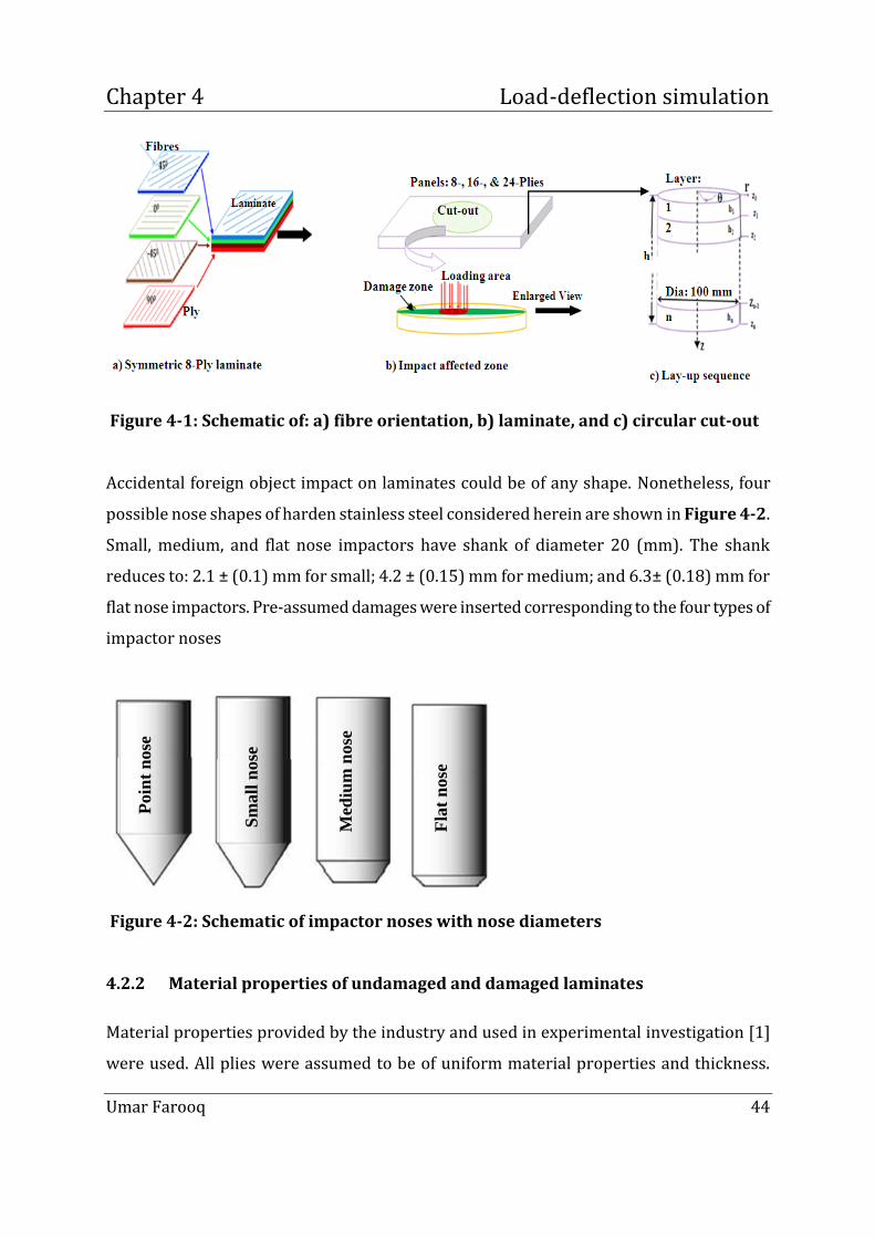
Chapter 4 Load-deflection simulation
Umar Farooq 44
Figure 4-1: Schematic of: a) fibre orientation, b) laminate, and c) circular cut-out
Accidental foreign object impact on laminates could be of any shape. Nonetheless, four
possible nose shapes of harden stainless steel considered herein are shown in Figure 4-2.
Small, medium, and flat nose impactors have shank of diameter 20 (mm). The shank
reduces to: 2.1 ± (0.1) mm for small; 4.2 ± (0.15) mm for medium; and 6.3± (0.18) mm for
flat nose impactors. Pre-assumed damages were inserted corresponding to the four types of
impactor noses
Figure 4-2: Schematic of impactor noses with nose diameters
4.2.2 Material properties of undamaged and damaged laminates
Material properties provided by the industry and used in experimental investigation [1]
were used. All plies were assumed to be of uniform material properties and thickness.
P
oin
t n
ose
S
mall
nose
M
ediu
m n
ose
F
lat
nose

Chapter 4 Load-deflection simulation
Umar Farooq 45
Material properties, effective material properties and degraded material properties are
shown in Table 4-1.
Table 4-1: Properties of laminate and impactor [1]
Property IM7/8552
( 0o )
IM7/8552
( 90o )
IM7/8552
(45/0/-45/90)
Condition RT Dry RT Dry RT Dry
Tensile Modulus GPa 150 15 65
Compression Modulus GPa - - 55
In-plane Shear Modulus GPa 5.7*
-
5.7
Flexural Modulus GPa - - 48
Tensile Strength MPa 1350 20 870
Compressive Strength MPa - - 630
Ultimate In-plane Shear
Strength
MPa 121 121 120
Inter-laminar Shear Strength MPa - - 53
Flexural Strength MPa - - 1170
Ultimate Tensile Strain % 0.9 0.2 1.35
Ultimate Compressive Strain % - - 1.22
Ultimate In-plane Shear Strain % - - -
Tensile Poisson’s Ratio 0.33 0.02 0.33 *determined using +/- 45o tensile tests
The degraded materials shown in Table 4-2 and the applied load were proposed in [1].
There are various material degradation rules to reduce material properties (matrix or
fibre) of the embedded damage zones. Coefficients of the stiffness matrices are required to
reduce to zero for tensile and compressive failure modes. However, in order to avoid
numerical problems, the stiffness matrix is equated to a very small number [154] and
[155]. Majority of material degraded practice are described as:
a) If matrix failure is assumed then the material loses its traverse properties and
Poisson’s ratio effect.
b) If the failure mode is fibre-matrix shearing mode, then the material loses its shear
properties and the Poisson’s effect. But elastic constants do not reduce.

Chapter 4 Load-deflection simulation
Umar Farooq 46
c) If delamination causes the failure, then the material loses its properties in the
thickness direction, Poisson’s effect and laminate will not be able to carry shear
loads. But elastic constants in fibre and lateral directions are assumed intact.
d) For the matrix and fibre failure, elastic constant in lateral direction and major
Poisson’s ratios are reduced to zero. However, elastic constant in fibre direction is
not reduced, considering the matrix failure, the shear constants are reduced for
fibre failure calculated from an expression of exponential decay [154].
In cases of inserting hole, soft inclusion, artificial damage zones, and softening stiffness
authors reduced engineering according to requirements of the problems. Material
degradation parameters used to reduce elastic and shear constants in [1] were selected as
shown in Table 4-2 and assigned to partitioned zones created in Table 4-3 (minus
overlapping areas).
Table 4-2: Degraded material properties for pre-assumed damage zone
Property IM7/8552
Tensile Modulus (E1) GPa 2
Tensile Modulus (E2) GPa 1
Tensile Modulus (E3) GPa 1
In-plane Shear Modulus (G12) GPa 0.5
In-plane Shear Modulus (G13) GPa 0.5
In-plane Shear Modulus (G23) GPa 0.25
Poisson’s Ratio (12) 0.33
Poisson’s Ratio (13) 0.33
4.3 Selection of methodology and software
4.3.1 The load-deflection methodology
When an impact event occurs to a structural component visual damage is not always
apparent although there can be severe underlying damage. Correlation between the static
load-deflection to visible damage size (dent or crack length) is made to approximate the
impact damage. The correlation method could effectively estimate the low velocity impact
Chapter 4 Load-deflection simulation
Umar Farooq 47
damage for: transverse force, flexural and contact events. Deflection can be directly
measured with greater accuracy and failure in tension or compression can be achieved due
to low shear strength. Hence, using the load-deflection analogy elastic failure can also be
predicted. The load-deflection methodology greatly simplifies the analysis as time-
dependent terms in the governing equations disappear and much more data can be
obtained. Moreover, damage initiation and propagation can be more easily detected and
maximum transverse force can be better controlled.
4.3.2 The commercial software PTC Creo SimulateTM
The literature search has shown the efficient way to obtain solutions of variety of
engineering problems using finite element based software. Computer codes previously
developed have evolved and emerged into a great deal of standard public domain software.
Such software are being utilised for solving physical problems effectively to an acceptable
level of accuracy due to their built-in features. The features can be employed and modified
for specific analyses with minimum efforts such as impact on composite laminates. Most of
the researchers have already used PTC Creo SimulateTM for analysis of simple laminated
composite problems. The software incorporates a variety of linear and nonlinear shell
elements that could accommodate stacks of several plies. The simulation analyses could be
extended by scaling structural components. Therefore, the software was chosen for the
current investigation.
4.4 Developing static load-deflection computational model
Fully-clamped eight, sixteen, and twenty-four plies circular laminates of diameter: 100 mm
were incorporated in PTC Creo SimulateTM software as this best represents the actual
experimental test programme samples. The laminates were meshed with sweeping
meshing techniques. Computational domains of all the test laminates were theoretically
partitioned into two areas hence two different element types were assigned to the domain.
First part not directly under the impactor nose tip was meshed by fully integrated four-
nodded general purpose linear shell elements.

Chapter 4 Load-deflection simulation
Umar Farooq 48
The central part directly under the nose tip was meshed by reduced integration total
number of triangular shell elements. Typical simulation models of 24-Ply laminate
consisting of mapped and sweeping mesh types are shown in Figure 4-3 (a), (b) & (c).
Figure 4-3: A typical pre-processed meshed model for 24-Ply laminate
The static load of 8.9 (KN) per unit area proposed in [1] was applied at the centre in vertical
direction in all cases. Moreover, the load 8.9 (KN) remained constant when applied at a
point in the centre to avoid singularity as shown in Figure 4-4 (a). The constant load was
applied in the case of point-load impactor as there was no partitioning of the loading area.
Simulations cases consist of:
a) Load applied at circular areas corresponding to the semi-minor axes of the impactor
nose profiles
b) Inserted pre-assumed damage zones were rotated (aligned in fibre direction) and
were equal to areas of relevant impactor nose profiles
c) Pre-assumed damage zones were equal to a single ply thickness in the relevant
laminate
d) The damage zones were inserted ply-by-ply across thickness of the laminates.
A pre-processed simulation generated 8-Ply laminate applied at circular areas
corresponding to impactor noses were selected. The laminates embedded with damage

Chapter 4 Load-deflection simulation
Umar Farooq 49
zones corresponding to the impactor nose profiles (semi-minor axes) are shown in Figure
4-4 (a)-(d).
Figure 4-4: Typical computer generated damage resistance models
4.5 Static load-deflection predictions of undamaged laminates
4.5.1 Approximation of damage shapes corresponding to impactor nose profiles
Static load-deflection tests of the carbon fibre/epoxy laminate were conducted by James
[1]. Gross damage areas recorded during the impact testing ranged from 500 mm2 to 8800
mm2 were found to be circular in shape [1]. Photographs of the flat nose impacted
laminates can be seen from front surface of Figure 4-5 (a) and close up image after full
penetration Figure 4-5(b) that damage shapes are circular.
a) b)
Figure 4-5: Photographs: a) front surface and b) close up image
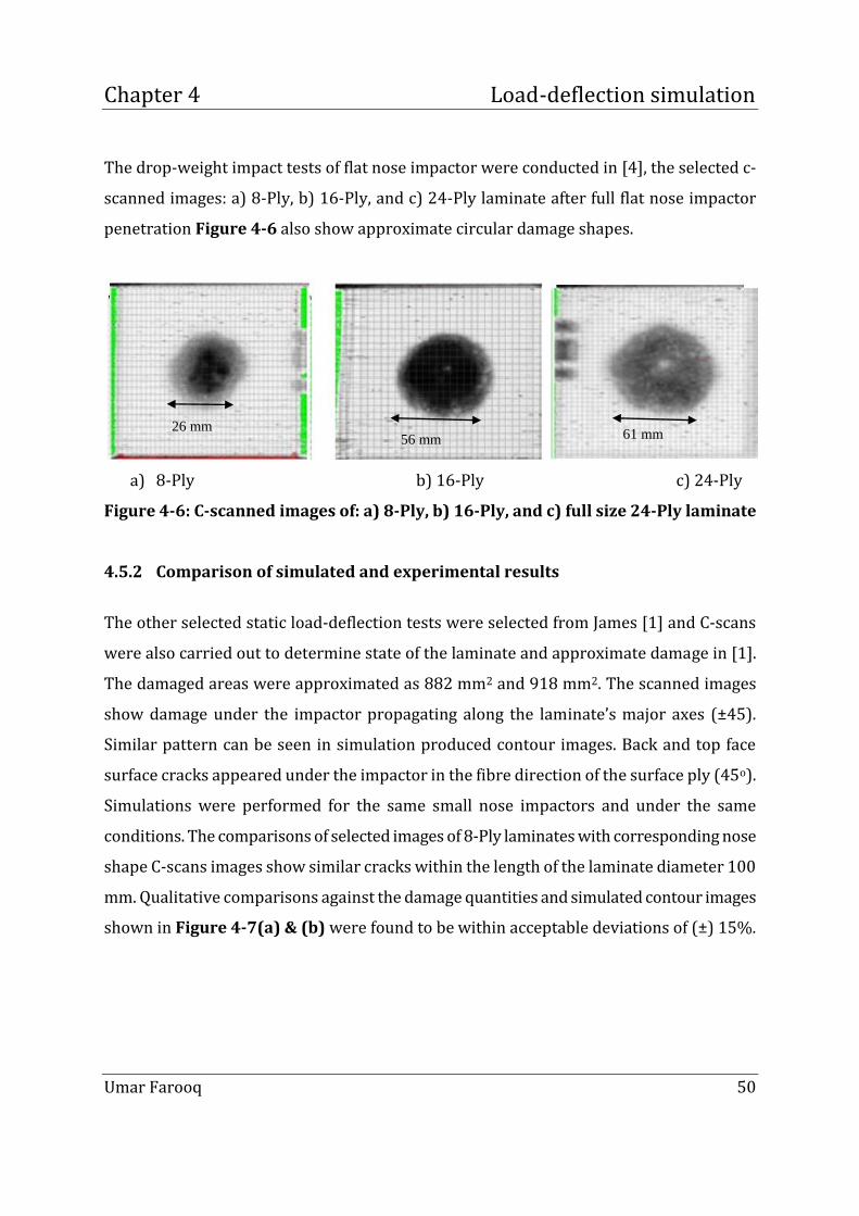
Chapter 4 Load-deflection simulation
Umar Farooq 50
The drop-weight impact tests of flat nose impactor were conducted in [4], the selected c-
scanned images: a) 8-Ply, b) 16-Ply, and c) 24-Ply laminate after full flat nose impactor
penetration Figure 4-6 also show approximate circular damage shapes.
a) 8-Ply b) 16-Ply c) 24-Ply
Figure 4-6: C-scanned images of: a) 8-Ply, b) 16-Ply, and c) full size 24-Ply laminate
4.5.2 Comparison of simulated and experimental results
The other selected static load-deflection tests were selected from James [1] and C-scans
were also carried out to determine state of the laminate and approximate damage in [1].
The damaged areas were approximated as 882 mm2 and 918 mm2. The scanned images
show damage under the impactor propagating along the laminate’s major axes (±45).
Similar pattern can be seen in simulation produced contour images. Back and top face
surface cracks appeared under the impactor in the fibre direction of the surface ply (45o).
Simulations were performed for the same small nose impactors and under the same
conditions. The comparisons of selected images of 8-Ply laminates with corresponding nose
shape C-scans images show similar cracks within the length of the laminate diameter 100
mm. Qualitative comparisons against the damage quantities and simulated contour images
shown in Figure 4-7(a) & (b) were found to be within acceptable deviations of (±) 15%.
26 mm 56 mm 61 mm

Chapter 4 Load-deflection simulation
Umar Farooq 51
Figure 4-7: Comparison of 8-Ply laminate impacted by impact nose 2.1 mm.
4.5.3 Comparison of simulated results for flat and round nose impactors
To compare with the test findings the model simulated flat and round nose impact of 8-Ply
laminates. Correponding area of the impactor nose profile can be can be seen from Figure
4-8 reported in [4]

Chapter 4 Load-deflection simulation
Umar Farooq 52
Figure 4-8: Simulated contours of 8-Ply laminates: a) flat and b) round nose.
To simplify the analysis and compare with the test findings the stress-based model was
simulated. Higher stress values can be seen in legend table while gross damage zones are
depicted at cntral zones in blue and red colors in Figure 4-9 (a) and (b). As diameters of
the laminates are 100 mm and diameter of the stresses areas under flat and round nose
impactors is 5 mm. However, it can be seen from the images that the round nose impact
created compressive (blue area) while flat nose impact crated tensile stresses (red area).
Moreover, stresses produced with flat nose impact are higher than the stresses created
with round nose impactor.
Figure 4-9: Simulated 8-Ply laminate: a) legend table and b) stress contours [4].
100 mm 100 mm
5 mm 5 mm

Chapter 4 Load-deflection simulation
Umar Farooq 53
4.5.4 Influence of loading area influence to undamaged laminates
The impact responses of the laminates were determined by correlating deflected zone in
red to the impactor’s nose tip. It can be seen from Figure 4-10(a) that the red zone
generated by the point load is small but deflection value 1.029 mm is larger. In Figure
4-10(b) deflection value 0.988 mm is also large for impactor nose 2.1 mm. The Figure
4-10(c) shows relatively medium size red zones and deflection value 0.864 mm
corresponding to medium impactors’ nose tips. Similarly, a larger red zone with small
deflection values 0.741 mm was produced by the corresponding large impactor nose
Figure 4-10(d). The anticipated behaviour of small red zone and larger deflection value by
small nose tip on the surface and large red zone by large nose tip on the surface was
anticipated. The consistent behaviour predicted from all the four type of impact responses
indicates that the simulation is reliable.
a) Point-load b) Nose 2.1 mm
c) Nose 4.2 mm d) Nose 6.3 mm
Figure 4-10: Images show damage in red colour

Chapter 4 Load-deflection simulation
Umar Farooq 54
4.5.5 Influence of partitioned loading area to undamaged laminates
Kim and Goo in [156] modelled the effects of altering the ratios between impactor nose
lengths to impactor radii (0, 1, …, 10) on the impact response of glass-fibre plates. He found
that as the ratio decreased the impactor nose becomes blunt, the peak force increased and
the impact duration decreased. To make realistic comparison of nose effects under various
loads, the loading areas were radially partitioned in uniform ten divisions. Since applied
load is constant, influence of applied loads were simulated using portions of loading areas.
Successive partitions of the circular loading areas are based on the quantities shown in
Table 4-3. Every loading area under impactors’ nose tips were portioned into ten radial
divisions for realistic simulation of variable loading conditions.
Table 4-3: Loading areas mm2
Loading areas (mm2)
Small Medium Large (Flat)
10 Partitions of each loading areas
0.03 0.14 0.31
0.14 0.55 1.25
0.31 1.25 2.81
0.55 2.22 4.99
0.87 3.47 7.85
1.25 4.99 11.23
1.70 6.79 15.35
2.22 8.87 19.96
2.81 11.23 25.35
3.47≅4 13.86≅ 14 31.19≅ 31

Chapter 4 Load-deflection simulation
Umar Farooq 55
Simulations were performed for ten radial divisions to reliably capture the localised
deflections generated from impactor nose profile against deflection value and red damage
zone. Ten uniform distributions of the loading areas under the three nose tip of impactors
for 8-, 16-, and 24-Ply laminates. Comparison of plots show higher deflections at the
beginning where loading areas were small (load gets higher) Figure 4-11, Figure 4-12, &
Figure 4-13. Consistent behaviour of the deflection values under the impactor nose
profiles can be seen for all the lay-up sequences. Difference remains negligible despite
different number of plies in lay-up sequences can be attributed to uniform thickness for all
laminates.
Figure 4-11: Deflection against radius of loading area
Figure 4-12: Deflection against radius of loading area

Chapter 4 Load-deflection simulation
Umar Farooq 56
Figure 4-13: Deflection against radius of loading area
4.5.6 Selection of the pre-assumed damage methodology
Experimental studies for damage tolerance employed soft inclusion as a pre-assumed-
damage zone of known position, size and shape in [1]. Experiments and analysis of
laminates with artificial damage are reported in [9] and [1]. The same pre-assumed damage
methodology is selected for the present investigation. These damage areas have oblong,
elliptical-peanut shape with its major axis oriented in the direction of fibres in the lower ply
at the interface. However, gross damage areas recorded during the impact testing of the
carbon fibre/epoxy laminate ranged from 500 mm2 to 8800 mm2 and were circular in
shape [1]. An 8-Ply circular symmetric laminate was selected to show accumulation of pre-
assumed damage zones equivalent to impactor nose shape in successive ply-by-ply
locations. The quantities of elliptical pre-assumed damage zones consisting of degraded
material properties corresponding to impactor nose profiles oriented in plies at 450, 00, -
450, and 900 angles are shown in Table 4-4.

Chapter 4 Load-deflection simulation
Umar Farooq 57
Table 4-4: Schematics of damaged ply and damaged areas mm2
Area of laminate:
7857 mm2
Semi-major axis: a
Semi-minor axis: b
mm
No of damage zone
100
2.1 4.2 6.3
Damage zone = π ab
mm2
None
0 0 0
1 π ab 660 1320 1980
Overlapping zone: b2 No of zone Formulation Net damage: mm2
2 2π ab -bb
1316 2622 3920
3
3π ab -2b.b
1971 3925 5861
4
4π ab -3b.b
2627 5227 7801
Pre-assumed damage under point load impactor was assumed to be 100 (mm2) in all cases
to avoid numerical singularity. Calculations for approximating the pre-assumed damage
zones corresponding to small, medium, and flat impactor nose profiles are shown in Table
4-5. Overlapping damage zones are deducted at every simulation to avoid already degraded
material properties in black damage zone again Figure 4-14.
a
b

Chapter 4 Load-deflection simulation
Umar Farooq 58
Figure 4-14: Overlapping zones a) single, b) two, and c) Three
Table 4-5: Approximation of net damage zones
Impactor nose profiles
Semi-major axis: a Semi-minor axes: b
100 (mm) Small Medium Flat
2.1 (mm) 4.2 (mm) 6.3 (mm)
Elliptical damage zone (mm2): π(a x b)
π(2.1x100): 660 π(4.2x100): 1320 π(6.3x100): 1980
Overlapping zone (mm2): b*b
(2.1x2.1): 4.41 (4.3x4.2): 17.64 (6.3x6.3): 39.69
Number of overlapping damage zone
1 2 3
Approximation of net damage zone (mm2)
2π a.b –b.b 3π ab -2b.b 4π ab -3b.b
4.6 Simulation of pre-assumed damage induced load-deflection
Experimental studies consistently report that the internal damage occurs due plies with
different orientations of laminates impacted at the top [1]. These damage areas have oblong
(elliptical-peanut) shape with its major axis oriented in the direction of fibres in the lower
ply at the interface. The damage zones consisting of degraded materials properties
corresponding to impactor nose profiles were simulated. Knowledge about the existing and
position of an impact event on a composite structure is useful preliminary information for

Chapter 4 Load-deflection simulation
Umar Farooq 59
subsequent characterisation of an eventual damage. When position of impact damage is
known with confidence, inspection of the structure can be limited to that region.
Information about location may significantly reduce complexity of the damage mode
identification and problems related to damage size. To correlate internal locations, type and
size of the impact damage simulations were carried out for equivalent pre-assumed
damage zones inserted at various through-thickness locations of laminates. The same
analogy is applied to study variation in loading area under impactors’ nose tips for stacking
sequences consisting of different number of plies. Simulations incorporated with pre-
assumed damage zones of elliptical shapes under relevant impactors’ nose sizes were
carried out. Simulations were also performed for various radial divisions to reliably capture
the localised deflections generated from impactor nose profiles against pre-assumed
internal damage zones. For efficient computations, symmetric lay-up configurations of the
laminates were considered in most of the cases. Simulations for symmetric laminates can
be obtained at relatively faster speed as they do not consider tensile-bending generated
coupling, number of identical plies placed at equal distance above and below the mid-plane
generates zero coupling matrices. Moreover, comparisons of the results for certain cases of
symmetric and un-symmetric lay-ups show negligible differences (not being reported).
However, to study effects of ply orientation, simulation of non-symmetric laminates were
also carried out. Those simulations included effects from bending-extension, bending-
twisting moments that implies curvature in addition to the in-plane deformations. Static
load-deflection simulation cases with effect of damage induced changes in indentation-
flexure models are shown in flowchart Figure 4-15.

Chapter 4 Load-deflection simulation
Umar Farooq 60
Figure 4-15: Static load-deflection analysis flowchart
4.7 Discussion of the simulation generated results
4.7.1 Impactor nose shape against lay-up sequence
Simulations were performed for the cases depicted in Figure 5-16. To study influence of
the successive ply-by-ply pre-assumed damage the 8-Ply un-symmetric laminate lay-ups
are selected for discussions. Laminates were simulated with pre-assumed successive
damage zones. Results generated by impactor nose shape 2.1 mm in Table 4-6 and
impactor nose shape of 4.2 mm in Table 4-7 and impactor nose shape 6.3 are shown in
Table 4-6. The ply-by-ply pre-assumed successive damage quantities produced similar
deflection quantities in symmetric and un-symmetric lay-ups. Moreover, consistent linear
proportional trends among damage quantities and simulated deflection values can be seen.

Chapter 4 Load-deflection simulation
Umar Farooq 61
Table 4-6: 8-Ply laminate simulated under impactor nose diameter 2.1 mm
Impactor
nose
mm
Damage zone in ply at angle
Symmetric lay-up Un-symmetric layup
450 450& 00 450,00& 900 all 450 450&00 450,00&900 all
Computed deflection mm
0.00 0.88 0.89 0.94 0.97 0.8 0.88 0.89 0.94
0.21 0.792 0.88 0.900 0.9 0.21 0.79 0.88 0.9
0.315 0.704 0.78 0.8 0.81 0.35 0.71 0.81 0.82
0.42 0.62 0.7 0.71 0.72 0.42 0.63 0.72 0.74
0.525 0.53 0.6 0.62 0.63 0.52 0.52 0.61 0.63
0.63 0.44 0.51 0.52 0.54 0.63 0.44 0.52 0.54
0.735 0.35 0.41 0.43 0.44 0.74 0.36 0.42 0.43
0.84 0.26 0.3 0.33 0.34 0.83 0.26 0.31 0.33
0.945 0.18 0.2 0.21 0.22 0.95 0.17 0.24 0.25
1.05 0.089 0.1 0.11 0.11 1.05 0.09 0.1 0.12

Chapter 4 Load-deflection simulation
Umar Farooq 62
Table 4-7: 8-Ply laminate simulated under impactor nose diameter 4.2 mm
Impactor
nose
mm
Damage zone in ply at angle
Symmetric lay-up Un-symmetric layup
450 450& 00 450,00& 900 all 450 450&00 450,00&900 all
Computed deflection mm
0.21 0.73 0.61 0.66 0.75 0.73 0.61 0.66 0.75
0.42 0.66 0.55 0.60 0.67 0.66 0.55 0.60 0.67
0.63 0.58 0.49 0.53 0.60 0.58 0.49 0.53 0.60
0.84 0.51 0.43 0.46 0.52 0.51 0.43 0.46 0.52
1.05 0.44 0.37 0.40 0.45 0.44 0.37 0.40 0.45
1.26 0.36 0.30 0.33 0.37 0.36 0.30 0.33 0.37
1.47 0.29 0.24 0.26 0.30 0.29 0.24 0.26 0.30
1.68 0.22 0.18 0.20 0.22 0.22 0.18 0.20 0.22
1.89 0.15 0.12 0.13 0.15 0.15 0.12 0.13 0.15
2.1 0.07 0.06 0.07 0.07 0.07 0.06 0.07 0.07
The ply-by-ply deflection values are compared for 8-Ply un-symmetric laminates with
successive accumulated damage plies in Table 4-8.

Chapter 4 Load-deflection simulation
Umar Farooq 63
Table 4-8: 8-Ply laminate simulated under impactor nose diameter 6.3 mm
Impactor
nose
mm
Damage zone in ply at angle
Symmetric lay-up Un-symmetric layup
450 450& 00 450,00& 900 all 450 450&00 450,00&900 all
Computed deflection mm
0.32 0.06 0.00 0.08 0.08 0.08 0.08 0.09 0.10
0.63 0.12 0.07 0.16 0.16 0.17 0.17 0.18 0.20
0.95 0.18 0.14 0.23 0.25 0.25 0.25 0.26 0.30
1.26 0.24 0.28 0.31 0.33 0.34 0.34 0.35 0.40
1.58 0.30 0.35 0.39 0.41 0.42 0.42 0.44 0.50
1.89 0.36 0.42 0.46 0.49 0.51 0.51 0.53 0.60
2.21 0.42 0.49 0.55 0.57 0.59 0.59 0.61 0.70
2.52 0.48 0.56 0.62 0.65 0.68 0.68 0.70 0.80
2.84 0.55 0.63 0.70 0.74 0.76 0.76 0.79 0.90
3.15 0.61 0.70 0.78 0.82 0.85 0.85 0.88 0.94
4.7.2 Influence of damage locations
The ply-by-ply bar charts are compared for 8-Ply un-symmetric laminates impacted at 6.3
mm nose against deflection values generated from successive pre-assumed damage plies.
The corresponding deflection values are relatively higher at the top ply locations. This
trend gets reversed as impactor damage located inside the laminate, the increase deflection
values start decreasing. This happens due to increase in loading area under impactor nose
shape. Since the results were generated by reducing load. The comparison and correlation
between impactor nose, deflection values, and location of damage zones are shown in
column charts Figure 4-16.

Chapter 4 Load-deflection simulation
Umar Farooq 64
Figure 4-16: Deflection v location of damage ply for 8-Ply at nose 6.3 mm
To further clarify the comparison of reverse trends due to damage locations plotted against
the impactor’s nose radii in Figure 4-17. It can be seen from the plot increasing impactor
nose radii generated corresponding decreasing deflection values. It also confirms that pre-
assumed damage ply deflection values increase in proportion to the damaged plies.
Figure 4-17: Deflection v loading area for 8-Ply at nose 6.3 mm

Chapter 4 Load-deflection simulation
Umar Farooq 65
4.7.3 Impactor nose on against successive damage zone and loading area
Cases of ten loading partitions corresponding to impactor of nose profiles: 2.1, 4.2, and 6.3
mm were simulated with pre-assumed damage zones. The 24-Ply laminates embedded with
successive damage zone corresponding to impactor nose profiles is selected for comparison
and discussion. The laminate with single pre-assumed damage zone, simulated image
exhibiting red zone as damage, and deflection value in column 3 are shown in Table 4-9.
Table 4-9: Top ply of 24-Ply laminate under impactor nose 6.3 mm
Cases of ten loading partitions corresponding to area under impactor tips are compared in
column charts Figure 4-18. The comparison shows larger deflection values when loading
areas were relatively smaller under all the impactor noses. Moreover, larger local deflection
values under smaller impactor nose and smaller deflection values under larger impactor
nose. Furthermore, the deflection vales show inverse proportional relation between
impactor nose and deflection values.

Chapter 4 Load-deflection simulation
Umar Farooq 66
Figure 4-18: Deflection v loading area for 24-Ply laminate 3 noses
The selected simulation results for two damage zones are shown in Table 4-10 and Figure
4-19. Similar trends can be seen, the larger deflection values when radius of the loading
area is smaller.

Chapter 4 Load-deflection simulation
Umar Farooq 67
Table 4-10: Top-ply 24-Ply laminate under impactor nose 6.3 mm
Figure 4-19: Deflection v loading area for 24-Ply laminate 3 noses
The selected results for three damage zones can be seen in Table 4-11 and Figure 4-20.
The consistent trends affirm the inverse proportionality relation between loading are and
deflection values.

Chapter 4 Load-deflection simulation
Umar Farooq 68
Table 4-11: Top-ply 24-Ply laminate under impactor nose 6.3 mm
Figure 4-20: Deflection v loading area for 24-Ply laminate 3 noses
Same trends can be seen for four pre-assumed damage zone simulations as shown in Table
4-12 and Figure 4-21 for 4 damage zones. The comparison confirmed that size of the pre-
assumed damage area is inversely proportional to impactor nose and loading area under
nose profiles.
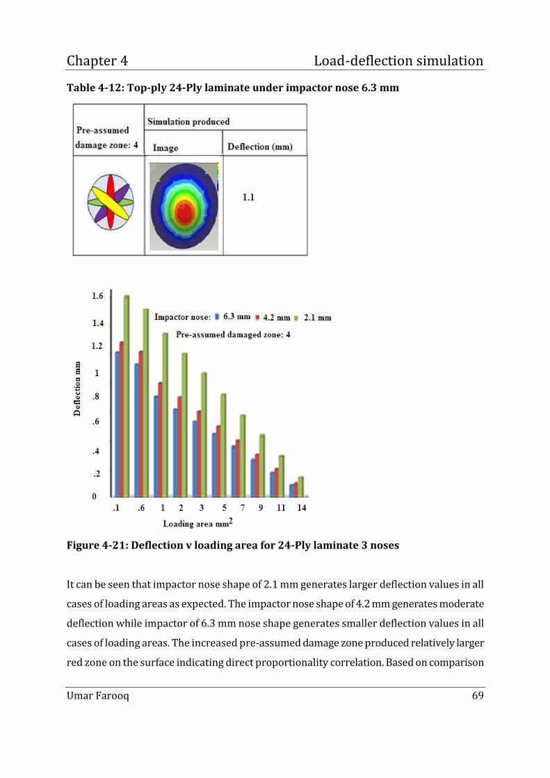
Chapter 4 Load-deflection simulation
Umar Farooq 69
Table 4-12: Top-ply 24-Ply laminate under impactor nose 6.3 mm
Figure 4-21: Deflection v loading area for 24-Ply laminate 3 noses
It can be seen that impactor nose shape of 2.1 mm generates larger deflection values in all
cases of loading areas as expected. The impactor nose shape of 4.2 mm generates moderate
deflection while impactor of 6.3 mm nose shape generates smaller deflection values in all
cases of loading areas. The increased pre-assumed damage zone produced relatively larger
red zone on the surface indicating direct proportionality correlation. Based on comparison

Chapter 4 Load-deflection simulation
Umar Farooq 70
of the results it can be argued that the pre-assumed damage induced simulation can be
used to correlate low velocity impact damage zone under various loads.
4.8 Impactor nose shape against through-thickness damage location
4.8.1 24-Ply laminate
Simulations were carried out for 24-Ply undamaged and laminates embedded with
successive damaged ply impacted from impactor noses. The selected simulated results for
24-Ply laminates are compared for 6.3 mm impactor in Figure 4-22(a), 4.2 mm impactor in
Figure 4-22(b), and 2.1 mm impactor in Figure 4-22(c). It can be seen from the charts
that the deflection values are higher at the beginning when pre-assumed damage was
located around outer surface of the laminate and were relatively smaller around the mid-
surface. Both the undamaged and pre-assumed damaged ply laminates show similar trends
in all the column charts. This indicates that effect of damage reduces when it is located
towards the mid-surface. Moreover, trends related to deflection values show inverse
proportionality to the impactor nose profiles.
a) Impactor nose 6.3 mm
Ply-by-ply location of damage location

Chapter 4 Load-deflection simulation
Umar Farooq 71
b) Impactor nose 4.2 mm
c) Impactor nose 2.1 mm
Figure 4-22: Deflection against damage location 24-Ply laminate v impactor nose

Chapter 4 Load-deflection simulation
Umar Farooq 72
4.8.2 16-Ply laminate
Simulations were carried out for 16-Ply undamaged and laminates embedded with
successive damaged ply impacted from impactor noses. The selected simulated results for
16-Ply laminates are compared for 6.3 mm impactor in Figure 4-23(a) 4.2 mm impactor in
Figure 4-23(b), and 2.1 mm impactor in Figure 4-23(c). It can be seen from the charts
that the deflection values are higher at the beginning when impactor nose radii were
relatively smaller. Both the undamaged and pre-assumed damaged ply laminates show the
same trends. However, the trends diminish as nose radii started to increase. Similar trend
observations can be seem from rest of the three bar charts. These trends lead that larger
deflection values are produced by the impactor of smaller nose profiles. As anticipated,
larger impactor nose profiles produced lesser deflection values that lead to the larger strain
energy absorbed by the laminates, less local damage, and larger internal global damage.
a) Impactor nose 6.3 mm

Chapter 4 Load-deflection simulation
Umar Farooq 73
b) Impactor nose 4.2 mm
c) Impactor nose 2.1 mm
Figure 4-23: Deflection against damage location for16-Ply laminate v impactor nose

Chapter 4 Load-deflection simulation
Umar Farooq 74
4.8.3 8-Ply laminate
Simulations were carried out for 8-, 16-, and 24-Ply undamaged and laminates embedded
with successive damaged ply impacted from impactor noses. The selected simulated results
for 8-Ply laminates are compared for 6.3 mm impactor in Figure 4-24(a), 4.2 mm impactor
in Figure 4-24(b), and 2.1 mm impactor in Figure 4-24(c). It can be seen from the charts
that the deflection values are higher at the beginning when impactor nose radii were
relatively smaller. Both the undamaged and pre-assumed damaged ply laminates show the
same trends. However, the trends diminish as nose radii started to increase. Similar trend
observations can be seem from rest of the three bar charts. These trends lead that larger
deflection values are produced by the impactor of smaller nose profiles. On the hand, larger
impactor nose profiles produced lesser deflection values that lead to the larger strain
energy absorbed by the laminates, less local damage, and larger internal global damage.
b) Impactor nose 6.3 mm

Chapter 4 Load-deflection simulation
Umar Farooq 75
c) Impactor nose 4.2 mm
c) Impactor nose 2.1 mm
Figure 4-24: Deflection against damage location for8-Ply laminate v impactor nose

Chapter 4 Load-deflection simulation
Umar Farooq 76
4.9 Summary
Pre-assumed damage induced load-deflection simulations were conducted for quasi-
isotropic impacted laminates. Simulations produced deflection values were correlated to
pre-assumed damage zones, loading areas, progressive damage against, through-thickness
locations, and impactor’s nose shape. Comparison of simulated results validated to the
experimental data and the results available in the literature up to (±12%) deviations. The
following conclusions can be were drawn from the results:
Central deflection values of undamaged and damaged laminates correlate to the transverse
loads. Loading area under impactors’ nose tip and size of impactor nose profiles were found
in inverse proportion to the predicted deflection quantities. Relatively small loading area
and impactor nose produced local indentation while large impactor nose profiles produced
larger global deflections on the surface.
Constant loading areas against accumulated damage under different impactor noses also
show inverse proportion against the deflection quantities.

Chapter 4 Load-deflection simulation
Umar Farooq 77
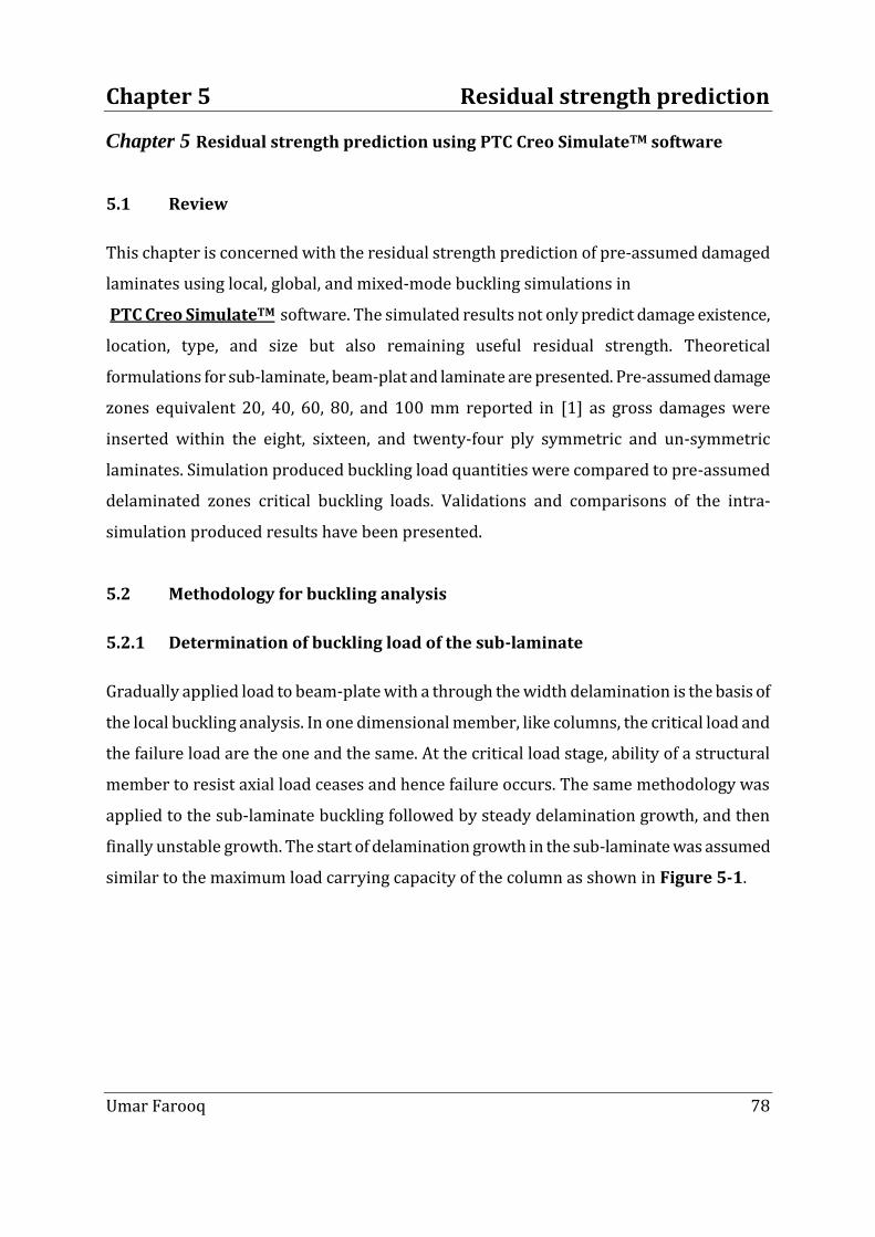
Chapter 5 Residual strength prediction
Umar Farooq 78
Chapter 5 Residual strength prediction using PTC Creo SimulateTM software
5.1 Review
This chapter is concerned with the residual strength prediction of pre-assumed damaged
laminates using local, global, and mixed-mode buckling simulations in
PTC Creo SimulateTM software. The simulated results not only predict damage existence,
location, type, and size but also remaining useful residual strength. Theoretical
formulations for sub-laminate, beam-plat and laminate are presented. Pre-assumed damage
zones equivalent 20, 40, 60, 80, and 100 mm reported in [1] as gross damages were
inserted within the eight, sixteen, and twenty-four ply symmetric and un-symmetric
laminates. Simulation produced buckling load quantities were compared to pre-assumed
delaminated zones critical buckling loads. Validations and comparisons of the intra-
simulation produced results have been presented.
5.2 Methodology for buckling analysis
5.2.1 Determination of buckling load of the sub-laminate
Gradually applied load to beam-plate with a through the width delamination is the basis of
the local buckling analysis. In one dimensional member, like columns, the critical load and
the failure load are the one and the same. At the critical load stage, ability of a structural
member to resist axial load ceases and hence failure occurs. The same methodology was
applied to the sub-laminate buckling followed by steady delamination growth, and then
finally unstable growth. The start of delamination growth in the sub-laminate was assumed
similar to the maximum load carrying capacity of the column as shown in Figure 5-1.

Chapter 5 Residual strength prediction
Umar Farooq 79
Figure 5-1: Schematic representation (1) sub-laminate and 2) column).
Assuming the sub-laminate is symmetrical then there will be no extension-bending
coupling, and the transverse displacement is governed by the one dimensional differential
equation.
𝝏𝟒𝒘
𝝏𝒙𝟒 +𝑷
𝑫
𝝏𝟐𝒘
𝝏𝒙𝟐 = 𝟎 (5-1)
Where P = buckling load per unit width, t = thickness and D = flexural rigidity of the
delaminated region, which equates to Et3/12.The general solution of Eq. (5-1) is
𝒘 = 𝑨 + 𝑩𝒙 + 𝑪𝒔𝒊𝒏𝜷𝒙 + 𝑫𝒄𝒐𝒔𝜷𝒙 (5-2)
The boundary conditions for the arrangement are: w = w/x = 0 at x = 0 and w = w/x =
0 at x = a.
Applying the boundary conditions gives the following equations for determining the
constants in Eq. (5-2).

Chapter 5 Residual strength prediction
Umar Farooq 80
𝑨 + 𝑫 𝟎 𝟎 𝟎 𝟎 = 𝟎𝑩 + 𝑪𝜷 𝟎 𝟎 𝟎 𝟎 = 𝟎𝑨 + 𝑩𝒂 + 𝑪𝒔𝒊𝒏𝜷𝒂 + 𝑫𝒄𝒐𝒔𝜷𝒂 = 𝟎𝑩 + 𝑪𝜷𝒄𝒐𝒔𝜷𝒂 − 𝑫𝜷𝒔𝒊𝒏𝜷𝒂 𝟎 𝟎 = 𝟎
(5-3)
The only way to have a nontrivial solution is to set the determinants of the coefficients
equal to zero.
𝟏 𝟎 𝟎 𝟏𝟎 𝟏 𝜷 𝟎𝟏 𝒂 𝒔𝒊𝒏𝜷𝒂 𝒄𝒐𝒔𝜷𝒂𝟎 𝟏 𝜷𝒄𝒐𝒔𝜷𝒂 −𝜷𝒔𝒊𝒏𝜷𝒂
(5-4)
Setting the determinant equal to zero gives the following equation
𝟐 𝒄𝒐𝒔𝜷𝒂 − 𝟏 + 𝜷𝒂𝒔𝒊𝒏𝜷𝒂 = 𝟎
𝒔𝒊𝒏𝜷𝒂 = 𝟐𝒔𝒊𝒏 𝜷𝒂
𝟐 𝒂𝒏𝒅 𝒄𝒐𝒔𝜷𝒂 = 𝟏 − 𝟐𝒔𝒊𝒏𝟐
𝜷𝒂
𝟐
can be written in the form
𝒔𝒊𝒏𝜷𝒂
𝟐 𝜷𝒂
𝟐𝒄𝒐𝒔
𝜷𝒂
𝟐− 𝒔𝒊𝒏
𝜷𝒂
𝟐 (5-5)
One solution of the equation is, 𝒔𝒊𝒏𝜷𝒂
𝟐= 𝟎
Therefore 𝜷𝒂 = 𝟐𝝅 or
𝜷𝟐 = 𝟒𝝅𝟐
𝒂𝟐 (5-6)
The buckling load is related to the parameter by
𝑷 = −𝜷𝟐𝑫 (5-7)
Substituting Eq. (5-6), the flexural rigidity and the width of the delamination, ‘b’ into
Eq. (5-7) gives
𝑷∗ = −𝟒𝑫𝝅𝟐
𝒂𝟐 = −𝑬𝒃𝒕𝟑𝝅𝟐
𝟑𝒂𝟐 (5-8)
Where 𝑷∗ is equal to the buckling load for the entire laminate
The simulated buckling loads at each ply interface through to the mid-plane of the
laminates with various pre-assumed delamination zone diameters is shown in Table 5-1.

Chapter 5 Residual strength prediction
Umar Farooq 81
Table 5-1: Ply-by-ply local buckling load KN
Thickness location
mm
Pre-assumed damage zone
diameter mm
20 40 60 80 100
Buckling load KN
.12 10 10 5 3 2
.24 15 12 6 4 3
.36 22 13 8 6 4
.48 24 15 10 8 5
0.6 26 16 12 10 6
0.72 28 20 12 8 6
0.84 39 24 15 10 8
0.96 45 24 15 12 8
1.08 80 30 20 15 10
1.2 90 35 22 18 12
1.32 90 35 22 18 12
1.44 90 35 22 18 12
5.2.2 Determination of buckling load of laminated plate
Failures in plates do not occur when the critical buckling load is reached. Plates continue to
resist the in-plane loads excessive to the critical load before failure. Thus the post-buckling
behaviour of plates plays an important role in determining the ultimate load carrying
capacity of plates. The having laminate cut-out is shown in Figure 5-2 (a). The local and
global buckling simulated modes are inserted here to clarify the difference between local
buckling in Figure 5-2 (b) and global mode in Figure 5-2 (c).
Chapter 5 Residual strength prediction
Umar Farooq 82
Figure 5-2: Bending and compression acting on a delaminated orthotropic plate: a)
Theoretical, b) Local buckling, and c) Global buckling modes
For sub-laminate of thickness h, the delamination can be calculated assuming the forces Ny
= Nxy = 0, and bending My = Mxy = 0 then 2
hTNM x
x
.
Solving for the mid-surface strains and curvatures and calculating the ply strains and
stresses the maximum compressive stresses in the 0o ply direction can be compared with
those for an undamaged case. The model predicted a 67% reduction in strength compared
to 61% from the experiments for a carbon fibre/epoxy laminate [1].
Procedure of obtaining the critical value of load for a plate elements is an extension to the
two-dimensions and exactly similar as described for the columns. Adding up the
contribution of the in-plane as well as out-of-plane forces and momentums yield the
required thin rectangular plate buckling equation:
𝜵𝟒𝒘 = 𝟏
𝑫 𝒒 + 𝑵𝒙
𝝏𝟐𝒘
𝝏𝒙𝟐 +𝟐𝑵𝒙𝒚𝝏𝟐𝒘
𝝏𝒙𝝏𝒚+ 𝑵𝒚
𝝏𝟐𝒘
𝝏𝒚𝟐 (5-9)
With substitutions: transverse loading ‘q’ = 0 and in-plane loading: 𝑁𝑥 = − 𝑁1; 𝑁𝑦 = − 𝑁2;
and 𝑁𝑥𝑦 = − 𝑁12as constants. The Eq. (5-9) for isotropic plate becomes
𝜵𝟒𝒘 +𝟏
𝑫 𝑵𝟏
𝝏𝟐𝒘
𝛛𝒙𝟐 +𝟐𝑵𝟏𝟐𝝏𝟐𝒘
𝝏𝒙𝝏𝒚+ 𝑵𝟐
𝝏𝟐𝒘
𝝏𝒚𝟐 = 𝟎 (5-10)

Chapter 5 Residual strength prediction
Umar Farooq 83
In case of fibre reinforced constructions analysis lead to the development of advanced
model of a general laminate element as shown in Figure 3-1. The laminate consists of ‘N’
layers thick and is symmetrical in both geometry and material about its central surface.
The subscript k indicates layer number t denotes thickness of a ply, and h denotes thickness
of the laminate. Distance from middle surface to inner surface of the kth ply is denoted by
𝑍𝑘−1and corresponding distance from middle surface to outer surface is denoted by 𝑍𝑘 . In-
plane forces: Nx, Ny and Nxy and the out-of-plane deflections w can be used to formulate
buckling behaviour as:
𝑫𝒙𝝏𝟒𝒘
𝝏𝒙𝟒 + 𝟐𝑯𝝏𝟒𝒘
𝝏𝒙𝟐𝝏𝒚𝟐 + 𝑫𝒚𝝏𝟒𝒘
𝝏𝒚𝟒 + 𝑵𝟏𝝏𝟐𝒘
𝝏𝒙𝟐 +𝟐𝑵𝟏𝟐𝝏𝟐𝒘
𝝏𝒙𝝏𝒚+ 𝑵𝟐
𝝏𝟐𝒘
𝝏𝒚𝟐 = 𝟎 (5-11)
Where:𝐷𝑥 𝑎𝑛𝑑 𝐷𝑦 are the flexural-rigidities along x and y directions respectively, and H is
the effective torsional rigidity. The critical buckling load can be calculated for the simply
supported plate at x = 0, x = a; and at y = 0, y = b subjected to uniaxial compressive load per
unit length (𝑁1) with 𝑁2 = 𝑁12 = 0. Deflection shape is assumed by a double sine series as:
𝒘 = 𝒘𝒎𝒏𝒔𝒊𝒏𝜶𝒎𝒙 𝒔𝒊𝒏𝜷𝒏𝒚∞𝒏
∞𝒎 (5-12)
𝑤ℎ𝑒𝑟𝑒: 𝜶𝒎 = 𝒎𝝅
𝒂 , 𝜷𝒏 =
𝒏𝝅
𝒃 (5-13)
and 𝑤𝑚𝑛 are the coefficients of the series Eq. (5-12).
Substituting Eq. (5-12) into Eq. (5-11) and taking common 𝑤𝑚𝑛 𝑠𝑖𝑛𝛼𝑚𝑥 𝑠𝑖𝑛𝛽𝑛𝑦 yields:
𝑫𝒙𝜶𝒎𝟒 + 𝟐𝑯𝜶𝒎
𝟐 𝜷𝒏𝟐 + 𝑫𝒚𝜷𝒏
𝟒 − 𝜶𝒎𝟐 𝑵𝟏 = 𝟎. This may be written as
𝑵𝟏 =𝟏
𝜶𝒎𝟐 𝑫𝒙𝜶𝒎
𝟒 + 𝟐𝑯𝜶𝒎𝟐 𝜷𝒏
𝟐 + 𝑫𝒚𝜷𝒏𝟒 and simplifying Eq. (5-13) may put as
𝑵𝟏 =𝝅𝟐𝒂𝟐
𝜶𝒎𝟐 𝑫𝒙
𝒎𝟒
𝒂𝟒+ 𝟐𝑯
𝒎𝟐𝒏𝟐
𝒂𝟐𝒃𝟐+
𝒎𝟒
𝒂𝟒𝑫𝒚
Multiplying the numerator and the denominator by 𝑏2𝑎2
𝑚2 and simplify to give
𝑵𝟏 =𝝅𝟐
𝒃𝟐 𝒎
𝒄 𝟐
𝑫𝒙 + 𝟐𝑯𝒏𝟐 + 𝒄
𝒎 𝟐
𝒏𝟒𝑫𝒚
Where: c = aspect ratio = a/b
Multiplying both the numerator and the denominator by 𝐷𝑥𝐷𝑦 1
2 and simplify to give

Chapter 5 Residual strength prediction
Umar Farooq 84
𝑵𝟏 =𝝅𝟐 𝑫𝒙𝑫𝒚
𝟏𝟐
𝒃𝟐 𝒎
𝒄 𝟐
𝑫𝒙/𝑫𝒚 𝟏
𝟐 +𝟐𝑯𝒏𝟐
𝑫𝒙𝑫𝒚 𝟏
𝟐 +
𝒄
𝒎 𝟐
𝒏𝟒 𝑫𝒙/𝑫𝒚 𝟏
𝟐 𝒄
𝒎 𝟐
𝒏𝟒 𝑫𝒙/𝑫𝒚 𝟏
𝟐
(5-14)
For the value of n =1, N1 will assume the minimum value, i.e., the laminate will buckle along
y-direction as a single half-wave. This makes the Eq. (5-14) to assume the form,
𝑵𝟏 =𝝅𝟐 𝑫𝒙𝑫𝒚
𝟏𝟐
𝒃𝟐 𝒎
𝒄 𝟐
𝑫𝒙/𝑫𝒚 𝟏
𝟐 +𝟐𝑯
𝑫𝒙𝑫𝒚 𝟏
𝟐 +
𝒄
𝒎 𝟐
𝒏𝟒 𝑫𝒙/𝑫𝒚 𝟏
𝟐 𝒄
𝒎 𝟐
𝑫𝒙/𝑫𝒚 𝟏
𝟐
(5-15)
The value of ‘m’, the half-wave along x-direction, can be obtained on minimizing N1 with
respect to ‘m’ for the case when the aspect ratio ‘c’ is an integer number.
Thus,𝝏𝑵𝟏
𝝏𝒎= 𝟎 𝒈𝒊𝒗𝒆𝒔:
𝟐𝒎
𝒄𝟐 𝑫𝒙/𝑫𝒚
𝟏𝟐 =
𝟐𝒄𝟐
𝒎𝟑 𝑫𝒙/𝑫𝒚
𝟏𝟐 or
𝒄 = 𝒎 𝑫𝒙/𝑫𝒚 𝟏
𝟒 (5-16)
With Eq. (5-16) the critical compressive load in Eq. (5-17) can be written as
𝑵𝟏, 𝒄𝒓 =𝟐𝝅𝟐 𝑫𝒙𝑫𝒚
𝟏𝟐
𝒃𝟐 𝟏 +𝑯
𝑫𝒙𝑫𝒚 𝟏
𝟐 (5-17)
On substituting 𝐷𝑥 = 𝐷𝑦 = 𝐻 = 𝐷 plate rigidity Eq. (5-15) reduces to the isotropic case
𝑵𝟏, 𝒄𝒓 =𝟒𝝅𝟐𝑫
𝒃𝟐
For the general case when the aspect ratio is not an integer, the wave parameter, ‘m’ can be
determined on the identical lines as for isotropic case. Re-writing the Eq. (5-15) as
𝑵𝟏 = 𝑲𝝅𝟐 𝑫𝒙𝑫𝒚
𝟏𝟐
𝒃𝟐 (5-18)
Where:
𝑲 = 𝒎
𝒄 𝟐
𝑫𝒙/𝑫𝒚 𝟏
𝟐 +𝟐𝑯𝒏𝟐
𝑫𝒙𝑫𝒚 𝟏
𝟐 +
𝒄
𝒎 𝟐
𝑫𝒙/𝑫𝒚 𝟏
𝟐 (5-19)
Applying aspect ratio reasoning, Eq. (5-19) may be expressed as
𝑫𝒙 𝒎
𝒄 𝟐
+ 𝟐𝑯 + 𝑫𝒚 𝒄
𝒎 𝟐
= 𝑫𝒙 𝒎+𝟏
𝒄 𝟐
+ 𝟐𝑯 + 𝑫𝒚 𝒄
𝒎+𝟏 𝟐
(5-20)
Equation (5-20) may be simplified to calculate aspect ratios:
𝒄 = 𝒎 𝒎 + 𝟏 𝟏
𝟐 𝑫𝒙/𝑫𝒚 𝟏
𝟐 (5-21)

Chapter 5 Residual strength prediction
Umar Farooq 85
It can be readily verified that Eq. (5-21) reduces to the case for isotropic plates 𝐷𝑥 = 𝐷𝑦 =
𝐷. The number ‘m’ corresponding to a given value of the aspect ratio ‘c’ of the plate can be
obtained on the identical line as for the isotropic case. That is for
𝟎 < 𝒄𝟐 < 2 𝑫𝒙/𝑫𝒚 𝟏
𝟐 , m =1
𝟐 𝑫𝒙/𝑫𝒚 𝟏
𝟐 < 𝒄𝟐 < 6 𝑫𝒙/𝑫𝒚 𝟏
𝟐 , m = 2
𝟔 𝑫𝒙/𝑫𝒚 𝟏
𝟐 < 𝒄𝟐 < 12 𝑫𝒙/𝑫𝒚 𝟏
𝟐 , m = 3
(5-22)
and so on.
The lowest of the two values indicates the mode in which buckling occurs. In the case of
elliptical shaped damage which is not oriented on axes coinciding with the global x and y
axes, a new set of local coordinates oriented to the elliptical transformation can be defined.
From Eq. (5-18) calculated buckling for various boundary conditions is listed in Table 5-2.
Table 5-2: Results of theoretical calculated buckling load
Boundary condition Parameter K Buckling load ‘Nxb’ KN
Simply supported 3.5 43. 46.56
Fully clamped 7.45 91.54 99.11
Edges b simply supported,
edges a clamped
5.78
71.02 76.89
Edges a simply supported,
edges b clamped
4.72 57.99 62.79
For the not especially orthotropic laminates the fibres are not aligned with the principal
plate axis (x, y) then the method does indicate to accommodate the changes. In this case the
loads 𝑁𝑦 = 𝑁𝑥𝑦 = 𝑞 𝑥, 𝑦 = 0 and the bending-twist couplings terms are: 𝐷16 = 𝐷26 = 0.
Solving Eq. (5-23) provides coefficient 𝐾0 :
𝑲𝟎 = 𝒂
𝒃 𝑫𝟐𝟐
𝑫𝟏𝟏 𝟏
𝟒
(5-23)

Chapter 5 Residual strength prediction
Umar Farooq 86
Once 𝐾0 is determined solution of Eq. (5-24) provides the theoretical buckling load 𝑁𝑥𝑏 :
𝑵𝒙𝒃 = 𝑲𝟎
𝑫𝟐𝟐𝑫𝟏𝟏
𝟏𝟐
𝒃𝟐 +𝑪𝝅𝟐𝑫𝟎
𝒃𝟐 (5-24)
Where C = coefficient dependent upon plate edge conditions and 𝐷0 = 𝐷12 + 2𝐷33 . Using
Eq. (5-24) calculated buckling load values obtained for various boundary conditions are
presented in Table 5-3.
Table 5-3: Results of theoretical calculations based on Eq. (5-24)
Boundary condition Parameter K Buckling load ‘Nxb’ KN
Simply supported 3.5 45 47
Fully clamped 7.45 109 105
Edges b simply supported,
edges a clamped
5.78
81 81
Edges a simply supported,
edges b clamped
4.72 70. 69
The comparison of both the cases shows that the laminate buckling loads is slightly higher
than the isotropic plat for the same geometry and boundary conditions. This is attributed to
the laminate stiffness in the direction of loading to be higher than the isotropic. Presented
results could be compared to the finite element model and to the test laminates against
different flexural stiffness values. .
5.3 Pre-assumed de-lamination induced buckling analysis
Damage tolerance from damage and delamination induced buckling analysis is an
important failure mechanism where through-thickness properties of laminates degrade by
low velocity drop-weight impact. Poor post-impact compressive strength is the greatest
weakness of composite laminates. This is mainly due to local instability resulting from
Chapter 5 Residual strength prediction
Umar Farooq 87
delamination causing large reductions in compressive strength. Standard Test Method for
Compressive Residual Strength Properties of Damaged Polymer Matrix Composite Plates
methods (ASTM: D7317) is being widely used to evaluate residual strength. One of the
inherent concerns in interpreting test results is the difference in standards used to measure
the performance. The results are difficult to translate from one to the other, and subtle
variations in the support conditions have shown to cause large changes in the final results.
Moreover, experimental methods are limited, time and resource consuming. Currently, no
recognized international standard test method exists. Similar specifications produced by
major organizations do differ in details: laminate size, impact conditions, anti-buckling
guides, end tabs/grips. There clearly exists the need to be able to predict the tolerance of
structures to damage forms which are not readily detectable [59]. Efficient simulation
analysis was desired to validate the experimental study and to evaluate compressive
residual strength that includes mixed-mode buckling effects. Buckling failure in laminates
occurs well below the predicted allowable limits normally predicted by failure criteria. The
methodology of inserting pre-assumed de-laminated zones to predict residual strength
after impact was found relevant and selected for this investigation.
5.3.1 Finite element meshing schemes
The carbon fibre test specimens of dimensions: 150 mm x 120 mm x 2.88 mm eight,
sixteen, and twenty-four laminates of lay-up codes: [45/0/-45/90]S, [45/0/-45/90]2S,
and [45/0/-45/90]3S test by James [1] were considered. The model is representative of
the full-scale test specimen with the dimensions shown in Figure 5-3. A mesh was
generated with 40 elements across the width, 50 elements down the length and 8
elements thick. A single element thickness was equivalent to three ply thicknesses (0.36
mm). This equated to 16,000 brick elements with an aspect ratio of 3 : 0.36
(length/thickness = 8.33). The solid element deemed computationally intensive.

Chapter 5 Residual strength prediction
Umar Farooq 88
Figure 5-3: Finite element model representation
Hence shell element was selected and used throughout for the buckling analysis. Industry
provided orthotropic material proposed in [1] was assigned to the elements with the
mechanical properties listed in Table 4-1. The properties are taken from the mechanical
test results presented in [1] with the exception of the inter-laminar shear modulus (G23)
calculated using simple theory: 23
223
12
EG where, E2 = transverse ply modulus and 23 =
through the thickness Poisson’s ratio. Once the material properties were assigned the local
element orientation was defined in terms of the global axes. Each layer of elements through
the thickness was treated as a single ply although they actually as previously mentioned
accounted for three plies. To simulate the required overall laminate stiffness the
orientation of each ply in the model was rotated to align the major ply mechanical
properties with the principal fibre directions in the laminate. The simulated lay-up in the
model was therefore [45/0/-45/90/90/-45/0/45]. For the base complete axial and
rotational restraints were applied to the bottom edge (shell element). On the top surface
and two side surfaces an axial restraint in the Z direction and full rotational restraints were
applied. This would allow displacements in the X and Y directions and provide an
approximation of the buckling mode shape seen. Considering the plate in a typical circle of

Chapter 5 Residual strength prediction
Umar Farooq 89
radius 20 mm was marked at the centre of the model for comparison of undamaged and
damage simulation effects as shown in Figure 5-4. Dimensions are defined by three
parameters: length a, width b and thickness h. The circular cross-hatched area indicates the
damage zone of diameter d. The origin of the Cartesian coordinate system is located at a
corner of the plate. Its x-axis is parallel to the short edges, while the y-axis is parallel to the
long edges. The compressive load is applied on the top edge. The compressive load F is
applied on top edge parallel along middle plane of the laminate plate. The horizontal in-
plane displacement, the vertical in-plane displacement and the out-of-plane displacement
are denoted as u, v and w, respectively. The laminate was clamped at the bottom edge.
Extensional constraints were applied at the top edge in the in-plane direction with
rotational constraint in y-direction. The other two sides were fixed in x- and z-directions.
Plane dimensions of laminates remained the same in all the cases. All four edges remain
straight when the plate is deformed. A computer created model is presented in Figure
5-4(a). The symbol R (Rx, Ry, & Rz) indicates rotations with respect to reference axis while a
indicates width and b denotes length of the desired laminate change with specific size.
Simulation generated undamaged laminate is shown in Figure 5-4 (b).
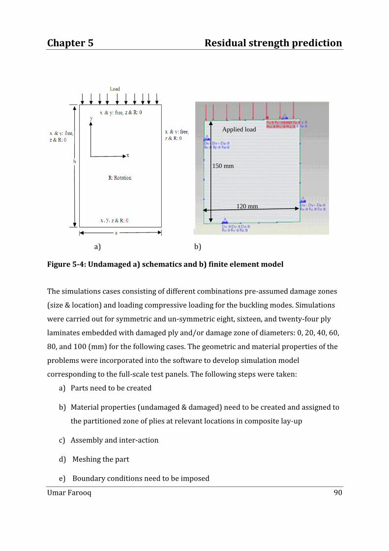
Chapter 5 Residual strength prediction
Umar Farooq 90
a) b)
Figure 5-4: Undamaged a) schematics and b) finite element model
The simulations cases consisting of different combinations pre-assumed damage zones
(size & location) and loading compressive loading for the buckling modes. Simulations
were carried out for symmetric and un-symmetric eight, sixteen, and twenty-four ply
laminates embedded with damaged ply and/or damage zone of diameters: 0, 20, 40, 60,
80, and 100 (mm) for the following cases. The geometric and material properties of the
problems were incorporated into the software to develop simulation model
corresponding to the full-scale test panels. The following steps were taken:
a) Parts need to be created
b) Material properties (undamaged & damaged) need to be created and assigned to
the partitioned zone of plies at relevant locations in composite lay-up
c) Assembly and inter-action
d) Meshing the part
e) Boundary conditions need to be imposed
120 mm
150 mm
Applied load

Chapter 5 Residual strength prediction
Umar Farooq 91
The eight, sixteen, and twenty-four plies circular laminates were incorporated in the finite
element developed models for all the numerical analyses. Laminate was meshed with
general purpose linear fully integrated quadrilateral conventional shell elements: 895 and
reduced integration triangular conventional shell elements: 75 using two different levels of
refinement. Each laminate ply is modelled with deformable one shell element through-the-
thickness which behaves according to the continuum damage model. Total number of
element for a laminate can be obtained by multiplying the number of plies. Fine meshes
were created in regions where a more reliable prediction of the damage initiation load is
required. The impact damage zone where damage takes place requires the smaller
elements that allow better simulation of the stress distributions at the mesh-transition
regions. In regions away of the impact zone where damage is not expected to occur or its
initiation load is not critical course meshes were created. It was necessary to re-mesh
central portions of the problem domain in order to accommodate the changes of the
degraded material properties (discontinuities). A typical circle of diameter 20 (mm)
created at the centre of the model is shown in Figure 5-5 (a). Shape and size of the circle
can be changed according to the pre-assumed damage zones. Shell element was selected
and used throughout for the simulations. Computer generated meshed model is shown in
Figure 5-5 (b)-(e). Restraints were applied to all the four sides. Completer axial and
rotational restraints were already applied to the bottom edge. On the top and the other two
side edges an axial restraint in the z direction and full rotational restraints were applied.
The model allows displacements in the x and y directions and provides an approximation of
the buckling mode shape seen on tests in [1]. Before proceeding with the buckling analysis
tests for undamaged laminates were performed to calibrate the finite element model under
compressive pressure loading Figure 5-5 (f). Once simulation produced data was deemed
satisfactory the same model was modified for damaged zones inserted at various locations
through-thickness under variable loading from 10-50 KN to accommodate cases of global,
local, mixed-mode buckling.

Chapter 5 Residual strength prediction
Umar Farooq 92
Figure 5-5: a) Un-meshed, b) Course meshed, c) Mapped mesh, d) Fine meshed, and e) Loaded and fine meshed
5.3.2 Simulation of un-damaged laminate
Before proceeding with the buckling analysis of damaged laminates, simulations of
undamaged laminates were performed. The un-damage material properties assigned to the
zone are given in Table 4-4 while degraded materials assigned to the zone are given Table
4-2. The simulation produced results were compared to analytical calculation to calibrate
the finite element model under pressure load of 50 KN proposed in [1] applied to the top
surface as both axial and rotational restraints were applied to the bottom surface. Once the
setup of the model was deemed satisfactory the loading was changed to an arbitrary
pressure load of 10 KN to 50 KN applied across the top surface. Initial work was performed
to verify the element suitability of the simple models with various mesh densities and
boundary conditions.

Chapter 5 Residual strength prediction
Umar Farooq 93
5.3.3 Simulation of damaged laminate
After successful completion of un-damaged laminates simulations, pre-assumed damage
zones were inserted in the laminates. Experimental studies consistently report that damage
and delamination occur at interfaces between plies with different orientations. Moreover,
with increasing impact energy the localised area suffers increasing amounts of damage in
the form of matrix cracks, delamination, fibre pullout and fibre fracture, which precipitate
outward. The failure mechanisms under compression are particularly difficult to assess. In
an impact damaged specimen delaminations of different sizes occur through the thickness.
In order to allow predictions of strength reduction an assumption that although impact
damage consists of many fibre cracks and delaminations only some of these can be active in
controlling the residual strength that approximate the damage as a gross damage area.
Gross damage areas recorded during the impact testing of the carbon fibre/epoxy laminate
ranged from 500 mm2 to 8800 mm2 and were circular in shape reported in [1], Figure 4-5
and Figure 4-6. The damage induced buckling was in two formats with a symmetrical
delamination, which required the removal of two through the thickness elements at the mid
plane, similar to the removal of a section of two simulated plies at the mid plane Figure
5-6. The second was the removal of a single through the thickness element to one side of
the mid plane Figure 5-7. That produced an unbalanced condition locally and may cause
failure by a different mode.

Chapter 5 Residual strength prediction
Umar Farooq 94
Figure 5-6: Double delamination simulation at the mid-plane [1]
Figure 5-7: Single delamination simulation at the mid-plane [1]

Chapter 5 Residual strength prediction
Umar Farooq 95
Approximate values of the pre-assumed damage zones determined for gross damage using
were within the acceptable range. Moreover, to simplify the analysis and compare with the
test findings [1] the model simulated circular damage with diameters ranging from 20 mm
to 100 mm in 20 mm steps corresponding to gross pre-assumed damage zones: 314, 1257,
2827, 5027, and 7854 mm2 were considered. Degradation material properties given in as
delaminated zones were used in simulations to study effects of the delamination buckling
behaviour. Thickness of the damage zone was considered to be equivalent to a single ply.
Through-thickness locations of the damage zones varied from top to bottom for un-
symmetric lay-ups and from top to the halfway through for the symmetric lay-ups.
5.4 Validation of selected buckling analysis methodology
5.4.1 Influence of pre-assumed de-laminated zone on buckling load
Before proceeding with the planned buckling simulation cases, simulation of undamaged
laminates were carried out to validate the experimental data and to calibrate the finite
element model developed for the current investigation. Moreover, to create a baseline for
comparison of the simulation generated results mode. Selected simulated results obtained
from increasing size of pre-assumed damaged zones are compared against corresponding
results available in. Comparisons of buckling loads for 8-Ply and 24-Ply laminates are
shown in Figure 5-8 (a) [1] against Figure 5-8 (b). The plots show predicted 90 KN load
for un-damaged 8-Ply laminates. Comparison of predicted buckling load for 24-Ply
laminates is also within acceptable range 80-90 KN. These values agree well when
compared to the effective elastic constants from buckling loads in Table 5-2 and Table 5-3.
This indicates that un-damaged or smaller delamination size laminates buckle under
relatively larger loads.

Chapter 5 Residual strength prediction
Umar Farooq 96
Figure 5-8: Residual strength v damaged zone (a) and b) Simulated
On the other hand, stability of the laminate reduces dramatically as delaminated zones are
increased. Growth of de-laminated zones adversely affects stability of the residual strength
of structures. As the delamination becomes more and more severe, the drop is slow down
and come to a smooth stop till the delamination spread across the entire laminate. It
indicates that the laminate does not loss all its load carrying capacities but has some
residual stiffness. This happens under limit condition delamination divides the laminate
into two sub-laminates. Residual stiffness of the laminate in such case is measured by the
stiffness of the thinner sub-laminates. Consistent comparison of results indicate that
simulation produced buckling results are reliable. Moreover, plots show insignificant
difference between 8- and 24-Ply lay-ups (different number of plies in a laminate).
5.4.2 Influence of delamination depth (location) on buckling load
Simulations were carried out to compare influence of the damage zone against buckling
load ply locating damage up to the mid-plane. Comparisons of delaminated zone locations
and buckling loads are shown in Figure 5-9 (a) against Figure 5-9 (b). Buckling load
shows proportional increase in buckling load corresponding to the location of the induced
de-laminated zone. Significant effects of the delaminated zones have been observed as

Chapter 5 Residual strength prediction
Umar Farooq 97
damage moves towards the mid-plane. Consistent results comparisons affirmed that
simulation can produce generate reliable data for buckling analysis.
Local buckling simulation
Simulated Experimental
Damage zone diameter (mm) Damage zone diameter (mm)
Through-thickness location (mm)
0 0.2 0.4 0.6 0.8 1 1.2 1.4 0 0.2 0.4 0.6 0.8 1 1.2 1.4
Through-thickness location (mm)
0 2
0
40
6
0
80
10
0
1
20
14
0
0 2
0
40
6
0
80
10
0
1
20
1
40
Bu
ckli
ng
lo
ad
(K
N)
Bu
ckli
ng
lo
ad
(K
N)
a) b)
Figure 5-9: Buckling load v through-thickness location (a) and b) Simulated)
To further clarify ambiguity in plot of Figure 5-9 (b) selected results from re-simulations
are shown in Table 5-4. The results are also compared to calculated values Table 5-1. It
can be seen from that as the pre-assumed damage zone 314 mm2 is located towards mid-
plane results in higher buckling load. All the buckling loads at each ply interface to the mid-
plane of the laminate with rest of the damage zones show failure in Table 5-4.

Chapter 5 Residual strength prediction
Umar Farooq 98
Table 5-4: Ply-by-ply local buckling load (KN)
Comparisons of results validated and confirmed that the simulation produced results are
genuine and model capable to simulate un-damaged and damaged laminates.
5.5 Comparison of intra-simulation results
5.5.1 Constant sized pre-assumed delaminated zone
Comparison of the buckling load against through-thickness position of the delaminated
zones of diameter 40 mm for 8-, 16-, and 24-Ply laminates further clarifies that simulation
produced results are consistent. Standard specimens of: 8-, 16-, and 24-Ply laminates of
identical thickness are shown in Figure 5-10.
Thickness location
(mm)
Pre-assumed damage zone (mm2)
314 1257 2027 5027 7854
Buckling load (KN)
.12 10 10 5 3 2
.24 15 12 6 4 3
.36 22 13 8 6 4
.48 24 15 10 8 5
0.6 26 16 12 10 6
0.72 28 20 12 8 6
0.84 39 24 15 10 8
0.96 45 24 15 12 8
1.08 80 30 20 15 10
1.2 90 35 22 18 12
1.32 90 35 22 18 12
1.44 90 35 22 18 12

Chapter 5 Residual strength prediction
Umar Farooq 99
Figure 5-10: Schematics of 8-, 16-, and 24-ply specimens
Difference between local and global mode shapes is shown through bar chart in Figure
5-11. Laminates were considered of uniform thickness to compare difference at ply level
thickness where 8-Ply laminate consists of 0.36 mm (equal to 3 ply thickness) thick plies
while 24-Ply laminate consists of 0.12 mm thick plies. Hence, 8-Ply laminates requires
higher load to buckle compared to 16 and 24-Ply laminates. As anticipated the buckling
load significantly increases as the delaminated zone moves towards the mid-plane.

Chapter 5 Residual strength prediction
Umar Farooq 100
Figure 5-11: Buckling load v location of de-laminated zone diameter (mm)
5.5.2 Increasing pre-assumed damage zones
Simulations were carried out for multiple delamination zones by increasing delaminated
zone diameters from 0, 20, 40, 60, 80 and 100 mm. Gross circular damage shapes were
supported in the forementionded simulated images and significant delamination size effect
on buckling load can be seen for 8-, 16-, and 24-Ply in columncharts shown in Figure 5-12.
Buckling loads show proportional reduction with pre-assumed damage zones for all three
lay-ups.
Figure 5-12: Buckling load v damage zone for 8-, 16- & 24-Ply laminate

Chapter 5 Residual strength prediction
Umar Farooq 101
5.5.3 Symmetric and un-symmetric lay-ups
Generally un-symmetric sub-laminate exhibit bending stretching coupling in out-out-plane
displacements before any kind of buckling occurs. In-plane twisting in the buckling mode
arises due to the presence of the non-zero D16 and D26 terms indicating a coupled behaviour
upon buckling, where the structure must twist in order to bend. Symmetric and un-
symmetric laminates were simulated with increasing damaged zones. Selected results for
24-Ply laminates compared in column chart shown in Figure 5-13. The column chart
shows insignificant difference between symmetric and un-symmetric laminates were also
simulated with constant damaged zones.
Figure 5-13: Buckling load v damage zone
Simulation produced results from pre-assumed damaged zone of 60 mm diameter at
different through-thickness locations are shown in column chart of Figure 5-14. Laminates

Chapter 5 Residual strength prediction
Umar Farooq 102
of the un-symmetric lay-ups induced with delaminated zone buckle at loads slightly lower
than the symmetric lay-ups. No significant difference can be seen from the column chart for
the both types of lay ups. Such anisotropic effects in composites have been under
investigation by various authors such as [15] and [18]. The comparison indicates consistent
results produced by the model.
Figure 5-14: Buckling load v through-thickness location damage area
The validity of the selected method of analysis was investigated via comparison of a range
of results available in the literature (even though the availability of such data in the
literature was scarce) and intra-simulations. Simulated values are plotted in column charts
for the lay-ups at various locations. Comparisons of the simulated local buckling loads for
the three lay-ups are within acceptable range (±12%) deviations. After simulation
generated results were deemed satisfactory, the extensive simulations for the intended
cases were carried out.

Chapter 5 Residual strength prediction
Umar Farooq 103
5.6 Numerical results and discussions
To examine the effect of low velocity impact damage as the pre-assumed delamination zone
on the buckling performance of the laminate, series of simulations were conducted.
Flowchart depicting cases of buckling simulation is shown in Figure 5-15.
Figure 5-15: Flowchart for damage tolerance analysis
5.6.1 Global buckling analysis
5.6.1.1 Simulation of hole laminate
In predicting critical load from global buckling analysis entire domain of the plate was
included in the simulations. The first case comprises of laminate containing relatively
larger internal holes (75% thickness) of laminate. Holes were created by removing circular
parts of increasing sizes from the laminate. Pre-assumed damage zones were introduced by
removing the areas equal to single ply thickness at the central position of the laminate (x, y)
= (75, 60) Figure 5-16.

Chapter 5 Residual strength prediction
Umar Farooq 104
Figure 5-16: Schematics of laminate embedded within a hole
All pre-assumed removed zones: 0, 314, 1257, 2827, 5027, and 7854 mm2 areas were
simulated for global buckling analysis laminates of 8, 16, and 24 plies. Selected comparison
of contour plots of 8-Ply laminate with buckling mode shapes are presented in images
Figure 5-17 (a)-(e). The initial out-of-plane deflection results in the formation of a natural
bending moment at the un-delaminated structure [59] which deflects in the same sense as
the delaminated layer. With increased damaged zone the buckling mode substantially grow
separating the contour plot across the thickness into two regions.The mid-planes separated
from each other and move in opposite directions. It can be seen that the delaminated zone
pops out with very little growth of the delaminated zone for contour plots Figure 5-17(a),
(b) and (c) and can be regarded as safe. Global buckling with mode jump begins from first
mode shape to the second mode the laminate fails in an s-shape as full sine wave [21]. The
images show that the laminate can tolerate damage zones equal to 314 & 1257 mm2.
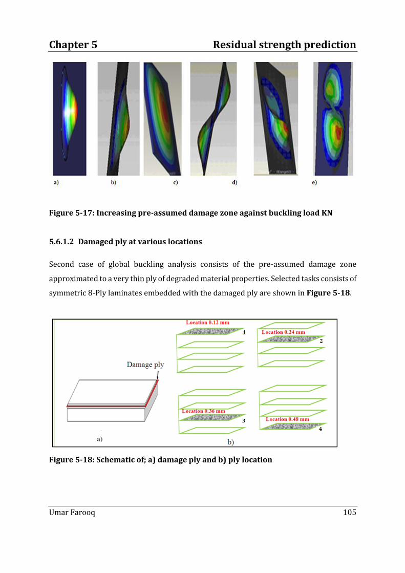
Chapter 5 Residual strength prediction
Umar Farooq 105
Figure 5-17: Increasing pre-assumed damage zone against buckling load KN
5.6.1.2 Damaged ply at various locations
Second case of global buckling analysis consists of the pre-assumed damage zone
approximated to a very thin ply of degraded material properties. Selected tasks consists of
symmetric 8-Ply laminates embedded with the damaged ply are shown in Figure 5-18.
Figure 5-18: Schematic of; a) damage ply and b) ply location

Chapter 5 Residual strength prediction
Umar Farooq 106
Simulations were carried out by moving the damage ply from the top position up to the
middle for global buckling analysis. Position of the damage ply and the buckling loads were
compared against the symmetric and un-symmetric laminates. Comparisons of the buckling
loads against through-the-thickness position of the damaged ply have shown in column
charts of 8-Ply Figure 5-19, 16-Ply laminate in Figure 5-20, and 24 plies Figure 5-21.
Consistent behaviour can be observed in laminates of different lay-ups. Severe load drop
can be seen if pre-assumed damaged ply is located at top, bottom or around the middle
surface. It can be seen that ply locations have minimal effect in regions away from outer
and middle surfaces. The behaviour of a delamination positioned very close to the surface
(and relatively long) at the critical buckling load could be closely affiliated with the
delamination size. The buckling loads increases till mid-surface then start to decrease
around middle plane. The damage ply location has a significant influence, especially on the
buckling mode. It can be seen that the increased delaminated zones have considerable
effects on buckling load. However, a very little effect can be observed if damage ply is
located at or around the middle surface.
Figure 5-19: Buckling load against damage location of ply in 8-Ply laminate

Chapter 5 Residual strength prediction
Umar Farooq 107
Figure 5-20: Buckling load against damage location of ply in 16-Ply laminate
Figure 5-21: Buckling load against damage location of ply in 24-Ply laminate

Chapter 5 Residual strength prediction
Umar Farooq 108
5.6.2 Local buckling analysis
The local buckle is the phenomenon when delaminated plies start buckling at loads lower
than those needed to achieve global buckling. Experimental studies [1] show that the
failure under compression is generally governed by local buckling of the delaminated areas.
Depending on the lay-up thinner of the two outermost plies adjacent to the free surfaces
most likely buckle first. The interior sub-laminates are constrained by the outer sub-
laminates thus could not buckle first. For the case of identical sub-laminates at the top and
bottom surfaces either simultaneous buckling occurs or just one ply buckles first due to
geometric or material defects. Whereas when locally buckling indicated laminates still have
residual strength and do not exhibit catastrophic failures. Two independent cases were
simulated for local buckling:
The 1st case (pre-assumed damage) consists of a hole equivalent to a single ply
thickness located at the central position (75 x 60) of the laminate.
In the 2nd case two parts were assembled: the first part consists of a laminate with a
circular hole; the other part was a circular disk inserted into the vacant hole with
degraded properties to fill the hole.
Simulations were also performed for the increased ply-by-ply damage zones successively
moving locations through-the-thickness. Positions of the pre-assumed damage zone shifted
from top up to the middle surface are shown in schematic view of 8-Ply laminates in Figure
5-22.
Figure 5-22: Symmetric 8-Ply laminate: a) hole and b) damage
X
Y

Chapter 5 Residual strength prediction
Umar Farooq 109
5.6.2.1 Single pre-assumed damaged zone at various locations
Comparisons for buckling load and through-thickness position are also shown in the
column charts for both the simulation cases. Column chart for 24-Ply laminated induced
with delaminated zone diameter: 20 mm in Figure 5-23; 40 mm in Figure 5-24; 60 mm in
Figure 5-25; 80 mm in Figure 5-26; and 100 mm is shown in Figure 5-27. Comparisons of
all the column charts show that difference between holed and degraded cases remains
negligible for first four pre-assumed damage zones. However, significant difference can be
seen in column chart produced for damage zone diameter equal to 100 mm. Column charts
show increasing trend in buckling loads when damaged zones are located towards the mid-
plane in all cases. An increase of delamination zone leads to a decrease in buckling load an
effect which is more pronounced when the delamination is located closer to the outer
surfaces. As damage ply moves further (deep) inside the laminate, the corresponding
buckling load values increase. The delamination location has a significant influence,
especially on the buckling load around outer surfaces.
Figure 5-23: Buckling load against pre-assumed damage diameter: 20 mm
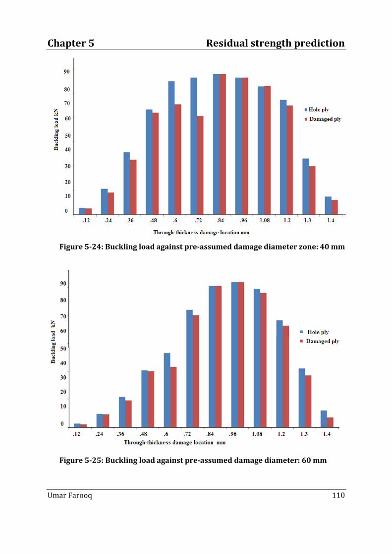
Chapter 5 Residual strength prediction
Umar Farooq 110
Figure 5-24: Buckling load against pre-assumed damage diameter zone: 40 mm
Figure 5-25: Buckling load against pre-assumed damage diameter: 60 mm

Chapter 5 Residual strength prediction
Umar Farooq 111
Figure 5-26: Buckling load against pre-assumed damage diameter: 80 mm
Figure 5-27: Buckling load against pre-assumed damage diameter: 100 mm

Chapter 5 Residual strength prediction
Umar Farooq 112
5.6.2.2 Multiple pre-assumed damaged zone at various locations
Cases of pre-assumed delaminated zones diameter: 20, 40, 60, 80 to 100 mm2 were
simulated at various through-thickness locations from top to bottom for laminate systems.
Simulation produced buckling loads were compared against pre-assumed damage locations
for laminates of 8, 16, and 24 plies in both cases. Selected comparison of the buckling load
values against through-the-thickness position for typical 24 ply laminates is shown in
Figure 5-28 and Figure 5-29. Results produced by simulation of both the cases show
similar trends. Comparisons of multiple delaminated zones show clear difference among
load drops corresponding to damage sizes. Comparison of the values also show significant
effect of the position of the damage ply on the buckling load at or around the top/bottom
most plies.
Figure 5-28: Case 1: Buckling load against multiple damage for 24-Ply laminate

Chapter 5 Residual strength prediction
Umar Farooq 113
Figure 5-29: Case 2: Buckling load against multiple damage for 24-Ply laminate
5.6.2.3 Switching of local and global buckling modes
Simulation produced contour images for both the cases are shown in Figure 5-30, Figure
5-30(a) & (b). Buckling response of a laminate could be very small due to the very weak
natural bending moment. However, under increased loading deflection the neutral axis of
the sub-laminate results in the formation of the ply buckling. The local mode corresponds
to delaminations very close to the surface; is called the open mode to delaminations located
above the critical depth. Relatively deeper delaminations, bending is more significant due
to more substantial natural bending moment. Thus, the larger flexural response of the
laminate effectively produces a larger shift of the neutral axis, and therefore, the global
buckling develops soon after initial buckling. Baker reported in [70] that the response
switches from opened to closed, as the position of the delamination progresses towards the
middle surface. The local mode corresponds to delaminations deeper to delaminations
located above the critical depth is called the closed mode. The trend can be seen in contour
images of mode shapes produced from 0.12 mm to 0.6 mm locations for 24-Ply laminate.

Chapter 5 Residual strength prediction
Umar Farooq 114
Figure 5-30: Local buckling turns to global buckling (damage location effect)
5.7 Mixed-mode buckling simulation
The third case consists of an extension to the global and local buckling cases that include
damage size as well as damaged ply is shown in Figure 5-31. Due to two types of pre-
assumed damages simulations it generates mix-mode buckling which is very complicated to
correlate and segregate. However, similar trends in load drops and damage around the
outer surfaces could be correlated to local buckling modes dominate while global buckling
modes persist in the vicinity of the mid-planes of laminates. Such mixed-mode buckling
modes appear among plies with different orientations and sensitive to impact and
delaminations.

Chapter 5 Residual strength prediction
Umar Farooq 115
Figure 5-31: Schematics of mixed-mode buckling model
Laminates embedded with internal damage make the delamination grow in mixed-mode
after interacting with damaged ply. Generally, critical load increases as depth of the
delamination increases. However, in depths where local buckling is the dominant
mechanism a reversal can be observed as shown in Figure 5-32, Figure 5-33 and Figure
5-34, where load initially decreases and then starts to increase. This phenomenon is
normally observed for larger initial delamination sizes in practice. And the buckling load
increases as damage ply shifts towards the mid-plane before the reverse trend. All curves
show consistent load-drops at and around the vicinity of the middle-plane of the laminate.
This behaviour indicates mixed-mode buckling when damage zone and damage ply are
located together around the middle surface. The turning points on the curves indicate a
threshold condition where the failure mechanism of the laminate alters. Before the turning
point the entire laminate fails due to the snap-through buckling. An increased local buckling
at and around the outer surface could result in severe instabilities and catastrophic failures
far below the allowable limits. However, damage ply location leads to an increased buckling
load when the ply is located closer to the mid-surface. Snap-through, mixing-mode or global
buckling may occur depending on the particular values of the delamination size and
coupling interaction with ply location. Laminate’s ability to resist compressive loads and
behave as a more damage tolerant structure greatly depends on through-the-thickness
location of the damage zone and damaged ply.
X
Y
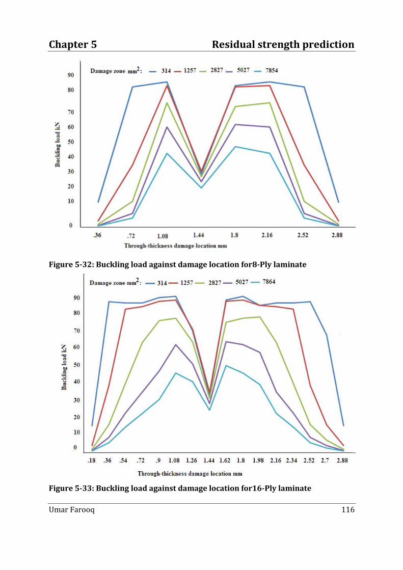
Chapter 5 Residual strength prediction
Umar Farooq 116
Figure 5-32: Buckling load against damage location for8-Ply laminate
Figure 5-33: Buckling load against damage location for16-Ply laminate
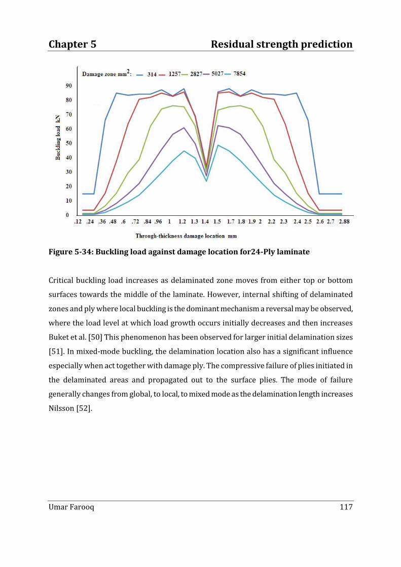
Chapter 5 Residual strength prediction
Umar Farooq 117
Figure 5-34: Buckling load against damage location for24-Ply laminate
Critical buckling load increases as delaminated zone moves from either top or bottom
surfaces towards the middle of the laminate. However, internal shifting of delaminated
zones and ply where local buckling is the dominant mechanism a reversal may be observed,
where the load level at which load growth occurs initially decreases and then increases
Buket et al. [50] This phenomenon has been observed for larger initial delamination sizes
[51]. In mixed-mode buckling, the delamination location also has a significant influence
especially when act together with damage ply. The compressive failure of plies initiated in
the delaminated areas and propagated out to the surface plies. The mode of failure
generally changes from global, to local, to mixed mode as the delamination length increases
Nilsson [52].

Chapter 5 Residual strength prediction
Umar Farooq 118
5.8 Summary
Pre-assumed delamination zone corresponding to gross damage zones were induced within
the laminates. Various tasks for global, local, and mixed-mode buckling were performed to
accomplish correlation of the anticipated range of delamination zones against predicted
residual strength. Simulation produced bucking loads and buckling modes were correlated
to the delamination size, delamination zone/ply depths, and coupled effects. Comparison
and correlation of the simulation produced results against theoretically, experimentally and
intra-simulation data available in the literature and found to be within acceptable
agreement.
Results show that the buckling load decreases as the delamination size increases, especially
when the delamination spread across the entire length of the laminate at the beginning in
local and at the end in global buckling mode. Moreover, residual load carrying capacity
approached to the critical buckling load where single mode split in two opposite modes at
larger delaminations. Deeper-located larger delaminations produced failure due to global
buckling. The buckled sub-laminates (segments) were found responsible for the structural
instability. The local buckling mode evolved as global buckling mode configuration at the
deeper position and depth of the delaminations resulting failure or degradation of the
laminate due to shear rigidity/mode. Results from the mixed-mode buckling correlated to
the pre-assumed delaminated zone where damage zone and damaged ply show severe load
drop at outer surfaces and snap-shot failure around mid-surfaces.

Chapter 5 Residual strength prediction
Umar Farooq 119

Chapter 6 Determination of properties
Umar Farooq 120
Chapter 6 Determination of physical and mechanical properties
6.1 Review
This chapter is concerned with determining physical and mechanical properties of fibre
reinforced laminated composite materials. Two types of materials were characterized. The
data relating to the first type of material of code IM7/8552 infused with epoxy-resin matrix
properties was previously determined by [1]. Properties of laminates consisting of code
Fibre dux 914C-833-40 were determined. The code is defined below:
Designation-914-175C Degree cured resin which when post cured at 190C Degrees gives a
continuous operating temperature capability of 125 C Degrees.
-C -Carbon Fibre (Torayca T300)
-833 -5 Harness Satin Woven Carbon Fibre Fabric
-40 -Percentage of Resin contents by weight.
Physical properties were determined from ignition loss tests. Micro-macro mechanics
relations were applied to determine the engineering constants. Theoretical formulations
were extended to approximate full range of engineering constants for lamina, laminate, and
structural elements. Tensile and flexural tests were conducted to determine in-plane elastic
constants in line with the standards procedures using universal test model INSTRONTM
5585H.
Theoretically and experimentally determined values were compared and validated.
6.2 Determination of properties
Most of the structural parts use laminates that consist of several plies with different carbon
fibre orientations connected together through a bonding interface. Composites are
heterogeneous materials hence full characterisation of their properties is difficult as
various processing factors can influence the properties such as misaligned fibres, fibre
damage, non-uniform curing, cracks, voids and residual stresses. These factors are assumed
negligible when care is taken in the manufacturing process. It is for this reason that the
purpose specific aerospace specialist fabricated laminates (manufacturers’ supplied) were

Chapter 6 Determination of properties
Umar Farooq 121
used here. The constituents are also assumed to be void- free, linear elastic. The process of
determining physical and mechanical properties of a fibrous composite laminate is outlined
in a flowchart shown below in Figure 6-1.
Figure 6-1: Flowchart of determining physical and mechanical properties
6.3 Determination of physical properties
The types of laminates consisting of code Fibredux 914C-833-40 embedded with fibre
horns technique of every forth layer. Average thicknesses of the laminates consisting of 8-,
16-, and 34-Ply sequence are given in with error margins Table 6-1.

Chapter 6 Determination of properties
Umar Farooq 122
Table 6-1: Measured geometrical properties
Laminates Fibredux 914C-833-40
No of ply Average thickness mm Error margin ± mm
8 2.4 0.198
16 4.8 0.023
24 7.2 0.026
Fibre content of resin–matrix and densities were determined experimentally determined
by the ignition loss method experimentally determined by the ignition loss method (ASTM:
D2854-68). The ignition loss method is used for polymeric matrix composites containing
fibres that do not lose weight at high temperature. In this method, cured resin is burned off
from a small test at 5850C in a muffle furnace. After the burning for three hours at 585 0C
density of fibres comes down to 1.8 g/cm3 and that of the matrix as 2.09 g/cm3. Three
laminates were tested and fibre percentage (residue mass/sample mass) per unit volume
(cm3) is shown in Table 6-2 given below.
Table 6-2: Fibre contents of laminate of code Fibredux 914c-833-40.
Sample Heated up to 585 0C
Length Width Depth Sample
mass g
Residue
mass g
Density
g/cm3
Carbon fibre %
A 22.40 2.13 5.89 0.4434 0.17 1.779 45.37
B 13.4 5.84 11.56 1.4555 0.7396 1.816 50.8
C 12.61 5.75 11.47 1.3924 0.7027 1.786 50.5
6.4 Determination of elastic properties of a lamina (Rule of Mixture)
A lamina forms the building block of composite laminates and structures. The mechanical
and physical properties of a lamia are (reinforcement and matrix) and their interaction is
examined on a microscopic level. Rules of mixture expresses the micromechanics laws in a
predictable form based on various degree of simplifications. Fibre and composite densities

Chapter 6 Determination of properties
Umar Farooq 123
are measured and then converted into fibre volume fraction using the standard formulae.
The volume fractions form basis for approximation of engineering properties the material.
Volume of a laminate can be related to its ingredients using ‘rule of mixture’:
𝑽𝒄 = 𝑽𝒇 + 𝑽𝒎 + 𝑽𝒗 (6-1)
Assumption negligible voids:
𝑾𝒄
𝝆𝒄=
𝑾𝒇
𝝆𝒇+
𝑾𝒄−𝑾𝒇
𝝆𝒎 (6-2)
𝟏 =
𝑾𝒇
𝝆𝒇 +
𝑾𝒄−𝑾𝒇
𝝆𝒎
𝑾𝒄𝝆𝒄
(6-3)
𝑽𝒄 = 𝟏 −
𝑾𝒇
𝝆𝒇 +
𝑾𝒄−𝑾𝒇
𝝆𝒎
𝑾𝒄𝝆𝒄
(6-4)
Where: The symbols W, V, and ρ represent weight, volume, and density. The subscripts c, f,
m, and v denote composite, fibre, matrix, and void, respectively. Density of a composite can
be express by Eq. (6-5):
𝝆𝒄 = 𝝆𝒇𝑽𝒇 + 𝝆𝒎𝑽𝒎 (6-5)
Fibre volume fraction from densities neglecting void contents zero is:
𝑭𝑽𝑭 = 𝝆𝒄−𝝆𝒎
𝝆𝒇−𝝆𝒎 (6-6)
The fibre volume fraction from fibre weight fraction
𝑭𝑽𝑭 = 𝟏 +𝝆𝑭
𝝆𝒎
𝟏
𝑭𝑾𝑭− 𝟏
−𝟏
(6-7)
Where
𝑭𝑾𝑭 =𝝆𝑭𝒙𝑭𝑽𝑭
𝝆𝒎+ 𝝆𝒇−𝝆𝒎 .𝑭𝑽𝑭 (6-8)
The cured ply thickness from ply weight
𝑪𝑷𝑻 𝒎𝒎 =𝑾𝑭
𝟏𝟎𝟎𝟎 𝝆𝒇𝑭𝑽𝑭 (6-9)
Fibre volume fraction using Esq. (6-7) and Esq. (6-8) can be re-written as:
𝑽𝒇 =𝑾𝒇
𝝆𝒇
𝑾𝒇
𝝆𝒇+ (1 − 𝑾𝒇 𝝆𝒎
−1
(6-10)
𝝆𝒄 = 𝟏𝒙 𝑾𝒇
𝝆𝒇+ (1 − 𝑾𝒇 𝝆𝒎
−1
(6-11)

Chapter 6 Determination of properties
Umar Farooq 124
In terms of fibre volume fraction,𝑽𝒇, the composite density, 𝝆𝒄, can be written as
𝝆𝒄 = 𝝆𝒇𝑽𝒇 + 𝝆𝒎 𝟏 − 𝝆𝒇 (6-12)
From the assumption of perfect bonding between fibres and matrix, we can write:
𝑬𝒇 = 𝑬𝒎 = 𝐸𝒄 (6-13)
Since both fibres and matrix are elastic, the representative longitudinal systems can be
calculated as
𝝇𝒇 = 𝑬𝒇𝜺𝒇 = 𝑬𝒇𝜺𝑐 (6-14)
𝝇𝒎 = 𝑬𝒎𝜺𝒎 = 𝑬𝑚𝜺𝑐 (6-15)
Comparing Eq. (6-14) and Eq. (6-15) and from material properties that 𝐸𝑓 ≫ 𝐸𝑚 we
conclude that the fibre stress 𝜍𝑓 is always greater than the 𝜍𝑚 . The total tensile load P
applied on the composite lamina is shared by fibres and matrix so that
𝑷 = 𝑷𝒇 + 𝑷𝒎 (6-16)
Equation (7-16) can be written as
𝝇𝒄𝑨𝑐 = 𝝇𝒇𝑨𝑓 + 𝝇𝒎𝑨𝑚 (6-17)
or
𝝇𝒄 = 𝝇𝒇𝑨𝑓
𝑨𝑐+ 𝝇𝒎
𝑨𝑚
𝑨𝑐 (6-18)
Since 𝑽𝒇 =𝑨𝑓
𝑨𝑐 and 𝑽𝒎 =
𝑨𝑚
𝑨𝑐, the Eq. (7-18) gives
𝝇𝒄 = 𝝇𝒇𝑽𝒇 + 𝝇𝒎𝑽𝒎 (6-19)
=𝝇𝒇𝑽𝒇 + 𝝇𝒎 1 − 𝑽𝒇 (6-20)
Dividing both sides of the Eq. (6-20) by 휀𝑐 and using Eqs. (6-14) & (6-15), we can write the
longitudinal modulus for the composites as
𝑬𝐿 = 𝑬𝒇𝑽𝒇 + 𝑬𝑚 1 − 𝑽𝒇 (6-21)
Equation (7-21) is called the rule of mixture that shows that the composite’s longitudinal
modulus is intermediate between fibre and matrix moduli. The fraction of load carried by
fibres in a unidirectional continuous fibre lamina is
𝑷𝑓
𝑃= 𝝇𝒇𝑽𝒇 𝝇𝒇𝑽𝒇 + 𝝇𝒎 1 − 𝑽𝒇
−1
= 𝑬𝒇𝑽𝒇 𝑬𝒇𝑽𝒇 + 𝑬𝒎 1 − 𝑽𝒇 −1
(6-22)

Chapter 6 Determination of properties
Umar Farooq 125
In polymeric matrix composites, 𝑬𝑓
𝐸𝑚> 10. Thus, even for 𝑽𝒇 = 0.2, fibres carry more than
70% of composite load. In general, the fibre failure strain is lower than the matrix failure
strain. Assuming all fibres have the same strength, the tensile rupture of fibre will
precipitate a tensile rupture in the composites. Thus, using Eq. (6-20), the longitudinal
tensile strength 𝜍𝐿𝑡𝑢 of a unidirectional continuous fibre can be estimated as
𝝇𝑳𝒕𝒖 = 𝝇𝒇𝒖 + 𝝇𝒎𝒖𝒔 1 − 𝑽𝒇 (6-23)
Where: 𝜍𝑓𝑢 is fibre tensile strength; 𝜍𝑚𝑢𝑠 is matrix stress (휀𝑚 = 휀𝑓𝑢 ).
For effective measurement of the reinforcement of the matrix for 𝝇𝑳𝒕𝒖 ≥ 𝝇𝒎𝒖 the fibre
volume fraction in the composite must be greater than a critical value. This critical volume
fraction is calculated by setting 𝝇𝑳𝒕𝒖 = 𝝇𝒎𝒖. Thus, from Eq. (6-23), the value can be
calculated as:
𝑽𝒇_𝑪𝒓𝒊𝒕𝒊𝒄𝒂𝒍 = 𝝇𝒎𝒖 − 𝝇𝒎𝒖𝒔 𝝇𝒇𝒖 − 𝝇𝒎𝒖𝒔 −1
(6-24)
From the Eq. (6-24) fibre volume fraction was determined as 54%. The acceptable range of
(±5%) fibre contents lead to determine elastic constants to verify (the major requirement)
before using in the investigation. Engineering constants for unidirectional lamina enforced
with continuous fibre aligned in x direction can be calculated from the following equations:
𝑬11 = 𝑬𝒇𝑽𝒇 + 𝑬𝑚𝑽𝒎 (6-25)
𝝂11 = 𝜈𝒇𝑽𝒇 + 𝝂𝑚𝑽𝒎 (6-26)
𝑬22 = 𝑬𝒇𝑬𝒎
𝑬𝒇𝑽𝒎+𝑬𝒎𝑽𝒇 (6-27)
𝝂𝟐𝟏 = 𝑬𝟐𝟐
𝑬𝟏𝟏𝝂𝟏𝟐 (6-28)
𝐆12 = 𝑮𝒇𝑮𝑚
𝑮𝒇𝑽𝑚 +𝑮𝑚 𝑽𝑓 (6-29)
The engineering constants (E1, E2, G12 and v12) computed through the ‘Rules of Mixture’ at
micromechanics level can be utilised to examine response on a macroscopic scale as shown
in Figure 2-1 up to failure and residual properties of laminates. Utilising the engineering
constants the following equations are used to calculate the elastic properties of an angle-ply

Chapter 6 Determination of properties
Umar Farooq 126
lamina in which continuous fibres are aligned at angle 𝜃 as shown in Figure 3-3 with
positive x direction:
𝟏
𝑬𝒙𝒙=
𝒄𝒐𝒔𝟒𝜽
𝑬𝟏𝟏+
𝒔𝒊𝒏𝟒𝜽
𝑬𝟐𝟐+
𝟏
𝟒
𝟏
𝑮𝟏𝟐− 𝟐
𝝂𝟏𝟐
𝑬𝟏𝟏 𝒔𝒊𝒏𝟐𝟐𝜽 (6-30)
𝟏
𝑬𝒚𝒚=
𝒔𝒊𝒏𝟒𝜽
𝑬𝟏𝟏+
𝒄𝒐𝒔𝟒𝜽
𝑬𝟐𝟐+
𝟏
𝟒
𝟏
𝑮𝟏𝟐− 𝟐
𝝂𝟏𝟐
𝑬𝟏𝟏 𝒔𝒊𝒏𝟐𝟐𝜽 (6-31)
𝟏
𝑮𝒙𝒚=
𝟏
𝑬𝟏𝟏+
𝟐𝝂𝟏𝟐
𝑬𝟏𝟏+
𝟏
𝑬𝟐𝟐−
𝟏
𝑬𝟏𝟏+
𝟐𝝂𝟏𝟐
𝑬𝟏𝟏+
𝟏
𝑬𝟐𝟐−
𝟏
𝑮𝟏𝟐 𝒄𝒐𝒔𝟐𝟐𝜽 (6-32)
𝝂𝒙𝒚 = 𝑬𝒙𝒙 𝝂𝟏𝟐
𝑬𝟏𝟏−
𝟏
𝟒
𝟏
𝑬𝟏𝟏+
𝟐𝝂𝟏𝟐
𝑬𝟏𝟏+
𝟏
𝑬𝟐𝟐−
𝟏
𝑮𝟏𝟐 𝑠𝑖𝑛22𝜃 (6-33)
𝝂𝒚𝒙 =𝑬𝒚𝒚
𝑬𝒙𝒙𝝂𝒙𝒚 (6-34)
6.5 Engineering constants for orthotropic lamina in 2D
For a thin isotropic lamina in a plane stress (𝜍𝑧𝑧 = 𝜏𝑥𝑧 = 𝜏𝑦𝑧 = 0) the stress-strain relations
as shown in Figure 6-2 in the elastic range are
Figure 6-2: Stresses in an isotropic lamina under a plane stress condition.
𝜺𝒙𝒙 =𝟏
𝑬 𝝇𝒙𝒙 − 𝝊𝝇𝒚𝒚
𝜺𝒚𝒚 =𝟏
𝑬 −𝝊𝝇𝒙𝒙 + 𝝇𝒚𝒚

Chapter 6 Determination of properties
Umar Farooq 127
𝜸𝒙𝒚 =𝟏
𝑮 𝝉𝒙𝒚 (6-35)
There is no coupling between the shear stresses and normal stress. However, orthotropic
lamina in a plane stress, stress-strain relations as shown Figure 6-3 in the elastic range
are:
𝜺𝒙𝒙 =𝝇𝒙𝒙
𝑬𝒙𝒙− 𝝊𝒚𝒙
𝝇𝒚𝒚
𝑬𝒚𝒚− 𝒎𝒙𝝉𝒙𝒚
𝜺𝒚𝒚 = −𝝊𝒙𝒚𝝇𝒙𝒙
𝑬𝒙𝒙+
𝝇𝒚𝒚
𝑬𝒚𝒚− 𝒎𝒚𝝉𝒙𝒚
𝜸𝒙𝒚 = −𝒎𝒙𝝇𝒙𝒙 − 𝒎𝒚𝝇𝒚𝒚 +𝝉𝒙𝒚
𝑮𝒙𝒚 (6-36)
Figure 6-3: Orthotropic lamina in a plane stress
Stresses in a general orthotropic lamina under a plane stress conditions
Where 𝐸𝑥𝑥 𝐸𝑦𝑦 𝜐𝑥𝑦 and 𝜐𝑦𝑥 are elastic constants for the lamina obtained from angle-lamina
equations and 𝑚𝑥 and 𝑚𝑦 are given by the following equations:
𝒎𝒙 = 𝒔𝒊𝒏𝟐𝜽 𝝂𝟏𝟐
𝑬𝟏𝟏+
𝟏
𝑬𝟐𝟐−
𝟏
𝟐𝑮𝟏𝟐− 𝒄𝒐𝒔𝟐𝜽
𝟏
𝑬𝟏𝟏+
𝟐𝝂𝟏𝟐
𝑬𝟏𝟏+
𝟏
𝑬𝟐𝟐−
𝟏
𝑮𝟏𝟐 (6-37)
𝒎𝒚 = 𝒔𝒊𝒏𝟐𝜽 𝝂𝟏𝟐
𝑬𝟏𝟏+
𝟏
𝑬𝟐𝟐−
𝟏
𝟐𝑮𝟏𝟐− 𝒔𝒊𝒏𝟐𝜽
𝟏
𝑬𝟏𝟏+
𝟐𝝂𝟏𝟐
𝑬𝟏𝟏+
𝟏
𝑬𝟐𝟐−
𝟏
𝑮𝟏𝟐 (6-38)

Chapter 6 Determination of properties
Umar Farooq 128
The new constants 𝑚𝑥 and 𝑚𝑦 represent the influence of shear stresses on extensional
strains in Eqs (6-34) and (6-35) and the influence of normal stresses on shear strains in Eq.
(6-36). These constants are called coefficients of mutual influence. Observations can be
made from Eq. (6-34) into Eq. (6-38). For an especially orthotropic lamina, the stress-strain
relations produced in Chapter 3 may be re-written as:
𝜺𝒙𝒙 = 𝜺𝟏𝟏 =𝝇𝒙𝒙
𝑬𝟏𝟏− 𝝊𝟐𝟏
𝝇𝒚𝒚
𝑬𝟐𝟐
𝜺𝒚𝒚 = 𝜺𝟐𝟐 = −𝝊𝟏𝟐𝝇𝒙𝒙
𝑬𝟏𝟏+
𝝇𝒚𝒚
𝑬𝟐𝟐
𝜸𝒙𝒚 = 𝜸𝒚𝒙 = 𝜸𝟏𝟐 = 𝜸𝟐𝟏𝝉𝒙𝒚
𝑮𝒙𝒚 (6-39)
Both 𝑚𝑥 and 𝑚𝑦 are functions of orientation angle 𝜃 only and exhibit maximum values at an
intermediate angle between 𝜃 = 0 a𝑛𝑑 90. The stiffness matrices for isotropic lamina 𝑄 is
equal to inverse of the compliance matrix 𝑄 −1. For Specially orthotropic lamina
(𝜃 = 0 𝑎𝑛𝑑 90) the stress-strain relations becomes
𝝇𝟏
𝝇𝟐
𝝉𝟏𝟐
= 𝑸𝟏𝟏 𝑸𝟏𝟐 𝟎𝑸𝟏𝟐 𝑸𝟐𝟐 𝟎𝟎 𝟎 𝑸𝟔𝟔
𝜺𝟏
𝜺𝟐𝜸𝟏𝟐
𝟐
(6-40)
Where the Qij are the components of the lamina stiffness matrix:
𝑸𝟏𝟏 =𝑺𝟐𝟐
𝑺𝟏𝟏𝑺𝟐𝟐−𝑺𝟏𝟐𝟐 =
𝑬𝟏
𝟏−𝝊𝟏𝟐𝝊𝟐𝟏
𝑸𝟏𝟐 = −𝑺𝟏𝟐
𝑺𝟏𝟏𝑺𝟐𝟐−𝑺𝟏𝟐𝟐 =
𝝊𝟏𝟐𝑬𝟐
𝟏−𝝊𝟏𝟐𝝊𝟐𝟏= 𝑸𝟐𝟏
𝑸𝟐𝟐 =𝑺𝟏𝟏
𝑺𝟏𝟏𝑺𝟐𝟐−𝑺𝟏𝟐𝟐 =
𝑬𝟐
𝟏−𝝊𝟏𝟐𝝊𝟐𝟏
𝑸𝟔𝟔 =𝟏
𝑺𝟔𝟔= 𝑮𝟏𝟐
While the compliance coefficients can be obtained as:
𝑺𝟏𝟏 = 𝟏
𝑬𝟏, 𝑺𝟐𝟐 =
𝟏
𝑬𝟐, 𝑺𝟏𝟐 = 𝑺𝟐𝟏 =
−𝝊𝟐𝟏
𝑬𝟐=
−𝝊𝟏𝟐
𝑬𝟏, 𝑺𝟔𝟔 =
𝟏
𝑮𝟏𝟐.
Similarly, for the general orthotropic lamina (𝜃 ≠ 0 𝑎𝑛𝑑 90), the complete set of
transformation equations for the stresses in the xy-coordinate system can be developed
using the transformation matrix
𝝇𝟏
𝝇𝟐
𝝉𝟏𝟐
= 𝑻
𝝇𝒙
𝝇𝒚
𝝉𝒙𝒚
(6-41)

Chapter 6 Determination of properties
Umar Farooq 129
Where 𝑇 = 𝑚2 𝑛2 2𝑚𝑛𝑛2 𝑚2 −2𝑚𝑛
−𝑚𝑛 𝑚𝑛 𝑚2 − 𝑛2
and 𝑚 = 𝑐𝑜𝑠 𝜃 𝑎𝑛𝑑 𝑛 = 𝑠𝑖𝑛 𝜃
For the generally orthotropic laminate carrying out the matrix multiplication and
converting back to engineering strains, we find from the reduced transformed stiffness
matrix.
𝝇𝒙
𝛔𝒚
𝝉𝒙𝒚
=
𝑸 𝟏𝟏 𝑸 𝟏𝟐 𝑸 𝟏𝟔
𝑸 𝟏𝟐 𝑸 𝟐𝟐 𝑸 𝟐𝟔
𝑸 𝟏𝟔 𝑸 𝟐𝟔 𝑸 𝟔𝟔
𝜺𝒙
𝜺𝒚
𝜸𝒙𝒚
(6-42)
Where the 𝑄 𝑖𝑗 are the components of the transformed lamina stiffness matrix which are
defined as follows:
𝑸 𝟏𝟏 = 𝑸𝟏𝟏𝒄𝒐𝒔𝟒𝜽 + 𝑸𝟐𝟐𝒔𝒊𝒏𝟒𝜽 + 𝟐 𝑸𝟏𝟐 + 𝟐𝑸𝟔𝟔 𝒔𝒊𝒏
𝟐𝜽𝒄𝒐𝒔𝟐𝜽
𝑸 𝟏𝟐 = 𝑸𝟏𝟏 + 𝑸𝟐𝟐 − 𝟒𝑸𝟔𝟔 𝒔𝒊𝒏𝟐𝜽𝒄𝒐𝒔𝟐𝜽 + 𝑸𝟏𝟐 𝒄𝒐𝒔𝟒𝜽 + 𝒔𝒊𝒏𝟒𝜽
𝑸 𝟐𝟐 = 𝑸𝟏𝟏𝐜𝒐𝒔𝟒𝜽 + 𝑸𝟐𝟐𝒔𝒊𝒏𝟒𝜽 + 𝟐 𝑸𝟏𝟐 + 𝟐𝑸𝟔𝟔 𝒔𝒊𝒏
𝟐𝜽𝒄𝒐𝒔𝟐𝜽
𝑸 𝟏𝟔 = 𝑸𝟏𝟏 − 𝑸𝟏𝟐 − 𝟐𝑸𝟔𝟔 𝒔𝒊𝒏𝜽 𝒄𝒐𝒔𝟑𝜽 − 𝑸𝟐𝟐 − 𝑸𝟏𝟐 − 𝟐𝑸𝟔𝟔 𝒄𝒐𝒔𝜽 𝒔𝒊𝒏𝟑𝜽
𝑸 𝟐𝟔 = 𝑸𝟏𝟏 − 𝑸𝟏𝟐 − 𝟐𝑸𝟔𝟔 𝒄𝒐𝒔𝜽 𝒔𝒊𝒏𝟑𝜽 − 𝑸𝟐𝟐 − 𝑸𝟏𝟐 − 𝟐𝑸𝟔𝟔 𝒔𝒊𝒏𝜽 𝒄𝒐𝒔𝟑𝜽
𝑸 𝟔𝟔 = 𝑸𝟏𝟏 + 𝑸𝟐𝟐 − 𝟐𝑸𝟏𝟐 − 𝟐𝑸𝟔𝟔 𝒔𝒊𝒏𝟐𝜽𝒄𝒐𝒔𝟐𝜽 + 𝑸𝟔𝟔 𝒄𝒐𝒔𝟒𝜽 + 𝒔𝒊𝒏𝟒𝜽 (6-43)
From Eq. (6-42) it appears that there are six elastic constants that govern the stress-strain
behaviour of a lamina. However, these equations are linear combinations of the four basic
elastic constants, and therefore are not independent. Elements in stiffness and compliance
matrices can be expresses in terms of five invariant properties of the lamina. Using
trigonometric identities have shown that the elements in stiffness matrix can be written as
𝑸 𝟏𝟏 = 𝑼𝟏 + 𝑼𝟐𝒄𝒐𝒔𝟐𝜽 + 𝑼𝟑𝒄𝒐𝒔𝟒𝜽
𝑸 𝟏𝟐 = 𝑼𝟒 − 𝑼𝟑𝒄𝒐𝒔𝟒𝜽
𝑸 𝟐𝟐 = 𝑼𝟏 − 𝑼𝟐𝒄𝒐𝒔𝟐𝜽 + 𝑼𝟑𝒄𝒐𝒔𝟒𝜽
𝑸 𝟏𝟔 = 𝑼𝟐
𝟐𝒔𝒊𝒏𝟐𝜽 + 𝑼𝟑𝒔𝒊𝒏𝟒𝜽
𝑸 𝟐𝟔 = 𝑼𝟐
𝟐𝒔𝒊𝒏𝟐𝜽 − 𝑼𝟑𝒔𝒊𝒏𝟒𝜽
𝑸 𝟔𝟔 = 𝟏
𝟐 𝑼𝟏 − 𝑼𝟒 − 𝑼𝟑 𝒄𝒐𝒔 𝟒𝜽 (6-44)

Chapter 6 Determination of properties
Umar Farooq 130
Where the set of invariants is defined as
𝑼𝟏 =𝟏
𝟖 𝟑𝑸𝟏𝟏 + 𝟑𝑸𝟐𝟐 + 𝟐𝑸𝟏𝟐 + 𝟒𝑸𝟔𝟔
𝑼𝟐 =𝟏
𝟐 𝑸𝟏𝟏 − 𝑸𝟐𝟐
𝑼𝟑 =𝟏
𝟖 𝑸𝟏𝟏 + 𝑸𝟐𝟐 − 𝟐𝑸𝟏𝟐 − 𝟒𝑸𝟔𝟔
𝑼𝟒 =𝟏
𝟖 𝟑𝑸𝟏𝟏 + 𝟑𝑸𝟐𝟐 + 𝟔𝑸𝟏𝟐 − 𝟒𝑸𝟔𝟔 (6-45)
The invariants are simply linear combinations of the Qij, are invariant to rotations in the
plane of the lamina. There are four independent invariants, just as there are four
independent elastic constants. Equations (6-44) are obviously easier to manipulate and
interpret then Eq. (6-36). All the stiffness expressions except those for the coupling
stiffness consist of one constant term and terms which vary with lamina orientations. Thus,
the effects of lamina orientation on stiffness are easier to interpret. Similarly, invariant
formulations of lamina compliance transformations can also be written. These invariant
forms are very useful in computing elements of these matrices. The element of fibre-
reinforced composite material with its fibre oriented at some arbitrary angle exhibits a
shear strain when subjected to a normal stress, and it also exhibits an extensional strain
when subjected to a shear stress. The state of stress is defined as 𝜍𝑥𝑥 ≠ 0, 𝜍𝑦𝑦 = 𝜏𝑥𝑦 =
0, the ratio
𝜼𝒙,𝒙𝒚 =𝜸𝒙𝒚
𝛆𝒙𝒙=
𝑺 𝟏𝟔
𝑺 𝟏𝟏 (6-46)
Similarly, when the state of stress is defined as 𝜍𝑦𝑦 ≠ 0, 𝜍𝑥𝑥 = 𝜏𝑥𝑦 = 0, the ratio
𝜼𝒚,𝒙𝒚 =𝜸𝒙𝒚
𝜺𝒚𝒚=
𝑺 𝟐𝟔
𝑺 𝟐𝟐 (6-47)
A pure shear stress 𝜏𝑥𝑦 ≠ 0, 𝜍𝑥𝑥 = 𝜍𝑦𝑦 = 0, the ratio 𝜂𝑥𝑦 ,𝑦 characterises the normal strain
response along the y direction due to a shear stress in the x-y plane. The ratio can be found
as:
𝜼𝒙𝒚,𝒚 =𝜏𝑥𝑦
𝑺 𝟔𝟔 (6-48)
Superposition of loading, stress-strain relations in terms of engineering constants are:

Chapter 6 Determination of properties
Umar Farooq 131
𝜺𝒙𝒙
𝜺𝒚𝒚
𝜸𝒔
=
𝟏
𝑬𝒙𝒙−
𝝂𝒚𝒙
𝑬𝒚𝒚
𝜼𝒔𝒙
𝑮𝒙𝒚
−𝝂𝒚𝒙
𝑬𝒙𝒙
𝟏
𝑬𝒚𝒚
𝜼𝒔𝒚
𝑮𝒙𝒚
𝜼𝒔𝒙
𝑮𝒙𝒚
𝜼𝒔𝒚
𝑮𝒙𝒚
𝟏
𝑮𝒙𝒚
𝝇𝒙𝒙
𝝇𝒚𝒚
𝝉𝒔
(6-49)
The transformation relations yield engineering constants:
𝑬𝒙𝒙 = 𝟏 𝒎𝟐
𝑬𝟏𝟏 𝒎𝟐 − 𝒏𝟐𝝂𝟏𝟐 +
𝒏𝟐
𝑬𝟐𝟐 𝒏𝟐 − 𝒎𝟐𝝂𝟏𝟐 +
𝒎𝟐𝒏𝟐
𝑮𝟏𝟐 (6-50)
𝑬𝒚𝒚 = 𝟏
𝒏𝟐
𝑬𝟏𝟏 𝒏𝟐 − 𝒎𝟐𝝂𝟏𝟐 +
𝒎𝟐
𝑬𝟐𝟐 𝒎𝟐 − 𝒏𝟐𝝂𝟐𝟏 +
𝒎𝟐𝒏𝟐
𝑮𝟏𝟐 (6-51)
𝑮𝒙𝒚 = 𝟏
𝟒𝒎𝟐𝒏𝟐
𝑬𝟏𝟏 𝟏 + 𝝂𝟏𝟐 +
𝟒𝒎𝟐𝒏𝟐
𝑬𝟐𝟐 𝟏 + 𝝂𝟐𝟏 +
𝒎𝟐−𝒏𝟐 𝟐
𝑮𝟏𝟐 (6-52)
𝝂𝒙𝒚 =𝑬𝒙𝒙
𝒎𝟐
𝑬𝟏𝟏 𝒎𝟐𝝂𝟏𝟐 − 𝒏𝟐 +
𝒏𝟐
𝑬𝟐𝟐 𝒏𝟐𝝂𝟏𝟐 − 𝒎𝟐 +
𝒎𝟐𝒏𝟐
𝑮𝟏𝟐
(6-53)
𝝂𝒚𝒙 =𝑬𝒚𝒚𝝂𝒙𝒚
𝑬𝒙𝒙 (6-54)
𝜼𝒙𝒔𝑬𝒙𝒙
=𝜼𝒔𝒙
𝑮𝒙𝒚 =
𝟐𝒎𝟑𝒏
𝑬𝟏𝟏 𝟏 + 𝝂𝟏𝟐 −
𝟐𝒎𝒏𝟑
𝑬𝟐𝟐 𝟏 + 𝝂𝟐𝟏 −
𝒎𝒏 𝒎𝟐−𝒏𝟐
𝑮𝟏𝟐 (6-55)
𝜼𝒚𝒔
𝑬𝒚𝒚 =
𝜼𝒔𝒚
𝑮𝒙𝒚 =
𝟐𝒎𝒏𝟑
𝑬𝟏𝟏 𝟏 + 𝝂𝟏𝟐 −
𝟐𝒏𝒎𝟑
𝑬𝟐𝟐 𝟏 + 𝝂𝟐𝟏 +
𝒎𝒏 𝒎𝟐−𝒏𝟐
𝑮𝟏𝟐 (6-56)
6.6 Engineering constants in 3D
Real structural elements involve lay-ups containing various number of angle plies, of
composite involve thick components subjected to three-dimensional states of stress. The
quadratic mid-plane of the laminate contains the xy-axes, and the z-axis defines the
thickness direction. The total thickness of the laminate is h and the thickness of the
individual lamina is represented by t. Equations (3-1) to (3-9) produced in Chapter 3 can
be re-produced to include un-uniform thickness of ply for the total number of laminas N.
As laminate strains are linearly related to the distance from the mid-plane:
𝜺𝒙𝒙 = 𝜺𝒙𝒙𝟎 + 𝒛𝒌𝒙𝒙

Chapter 6 Determination of properties
Umar Farooq 132
𝜺𝒚𝒚 = 𝜺𝒚𝒚𝟎 + 𝒛𝒌𝒚𝒚
𝜸𝒙𝒚 = 𝜸𝒙𝒚𝟎 + 𝟐𝒛𝒌𝒙𝒚 (6-57)
Where:
휀𝑥𝑥0 , 휀𝑦𝑦
0 = mid-plane normal strains in the laminate
𝛾𝑥𝑦0 = mid-plane shear strain in the laminate
𝑘𝑥𝑥 𝑘𝑦𝑦 = bending curvatures in the laminate
𝑘𝑥𝑦 = twisting curvature in the laminate
𝑧 = distance from the mid-plane in the thickness direction.
The mid-surface and curvature are always zero and not function of z. Integrations at mid-
surface gives:
𝑵𝒙𝒙
𝑵𝒚𝒚
𝑵𝒙𝒚
=
𝑸 𝟏𝟏 𝑸 𝟏𝟐 𝑸 𝟏𝟔
𝑸 𝟏𝟐 𝑸 𝟐𝟐 𝑸 𝟐𝟔
𝑸 𝟏𝟔 𝑸 𝟐𝟔 𝑸 𝟔𝟔
𝜺𝒙𝐱𝟎
𝜺𝒚𝒚𝟎
𝜸𝒙𝒚𝟎
𝒉𝒌 − 𝒉𝒌−𝟏 +
𝑸 𝟏𝟏 𝑸 𝟏𝟐 𝑸 𝟏𝟔
𝑸 𝟏𝟐 𝑸 𝟐𝟐 𝑸 𝟐𝟔
𝑸 𝟏𝟔 𝑸 𝟐𝟔 𝑸 𝟔𝟔
𝒌𝒙𝒙
𝒌𝒚𝒚
𝒌𝒙𝒚
𝟏
𝟐 𝒉𝒌
𝟐 − 𝒉𝒌−𝟏𝟐 𝒏
𝒌=𝟏
(6-58)
𝑴𝒙𝒙
𝑴𝒚𝒚
𝑴𝒙𝒚
=
𝑸 𝟏𝟏 𝑸 𝟏𝟐 𝑸 𝟏𝟔
𝑸 𝟏𝟐 𝑸 𝟐𝟐 𝑸 𝟐𝟔
𝑸 𝟏𝟔 𝑸 𝟐𝟔 𝑸 𝟔𝟔
𝜺𝒙𝒙𝟎
𝜺𝒚𝒚𝟎
𝜸𝒙𝒚𝟎
𝒉𝒌 − 𝒉𝒌−𝟏 +
𝑸 𝟏𝟏 𝑸 𝟏𝟐 𝑸 𝟏𝟔
𝑸 𝟏𝟐 𝑸 𝟐𝟐 𝑸 𝟐𝟔
𝑸 𝟏𝟔 𝑸 𝟐𝟔 𝑸 𝟔𝟔
𝒌𝒙𝒙
𝒌𝒚𝒚
𝒌𝒙𝒚
𝟏
𝟑 𝒉𝒌
𝟑 − 𝒉𝒌−𝟏𝟑 𝒏
𝒌=𝟏
(6-59)
The laminate stiffness matrices and the ℎ𝑘 can be combined to form new matrices. The
element stiffness matrices: [A], [B], and [D] as
𝑨𝒊𝒋 = 𝑸 𝒊𝒋 𝒌 𝒉𝒌 − 𝒉𝒌−𝟏 = 𝑸 𝒊𝒋 𝒌
𝒕𝒌, 𝒊 = 𝟏, 𝟐, 𝟔; 𝒋 = 𝟏, 𝟐, 𝟔,𝒏𝒌=𝟏 𝒏
𝒌=𝟏
𝑩𝒊𝒋 =𝟏
𝟐 𝑸 𝒊𝒋 𝒌
𝒉𝒌𝟐 − 𝒉𝒌−𝟏
𝟐 , = 𝑸 𝒊𝒋 𝒌 𝒕𝒌
𝒉𝒌+𝒉𝒌−𝟏
𝟐, 𝒊 = 𝟏, 𝟐, 𝟔; 𝒋 = 𝟏, 𝟐, 𝟔,𝒏
𝒌=𝟏 𝒏𝒌=𝟏
𝑫𝒊𝒋 =𝟏
𝟑 𝑸 𝒊𝒋 𝒌
𝒉𝒌𝟑 − 𝒉𝒌−𝟏
𝟑 =𝟏
𝟑 𝑸 𝒊𝒋 𝒌
𝒕𝒌𝟑 + 𝒕𝑧 𝑘
𝟐 , 𝒊 = 𝟏, 𝟐, 𝟔; 𝒋 = 𝟏, 𝟐, 𝟔.𝒏𝒌=𝟏 𝒏
𝒌=𝟏
(6-60)

Chapter 6 Determination of properties
Umar Farooq 133
Using the relation
𝒉𝒌𝟑 − 𝒉𝒌−𝟏
𝟑 = 𝒉𝒌 − 𝒉𝒌−𝟏 𝟑 + 𝟑 𝒉𝒌 − 𝒉𝒌−𝟏 𝒉𝒌 + 𝒉𝒌−𝟏
𝟐 − 𝟑 𝒉𝒌𝟑 − 𝒉𝒌−𝟏
𝟑
= 𝒕𝒌𝟑 + 𝟏𝟐𝒕𝑧 𝑘
𝟐
Where hj-1 is the distance from the mid-plane to the top of the j-1th lamina and
hj is the distance from the mid-plane to the bottom of the jth lamina.
Thickness of the kth lamina denoted by 𝑡𝑘 and 𝑧 𝑘 = 𝒉𝒌+𝒉𝒌−𝟏
𝟐. Thus, the stiffness matrices
can be re-written if the normal force and moment resultants acting on a laminate are
known, its mid-plane strains and curvatures can be calculated:
𝜺𝒙𝒙𝟎
𝜺𝒚𝒚𝟎
𝜸𝒙𝒚𝟎
= 𝑨𝟏
𝑵𝒙𝒙
𝑵𝒚𝒚
𝑵𝒙𝒚
+ 𝑩𝟏
𝑴𝒙𝒙
𝑴𝒚𝒚
𝑴𝒙𝒚
(6-61)
And
𝒌𝒙𝒙
𝒌𝒚𝒚
𝒌𝒙𝒚
= 𝑪𝟏
𝑵𝒙𝒙
𝑵𝒚𝒚
𝑵𝒙𝒚
+ 𝑫𝟏
𝑴𝒙𝒙
𝑴𝒚𝒚
𝑴𝒙𝒚
(6-62)
Where
𝑨𝟏 = 𝑨𝟏−𝟏 + 𝑨𝟏
−𝟏 𝑩 𝑫∗ −𝟏 𝑩 𝑨𝟏−𝟏
𝑩𝟏 = − 𝑨𝟏−𝟏 𝑩 𝑫∗ −𝟏
𝑪𝟏 = − 𝑫∗ −𝟏 𝑩 𝑨𝟏−𝟏 = 𝑩𝟏
𝑻
𝑫∗ = 𝑫 − 𝑩 𝑨𝟏−𝟏 𝑩
𝑫𝟏 = − 𝑫∗ −𝟏
Note that for a symmetric laminate, 𝐵 = 0 , and therefore, 𝐴1 = 𝐴−1 , 𝐵1 = 𝐶1 =
0 , and 𝐷1 = − 𝐷−1 . In this case, equations for mid-plane strains and curvatures become
𝜺𝒙𝒙𝟎
𝜺𝒚𝒚𝟎
𝜸𝒙𝒚𝟎
= 𝑨−𝟏
𝑵𝒙𝒙
𝑵𝒚𝒚
𝑵𝒙𝒚
and
𝒌𝒙𝒙
𝒌𝒚𝒚
𝒌𝒙𝒚
= 𝑫−𝟏
𝑴𝒙𝒙
𝑴𝒚𝒚
𝑴𝒙𝒚
(6-63)

Chapter 6 Determination of properties
Umar Farooq 134
This shows that for a symmetric laminate, in-plane forces cause only in-plane strains-no
curvature-and bending and twisting moments cause only curvatures no in-plane strains.
The material was assumed as orthotropic facilitated by referring stress and strain
components and their relations to the principal system of material coordinates (1, 2, 3)
related to an arbitrary coordinate system (x, y, z) as shown in Figure 6-4 by the following
transformation relations:
Figure 6-4: Coordinate systems referred to 3D transformation relations.
𝝇𝟏𝟏
𝝇𝟐𝟐
𝝇𝟑𝟑
𝝉𝟐𝟑
𝝉𝟏𝟑
𝝉𝟏𝟐
= 𝑻𝒊𝒋
𝝇𝒙𝒙
𝝇𝒚𝒚
𝝇𝒛𝒛
𝝉𝒚𝒛
𝝉𝒙𝒛
𝝉𝒙𝒚
(6-64)
𝜺𝟏𝟏
𝜺𝟐𝟐
𝜺𝟑𝟑𝟏
𝟐𝜸𝟐𝟑
𝟏
𝟐𝜸𝟏𝟑
𝟏
𝟐𝜸𝟏𝟐
= 𝑻𝒊𝒋
𝛆𝒙𝒙
𝜺𝒚𝒚
𝜺𝒛𝒛𝟏
𝟐𝜸𝒚𝒛
𝟏
𝟐𝜸𝒙𝒛
𝟏
𝟐𝜸𝒙𝒚

Chapter 6 Determination of properties
Umar Farooq 135
𝑻𝒊𝒋 =
𝒎𝟏𝟐 𝒏𝟏
𝟐 𝒑𝟏𝟐 𝟐𝒏𝟏𝒑𝟏 𝟐𝒎𝟏𝒑𝟏 𝟐𝒏𝟏𝒎𝟏
𝒎𝟐𝟐 𝒏𝟐
𝟐 𝒑𝟐𝟐 𝟐𝒏𝟐𝒑𝟐 𝟐𝒎𝟐𝒑𝟐 𝟐𝒏𝟐𝒎𝟐
𝒎𝟑𝟐 𝒏𝟑
𝟐 𝒑𝟑𝟐 𝟐𝒏𝟑𝒑𝟑 𝟐𝒎𝟑𝒑𝟑 𝟐𝒏𝟑𝒎𝟑
𝒎𝟐𝒎𝟑 𝒏𝟐𝒏𝟑 𝒑𝟐𝒑𝟑 𝒏𝟐𝒑𝟑 + 𝒑𝟐𝒏𝟑 𝒑𝟐𝒎𝟑 + 𝒑𝟑𝒎𝟐 𝒎𝟐𝒏𝟑 + 𝒏𝟐𝒎𝟑
𝒎𝟏𝒎𝟑 𝒏𝟏𝒏𝟑 𝒑𝟏𝒑𝟑 𝒏𝟑𝒑𝟏 + 𝒑𝟑𝒏𝟏 𝒎𝟏𝒑𝟑 + 𝒑𝟏𝒎𝟑 𝒏𝟏𝒎𝟑 + 𝒎𝟏𝒏𝟑
𝒎𝟐𝒎𝟏 𝒏𝟐𝒏𝟏 𝒑𝟐𝒑𝟏 𝒏𝟏𝒑𝟐 + 𝒑𝟏𝒏𝟐 𝒎𝟐𝒑𝟏 + 𝒑𝟐𝒎𝟏 𝒏𝟐𝒎𝟏 + 𝒎𝟐𝒏𝟏
(6-65)
The transformation relations for angles (𝜃𝑥1 𝜃𝑥2 𝜃𝑥3) measured from x-axis to axis 1-, 2-, 3-
axes in terms of direction cosines 𝑚𝑖 , 𝑛𝑖 𝑎𝑛𝑑 𝑝𝑖are:
𝒎𝟏 = 𝒄𝒐𝒔𝜽𝒙𝟏 𝒎𝟐 = 𝒄𝒐𝒔𝜽𝒙𝟐 𝒎𝟑 = 𝒄𝒐𝐬𝜽𝒙𝟑
𝒏𝟏 = 𝒄𝒐𝒔𝜽𝒚𝟏 𝒏𝟐 = 𝒄𝒐𝒔𝜽𝒚𝟐 𝒏𝟑 = 𝒄𝒐𝒔𝜽𝒚𝟑
𝒑𝟏 = 𝒄𝒐𝒔𝜽𝒛𝟏 𝒑𝟐 = 𝒄𝒐𝒔𝜽𝒛𝟐 𝒑𝟑 = 𝒄𝒐𝒔𝜽𝒛𝟑
Inherent heterogeneity, anisotropy, complicated geometries, and variety of loading turns
property determination of laminated composite structural element un-manageable. Full
range of stiffness and compliance formulations can be seen in. In order to determine the
engineering constants reliably to analyse the macro-mechanical behaviour of the
composites each type of lamina need to be assumed homogeneous and have characteristic
material property symmetries that make. In the case where the loading direction z
coincides with the through-the-thickness principal direction 3, the relations are simplified
as noting that
𝒑𝟏 = 𝒑𝟐 = 𝟎, 𝒑𝟑 = 𝟏;
𝒎𝟑 = 𝒏𝟑 = 𝟎 ;
𝒎𝟏 = 𝒎 𝒏𝟏 = 𝒏;
𝒎𝟐 = −𝒏 𝒏𝟐 = 𝒎.
Inducing the symmetries and considering stress-strain relations for especially orthotropic
materials the transformation relations for engineering constants can be obtained as in the
two-dimensional case. The strain-stress relations can be expressed in terms of transformed
engineering constants.

Chapter 6 Determination of properties
Umar Farooq 136
6.7 Engineering constants for quasi-isotropic laminate
The quasi-isotropic is special class of orthotropic laminates for which the elastic properties
are invariant with respect orientation. The in-plane stiffness, compliance, and engineering
constants of quasi-isotropic laminates are similar to isotropic plates and coefficients of
mutual influence are zero. However, the bending behaviour of quasi-isotropic laminates is
quite different from the bending behaviour of isotropic plates. For a quasi-isotropic
laminate, elastic modulus at any arbitrary angle in the plane of the laminate is the same as
𝐸𝑥𝑥 𝑜𝑟 𝐸𝑦𝑦 . The engineering constants (E1, E2, G12, and v12) of each component of a
laminated composite were determined from Eq. (6-24) to Eq. (6-29). The engineering
constants were then used to calculate stiffness matrix of the lamina Qij, in Eq. (6-40).
Transformation of stiffness matrices through local-global coordinate orientations were
made in Eq. (6-41) and reduced transformed stiffness matrices were developed in Eq. (6-
42). Invariants for the reduced transformed matrices were developed in Eq. (6-43) and Eq.
(6-44). Coefficients of mutual influence defined in Eq. (6-45) to Eq. (6-47). Superposition of
loading and strain-stress relations on engineering constants is given in Eq. (6-48) and
engineering constants were derived in Eq. (6-49) to Eq. (6-55). Components of strain tensor
were related to displacement in Eq. (6-56). Forces and moment resultants were derived in
Eq. (6-57) and Eq. (6-58). The laminate stiffness matrices were derived in Eq. (6-59).
Laminate’s mid-surface components of strain tensor were related to curvature in Eq. (6-60)
to (6-62). The symmetric and orthotropy simplifications were applied in Eq. (6-63) to (6-
64). Utilising lamina constants and simplified 3D laminate formulations the engineering
constants for a quasi-isotropic laminate can be determined. To find the x-direction
modulus, the value of x-direction stresses to the x-direction strains were calculated in the
form:
𝑬𝒙 = 𝝇𝒙𝒙
𝜺𝒙𝒙=
𝑵𝒙𝒙𝒉
𝜺𝒙𝒙 (6-66)
Where: ‘h’ is the thickness of the laminate. The constitutive equations are:
𝑵𝒙𝒙
𝑵𝒚𝒙
𝑵𝒙𝒚
= 𝑨𝟏𝟏 𝑨𝟏𝟐 𝑨𝟏𝟔
𝑨𝟐𝟏 𝑨𝟐𝟐 𝑨𝟐𝟔
𝑨𝟏𝟔 𝑨𝟐𝟔 𝑨𝟔𝟔
𝜺𝒙𝒙𝟎
𝜺𝒚𝒙𝟎
𝜸𝒙𝒚𝟎
(6-67)

Chapter 6 Determination of properties
Umar Farooq 137
Since a relationship between 𝑁𝑥 and 휀𝑥0 is being sought when a load is applied in the x-
direction, from Eq. (6-65):
𝑵𝒙𝒙 = 𝑨𝟏𝟏𝜺𝒙𝒙𝟎 + 𝑨𝟏𝟐𝜺𝒚𝒚
𝟎 + 𝑨𝟏𝟔𝜸𝒙𝒚𝟎 (6-68)
𝟎 = 𝑨𝟏𝟏𝜺𝒙𝒙𝟎 + 𝑨𝟏𝟐𝜺𝒚𝒚
𝟎 + 𝑨𝟏𝟔𝜸𝒙𝒚𝟎 (6-69)
𝟎 = 𝑨𝟏𝟏𝜺𝒙𝒙𝟎 + 𝑨𝟏𝟐𝜺𝒚𝒚
𝟎 + 𝑨𝟏𝟔𝜸𝒙𝒚𝟎 (6-70)
From the Eq. (6-67) and (6-68):
𝜺𝒚𝒚𝟎 = 𝜺𝒙𝒙
𝟎 𝑨𝟐𝟔 𝑨𝟏𝟔−𝑨𝟏𝟐𝑨𝟔𝟔
𝑨𝟐𝟐𝑨𝟔𝟔−𝑨𝟐𝟔𝟐 (6-71)
and
𝜸𝒙𝒚𝟎 = 𝜺𝒙𝒙
𝟎 −𝑨𝟏𝟏
𝑨𝟔𝟔+
𝑨𝟔𝟔𝑨𝟐𝟔 𝑨𝟏𝟐−𝑨𝟏𝟔𝑨𝟐𝟔𝟐
𝑨𝟐𝟐𝑨𝟔𝟔𝟐 −𝑨𝟐𝟔
𝟐 𝑨𝟔𝟔 (6-72)
The Eq. (6-67) and (6-68) can be substituted in Eq. (6-66). Thus, 𝐸𝑥𝑥 can be calculated from
Eq. (6-65) as:
𝑬𝒙𝒙 =𝑨𝟏𝟏
𝒉+
𝑨𝟏𝟐
𝒉 𝑨𝟐𝟔 𝑨𝟏𝟔−𝑨𝟏𝟐𝑨𝟔𝟔
𝑨𝟐𝟐𝑨𝟔𝟔−𝑨𝟐𝟔𝟐 +
𝑨𝟏𝟔
𝒉 −
𝑨𝟏𝟏
𝑨𝟔𝟔+
𝑨𝟔𝟔𝑨𝟐𝟔 𝑨𝟏𝟐−𝑨𝟏𝟔𝑨𝟐𝟔𝟐
𝑨𝟐𝟐𝑨𝟔𝟔𝟐 −𝑨𝟐𝟔
𝟐 𝑨𝟔𝟔 (6-73)
The same process is followed to obtain 𝐸𝑦 . The constitutive Eq. (6-67) changes for 𝑁𝑦 from
zero.
𝑬𝒚𝒚 =𝑨𝟏𝟐
𝒉 𝑨𝟐𝟔 𝑨𝟏𝟔−𝑨𝟏𝟐𝑨𝟔𝟔
𝑨𝟐𝟐𝑨𝟔𝟔−𝑨𝟐𝟔𝟐 +
𝑨𝟐𝟐
𝒉+
𝑨𝟐𝟔
𝒉 −
𝑨𝟐𝟔
𝑨𝟔𝟔+
𝑨𝟔𝟔𝑨𝟏𝟔 𝑨𝟏𝟐−𝑨𝟐𝟔𝑨𝟏𝟔𝟐
𝑨𝟏𝟏𝑨𝟔𝟔𝟐 −𝑨𝟏𝟔
𝟐 𝑨𝟔𝟔 (6-74)
The shear moduli 𝐺𝑥𝑦 can be found in the same manner. In the constitutive replace zero by
𝑁𝑥𝑦 .
𝑮𝒙𝒚 =𝑨𝟔𝟔
𝒉−
𝑨𝟐𝟔𝟐
𝒉𝑨𝟐𝟐+
𝟐𝑨𝟐𝟔𝑨𝟏𝟔 𝑨𝟐𝟐−𝑨𝟏𝟐𝟐 𝑨𝟐𝟔
𝟐 −𝑨𝟏𝟔𝟐 𝑨𝟐𝟐
𝟐
𝒉 𝑨𝟏𝟏𝑨𝟐𝟐𝟐 −𝑨𝟐𝟐𝑨𝟏𝟐
𝟐 (6-75)
To find Poisson’s ratios of the laminate, Eq. (6-72) and (6-73) are utilised to obtain:
𝟎 = 𝑨𝟏𝟐𝜺𝒙𝒙𝟎 + 𝑨𝟐𝟐𝜺𝒚𝒚
𝟎 + 𝑨𝟐𝟔 −𝑨𝟏𝟔
𝑨𝟔𝟔𝜺𝒙𝒙
𝟎 −𝑨𝟐𝟔
𝑨𝟔𝟔𝜺𝒚𝒚
𝟎 (6-76)
Re-arranging to give:
𝝂𝒙𝒚 = −𝜺𝒚𝒚𝟎
𝜺𝒙𝒙𝟎 =
𝑨𝟏𝟐−𝑨𝟏𝟔𝑨𝟐𝟔
𝑨𝟔𝟔
𝑨𝟐𝟐−𝑨𝟐𝟔𝟐
𝑨𝟔𝟔
(6-77)

Chapter 6 Determination of properties
Umar Farooq 138
6.8 Determining elastic constants from flexure theory
The simplest laminated structure of a laminated beam subjected to pure bending is
considered. Theory of laminated beams in pure flexure was developed from the elementary
mechanics of materials. The theory yields considerable insight into the analysis of
laminated structures and provides a natural introduction to the more general classical
lamination theory based on the analysis. The section of rectangular laminated beam of
depth h and width b is shown in Figure 6-5 before and after the application of the bending
moment M.
Figure 6-5: Schematic of pure flexure of beam
The first assumption used in developing the analysis is that plane sections which are
initially normal to the longitudinal axis of the beam remain plane and normal during
flexure. As a result of assumption that the longitudinal normal strain at a distance z from
the neutral surface is given by the familiar
𝜺𝒙𝒙 = 𝑹+𝒛 𝝓−𝑹𝝓
𝑹𝝓=
𝒛
𝑹 (6-78)
Where 𝑅 = radius of curvature of the neutral surface during flexure
𝝓 = angle defined in Fig.
Z = distance from the neutral surface defined by the xy-plane
From another assumption that the each ply is linear elastic and no shear coupling (i.e., ply
orientations are either 00 or 900) the longitudinal stress in the jth ply is given by

Chapter 6 Determination of properties
Umar Farooq 139
𝝇𝒙𝒙 𝒋 = 𝑬𝒙𝒙 𝒋 𝜺𝒙𝒙 𝒋 (6-79)
Where: 𝐸𝑥𝑥 𝑗 is the Young’s modulus of the jth ply along the x-direction and 𝜺𝒙𝒙 𝒋 is the
longitudinal strain in the jth ply along the x direction. Combining Eq. (6-77) and Eq. (6-78)
the longitudinal stress can be calculated as
𝝇𝒙𝒙 𝒋 = 𝑬𝒙𝒙 𝒋𝒛
𝑹 (6-80)
Static equilibrium requires that the applied bending moment M must be related to the
longitudinal stresses by
𝑴 = 𝒃 𝝇𝒙𝒙 𝒉
𝟐
𝟎𝒅𝒛 (6-81)
Assuming symmetry and substituting Eq. (6-79) into Eq. (6-80) gives
𝑴 =𝟐𝒃
𝟑𝑹 𝑬𝒙𝒙 𝒋
𝑵
𝟐
𝒋=𝟏 𝒛𝒋
𝟑 − 𝒛𝒋−𝟏𝟑 (6-82)
Where: N is the total number of plies and zj is the distance from the neutral surface to the
outside of the jth ply. For an even number of plies of uniform thickness zj = jh/N. Equation
(6-81) can be written as
𝑴 =𝟐𝒃𝒉𝟑
𝟑𝑹𝑵𝟑 𝑬𝒙𝒙 𝒋
𝑵
𝟐
𝒋=𝟏 𝟑𝒛𝒋
𝟐 − 𝟑𝒛 + 𝟏 (6-83)
Equation (6-82) can also be written for an odd number of plies if we simply divide each ply
into two identical plies having half the thickness of the original ply, so the total number of
plies is now even. From a homogeneous, isotropic beam the moment-curvature relation is
given by
𝑴 =𝑬𝒇𝑰𝒚𝒚
𝑹=
𝑬𝒇𝒃𝒉𝟑
𝟏𝟐𝑹 (6-84)
Where: 𝑰𝒚𝒚 is the second moment of area of cross section about the neutral axis (y axis);
𝑬𝒇 is the effective flexural modulus of the beam (same as for a homogeneous, isotropic
beam). Combining Eq. (6-80) and Eq. (6-82) one finds that the effective flexural modulus of
the laminated beam can be expresses as
𝑬𝒇 =𝟖
𝑵𝟑 𝑬𝒙𝒙 𝒋 𝒛𝒋
𝟑 − 𝒛𝒋−𝟏𝟑
𝑵
𝟐
𝒋=𝟏 (6-85)
or for an even number of plies we can combine Eq. (6-81) and Eq. (6-82) to get:
𝑬𝒇 =𝟖
𝑵𝟑 𝑬𝒙𝒙 𝒋 𝟑𝒛𝒋
𝟐 − 𝟑𝒛 + 𝟏 𝑵
𝟐
𝒋=𝟏 (6-86)

Chapter 6 Determination of properties
Umar Farooq 140
Thus, the flexural modulus of the laminated beam, unlike the Young’s modulus of the
homogeneous isotropic beam, depends on the ply stacking sequence and the ply moduli.
That is, if the properties do not change through the thickness of a beam, the flexural
modulus is the same as the Young’s modulus. For a laminate made of N number of single
plies with different fibre orientations, then by using the ‘mixture rule’, the effective
engineering constants can be written as:
𝑬 𝟏 =𝟏
𝑵 𝑬𝟏 𝜽𝒊
𝑵𝒊=𝟎 (6-87)
𝑬 𝟐 =𝟏
𝑵 𝑬𝟐 𝜽𝒊
𝑵𝒊=𝟎 (6-88)
𝑮 𝟏𝟐 =𝟏
𝑵 𝑮𝟏𝟐 𝜽𝒊
𝑵𝒊=𝟎 (6-89)
𝝂 𝟏𝟐 =𝟏
𝑵 𝝂𝟏𝟐 𝜽𝒊
𝑵𝒊=𝟎 (6-90)
𝝂 𝟐𝟏 =𝟏
𝑵 𝝂𝟐𝟏 𝜽𝒊
𝑵𝒊=𝟎 (6-91)
Computer codes in MATLABR software were developed to solve the above equations and
determine full range of engineering constants. The formulations developed to calculate
elastic constants were coded and executed in MATLABTM. The code was run for the input
data of: elastic constants = 59.14GPa; Poisson’s ratio = 0.2; and shear modulus = 10.0 GPa.
Computed values of Young’s moduli are 42.3 GPa and 39.6 GPa for the shear modulus for
8-Ply, 16-Ply, and 34-Ply laminates.
Once elastic constants were calculated the engineering constants of angle-ply lamina
aligned at an angle θ in the positive x-direction were determined. Since material properties
are inter-dependent hence acceptable predicted values of Young’s modulus in the fibre
reinforcement direction and Poison’s ratio suffice the requirement. Rest of the parameters
may be calculated from Eq. (6-73) to (6-76).
6.9 Experimental methods to determine mechanical properties
Standard practice to experimentally characterise composite material is to determine the so-
called ‘engineering constants’ such as Young’s modulus, shear modulus, and Poisson’s ratio
instead of stiffness or compliance matrices. The engineering constants are defined and
interpreted in terms of simple states of stress and stiffness and are also widely used in

Chapter 6 Determination of properties
Umar Farooq 141
analysis and design. The same machine can be used for the tension, compression, flexure
tests. Young’s moduli may be measured by testing longitudinal and transversal laminates
according to the standard test method.
6.9.1 Tensile test
Three laminates from each of the coupon types were prepared in I-shapes in line with the
testing standard for tensile tests (ASTM: D3039). Average span and width of each laminate
was 120 mm and 20 mm, respectively. Thicknesses (t = 2.4, 4.8, and 7.2 mm) from each of
the lay-up of 8-, 16-, and 34-Ply varied due to number of plies within the stacks. Load
transfer tabs were adhesively bonded to the ends of the laminates in order that the load
may be transferred from the grips of the tensile testing machine to the laminate without
damaging the laminate. Laminates were gripped at both ends. Approximate dimensions and
relevant spans to depth ratios are shown in Figure 6-6.
Figure 6-6: Schematic of beam laminates with cross-section
The effective beam length (L) used for all calculations was length (120 mm) –both the grips
(30 mm) = 90 mm. Average geometrical dimensions can be seen in Table 6-3 below.

Chapter 6 Determination of properties
Umar Farooq 142
Table 6-3: Beams lay-up configuration and geometrical dimensions
Configuration Grip: d Grip: c t
(Laminate thickness)
L
(Effective length)
Thickness Length
[45/90/0/-45]s 3 15 2.4 90
[45/90/0/-45]2s 3 15 4.8 90
[45/90/0/-45]3s 3 15 7.2 90
Photographs of the laminates selected for the tests are shown in Figure 6-7 (a). The
laminates were inserted within in the fixture holders of the machine by metal grips as
shown in Figure 6-7(b) and loaded axially at a rate of 1 mm/min. The applied tensile load
produced tensile stresses through the holding grips that results elongation of the laminate
in loading direction.
Figure 6-7: Photographs of: a) laminate and b) INSTRONTM machine
The applied tensile loading and corresponding voltage output values were recorded by the
software installed on the data acquisition system at specified load increments so that the
curve is plotted for each and every test data. Measurements for the strains were correlated
from the recorded voltage ranges and scaled by the gain from the formula – given below.

Chapter 6 Determination of properties
Umar Farooq 143
𝜺 =𝟒∆𝒆
𝑩𝒗𝑲 (6-92)
Where:∆𝑒 is out-put voltage (needs to be divided by gain of 341), 𝐵𝑣 is bridge excitation
voltage (its value is: 5v), K is the gain-factor (equal to: 2.13).
Behaviour of the laminate was observed while load was being applied through variation in
out-put voltage quantities during the tests of every laminate. Most of the results have
shown consistency and linearity for the longitudinal strain response through system built-
in display screen. A slight nonlinearity in the strain response was observed due to the
influence of the matrix properties. Measurements of the strains and loads were used to
determine the elastic modulus. Stresses were calculated from the applied loads on the
respective areas. The recorded strains and calculated stresses were used to determine the
Young’s modulus as shown in Table 6-4. Mean moduli were calculated for the every
laminate. Independent tests for every laminate were carried out for each of the laminates.
Table 6-4: Tensile test results
Laminate Voltage
(range)
Micro-
strain
Cross-sectional
area mm2
Load KN
Stress
GPa
Elastic
modulus
GPa
Test Thickness
mm
T-1
2.4
3.14 3458 48 7.6 158.3 45.8
T-2 3.1 3414 48 7.4 154.6 45.2
T-3
4.8
2.6 2863 96 12.50 130.2 45.5
T-4 2.7 2973 96 13. 135.4 45.8
T-5
7.2
2.5 2753 144 16. 111.1 40.4
T-6 1.9 20921 144 15. 90.28 43.
6.9.2 Flexural test
There is a wide variety of test methods available for flexure testing described (ASTM:
D7264) addresses the particular needs of heterogeneous non-isotropic materials. In
general, flexure test type tests are applicable to quality control and material selection
where comparative rather than absolute values are required. Flexural properties of the

Chapter 6 Determination of properties
Umar Farooq 144
laminates were determined using the standard three point bending test method. For flexure
test, there is no involvement of end-tabs or changes in the laminate shape. Tests can be
conducted on simply supported beams of constant cross-sectional area. A schematic of
simply supported beam at close to ends flat rectangular laminate is shown in Figure
6-8(a). The laminate is centrally loaded representing three-point bending test. Dimensions
of the three laminates with cross-sectional areas having constant width but different
thicknesses are shown in Figure 6-8(b).
Figure 6-8: Schematics: a) laminate bending and b) cross-sectional area
Approximate dimensions and relevant simple support of span to depth ratios provides base
to formulation the calculation of Young’s modulus from the load-displacement relation
given in Table 6-5.
Table 6-5: Formulation used to calculate young’s modulus.
Bending
moment
Moment
of area
Max Bending
Stress
Load Young’s
modulus
𝑀 = 𝑃𝐿
4 𝐼 =
𝑤𝑡3
12
𝜍𝑚𝑎𝑥 =𝑀
𝑡
2
𝐼=
3
2
𝑃𝐿
𝑤𝑡2
𝑃 =3
2
𝜍𝑤𝑡2
𝐿 𝐸 =
𝑃𝐿3
48𝐼𝛿
Two laminates from the three types of laminates were selected and are shown in Figure
6-9(a) and (b). The laminates were placed in the fixture and gradually loaded. The
laminates were held in place in the machine in flexural test chamber and gradually loaded.
During flexural tests all of the laminates experienced deflection under increased loading.
The deflection typically occurred at the middle of the laminates, which was in contact with

Chapter 6 Determination of properties
Umar Farooq 145
the machine head, therefore considered to be a loaded edge. The loading produces the
maximum bending moment and maximum stress under the loading nose. The vertical load
could deflect (bend) the laminate and even fracture the outer fibres of the laminate under
excessive loading.
Figure 6-9: a) Test laminate b) test chamber
The strain values and the other data were recorded by software installed on the data
acquisition system at specified load increments so that the curve is plotted for each
laminate. In the beginning of the bending test the load-deflection curves show slightly
erratic behaviour, but along the course of the curves there is a definable linear portion.
Independent tests for every laminate were carried out and mean moduli were calculated
for the every laminate. Measurements of the strain values, deflections and loads were used
to determine the Young’s modulus.

Chapter 6 Determination of properties
Umar Farooq 146
6.9.2.1 Young’s modulus based on load-displacement measurements
Recorded voltage range calculated by gain factor and strain values were calculated using
Eq. (7-10) as shown in Table 6-6. Stresses were calculated from the recorded applied load
divided by the corresponding cross-sectional area. Young’s moduli were then calculated
using the strain and stress values and have been shown in column 8.
Table 6-6: Formulation used to calculate young’s modulus.
Test Laminate Bridge
Factor
Micro-strain Load
N
Stress
GPa
Elastic modulus
GPa
B-1
8-Ply
0.4 440. 20 26.04 59.1
B-2 0.39 429. 20 26.04 60.2
B-3
16-Ply
0.52 572. 80 26.04 45.5
B-4 0.5 550. 80 26.04 47.28
B-5
24-Ply
0.54 594. 170 24.59 41.35
B-6 0.53 583. 170 24.6 42.13
6.9.2.2 Young’s modulus based on strain measurements
Strain quantities obtained from the test are shown in column 1 of
Table 6-6 below. Stresses were calculated from the recorded applied using the formula in
column 3 of Table 6-4. Young’s moduli were then calculated using these strain and stress
values and given in column 5th of Table 6-7.

Chapter 6 Determination of properties
Umar Farooq 147
Table 6-7: Strain based calculated young’s modulus.
Laminate Micro-strain
Load N Stress MPa Elastic modulus
GPa Test Thickness
mm
From test From formula
3
2
𝑃𝐿
𝑤𝑡2
B-1
2.4
440. 20 25.65 58.2
B-2 385. 20 24.87 64.5
B-3
4.8
572. 80 26.04 45.46
B-4 550. 80 26.04 47.29
B-5
7.2
594. 170 24.59 41.35
B-6 550. 170 25.01 44.67
6.9.2.3 Young’s modulus based on slope measurements
Intervals of load and corresponding displacement from best-fit graphs were selected from
the six flexural tests. Slopes were calculated and Young’s modulii were determined the
selected ones are shown in Table 6-8.
Table 6-8: Modulus based calculated young’s modulus.
Laminate Slope 𝑃
𝛿
Modulus GPa
Ply Thickness mm From (Load/Displacement) graph From the formula
𝐸 = 𝑃
𝛿
𝐿3
4𝑤𝑡3
8
2.4
53 48
8 58 54
16
4.8
395 45
16 392 44.
24
7.2
1192 40
24 1240 41

Chapter 6 Determination of properties
Umar Farooq 148
Comparison of selected Young’s modulus determined tensile test and three variants of
bending tests. The predicted values from the selected six tests are within acceptable range
as shown in column 4 of Table 6-9.
Table 6-9: Young’s modulus for Fibredux 914C-833-40
Tensile Test
Young’s modulus GPa
8-Ply 16-Ply 24-Ply
1 45.8 45.5 40.4
2 45.2 45.8 43.1
Flexural Test
Load-displacement
1 59.1 45.5 41.4
2 60 47.28 42.1
Strain-based
1 58.2 45.46 41.35
2 64.5 47.29 44.67
Slope-based
1 48.1 45 40
2 62 44 41
6.9.3 Hart Smith rule
The Hart Smith Rule used to calculate elastic modulus of the laminates. The calculated
values from Hart Smith rule are given in column 3 of Table 6-10.

Chapter 6 Determination of properties
Umar Farooq 149
Table 6-10: Young’s modulus determined from Hart Smith Rule
Supplied elastic modulus 230 GPa comes down to 116.84 GPa for 50.8%
contents.
[45/0/-45/90] Hart Smith Rule
Ply angle (degree) Multiple Modulus
45 .1 11.68
0 1 116.8
-45 .1 11.68
90 .1 11.68
Modulus of the 4-ply quasi-isotropic laminate (11.68+116.8+11.68+11.68)/4
Equivalent to the unidirectional 37.97 GPa
6.9.4 Determining effective moduli for laminated composites
Determining elastic constants from flexure method are formulated in Eq. (7-81).
Procedures to calculate multiple factors is given in Table 6-11 and an example to
determine Young’s modulus of 8-Ply laminate is shown in Table 6-12.

Chapter 6 Determination of properties
Umar Farooq 150
Table 6-11: Number plies and their weight factors in a laminate
Ply order number,
t
t-1 𝑡3 − 𝑡 − 1 3
1 0 1
2 1 7
3 2 19
4 3 37
5 4 61
6 5 91
7 6 127
8 7 169
9 8 217
10 9 331
11 10 397
12 11 469
13 12 547
14 13 631
N N-1 𝑡3 − 𝑁 − 1 3
Table 6-12: Lay-up, angle, and modulus of 8-Ply laminate
𝒕𝟑 − 𝒕 − 𝟏 𝟑 Ply no Ply angle Modulus
[169] 8 0 59
[127] 7 90 59
[91] 6 45 6
[61] 5 -45 6 Neutral axis
[37] 4 0 59
[19] 3 90 59
[7] 2 45 6
[1] 1 -45 6

Chapter 6 Determination of properties
Umar Farooq 151
Equation (81) may be written as 𝑬𝒇 =𝟖
𝑵𝟑 𝑬 𝒕 𝒕𝟑 − 𝒕 − 𝟏 𝟑
𝑵
𝟐
𝒕=𝒄+𝟏. The subscript c = 0
being the starting value at neutral axis the value comes down to 3352/64= 52.4. Similarly,
Young’s moduli for 16-Ply and 24-Ply laminates were found to be 42.44 (GPa) and 39.125
(GPa), respectively. Young’s moduli determined from different methods are compared and
found within acceptable range as shown in Table 6-13 below.
Table 6-13: Comparison of Young’s moduli determined from various methods
Theoretical methods Young’s modulus GPa
8-Ply 16-Ply 34-Ply
Hart Smith 34. 34 34
Elastic constants
based
42.3 42.3 42.3
Flexural-rigidity
based
52.4 42.44 39.15
Rest of the parameters may be calculated from the standard formulation shown before.
Knowing elastic constants and micro-mechanics of a single lamina one can develop the
macro-mechanics of a laminate to approximate effective constants for structural
components leading to whole structure as shown in Figure 6-10.
Figure 6-10: Progression of micro-macro analysis

Chapter 6 Determination of properties
Umar Farooq 152
6.10 Summary
Physical properties and engineering constants were determined from experimental tests
and theoretical calculations of micro-macro-mechanics relationships. Based on the test and
calculation results the following conclusions can be extracted:
Fibre densities were found within acceptable range with (±3%) deviations hence
inclusions (void or damage and porosity) are negligible.
Determined elastic moduli show good correlation with supplied data within
acceptable tolerance of (±10) deviations.
Elastic constants are interdependent, full range can be determined using knowledge
of in-plane constants and mechanics of material laws.
The effective values of elastic constants determined from tests were compared and
validated against the values obtained from theoretical calculations. The elastic
constants values obtained from both the methods were found to be in acceptable
range with (±10%) deviations.
Based on comparison of the results it is proposed that principal constants and Poison’s
ratio suffice requirement of determination of material properties. Since material properties
of composites are inter-dependent full range of engineering constants can be efficiently and
effectively determined from the formulations detailed in this work.

Chapter 6 Determination of properties
Umar Farooq 153

Chapter 7 Simulation of drop-weight impact
Umar Farooq 154
Chapter 7 Simulation of drop-weight impact using ABAQUSTM software
7.1 Review
This chapter is concerned with the simulation aspects of flat and round nose drop-weight
impact response of carbon fibre composite laminates.
Theoretical aspects of low velocity contact-impact of impactor against target with implicit
and explicit solution algorithms are presented. Drop-weight impact tests were performed
using flat and round nose impacts of laminates with different stacking sequences and
thickness to obtain data for comparisons. Two independent drop-weight simulation models
were implemented in ABAQUSTM software. The model 1 is based on load-deflection
methodology while Model 2 is based on stress-based methodology. Simulations were
carried out for eight, sixteen, and twenty-four plies laminates impacted by flat and round
nose impactors. Limitations of the experimental data and simulated results obtained with
model 1(load-deflection) were observed in impact response study of the composites.
Simulations of the model 2 generated in-plane stresses. The stresses were utilised in Limits,
Polynomial based, and Physical mode based failure theories to predict damage and failure.
The in-plane stresses (2D) were numerically integrated to obtain through-thickness (3D)
stresses utilising the equilibrium equations. The predicted through-thickness stresses were
used in mode based failure criteria to predict damage modes and possible ply-by-ply
failures have been demonstrated.
7.2 Theoretical aspects of the contact-impact for low velocity impact
In the static load-deflection models normal and transverse shearing coupling effects are
neglected hence advanced failure criteria that use such stresses cannot be applied. The
transverse shear stresses generated from the low velocity impact need to be simulated in
low velocity impact model. Then the predicted shear stresses could be compared to
allowable stresses in order to determine the reliable margins of safety with more
confidence. Therefore, low velocity impact simulation models were also developed during
this investigation. The ABAQUSTM software is a suite of powerful engineering simulation
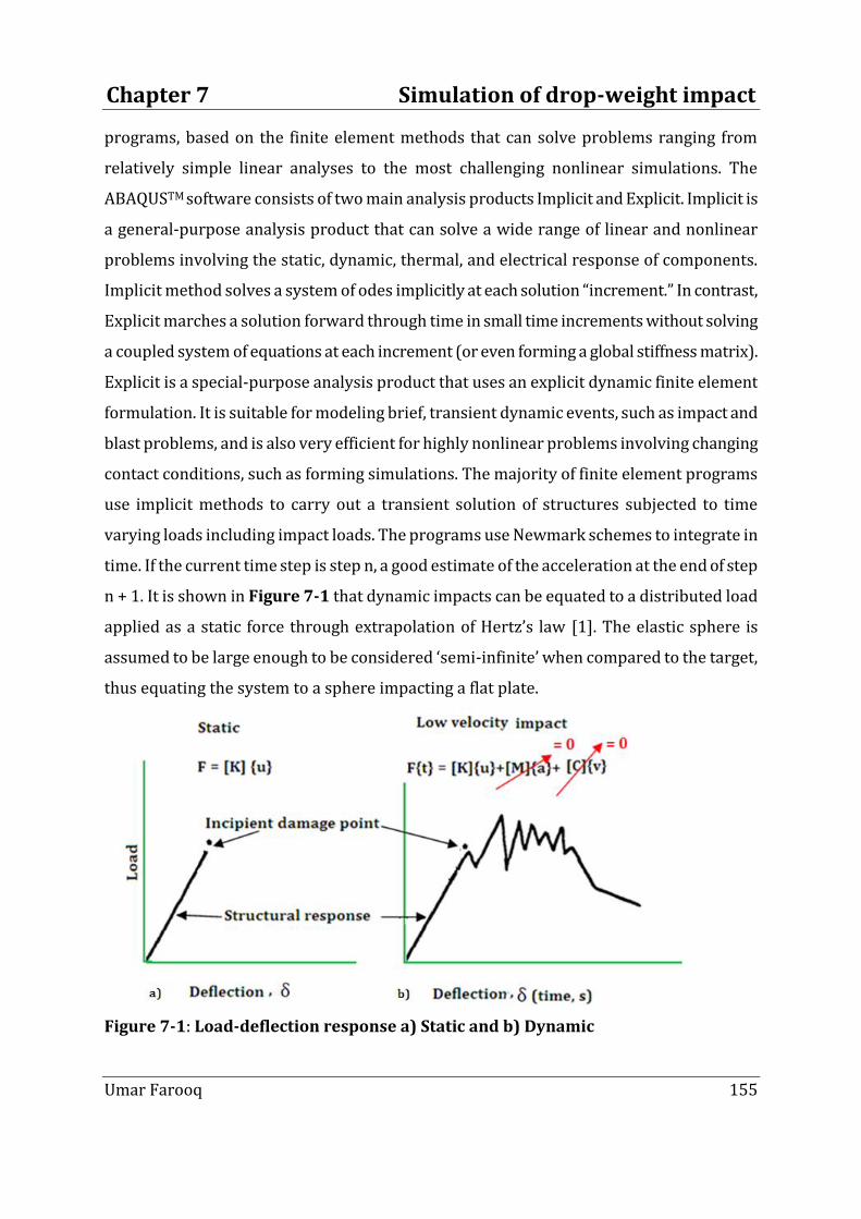
Chapter 7 Simulation of drop-weight impact
Umar Farooq 155
programs, based on the finite element methods that can solve problems ranging from
relatively simple linear analyses to the most challenging nonlinear simulations. The
ABAQUSTM software consists of two main analysis products Implicit and Explicit. Implicit is
a general-purpose analysis product that can solve a wide range of linear and nonlinear
problems involving the static, dynamic, thermal, and electrical response of components.
Implicit method solves a system of odes implicitly at each solution “increment.” In contrast,
Explicit marches a solution forward through time in small time increments without solving
a coupled system of equations at each increment (or even forming a global stiffness matrix).
Explicit is a special-purpose analysis product that uses an explicit dynamic finite element
formulation. It is suitable for modeling brief, transient dynamic events, such as impact and
blast problems, and is also very efficient for highly nonlinear problems involving changing
contact conditions, such as forming simulations. The majority of finite element programs
use implicit methods to carry out a transient solution of structures subjected to time
varying loads including impact loads. The programs use Newmark schemes to integrate in
time. If the current time step is step n, a good estimate of the acceleration at the end of step
n + 1. It is shown in Figure 7-1 that dynamic impacts can be equated to a distributed load
applied as a static force through extrapolation of Hertz’s law [1]. The elastic sphere is
assumed to be large enough to be considered ‘semi-infinite’ when compared to the target,
thus equating the system to a sphere impacting a flat plate.
Figure 7-1: Load-deflection response a) Static and b) Dynamic

Chapter 7 Simulation of drop-weight impact
Umar Farooq 156
In a low-velocity impact event the inertial terms and damping terms may be neglected as a
reasonable approximation of the system response. Static-governing Eq. (7-1) and dynamic
problems-governing Eq. (7-2) are solvable within these constraints.
𝑭 = [𝑲] 𝒖 (7-1)
𝑭 𝒕 = 𝑲 𝒖 + 𝑪 𝒖 + 𝑴 𝒖 (7-2)
Here F is the force, F(t) is time dependent force, [K], [M], and [C] are the
reduced/discretised stiffness, mass and damping matrices, respectively, the sizes for which
depend on the number of active degrees of freedom in the model. The relationships for
displacement, 𝒖 its first derivative velocity 𝒖 and second derivative acceleration 𝒖 are
shown. Problems involving enforced loads, for example, are solved for displacement at each
nodal point and stresses are calculated from these solutions. Results can be viewed
graphically on model contour plots and wireframe animation and through a hierarchy of
tabular output.
7.3 Simplified modelling of impact problem using contact law
Impact problem can be formulated as a beam struck transversally by a spherical mass m
with initial moving velocity v0 as shown in Figure 7-2. The impact to model the impact
dynamics on flexible beam is formulated to solve numerically the problem of central impact
of a sphere on a simply supported beam [13]. To obtain maximum deflection the quasi-
static analysis assumptions include:
a) impactor and target are isotropic
b) stiffness parameter Ki can be neglected for rigid impactor
c) radius of spherical impactor is R and radius of flat plate is infinite (∞).

Chapter 7 Simulation of drop-weight impact
Umar Farooq 157
Figure 7-2: Impactand local-global deformation
The contact deformation α defined as the difference between the displacement of the
impactor and that of the composite laminates, is given by the following:
𝜶 𝒕 = 𝒘𝒊 𝒕 − 𝒘𝒔 𝒕 (7-3)
Where: 𝛿𝑝 is plate deflection, 𝑤𝑖 𝑡 𝑎𝑛𝑑 𝑤𝑠 𝑡 are the displacement of impactor and
displacement of the impact point on the mid surface of the plate. The Hertz law is assumed
to be valid for the relation [14]:
𝜶 = 𝑲 𝑭 𝒕 𝟐
𝟑 (7-4)
The coefficient Fm is maximum impact force and α is indentation depth (the relative
approach of the striking body) F(t) is the contact force, and K is the Hertzian contact
constant given by the following:
𝒌 =𝟒
𝟑𝑹
𝟏𝟐
𝟏−𝝂𝒊𝟐
𝑬𝒊+
𝟏
𝑬𝟐 −𝟏
(7-5)
Where R: (1
𝑅=
1
𝑅1+
1
𝑅2), E1and ν are the radius, the Young’s modulus and the Poisson’s ratio
of the impactor and E2 is the transversal Young’s modulus of the plate. Contact force
between the impactor and the plate can be calculated using a modified Hertz indentation
law [13] proposed

Chapter 7 Simulation of drop-weight impact
Umar Farooq 158
𝑭 = 𝑲𝜶
𝟑𝟐 𝑭𝒐𝒓𝐥𝒐𝒂𝒅𝒊𝒏𝒈
𝑭𝒎 𝜶−𝜶𝟎
𝜶𝒎−𝜶𝟎 𝒒
𝑭𝒐𝒓 𝒖𝒏 − 𝒍𝒐𝒂𝒅𝒊𝒏𝒈 (7-6)
Where: q is experimental constant, subscript m means maximum indentation depth,
corresponding to Fm, before the unloading phase. The constant α0 is the permanent
indentation depth.
𝜶𝟎 = 𝜷 𝜶𝒄𝒓 − 𝜶𝟎 𝒊𝒇 𝜶𝒎 ≥ 𝜶𝒄𝒓
𝟎 𝒊𝒇 𝜶𝒎 ≤ 𝜶𝒄𝒓 (7-7)
Where: β is the experimental constant.
The dynamic of a rigid ball is given by the use of the Newton’s second law:
𝒎𝒊𝜶 𝒊 = −𝑭𝒄 (7-8)
Where: mi is the mass of the ball (impactor) and Fc is the contact force. In order to solve Eq.
(6-8) Newmark algorithm could be applied [59] and [60]. The dynamics of the plate and the
impactor for each time step, the algorithm is giving by the following:
𝜶𝒊 𝒏+𝟏 = 𝜶𝒊 𝒏 + ∆𝒕 𝜶 𝒊 + ∆𝒕𝟐
𝟒 𝜶 𝒊 𝒏 −
∆𝒕𝟐
𝟒𝒎𝒊 𝑭𝒄 𝒏+𝟏 (7-9)
Hence, from Hertz contact [13] not only the loading and un-loading force can be predicted
but dynamic of the impact event. Numerical solutions of the time-dependent Eq. (6-9) are
required. The Runge-Kutta methods are widely used for numerically estimating solutions to
differential equation of the form 𝑦 = 𝑓 𝑥, 𝑦 in both explicit and implicit applications. The
methods are ascribed to Euler for an explicit solution:
𝒚𝟏 = 𝒚𝟎 + 𝒉𝒇 𝒙𝟎, 𝒚𝟎 (7-10)
The backward Euler method is the simplest implicit method:
𝒚𝟏 = 𝒚𝟎 + 𝒉𝒇 𝒙𝟏, 𝒚𝟏 (7-11)
The notation 𝑥0, 𝑦0 is the initial point from which the method launches itself to generate
a new point 𝑥1, 𝑦1 ; where 𝑥1 = 𝑥0 + ℎ and h is the step size. The Euler forward method
is an explicit method. The expression for 𝑦1 depends only on 𝑥0 and 𝑦0. Backward Euler is
an implicit method, since the right-hand side also contains 𝑦1; that is, 𝑦1 is implicitly

Chapter 7 Simulation of drop-weight impact
Umar Farooq 159
defined. However, implicit and explicit algorithms are widely used for obtaining numerical
solutions of impact problems in computer simulation of physical processes.
7.3.1 Implicit method
In an implicit scheme, the displacement is not a function of time. Hence the velocities and
accelerations which are time derivatives of displacement turn out to be zero and the mass
and damping factors can be neglected. Euler forward and backward methods illustrate
solution process of explicit and implicit methods
𝒅𝒚
𝒅𝒕= −𝒚𝟐, 𝒚∈ 𝟎, 𝒂 (7-12)
with the initial condition 𝑦 0 = 1. Considering a grid 𝑡𝑘 = 𝑎 𝑘
𝑛 𝑓𝑜𝑟 0 ≤ 𝑘 ≤ 𝑛, that is, the
time step is ∆𝑡 = 𝑎 𝑛 and denote 𝑦𝑘 = 𝑦 𝑡𝑘 for each k. The simplest explicit and implicit
methods are used to discretise Eq. (7-12) based on the forward and backward Euler
schemes. The Forward Euler method
𝒅𝒚
𝒅𝒕 𝒌
=𝒚𝒌+𝟏−𝒚𝒌
∆𝒕= −𝒚𝒌
𝟐
Yields
𝒚𝒌+𝟏 = 𝒚𝒌 − ∆𝒕𝒚𝒌𝟐
for each 𝑘 = 0, 1, … , 𝑛; is an explicit formula for 𝑦𝑘+1. The Backward Euler method
𝒚𝒌+𝟏−𝒚𝒌
∆𝒕= −𝒚𝒌+𝟏
𝟐 is the implicit equation
𝒚𝒌+𝟏 + ∆𝒕𝒚𝒌+𝟏𝟐 = 𝒚𝒌 (7-13)
for 𝑦𝑘+1 compare this with formula (7-13) is given explicitly rather than as an unknown in
an equation. That is a quadratic equation having one negative and one positive root. The
positive root is picked because in the original equation, the initial condition is positive, and
then y at the next time step is given by
𝒚𝒌+𝟏 = −𝟏+ 𝟏+𝟒∆𝒕𝒚𝒌
𝟐∆𝒕 (7-14)

Chapter 7 Simulation of drop-weight impact
Umar Farooq 160
In the vast majority of cases, the equation to be solved when using an implicit scheme is
much more complicated than a quadratic equation, no exact solution exists, and root
finding algorithms such as Newton methods are applied. The implicit method is based on
Newark’s method, Newton-Raphson method etc. In order to solve an FEM problem using
implicit method, inversion of stiffness matrix is required. Very Large deformation problems
such as crash analysis can result in millions of degrees of freedom effectively increasing the
size of stiffness matrix. Larger the stiffness matrix longer is the computational time
required for its inversion. Hence there is a need for an explicit method which would
prevent the inversion of stiffness matrix. The Implicit method is a general-purpose analysis
technique that can solve a wide range of linear and nonlinear problems involving the static,
dynamic, thermal, and electrical response of components. Implicit method solves a system
of equations implicitly at each solution “increment.” The majority of finite element
programs use implicit methods to carry out a transient solution of structures subjected to
time varying loads including impact loads. Normally, these programs use Newmark
schemes to integrate in time and formulation allows pre-assumed-static as well as a
dynamic approach[13]. In the pre-assumed-static case where acceleration and velocity
forces are neglected, the load-displacement leads to Eq. (7-1) and Eq. (7-2) for the implicit
dynamic case. If the current time step is step ‘n’ an estimate of the acceleration at the end of
step n + 1 will be 𝑢 𝑛+1 . The Eq. (7-2) may be written at the next step as:
[𝑴]{𝒖 𝒏+𝟏} + [𝑪]{𝒖 𝒏+𝟏} + [𝑲]{𝒖𝒏+𝟏} = {𝑭𝒏+𝟏} (7-15)
Where:
𝑢 𝑛+1= estimated acceleration at step n+1
𝑢 𝑛+1= estimated velocity at step n+1
𝑢𝑛+1= estimated displacement at step n+1
𝐹𝑛+1= vector of externally applied loads at step n+1, and
Implicit methods are solved in time by applying Newmark method. Considering motion of
the impactor, the displacement can be calculated from the standard kinematic using
velocity and acceleration:
𝒖 = 𝒖 𝒕 + 𝟏
𝟐𝒖 𝒕𝟐 (7-16)

Chapter 7 Simulation of drop-weight impact
Umar Farooq 161
Based on the assumption that the acceleration varies linearly between two instants of time,
the resulting expression for the velocity and displacement vectors may be written as:
𝒖 𝒏+𝟏 = 𝒖 𝒏 + 𝟏 − 𝜷 𝒖 𝒏 + 𝜷𝒖 𝒏+𝟏 ∆𝒕 (7-17)
𝒖𝒏+𝟏 = 𝒖𝒏 + 𝒖 𝒏 ∆𝒕 + 𝟏
𝟐− 𝜶 𝒖 𝒏 + 𝜶𝒖 𝒏+𝟏 ∆𝒕𝟐 (7-18)
Where the parameters 𝛼 and 𝛽 indicate how much the acceleration at the end of the
interval enters into the velocity and displacements. The end of the interval ∆𝑡 can be chosen
to obtain the desired accuracy and stability. When 𝛽 = 12 and= 1
6 , Eqs. (7-17) and (6-
18) correspond to the linear acceleration method which can also be obtained from Wilson-
𝜃 algorithms (scheme when 𝜃 = 1). When = 12 𝑎𝑛𝑑 𝛽 = 1
4 the Eqs. (7-12) and (7-17)
corresponds to the constant acceleration between marching steps 𝑡𝑛 𝑎𝑛𝑑 𝑡𝑛+1. If
displacement is obtained by integration using the mean value theorem then the
displacement may be written as:
𝒖𝒏+𝟏 = 𝒖𝒏 + 𝒖 ∆𝒕 + 𝟏
𝟐𝒖 𝜷∆𝒕𝟐 (7-19)
Where:
𝒖 𝜷 = 𝟏 − 𝟐𝜷 𝒖 𝒏 + 𝟐𝜷𝒖 𝒏+𝟏 𝟎 ≤ 𝜷 ≤ 𝟏 (7-20)
Newmark integration parameters become the mid-points (𝛼 = 𝛽 = 1/2). The Eq. (7-17) and
(6-18) reduce to:
𝒖 𝒏+𝟏 = 𝒖 𝒏 + 𝜶𝒖 𝒏+𝟏∆𝒕 (7-21)
𝒖𝒏+𝟏 = 𝒖𝒏 + 𝜷𝒖 𝒏+𝟏∆𝒕𝟐 (7-22)
The Eq. (7-21) can be utilised to express 𝑢 𝑛+1 in terms of 𝑢𝑛+1and the resulting expression
can be substituted in Eq. (7-19) to express 𝑢 𝑛+1in terms of 𝑢𝑛+1. By substituting these
expressions for 𝑢 𝑛+1and 𝑢 𝑛+1into Eq. (7-19) the following relation is obtained for finding
displacement:
𝒖𝒏+𝟏 = 𝟏
𝜶 ∆𝒕 𝟐 𝑴 +
𝜷
𝜶∆𝒕 𝑪 + 𝑲
−𝟏

Chapter 7 Simulation of drop-weight impact
Umar Farooq 162
𝑭𝒏+𝟏 + 𝑴 𝟏
𝜶 ∆𝒕 𝟐𝒖𝒏 +
𝟏
𝜶∆𝒕𝒖 𝒏 +
𝟏
𝟐𝜶− 𝟏 𝒖 𝒏 + 𝑪
𝜷
𝜶∆𝒕𝒖𝒏 +
𝜷
𝜶− 𝟏 𝒖 𝒏 +
𝜷
𝜶− 𝟐
∆𝒕
𝟐𝒖 𝒏
(7-23)
The mass, damping, and stiffness matrices are assembled and dynamic equilibrium is
solved at each point in time. The displacement could be found directly by inversion of the
rigidity matrix, which is a classical inversion problem. It uses Gauss elimination, with its
usual matrix conditioning problems where computer time is proportional to the square of
the matrix size. All the matrices have to be inverted to determine displacement from Eq. (6-
18). Implicit solutions are unconditionally stable; therefore, time step size may be chosen
according to the required accuracy. However, solution procedure is complicated with
increasing degree of nonlinearities that leads to the inversion of larger matrices, the
associated time steps, and larger computing resources.
7.3.2 Explicit method
Explicit methods calculate the state of a system at a later time from the state of the system
at the current time, while implicit methods find a solution by solving an equation involving
both the current state of the system and the later one. Mathematically, if 𝑌 𝑡 is the current
system state and 𝑌 𝑡 + ∆𝑡 is the state at the later time (∆𝑡 is a small time step), then, for an
explicit method
𝒀 𝒕 + ∆𝒕 = 𝑭 𝑭 𝒕 (7-24)
while for an implicit method one solves an equation:
𝑮 𝒀 𝒕 , 𝒀 𝒕 + ∆𝒕 = 𝟎 (7-25)
It is clear that to find 𝑌 𝑡 + ∆𝑡 implicit methods require an extra computation to solve Eq.
(7-25) that can be much harder to implement. Implicit methods are used because many
problems arising in practice are stiff, for which the use of an explicit method requires
impractically small time steps ∆𝑡 to keep the error in the result bounded (stability). For
such problems, to achieve given accuracy, it takes much less computational time to use an
implicit method with larger time steps, even taking into account that one needs to solve an
Chapter 7 Simulation of drop-weight impact
Umar Farooq 163
equation of the form Eq. (7-25) at each time step. That said whether one should use an
explicit or implicit method depends upon the problem to be solved. As opposed to implicit
methods, explicit scheme is a function of time. Being a function of time, the velocity and
acceleration as well as the mass and damping need to be considered in this scheme. In an
explicit method, central difference time integration is used to calculate field variables at
respective nodal points. Since only a numerical solution is possible for a nonlinear ordinary
differential equation, this method is particularly suited for nonlinear problems. It requires
the inversion of the lumped mass matrix as opposed to that of the global stiffness matrix in
the implicit methods. The equation of motion is evaluated at the previous time step tn-1,
where tn is the current time step. The explicit method or algorithm works in time step
increments i.e. the displacements are calculated as the time proceeds. The term “explicit”
refers to the fact that the state at the end of the increment is based solely on the
displacements, velocities, and accelerations at the beginning of the increment. For impact
problems with an impact velocity greater than 1m/s, it is essential that explicit method is
applied. The Explicit method available in special-purpose analysis software routines
suitable for modelling brief, transient dynamic events, such as impact and blast problems,
and highly nonlinear problems involving changing contact conditions such as process
forming. The explicit algorithm can model discontinuous nonlinearities such as contact and
failure more easily where the stiffness changes due to structural deformation. Fully
populated matrix inversions are not required for explicit methods. The motion is used to
obtain acceleration. At the beginning of the increment the program solves for dynamic
equilibrium, which states that the nodal mass matrix times the nodal accelerations, equals
the net nodal forces (the difference between the external applied forces, and internal
element forces):
𝑴 𝒖 = 𝑭𝒆𝒙𝒕𝒆𝒓𝒏𝒂𝒍 + 𝑭𝒊𝒏𝒕𝒆𝒓𝒏𝒂𝒍 (7-26)
Assuming acceleration is constant through the time step, velocities and accelerations are
found by central difference method:
𝒖 𝒏 =𝟏
𝟐∆𝒕 𝒖𝒏+𝟏 − 𝒖𝒏−𝟏 (7-27)

Chapter 7 Simulation of drop-weight impact
Umar Farooq 164
𝒖 𝒏 =𝟏
∆𝒕 𝟐 𝒖𝒏+𝟏 − 𝟐𝒖𝒏 + 𝒖𝒏−𝟏 (7-28)
The accelerations are integrated through time using the central difference rule, which
calculates the change in velocity assuming that the acceleration is constant.
Thus the Eq. (7-19) can be written as:
𝑴 𝟏
∆𝒕 𝟐 𝒖𝒏+𝟏 − 𝟐𝒖𝒏 + 𝒖𝒏+𝟏 + 𝑪
𝟏
𝟐∆𝒕 𝒖𝒏+𝟏 − 𝒖𝒏+𝟏 + 𝑲 𝒖𝒏 = 𝑭𝒏
(7-29)
The Eq. (6-29) can be re-arranged to obtain
𝑴 𝟏
∆𝒕 𝟐+ 𝑪
𝟏
𝟐∆𝒕 𝒖𝒏+𝟏 = 𝑭𝒏 − 𝑲 −
𝟐
∆𝒕 𝟐 𝑴 𝒖𝒏 − 𝑴
𝟏
∆𝒕 𝟐− 𝑪
𝟏
𝟐∆𝒕 𝒖𝒏−𝟏
(7-30)
Thus Eq. (7-30) gives solution vector 𝑢𝑛+1 once 𝑢𝑛 and 𝑢𝑛−1 are known. The method
integrates accelerations exactly. The lump mass matrix ‘M’ is a diagonal which assumes
inconsistent structures. Inversion of the matrix is direct and trivial. Therefore, Eq. (7-30) is
a set of independents. Typically, explicit time steps are orders of magnitude less than those
used with implicit codes. The only difficulty is to ensure stable time integration for very
small time increments (stability is the duration that the stress wave crosses the smallest
element). Explicit methods can be made unconditionally stable if the time step is chosen to
be less than the time taken for a stress wave to cross the smallest element in the mesh.
Figure 7-3 shows propagation of stress waves where artificial mass scaling (increasing
density) method for a material medium a stable time increment is achieved.

Chapter 7 Simulation of drop-weight impact
Umar Farooq 165
Figure 7-3: Time step and stress wave relationship
Where:
L = minimum element length (characteristic element dimension)
𝑐 = 𝐸
𝜌
1
1−𝜈2 is the dilatational speed of sound wave for 2D element
𝜈 = Poisson’s ratio
𝜌 = density
∆𝑡 = 1
𝐶 𝐿 the smallest transit time of dilatational waves to cross any element in the mesh
The critical time is:
∆𝑡𝑐𝑟𝑖𝑡𝑖𝑐𝑎𝑙 = 2
𝜔𝑚𝑎𝑥 1 + 𝜉2 − 𝜉
Where:
𝜔𝑚𝑎𝑥 = the highest frequency in the system
𝜉 = damping ratio, the fraction of critical damping in the highest mode.
This may result in reducing considerable computing time by using explicit routine with a
quasi-static approach for solving the small strain rate problems. The explicit procedure
always uses a diagonal matrix hence accelerations computations are trivial without large
matrix (only a diagonal matrix). The acceleration of any node is determined completely by
its mass and the net force acting on it, making the nodal calculations computationally
Chapter 7 Simulation of drop-weight impact
Umar Farooq 166
inexpensive. The algorithm produces robust solution procedures even for high degree of
nonlinearities.
Once displacements are found strains and stresses can be determined. For a symmetric
laminate loaded in one plane of bending only (as a case for the simply supported plate) the
curvatures are given as:
𝒌𝒙𝒙
𝒌𝒚𝒚
𝒌𝒙𝒚
= 𝑫𝟏𝟏 𝑫𝟏𝟐 𝑫𝟏𝟔
𝑫𝟐𝟏 𝑫𝟐𝟐 𝑫𝟐𝟔
𝑫𝟏𝟔 𝑫𝟐𝟔 𝑫𝟔𝟔
−𝟏
𝑴𝒙𝒙
𝑴𝒚𝒚
𝑴𝒙𝒚
(7-31)
From Eq. (7-30) it is apparent that the twisting curvature is nonzero in Eq. (7-31). Applying
Hooke’s law to the orthotropic laminate the stress in kth layer is then:
𝝇𝒙𝒙𝒌 = 𝒛𝑴𝒙𝒙 𝑸 𝟏𝟏𝑫𝟏𝟏
−𝟏 + 𝑸 𝟏𝟐𝑫𝟏𝟐−𝟏 + 𝑸 𝟏𝟔𝑫𝟏𝟔
−𝟏 (7-32)
The expression in Eq. (7-32) calculates which layer breaks in first in tension. The same
process can be applied to predict failure stresses corresponding to the applied loading for
multi-layered composites.
The implicit methods are the most efficient way to handle so-called stiff differential
equations, which are differential equations that usually feature a rapidly decaying solution.
Explicit methods need to take very tiny values of h to accurately estimate the solution, and
this takes lots of time. Implicit methods allow for a more reasonably sized h but required to
use an associated method for solving the implicit equation, like Newton-Raphson.
Moreover, implicit and explicit are two types of approached that can be used to solve the
finite element problem. The implicit approach is useful in problems in which time
dependency of the solution is not an important factor (e.g. static structural, harmonic,
modal analysis etc.) whereas explicit dynamics approach is most helpful in solving high
deformation time dependent problems. Based on computational performance efficiency
comparison explicit method was selected for the drop-weight simulation part of the work.

Chapter 7 Simulation of drop-weight impact
Umar Farooq 167
7.4 Materials and geometric properties of laminates and impactors
The symmetrical laminates of layups code [0/45/-45/90]ns where the subscript n varies
from 1, 2, and 3 for sequence repetitions and s stands for symmetry. The schematic of test
laminate is shown in Figure 7-4 (a). In Figure 7-4 (b) each fill fibre ply goes over four plies
before going under fifth one. This configuration is called a 5-harness satin weave.
Figure 7-4: 8-Ply symmetric laminates
The test specimens consist of 150 mm x 120 mm plane areas (proposed in [1]) with
variable thicknesses from 2.3, 4.6, and 7.2 mm as shown in Figure 7-5. The total average
thickness of every plies in a specific lay-up is assumed of uniform material properties.

Chapter 7 Simulation of drop-weight impact
Umar Farooq 168
Schematic of four ply quasi-isotropic specimen.
Figure 7-5: a) 8-ply, b) 16-ply, and c) 24-ply specimens
The tests laminates are made of aerospace grade carbon fibre reinforced toughened epoxy
infused. Test laminates were provided by the industry, fabricated using two types of fibre
reinforcements: IM7/8552 named Material A [1] and Fibre dux T300 914C-833-40
embedding fibre horns technique named Material B Table 7-1.
Table 7-1: Material B properties [4]
Property Units Fibredux T300
Tensile Modulus (E11) GPa 230
Tensile Modulus (E22 = E33) GPa 21
In-plane Shear Modulus (G12= G13) GPa 88
Out-of-plane Shear Modulus (G23) GPa 11
Poisson’s Ratio (12) - 0.2
Longitudinal Tensile Strength (𝑋𝑇) MPa 650
In-plane Shear Strength (𝑆12) MPa 180
Longitudinal Compressive Strength (𝑌𝑇) MPa 650
Transverse shear strength (𝑆13 = 𝑆23) MPa 32
Inter-laminar shear strength (𝑍𝑇) MPa 10

Chapter 7 Simulation of drop-weight impact
Umar Farooq 169
The impact affected area consists of a 50 mm diameter at central region for all specimens.
All the areas were in circular shape as shown in Figure 7-6 (b). The specimens are
required to be impacted with impactors at the centre. Round and flat nose shape impactor
made of steel and consisting of three parts: the crosshead, shank, and nose were used as
shown in Figure 7-6(c) & (d) that can be changed. The flat type impact is regarded
common danger in aerospace industry hence the nose shape was emphasized in this study.
The impactors used were made of stainless steel. Both impactors have shank of diameter 20
mm reducing to 10 ± (0.18) mm with the round impactor having a nose shape radius of 5 ±
(0.15) mm and flat impactor ground flat impact face.
Figure 7-6: a) Schematic of a) specimen, b) cut-out of impact affected zone; c) round
nose , and d) flat nose shape impactors
Investigations of the impact response of the specimens were desired to determine
deflections, velocities, accelerations, stresses, and strains to predict damage and failure
modes and their locations.
4.8 & 7.2
c) d)
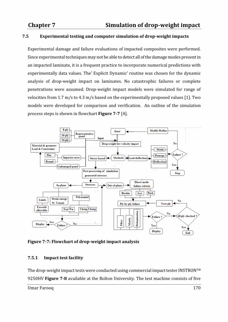
Chapter 7 Simulation of drop-weight impact
Umar Farooq 170
7.5 Experimental testing and computer simulation of drop-weight impacts
Experimental damage and failure evaluations of impacted composites were performed.
Since experimental techniques may not be able to detect all of the damage modes present in
an impacted laminate, it is a frequent practice to incorporate numerical predictions with
experimentally data values. The’ Explicit Dynamic’ routine was chosen for the dynamic
analysis of drop-weight impact on laminates. No catastrophic failures or complete
penetrations were assumed. Drop-weight impact models were simulated for range of
velocities from 1.7 m/s to 4.3 m/s based on the experimentally proposed values [1]. Two
models were developed for comparison and verification. An outline of the simulation
process steps is shown in flowchart Figure 7-7 [4].
Figure 7-7: Flowchart of drop-weight impact analysis
7.5.1 Impact test facility
The drop-weight impact tests were conducted using commercial impact tester INSTRONTM
9250HV Figure 7-8 available at the Bolton University. The test machine consists of five

Chapter 7 Simulation of drop-weight impact
Umar Farooq 171
main components two rectangular steel bar and two steel rods. Besides, two components
assemble with bearings on the rods. Elevator system has a motor, cables and an electrical
magnet. Control unit manages elevator system, hydraulic system for grips and
electromagnet. The main block, control console, and a computer connected to data
acquisition system consists of piezoelectric load sensor, accelerometer, drop-weight,
release and crosshead brake as catching mechanism attached to the test rig prevents
multiple impacts on the laminate by the impactor. If the impactor rebounds after the
impact, the brake system turns on and catches impactor immediately.The tup is placed on
the impactor used to strike the laminate. Within the tup is a strain gauge that measures the
change in strain against time as the impactor strikes the laminate. The signal conditioning
unit removes the noise associated with the signal and the data display system plots the
measured data. The available drop-weight tower was used to test the impact resistance of
composite laminates it consists of a base plate with the fixture mechanism and a frame
supporting the guide for a drop weight. The base plate and frame are made of massive steel
parts to restrain the vibrations travelling through the tower.
Its principal features are:
1) A control panel is provided to manually enter necessary input and push button to
release the drop weight assembly from a preselected drop position. The position,
based on the required impact energy, can be adjusted by moving the clamp frame up
and down and clamping it to the guide columns using the clamp knobs.
2) The drop weight assembly is the core of the Dynatup impact instrument. This
assembly consists of three parts are as follows. The drop weight consists of the mass
for the impact testing. The drop weight assembly is a framework of weights and
plates bolted together and weights can be stacked securing hand-knob
3) Anvils are fixtures that hold specimens during testing. Different styles of anvil are
available to accommodate various test specifications and techniques
4) The impact force applied on the specimen is measured by the tup of the drop
weight assembly. It consists of two parts, the tup: which is a load cell for measuring
force, and the tup to insert impact head which is the impactor that actually strikes
the specimen.

Chapter 7 Simulation of drop-weight impact
Umar Farooq 172
5) The impactor was dropped precisely onto the specimen with the help of a guiding
mechanism. This guiding mechanism consists of two vertical bars (columns), base
plate, back and top support and table. The drop weight assembly drops free fall on
the guide columns via holes in its upper and lower guide blocks. The two guide
columns bolted to the base plate and the top support. The back support provides
rigidity and vertical stability to the drop tower.
6) A crosshead brake attached to the test rig prevents multiple impacts on the
specimen by the impactor.
7) The impact tower is instrumented with all necessary sensors to monitor the impact
force, the dynamic response of the plate and the incident and rebound velocities.
The tip of the impactor is equipped with a piezoelectric force transducer in order to
monitor the contact force. A laser Doppler vibrometer head capable of measuring
single point velocity response is mounted on the frame of the tower. The base of the
tower is also equipped with an accelerometer. Two light barriers are mounted on
the guiding rail in order to trigger the acquisition devices and measure the incident
and rebound velocity of the drop weight.
8) The ImpulseTM data acquisition, analysis software, velocity detector, and data
visualization using dedicated DSP technology to deliver high performance capability
to meet a wide range of impact testing applications. In addition, the software can
generate a variety of reports.
9) Specifications
Maximum velocity 20 m/s; Energy range: 2.6-1603 J
Maximum Drop Height: 1.25 m; Drive speed: 1600 mm/min
Maximum load for 3 sensors: 450N, 2.2 kN, 4.5 kN, and 22.2 KN
Drop-weight ranges:
Light: 2.7-14.7 kg, Medium: 4.7-23.7 kg, and Maximum: 24.2-80.5 kg
The arrows point towards load-cell where impactor will be fitted and towards the fixture
where undamaged laminate will be clamped. Impactor will be released to make an impact
on the laminate. Then impacted laminates will be taken out of the fixture to evaluate the

Chapter 7 Simulation of drop-weight impact
Umar Farooq 173
damage as indicted by arrows in exploded view. Initially, two impact tests were performed
on typical 8-Ply laminates by both the flat and round nose impactors at 1.7 m/s velocity.
Figure 7-8: INSTRONTM 9250HV impact test machine
7.5.2 Impact test procedure
The laminates were impacted in accordance with the accepted American standard testing
method for measuring damage resistance of a fibre-reinforced polymer matrix composite to
a drop weight impact event (ASTM: D7136). Prior to impacting, the specimen was tightly
clamped around end boundary. The target holder sandwiches specimen between two
rectangular steel plates that had circular central holes (for 50 mm diameters test area). All
tests were performed at room temperature. Experiments were conducted in a manner such
that complete failure of the specimen did not occur. During each test, initial height was
adjusted from the drop-weight height release levels to hit the specimen with a selected

Chapter 7 Simulation of drop-weight impact
Umar Farooq 174
velocity. The impact velocity (energy) was also possible to control by adding metal slabs
(weights) since design of the machine does not permit to change mass of the impactor.
Similarly, adjustments were made to ensure that the impact occurs at the centre of the
laminate under the impactor head. To calibrate the brake system, the impactor was
lowered to touch the surface of the specimen. Once the machine is set to its correct
configuration and all data acquisition software is running, the mass is released and allowed
to impact the specimen. Few actions were necessary before conducting the test to prior
calibrate the testing:
(1) The tower's specifications, as well as the sample's specifications, were checked
against the ASTM standards prior to testing. The laminate types, impactor, and
support ring diameters were the same as used in static tests.
(2) Adjusting the drop weight height, setting selection of drop weight mass, and velocity
detector. The drop weight mass and the drop weight height determine the impact
energy just before the impact.
(3) Force sensor mounted between impactor and drop weight. Total mass of impactor
used, brake system, the impactor was touched surface of sample and so, two optical
sensors was calibrated.
(4) There is no mechanism available for conducting a test to simultaneously triggering
of the following sequence was carried out before dropping the mass on to the
specimen:
(a) First the ‘Impulse Data Software’ was switched ON and
(b) necessary data were input such as mass of drop weight assembly, height,
customising data logging files, then the ‘BUTTON’ was switched ON. The impact test
was then carried out by releasing the drop weight from the release button. The data
from the files were retrieved and read after the impact and switched was turned
OFF.
(5) Capturing the data and analysis, two separate sets of data were captured:
(a) one from the ‘INSTRONTM tester data acquisition system’ and
(b) the other from the ‘Low impedance voltage mode system’.

Chapter 7 Simulation of drop-weight impact
Umar Farooq 175
After the impact, raw data has been exported to Microsoft Excel and analysed. Once the
machine is set to its correct configuration and all data acquisition software is running
further tests were conducted. In drop weight impact testing, a mass is raised to a known
height and released and allowed to impact the plate. The composite panels and impactors
used in this work were based on the samples depicted in Figure 7-6 and tests were
selected from the flowchart Figure 7-7. The mass of the impactor and the drop height are
the variables, allowing for a wide range of impact energies. To perform impact, the
impactor is lifted with electromagnet to appropriate drop height. At the same time,
ImpulseTM, which is data logger program, was started in the computer. Then, electromagnet
is closed and impactor dropped onto the sample. As the impactor dropped and approached
the coupon, its time trigger passed through a time sensor right before contact-impact
occurred. The initial velocity was then calculated from the distance between the two edges
on the time trigger and the time interval they passes through the sensor. Once impact
begins, the contact forces at many consecutive instances were detected by the force
transducer attached to the impactor. The force history was recorded by the data acquisition
system. Data points collected during a test are up to 16000 for each channel. Sampling rate
is 1kH-2MHz for each channel. Acceleration of the impactor is obtained dividing difference
between impact force and total weight of the impactor to total weight of the impactor
deflection derives from a double integration of acceleration of the impactor. Data took from
the force sensor is sent to the computer. A program written in the software calculated and
plotted force-time curve. Other curves were calculated by these data. Specimens were
impacted at constant weight for all the desired cases with different impact
velocities/energies. Due to the non-linear behaviour of composite materials resulting from
many concurrent damage mechanisms that may occur from impact loading such as fibre
breakage, matrix cracking, delamination, back-face splitting or any combination of these,
four or five specimens were impacted under each test condition. All the results were
collected by data acquisition system. Then the force/displacement curve were plotted
which gives an idea of impact plates behaviour. The impact energy is the area occupied by
this curve. The data obtained from the test can be examined to see the impact resistance of
the plate. The data is plotted as force, energy, or displacement vs time. Time gives
information about how the material behaves during the impact process. The data is not
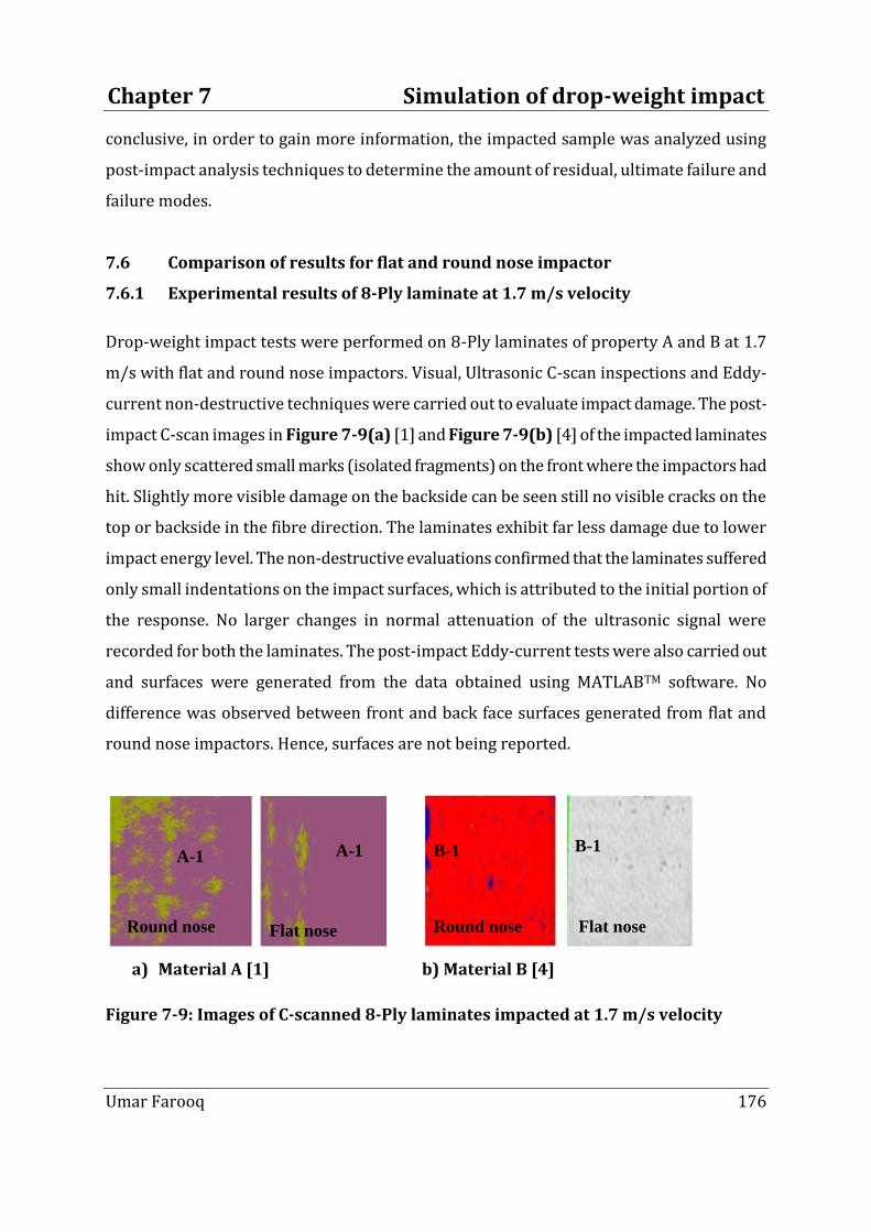
Chapter 7 Simulation of drop-weight impact
Umar Farooq 176
conclusive, in order to gain more information, the impacted sample was analyzed using
post-impact analysis techniques to determine the amount of residual, ultimate failure and
failure modes.
7.6 Comparison of results for flat and round nose impactor
7.6.1 Experimental results of 8-Ply laminate at 1.7 m/s velocity
Drop-weight impact tests were performed on 8-Ply laminates of property A and B at 1.7
m/s with flat and round nose impactors. Visual, Ultrasonic C-scan inspections and Eddy-
current non-destructive techniques were carried out to evaluate impact damage. The post-
impact C-scan images in Figure 7-9(a) [1] and Figure 7-9(b) [4] of the impacted laminates
show only scattered small marks (isolated fragments) on the front where the impactors had
hit. Slightly more visible damage on the backside can be seen still no visible cracks on the
top or backside in the fibre direction. The laminates exhibit far less damage due to lower
impact energy level. The non-destructive evaluations confirmed that the laminates suffered
only small indentations on the impact surfaces, which is attributed to the initial portion of
the response. No larger changes in normal attenuation of the ultrasonic signal were
recorded for both the laminates. The post-impact Eddy-current tests were also carried out
and surfaces were generated from the data obtained using MATLABTM software. No
difference was observed between front and back face surfaces generated from flat and
round nose impactors. Hence, surfaces are not being reported.
a) Material A [1] b) Material B [4]
Figure 7-9: Images of C-scanned 8-Ply laminates impacted at 1.7 m/s velocity
B-1 B-1 A-1 A-1
Flat nose Round nose Flat nose Round nose
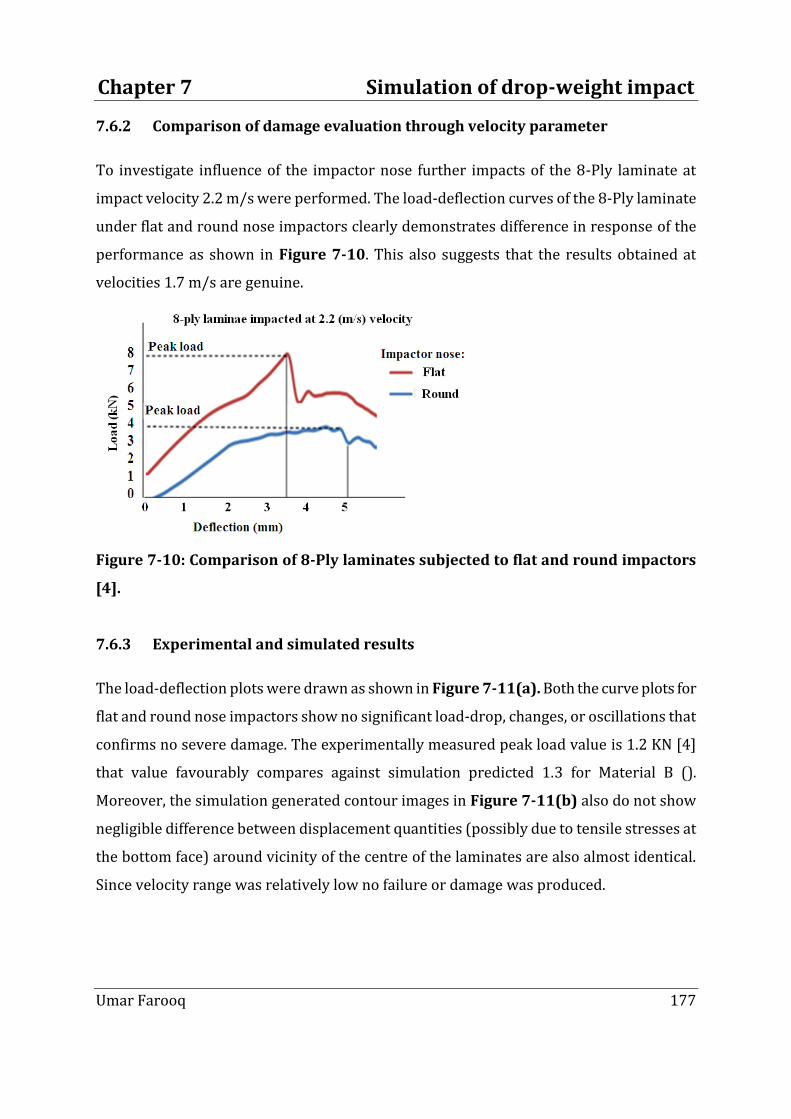
Chapter 7 Simulation of drop-weight impact
Umar Farooq 177
7.6.2 Comparison of damage evaluation through velocity parameter
To investigate influence of the impactor nose further impacts of the 8-Ply laminate at
impact velocity 2.2 m/s were performed. The load-deflection curves of the 8-Ply laminate
under flat and round nose impactors clearly demonstrates difference in response of the
performance as shown in Figure 7-10. This also suggests that the results obtained at
velocities 1.7 m/s are genuine.
Figure 7-10: Comparison of 8-Ply laminates subjected to flat and round impactors
[4].
7.6.3 Experimental and simulated results
The load-deflection plots were drawn as shown in Figure 7-11(a). Both the curve plots for
flat and round nose impactors show no significant load-drop, changes, or oscillations that
confirms no severe damage. The experimentally measured peak load value is 1.2 KN [4]
that value favourably compares against simulation predicted 1.3 for Material B ().
Moreover, the simulation generated contour images in Figure 7-11(b) also do not show
negligible difference between displacement quantities (possibly due to tensile stresses at
the bottom face) around vicinity of the centre of the laminates are also almost identical.
Since velocity range was relatively low no failure or damage was produced.

Chapter 7 Simulation of drop-weight impact
Umar Farooq 178
Figure 7-11: Comparison of 8-Ply laminates subjected to flat and round impactors.
Comparisons of the non-destructive evaluations, experimental plots, and simulation
contours show negligible difference by impactor’s nose up to a velocity of 1.7 m/s at initial
impact. This confirms that internal ply-by-ply damage for different nose shape impactors
cannot be readily evaluated through load-deflection method at relatively lower velocity.
Hence, further studies are carried out at relatively higher velocity range.
7.6.4 Comparison of the results through delaminated zone ratios
Tests were carried out according to the plan shown in Table 7-2 for 8-, 16-, and 24-Ply
laminates.
Table 7-2: Test plan of the selected simulation cases
Laminate
lay-up
Average
thickness
(±0.02) mm
Test code
Velocity
(±0.2)m/s
Flat Round
8-Ply 2.4 A-1 B-1 1.7
8-Ply 2.4 A-2 B-2 2.2
16-Ply 4.8 A-3 B-3 3.12
24-Ply 7.2 A-4 B-4 3.12
24-Ply 7.2 A-5 B-5 4

Chapter 7 Simulation of drop-weight impact
Umar Farooq 179
Visible damage that occurs from an impact event can be easily approximated. However,
damage is not always apparent, although there can be severe underlying damage. The
ultrasonic C-Scan and Eddy-current non-destructive damage evaluation techniques are
widely used in aerospace industry to produce a planar indication of the type and extent of
damage. To approximate delaminated area, meshing grids on all the impacted laminates
were projected on the scanned images and surfaces. The delaminated area is assumed to
map on circles by adding or subtracting rectangular mesh elements or cells as shown in
Figure 7-12.
Figure 7-12: Mesh grid projected on 8-Ply C-Scanned laminate [4]
A plane (X, Y) coordinate system was also assumed to locate initial and final positions of the
diameter of the delaminated area. The delaminated area is then divided by the laminate
area to obtain a ratio of the approximate delaminated area. A typical example of 8-Ply
laminate is computed in the MATLABTM code in Table 7-3. The same code was executed to
approximate delamination ratios of the other scanned laminates.
Length: 4mm
Width:
2mm

Chapter 7 Simulation of drop-weight impact
Umar Farooq 180
Table 7-3: Algorithm approximating the delaminated area [4]
%******************************************************************* ||
% MATLAB PROGRAM TO PREDICT RATIO OF DELAMINATED AREA ||
%******************************************************************* ||
% Example 1: dimensions of Laminate (800 mm x 710 mm)
length= input('Please enter length > 1');disp(length)
height= input('Please enter height > 1') ; disp (height)
area1 = length * height; fprintf ('Laminate area is =', area1)
% Dimensions of delaminated zone
% Coordinates of delaminated area (x = 460 & 310, y=300 & 400)
point1= input('Please enter x-coordinate 1');disp(point1)
point2= input('Please enter x-coordinate 2');disp(point2)
xx=(point2-point1)^2
point1= input('Please enter y-coordinate 1');disp(point1)
point2= input('Please enter y-coordinate 2');disp(point2)
yy=(point2-point1)^2; diameter =sqrt(xx+yy)
area2=pi*(diameter/2)^2; fprintf ('Delaminated area is =%f', area2)
area3=(area2/area1)*100
fprintf('Delamination ratio is = %f',area3)
Comparison of the selected results from flat and round nose impactors on 8-, 16-, and 24-
Ply laminates for the approximate ratios of the delaminated areas is shown in Table 7-3.
The tabular quantities for the other laminates in the Table 7-4 show consistent behaviour.

Chapter 7 Simulation of drop-weight impact
Umar Farooq 181
Table 7-4: Comparison of delaminated ratios [4]
Velocity
m/s
Ratios of delaminated area
8-Ply 16-Ply 24-Ply
Flat
nose
Round nose Flat nose Round nose Flat nose Round nose
1.7 0.8 0.5 0.2 0.15 0.12 0.1
3.12 8.3 7.9 11.4 14.17 13.7 12.17
4 18.6 18.12 20.88 19.4 23.8 18.2
Delaminated ratio increases with increased impact velocities. Discrepancies under 8-Ply
laminates’ delaminated ratios are due to perforation of the laminates. Under increased
velocities the relatively thin laminates perforate and this leads to discrepancies in the
approximation the damaged area. Comparisons of selected results, scanned images, and
Eddy-current surfaces were also carried out for 8-Ply, 16-Ply, and 24-Ply laminates
impacted from round nose impactors at velocity 3.12 m/s. Moreover, delaminated area
(surface area) increases as laminate thickness increases. Delaminated ratios of the top and
bottom surfaces were averaged to compare against the scanned images. Comparisons in a
sets of C-Scanned images with damage zone diameters: 3 to 8 mm and Eddy-current
surfaces with damage zone diameters: 4 to13 mm are shown in Figure 7-13. The
comparison of the scanned images and surface plots show consistent behavior. Moreover,
delaminated zone (surface area) increases as laminate thickness increases. Peaks of the
surfaces indicate internal depth of the damage.
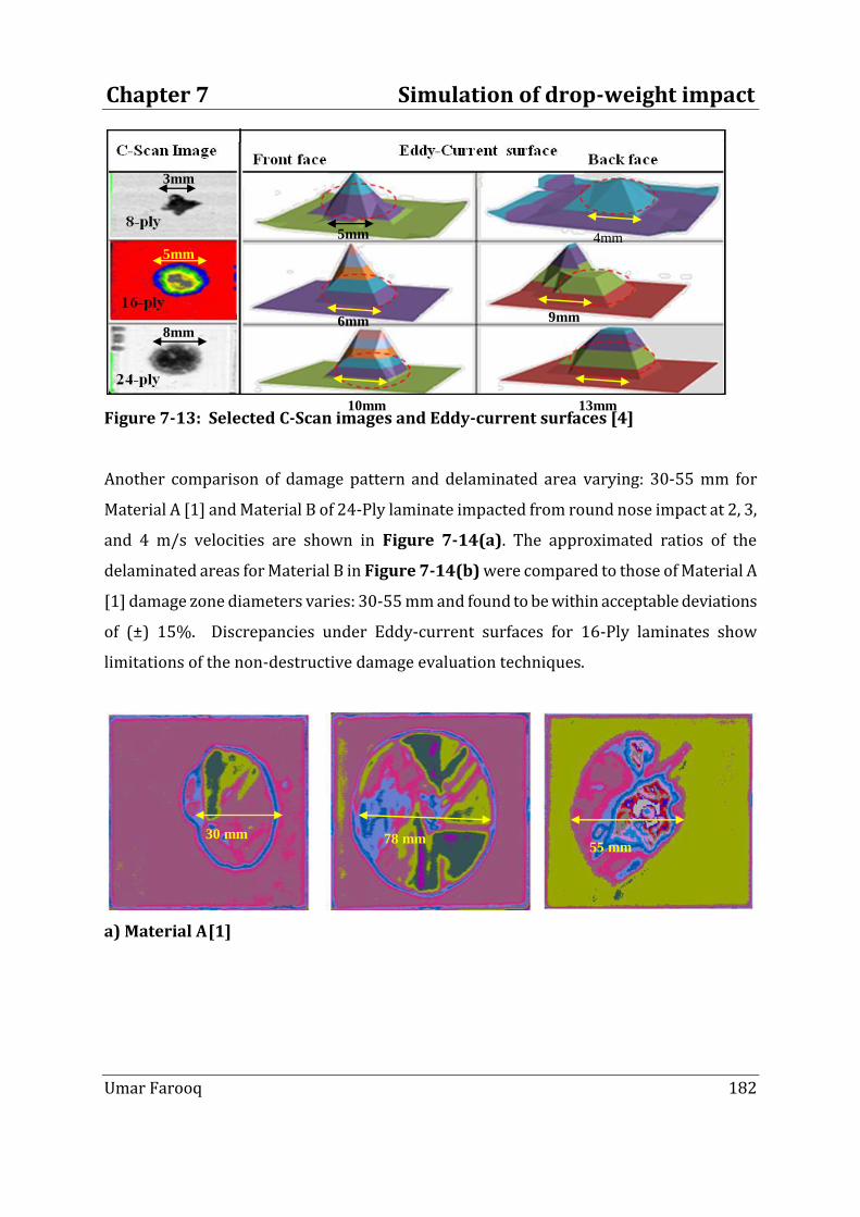
Chapter 7 Simulation of drop-weight impact
Umar Farooq 182
Figure 7-13: Selected C-Scan images and Eddy-current surfaces [4]
Another comparison of damage pattern and delaminated area varying: 30-55 mm for
Material A [1] and Material B of 24-Ply laminate impacted from round nose impact at 2, 3,
and 4 m/s velocities are shown in Figure 7-14(a). The approximated ratios of the
delaminated areas for Material B in Figure 7-14(b) were compared to those of Material A
[1] damage zone diameters varies: 30-55 mm and found to be within acceptable deviations
of (±) 15%. Discrepancies under Eddy-current surfaces for 16-Ply laminates show
limitations of the non-destructive damage evaluation techniques.
a) Material A [1]
30 mm 78 mm 55 mm
3mm
5mm
8mm
5mm
6mm
10mm 13mm
9mm
4mm

Chapter 7 Simulation of drop-weight impact
Umar Farooq 183
b) Material B
Figure 7-14: Comparison of 24-Ply laminate damage pattern [4]
7.7 Theoretical aspects of stress-based methodology
Materials’ strength can be expressed in terms of stresses or strains beyond certain values a
structure fractures or fails. After failure is detected the structural component can no longer
support the loads acting on it and fulfill the function for which it was designed. A failure
criterion is needed to hypothesize the loading response and failure limits of stress or strain
of a structure. The criteria to predict failure can also be utilised to predict location of weak
and strong locations and directions. The information could be very useful in designing
structural components and calculating margin of safety. The failure criteria are widely used
to define failure of unidirectional composite materials and are already implemented in
different finite element codes. A complete review and description of the different failure
criteria for composite materials are listed. A shortcoming of Tsai-Hill and Tsai-Wu criteria
is that they do not explicitly differentiate matrix failure from fibre failure. Quadratic criteria
fit well to experimental data under biaxial loading as long as the two interacting stresses
affect the same failure mechanism. This is the case of the interaction between in-plane
normal and shear stresses, because both stresses produce matrix failure. When two
interacting failure mechanisms are different, such as longitudinal failure and transverse
failure, the quadratic criteria forces as artificially smooth transition from one failure into
the other. The interactive failure criteria predict a given set of stresses that produce failure
but they do not predict the mode of failure. Hashin [111] set of interactive failure criteria in
which distinct failure modes are modelled, the following 3D failure criteria for
unidirectional composites that use more than a single stress component to evaluate
24 mm 73 mm 75 mm
Chapter 7 Simulation of drop-weight impact
Umar Farooq 184
different failure modes. He defined a general failure criterion in terms of the stress
invariants for a transversely isotropic material. Failure indices of the criteria are related to
fibre and matrix failures and involve four failure modes. Additional failure indices result
from extending the criteria to three-dimensional problems for the transverse stress
components.
In order to predict impact response of composite laminates through stress-based analysis,
the first step is to determine the impact induced local stresses in the structure to compare
them to a set of allowable values. The off-axis (±θ) ply orientations and different Poisson
ratios generate shear coupling when plies undergo shear deformations thus their effects
generate through-thickness stresses. The through-thickness shear stresses tend to slide
and separate ply over adjacent one due to normal, axial or peel stresses. These ply-by-ply
stress variations have significant effects on compressive performance and failure of a
structural component. The load-deflection and most of the computational analyses based
on classical laminated plate theory neglect such effects from through-thicknesses stresses.
The through-thickness stresses are regarded responsible for delamination, de-bonding, and
back face cracking thus require three-dimensional stress analysis. Reliable and efficient
determination of through-thickness is another challenge.
7.7.1 Determination of forces and moments at mid-plane
The force and moment resultants related to mid-plane strains. Two coordinate systems:
load is applied in directions of (x, y, z) axes and fibres are aligned in (1, 2, 3) axes. The
geometric mid-plane of the laminate contains x-y axes, and z-axis defines the thickness. The
total thickness is h and total number of plies is n. The applied in-plane load and moment
resultants on the laminate are related to the mid-plane strain and curvatures are the
unknowns for finding the lamina strains and stresses. However, Eq. (3-24) gives the
stresses in each lamina in terms of these unknowns. The stresses in each lamina can be
integrated through the laminate thickness to give resultant forces and moments. The forces
and moments applied to a laminate could be known, so the mid-plane strains and plate
curvatures can then be found. Considering a laminate made of n plies in Figure 7-15.

Chapter 7 Simulation of drop-weight impact
Umar Farooq 185
Figure 7-15: Coordinate locations of ply in a laminate
Each ply has a thickness of 𝑡𝑘 .Then the thickness of the laminate h is
𝒉 = 𝒕𝒌𝒏𝒌=𝟏
Then, the location of the mid-plane is h/2 from the top or the bottom surface of the
laminate. The z-coordinate of each ply k surface (top and bottom) is given by
𝒉𝟎 = −𝒉
𝟐 𝑡𝑜𝑝 𝑠𝑢𝑟𝑓𝑎𝑐𝑒 ,
𝒉𝟏 = −𝒉
𝟐+ 𝒕𝟏 𝑏𝑜𝑡𝑡𝑜𝑚 𝑠𝑢𝑟𝑓𝑎𝑐𝑒 ,
𝑃𝑙𝑦 𝑘: 𝒌 = 𝟐, 𝟑, ⋯ , 𝒏 − 𝟐, 𝒏 − 𝟏 ;
𝒉𝒌−𝟏 = −𝒉
𝟐+ 𝒕𝒌−𝟏
=𝟏 𝑡𝑜𝑝 𝑠𝑢𝑟𝑓𝑎𝑐𝑒
𝒉𝒌 = −𝒉
𝟐+ 𝒕𝒌
=𝟏 𝑏𝑜𝑡𝑡𝑜𝑚 𝑠𝑢𝑟𝑓𝑎𝑐𝑒
Ply n:
𝒉𝒏−𝟏 = 𝒉
𝟐− 𝒕𝒏 𝑡𝑜𝑝 𝑠𝑢𝑟𝑓𝑎𝑐𝑒
𝒉𝒏 = 𝒉
𝟐 𝑏𝑜𝑡𝑡𝑜𝑚 𝑠𝑢𝑟𝑓𝑎𝑐𝑒
If effects from inter-laminar shear coefficients are neglected in Eqs. (3-4) to (3-6) then six
simultaneous linear equations and six unknowns for in-plane relations are:

Chapter 7 Simulation of drop-weight impact
Umar Farooq 186
𝑵𝒙𝒙
𝑵𝒚𝒚
𝑵𝒙𝒚
𝑴𝒙𝒙
𝑴𝒚𝒚
𝑴𝒙𝒚
𝒌
=
𝑨𝟏𝟏 𝑨𝟏𝟐 𝑨𝟐𝟔 𝑩𝟏𝟏 𝑩𝟏𝟐 𝑩𝟐𝟔
𝑨𝟏𝟐 𝑨𝟐𝟐 𝑨𝟐𝟔 𝑩𝟏𝟐 𝑩𝟐𝟐 𝑩𝟐𝟔
𝑨𝟏𝟔 𝑨𝟐𝟔 𝑨𝟔𝟔 𝑩𝟏𝟔 𝑩𝟐𝟔 𝑩𝟔𝟔
𝑩𝟏𝟏 𝑩𝟏𝟐 𝑩𝟏𝟔 𝑫𝟏𝟏 𝑫𝟏𝟐 𝑫𝟏𝟔
𝑩𝟏𝟐 𝑩𝟐𝟐 𝑩𝟐𝟔 𝑫𝟏𝟐 𝑫𝟐𝟐 𝑫𝟐𝟔
𝑩𝟏𝟔 𝑩𝟐𝟔 𝑩𝟔𝟔 𝑫𝟏𝟔 𝑫𝟐𝟔 𝑫𝟔𝟔
𝒌 𝜺𝒙𝒙
𝟎
𝜺𝒚𝒚𝟎
𝜸𝒙𝒚𝟎
𝒌𝒙𝒙
𝒌𝒚𝒚
𝒌𝒙𝒚
𝒌
(7-33)
The extensional stiffness matrix relates the resultant in-plane forces to the in-plane strains,
and the bending stiffness matrix relates the resultant bending moments to the plate
curvatures. The coupling stiffness matrix couples the force and moment terms to the mid-
plane strains and curvatures. From Eq. (7-33), the stresses vary linearly only through the
thickness of each lamina. The stresses, however, may jump from lamina to lamina because
the transformed reduced-stiffness matrix changes from ply to ply being dependent on the
material and orientation of the ply. These global stresses can then be transformed to local
stresses through the transformation. The macro-mechanical analysis of a laminate finds the
mid-plane strains and curvatures if the loads applied to the laminate are known. The local
stresses and strains can then be used in the failure criteria, to predict ply by ply in-plane
failures. The load-deflection model cannot be employed to readily determine ply-by-ply
transverse shear stress distributions. Even from the knowledge of the force and moment
resultants and their coupling effects, the transverse shear stress distributions cannot be
readily predicted because of the critical damage regions under the impactor nose. As
complicated internal damage phenomena re-distributes stresses after impact and damage
accumulates in inter-laminar and through the laminate thickness that cannot be predicted
through load-deflection analysis. Maximum deflections and stresses are recognised as the
major design parameters whereas transverse shear stresses are the major source of
failures of the composite laminates.
7.7.2 Effect of Poisson’s ratios on through-thickness stresses
Different Poisson’s ratios undergo different transverse deformations which tend to expand
the 00 layer and compress the 900 layer. Effects of shear coupling and mismatch of Poisson
ratios thus generate inter-laminar stresses that tend to slide one ply over adjacent ones.

Chapter 7 Simulation of drop-weight impact
Umar Farooq 187
Poisson’s ratio in terms of the through-thickness and in-plane strain in the direction of the
applied load:
𝝂𝒙𝒛 = −𝜺𝒙𝒙
𝜺𝒛𝒛 (7-34)
For the loading Nx ≠ 0 which with all other applied forces and moments being zero. The
average (or overall) through-thickness strain can be written in terms of the total change in
thickness ‘dh’ divided by the laminate thickness ‘h’.
𝜺𝒛𝒛 =𝒅𝒉
𝒉 (7-35)
The total thickness change can be written as:
𝒅𝒉 = 𝜺𝒛𝒛𝒅𝒛𝒉
−𝒉 (7-36)
In-plane response in a state of plane stress and can be combined with three-dimensional
Hooke’s law to obtain the effective through-thickness Poisson ratios demonstrated from the
equation for layer-wise laminates. For uniform plane stress in each layer of the laminate,
the through-thickness strain 휀𝑧𝑧𝑘 constant in any kth layer can be determine from the
Hooke’s law:
𝜺𝒙𝒙 = 𝑺 𝟏𝟏𝝇𝒙𝒙 + 𝑺 𝟏𝟐𝝇𝒚𝒚 + 𝑺 𝟏𝟑𝝇𝒛𝒛 + 𝑺 𝟏𝟔𝝉𝒙𝒚
𝜺𝒚𝒚 = 𝑺 𝟏𝟐𝝇𝒙𝒙 + 𝑺 𝟐𝟐𝝇𝒚𝒚 + 𝑺 𝟐𝟑𝝇𝒛𝒛 + 𝑺 𝟐𝟔𝝉𝒙𝒚
𝜺𝒛𝒛 = 𝑺 𝟏𝟑𝝇𝒙𝒙 + 𝑺 𝟐𝟑𝝇𝒚𝒚 + 𝑺 𝒔𝟑𝝇𝒛𝒛 + 𝑺 𝟑𝟔𝝉𝒙𝒚
𝜸𝒚𝒛 = 𝑺 𝟒𝟒𝝉𝒚𝒛 + 𝑺 𝟒𝟓𝝉𝒛𝒙
𝜸𝒙𝒛 = 𝑺 𝟒𝟓𝝉𝒚𝒛 + 𝑺 𝟓𝟓𝝉𝒛𝒙
𝜸𝒙𝒚 = 𝑺 𝟏𝟔𝝇𝒙 + 𝑺 𝟐𝟔𝝇𝒚 + +𝑺 𝟑𝟔𝝇𝒛𝒛 + +𝑺 𝟔𝟔𝝉𝒙𝒚
𝜺𝒛𝒛𝒌 = 𝑺 𝟏𝟑
𝒌 𝝇𝒙𝒙𝒌 + 𝑺 𝟐𝟑
𝒌 𝝇𝒚𝒚𝒌 + 𝑺 𝟑𝟔
𝒌 𝝉𝒙𝒚𝒌 (7-37)
The stresses are determined from the plane stress constitutive for the kth layer:
𝝇𝒙𝒙
𝝇𝒚𝒚
𝝉𝒙𝒚
𝒌
=
𝑸 𝟏𝟏 𝑸 𝟏𝟐 𝑸 𝟏𝟔
𝑸 𝟐𝟏 𝑸 𝟐𝟐 𝑸 𝟐𝟔
𝑸 𝟏𝟔 𝑸 𝟐𝟔 𝑸 𝟔𝟔
𝒌
𝜺𝒙𝒙
𝜺𝒚𝒚
𝜸𝒙𝒚
𝒌
(7-38)
For a symmetric laminate subjected to the in-plane loading; Nx ≠ 0, Ny = Nxy = 0, and {M} =
0, and strains in the kth layer are:

Chapter 7 Simulation of drop-weight impact
Umar Farooq 188
𝜺𝒙𝒙
𝜺𝒚𝒚
𝜸𝒙𝒚
𝒌
=
𝜺𝒙𝒙𝟎
𝜺𝒚𝒚𝟎
𝜸𝒙𝒚𝟎
𝒌
= 𝑨 −𝟏 𝑵𝒙𝒙
𝟎𝟎
𝒌
(7-39)
Combining Eq. (6-31) and Eq. (6-32) gives:
𝝇𝒙𝒙
𝝇𝒚𝒚
𝝉𝒙𝒚
𝒌
=
𝑸 𝟏𝟏 𝑸 𝟏𝟐 𝑸 𝟏𝟔
𝑸 𝟐𝟏 𝑸 𝟐𝟐 𝑸 𝟐𝟔
𝑸 𝟏𝟔 𝑸 𝟐𝟔 𝑸 𝟔𝟔
𝒌
𝑨𝟏𝟏−𝟏
𝑨𝟏𝟐−𝟏
𝑨𝟏𝟔−𝟏
𝒌
𝑵𝒙𝒙 (7-40)
and through-thickness strains in the kth layer:
𝜺𝒛𝒛𝒌 = 𝑵𝒙 𝑨𝟏𝟏
−𝟏 𝑺 𝟏𝟑𝒌 𝑸 𝟏𝟏
𝒌 + 𝑺 𝟐𝟑𝒌 𝑸 𝟏𝟐
𝒌 + 𝑺 𝟑𝟔𝒌 𝑸 𝟏𝟔
𝒌 + 𝑨𝟏𝟐−𝟏 𝑺 𝟏𝟑
𝒌 𝑸 𝟏𝟐𝒌 + 𝑺 𝟐𝟑
𝒌 𝑸 𝟐𝟐𝒌 + 𝑺 𝟑𝟔
𝒌 𝑸 𝟐𝟔𝒌
+𝑵𝒙 𝑨𝟏𝟔−𝟏 𝑺 𝟏𝟑
𝒌 𝑸 𝟏𝟔𝒌 + 𝑺 𝟐𝟑
𝒌 𝑸 𝟐𝟔𝒌 + 𝑺 𝟑𝟔
𝒌 𝑸 𝟔𝟔𝒌 (7-41)
All terms are known and constant within any layer of a given symmetric laminate thus Eq.
(7-36) can give the total change in laminate thickness:
𝒅𝒉 = 𝑵𝒙 𝑨𝟏𝟏−𝟏𝑭𝟏 + 𝑨𝟏𝟐
−𝟏𝑭𝟐 + 𝑨𝟏𝟔−𝟏𝑭𝟔 (7-42)
Where the Fi are defined as
𝑭𝒊 = 𝑺 𝟏𝟑𝒌 𝑸 𝟏𝟔
𝒌 + 𝑺 𝟐𝟑𝒌 𝑸 𝟐𝟔
𝒌 + 𝑺 𝟑𝟔𝒌 𝑸 𝟔𝟔
𝒌 𝒕𝒌
𝒊 = 𝟏, 𝟐, 𝟓 𝑵𝒌=𝟏 (7-43)
Equation (7-30) through-thickness Poisson’s ratios can be written as
𝝂𝒙𝒛 = −𝑨𝟏𝒊
−𝟏𝑭𝒊
𝒉𝑨𝟏𝟏−𝟏 𝒊 = 𝟏, 𝟐, 𝟔 (7-44)
or more simply
𝝂𝒙𝒛 = 𝑨𝟏𝟏
−𝟏𝑭𝟏+𝑨𝟏𝟐−𝟏𝑭𝟐+𝑨𝟏𝟔
−𝟏𝑭𝟔
𝒉𝑨𝟏𝟏−𝟏 (7-45)
In a similar fashion, it can be shown that the υyz for loading in the y-direction is
𝝂𝒚𝒛 = −𝑨𝟐𝒊
−𝟏𝑭𝒊
𝒉𝑨𝟐𝟐−𝟏 𝒊 = 𝟏, 𝟐, 𝟔 (7-46)
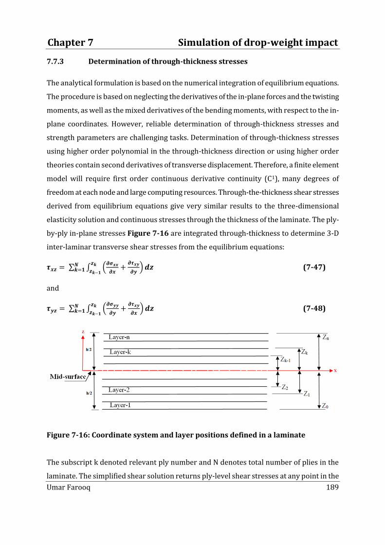
Chapter 7 Simulation of drop-weight impact
Umar Farooq 189
7.7.3 Determination of through-thickness stresses
The analytical formulation is based on the numerical integration of equilibrium equations.
The procedure is based on neglecting the derivatives of the in-plane forces and the twisting
moments, as well as the mixed derivatives of the bending moments, with respect to the in-
plane coordinates. However, reliable determination of through-thickness stresses and
strength parameters are challenging tasks. Determination of through-thickness stresses
using higher order polynomial in the through-thickness direction or using higher order
theories contain second derivatives of transverse displacement. Therefore, a finite element
model will require first order continuous derivative continuity (C1), many degrees of
freedom at each node and large computing resources. Through-the-thickness shear stresses
derived from equilibrium equations give very similar results to the three-dimensional
elasticity solution and continuous stresses through the thickness of the laminate. The ply-
by-ply in-plane stresses Figure 7-16 are integrated through-thickness to determine 3-D
inter-laminar transverse shear stresses from the equilibrium equations:
𝝉𝒙𝒛 = 𝝏𝝇𝒙𝒙
𝝏𝒙+
𝝏𝝉𝒙𝒚
𝝏𝒚
𝒛𝒌
𝒛𝒌−𝟏
𝑵𝒌=𝟏 𝒅𝒛 (7-47)
and
𝝉𝒚𝒛 = 𝝏𝝇𝒚𝒚
𝝏𝒚+
𝝏𝝉𝒙𝒚
𝝏𝒙
𝒛𝒌
𝒛𝒌−𝟏
𝑵𝒌=𝟏 𝒅𝒛 (7-48)
Figure 7-16: Coordinate system and layer positions defined in a laminate
The subscript k denoted relevant ply number and N denotes total number of plies in the
laminate. The simplified shear solution returns ply-level shear stresses at any point in the

Chapter 7 Simulation of drop-weight impact
Umar Farooq 190
laminate in global laminate coordinates. However, most failure analysis methods require
stress allowable in terms of ply local coordinates, where subscripts correspond to the ply
fibre direction. Therefore, stresses in global coordinates for any ply can be transformed
into local ply coordinates according to:
𝝉𝟏𝟑
𝝉𝟐𝟑 𝒌
= 𝒄𝒐𝒔𝜽 𝒔𝒊𝒏𝜽
−𝒔𝒊𝒏𝜽 𝒄𝒐𝒔𝜽 𝒌 𝝉𝒙𝒛
𝝉𝒚𝒛 𝒌
(7-49)
Where: θ is the ply angle (between the fibre direction and the global x-direction). The
components of the compliance matrix are determined more directly than those of the
stiffness matrix Eq. (3-8). For an orthotropic material, the compliance matrix components
in terms of the engineering constants:
𝑺𝒊=𝟏,𝟔; 𝒋=𝟏,𝟔 =
𝟏
𝑬𝟏−
𝝂𝟐𝟏
𝑬𝟐−
𝝂𝟑𝟏
𝑬𝟑𝟎 𝟎 𝟎
−𝝂𝟏𝟐
𝑬𝟏
𝟏
𝑬𝟐−
𝝂𝟑𝟐
𝑬𝟑𝟎 𝟎 𝟎
−𝝂𝟏𝟑
𝑬𝟏−
𝝂𝟐𝟑
𝑬𝟐
𝟏
𝑬𝟑𝟎 𝟎 𝟎
𝟎 𝟎 𝟎𝟏
𝑮𝟐𝟑𝟎 𝟎
𝟎 𝟎 𝟎 𝟎𝟏
𝑮𝟑𝟏𝟎
𝟎 𝟎 𝟎 𝟎 𝟎𝟏
𝑮𝟏𝟐
(7-50)
and
𝑺 = 𝑺𝟏𝟏𝑺𝟐𝟐𝑺𝟑𝟑 − 𝑺𝟏𝟏𝑺𝟐𝟑𝟐 − 𝑺𝟐𝟐𝑺𝟏𝟑
𝟐 − 𝑺𝟑𝟑𝑺𝟏𝟐𝟐 + 𝟐𝑺𝟏𝟐𝑺𝟐𝟑𝑺𝟏𝟑
The transverse normal strain for the orthotropic stress-strain relations can be obtain
𝜺𝒛𝒛 =𝟏
𝑪𝟑𝟑 𝝇𝒛𝒛 − 𝑪𝟏𝟑𝜺𝒙𝒛 − 𝑪𝟐𝟑𝜺𝒚𝒛 (7-51)
which can be used to eliminate 휀𝑧𝑧 from the stress-strain relations for the kth layer, leaving:
𝝇𝒙𝒙
𝝇𝒚𝒚
𝝉𝒚𝒛
𝝉𝒙𝒛
𝝉𝒙𝒚
𝒌
=
𝑸𝟏𝟏 𝑸𝟏𝟐 𝟎 𝟎 𝟎𝑸𝟐𝟏 𝑸𝟐𝟐 𝟎 𝟎 𝟎𝟎 𝟎 𝑸𝟒𝟒 𝟎 𝟎𝟎 𝟎 𝟎 𝑸𝟓𝟓 𝟎𝟎 𝟎 𝟎 𝟎 𝑸𝟔𝟔
𝒌 𝜺𝒙𝒙
𝜺𝒚𝒚
𝜸𝒚𝒛
𝜸𝒙𝒛
𝜸𝒙𝒚
𝒌
(7-52)
If ςzz is neglected as in classical lamination theory,

Chapter 7 Simulation of drop-weight impact
Umar Farooq 191
𝑸𝒊𝒋 = 𝑪𝒊𝒋 −
𝑪𝒊𝟑𝑪𝒋𝟑
𝑪𝟑𝟑, 𝒊𝒇 𝒊, 𝒋 = 𝟏, 𝟐
𝑪𝒊𝒋, 𝒊𝒇 𝒊, 𝒋 = 𝟒, 𝟓, 𝟔
Where: 𝑪𝟏𝟏 =𝑺𝟐𝟐𝑺𝟑𝟑−𝑺𝟐𝟑
𝟐
𝑺𝑪𝟏𝟐 =
𝑺𝟏𝟑𝑺𝟐𝟑−𝑺𝟏𝟐𝑺𝟑𝟑
𝑺𝑪𝟏𝟑 =
𝑺𝟏𝟐𝑺𝟐𝟑−𝑺𝟏𝟑𝑺𝟐𝟐
𝑺
𝑪𝟐𝟐 =𝑺𝟏𝟏𝑺𝟑𝟑−𝑺𝟏𝟑
𝟐
𝑺𝑪𝟐𝟑 =
𝑺𝟏𝟐𝑺𝟏𝟑−𝑺𝟐𝟑𝑺𝟏𝟏
𝑺𝑪𝟑𝟑 =
𝑺𝟏𝟏𝑺𝟐𝟐−𝑺𝟏𝟐𝟐
𝑺
𝑪𝟒𝟒 =𝟏
𝑺𝟒𝟒𝑪𝟒𝟒 =
𝟏
𝑺𝟒𝟒𝑪𝟓𝟓 =
𝟏
𝑺𝟓𝟓 𝑪𝟔𝟔 =
𝟏
𝑺𝟔𝟔
These stresses and strains can be used to predict the load at which failure initiates, and may
be compared with the corresponding allowable values employing common failure theories,
for a given load. In the static load-deflection models normal and transverse shearing
coupling effects are neglected. Such effects cannot be neglected in low velocity impact
models. If influence of the transverse shear stress is not taken into account advanced failure
criteria which use such stresses cannot be applied. If routine/formulation lacks with the
transverse stress values the code assigns it zero value that can lead to unrealistic
behaviour. The dynamically induced local transverse shear stresses generated from the
impact is required to be simulated in understanding the low velocity impact behaviour. The
transverse shear stresses are predicted efficiently using standard equilibrium relationships
thus allowing the predicted shear stresses to be incorporated in failure criteria. The off-axis
orientation (±θ) of layers generate shear coupling when they undergo shear deformations
because of opposite signs. Stress distributions through the thickness for the given stacking
sequences change dramatically if sequence changes. Stresses vary across the width of the
laminate, being zero over most of the central region and peaking near the edges. These
layer to layer stress variations have significant effects on performance and failure and must
be included in the investigations.
7.8 Failure theories for impacted composite laminates
Every material has certain strength, expressed in terms of stress or strain, beyond which it
fractures or fails. After this point a structural component can no longer support the loads
acting on it and fulfill the function for which it was designed. A failure criterion is applied to
hypothesize the loading response and failure of a structure. The results are utilised to

Chapter 7 Simulation of drop-weight impact
Umar Farooq 192
design structural component, calculate margin of safety, guide in material development,
and predict location of weak and strong directions. Numerous failure theories have been
proposed which combine features of the various approaches to identify the mode of failure.
All theories can be expressed in terms of the basic strength parameters referred to the
principal material axes stresses or strains, or any combination of these, causing onset of
yield or failure. The relevant and selected theories are described below.
7.8.1 Failure prediction using limits criteria
Failures in metallic materials are characterized by yield strengths. The strength parameter
criteria could be applied to validate and compare results from simplified and homogeneous
composite materials before rigorous analyses. The commonly applied failure criteria for
such materials are: maximum normal stress (Rankine), maximum shear stress (Tresca),
maximum normal strain theory (St. Venant), maximum distortional energy (von Mises)
criteria.
7.8.1.1 Maximum stress criteria (limit theory)
The maximum stress criteria are simple non-interacting failure criteria that compare each
stress component against the corresponding material ultimate strength allowable value.
The criteria are based on finding the stresses in the local axes and then using five strength
parameters to find whether a lamina has failed where each stress component is compared
to its allowable value (either tension or compression). If that ratio exceeds unity, then
failure initiation has occurred for that stress component at that material point. That is, each
component may fail independently at different load levels, and the maximum stress failure.
The failure takes on a positive value for tensile-related failures and a negative value for
compressive-related values. Shear-related failures have positive values for the failure.
7.8.1.2 Maximum strain criteria (energy conservation)
This theory is based on the maximum normal strain theory by St. Venant and the Maximum
Shear stress theory by Tresca as applied to isotropic materials. The strains applied to a

Chapter 7 Simulation of drop-weight impact
Umar Farooq 193
lamina are resolved to strains in the local axis. Failure is predicted in a lamina, if any of the
normal shearing strains in the local axes equal or exceed the corresponding ultimate strain.
Given the strains and stresses in an angle lamina the strain in the local axes can be found.
The maximum strain criteria are simple non-interacting failure criteria that compare the
strain components against the corresponding material ultimate strain allowable value for
three-dimensional problems where each strain component is compared to its allowable
value (either tension or compression). If that ratio exceeds unity, then failure initiation has
occurred for that strain component at that material point, each component may fail
independently at different load levels, and the maximum strain failure.
7.8.2 Interactive polynomial criteria
Adapting the Limits Criteria, failure theories were proposed to account anisotropy in
stiffness and strength of the composites. Interacting and quadratic criteria fit well to biaxial
loading as long as the two interacting stresses affect the same failure mechanism. When
two interacting failure mechanisms are different, such as longitudinal and transverse
failures, the quadratic criteria forces as artificially smooth transition from one failure into
the other. The widely applied failure criteria are Tsai-Hill and Tsai-Wu. The Tsai-Wu failure
criteria were selected to predict ply-by-ply failure employing the simulation generated in-
plane stress quantities. The Tsai-Wu failure polynomial is an interacting failure criterion
since all stress components are used simultaneously to determine whether a failure at a
material point has occurred or not. Identifying the mode of failure requires a different
approach for the material degradation step in the progressive failure model from that used
with the maximum stress criteria. No distinction is made between tension and compression
values for the normal stress components in evaluating the Tsai-Wu failure polynomial
terms. The shortcoming of Tsai-Hill and Tsai-Wu criteria is that they do not utilise through-
thickness stresses and could not explicitly differentiate matrix failure from fibre failure. To
include effects of through-thicknesses stresses the physical mode based failure criteria
were applied.

Chapter 7 Simulation of drop-weight impact
Umar Farooq 194
7.8.3 Mode base failure criteria
Failure criteria proposed in limit and inter-active theories are two and three-dimensional
and associated with lamina failure and do not include the out of plane stresses and they are
very effective for the application of thin structures where out-of-plane stresses are
negligible. The proposed 2D unidirectional failure criterion is composed of ‘Fibre-Fracture
Mode’ due to tensile-flexure coupling and `Quadratic Stress Criterion' for delamination
proposed in [112] has been utilised to predict failure and damage of impacted laminates
against the strength parameters given in below. The inter-active failure criterion (2-D) for
unidirectional composite lamina is based on relations for the tensile fibre mode:
If 𝝇𝟏𝟏 > 𝟎 𝒕𝒉𝒆𝒏 𝝇𝟏𝟏
𝑿𝑻 𝟐
+𝝇𝟏𝟐
𝑺𝑪≥ 𝟏 (7-53)
For the compressive fibre mode
𝝇𝟏𝟏 < 𝟎 𝒕𝒉𝒆𝒏 𝝇𝟏𝟏
𝑿𝒄 𝟐
≥ 𝟏 (7-54)
For the tensile matrix mode:
𝝇𝟐𝟐 > 𝟎𝒕𝒉𝒆𝒏 𝝇𝟐𝟐
𝒀𝑻
𝟐
+𝝇𝟏𝟐
𝑺𝑪≥ 𝟏 (7-55)
For the compressive matrix mode:
If 𝝇𝟐𝟐 < 𝟎𝒕𝒉𝒆𝒏 𝝇𝟐𝟐
𝟐𝑺𝑪 𝟐
+ 𝒀𝒄
𝟐𝑺𝑪 𝟐
− 𝟏 𝝇𝟐𝟐
𝒀𝑪+
𝝇𝟏𝟐
𝑺𝑪 𝟐
≥ 𝟏 (7-56)
Where: 𝜍11 𝑎𝑛𝑑 𝜍22are the stresses parallel and perpendicular to fibre direction, 𝜍12 is the
in-plane shear stress of the lamina, 𝑋𝑇 is the tensile strength of the fibres, 𝑋𝐶 is the
compressive strength of the fibre, 𝑌𝑇 is the tensile strength in the transverse direction of
the fibres, 𝑌𝐶 is the compressive strength in the transverse direction of the fibres, and 𝑆𝐶 is
the in-plane shear strength. However, the interactive failure criteria utilised in [112] do not
include out-of-plane stresses. Hashin in [113] proposed a general failure criterion in terms
of the stress invariants for a transversely isotropic material. The failure modes associated
with the criteria are:
Tensile fibre failure for 𝜍11 ≥ 0

Chapter 7 Simulation of drop-weight impact
Umar Farooq 195
𝝇𝟏𝟏
𝑿𝑻 𝟐
+𝝇𝟏𝟐
𝟐 +𝝇𝟏𝟑𝟐
𝑺𝟏𝟐𝟐 =
> 𝟏 𝒇𝒂𝒊𝒍𝒖𝒓𝒆≤ 𝟏 𝒏𝒐 𝒇𝒂𝒊𝒍𝒖𝒓𝒆
(7-57)
Compressive fibre failure for 𝜍11 < 0
𝝇𝟏𝟏
𝑿𝑪 𝟐
= > 𝟏 𝒇𝒂𝒊𝒍𝒖𝒓𝒆
≤ 𝟏 𝒏𝒐 𝒇𝒂𝒊𝒍𝒖𝒓𝒆 (7-58)
Tensile matrix failure for 𝜍22 + 𝜍33 > 0
𝝇𝟐𝟐+𝝇𝟑𝟑
𝒀𝑻𝟐
𝟐
+𝝇𝟐𝟑
𝟐 −𝝇𝟐𝟐𝝇𝟑𝟑
𝑺𝟐𝟑𝟐 +
𝝇𝟏𝟐𝟐 +𝝇𝟏𝟑
𝟑
𝑺𝟏𝟐𝟐 =
> 𝟏 𝒇𝒂𝒊𝒍𝒖𝒓𝒆≤ 𝟏 𝒏𝒐 𝒇𝒂𝒊𝒍𝒖𝒓𝒆
(7-59)
Compressive matrix failure for 𝜍22 + 𝜍33 < 0
𝒀𝑪
𝟐𝑺𝟐𝟑 𝟐
− 𝟏 𝝇𝟐𝟐+𝝇𝟑𝟑
𝒀𝒄 +
𝝇𝟐𝟐+𝝇𝟑𝟑 𝟐
𝟒𝑺𝟐𝟑𝟐 +
𝝇𝟐𝟑𝟐 −𝝇𝟐𝟐𝝇𝟑𝟑
𝑺𝟐𝟑𝟐 +
𝝇𝟏𝟐𝟐 +𝝇𝟏𝟑
𝟐
𝑺𝟏𝟐𝟐 =
> 1 𝒇𝒂𝒊𝒍𝒖𝒓𝒆≤ 𝟏 𝒏𝒐 𝒇𝐚𝒊𝒍𝒖𝒓𝒆
(7-60)
Inter-laminar normal stress 𝜍33 > 0
𝝇𝟑𝟑
𝒁𝑻 𝟐
= > 𝟏 𝒇𝒂𝒊𝒍𝒖𝒓𝒆
≤ 𝟏 𝒏𝒐 𝒇𝒂𝒊𝒍𝒖𝒓𝒆 (7-61)
Inter-laminar normal stress 𝜍33 < 0
𝝇𝟑𝟑
𝒁𝑪 𝟐
= > 𝟏 𝒇𝒂𝒊𝒍𝒖𝒓𝒆
≤ 𝟏 𝒏𝒐 𝒇𝒂𝒊𝒍𝒖𝒓𝒆 (7-62)
Where: 𝜍13 𝑎𝑛𝑑 𝜍23 are the out-of-plane shear stresses, 𝜍33 is the stress in the thickness
direction (z), and 𝑆𝑇 is the transverse shear strength. These failure criteria require reliable
estimates of through-thickness stresses and additional strength parameters (ZT: tensile &
ZC: compressive) and (S13 and S23) are in the transverse shear directions.
Simulation analysis carried out herein using ABAQUSTM software [82] efficiently
determines through-thickness and then utilises them in a defined failure criteria. These
stresses calculated from Eq. (7-40) and Eq. (7-49) can be used to predict the load at which
failure initiates and compared with the corresponding allowable values employing
advanced failure theories for a given load more reliably. However, efficient determination
of 3D stresses for impact on composite laminates is not possible. The procedure is based on

Chapter 7 Simulation of drop-weight impact
Umar Farooq 196
neglecting the derivatives of the in-plane forces and the twisting moments, as well as the
mixed derivatives of the bending moments, with respect to the in-plane coordinates. Here,
computer generated values at regions of high concentration of in-plane ply-by-ply stress
𝜍11 , 𝜍22 , 𝜏12 values were recorded at selected points. The recorded values for normal in-
plane axial stresses (𝜍11 𝑎𝑛𝑑 𝜍22) and in-plane shear stresses (𝜏12 𝑎𝑛𝑑 𝜏21) values were
utilised to numerically integrate ply-by-ply through-thickness stresses using Eq. (7-49).
Theses through-thickness stresses were utilised in equilibrium Eq. (7-40) to estimate ply-
by-ply through-thickness shear stresses (𝜏13 𝑎𝑛𝑑 𝜏23) using modified Simpson’s rule based
on second-order polynomial:
𝒇 𝒙 𝒅𝒕 ≈𝒉
𝟑 𝒇 𝐚 + 𝒇(𝒃) + 𝟐 𝒇 𝒙𝟐𝒌 + 𝟒 𝒇(𝒙𝟐𝒌−𝟏)
𝒏𝟐
𝒌=𝟏
𝒏𝟐 −𝟏
𝒌=𝟏
𝒃
𝒂 (7-63)
Where: the interval [a (lower limit), b (upper limit)] is split up in n sub-intervals, with n an
even number where equidistant x values are x0, x1, ..., xn, the step width being ℎ = 𝑏−𝑎
𝑛. The
method is simple and efficient to predict 3-D transverse shear stresses from a 2-D model.
These predicted and calculated stresses then can be used in failure theories to predict
possible failure modes. The failure criteria can also distinguish and separate the failure
modes.
7.9 Material properties and plan of simulations using ABAQUSTM software
7.9.1 Simulation models with sweeping meshes
Simulation models were developed to implement drop-weight impact process into
ABAQUS™ software. Commercial finite element codes are being widely used to obtain
solution of engineering and physical problem effectively and to an acceptable level of
accuracy. Built-in features of the software can be modified for specific analyses with
minimum efforts such as impact on composite laminates. The software incorporates a
variety of linear and nonlinear shell elements that could accommodate stacks of plies.
Moreover, simulations can be extended by scaling structural components. Explicit Dynamic

Chapter 7 Simulation of drop-weight impact
Umar Farooq 197
routine was chosen for this analysis. No catastrophic failures or complete penetrations
were assumed. Simulation models were developed to implement drop-weight impact
process with four distinct parts: laminate, impactor, support, and applied load. Laminate
was meshed with general purpose linear fully integrated quadrilateral conventional shell
(S4) 234 elements and reduced integration triangular conventional shell (S3R) 621
elements using two different levels of refinement. Each laminate ply is modelled with
deformable one shell element through-the-thickness which behaves according to the
continuum damage model. Fine meshes were created in regions of the model where a
correct prediction of the damage initiation load was required, such as the impact zone. The
impactors were modelled by a hardened stainless steel, meshed with fully integrated
continuum 8-node C3D8 three-dimensional (3D) linear hexahedral 708 elements. Both the
impactors have lumped masses equal to the one used in the experiments. Simulation
produced meshed (using sweeping techniques) model of symmetric 16-Ply laminate is
shown Computer generated pre-processed lay-ups of 8-Ply (un-deformed) laminate is
shown in Figure 7-17(c).
Figure 7-17: Computer generated meshed models and stack of 8-Ply laminate [4]
7.9.2 Adaptive meshing techniques
Grid adaptation meshing procedure yields an acceptable precision with the minimum
amount of computational efforts. The technique is highly useful for adaptation of various
discontinuities, interfaces, or localized large-gradient regions. Several approaches have

Chapter 7 Simulation of drop-weight impact
Umar Farooq 198
been employed for both structured and unstructured mesh adaptation, categorized into h-
methods and p-methods. The h-methods control the local mesh size in the finite element
grid by subdividing the elements when the local error estimate exceeds a user-specified
tolerance. The p-methods adapt the approximation by increasing or decreasing the local
order of polynomial basis in elements where the error in the element exceeds or falls below
a user-specified error criterion. A combination of the adaptive strategies leads to very
effective h-p methods that combine a variation in local mesh size to have the best
theoretical convergence rates. The adaptive mesh technique is incorporated in the main
analysis ABAQUSTM software. The program can start with a coarse initial mesh and compute
the field on it. Mesh can be refined based on the first coarse approximation of the field
automatically. Computational domain under nose tip was partitioned. And the adaptive
techniques were selected and implemented for unstructured grids using local refinement
frequency of 10 to 3 sweeping ratios of the grid. That increased number of S4 elements per
ply from 234 to 922. Two models were developed for comparison and verification. The
model 1 consists of impact from flat nose shape and model 2 consists of impact from round
nose shape impactors Figure 7-18(a)-(b). Impactors were meshed using the reduced
integration 8-node brick (C3D8R) 708 elements. Meshing element for laminates were full
integration linear general purpose quadrilateral shell elements and tri-angular shell
element with reduced integrations.
Figure 7-18: Computer generated impact models: a) Flat nose b) Round impactors

Chapter 7 Simulation of drop-weight impact
Umar Farooq 199
7.10 Discussion based on intra-simulation results
7.10.1 Impact of 8-Ply laminate
7.10.1.1 Impact velocity 1.7 m/s
Contour images and legend tables are shown in Figure 7-19 depicting in-plane stresses
(S11 tensile-axial; S22 tensile-lateral; and S12) for a selected top ply. Clear difference can be
seen under impact from flat and round nose profiles. The contour images depict relatively
larger damage zones under flat nose impact than those of the round nose impact. However,
larger values of predicted stress quantities from round nose impact were observed. This
suggests that round nose impactors generate larger local stresses around vicinity of the
impactors’ nose shape. However, flat nose impactor generates larger damage and stresses
spread all over the global surface of the laminate. The difference in impact induced damage
and stresses were further clarified and confirmed by contour images in direction
perpendicular to fibre and images of shear stress contours. The ply-by-ply computed in-
plane tensile, shear, and tensile-flexural stresses quantities were compared to allowable
but no failure was predicted. The in-plane stresses were recorded at specific high stress-
gradient points and numerically integrated using Eq. (6-63) to predict in-plane through-
thickness stresses.

Chapter 7 Simulation of drop-weight impact
Umar Farooq 200
Figure 7-19: Top-ply in-plane stresses Pa of 8-Ply laminate at velocity 1.7 m/s [4].
Components of coupled in-plane through-thickness stresses were compared to allowable
using Eq. (7-44) and Eq. (7-47) to predict ply level damage and failure. However, ply-by-ply
stress values were found to be negligible. The allowable coupling tensile-flexure failure
modes for flat and round impacts were negligible due to the low impact velocity range. The
in-plane through-thickness stresses were then utilised in Eq. (5-53) and (7-63) to calculate
through-thickness shear stresses using numerically integration Eq. (7-54). The components
of predicted shear stresses were put in Eq. (7-53) to Eq. (7-62) to predict ply-by-ply failure
Round nose Flat nose

Chapter 7 Simulation of drop-weight impact
Umar Farooq 201
and damage. The compared values are generally denoted as failure index. No significant
damage was seen due to impact from flat nose impact so has not been reported. The ply-by-
ply comparison of failure index in bar-chart from round nose impact shows that allowable
for ply 6 exceeds allowable limits and shows failure Figure 7-20.
Figure 7-20: Failure index based on ply-by-ply through-thickness stresses
Similarly, plies 4 and 7 both show signs of potential damage (failure index greater than 0.5).
This confirms limitations of the results obtained using load-displacement methodology.
7.10.1.2 Impact velocity 2.2 m/s
The simulation and failure processes were further performed to evaluate response of 8-Ply
laminates under flat and round nose impacts at velocity 2.2 m/s. Contour images and
legend tables depicting in-plane stresses (S11 tensile-axial; S22 tensile-lateral; and S12) for a
selected top ply are shown in Figure 7-21. The stress quantities in legend tables are higher
however, do not predict failure utilising limit theories. Hence, process of the numerical
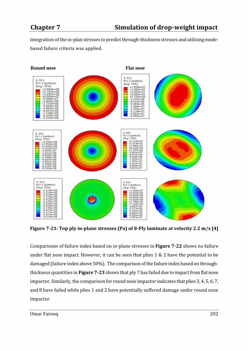
Chapter 7 Simulation of drop-weight impact
Umar Farooq 202
integration of the in-plan stresses to predict through-thickness stresses and utilising mode-
based failure criteria was applied.
Figure 7-21: Top ply in-plane stresses (Pa) of 8-Ply laminate at velocity 2.2 m/s [4]
Comparisons of failure index based on in-plane stresses in Figure 7-22 shows no failure
under flat nose impact. However, it can be seen that plies 1 & 2 have the potential to be
damaged (failure index above 50%). The comparison of the failure index based on through-
thickness quantities in Figure 7-23 shows that ply 7 has failed due to impact from flat nose
impactor. Similarly, the comparison for round nose impactor indicates that plies 3, 4, 5, 6, 7,
and 8 have failed while plies 1 and 2 have potentially suffered damage under round nose
impactor.
Round nose Flat nose

Chapter 7 Simulation of drop-weight impact
Umar Farooq 203
Figure 7-22: Failure index based on ply-by-ply through-thickness stresses
Figure 7-23: Failure index based on ply-by-ply through-thickness stresses
Drop in load-deflection curves also suggested considerable difference under flat and round
impacts. However, load-deflection results cannot be readily compared to predict status at

Chapter 7 Simulation of drop-weight impact
Umar Farooq 204
ply level. Comparisons of the results confirmed that the stress-based simulation model is
capable to predict flat and round nose impact response of relatively thin laminates. Hence,
simulations were further extended for the cases of 16-Ply and 24-Ply laminates.
7.10.2 Impact of 16-Ply laminate
The 16-Ply laminates were simulated at 3.12 m/s velocity impacts from flat and round nose
impactor to investigate their impact performance response. Contour images and legend
tables are shown in Figure 7-24 depicting in-plane stresses (S11 tensile-axial; S22 tensile-
lateral; and S12) for a selected top ply. It can be seen from the stress quantities in legend
tables that their comparisons to allowable do not predict failure utilising limit theories.
Hence, process of the numerical integration of the in-plan stresses to predict through-
thickness stresses and utilising mode-based failure criteria was applied.

Chapter 7 Simulation of drop-weight impact
Umar Farooq 205
Figure 7-24: Top ply in-plane stresses Pa of 16-Ply laminate at velocity 3.12 m/s [4]
Comparisons of the in-plane stress quantities generated from flat nose impacts predicted
no significant damage or failure. Hence, the bar-chart comparison is not reported.
Comparison from round nose impact shows Figure 7-25 that plies 1 and 2 have failed
while ply 4 also has suffered a significant damage.
Flat nose Round nose

Chapter 7 Simulation of drop-weight impact
Umar Farooq 206
Figure 7-25: Failure index based on ply-by-ply through-thickness stresses
Comparisons of the failure index based on through-thickness stress quantities generated
from flat nose impact in Figure 7-26(a) show that 7 to 14 plies have the largest shear
stress however they are not near to the levels needed to contribute to the mechanisms of
failure. While comparison from round nose impact in Figure 7-26(b) shows that plies 1
and 2 have failed while four other plies also having the potential to suffer damage.

Chapter 7 Simulation of drop-weight impact
Umar Farooq 207
a) Flat nose
b) Round nose impact
Figure 7-26: Failure index based on ply-by-ply through-thickness stresses
Chapter 7 Simulation of drop-weight impact
Umar Farooq 208
7.10.3 Impact of 24-Ply laminate
The ply-by-ply failure process was extended for 24-Ply laminates simulated at velocities
3.12 m/sand 4 m/s. Contour images and legend tables generated depicting in-plane
stresses (S11 tensile-axial; S22 tensile-lateral; and S12) for a selected top ply are shown in
Figure 7-27 and Figure 7-28 respectively. The stress quantities in legend tables are lower
hence process of numerical integration of the in-plan stresses to predict through-thickness
stresses and utilising mode-based failure criteria was applied. Components of predicted in-
plane stresses were utilised in failure criteria Eq. (6-44) to (6-47) to predict ply-by-ply
damage and failure. No significant damage was seen under flat and round nose impactors.
Hence, no comparative table or column chart is included. Similarly, comparison of through-
thickness stress components were utilised in failure and delamination criterion from Eq.
(6-48) to Eq. (6-54) to predict ply-by-ply damage and failure. No ply failure or significant
damage was observed hence no bar chart is included. Since laminates were relatively
thicker and were able to resist impacts from both the types.

Chapter 7 Simulation of drop-weight impact
Umar Farooq 209
Figure 7-27: Top ply in-plane stresses Pa of 24-Ply laminate at 3.12 m/s [4]
Round nose Flat nose

Chapter 7 Simulation of drop-weight impact
Umar Farooq 210
Figure 7-28: Top ply in-plane stresses Pa of 24-Ply laminate at velocity 4 m/s [4]
Comparison of failure index based on through-thickness stress components generated from
round nose impact simulations were utilised in failure and delamination criteria to predict
ply-by-ply damage status. Failure index in bar-chart of round nose impacts in Figure 7-29
and Figure 7-30 show no ply failure. However, plies 14 to 18 could potentially contribute
to the start of the failure process at both the impact velocities. As laminates were relatively
thicker and were able to resist impacts from both the types.
Flat nose
Round nose

Chapter 7 Simulation of drop-weight impact
Umar Farooq 211
Figure 7-29: Failure index based on ply-by-ply through-thickness stresses
Figure 7-30: Failure index based on ply-by-ply through-thickness stresses
Ratio of delaminated area in Table 7-3 produced from load-deflection test and simulation
produce images in provide knowledge about overall surface damages. All the contour
images consistently show clear difference under impact from flat and round nose profiles.
Relatively larger damage zones were produced by flat nose impact than those of the round
nose impact while larger stress quantities were produced by round nose impacts. Larger

Chapter 7 Simulation of drop-weight impact
Umar Farooq 212
local stresses are produced by the round nose impactor while larger damage spreading
stresses all over the global surface is produced by flat nose impactor.
7.11 Summary
Flat and round nose low velocity impact response of laminates with three different lay-up
stack and thickness were investigated through experimental and simulation tests. It was
observed the experimental and simulated results based on load-deflection methodology for
flat and round nose profile produced no potential damage or ply failure up to 1.7 m/s
velocity range. Ratios of delaminated areas have been consistent and in direct proportion to
velocity levels by impacts from both types of the impactors. Larger global-deflections were
produced by flat nose impact of thin laminates than those which occur from round nose
impacts.
Simulation produced 2D stresses from stress-based methodology were numerically
integrated using MATALABTM software to predict 3D stresses. The predicted 3D stress
values were utilised in mode-based and coupling failure criteria to predict ply-by-ply
damage status. Comparison of the results predicted ply level failure at 1.7 m/s velocity with
round nose impactor. Through-thickness stresses produced by flat nose impact of 24-Ply
laminates were found to be negligible compared to the stresses produced by round nose
impactors at the same velocity levels.
Comparisons of the results confirmed that the stress-based simulations are efficient and
more reliable than those based on the load-deflection experiment and simulation.

Chapter 7 Simulation of drop-weight impact
Umar Farooq 213

Chapter 8 Drop-weight impact
Umar Farooq 214
Chapter 8 Low velocity impact of composite laminates
8.1 Review
This chapter reports impact testing of the composite laminates using an instrumented
drop-tower impact machine. Laminates consisting of eight, sixteen, and twenty-four plies
impacted by flat and round nose impactors. Displacement, force, energy, and velocity
histories were recorded and plotted to approximate impact induce damage. Post-impact
non-destructive damage diagnostic techniques were applied to examine and quantify
impact induced damage. Impact generated results were compared and analysed to evaluate
response of the range of impacted laminates. Graphical surfaces and visual images
developed to interpret correlation among selected results. Common limitations of the
physical testing and post-impact testing have also been briefly described. The unknown
impact parameters were determined from estimated parameters using mathematical
formulations. The additional aim of the experimental study was to validate selected results
and establish whether simulations provide an efficient method to reduce the level of
physical testing. Discussion on comparison and validation of the results is also presented.
8.2 Carbon fibre reinforced laminates and type of impactors
The same carbon fibre composite laminates and impactors were selected as shown in
Figure 7-6. Similarly, the tests were selected from the flowchart shown in Figure 7-7.
8.2.1 Drop-weight impact test methodology
In the simple process, a mass is raised to a known height and then released to impact the
laminate. The specific operation of this type of machine creates a more realistic “real world”
scenario to obtain greater amounts of information from the impact on composites. The
same drop weight type machine was selected for testing herein that represents situations
such as accidentally falling: dropped hammer, tool (box) during fabrication or maintenance
as well as accidental hit of low speed kitchen van. Drop-weight impact analysis is a
technique that helps researchers to think through the full impact events of a proposed
change. As such, it is reliable and an essential part of the evaluation process for major

Chapter 8 Drop-weight impact
Umar Farooq 215
decisions of composites. Furthermore, it gives the ability to spot problems beforehand to
develop plans to avoid anticipated issues smoothly. The INSTRONTM drop-weight impact
tester shown in Figure 7-8 was used for the repeat of extended testing herein.
8.2.2 Impact testing plan
Since analytical analysis and computational methods alone cannot provide answers to the
problem of predicting the response of a system to low-velocity impact. Hence, it is
necessary to use empirical techniques to fill in the knowledge gaps for the real materials
and structures. The role of planned testing within the impact design methodology is crucial
to the impact design process. However, testing adds to the cost-in terms of time, money,
and personnel resources of the product development. The goal is to have a strategy which
results in minimum testing required to select the best concept. To accomplish this, the test
plan was designed to interactively support analysis activities. Test plan for the laminates
prepared based on the relevant average dimensions proposed in experimental studies in
and based on computer simulation are shown in Table 8-1.

Chapter 8 Drop-weight impact
Umar Farooq 216
Table 8-1: Impact testing plan
Laminate lay-up Average
thickness
(±0.02) mm
Test code
Velocity
(±0.2)m/s
Flat Round
8-Ply 2.4 A-1 B-1 1.7
A-2 B-2 2.2
A-3 B-3 2.2
A-4 B-4 3.2
16-Ply 4.8 C-1 D-1 3.12
C-2 D-2 3.12
C-3 D-3 3.12
C-4 D-4 3.24
24-Ply 7.2 E-1 F-1 3.74
E-2 F-2 4.3
E-3 F-3 3.74
E-4 F-4 4.3
All the laminates were impacted in accordance with the accepted American standard
testing method for measuring damage resistance of a fibre-reinforced polymer matrix
composite to a drop weight impact event (ASTM: D7136).
8.3 Non-destructive damage detection techniques
In order to study damage mechanism or failure mode, the post-impact analysis of the
impacted laminates were carried out. Different approaches exist to examine, evaluate,
characterize, and correlate impact damage through post-impact damage diagnostic
techniques. The non-destructive damage assessment techniques: Visual inspection, Eddy-
current, and Ultra-sonic C-scan are being widely used in aircraft industry. The same non-
destructive techniques were selected for this study.

Chapter 8 Drop-weight impact
Umar Farooq 217
8.3.1 Visual inspections
This is the cheapest method that involves optical inspection through an inspector’s eyes to
look for damages. Visual inspection is simple, quick and relatively inexpensive, and can
provide a good general assessment about surface damage. Generally, the central zone
(impact vicinity) of a laminate suffers damage. It is often informative to perform a
preliminary visual examination of the surfaces without sectioning or cutting the laminates.
All the impacted laminates were first examined visually to assess if there is any visible
damage. The inspector may also use special tools such as magnifying glasses, mirrors, or
bore scopes to gain access and more closely inspect the subject area. Photographs of the
typical impacted laminates with visible damage are shown in Figure 8-1. Both the front
and back surfaces show visible damages. At relatively higher energy impact, a relatively
deeper dent at front face of 8-Ply can be seen.
Figure 8-1: Image of impacted laminate: a) front and b) back surfaces

Chapter 8 Drop-weight impact
Umar Farooq 218
The visible impact damage can be observed and easily measured however, low velocity
damage is not always visible, although there can be severe underlying damage which
requires advanced damage detection techniques.
8.3.2 Eddy-current (electromagnetic induction)
The Eddy-current testing is a low cost technique that shows great potential for the
detection and characterisation of low energy impact damages. Test method is based on the
principle of electromagnetic induction. It works when an alternative current (AC) coil
carrying in proximity of the material to be tested. The magnetic field measures changes in
the impedance of an electromagnetic coil as it is scanned over a surface of conductive
material. It expands as the current rises and reduced as the current move to zero. When
this brought closely to an electrically conductive surface, the induced current would form a
circular path on the surface of materials called Eddy current. A variation in the structural
integrity of the material due to a flaw or defect will affect both the eddy currents and the
electromagnetic field as shown in Figure 8-2.
Figure 8-2: Eddy current testing
Eddy-current damage detection testing was performed for back and front faces of all the
selected impacted laminates at Electronics Department of Bolton University. The data
recorded during Eddy current tests were converted to the normalized output voltage then
MATLABTM 2010a and MS-ExcelTM 2010 software were used to plot graphs and surfaces.
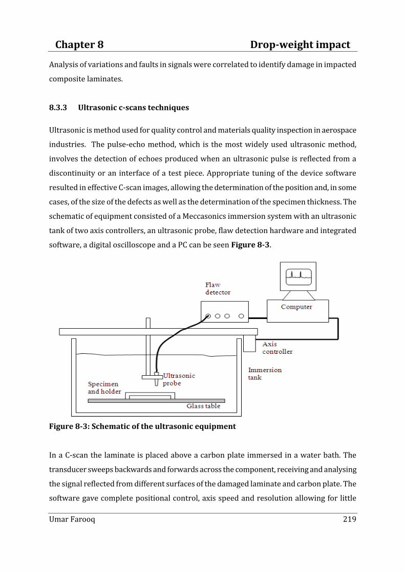
Chapter 8 Drop-weight impact
Umar Farooq 219
Analysis of variations and faults in signals were correlated to identify damage in impacted
composite laminates.
8.3.3 Ultrasonic c-scans techniques
Ultrasonic is method used for quality control and materials quality inspection in aerospace
industries. The pulse-echo method, which is the most widely used ultrasonic method,
involves the detection of echoes produced when an ultrasonic pulse is reflected from a
discontinuity or an interface of a test piece. Appropriate tuning of the device software
resulted in effective C-scan images, allowing the determination of the position and, in some
cases, of the size of the defects as well as the determination of the specimen thickness. The
schematic of equipment consisted of a Meccasonics immersion system with an ultrasonic
tank of two axis controllers, an ultrasonic probe, flaw detection hardware and integrated
software, a digital oscilloscope and a PC can be seen Figure 8-3.
Figure 8-3: Schematic of the ultrasonic equipment
In a C-scan the laminate is placed above a carbon plate immersed in a water bath. The
transducer sweeps backwards and forwards across the component, receiving and analysing
the signal reflected from different surfaces of the damaged laminate and carbon plate. The
software gave complete positional control, axis speed and resolution allowing for little
Chapter 8 Drop-weight impact
Umar Farooq 220
intervention. A pulse echo method was employed using the carbon plate as the reflective
medium. Laminates were cleaned to remove any dirt or residue and placed in a holder
slightly raised from the carbon bed. The limits of the scan are entered into the software and
the zero point indicated. The C-scan testing for all the selected laminates was carried out at
Composites’ Certification Laboratories (based at the Manchester University).
8.4 Comparison of results
8.4.1 Damage assessment of 8-Ply laminates
To investigate influence from the flat and round nose impacts further, comparisons were
also carried out against post-test experimentally generated C-scanned images. The C-scan
images show negligible damage on both the laminate surfaces as shown in Figure 7-9
which confirms no major damage has incurred to the laminates. The post-impact,
simulation generated were plotted plots obtained using MATLABTM software as shown in
Figure 7-11. It is obvious from comparison of the front and back face surfaces that there is
no major damage incurred to the laminates and no difference from the images can be seen.
The C-scan images diameters vary: 16-20 mm and the corresponding surface generated
from Eddy-current data for damage zone diameter vary: 10-18 mm of the 8-Plylaminates
impacted by round and flat nose impactors at 2.4m/s velocity are shown in Figure 8-4. The
scanned images obtained from flat nose impact and corresponding front and back surfaces
show larger damage sizes when compared to the results from generated from round nose
impact. The damage factor in surfaces indicates impedance increase up to 37% depth of the
laminate thickness. This support the load-deflection results that the larger
damage/delaminated areas area created under flat nose impactors.

Chapter 8 Drop-weight impact
Umar Farooq 221
Figure 8-4: C-scan images and Eddy-current surface
The scanned images and surfaces were compared to simulated results obtained from 8-Ply
symmetric laminates impacted by flat nose and round nose impacts shown in Figure 8-5.
The flat nose impact damage corresponding to front and back surfaces show larger damage
sizes when compared to the results from generated from round nose impact. This support
the load-deflection results that the larger damage/delaminated areas are created under flat
nose impactors. Simulation produced images of tensile stresses from ply 1 to 4 show larger
damage zones under flat nose impactor. However, stresses quantities under round nose
impactors are higher. Such trend indicate that damage created by round nose impact is
local while damage created by flat nose distributed and global.
20mm 16mm

Chapter 8 Drop-weight impact
Umar Farooq 222
Figure 8-5: Simulated images and legend tables from ABAQUSTM software
Another C-scan damage zone diameters vary: 11-38 mm and images and Eddy-current
surfaces damage zone diameters vary: 11-22 mm in comparison as shown in Figure 8-6.
The 8-Ply laminates were impacted at 3.2m/s velocity (relatively higher) by round and flat
nose impactors. Delamination propagation continued throughout the thickness of the
laminate without full penetration of the back surface. The scans images indicate the similar
higher damage pattern in proportion to impact energy for Fibredux 914C-833-40 laminates.
Graphs for flat nose impactor have also shown larger damage for laminates (Fibredux
914C-833-40) impacted by relatively larger energy impacts. Similar response cases can be
seen in the load-placement curve during the rebound that did not match during loading.

Chapter 8 Drop-weight impact
Umar Farooq 223
Figure 8-6: C-scan images and Eddy-current surface
The C-scan images (damage zone diameters vary: 6-36 mm) and Eddy-current surfaces
(damage zone diameters vary: 9-26 mm) of the 16-Ply laminates impacted by round nose
impactor by relatively higher energy impact are shown in Figure 8-7. The scans images
indicate distributed and higher damage level as compared to the flat nose impact images.
While Eddy-current surfaces show higher damage at their front and back faces than that of
round nose impactors. The different damage pattern shown under both the nose tips
confirm limitations of the damage diagnostic techniques. As laminates are relatively thick
so through-thickness damage and internal delamination propagation continued throughout
the thickness and these tests cannot pick the internal damage. Delamination propagation
also continued throughout the thickness of the laminate without full penetration of the
back surface. The scans indicate the severity of the delamination as dark gray central zone
under round nose impactor.
11mm
38mm

Chapter 8 Drop-weight impact
Umar Farooq 224
8.4.2 Damage assessment of 16-Plylaminates
Figure 8-7: C-scan images and Eddy-current surface
To clarify the reverse trends shown by C-scan (damage zone diameters vary: 18-69 mm)
and Eddy-current surfaces (damage zone diameters vary: 11-78 mm) test another
comparison is shown in Figure 8-8 with slightly increased velocity (3.74 m/s). It can be
seen from the figure that images and surfaces the damage inflected by round nose ruptures
the laminates under impactor’s nose tip. The damage due to flat nose impact is around the
impacted nose tip and distributed around its surrounding. The scanned images and
surfaces indicate distributed and higher damage level due to flat nose impact than round
nose impact. The Eddy-current surfaces also show higher damage at their front and back
faces than that of round nose impactors.
6mm
36mm

Chapter 8 Drop-weight impact
Umar Farooq 225
Figure 8-8: C-scan images and Eddy-current surface
Simulation produced results for 16-Ply laminates impacted by flat and round nose
impactors are shown in Figure 8-9. The bottom most 16th ply was selected to compare
shear stresses. It can be seen stresses under round nose impact are higher however damage
area under flat nose is larger. The results corroborate the experimental as well as
simulation produced 8-Ply laminate results.
18mm 69mm

Chapter 8 Drop-weight impact
Umar Farooq 226
Figure 8-9: Simulated images and legend tables from ABAQUSTM software
To clarify the trends shown by C-scan (damage zone diameters vary: 16-42 mm) and Eddy-
current (damage zone diameters vary: 15-68 mm) test another comparison is shown in
Figure 8-10 with slightly increased velocity (3.74 m/s). It can be seen from the figure that
images and surfaces the damage inflected by round nose ruptures the laminates under
impactor’s nose tip. The damage due to flat nose impact is around the impacted nose tip
and distributed around its surrounding. The scanned images and surfaces indicate
distributed and higher damage level due to flat nose impact than round nose impact. The
Eddy-current surfaces also show higher damage at their front and back faces than that of
round nose impactors.
8.4.3 Damage assessment of 24-Plylaminates
-
Figure 8-10: C-scan images and Eddy-current surface
16mm 42mm
17mm
15mm
26mm
68mm

Chapter 8 Drop-weight impact
Umar Farooq 227
To clarify the mixed trends comparison of the C-scan images (damage zone diameters vary:
38-68 mm) and surfaces (damage zone diameters vary: 18-88 mm) from Eddy-current test
is shown in Figure 8-11 with increased velocity of 4.2 m/s. It can be seen from the figure
that images and surfaces the damage inflected by round nose ruptures the laminates under
impactor’s nose tip. The damage due to flat nose impact also penetrates in top plies rupture
type trace can be seen. Moreover, damage under flat nose tip is more distributed around its
surrounding. The scanned images and surfaces indicate distributed and higher damage
level due to flat nose impact than round nose impact. The Eddy-current surfaces also show
higher damage at their front and back faces than that of round nose impactors.
Figure 8-11: C-scan images and Eddy-current surface
Simulation produced results for 24-Ply laminates impacted by flat and round nose
impactors are shown in Figure 8-12. The middle 12th ply was selected to compare damage
38mm 68mm
18mm
78mm
28mm
88mm

Chapter 8 Drop-weight impact
Umar Farooq 228
zone and lateral stresses. It can be seen that the quantities of stresses under round nose
impact are higher however damage area under flat nose is larger. The results consistent
trends confirmed the experimental as well as simulation produced 8-Ply and 16-Ply
laminates results.
Figure 8-12: Simulated images and legend tables from ABAQUSTM software
8.4.4 Prediction of impact induced damage area
Since delaminations are linked from ply to ply by matrix cracks running along the fibres
forming a double helix of delaminations switching direction at the (non-delaminated)
middle layer. To clarify comparisons of the damage/delaminated zones generated due to
impacts the surfaces and images areas representing the damage zones are approximated.
The geometry of delamination defines approximate boundary between the damage and
undamaged portion of the laminate (necessary to calculate total delamination area) which
allows the prediction of the energy released per unit area of delamination once dissipated
energy is known. A set of selected images of 8-, 16-, and 24-Ply laminates is given in below
to correlate impact damage areas. The scanned areas were correlated against reduction in
stiffness parameters to predict overall damage percentage. Measured deflections were used
as the independent variable to compare against the damaged areas and found within
acceptable range (±12%). Moreover, comparisons from damage areas in C-scanned images
correlated to the damage areas diameter 4-50 mm represented by surfaces generated from
Eddy-current tests average surfaces diameter varying 10-70 mm. It was pre-assumed that
peaks relate to through the thickness damages. Comparisons of the peak heights in Figure

Chapter 8 Drop-weight impact
Umar Farooq 229
8-10 are also in acceptable range at the both front and back surfaces of the corresponding
laminates Figure 8-13.
Figure 8-13: Comparison of 24-Plylaminate C-scan and Eddy-current images.
The damaged area for the IM7/8552 is approximately 695 mm2, which equates to 3.9% of
the laminate total area and 8.9% of the clamped test area. The average damaged area for
the Fibredux 914C-833-40 laminate was determined as 8.01% of the clamped area. The
Table 8-2 shows a comparison of the damage area percentage produced by the round and
flat impactors in some of the tests. The determined damage and delaminated areas for the
laminates are compared below.
4mm
24m
m
50m
m
6mm 14m
m
8mm 44m
m
54m
m 84m
m

Chapter 8 Drop-weight impact
Umar Farooq 230
Table 8-2: Drop-weight impacted laminate against damage zone
Laminate Test code
Velocity
(±0.2)m/s
Damaged area (%)
Flat Round Flat Round
8-Ply A-1 B-1 1.7 0.5 0.5
A-2 B-2 2.2 6.5 6.5
A-3 B-3 2.2 7.2 6.5
A-4 B-4 3.2 10 8.12
16-Ply C-1 D-1 3.12 20.88 15
C-2 D-2 3.12 19.76 14.94
C-3 D-3 3.12 21.1 16
C-4 D-4 3.24 23.24 16.8
24-Ply E-1 F-1 3.74 6.6 12.3
E-2 F-2 3.74 7.5 13.9
E-3 F-3 4.2 20.9 21.8
E-4 F-4 4.2 21.24 20.9
The tabular results show that the damage pattern is consistent for all the thickness. It was
found that deformation areas of laminates impacted with low velocity remains below 2% of
the clamped part. Laminates impacted with relatively higher velocities (up to 4.2 m/s)
produced increased damaged areas of 20% believe to be delamination dominated. Results
caused strength and stiffness losses from 2% to 5% under low velocity impacts. The
damage state may differ according to increased velocity impacts reducing strength and
stiffness from 10% to 20% (±0.5) with obvious surface damage.

Chapter 8 Drop-weight impact
Umar Farooq 231
8.4.5 Laminates of different material properties
Impact test results from IM7/8552 made laminates subjected to hemi-spherical and flat
nose shape impacts were available. Selected test results of Fibredux 914C-833-40 made
laminates subjected to round and flat nose impactors were compared to verify selected
results and response patterns of the impacted laminates. The comparisons proved to be
very useful in studying overall view of the interpretation of the impact response.
8.4.5.1 8-Ply laminate impacted at velocity 1.7 m/s
The C-scan images show only scattered small marks (isolated fragments) on the front
where the impactor hit and only slightly more visible damage on the backside and still no
visible cracks. There was no crack on the topside or backside crack in the fibre direction on
all laminates. The laminates exhibited far less damage due to the lower impact energy level.
Visual and ultrasonic inspection confirmed that the laminates suffered only small
indentations on the impact surfaces, which is attributed to the initial portion of the
response. No change in normal attenuation of the ultrasonic signal recorded for both the
laminates from IM7/8552 and Fibredux 914C-833-40 as shown with the clear scan in
Figure 7-9 (a) & (b) due to relatively low velocity range.
8.4.5.2 16-Ply laminate impacted at velocity 3.12 m/s
The responses of laminate impacted at 3.12 m/s velocity round nose impact. The C-scan
images show matrix cracking, de-lamination, fibre breakage, low inter-laminar shear
strength, and de-bonding as the dominant internal damage/failure mechanisms. Similar
pattern is shown on both the images of different types of materials and confirmed by the
ultrasonic Figure 8-14(a) and Figure 8-14(b) that not only had indentation damage
occurred on the impact surface but also internal damage in the form of de-lamination. In
the figure a major change in the attenuation of the ultrasonic signal is recorded as an
almost circular feature in the centre of the laminate. No other damage was visible after
inspection and so it was concluded that the change in response was attributed to
delamination initiation and propagation. The results support the prediction that as the
impactor nose becomes flat the internal damage area increases.

Chapter 8 Drop-weight impact
Umar Farooq 232
a) IM7/8552 laminate b) Fibredux 914C-833-40 laminate
Figure 8-14: C-scan image of 8 J impact using the round impactor
8.4.5.3 24-Ply laminate impact energy: 20 J, 30 J, and 50 J
In Figure 8-15(a) images are presented (plots from IM7/8552 are not available) for gross
damage area by 20 J, 30 J and 50 J energy impact by round nose impactor used in the
creation of the damage in 24-Ply IM7/8552 Figure 8-6 and Fibredux 914C-833-40 made
laminates. The C-scan images of both types of laminates impacted show increasing damage
trend with increased impact energy levels.
Figure 8-15: C-scan images using flat impactor
8mm 9mm
8mm 18mm 16mm
10mm 15mm 20mm

Chapter 8 Drop-weight impact
Umar Farooq 233
8.5 Limitations associated with testing and non-destructive techniques
A major issue of the Ultrasonic C-scan is the large amount of accumulated data to have a
sufficient resolution to detect small cracks within a large scanned region. However,
conventional C-scan machine produces 2D scan plots where multi-plane delaminations are
projected on a single plane. Different approaches exist to: examine, evaluate, characterise,
and correlate impact damage through post-impact analyses of the tested laminate and
generated data. Most of the reported non-destructive techniques to collaborate in damage
diagnostics and failure status are: visual inspections, multi-disciplinary field ultra-sonic C-
scans, and Eddy-current testing of the impacted laminates and post-processing of the test
generated data. Different approaches exist to: examine, evaluate, characterise, and
correlate impact damage through post-impact analyses of the tested laminate and
generated data. The techniques produce a planar indication of the type and extent of
damage to detect certain kinds of defects, monitor the distribution, extent, nature, and
progression of impact damage. It causes no major damage during testing the laminate.
Tested laminate can be used a number of times or other test can be performed on the same
laminate. Comparative Ultrasonic analysis of damage in composites under static
indentation and low-velocity impact is reported. The impact testing, data logging, and
damage assessment techniques have limitations[1]. Performance evaluation of structural
parts depends on quantifying and locating pattern of the delamination and internal damage
within the impacted laminates. Continuing with the base-line (bench-marked) results
obtained to validate test produced results show limitations. Deviations in load-deflection
graphs of thick laminates (16 and 24-Ply) as shown in Figure 8-16 due mechanical
characteristics, experimental and tester manufacturing limitations turn out to be obviously
detectable. Load-deflection curves turned into certain lines after and become straight and
do not show any sign of variation. To further investigate and confirm the data results the
experimentally estimated parameters need to be used in mathematical formulations to
determined extended impact parameters with reduced testing.

Chapter 8 Drop-weight impact
Umar Farooq 234
Figure 8-16: Load-time history of flat and round nose impacts.
8.6 Theoretical determination of impact parameters
There are many theoretical aspects that must be considered for the extended interpretation
of experimentally produced test data. The level of the impact energy or momentum is
changed by varying the drop height of the impactor. This has the effect of changing both the
impact energy and the impact velocity simultaneously. The analytical impact parameters
are useful tool to get fast predictive results for an unknown parameter from mathematical
relations using known parameters for a given impact configuration. These models are
usually developed to predict the response of the system until damage onset, which is
sufficient to compare different impact cases with different values of the governing
parameters.All recorded data generated from the impact tests were used to calculate other
unknown values. The main constraints on the theoretical formulations were that the all
deformations were in the elastic region. The use of test generated data in place of more
costly impact testing have been utilised to calculate other unknown parameters. From the
experimentally measured/known parameters such as load, velocity, displacement, energy
other theoretical aspects were considered for any possible relations. The parameters
estimated with experiment are used to determine the other possible parameters useful to
correlate and estimate impact damage and damage mechanism.

Chapter 8 Drop-weight impact
Umar Farooq 235
8.6.1 Parameters that affect the impact response
The parameters that affect the impact response can be classified into three different
groups: structural parameters, impactor parameters and environmental conditions.
Parameters like shape, thickness, size, material properties, ply stacking sequence, and
boundary conditions are categorized as structural parameters. Impactor parameters
comprise shape, diameter, material properties, weight, angle of incidence and impact
velocity. Davies [18] found that under the same impact energy, the structural parameters,
like shape, size and boundary conditions affect the impact response significantly. For
example, a small plate is stiffer than a large plate which results in a larger impact force on
the small plate. So, the relationship between impact force and damage area was used
instead of that between impact energy and damage area as that means there was no need to
consider plate size and other effects. The research results paved the way that a small piece
of test specimen can be used to simulate impact damage in a large in-service structure
when the same impact force was employed. At the same time impactor geometry severely
affects the impact damage of a plate [16]. Theoretically determined impact parameters can
be correlated to:
a) Impact energy – kinetic energy of the impactor;
b) Peak force – maximum force recorded during the impact event;
c) Critical force – threshold force for onset of delamination;
d) Critical energy – impact energy analogous to critical force;
e) Dissipated energy – energy absorbed in damage initiation and propagation
8.6.2 Parameters determined from impact test generated data
8.6.2.1 Forces, mass and acceleration
Acceleration (a) in free fall can be measured directly and weight can be measured
independently by the deflection of a spring. Forces (F) generally vary during an impact but
masses m remains constant. Newton’s second law of motion says
𝑭 = 𝒎𝒂 (8-1)

Chapter 8 Drop-weight impact
Umar Farooq 236
If mass of the impactor is to vary, keeping the velocity constant the following parameters
can be calculated using the Newton law:
𝑭 = 𝒎𝒈 − 𝒇 = 𝒎𝒅𝒗
𝒅𝒕 (8-2)
𝒗 = 𝒗𝟎 + 𝒈𝒕 −𝟏
𝒎 𝒇𝒅𝒕
𝒕
𝟎 (8-3)
𝒙 = 𝒗𝟎𝒕 +𝟏
𝟐𝒈𝒕𝟐 −
𝟏
𝒎 𝒇𝒅𝒕
𝒕
𝟎
𝒕
𝟎 (8-4)
Multiplying Eq. (3) by 𝑓𝑑𝑡𝑡
0
𝑬 = 𝒗𝟎 𝒇𝒅𝒕𝒕
𝟎+ 𝒈 𝒇𝒕𝒅𝒕
𝒕
𝟎−
𝟏
𝒎 𝒇𝒅𝒕
𝒕
𝟎 𝟐
(8-5)
The impact duration t can also be determined from Eq. (8-4).
8.6.2.2 Energy balances (virtual work and d’Alembert’s principle)
To consider a work which a force would do if it were to move through a small displacement
𝛿𝑥 is known as virtual work and hypothetical displacement 𝛿𝑥 is known as the virtual
displacement. Work done is defined ass force multiplied by displacement
𝑾 = 𝑭 𝒅𝒙 (8-6)
D’Alembert’s principle can be obtained by multiplying each side of Eq. (8-1), in the limit
𝑭𝒅𝒙 = 𝒎𝒂 𝒅𝒙 (8-7)
Replacing acceleration by the approximate velocity in Eq. (8-7) gives
𝑭𝒅𝒙 = 𝒎𝒗 𝒅𝒗
𝒅𝒙𝒅𝒙
= 𝒎𝒗 𝒅𝒗 (8-8)
The Eq. (8-8) can be used for both actual and virtual work. The work done equals the
energy released which is more convenient to relate the work done to the absorbed energy.
For potential energy V this relationship can be expressed as 𝛿𝑊 = 𝛿𝑉. From Eq. (8-6) the
relation can be expressed as
𝑭 = −𝒅𝑽
𝒅𝒙 (8-9)

Chapter 8 Drop-weight impact
Umar Farooq 237
Kinetic energy is possessed by a mass as a result of its velocity, and it is equals the work
needed to bring the mass up to this velocity or done by the mass if it loses its velocity. The
relationship can be derived from D’Alembert’s principle by integration both sides
𝑭𝒅𝒙𝒙𝟐
𝒙𝟏= 𝒎𝒗𝒅𝒗
𝒗𝒇
𝒗𝟎 (8-10)
As with potential energy, it is convenient to relate the work done to the kinetic energy T
absorbed in the moving body (𝛿𝑊 = −𝛿𝑇). This can be expressed as
𝑭 = −𝒅𝑻
𝒅𝒙
𝑭𝒅𝒙𝒙𝟐
𝒙𝟏= 𝒅𝑻
𝑻𝟐
𝑻𝟏 (8-11)
8.6.2.3 Energy absorbed by target
The velocity (vo) at the impact point allows the forces generated during test together with
energy absorption and deflection. Typical load-time curves recorded by the devices are
obtained to estimate the energy absorbed by target prior to failure resulting from impact
load (or high strain rate). The initial rise in the load-time curves corresponds to the fracture
initiation phase. In some cases local peak is recorded due to matrix cracking while
maximum load corresponds to fibre fracture. The area under the load-time curve is called
impulse and expressed as
𝑷𝒅𝒕 (8-12)
The total energy absorbed during the impact is
𝑬 = 𝑷𝒗𝒅𝒕𝒕𝒇𝒕𝟎
(8-13)
Where P is the instantaneous load and v is the instantaneous velocity recorded during
impact, t0 is the time of initial impact, usually taken as zero, and tf is the time for completion
of penetration. An apparent energy can be defined as
𝑬 = 𝒗𝟎 𝑷𝒅𝒕𝒕𝒇𝒕𝟎
(8-14)
A close approximation to the actual energy can be obtained by replacing the instantaneous
velocity v0 with the average velocity during penetration, 𝑣 as
Chapter 8 Drop-weight impact
Umar Farooq 238
𝑬 = 𝒗 𝑷𝒅𝒕𝒕𝒇𝒕𝟎
(8-15)
It is important that reliable and accurate method for measuring the velocity at contact is
employed because this parameter is required for the calculations of displacement and
energy. A useful feature of the moment is that it is always conserved. Impulse-moment
balances are used mainly in situations in which the duration of the forces is so short that no
significant displacement occurs before it is over. Using the relation between impulse, 𝐹 𝑑𝑡,
and momentum, 𝑚 𝑣0 − 𝑣𝑓 and approximating the average velocity as 𝑣0+𝑣𝑓
2, the
average velocity in terms of the initial velocity can be obtained by
𝑰 = 𝑭𝒅𝒕𝒕
𝟎= 𝒎 𝒗𝟎 − 𝒗𝒇 as
𝒎𝒗𝒇 = 𝒎𝒗𝟎 − 𝑭𝒅𝒕𝒕
𝟎 (8-16)
multiplying Eq. (8-16) by 𝑣0 gives
𝒎𝒗𝒇𝒗𝟎 = 𝒎𝒗𝟎𝒗𝟎 − 𝒗𝟎 𝑭𝒅𝒕𝒕
𝟎 (8-17)
or
𝒗𝒇𝒎𝒗𝟎
𝟐
𝒗 𝟎= 𝒎𝒗𝟎
𝟐 − 𝑬𝒂 or
𝒗𝒇𝟐𝑬𝟎
𝒗 𝟎= 𝟐𝑬𝟎 − 𝑬𝒂 (8-18)
The average velocity can be written as
𝒗 = 𝒗𝟎 𝟏 −𝑬𝒂
𝟒𝑬𝟎 (8-19)
The max energy available during impact of the tup as it penetrates the target in terms of
kinetic energy just prior to impact and the measured impact energy. Combining Eq. (8-15)
and (8-19) give
𝑬 = 𝐄𝒂 𝟏 −𝑬𝒂
𝟒𝑬𝟎 (8-20)
From experimental measurements and using the kinetic and elastic energies the absorbed
energy can be calculated. This leads to correlate the impact energy transferred from the
impactor to the target and absorbed by the each failure mechanisms of the fraction of
impact energy. The experimental impact force measured during the impact event makes

Chapter 8 Drop-weight impact
Umar Farooq 239
possible to evaluate the impact energy, which reaches the target as well as absorbed energy
and the elastic energy. The contact force 𝐹 𝑡 during the impact load depends on the
impactor mass m and velocity v. Initial impactor velocity 𝑣0 depends on the free fall
acceleration g and downfall height h:
𝒗𝟎 = 𝟐𝒈𝒉 (8-21)
Impactor instantaneous velocity v and displacement s as the time functions are determined
by integrating the impact force in time-domain as shown below:
𝒗 𝒕 = 𝒗𝟎 − 𝟏
𝒎 𝑭 𝒕 𝒅𝒕
𝒕
𝟎 (8-22)
𝒔 𝒕 = 𝒗𝟎 − 𝟏
𝒎 𝑭 𝒕 𝒅𝒕
𝒕
𝟎 𝒅𝒕
𝒕
𝟎 (8-23)
After the impact, the impactor velocity gradually decreases as the laminate absorbs the
impact kinetic energy equal to:
𝑬𝒊𝒎𝒑 = 𝟏
𝟐𝒎𝒗𝟐 (8-24)
The absorbed energy 𝐸𝑎𝑏 is function of time that can be determined using Eq. (8-22):
𝑬𝒂𝒃 𝒕 =𝟏
𝟐𝒎𝒗𝟎
𝟐 −𝟏
𝟐𝒎 𝒗𝟎 −
𝟏
𝒎 𝑭 𝒕 𝒅𝒕
𝒕
𝟎 𝟐
(8-25)
Peak force can be determined when impact event is modelled as a single degree of freedom
spring mass damper system based upon the assumption that target mass is negligible and
the target and impactor move together follow:
𝒎𝒙 + 𝒌𝒙 = 𝟎 (8-26)
with the general solution
𝒙 = 𝑨𝒔𝒊𝒏 𝒌
𝒎𝒕 + 𝑩𝒄𝒐𝒔
𝒌
𝒎𝒕 (8-27)
Using the boundary conditions 𝑥 0 𝑉 𝑎𝑛𝑑 𝑥 0 = 0 Eq. (8-27) yields wave amplitude as
𝒙 = 𝑽
𝒌
𝒎
𝒔𝒊𝒏 𝐤
𝒎𝒕 (8-28)
By assuming a linear elastic response (very simple case) the peak force data can be fitted by
the empirical power law curve whereby
𝑷𝒑𝒆𝒂𝒌 = 𝟐𝒌𝑬𝒊𝒎𝒑 (8-29)
By subtracting the dissipated energy from the total impactor kinetic energy a closer
estimate of the actual peak force can be obtained. However, direct comparison of the ratio

Chapter 8 Drop-weight impact
Umar Farooq 240
of contact duration and strength retention curves is required to provide validation of the
concept to determine applicability of such a curve to composite materials testing. Time
period can be obtained from the relation:
𝒕 = 𝝅 𝒎
𝒌 (8-30)
The impact velocity can be determined from energy relations: assuming the absorbed
energy, change in the strain energy ∆𝑈 is equal to the change in kinetic energy∆𝐸𝑖𝑚𝑝 . At
contact, the change in strain energy and kinetic energy is presented as
∆𝑼 = 𝑭. 𝑽 𝒅𝒕𝒕𝒏+∆𝒕
𝒕𝒏 (8-31)
∆𝑬𝒊𝒎𝒑 =𝟏
𝟐𝒎 𝑽𝒏
𝟐 − 𝑽𝒏+𝟏𝟐 (8-32)
Solving Eq. (8-31) and (8-32), the impact velocity 𝑉𝑛+1was obtained as
𝑽𝒏+𝟏 = 𝑽𝒏𝟐 −
𝟐.𝑭.𝑽𝒏∆𝒕
𝒎 (8-33)
After receiving the velocity data, the change of the strain energy was automatically
calculated with velocity, impact force, and impact time. The experimental impact force
measured during the impact event makes possible to evaluate the impact energy, which
reaches the target as well as absorbed energy and the elastic energy. The contact force
𝐹 𝑡 during the impact load depends on the impactor mass m and velocity v.
Example 8.1: A typical example of the use of impulse force calculation. To estimate the
average impact force between an impactor at 5 m/s hits a plate at 1 m distance of 5Kg mass.
Solution
Impulse 𝐼 = 𝑭𝒂𝒗𝒆𝒓𝒂𝒈𝒆𝜟𝒕 = 𝒎𝜟𝒗
The impact duration can be calculated from the characteristic length of the plate as:
𝜟𝒕 =𝟏
𝜟𝒗=
𝟏
𝟓= 𝟎. 𝟐 𝒔
Force can be calculated from impulse as
𝑭 = 𝒎𝜟𝒗
𝜟𝒕= 𝟓 ∗ (
𝟓
𝟎.𝟐) = 125 N

Chapter 8 Drop-weight impact
Umar Farooq 241
Example 8.2: Calculating the peak force when a 5 Kg mass is dropped from 1.0 m height on
to a 2.4 mm thick circular plate having a diameter of 100 mm.
Solution:
First tensile stress is calculated from area and force:
Area of the plate is 𝐴 = 𝜋 𝟓𝟎
𝟐
2
= 1964.3 𝑚𝑚2
If F is the maximum tensile force produced then stress is 𝜍 =𝐹
1964.3 and
maximum elongation is ∆𝛿 = 휀 𝑥 𝑙 = 𝜍
𝐸𝑥 𝑙 =
𝐹 𝑥 2.4
48∗(1964.3)= 0.0003 𝐹𝑚𝑚
Now loss of PE = Gain of SE
𝑤 ℎ + ∆𝛿 =1
2𝐹𝑥∆𝛿 ⇒ 5 𝑥 9.81 𝑥 1000 + 0.0003𝐹 =
1
2𝐹𝑥 0.0003𝐹
⇒ 50000 + 0.015𝐹 − 0.00015𝐹2 ⇒ 𝑇ℎ𝑒 𝑝𝑒𝑎𝑘 𝑓𝑜𝑟𝑐𝑒 𝑭 = 𝟗 𝑲𝑵
Once impulse force known the maximum energy of the tub can be determined. The total
energy absorbed during the impact duration 𝑭𝒗𝒅𝒕𝒕𝒇𝒕𝟎
where t0 is the time of initial impact,
usually taken as zero, and tf is the time for completion of penetration.
8.6.2.4 Determination of contact duration
Contact duration can to be determined by considering impact induced damage/indentation.
During impact testing the presence of harmonic oscillations potentially make identification
of the onset of damage difficult. Thus, without damage, the contact time for any initial
impact velocity is independent of drop height and the impactor free-fall velocity. With a
loss in stiffness, the contact time increases with a reduction of k. The contact duration is
then expresses with half the period for free vibrations of a single degree of freedom system
of Eq. (8-30) with stiffness k and mass m. Since the contact force is proportional to the
deflection of the impactor or laminate, the force and deflection curve differ only by the
proportionality constant, k. Hence the constant k may be determined experimentally from
curves. Thus, with a decrease in k, the duration decrease, and increases as mass increases.
The arbitrary contact duration can be determined from impact induced indentation
(damage). During impact testing the presence of harmonic oscillations potentially make
identification of the onset of damage difficult. Thus, without damage, the contact time for

Chapter 8 Drop-weight impact
Umar Farooq 242
any initial impact velocity is independent of drop height and the impactor free-fall velocity.
With a loss in stiffness, the contact time increases with a reduction of k. The contact
duration is then expresses with half the period for free vibrations of a single degree of
freedom system of Eq. (8-30) with stiffness k and mass m. Since the contact force is
proportional to the deflection of the impactor or laminate, the force and deflection curve
differ only by the proportionality constant, k. Hence the constant k may be determined
experimentally from curves. Thus, with a decrease in k, the duration decrease, and
increases as mass increases. An arbitrary time Tc during impact can be determined from
energy balance:
𝟏
𝟐𝒎𝒗𝟐 =
𝟏
𝟐𝒎𝜶 𝟐 +
𝟐
𝟓𝑲𝜶
𝟓𝟐 (8-34)
Separating (𝜶 = 𝝏𝜶
𝝏𝑻𝐜
) the variable Tc the Eq. (8-34) may be written as:
𝒅𝑻𝒄 = 𝒅𝜶 𝒗𝟐 −𝟒𝑲
𝟓𝒎𝜶
𝟓𝟐
−𝟏𝟐
(8-35)
The contact duration is double the time needed to reach the maximum indentation:
𝑻𝒄 = 𝟐 𝒗𝟐 −𝟒𝑲
𝟓𝒎𝜶
𝟓𝟐
−𝟏𝟐
𝜶𝒎𝒂𝒙
𝟎
𝒅𝜶 (8-36)
With the change of variable
𝒙 =𝜶
𝜶𝒎𝒂𝒙= 𝜶
𝟓𝒎𝒗𝟐
𝟒𝑲 𝟐
𝟓
(8-37)
The Eq. (16) may be written as:
𝑻𝒄 = 𝟐𝜶𝒎𝒂𝒙𝒗−𝟏 𝟏 − 𝒙
𝟓𝟐 −
𝟏𝟐 𝒅𝒙 = 𝟐. 𝟗𝟒 𝜶𝒎𝒂𝒙𝒗
−𝟏𝟏
𝟎 (8-38)
From the load-deflection relation the maximum displacement can be calculated using
contact law under concentrated load 100 N at center of the plate: 2.53 𝑥 10−4m. Typically,
at 3 m/s velocity the contact time was found as: 2.94 𝑥 2.53 𝑥 10−4
3= 0.25 𝑚𝑠.
However, value damage resistance is rather difficult to measure due to limiting conditions
and load amplitude oscillations. Hence quasi-static indentation analysis is required.

Chapter 8 Drop-weight impact
Umar Farooq 243
8.6.3 Comparison of load-deflection and drop-weight impact results
Experimental static load-deflection testing of laminates was carried out in [1] and data was
available for comparison. The Standard Test Method for Measuring the Damage Resistance
of a Fibre-Reinforced Polymer Matrix Composite to a Drop-Weight Impact Event (ASTM:
D7316) was followed during present investigation. Selected results produced by both the
methods were plotted for comparison and validation for the simulation produced results.
The plotted values indicated by arrows produced by both the methods reasonably agree up
to (±10) deviations against simulated values. The load-deflection value 3.2 KN produced by
round nose impact [1] below is compared to simulation produced curve in Figure 8-17.
Figure 8-17: Static-indentation against drop-weight (filtered) at load 3.2 KN
The load-deflection value 8.9 KN produced by flat nose impact [1] below is compared in
Figure 8-18. The consistent behaviour indicates that the results produced from quasi-static
simulations are reliable.

Chapter 8 Drop-weight impact
Umar Farooq 244
Figure 8-18: Static-indentation against drop-weight (filtered) at load 8.9 KN
Comparison of intra-simulation generated results confirmed that simulation studies are
genuine and capable to investigate the impact event. Moreover, the results provide baseline
for comparison and benchmarking of the generated results. This leads to expand simulation
to investigate cases of various pre-assumed damage laminates.
8.6.4 Parameters determined from quasi-static load testing
Quasi-static testing prior to the drop-weight impact testing is a recommended practice as it
allows analysis of elastic behaviour via failure initiation and propagation characteristics in
response to applied load in [102]. The test allows contact force as a function of
displacement thereby allowing an estimate of the threshold energy associated with the
critical force. Though maximum force attained during the impact tests is greater than the
one during the quasi-static tests, the absorbed energy and damage morphologies are
equivalent for both tests. Absence of oscillations in the case of quasi static testing makes
recording of the load value clear. Since delamination initiation mechanism is not possible in
laminates prior to matrix cracks, the load (or energy) at which the matrix cracks reach their
critical size (onset of delamination) is of utmost interest. The dynamic analyses indicate
that, for a given kinetic energy, the size of delamination damage decreases with increasing
loading are and deflection becomes smaller for simply-supported plate than clamped
plates. However, for a given impact force, size of delamination damage is independent of

Chapter 8 Drop-weight impact
Umar Farooq 245
plate configuration [39]. Therefore, for low-velocity impacts only impact force can be used
as a sole parameter to predict the maximum size of delamination damage in simple plates
or structures. Moreover, load versus deflection curve produced by quasi-static test is
characterised by two failures. The first failure is shown as a drop in the load curve beyond
which the material reloads while the second the material’s ultimate failure at which its
ability to carry load significantly reduces below. In addition, the load-deflection plots of
static indentation and low velocity impact are similar [34] and [35]. This allows the direct
comparison of experimental results. To determine initial formation of the delamination
behaviour quasi-static tests were carried out in [1]. Load and energy versus displacement
plots are presented in Figure 8-19 with detailed accounts of recorded responses of typical
laminate to hemispherical nose impact.
Figure 8-19: Load, energy and displacement hemispherical impact response.
Another load and energy versus displacement plots are presented in Figure 8-20 from flat
nose impactors. The figure also shows a load-drop around 9 KN.
0
1
2
3
4
5
6
7
8
0 1 2 3 4 5 6 7 8 9 10 11 12
Displacement (mm)
En
erg
y (
J)
0
5
10
15
20
25
30
35
Lo
ad
(K
N)
Load
Energy
AE =
2.92J AE =
15.12J
AE = 31.11J

Chapter 8 Drop-weight impact
Umar Farooq 246
0
2
4
6
8
10
12
14
16
0 1 2 3 4 5 6 7 8 9
Displacement (mm)
Lo
ad
(K
N)
0
5
10
15
20
25
30
35
40
En
erg
y (
J)
Load
Energy
AE = 12.73J
AE = 34.1J
AE = 35.89J
Figure 8-20: Load, energy and displacement flat impact response.
A typical load and energy response can be seen in Figure 8-21 and can be divided into four
distinct phases. These are:
0 – A Undamaged response phase.
A – C Primary damage response phase.
C – D Secondary damage response phase.
D – F Penetration phase.
The undamaged response phase is the portion of the curve between points 0 and A. In this
phase the panel responds in an elastic manner by bending and membrane stretching. A
steep gradient, which is constant and shown by a linear line, indicates a stiff response and
no detrimental damage. The energy absorption shows a steadily increasing rate up to point
A.

Chapter 8 Drop-weight impact
Umar Farooq 247
Figure 8-21: Load, energy and displacement hemispherical impact response.
Repeated tests have shown a general trend in the response of the laminate to the quasi-
static loading. The quasi-static analyses indicated the existence of two critical load
thresholds; one for the initiation of delamination and the other one for the initiation of
back-face cracking. The indicated load thresholds provide baseline to compare the
experimental and calculated values.
8.7 Delamination threshold load determine from facture mechanics
Davies [39] proposed the use of damage area verses impact force to correlate impact
induced damage. They suggested that the magnitude of the impact force rather than the
impact energy determines the onset of delamination damage in testing the carbon fibre
composite laminates. They developed a highly simplified model based solely on a fracture
criterion involving Mode II shear propagation. The model was constructed with a single
pre-assumed circular delamination and the quasi-isotropic laminate was treated as
isotropic, making the problem axisymmetric that allows for the calculation of a critical force
threshold.

Chapter 8 Drop-weight impact
Umar Farooq 248
8.7.1 Threshold load of single delamination
The simplified delamination model of [40] is an illustrative example for applications of the
linear elastic fracture mechanics in delamination analyses. Considering a circular mid-
thickness delamination in a quasi-isotropic axis-symmetrical plate as shown in Figure
8-22, the delamination growth is assumed to be dominated by the shearing mode (mode II)
and the energy release rate can be calculated using solution for the deflection of a clamped
circular plate loaded at the centre.
Figure 8-22: Delamination induced simply supported axis-symmetrical plate
The central deflection δu for the clamped plate of thickness h and radius a under a point
load P is:
𝜹𝒖 =𝟑𝑭𝒂𝟐 𝟏−𝝂𝟐
𝟒𝝅𝑬𝒉𝟑 (8-39)
Where: E is the effective in-plane modulus of the composite material and ν is the Poisson’s
ratio. The central deflection δd for two identical plates of thickness h and radius a under the
same load F is:
𝜹𝒅 =𝟑𝑭𝒂𝟐 𝟏−𝝂𝟐
𝟒𝝅𝑬 𝒉
𝟐 𝟑 (8-40)
The total bending energy released due to the extension of delamination is:
𝜟𝒖 =𝟏
𝟐𝑭 𝜹𝒅 − 𝜹𝒖 (8-41)
Then the mode II energy release rate is found to be:
Chapter 8 Drop-weight impact
Umar Farooq 249
𝑮𝑰𝑰 =𝝏𝒖
𝝏 𝝅𝒂𝟐 =
𝟗𝑭𝒂𝟐 𝟏−𝝂𝟐
𝟖𝝅𝟐𝑬𝒉𝟑 (8-42)
It shows the energy release rate GII is independent of the delamination radius a. In
accordance with the energy balance GII= GIIC, there exists a theoretical delamination
threshold force PC below which internal delamination will not occur. When the contact
force between the impactor and laminate reaches the threshold value, delamination starts
to grow without further load increase until another failure mode takes over. They assumed
the quasi-isotropic laminate as isotropic (axisymmetric) and calculated the critical force
threshold Fc that was a function of the quasi-isotropic flexural stiffness E, an experimentally
determined Mode II strain energy release rate 𝐺𝐼𝐼𝑐 Poisson's ratio 𝜈 and the thickness of the
laminate h:
𝑭𝒄= 𝟖𝝅𝟐𝑬𝒉𝟑𝑮𝑰𝑰𝒄
𝟗 𝟏−𝝂𝟐 (8-43)
The threshold was independent of the plate’s planar size and boundary conditions to
collapse of the test data into single bands may be written as:
𝑭𝒄=𝑪𝒉𝟑
𝟐 (8-44)
Where: 𝑪 = 𝟖𝝅𝟐𝑬𝒉𝟑𝑮𝑰𝑰𝒄
𝟗 𝟏−𝝂𝟐 dependant only on the material properties.
The predicted values of this critical load were equated to 3 KN using a mode II strain
energy release rate (GIIc) of 0.933 N/mm1 [1]. The critical load that marks the onset of
delamination was identified and shown a good correlation between theory and experiment.
The calculated critical load value compared to the experimental values as shown in Figure
8-23 and found to be within the acceptable range (±10%).
Figure 8-23: Load-history of 8-Ply laminate under round nose impact scale

Chapter 8 Drop-weight impact
Umar Farooq 250
Using the output from the impact test, a final decision on the required impact energy levels
could be made. To avoid penetration a reasonable estimate of penetration threshold load is
required. The threshold energy can be approximated from load-displacement
relationship𝐹(𝛿) as:
𝑬𝒕𝒉 =𝒌
𝒏+𝟏 𝑭𝒄
𝒌 𝒏+𝟏
𝒏
𝑭𝒅𝜹𝜹 𝑭𝒄 𝟎 (8-45)
Where: 𝛿 𝐹𝑐 = 1.82 𝑚𝑚, 𝑘 = 130 𝑥106 𝑁
𝑚3
2 𝑎𝑛𝑑 𝑛 = 1.5 for quasi-isotropic laminate.
𝑬𝒕𝒉 =𝟏𝟑𝟎.𝟏𝟎𝒆𝟔
𝟐.𝟓
𝟒𝟔𝟔𝟒.𝟓
𝟏𝟑𝟎.𝟏𝟎𝒆𝟔 𝟐.𝟓
𝟏.𝟓
𝟐. 𝟕𝟔𝒙𝟏𝟎𝟔𝟏𝟎𝜹 − 𝟑𝟓𝟒. 𝟗𝟏 𝒅𝜹 ≅ 𝟔𝑱𝜹=𝟏.𝟖𝟐
𝜹=𝟎 (8-46)
To account for this the fracture energy (γ) is replaced by the static penetration energy (USP)
determined from the quasi-static testing. Another modification was to ratio the diameter of
the impact nose with the diameter of the clamped test area. This produces a linear trend
and as the ratio approaches unity the penetration energy can be said to be the through the
thickness shear energy. The penetration energy threshold of the laminate can be found by
solving Eq. (8-43). This derived an impact energy level of 35 J for the hemispherical
impactor.
𝑬 = 𝝅𝑼𝑺𝑷𝒉 𝒅𝒊
𝒅 (8-47)
Where: USP = static penetration energy (J), h = laminate thickness (mm), di = diameter of
impact nose (mm) and d = diameter of clamped test area (mm).
In Figure 8-24 the absorbed energy and filtered load histories are plotted. The rate of
absorbed energy remained constant during the initial contact but then increased as first
failure approached. The energy absorption remained constant once more until the second
failure at 8 J where the rate increased again. Again this remained constant until final failure
at 14.59 J where the rate of energy absorption began to decay. The decay continued until
full penetration of the laminate where the rate reduced to almost zero and friction from the
penetrating impactor was the only energy absorber. The total absorbed energy equated to
26J over the 3ms impact event.

Chapter 8 Drop-weight impact
Umar Farooq 251
Figure 8-24: Load, absorbed energy histories 34.5 J hemispherical impact [1].
As impact energy increases the peak force value reaches the target’s maximum load bearing
capability. When this occurrs the contact force becomes maximum and ceases to increase
with additional impact energy. This value has been found to coincide with the laminate’s
mean static ultimate failure load [34]. This is done by integrating the load-displacement
data taken from a quasi-static test the deformation energy can be determined as shown by
trapezoidal method [4]. Deformation energy by integration of load-displacement
𝑬 = 𝒅𝒋 − 𝒅𝒊 𝑷𝒊+𝑷𝒋
𝟐
𝒌𝒌 (8-48)
Relations to correlate the critical contact force to a value for the threshold impact energy,
or critical energy, for the onset of delamination during low velocity impact is valid for a
given test coupon or real structure implementation of such a relation requires a threshold
force value and a force displacement relation [35]. This force displacement function can be
found experimentally by way of a quasi-static load test and the function is only valid for the
coupons and support fixture for which it was determined.
7.10
14.59
0.0
1.0
2.0
3.0
4.0
5.0
6.0
7.0
0 0.0005 0.001 0.0015 0.002 0.0025 0.003
Time (s)
Load (
KN
)
0
5
10
15
20
25
30
Energ
y (
J)
Energy (J)
Load (KN)

Chapter 8 Drop-weight impact
Umar Farooq 252
8.7.2 Threshold load of multiple delaminations
In an impact event, when the critical force reaches a threshold value, there is instantaneous
large delamination caused by unstable crack propagation which often leads to sudden drop
of impact force. The critical force does not mean the beginning of damage, because small
matrix cracks and sub-critical delamination may happen at lower contact force. This
criterion was further developed with the consideration of multi-delamination through the
thickness. In laminated composite laminates multiple delaminations could occur. In a
typical laminate with number p the nodal displacements of the tth sub-laminate is
expressed as
𝒖𝒕 = 𝒖𝟎𝒕 + 𝒛 − 𝒛𝟎
𝒕 𝜽𝒙; 𝒗𝒕 = 𝒗𝟎𝒕 + 𝒛 − 𝒛𝟎
𝒕 𝜽𝒚 (8-49)
Where: 𝑢0𝑡 , 𝑣0
𝑡 are the mid-plane displacements of the tth sub-laminate and 𝑧0𝑡 𝑡 = 1 𝑡𝑜 𝑝 +
1 is the distance between the mid-plane of the original laminate and the mid-plane of the
tth sub-laminate. The constraint conditions have the same transverse displacement and
rotation values at a common node:
𝒖𝟎𝒕 = 𝒖𝟎 + 𝒛𝟎
𝒕 𝜽𝒙; 𝒗𝟎𝒕 = 𝒗 + 𝒛𝟎
𝒕 𝜽𝒚 (8-50)
Combining of Eq. (8-49) and (8-50) results in:
𝜺𝒙𝒙
𝜺𝒚𝒚
𝜺𝒙𝒚
𝒕
=
𝜺𝒙𝒙𝟎
𝜺𝒚𝒚𝟎
𝜸𝒙𝒚𝟎
𝒕
+ 𝒛 − 𝒛𝟎𝒕
𝒌𝒙𝒙
𝒌𝒚𝒚
𝒌𝒙𝒚
𝒕
(8-51)
𝜺𝜽 𝒕 = 𝜺𝜽 𝒊 + 𝒛𝟎𝒕 𝒌
(8-52)
From Eq. (8-52), the stress and stress resultant matrices for the tth sub-laminate can be
calculated. The stress resultant matrices then can be expressed as
𝑵𝑴
𝒕
= 𝑨𝒊𝒋 𝒛𝟎
𝒕 𝑨𝒊𝒋 + 𝑩𝒊𝒋
𝑩𝒊𝒋 𝒛𝟎𝒕 𝑩𝒊𝒋 + 𝑫𝒊𝒋
𝒕
𝜺𝟎
𝒌 (8-53)
The predicted values are dependent upon the mode II strain energy release rates which are
difficult to ascertain experimentally. Moreover, they are relevant only to the situations
where the impactor masses can be equated to a point load.

Chapter 8 Drop-weight impact
Umar Farooq 253
8.8 Influence of impactor nose shape
Delfosse [144] showed the geometry of the impactor tip has considerable influence over
the impact event. The flat nosed cylindrical impactor was found to be the greatest threat to
these structural carbon and glass fibre composites. The sharp corners would shear through
the material, cutting out a plug in front of the flat surface. Pierson in [153] and others in
[147] established that the impact of a conical tip impactor tends to stay localised due to the
cutting action of the cone which separates local and global effects. The concept used by
Pierson whereby a local damage model would be used to calculate the resisting force
experienced by an impactor of a given geometry and velocity. This force, in turn, can be
used to calculate the displacement of the plate in a given time step and the progression of
damage within the local zone. This method was suggested by Sjoblom [23]. To model the
penetration of a flat nosed cylindrical impactor, Pierson [147] used a quasi-static punch
test to record the load-displacement behaviour of the impactor as it passes through the
laminate. To model the delaminated area it was assumed that delamination zone could be
represented by a circular isotropic plate with a clamped edge condition. To test the validity
of this approach, the strain at the backface of the plate would be calculated and added to
that calculated by an undamaged plate deflection. This value would then be compared to
the experimentally measured value of strain.
8.8.1 Backface strain under point nose impact
The initial approach to model the delaminated area was to assume that delaminated zone
could be represented by a circular isotropic plate with clamped edges, i.e., a zone of lower
stiffness embedded in an undamaged outer plate. To test the validity of this approach, the
strain at the backface of the plate would be calculated and added to that calculated by our
undamaged plate deflection. This value would then be assumed to be experimentally
determined value of strain. The exact solution to a clamped plated load at the centre as
𝒘 =𝑷𝒓𝟐
𝟖𝝅𝑫𝒍𝒐𝒈
𝒓
𝒃+
𝑷
𝟏𝟔𝝅𝑫 𝒃𝟐 − 𝒓𝟐 (8-54)
The variables are defined in the Figure 8-25.

Chapter 8 Drop-weight impact
Umar Farooq 254
Figure 8-25: Nomenclature for exact and approximate solution
Recalling the strain at any point through the thickness of the plate is given as
𝜺𝒓 𝒃𝒆𝒏𝒅𝒊𝒏𝒈 = −𝒛 𝒅𝟐𝒘
𝒅𝒓𝟐 (8-55)
Where z is the distance from the centre line, it can be seen immediately that at r = 0, Eq. (8-
54) becomes infinite. This type of model, therefore, is in adequate for our purpose, as there
is no way to find the strain at the backface for r = 0 to compare with experimental results.
For point load symmetric plate loaded at the central patch as shown in Figure 8-26.
Figure 8-26: Schematic of 3-point beam bending of symmetric plate
With built-in edges the loads denoting by F may be found as:
𝑭 = 𝑸𝒓𝟐𝝅𝒂 (8-56)

Chapter 8 Drop-weight impact
Umar Farooq 255
Where: shear force per unit length is 𝑄𝑟 and the outer and inner portions are given as:
𝑭 = 𝟖𝝅𝑫𝒘 𝒂𝟐 − 𝒓𝟐 𝒂𝟐+𝒃𝟐
𝟐𝒂𝟐 + 𝒃𝟐 + 𝒓𝟐 𝒍𝒐𝒈𝒓
𝒂 −𝟏
(8-57)
and from the inner portion,
𝑭 = 𝟖𝝅𝑫𝒘 𝒃𝟐 + 𝒓𝟐 𝒍𝒐𝒈𝒃
𝒂+
𝒂𝟐+𝒓𝟐 𝒂𝟐−𝒃𝟐
𝟐𝒂𝟐 −𝟏
(8-58)
When line load is considered one of the coordinate either (x = x0) or (y = y0) while point
load is applied at the centre Eq. (3-20) of Chapter 3, both of the coordinates are at origin
and Impulse/Dirac Delta function δ is need to be utilised:
𝑭 𝒙𝟎, 𝒚𝟎 = 𝑭𝜹 𝒙 − 𝒙𝟎 𝜹 𝒚 − 𝒚𝟎 (8-59)
8.8.2 Backface strain under flat nose impact
An exact solution which contains no logarithmic terms (thus allowing differentiation to
determine strain values) is given by Timoshenko [1] for a flat loaded plate. The derivation
begins with two displacement functions of a line (ring) loaded circular isotropic plate with
a built-in edge conditions. With the variables defined in Figure 8-27, the first function gives
the displacement value for 𝑐 < 𝑟 < 𝑏
Figure 8-27: Nomenclature for the integrated ring-loaded exact solution.

Chapter 8 Drop-weight impact
Umar Farooq 256
𝒘 =𝑷
𝟖𝝅𝑫 𝒃𝟐 − 𝒓𝟐
𝐛𝟐+𝒄𝟐
𝟐𝒃𝟐+ 𝒄𝟐 + 𝒓𝟐 𝒍𝒐𝒈
𝒓
𝒃 (8-60)
While second displacement function is valid for 0 < 𝑟 < 𝑐
𝒘 =𝑷
𝟖𝝅𝑫 𝒄𝟐 + 𝒓𝟐 𝒍𝒐𝒈
𝒄
𝒃
𝒃𝟐+𝒓𝟐 𝒃𝟐−𝒄𝟐
𝟐𝒃𝟐 (8-61)
By setting 𝑃 = 2𝜋𝑐𝑞𝑑𝑐 and integrating the line load over the inner portion of the circle
from 0 to c, one obtains a relationship for a patch loaded clamped circular isotropic plate. In
this case the strain can be found at the bottom surface as
𝜺𝒓 𝒃𝒆𝒏𝒅𝒊𝒏𝒈 = −𝒉
𝟐 𝒅𝟐𝒘
𝒅𝒓𝟐 (8-62)
Where h is the thickness of the plate. This gives
𝜺𝒓 𝒃𝒆𝒏𝒅𝒊𝒏𝒈 = −𝒉
𝟐
𝑷
𝟒𝝅𝑫 𝒍𝒐𝒈
𝒄
𝒃−
𝒄𝟐
𝟒𝒃𝟐 (8-63)
This is no longer function of r, i.e. the strain is constant everywhere under the patch load.
We can therefore compare the predicted strain with that found in the experiment for a
given displacement or load. An approximate solution for a uniformly distributed loaded
clamped plate uses modified patch load. Using a vertical displacement method and the
approximate displacement profile is:
𝒘 = 𝒘𝟎 𝟏 −𝒓𝟐
𝒃𝟐 𝟐
(8-64)
A general formula is derived which also takes into account the effect of in-plane (radial)
displacements. This allows the calculation of both bending and membrane strains, where
the membrane strain due to bending is given by
𝜺𝒓 𝒃𝒆𝒏𝒅𝒊𝒏𝒈 =𝟏
𝟐 𝒅𝒘
𝒅𝒓
𝟐
(8-65)
The value for surface strain at the centre was calculated from the exact solution Eq. (8-64)
and calculated strains of the approximate solution Eq. (8-65). For a load of 8 KN on the
plate of 5.03 mm plate, the experimental strain was found to be 1.1% while the exact
solution of Eq. (64) yielded 3.2% strain and strain from approximate solution of Eq. (8-65)
gave 2.8%. The results have been higher yet if the strain due to the deflection of the
undamaged portion were included. This model was showing too high of a curvature. Since
the size of the delamination was fixed, and the bending stiffness was adjusted to give the
experimental stiffness of the damage zone, this therefore indicated that the assumed
boundary conditions were incorrect.

Chapter 8 Drop-weight impact
Umar Farooq 257
The point of interest is always the strain at the centre point for which the membrane strain
vanishes due to the assumed displacement field. Jackson and Poe [150] established a
relationship between a ‘circular shear force’ and laminate thickness. Relationships that
permit to account for thickness t variation effect for local and global impact are given as:
From the global impact
𝝇 ∝ 𝑭
𝒕𝟐 (8-66)
where t is the thickness of the specimens. For the local stresses formula is
𝝇 ∝ 𝑭
𝑨 (8-67)
where A is the area under the impactor’s tip. From these relations global deflection 𝛿,
energy 𝐽 and load 𝑁 can be related to thickness as:
𝛿 ∝ 𝐹
𝑡3 (8-68)
𝐽 ∝ 𝑡
𝑁 ∝ 𝑡2 (8-69)
The formula Eq. (8-68) depicts that deflection decreases proportional to the cube root of
the thickness. Utilising the proportionality formulations estimated values are given in
Table 8-3. The calculated values of the composite laminates were compared to the
isotropic materials in column 6 & 7 of the same table as shown below.
Table 8-3: Estimated values proportionate to thickness
Thickness
mm
Load
KN
Load
multiple
Stress/strain
multiple load
Displacement
3 multiple load
Computed
Displacement mm
Isotropic Laminate
2.4 16.9 1 1 = 1 3 1 = 1 4.08e-3 4.08e-3
4.8 33.88 2 2 =1.42 3 2 = 1.26 6.29e-3 5.79e-3
7.2 49.2 3 3 = 1.73 3 3 = 1.44 8.61e-3 7.09e-3

Chapter 8 Drop-weight impact
Umar Farooq 258
8.8.3 Critical threshold load under flat loading
The threshold force at which a composite laminate exhibits delamination is estimated by
the energy release rate at the boundary of a central circular delamination [39]. This model
is based upon fracture mechanism using mode II shear fracture to predict delamination and
simplifies the impact problem by treating quasi-isotropic laminate as isotropic and multiple
laminate as a single laminate mid-plane delamination [13]. The equation is not considered a
damage initiation criterion as it is based on mode II fracture [13] or more simply a pre-
existing crack. However, experimental observations have shown the existence of a clear and
sudden increase in damage size once the load reaches a critical value [14]. The application
of this critical load in terms of material testing is such that it allows an estimation of impact
energy required to initiate damage to be made. Further to this it has been proposed that
impact testing is an appropriate testing alternative means to determine GIIC rather than
delamination testing [118]. Hence, the critical force predicted via Eq. can be applied to
estimate impact energy required to initiate damage. Relations to correlate the critical force
to a value for the threshold impact energy, or critical energy, for the onset of delamination
during low velocity impact. Valid for a given test laminate or real structure implementation
of such a relation requires a threshold force value and a force displacement relation [14]
found experimentally by way of quasi-static load test. This function is only valid for the
laminate and fixture for which it was determined. A force (contact load) threshold exists
beyond which low velocity results in damage; this is the critical force [39]. The contact load
at which delamination occurs is apparent on force-time history as a sudden load drop due
to a change in material stiffness. The sudden change is due to the onset of delamination and
is subsequently known as the delamination threshold load [14]. The delamination
threshold load is not a function of impact energy but is dependent upon material properties
and thickness. However, proportionality exists between impact energy and impact data
until damage size reaches a peak value and then decreases as the impact energy
approaches penetration. Then to determine shear force, the force is a function of
delamination size, and is defined as
𝑸𝒓∗ =
𝑭𝒊𝒏𝒊𝒕
𝟐𝝅𝒃 (8-70)

Chapter 8 Drop-weight impact
Umar Farooq 259
Where: b is the delamination radius. This value varies as a function of plate thickness as
𝑸𝒓∗ = 𝑪𝟏𝒉
𝒏 (8-71)
For rectangular patch load Eq. (3-21) and (3-22) of Chapter 3:
𝑭 𝒙, 𝒚 = 𝑭𝜹 𝒙 − 𝒙𝟎 𝒙𝟎+𝜶
𝒙𝟎−𝜶𝒅𝒙 𝑷𝜹 𝒚 − 𝒚𝟎
𝒙𝟎+𝜷
𝒙𝟎−𝜷𝒅𝒚 (8-72)
For a circular patch load Eq. (8-68) may be transform as
𝑭 𝒓, 𝜽 = 𝑭𝜹 𝒓 − 𝒓𝟎 𝒓𝟎=𝒓
𝒓𝟎=𝟎𝒅𝒓 𝑭𝜹 𝜽 − 𝜽𝟎
𝟐𝝅
𝜽𝟎=𝟎𝒓𝒅𝒓𝒅𝜽 (8-73)
When a point load is to be considered Figure 8-28 the coordinates become (r = r0) and (θ =
θ0).
𝒘 = 𝑭
𝟖𝝅𝑫 𝒓𝒑
𝟐 + 𝒓𝟐 𝒍𝒐𝒈𝐫𝒑
𝒂+
𝒂𝟐+𝒓𝟐 𝒂𝟐−𝒓𝒑𝟐
𝟐𝒂𝟐 (8-74)
Figure 8-28: Clamped plate under variable load at radius rp (from 0 to a).
Where, F = applied load per unit of circumferential length (N/mm), ν = Poisson’s ratio, ro =
outer radius (mm), r = radial distance at which deflection quantity is evaluated and rp =
radius of the annular line load (mm).
The model consists of an outer undamaged portion of thickness h which will displace and
rotate as the undamaged plate, and, an inner portion consisting of two plates each taking a
load F/2 which will deform together. The increased deflection of the weakened central area
will provide the following net gain in strain energy:
𝑼 = 𝟏𝟖𝑭𝟐 𝟏−𝝂𝟐
𝟖𝝅𝑬𝒉𝟑 𝟐𝒓𝒑
𝟐𝑳𝒏𝒓𝒑
𝒂+
𝒂𝟒−𝒓𝒑𝟒
𝟐𝒂𝟐 (8-75)
If the delamination propagates a small distance δa then the two energy releases equate to:

Chapter 8 Drop-weight impact
Umar Farooq 260
𝑮𝑰𝑰𝝅𝒂𝜹𝒂 =𝝏𝑼
𝝏𝒂𝜹𝒂 (8-76)
which provides the energy release rate:
𝑮𝑰𝑰 = 𝟗𝑭𝟐 𝟏−𝝂𝟐
𝟖𝝅𝑬𝒉𝟑 −𝟐𝒓𝒑
𝟑
𝒂𝟐 + 𝟏 +𝒓𝒑𝟒
𝒂𝟒 (8-77)
Hence the critical load threshold can be determined by rearranging Eq. (8-73).
𝑭𝒄= 𝟖𝝅𝑬𝒉𝟑𝑮𝑰𝑰𝒄
𝟗 𝟏−𝝂𝟐
𝟏
−𝟐𝒓𝒑𝟑
𝒂𝟐 +𝟏+𝒓𝒑𝟒
𝒂𝟒
(8-78)
This equation consists of two terms, where the first term is a constant and the second term
is related to the ratio of the radius at which the loading is applied and the delamination
size. Setting rp equals to zero (0) as in the case of a point load at the centre the Eq. (8-72)
reduces to Eq. (8-74). The load is transferred from the edge of the loading nose to the plate.
Taking the radial distance appropriate to the loading nose of 6.3 mm, the flexural modulus
Ef of 48 GPa and GIIc equal to 0.933 Nmm-1, the critical load threshold of 8.9 KN is
determined for a delamination size of 1800 mm2. The value agrees well against the load
value determined from Example 2 of Eq. (8-33). The determined threshold load value (8.9
KN) is utilized in quasi-static analysis. When comparing the predicted critical load with the
test result there is a reasonable agreement between the predicted and experimental
thresholds.
8.8.4 Threshold load associated with ring loading
Again from Roark’s formulas for stress and strain used in [1] for flexure of a flat plate with
an annular line uniform load and plate edges fixed Figure 8-29. The following equation
derives the bending moment, Mr, at r.
Figure 8-29: Clamped plate under ring/annular load

Chapter 8 Drop-weight impact
Umar Farooq 261
𝑴𝒓 = −𝑭𝒓𝒑
𝟐𝒓𝟎𝟐 𝒓𝟎
𝟐 − 𝒓𝒑𝟐 (8-79)
Rearranging Eq. (8-75) with the inclusion of the bending stress equation, all h2/6 and
solving for F (F = -F2πr) gives the critical threshold load:
𝑭 = 𝟒𝝅𝒓𝒓𝟎
𝟐𝝇𝒉𝟐
𝟐 𝒓𝟎𝟐−𝒓𝒑
𝟐 𝒓𝒑 (8-80)
Substituting the maximum allowable tensile stress for the material (870 MPa) into all, then
Eq. (8-76) can be solved. The predicted value of the critical load to initiate the first backface
cracks was calculated to be 15.04 KN. Two calculated values slightly over estimate the
critical threshold loads to initiate back face cracking when compared to the results
presented. Since theoretical expressions were developed for isotropic plates and the
anisotropy of the composite panel used were not considered in the theory. Nevertheless Eq.
(8-76) provides a reliable approximation.
8.8.5 The second threshold load associated with back face cracking
Cracks appear opposite the load application point due to high levels of tensile stress in the
outer plies. The threshold load may be estimated from the approximate expression for the
maximum tensile stress at the centre of the lower surface for a clamped isotropic plate
subjected to a load concentration. This stress is given by:
𝝇𝒎𝒂𝒙 =𝑭
𝒉𝟐 𝟏 + 𝝂 𝟎. 𝟒𝟖𝟓𝒍𝒏
𝒂
𝒉+ 𝟎. 𝟓𝟐 (8-81)
Where: max is the maximum tensile stress, F is the applied central load, h is the thickness of
the plate, ‘a’ is its radius, and is Poisson's ratio. Rearranging Eq. (20) and solving for ‘F’
gives the critical threshold load:
𝑭 =𝝇𝒎𝒂𝒙
𝟏+𝝂 𝟎.𝟒𝟖𝟓𝒍𝒏𝒂
𝒉+𝟎.𝟓𝟐
𝒉𝟐 (8-82)
On examination of Eq. (8-72) the load to initiate back face cracking is influenced by the
diameter and thickness of the panel unlike Eq. (8-67) which is influenced by the panel
thickness alone. Substituting the maximum allowable tensile stress for the material (870
MPa) into max, then Eq. (8-65) can be solved for the load to initiate the first backface cracks
as a function of the panel thickness and radius. The predicted value of the critical load to
initiate the first backface cracks was calculated to be 2.4 KN. This figure seems to predict a
substantially lower value of initiation load for the composite panel due to the anisotropy of
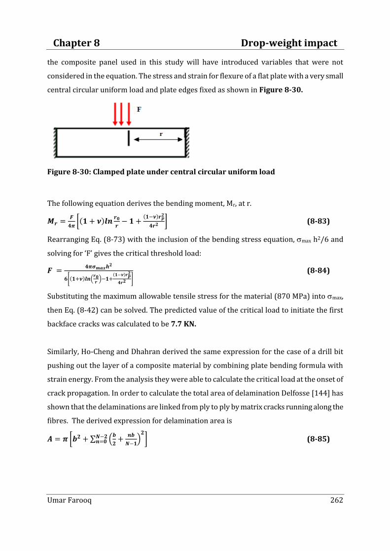
Chapter 8 Drop-weight impact
Umar Farooq 262
the composite panel used in this study will have introduced variables that were not
considered in the equation. The stress and strain for flexure of a flat plate with a very small
central circular uniform load and plate edges fixed as shown in Figure 8-30.
Figure 8-30: Clamped plate under central circular uniform load
The following equation derives the bending moment, Mr, at r.
𝑴𝒓 =𝑭
𝟒𝝅 𝟏 + 𝝂 𝒍𝒏
𝒓𝟎
𝒓− 𝟏 +
𝟏−𝝂 𝒓𝒑𝟐
𝟒𝒓𝟐 (8-83)
Rearranging Eq. (8-73) with the inclusion of the bending stress equation, max h2/6 and
solving for ‘F’ gives the critical threshold load:
𝑭 =𝟒𝝅𝝇𝒎𝒂𝒙𝒉𝟐
𝟔 𝟏+𝝂 𝒍𝒏 𝒓𝟎𝒓
−𝟏+ 𝟏−𝝂 𝒓𝒑
𝟐
𝟒𝒓𝟐
(8-84)
Substituting the maximum allowable tensile stress for the material (870 MPa) into max,
then Eq. (8-42) can be solved. The predicted value of the critical load to initiate the first
backface cracks was calculated to be 7.7 KN.
Similarly, Ho-Cheng and Dhahran derived the same expression for the case of a drill bit
pushing out the layer of a composite material by combining plate bending formula with
strain energy. From the analysis they were able to calculate the critical load at the onset of
crack propagation. In order to calculate the total area of delamination Delfosse [144] has
shown that the delaminations are linked from ply to ply by matrix cracks running along the
fibres. The derived expression for delamination area is
𝑨 = 𝝅 𝒃𝟐 + 𝒃
𝟐+
𝒏𝒃
𝑵−𝟏 𝟐
𝑵−𝟐𝒏=𝟎 (8-85)

Chapter 8 Drop-weight impact
Umar Farooq 263
8.9 Summary
The drop-weight flat and round nose low velocity impact tests on carbon fibre laminates
were performed. Post-impact visual inspections, Eddy-current, and C-scan tests were
carried out to approximate impact induced damage. Impact induced damage from flat and
round nose impactors were compared in the form of damage zones and data plots. Results
were validated against quasi-static test results, analytically determined parameters, and
data available from the literature and found within acceptable (±12%) deviations. Based on
comparison of the results, influence of flat and round impacts can be summarised as:
1) No visible damage was found for relatively low velocity impacts (up to 1.7 m/s)
from both types of impactor noses.
2) The study confirmed that relatively thin 8-Ply laminates were severally damaged by
flat nose impactor.
3) Damage inflicted by flat nose was global, spread over and internal compared to
round nose impact local damage.
4) The impact response of the laminates changes significantly under both the
impactors with increased thickness of laminates (16- and 24-Ply). The reason of this
behaviour is the flexural and contact stiffness which varies against impactor nose
profiles. The flexural and contact stiffness also vary according to thickness and
thereby causing the impact behaviour of a structure to change.
5) The reliably threshold load value correlates to delaminated/failed plies hence, no
further compression after impact testing is required. Moreover, reliably predicted
threshold values can be utilised in micro-macro mechanics formulations to
determine other selected parameters.
The use of a level of visible or non-visible damage may reduce the need for a
dynamic analysis and measurement of the residual strength irrespective of kinetic
energy or impact force. The work demonstrated that laboratory test data can be
used directly to predict other impact parameters concurrently via inter
relationships of the testing, theory, and numerical areas.

Chapter 8 Drop-weight impact
Umar Farooq 264
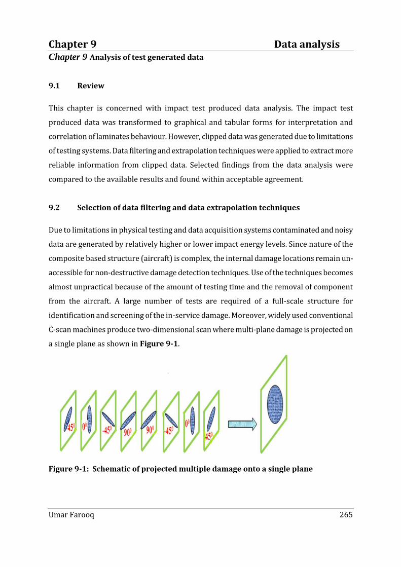
Chapter 9 Data analysis
Umar Farooq 265
Chapter 9 Analysis of test generated data
9.1 Review
This chapter is concerned with impact test produced data analysis. The impact test
produced data was transformed to graphical and tabular forms for interpretation and
correlation of laminates behaviour. However, clipped data was generated due to limitations
of testing systems. Data filtering and extrapolation techniques were applied to extract more
reliable information from clipped data. Selected findings from the data analysis were
compared to the available results and found within acceptable agreement.
9.2 Selection of data filtering and data extrapolation techniques
Due to limitations in physical testing and data acquisition systems contaminated and noisy
data are generated by relatively higher or lower impact energy levels. Since nature of the
composite based structure (aircraft) is complex, the internal damage locations remain un-
accessible for non-destructive damage detection techniques. Use of the techniques becomes
almost unpractical because of the amount of testing time and the removal of component
from the aircraft. A large number of tests are required of a full-scale structure for
identification and screening of the in-service damage. Moreover, widely used conventional
C-scan machines produce two-dimensional scan where multi-plane damage is projected on
a single plane as shown in Figure 9-1.
Figure 9-1: Schematic of projected multiple damage onto a single plane

Chapter 9 Data analysis
Umar Farooq 266
Another major issue of the scanning is the large amount of data to have sufficient resolution
to detect a small crack within a large area. Thus, inter-laminar damage often goes
undetected that could severely reduce compressive strength and is major concern to
aircraft industry. Since real structures are complex and impact events of the structures are
uncertain. The non-destructive damage detection methods could not gather and translate
meaningful data that could be used in design laboratories. Researchers have incorporated
data analysis techniques beside non-destructive testing techniques to complement the
damage diagnostics. Computational techniques are becoming powerful and easier to use.
Data processing, data filtering, and plotting facilities are assisting designers with invaluable
tools to extract enhanced information about the mechanisms involved in impact damage:
initiation, propagation and prediction. Data interpretation, analysis, and correlation could
create link between observed damage to applied load through processed plots. The
correlation simplifies and group damage into categories associated with failure modes
though plots as shown in Figure 9-2.
Figure 9-2: Schematic of possible damage modes [21].
The correlation among measured quantities could be efficiently enhanced for any possible
relation among known to unknown quantities. The same data analysis techniques were
selected to investigate the post-impact damage behaviour of impacted laminate. Impact
produced quantities were recorded for: displacement, velocity, energy and force history of

Chapter 9 Data analysis
Umar Farooq 267
the sets of 8-, 16-, and 24-Ply laminates subjected to round and flat nose impactors. An
outline the investigation is depicted in flowchart Figure 9-3. Impact produced data was
analysed using built-in, statistical, numerical and fast Fourier filters.
Figure 9-3: Flowchart depicting stages of present work.
The examinations of the experimental results were assisted with the use of digital filters.
The aim of the filtering was to remove the low frequency impact response of the plate so it
would not dominate the high frequency signals. The instrumented filtering is widely used
for evaluating the impact damage of composites. The development of photographic
techniques for observing the impact process and the recognition that the level of filtering of
the force-time signal can significantly affects the results. The ability to monitor force-time
signals the course of impact deformation offered considerable potential over tests that
merely articulated input energy to a specimen. The first effect is to remove the small
oscillations which are observed in the unbroken specimen, and essentially are oscillations
of the impactor. At a lower frequency the curve becomes distorted, shifting towards longer
times (larger deflections) and is reduced in height. It is clear that too much filtering
significantly distorts the signal and that the forces and energies registered are reduced,
even in this case where the curve is gently rounded. By taking a set of photographs, each at
a different time after the start of impact, it is possible to start to resolve the meaning of
Chapter 9 Data analysis
Umar Farooq 268
different peaks in the force-time curve. This material principally fails by the initiation and
growth of a variety of cracks. The material is also stiff and fails at a small stresses and hence
small deflections. Signals from the critical regions then give rise to incorrect quantitative
data analysis.
9.3 Data filtering based on built-in filters (data acquisition system)
9.3.1 8-Ply laminate impacted at different velocities
Drop-weight impact tests were conducted on 8-Ply laminate using flat nose impactor data
recorded from two impact tests at velocity 2.2 m/s was filtered and plotted in. Both the
curves show consistent behaviour and load drop at around 7 KN that indicates failure.
Built-in filtered data gathered from impact velocity: 2.41 and 3.12 m/s were plotted in
Figure 8-23. Comparison of the plot shows different level of curves for different impact
velocities. Load drops around 5.5 KN indicating failure and consistent behaviour are
obvious. This indicates that the data acquisition system and built-in filtered could genuinely
gather and filter data for this range of impact velocities and laminates.
9.3.2 8-Ply laminate impacted from different nose profiles
Drop-weight impact tests were conducted on 8-Ply laminate using flat and round nose
impactors. Data from two tests were recorded and filtered from impact at velocity 2.2 m/s
was plotted in Figure 7-10. The curve representing data plot from flat nose impactor
shows load drop around 7 KN while round nose curve shows load drop around 3.5 KN. The
plot clearly differentiates difference in damage associated with impactor nose profiles.
Similarly, data from two tests recorded and filtered from impact at velocity 2.4 m/s was
plotted in Figure 9-4. The curve representing data plot from flat nose impactor shows load
drop at around 8 KN while round nose curve shows load drop around 4 KN. The consistent
behaviour can be seen from the plots where load drops in all the cases indicate failure. This
indicates that the data gathered and filtered can be used to analyses impact behaviour of
laminate impacted from flat and round nose impactors for this range.

Chapter 9 Data analysis
Umar Farooq 269
Figure 9-4: Load-deflection response of 8-Ply laminates.
9.3.3 Energy history for 8-Ply laminate
The impact velocity for both the impactor nose shape is the same 2.2 m/s. It can be seen
from round nose shape curve Figure 9-5 that there is no elastic energy under the curve its
behaviour is almost stable. However, impact velocity level under flat nose curve has
changed considerably. The drop in impact energy from 12 J to 6 J can be attributed to the
50% energy absorbed by the impact from flat nose. This indicates that the gathered and
filtered can also predict energy levels particularly the absorbed energy.
Figure 9-5: Energy-history plot of 8-Ply laminate round and flat nose impactors

Chapter 9 Data analysis
Umar Farooq 270
9.3.4 Comparison of load, displacement, velocity, and deflection history
Graphic comparisons of the test generated and filtered data were correlated to the
fluctuations in applied load to interpret useful information about how material behaves
during the impact process. Selected plot of deflection curves under flat nose impact of 8-Ply
laminate at 2.2 m/s velocity trace in
Figure 9-6(a) were compared to plot in
Figure 9-6(b). The deflection curves show 8 KN load and significant drop in load curve
indicating ply failure at 1.5 ms from flat nose impactor.
Figure 9-6: a) Velocity, load and deflection histories; flat nose compared to b).
While the 4 KN load drop in load curve for round nose impactor at time 2.5 ms. The plot
shows that flat nose impactor create more damage than the round nose impactor when
laminates are relatively thin
Figure 9-7(a) and (b). This indicates that the data gathered and filtered from the type of
impact events can predict correlation and behaviour for other parameters.

Chapter 9 Data analysis
Umar Farooq 271
Figure 9-7: a) Velocity, load and deflection history; round nose against b).
9.3.5 Limitations of the built-in filters
To investigate influence from the flat and round nose impacts of 8-Ply laminates of 2.88 mm
thickness at velocity 1.7 m/s raw/random data was plotted for impact rebound in Figure
9-8(a). Plot shows unfiltered, jumbled peak and load values; useful information cannot be
extracted from data plots. Another plot of 8-Ply laminate was plotted in Figure 9-8(b). No
sudden/abrupt load drop fluctuation or load drop can be seen (a smooth bell shape curves)
from curves plotted for both the impactor noses. This indicates that using built-in filters
internal damage cannot be readily predicted for the impact velocity range up to velocity 1.7
m/s impacted from different impact nose.
Figure 9-8: Load deflection comparison of 8-Ply laminate at velocity 1.7 m/s.

Chapter 9 Data analysis
Umar Farooq 272
Drop-weight impact tests were carried out on 8-Ply laminates from flat and round nose
impactors at 1.6m/s velocity. To assess and investigate damage the test generated data was
recordedduring the impact process and column-chart was drawn. No significant difference
can be seen from the comparison in damage quantities created from flat and round nose
impactors as shown in Figure 9-9.
Figure 9-9: Load-deflection comparison of 8-Ply response at velocity 1.6 m/s
To confirm influence from the flat and round nose impacts comparisons were also carried
out against C-scanned images and Eddy-current surfaces. The C-scan images show
negligible damage on both the laminate surfaces as shown in Figure 7-9(a). Similarly,
surfaces drawn using from Eddy-current generated data show no difference in impact from
both the nose profiles Figure 7-9(b). Based on the comparisons supported by both the
non-destructive methods confirmed that built-in cannot readily differentiate damage from
flat and round nose impactors up to velocity 1.7 m/s. The consistent and coincident curves
and images look if data were generated from identical nose impactors. The limitations
could be attributed to: thin laminate, impacting machine, and data logging systems. Useful
information cannot be extracted from data plots due to narrow band of data points for
slope of clipped-data. Comparisons of data gathered and filtered by built-in system for 16-
Ply and 24-Ply laminates shown potion of clipped data hence results were not reported.

Chapter 9 Data analysis
Umar Farooq 273
9.4 Data filtering using statistical (moving average) methods
Moving average method is the widely used method being used for data filtering and data
extrapolation in science and engineering applications. The cases in which the time series is
fairly stable one can use smoothing methods to average out the irregular component of the
time series. Common moving average (smoothing) methods are: moving averages,
weighted moving averages, and centered moving average. Higher order methods can be
used to smooth large amount of oscillatory and for missing data. The moving averages
method consists of computing an average of the most recent data values for the series and
using this average to predict the value of the time series for the next period. Moving
averages are useful if one can assume item to be predicted stays fairly steady over time
designed to level out the large fluctuations. To predict the missing value a three-point
moving average method was utilised. The solution process is given in Table below.
Example 9-1: Three-point moving average method
The typical data values consisting of time interval [.2 .4 .6 .8 1. 1.2] as shown in column 1
and y-values [4 6 5 3 7 ?] are shown in column 2. The data has a contaminated (missing)
value at 1.2 ms in 7th row and column 2. It is desired to predict the missing value. Applying
the three-point moving average method as explained in Table 9-1 the predicted value
comes out ‘5’ in row 7and column 4.
Table 9-1: An example of three-point moving average method

Chapter 9 Data analysis
Umar Farooq 274
9.4.1 16-Ply laminate comparison of impact velocity and impactor nose
Drop-weight impact tests were conducted on 16-Ply laminate using flat and round nose
impactors. Data from two tests at velocity 3.12 m/s were recorded, filtered, and plotted in
Figure 9-10(a) & Figure 9-10(b). The elastic impact and rebound curve for round nose
shows consistent behaviour to some extent, the load drops around 11 KN that indicates
failure. However, filtered data gathered from flat nose impact shows inconsistent
behaviour. Instead of load drop it shows constant loading line like plastic behaviour.
Figure 9-10: Load-deflection plot of 16-Ply laminate; round and flat impacts.
To further investigate the behaviour another comparison was extended for slightly higher
impact velocity plot shown in Figure 9-11(a) & Figure 9-11(b). Comparison shows similar
behaviour. Comparisons of results indicate that the statistical filtered could not readily
predict behaviour of 16-Ply laminates subjected to flat nose impactors.
Figure 9-11: Load-deflection of 16-Ply laminate; round and flat nose impactors.

Chapter 9 Data analysis
Umar Farooq 275
9.4.2 16-Ply laminate energy history
The representative energy history plot of 16-Ply laminate impacted at 3.12 m/s and is
shown in Figure 9-12. Influence from the impactor nose can be assessed though
correlating energy phases to the damage mode shapes. Despite same velocity both the
impactor attain different impact energy levels. Contrary to 8-Ply laminate slightly increased
impact energy level due to round nose impact. Absorbed energy curve starts increasing
after 2 second in the case of impact from flat nose impactor. Both types of impacts have
generated vibrations and there phases of elastic energies. Impact from round nose depicts
smooth trends after one second of the impact time. Influence of the impact from flat nose
remains for seven seconds and it finishes after ten seconds. As the contact of the flat nose
remains for a longer time period, it therefore, generates more internal damage than the
round type of impactor. The curve representing round nose shape shows peak energy level
at 27 J while peak load for flat nose impactor is indicated at 24 J. The absorbed energy
curve under flat nose impactor shows approximate absorbed up to 50% of the impact
energy. The impact energy curve of the round nose impact drops to 20 J which could be
approximated to 35% absorbed energy. Impact energy-time curves remain constant. At
these curves, the highest tip of the curve shows maximum impact energy and the end of the
curve shows the absorbed energy.
Figure 9-12: Energy-histories of 16-Ply laminate at velocity 3.12 m/s
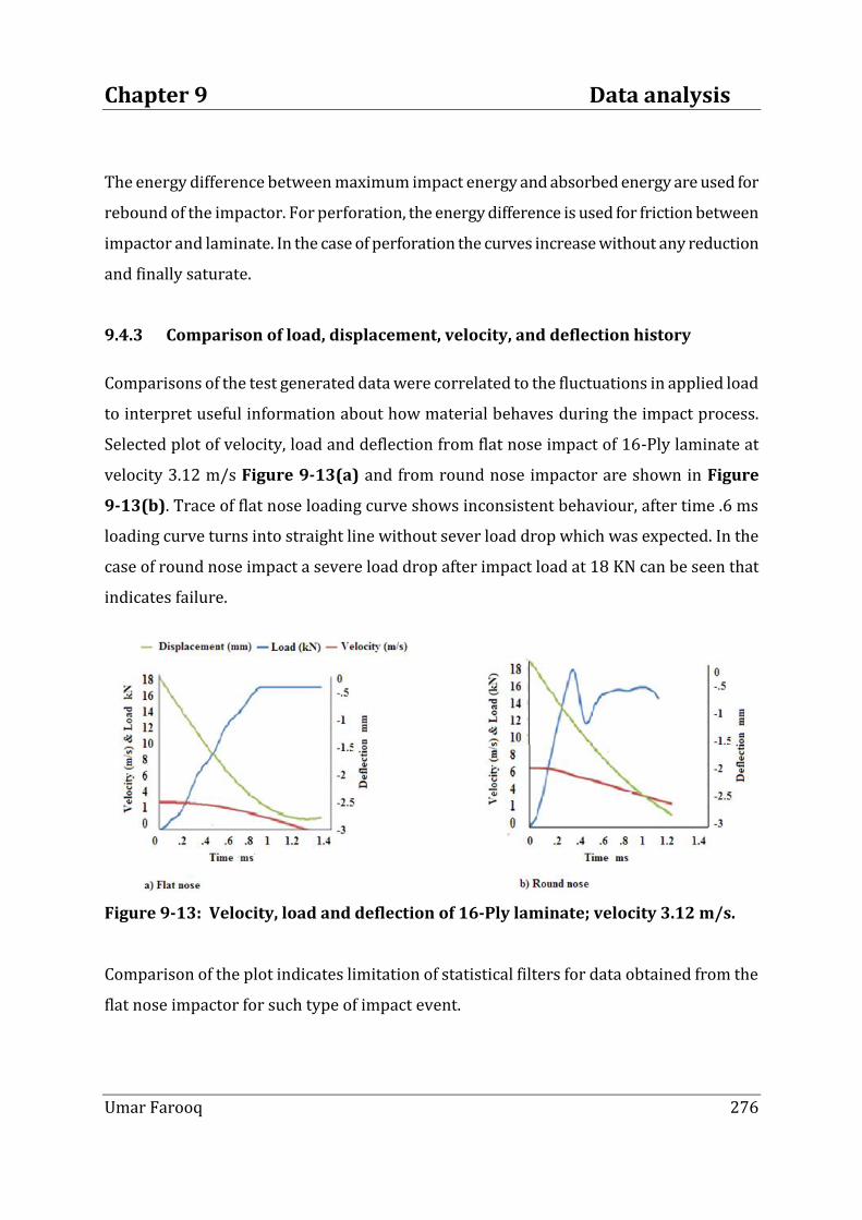
Chapter 9 Data analysis
Umar Farooq 276
The energy difference between maximum impact energy and absorbed energy are used for
rebound of the impactor. For perforation, the energy difference is used for friction between
impactor and laminate. In the case of perforation the curves increase without any reduction
and finally saturate.
9.4.3 Comparison of load, displacement, velocity, and deflection history
Comparisons of the test generated data were correlated to the fluctuations in applied load
to interpret useful information about how material behaves during the impact process.
Selected plot of velocity, load and deflection from flat nose impact of 16-Ply laminate at
velocity 3.12 m/s Figure 9-13(a) and from round nose impactor are shown in Figure
9-13(b). Trace of flat nose loading curve shows inconsistent behaviour, after time .6 ms
loading curve turns into straight line without sever load drop which was expected. In the
case of round nose impact a severe load drop after impact load at 18 KN can be seen that
indicates failure.
Figure 9-13: Velocity, load and deflection of 16-Ply laminate; velocity 3.12 m/s.
Comparison of the plot indicates limitation of statistical filters for data obtained from the
flat nose impactor for such type of impact event.

Chapter 9 Data analysis
Umar Farooq 277
9.4.4 Load and energy for different lay-ups
Another comparison was made to explore the inconsistency in impact behaviour of 16-Ply
laminate in Figure 9-14(a) and 24-Ply laminates is made in Figure 9-14(b). Plot shows
almost the same energy levels but significant difference in loading curves. This supports the
arguments that data obtained related to the applied load for such impacts cannot be readily
predicted by using moving average filters.
Figure 9-14: Load, energy history of 16-Ply and 24-Ply laminate responses.
9.4.5 Higher order moving average methods
To further investigate the inconsistencies and efficiency of filter’s type a high order moving
order repeated data filtering were carried out to predict threshold load. It can be seen from
the plots that the higher order filters make predictions less sensitive to changes as shown
in Figure 9-15(a) and Figure 9-15(b). That confirmed that the flat nose impact behaviour
of laminate through fluctuations in applied load for such impacts cannot be readily
predicted by using moving average filters.

Chapter 9 Data analysis
Umar Farooq 278
Figure 9-15: Load, energy history of 16-Ply response with high order filter.
9.4.6 Limitations of the statistical (moving average) filters
The moving average process lags behind increasing data and leads the decreasing data
values. The methods require sufficient historical data values. The method does not predict
trends well to improve clipped and data band consisting of straight lines. Higher order
filters make predictions less sensitive to changes.
9.5 Data filtering using numerical techniques
More reliable and robust methods are based on numerical analysis techniques.
Extrapolation of numerical values consists of using the curve fitting techniques to estimate
data quantities and then extend predictions based upon the estimated data. Curve-fitting of
a line calculates a future value by utilising the existing x- and y-values. The new value is
predicted by using linear regression. The equation for fitting the data to a linear line is
𝒚 = 𝒂 + 𝒃𝒙 (9-1)
Where: 𝒂 = 𝒚 − 𝒃𝒙 ; 𝒃 = 𝒙−𝒙 𝒚−𝒚
𝒙−𝒙 𝟐 and 𝒙 =
𝒙
𝒏; 𝒚 =
𝒚
𝒏.
Based on the available dada the best-fit could more reliably a future value.
Once estimate of the future value is obtained further extrapolated can be easily estimated
by applying Huen’s predictor-corrector method given below. The method uses slope at the
beginning of an interval

Chapter 9 Data analysis
Umar Farooq 279
𝒅𝒚
𝒅𝒙=
𝒚𝟐−𝒚𝟏
𝒙𝟐−𝒙𝟏= 𝒚𝒊 = 𝒇(𝒙𝒊, 𝒚𝒊) (9-2)
is used to extrapolate linearly to 𝑦𝑖+1:
𝒚𝒊+𝟏𝟎 = 𝒚𝒊 + 𝒇 𝒙𝒊, 𝒚𝒊 𝒉 (9-3)
This is also called the predictor equation. It produces an estimate of 𝑦𝑖+1:that allows the
calculation of an estimated slope at the end of the interval:
𝒚𝒊+𝟏′ = 𝒚𝒊 + 𝒇 𝒙𝒊 + 𝟏, 𝒚𝒊+𝟏
𝟎 𝒉 (9-4)
Eqns. (9-2) and (9-4) can be combined to obtain an average slope
𝒚 = 𝒚𝒊 +𝒚𝒊+𝟏
′
𝟐=
𝒇 𝒙𝒊,𝒚𝒊 +𝒇 𝒙𝐢+𝟏,𝒚𝒊+𝟏𝟎
𝟐𝒉 (9-5)
The average slope is then used to extrapolate linearly from 𝑦𝑖 to 𝑦𝑖+1 using Euler’s method
𝒚𝒊+𝟏 = 𝒚𝒊 +𝒇 𝒙𝒊,𝒚𝒊 +𝒇 𝒙𝒊+𝟏,𝒚𝒊+𝟏
𝟎
𝟐𝒉 (9-6)
This is the correction method.
Utilising previous values and the predicted best-fit future value the predictor-corrector
techniques could reliably predict a reasonable band of future quantities. Graphical
representation of the formulation is shown in Figure 9-16.
Figure 9-16: Numerical filter and extrapolation relations.

Chapter 9 Data analysis
Umar Farooq 280
However, the method cannot be applied to filter and extrapolate data herein as the method
is based on average values of slopes which are zeros for straight lines. Other widely used
algorithms are numerical integrations that could more reliably lead to a band of future
quantities. One such method is the modified Simpson’s rule regarded as inherent filter.
Simpson’s rule is a method of finding areas under a curve using an approximate integration
method. The next part of Simpson’s rule is regression. This results in an equation for
velocity that can be used to calculate other values such as displacements by similar
integration. Other value that can be obtained from this is the force if mass of free falling
weight and the acceleration are known. The modified Simpson’s rule Eq. (6-63) of Chapter
7 was selected. As interval [a, b] is split up in n sub-intervals, with n an even number where
equidistant x values are x0, x1, ..., xn, the step width being ℎ = 𝑏 − 𝑎
𝑛 . The composite
Simpson's rule given by the 2nd order polynomials (parabolas) for approximating the curve
to be integrated can be written as:
𝒇 𝒙 𝒅𝒕 ≈𝒉
𝟑 𝒇 𝒂 + 𝒇(𝒃) + 𝟐 𝒇 𝒙𝟐𝒌 + 𝟒 𝒇(𝒙𝟐𝒌−𝟏)
𝒏𝟐
𝒌=𝟏
𝒏𝟐 −𝟏
𝒌=𝟏
𝒃
𝒂 (9-7)
The area needs to be divided into equally spaced intervals of uniform width. The algorithm
uses Eqn. (9-7) to compute area:
Area = 𝒉
𝟑 𝑨 + 𝟐𝑩 + 𝟒𝑪 (9-8)
Where: A is sum of first and last ordinates; B is the sum of remaining ordinates, and
C is the sum of even ordinates and h is width of a strip. Application of the algorithm is illustrated in
Table 9-2.
9.5.1 16-Ply and 24-Ply laminate prediction of energy
The energy absorbed by the laminate during impact can be quantified by evaluating the
area under the curve. Area under the load-deflection curve was numerically integrated
using Simpson’s modified rulee Eq. (9-7) to estimate impact energy of 16- and 24-Ply
laminates. Code is shown in Table 9-2 below.

Chapter 9 Data analysis
Umar Farooq 281
Table 9-2: Code for modified Simpson rule
Input: a, b, and n;h = (b-a)/n; x = zeros(1,n+1);
x(1) = a; x(n+1) = b;p = 0;q = 0;% the x-vector
for i = 2:n
x(i) = a + (i-1)*h; end % multiples by 4
for i = 2:((n+1)/2)
p = p + (f(x(2*i -2)));end % multiples by 2
for i = 2:((n-1)/2)
q = q + (f(x(2*i -1))); end % Calculate final output
x = (h/3)*(f(a) + 2*q + 4*p + f(b));
function x = compsimp (a,b,n,f)% Function the Simpson's rule
h = (b-a)/n; x = zeros(1,n+1); x(1) = a; x(n+1) = b;p = 0;q = 0; % Define the x-vector
for i = 2:n; x(i) = a + (i-1)*h; end % multiples by 4
for i = 2:((n+1)/2); p = p + (f(x(2*i -2)));end % multiples by 2
for i = 2:((n-1)/2)
q = q + (f(x(2*i -1))); end % Calculate final output
x = (h/3)*(f(a) + 2*q + 4*p + f(b)); % Define the x-vector
for i = 2:n; x(i) = a + (i-1)*h;end % multiples by 4
for i = 2:((n+1)/2)
p = p + (f(x(2*i -2)));end % the terms multiples by 2
for i = 2:((n-1)/2)
q = q + (f(x(2*i -1))); end % Calculate final output
x = (h/3)*(f(a) + 2*q + 4*p + f(b));End
The numerical integration of the areas under the curve produce energy estimates 21 J for
unfiltered values and 24 J from the flat nose filtered values using the Eq. (9-8) for 16-Ply
laminate shown in Table 9-3.

Chapter 9 Data analysis
Umar Farooq 282
Table 9-3: numerical integration to estimate area under the curve
Deflection
mm
Round
Impactor
Flat Impactor Simpson’s
multiplier
Area under the curve J
Load KN Load
KN
Filtered
Load (k N)
Unfiltered Filtered
0.25 0 .6 .6 1 0.6 0.6
0.5 2 1.6 1.6 4 0.64 0.64
0.75 3.5 2.1 2.1 2 0.42 0.42
1 6 5.6 5.6 4 2.24 2.24
1.25 7 7.6 7.6 2 15.2 15.2
1.5 10 8.4 8.4 4 33.6 33.6
1.75 11.5 10.2 10.2 2 204 204
2 8.9 13 13 4 52.0 52.0
2.25 9.5 14 14 2 28.0 28.0
2.5 9.2 16 16 4 64.0 64.0
2.75 9.3 16 20.1 2 32.0 40.
3 9.6 16 18.1 1 16.0 18.08
Energy J 21.23 24.1
Similarly, areas under the curve produce energy estimates 30 J for unfiltered values and 36
J from the flat nose filtered values for 24-Ply laminate. The results indicate that numerical
integration could predict acceptable estimate of energy values from the impact produced
data of such types Table 9-4.

Chapter 9 Data analysis
Umar Farooq 283
Table 9-4: numerical integration to estimate area under the curve
Numerically predicted energy values compared against experimentally obtained energy
levels and values calculated from the energy formulation as shown Table 9-5. Comparison
of the values agreed well with (±5%) deviations.
Table 9-5: Comparison of energy values
Laminate
Energy J
Experimental Calculated Estimated (graphical)
( E = ½ mV2) Un-filtered Filtered
16 24 25.66 23.23 26
24 34 35. 30.41 36.
Deflection
mm
Round nose
Flat nose
Simpson
Multiplier
Area under the curve J
Load KN Load
KN
Filtered
Load KN
Un-filtered Filtered
0.25 0.5 1.8 1.8 1 1.8 1.8
0.5 0.5 3.7 3.7 4 14.8 14.8
0.75 0.2 8 8 2 16.0 16.0
1 0.8 12 12 4 48.0 48.0
1.25 2 14.2 14.2 2 28.4 28.4
1.5 4 16 16 4 64.0 64.0
1.75 6 16 18.5 2 32.0 36.98
2 8 16 20.2 4 64.0 80.88
2.25 12 16 21.7 2 32.0 43.37
2.5 12 16 22.81 4 64.0 91.27
30.41 36.45

Chapter 9 Data analysis
Umar Farooq 284
9.5.2 Comparison of load, displacement, velocity, and deflection history
Comparisons of the test generated data for 24-Ply laminate impacted at 3.74 m/s were
plotted in Figure 9-17(a). Curves relating to flat nose impact for velocity and deflection
parameter show consistent behaviour. However, load history shows an inconsistent
behaviour and load drop after as if plastic deformation which was not expected. The
comparison of round nose data plot Figure 9-17(b) also shows similar unexpected pattern
and trends. The comparison indicates that data generated from such impacts of 24-Ply
laminates could not be readily filtered using numerical techniques and analysed for impact
load fluctuations to predict threshold load.
Figure 9-17: Load, velocity and deflection of 24-Ply laminate at velocity 3.74 m/s.
9.5.3 16-Ply and 24-Ply laminates versus flat and round nose impactors
Drop-weight impact tests were conducted on 16-Ply and 24-Ply laminates using flat and
round nose impactors at velocity 3.12 m/s. Data from two flat nose impact tests was
recorded, filtered and plotted in Figure 8-16(a). The elastic impact and rebound curves for
flat nose impactor shows inconsistent behaviour to some extent and load drops after sort of
plastic behaviour around 17 KN. This indicates limitations of the filter that could be

Chapter 9 Data analysis
Umar Farooq 285
attributed to the laminate thicknesses that’s why filtered data gathered from flat nose
impact shows inconsistent behaviour. Similar behaviour can be seen for 24-Ply laminated
impacted by round nose impactor shown in Figure 8-16(b). However, consistent
behaviour can be seen for round nose impact on 16-Ply laminate. This indicates that
numerical filter can predict threshold load for laminate impacted by round nose impactors.
9.5.4 Limitations of the filters based on numerical techniques
The process is complicated and involves combination of numerical methods to reach a
reliable future value. Parts of data consisting of little interference or noise and parts of
significant peaks could be lost due to heavy filtering. Removal of force and energy from
critical regions will give rise to incorrect quantitative data during further analysis.
Numerical integration requires reliable initial value is required to predict next estimates.
Moreover, numerical methods based filters cannot readily improve data-bands consisting
of straight lines.
9.6 Data filtering and extrapolation using Fast Fourier algorithms
9.6.1 Fast Fourier algorithms as filters
Common filtering objectives are to improve the quality of a signal e.g., reduce noise, or to
extract information from signals. Impact testing can be used to gain information on the
material and structure of a particular laminate showing in the form of data or signals. Once
data has been collected in the raw format, it can be analysed using various techniques. One
method is the Fourier analysis. Fourier analysis is a way of mapping curves and finding
areas under the curve. The ability of finding area under a curve can be used to find other
characteristics such as velocities, displacements and acceleration. Once these
characteristics have been found other mathematical process can be used to find more
values that can be useful such as force. However sometimes when the signal is being

Chapter 9 Data analysis
Umar Farooq 286
produced a phenomenon of noise is sometimes found distorting the acquired signal. This
can seriously alter values within the signal and subsequently cause the analysis to form
error. In order to get a signal correct, the data must go through a filter. However the filters
depend on filtering certain aspects of the signal such as frequency, the signal needs to be
transferred by a process like Fast Fourier Transformation in order for filtering to take
place. Any periodic waveform can be represented as the sum of an infinite number of
sinusoidal and co-sinusoidal terms, together with constant terms this representation is
known as the Fourier series for example varying voltage versus time waveform. The Fast
Fourier Transformation (FFT) can be realised as a program to turn a signal from the time
domain to the frequency domain, or from the frequency domain into the time domain. The
FFT provides spectral components of signals between zero and one half the sampling
frequencies that require a less computational time and effort than that of Discrete Fourier
Transforms. It works as a system for passing the spectral contents of an input signal in a
certain specified band of frequencies, the filter transfer functions from a window in the
frequency domain through which a portion of the input spectrum is allowed to pass. There
are various types of filters which include low pass, high pass, band pass and band stop. A
filter is essentially a system or network that selectively changes the wave shape, amplitude
and frequency characteristics of a signal in a desired manner. Once constants are found the
equations can be used to map the Fourier curve of the data. The FFT allows converting data
or signal from the time domain to the frequency domain. This allows manipulation of data
using filters to analysis and extract information. The use of filters allows noise to be
separated from the original data so as to build a clear image of true data by separating
different types of information from the data. Writing the formula:
𝑮 𝒊𝒘 = 𝒈 𝒕 𝒆−𝒊𝒘𝒏𝒕 (9-9)
and integrating by parts produces
𝑮 𝒊𝒘 = 𝒆−𝒊𝒘𝒏𝒕 𝒈 𝒕 𝟐
𝟐 +
𝟏
−𝒊𝒘𝒏 + 𝒄 (9-10)
Assuming c= -1 and 𝑒−𝑖𝑤𝑛𝑡 ≈ 1 gives:
𝑮 𝒊𝒘 = 𝒈 𝒕 𝟐
𝟐−𝒊𝒘𝒏 (9-11)
Multiplying the top and bottom by 2 − 𝑖𝑤𝑛 and re-factorising we can get:
𝑮 𝒊𝒘 = 𝒈 𝒕 𝟐
𝟐−𝒘𝒏 (9-12)

Chapter 9 Data analysis
Umar Farooq 287
This is the transfer function from the time domain to the frequency domain. To convert
back to the time domain we use this function:
𝒈 𝒕 = 𝟏
𝟐𝝅 𝑮 𝒊𝒘 𝒆−𝒊𝒘𝒏𝒕 (9-13)
Once the input and output signal have been converted from time domain to the frequency
domain further manipulation is required to put the data into a suitable format so that
filtering can take place. Conventional filterer were applied to smooth highly oscillatory
data however plots in current case consist of portions Figure 9-17 of straight lines that
have no oscillatory components. Fourier methods transform data into circular domain and
transform non-periodic data into period forms. Hence, Fourier types of filters were selected
for this work. Filters alter the frequency response (both magnitude and phase) of a signal
Figure 9-18.
Figure 9-18: Schematics of Fourier filter process.
In the frequency domain the filtering process is a simple case of multiplication:
𝒀 𝒘 = 𝑿 𝒘 . 𝑯 𝒘 (9-14)
Where: Y() is the frequency content of the output (magnitude and phase)
X() is the frequency content of the input (magnitude and phase)
H() is the frequency response of the filter (magnitude and phase)
In the time domain the process of filtering is a convolution:
𝒚 𝒕 = 𝒙 𝒕 ⨂𝒉 𝒕 (9-15)
where y(t) is the output signal (as a function of time)
x(t) is the input signal (as a function of time)
h(t) is the impulse response of the filter

Chapter 9 Data analysis
Umar Farooq 288
and denotes convolution (explained in a moment)
h(t) is called the impulse response because it is the response (i.e., output) of the filter when
the input is a perfect impulse (i.e., a delta function). That is,
𝒉 𝒕 = 𝜹 𝒕 ⨂𝒉 𝒕 (9-16)
Equations (9) and (10) are related by the Fourier Transform as:
𝒀 𝒘 = 𝑭 𝒚 𝒕
𝑿 𝒘 = 𝑭 𝒙 𝒕
𝑯 𝒘 = 𝑭 𝒉 𝒕 (9-17)
Similarly, the inverse Fourier Transform gets us from the frequency to the time domain:
𝒚 𝒕 = 𝑭−𝟏 𝒀 𝒘
𝒙 𝒕 = 𝑭−𝟏 𝑿 𝒘
𝒉 𝒕 = 𝑭−𝟏 𝑯 𝒘 (9-18)
The process of filtering in the time domain is called convolution. Equation (9-18) above is
for continuous (analogue) signals and filters. The equivalent for discrete (digital) systems is
𝒚𝒏 = 𝒙𝒌⨂𝒉𝒌 (9-19)
Where: yn is the output signal (as a function of time), xk is the input signal (as a function of
time), hk is the impulse response of the filter and denotes convolution. Discrete
convolution is performed like this:
𝐲𝐧 = 𝐡𝐤𝐱𝐧−𝐤𝐍−𝟏𝐤=𝟎 (9-20)
where N is the total number of samples in x or h (whichever is the greater). Algorithm is
very efficient for computing no loss of data quality. Interpolating polynomial solves root of
unity. Symmetry and periodicity can be applied to split data into odd and even at every

Chapter 9 Data analysis
Umar Farooq 289
successive stage as shown below. Applying FFT procedure to determine Fourier
coefficients from complex constants ck for 16-data points xj yj 0
15.
Defining
𝐅 𝐱 =𝟏
𝟖 𝐜𝐤
𝟕𝐤=𝟎 𝐞𝐢𝐤𝐱 where 𝐜𝐤 = 𝐲𝐣
𝟕𝐤=𝟎 𝐞𝐢𝐣𝐱 (9-21)
So 1
8cke−ikx = ak + ibk for k = 0, 1, 2, … , 2m − 1 and 2m =16.
using divide and conquer algorithm
𝐜𝐤 + 𝐜𝐤+𝐦 = 𝐲𝐣𝟐𝐦−𝟏𝐣=𝟎 𝐞𝐢𝐣 𝛑
𝐤
𝐦 + 𝐲𝐣
𝟐𝐦−𝟏𝐣=𝟎 𝐞𝐢𝐣𝛑
𝐦+𝐤
𝐦
= 𝐲𝐣𝟐𝐦−𝟏𝐣=𝟎 𝐞𝐢𝐣𝛑 𝐤 𝐦 𝟏 + 𝐞𝐢𝐣𝛑 𝐟𝐨𝐫 𝐤 = 𝟎, 𝟏, 𝟐, … , 𝐦 − 𝟏 (9-22)
Where:
𝟏 + 𝐞𝐢𝐣𝛑 = 𝟐 𝐢𝐟 𝐣 𝐢𝐬 𝐞𝐯𝐞𝐧𝟎 𝐢𝐟 𝐣 𝐢𝐬 𝐨𝐝𝐝
(9-23)
This way root of unity gives another root of unity and a polynomial of N coefficients splits
into two polynomials of (N/2) coefficients. The splitting process into even and odd
alternatives is illustrated in example given below Table 9-6.
Table 9-6: Time domain decomposition of 16 point data through 4 stages
Similarly, roots of unity (w) and periodic symmetry is shown in Table 9-7 such properties
facilitate to computer root once and split the roots into odd and even. The process
considerably reduces computing time.

Chapter 9 Data analysis
Umar Farooq 290
Table 9-7: Roots of unity and periodic symmetry
9.6.2 Energy history for 24-Ply laminate
The representative history plots of 24-Ply laminate impacted at velocity 3.74 m/s is shown
in Figure 9-19 . Looking at the plot, the influence in respect of creating damage from the
impactor nose can be assessed. It is obvious that despite the same velocity both the
impactor attain slightly different impact energy levels. Increases impact energy, absorbed
(two phases), elastic energy zones depict the difference. The energy absorbed by the
laminate during impact can be quantified by evaluating the area under the curve. The
impact energy converted to elastic vibrations has also been reversed for different nose
profiles. This can be attributed to the thickness of the laminates. As plot representing
impact energy history of the laminate impacted from round nose shows exceeding in
elastic/vibration energy phase. The laminate in such case (impacted by round nose)
absorbs more energy through converting of the impact energy to elastic vibrations. Thus,
the laminate impacted by round nose generates high elastic energy that results in more
failure modes and mechanisms. Moreover, a small change (kink) in the curves rate can also

Chapter 9 Data analysis
Umar Farooq 291
be seen in the curve representing impact from the flat nose at around 14 J. This small
change can be attributed to the flexure deformation of the laminate. Impact, elastic and
absorbed energy levels have been depicted in the plot without using advanced filters.
Figure 9-19: Energy history of 24-Ply laminate impacted at velocity 3.74 m/s.
9.6.3 16-Ply and 24-Ply laminates versus flat and round nose impactors
Drop-weight tests were performed on 16-Ply laminates impacted by flat and round nose
impactors at impact velocity 3.74 m/s. Data filtered and recorded by built-in data
acquisition system were plotted. Observation of the plot in Figure 9-20 shows inconsistent
tendencies. Straight line after peak load (16 KN) when load drop was expected indicates a
constant resistance of the laminate to the applied load. This could be due to laminate
thickness. Generally, thickness factor increases proportional flexural rigidity that causes
dissipation of impactor energy into absorbed energy and frictional noise between laminate
and impactor.

Chapter 9 Data analysis
Umar Farooq 292
Figure 9-20: Load-deflection of 16-Ply at velocity 3.74 m/s
Another drop-weight test was performed on 24-Ply laminates impacted by flat and round
nose impactors at impact velocity 3.74 m/s was selected. Data filtered and recorded by
built-in data acquisition system were plotted. More inconsistent behaviour can be seen
from the plot in Figure 9-21. Hence advanced filtered are required.
Figure 9-21: Load-deflection of 24-Ply laminate at velocity 3.74 m/s

Chapter 9 Data analysis
Umar Farooq 293
9.6.4 Comparison of load, displacement, velocity, and deflection history
Comparisons of the test generated data for 24-Ply laminate impacted by flat and round
nose impactors at velocity 3.76 m/s are plotted in Figure 9-22(a) & Figure 9-22(b).
Similar inconsistent behaviour can be seen.
Figure 9-22: Velocity, load and deflection of 24-Ply laminate; a) and b) round
Another impact test at velocity 4.2 m/s in Figure 9-23(a) & Figure 9-23(b) was selected.
Curves relating to flat nose impact for velocity and deflection parameter show consistent
behaviour. However, load history shows an inconsistent behaviour and no load drop. The
comparison of round nose data plot also show similar pattern and trends. Based on the
results comparison it can be argued that data generated from such impact events cannot be
readily filtered using conventional data filtering techniques.
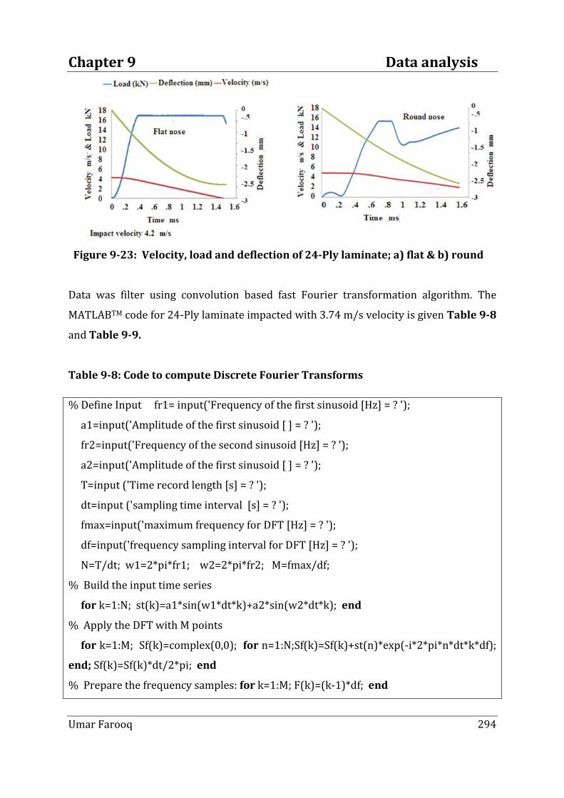
Chapter 9 Data analysis
Umar Farooq 294
Figure 9-23: Velocity, load and deflection of 24-Ply laminate; a) flat & b) round
Data was filter using convolution based fast Fourier transformation algorithm. The
MATLABTM code for 24-Ply laminate impacted with 3.74 m/s velocity is given Table 9-8
and Table 9-9.
Table 9-8: Code to compute Discrete Fourier Transforms
% Define Input fr1= input('Frequency of the first sinusoid [Hz] = ? ');
a1=input('Amplitude of the first sinusoid [ ] = ? ');
fr2=input('Frequency of the second sinusoid [Hz] = ? ');
a2=input('Amplitude of the first sinusoid [ ] = ? ');
T=input ('Time record length [s] = ? ');
dt=input ('sampling time interval [s] = ? ');
fmax=input('maximum frequency for DFT [Hz] = ? ');
df=input('frequency sampling interval for DFT [Hz] = ? ');
N=T/dt; w1=2*pi*fr1; w2=2*pi*fr2; M=fmax/df;
% Build the input time series
for k=1:N; st(k)=a1*sin(w1*dt*k)+a2*sin(w2*dt*k); end
% Apply the DFT with M points
for k=1:M; Sf(k)=complex(0,0); for n=1:N;Sf(k)=Sf(k)+st(n)*exp(-i*2*pi*n*dt*k*df);
end; Sf(k)=Sf(k)*dt/2*pi; end
% Prepare the frequency samples: for k=1:M; F(k)=(k-1)*df; end

Chapter 9 Data analysis
Umar Farooq 295
Table 9-9: Code to compute fast Fourier Transforms
% Get the input parameters
N=input ('N = ? ');
fr=input('Modulation frequency [Hz] = ? ');
dt=input ('time step, dt [s] = ? ');
w=2*pi*fr;
% Build the input time series
for k=1:N
X(k)=sin(w*dt*k)*exp(-(dt*N/(10*dt*k))^2);
end
% Apply the FFT
X2=fft(X,N);
X2=fftshift(X2); % swaps the left and right halves
X2=abs(X2);
% Prepare the frequency samples
fmax=1/dt; df=1/(N*dt);
for k=1:N
F(k)=-fmax/2+(k-1)*df;
end
% Plot the output
plot(F,X2); title('The FFT of a Time Signal')
xlabel('Frequency [Hz]'); ylabel('Amplitude')
%------------------------------- End of FFT.m –
x = [1 0.8 0.6 0.4 0.2]; % define input signal x_k
h = [1 1 1 1]; % define filter h_k
y = conv(h,x); % convolve x and h to form y
Extrapolated value can be obtained from magnitude of the FFT
It can be seen that from comparison of the flat nose filtered and un-filtered curves that peak
load quantity was raised from 18 KN to 21 KN approximately and for round nose impact

Chapter 9 Data analysis
Umar Farooq 296
load was raised from 15 KN to 18 KN. Moreover, a load drop indicating failure at peak
(threshold) load can be seen in Figure 9-24(a) and (b) under both the nose profiles.
Figure 9-24: Load-deflection plot of 24-Ply laminate filtered using Fast Fourier
The same filtering process was applied to the 24-Ply laminate impacted at velocity 4.2 m/s
plot is shown in Figure 9-25(a) and (b). It can be seen that the load from flat nose impact
increased from19 KN to 24 KN and for round nose impact load was increased from 15 KN
to 22 KN. Moreover, load drops in both the cases occurred that indicated peak loads as the
threshold loads. The comparisons of the results confirmed that the threshold load can be
predicted from such type of impact events using FFT based filters.
Figure 9-25: Load-deflection plot of 24-Ply laminate filtered using Fast Fourier

Chapter 9 Data analysis
Umar Farooq 297
9.6.5 Validation of the results obtained using Fast Fourier filters
A simple code based on mean value algorithm was developed as shown in Table 9-10.
Table 9-10: Code for extrapolation
Data filtering code
function y1_Callback(hObject, eventdata, handles)
y1 = str2num(get(handles.y1, 'String'));
function y2_Callback(hObject, eventdata, handles)
y2 = str2num(get(handles.y2, 'String'));
function ExtraP_Callback(hObject, eventdata, handles)
y1=str2num(get(handles.y1, 'String')); y2= str2num(get(handles.y2, 'String'));
y3=2*(y2)-y1; y3=num2str(y3); set(handles.value, 'String',y3);
9.6.5.1 Validation against available data
Using the code contaminated (missing) values were extrapolated for flat and round nose
impacts on 16-Ply laminate at velocity 3 m/s shown in Figure 9-26. The round nose impact
produced load drop at 10 KN when compared to the available value 8.9 KN in validates the
results. The predicted threshold load values were also compared to the analytically

Chapter 9 Data analysis
Umar Farooq 298
determined values from Example 2 of Eq. (8-33) and Eq. (8-74) and found within
acceptable range.
16-Ply laminate velocity 3 m/s
Figure 9-26: Load-deflection threshold load 10 KN validates 8.9 KN.
9.6.5.2 Validation of the results against statistical filter
Another plot was drawn using the code contaminated (missing) values were extrapolated
for flat and round nose impacts on 24-Ply laminate at velocity 3 m/s shown in Figure 9-27.
The un-filtered curve shows values filtered from statistical method but they remained as if
unfiltered. The plot shows that filtered values have increased to 24 KN from unfiltered
value 17 KN. The plotted data was compared to FFT produced results and found in
acceptable range. The results support validation of the data obtained using Fast Fourier
based filters for 24-Ply laminate velocity 4.2 m/s.
Load
KN

Chapter 9 Data analysis
Umar Farooq 299
Figure 9-27: Load-deflection plot validates predicted load 24 KN against 23 KN in
9.6.5.3 Validation of the results against mean value filter
To further explore the validation data generated from 16-Ply laminate impacted by flat and
round nose impactor at velocity 3.74 m/s was filtered and extrapolated using mean value
filter code in. Filtered curve shows Figure 9-28(a) and (b) that peak load quantity was
raised from 15 KN to 18 KN approximately. Moreover, a load drop indicating failure at peak
(threshold) load can be seen. The fat Fourier filtering process was applied to the data and it
can be seen that the load increased from 16 KN to 20 KN. Moreover, load drops in both the
cases occurred that indicated peak loads as the threshold loads.
Figure 9-28: Load-deflection comparison to predict threshold loads
The same raw data obtained from 16-Ply and 24-Ply laminates impacts at 3.74 m/s was
filtered using Fast Fourier algorithm (convolution based) in and. Filtered data was plotted
in Figure 9-29(a) and (b). Comparisons of the results confirm that threshold load values
are in acceptable range (±10%) deviations. Moreover, threshold load value 10 KN predicted
for round nose impactor agrees well to 8.9 KN threshold value reported in [1].

Chapter 9 Data analysis
Umar Farooq 300
Figure 9-29: Load-deflection comparison to predict threshold loads
Consistent results and acceptable agreement in comparisons to the available data in
literature confirmed and validate the results obtained using Fast Fourier filters.
9.7 Summary
Data generated from low velocity drop-weight flat and round nose impact of carbon fibre
laminates were filtered to predict impact response of the laminates. The fluctuations and
variations in applied load for impact duration were correlated to damage zones. Due to
limitations of the testing systems clipped data was generated. Advanced filtering
techniques were applied to extract information from clipped data. Based on the results
following conclusions can be extracted:
The built-in filters were used to de-noise data produced from impact of 8-Ply laminate and
predict threshold load. Statistical and numerical filters were used to filter impact induced
data for 16-Ply laminate to predict energy levels. However, due to limitations of built-in,
statistical, and numerical filters advanced filters based on Fast Fourier Transformation was
selected. The Fast Fourier Transformation combined with Convolution algorithm was used
to filter and extrapolate the clipped data that predicted threshold load. Comparison of the
FFT algorithms results were validated against mean-value filtered results. The results

Chapter 9 Data analysis
Umar Farooq 301
confirmed that The FFT can effectively de-noise the impact produced data and estimated
threshold load for relatively thick laminates.

Chapter 9 Data analysis
Umar Farooq 302
Chapter 10 Conclusions
Umar Farooq 303
Chapter 10 Conclusions and recommendations for future work
10.1 Review
The computational model described and evaluated in this thesis suggests novel, concurrent
efforts to interrelate and integrate experimental, theoretical and numerical analyses to
predict the response of flat nose impacted laminates. Contributions of through-thickness
stresses, physical testing of laminate properties, drop-weight impact testing and non-
destructive damage detection techniques with data filtering and extrapolation techniques
have also been included in the model. Since each chapter included a brief summary, the
purpose of this chapter is to briefly show the connection between the various chapters and
highlight major contributions of the work reported in this thesis. The challenge was to
provide a set of tools or, at least, some insight which could be used to better understand
and simulate the impact resistance and tolerance of the fibre reinforced laminated
composite laminates. Information obtained from simulations and experiments achieved
solution of the impact damage resistance and damage tolerance research questions posed
in Chapter 1. The extent to which further investigations must be conducted in order to
establish an improved design overview of the impact event is also enumerated.
10.2 Summary of each chapters’ conclusions
As reported in Chapter 2, significant progress has been achieved in the development of
materials and analysis techniques. The efforts have resulted in the creation of a reference
database of papers, articles and monographs which prove a useful aid to the designers.
Despite the extensive work done, designers still need coherent, comprehensive, low-cost,
and reliable methods to treat impact threat for safe performance of composites.
In Chapter 3, mechanics of the impact event based on the classical laminated plate theory
was described in kinematic, constitutive, and equilibrium of resultant forces and moments
relationships. Moreover, formulations of bending-buckling analysis and relevant failure
theories were also presented.

Chapter 10 Conclusions
Umar Farooq 304
In Chapter 4, a series of simulations were carried out for 8-, 16-, and 24-Ply laminates to
predict the impact damage resistance from a range of impactor of diameters through load-
deflection simulations. Losses of structural stiffness were investigated via correlation of
pre-assumed damage zones of degraded material properties corresponding to the areas of
impactors’ nose profiles to the simulation produced deflection quantities. Simulations were
carried out with increasing level of the pre-assumed damaged zones to confirm that:
1) Pre-assumed damage zone sizes at around outer boundaries of the laminates
produced proportional deflection values. The correlation shows a general
agreement with the load-deflection response to the pre-assumed inserted damage.
Pre-assumed damage zone located around mid-surface of the laminate did not show
significant effect.
2) The pre-assumed damage zones inserted corresponding to peanut and reverse
peanut shapes predicted corresponding damage in red colours and anticipated
deflection values. Comparisons of the results confirmed that computed deflection
values can be correlated to the pre-assumed damage inserted to predict the internal
impact damage.
3) Simulation generated results from the laminates embedded with the damage
induced back face ply also confirmed the existence of two critical load thresholds: a)
initiation of back face cracking and b) initiation of delamination.
4) With the reverse analogy the simulation generated deflection values can be
correlated to approximate the internal damage quantities and locations for similar
laminates with reduced testing.
Chapter 5 deals with the local, global, and mixed-mode buckling simulation. The buckling
analysis is regarded as the standard gauge for the residual strength after impact (impact
damage tolerance) in the aircraft industry. Simulations were carried out for laminates by
inserting pre-assumed delamination zones of diameters at through-the-thickness and
across-the-width locations. Comparisons and analysis of the results show that:
1) When delaminated zones were inserted near the outer surface of a laminate the
generated local buckling has negligible effects on the residual strength of the

Chapter 10 Conclusions
Umar Farooq 305
laminate. However, local buckling indicates that it can lead to the corresponding
local ply failure and could aid the premature failure under excessive compressive
load.
2) Simulated results revealed that when the delaminated zone is less than 34% of the
laminate’s total area the laminate appears to be safe in bucking mode.
3) Severe decrease in buckling load was observed after buckling threshold was
predicted.
4) Simulations propose that the simulation produced buckling load can be correlated
to the pre-assumed internal delamination, damage location, and size. Based on the
results it can also be argued that the internal delamination, damage location, and
damage size can be predicted from simulation produced buckling load.
The simulations have proposed a method for approximating the residual strength of an
impacted composite based on correlation of the pre-assumed delaminated zone against
buckling load. As during application it is often impractical to remove and test a damaged
structure in order to determine its residual properties. While it is difficult to accurately
measure the area enclosed by the damage boundary, improved approximation were
achieved by measuring the average diameter (width) relative to the laminates geometry.
Comparisons of the simulation produced results against the available experimental data
confirmed that the estimates of the residual properties provide efficient insight with
reduced testing about the survivability of the laminate.
The Chapter 7 accomplishes the main objective of this research to develop an efficient
computational model. The model incorporates drop-weight impact dynamic to predict in-
plane (2D) stresses. The in-plane stresses were numerically integrated to efficiently predict
through-thickness (3D) stresses. The predicted stresses were then utilised to predict
possible ply-by-ply damage and failure using mode based failure theories.
In Chapter 6, tensile and bending tests were reported to validate the material properties of
the laminates tested in this investigation. Engineering constants determined by
experimental tests were also compared and validated against theoretical calculations.

Chapter 10 Conclusions
Umar Farooq 306
In Chapter 8, procedure and method of drop-weight impact is documented. Testing plan,
properties of the laminates and impactors were also described. Experimental tests and non-
destructive (Ultrasonic C-scans and Eddy-Current) tests were carried out to approximate
the damage areas. Comparisons of the scanned-damage areas and simulated contour plots
were found in acceptable range with (±12%) deviations. The difference between the two
initiation loads from round and flat nose shape impactors indicated that one of the
governing factors for the onset of delamination was the way in which the load was
transferred from the nose to the laminate.
Chapter 9 reports about the advance filters applied to predict threshold load to analyse
impact produced response of laminates. The test generated data was transformed into plots
to interpret and correlate variations in applied load for impact duration to damage zones.
Built-in filters were used to de-noise data produced from impact to predict threshold load.
Statistical and numerical filters were used to filter impact induced data. Advanced data
filtering and data extrapolation techniques based on Fast Fourier and Convolution
techniques were also used to filter clipped and noisy data and predict threshold load.
Filtered results were compared to the data available in the literature and found to be in
acceptable agreement. Relatively thinner laminates have shown limited capacity to endure
impact hence difference in damage created from round and flat nose impacts was eminent
and advance filters were not used. Relatively thicker laminates required use of advance
filters and extrapolation to enhance knowledge and make investigation more reliable
involving lesser resources.
10.3 Major contribution of the investigations
Matrix cracking and delaminations were primary concerns of the investigations
documented in this thesis. The research contribution was divided into two categories:
1) Characterization of impact damage from impactors nose profiles, and
2) Development of an efficient computational model for estimating through-
thickness stresses, impact damage, and failure modes.

Chapter 10 Conclusions
Umar Farooq 307
10.3.1 Influence from flat nose shape impactors
Deflection quantities of undamaged and impacted laminates from impactor nose profiles
were correlated to quantify the damage generated under respective nose profile. Thus:
1) Once damage dimensions are known from flat nose impact, the knowledge can be
used to approximate the damage and residual properties.
2) Correlation of the pre-assumed damage and flexural stiffness reduction can be
segregated corresponding to impactor nose shape. For example, round nose impacts
produce local damage areas and their respective stress concentrations influence
around the vicinity of the impactor’s nose. On the other hand, flat nose impactor
significantly influences the local residual strength of an impacted laminate.
10.3.2 Efficient prediction of through-thickness stresses and failure modes
This computational study effectively contributed in the ply-by-ply damage and failure
predictions as follows:
1) Efficient and reliable computation methodology was adopted to predict through-
thickness stresses from simulation generated 2-D stresses without 3-D analysis.
The through thickness shear stresses were then effectively utilised to reliably
predict ply-by-ply damages and onset of failure in an advanced failure criteria.
2) Load-deflection analysis and in-plane stress based failure criteria cannot readily
predict low level impact damage in many cases.
3) Location, size, type, and damage failure modes can be predicted from pre-
assumed damage induced simulations.
4) Residual strength can be efficiently predicted from simulations based on pre-
assumed de-laminated zones.
5) Data filtering and extrapolation techniques can filtered clipped data and predict
threshold load with reduce compression after impact testing.
The computational model can be modified to accommodate larger laminates and impact
energy levels.

Chapter 10 Conclusions
Umar Farooq 308
10.3.3 Damage prediction through data filtering and data extrapolation
To complement the nondestructive damage diagnostics mathematical formulations, data
filtering and extrapolation techniques were utilised in the investigation. The proposed
techniques proved to be very useful in predicting impact parameters, filter clipped data,
and predict failure with reduced physical testing.
10.3.4 Recommendations for future investigations
This study was concluded that low velocity impact from flat nose impactor significantly
influenced the impact characteristics and residual mechanical properties of fire reinforced
laminated composite plates. As discussed in Chapter 1, a number of factors can influence
the impact performance of composite materials. Because the composites are complex in
nature, many of their characteristics still remain mysterious. All the tests have so far been
carried out at room temperature, to incorporate the effect of temperature and moisture on
the material parameters to be a function of hygro-thermals using more complex model.
Further investigations can be used to rank the damage tolerance of these materials and to
establish the consistency and practicality of this method. Extensive testing is needed to
confirm the large-scale applicability of this research method and to categorize the effect of
various material factors on the impact performance of laminate composites. Further
modelling work is therefore required to determine the cause of the discrepancy and
advance the numerical analysis. More understanding of the influence of mode III
deformation of laminates under all aspects is required. To verify that when delamination
exists at either, the ply interfaces is the predominant mechanism in the propagation of
delamination under compression after impact. The numerical approach for damage
initiation and growth may be compared with experimental observations and
measurements. A further refinement in the approach will provide greater confidence in the
accuracy to interface the simulation through display systems for instant predictions and to
administer remedial maintenance or replacement. This will need to be confirmed by test
and could be expanded to include investigation of alternative materials. There are still
plenty of opportunities in the future for improvements in experimental and computing
aspects in the area of impact resistant and tolerant composites.

Chapter 10 Conclusions
Umar Farooq 309
The following efforts are both achievable and worthwhile for the immediate future in this
critical area of composites design:
1) Develop an automated impact design knowledge-based expert system which
includes each of the tools identified and/or developed in this study. Integrate the
impact design knowledge expert into a comprehensive composites structural design
environment.
2) Develop fibre/matrix optimization models for impact resistance and investigate the
role of fibre/matrix interfacial bonding on impact properties. The dynamic strains of
the composite plate under low velocity impact may be measured using efficient
computational models.
3) Incorporate in-service thermo-mechanical loads into a predictive impact design test
and analysis methodology.The effect of temperature on the low velocity impact
response may be evaluated. Develop, categorize and catalogue specific structural
stiffener designs and other stress concentrators with respect to their influence on
impact properties of composites.
4) Develop an application-specific response to design for composites that takes full
advantage of the fibre-to-structure flexibility of composites. This could lead by
improving non-destructive methods and procedures for detection and assessment
of low-velocity impact damages. Develop self-diagnostic composite structures which
identify the onset and extent of low-velocity impact damage.
5) Effect of low energy impact on the fatigue and fracture behaviour of composites may
be studied. The fracture mechanism of impact-induced delamination may be studied
in laminated composite under drop-weight impact. Transient analysis can also be
run to apply a true step load; results generated into transfer functions for the
composites when load applied in more locations or at different angles and
magnitudes.

Chapter 10 Conclusions
Umar Farooq 310

References
Umar Farooq 311
[1] James, R.A. Impact damage resistance and damage tolerance of fibre reinforced
laminated Composites. PhD Thesis, University of Bolton, UK, 2006.
[2] Larry Ilcewicz. Lecture notes: Past Experiences and Future Trends for Composite
Aircraft Structure. Montana State University Seminar, Bozeman, Montana, 2009.
[3] Dipllng HM Deuschle. 3D Failure analysis of UD fibre reinforced composites: Puck’s
theory within FEA. PhD Thesis, University at Stuttgart, Germany, 2010.
[4] Farooq U, Myler P. Efficient computational modelling of carbon fibre reinforced
laminated composite laminates subjected to low velocity drop-weight impact Mater Des
2014;54: 43–56. Available [Online] at:
http://www.sciencedirect.com/science/article/pii/S0261306913007449
[Accessed on 1st November 2013]
[5] Brian Esp. Stress distribution and strength prediction of composite laminates with
multiple holes. PhD Thesis, the University of Texas at Arlington, USA, 20007. [6] Ronald, F. Gibson. Principles of composite material mechanics. McGraw-Hill, New York,
2007.
[7] Morgan P. Carbon fibres and their composites. Publisher: CRC Press: 865-870, 2005.
[8] Farooq U and Gregory K. Theoretical and computational modelling of pseudo-damage
induced approach for failure prediction of low velocity impact on fibrous composite
panels. European Journal of Scientific Research (ISSN: 1450-216X) 2008;2(24):197-
210. Available [online] at: http://www.eurojournals.com/ejsr_24_2_06.pdf
[Accessed on 7th Jan 2009]
[9] Crauhgh, Linda E. Progressive failure modelling in notched cross-ply fibrous
composites. MSc Thesis, Monterey CA, USA, 1999.
[10] Ahn JH, Waas AM. A micromechanics-based finite element model for compressive
failure of notched uni-ply composite laminates under remote biaxial loads. Transactions
of the ASME 121, 360–366, 1999.
[11] Mallick PK. Fibre reinforced composites (3rd Edition). CRC Press, New York, USA, 2008.
[12] Daniel IM, Ishai O. Engineering of composite materials (2nd Edition). Oxford University
Press, 2005.
[13] Abrate S. Impact on composite structures. Cambridge: Cambridge University Press,
1999.

References
Umar Farooq 312
[14] Abrate S. Modelling impacts on composite structures. Compos Struct 2001;51(2): 129-
138.
[15] Yang FJ, Cantwell WJ. Impact damage initiation in composite materials. Compos Sci
Technol 2010;70(2):336-342.
[16] Mishra A, Naik NK. Failure initiation in composite structures under low-velocity impact:
Analytical studies. Compos Struct 2010;92:436-444.
[17] Jeng-Shian Chang and Yuh-Pao Huang. Geometrically nonlinear static and transiently
dynamic behaviour of laminated composite plates based on a higher order
displacement field. Compos Struct 1991;18(4):327–364.
[18] Zhu Shengqing, Chai Gin Boay Damage and failure mode maps of composite sandwich
laminate subjected to quasi-static indentation and low velocity impact. Compos Struct
2013;101: 204-214.
[19] Aslan Z, Karakuzu R, & Okutan B. The response of laminated composite plates under
low-velocity impact loading. J Compos Struct 2002;59:119-127.
[20] Lagace PA and Wolf E. Impact damage resistance of several laminated material duration
due to low-velocity impact on circular composite laminates. J Appl Mech 1995;52:674-
680.
[21] Wang J. Prediction of post-impact compressive strength of composite laminate using an
in-homogeneity model. J Compos Mater 1999;33(24):2226–47.
[22] Johnson AF, Aktay L, and Holzapfel M. Prediction of impact damage on a sandwich
composite laminates. Comput Mater Sci 2005;32(3-4): 252-260.
[23] Sjoblom P, Hartness J and Cordell T. On low-velocity impact of composite materials. J
Compos Mater 2008;22(1):30-52.
[24] Schoeppner GA and Abrate S. Delamination threshold loads for low velocity impact on
composite laminates. Composites Part A: Appl Sci Manufact 2000;(31)9:903-915.
[25] Cantwell WJ and Morton J. Detection of impact damage in carbon fibre composite
laminates. Compos Struct 1985;3:241-257.
[26] Lesser AL & Filipov AG. Mechanisms governing the damage resistance of laminated
composites subjected to low velocity impacts. Int J Dam Mech 1994;3: 408-433.
[27] Cantwell WJ, Curtis PT, and Morton J. An assessment of the impact performance of CFRP
with high strain carbon fibres. Compos Sci and Technol 1986;25:133-148.

References
Umar Farooq 313
[28] Cantwell WJ and Morton J. Geometrical effects in the low velocity impact response of
carbon reinforced composite plates. Compos Struct 1989;12:39-59.
[29] Sutherland L, Guedes S and Coares C. The use of quasi-static testing to obtain the low
velocity resistance of composite laminates: Composites Part B 2012;43(2):1459-1467.
[30] Reid SR and Zhou G. Impact behaviour of fibre-reinforced composite material and
structures. Wood head Publishing, Ltd., Cambridge, England, 2000.
[31] Farooq U and Gregory K. Modelling and simulation of delamination in fibrous composite
panels under low velocity impact from variable shape impactors. European Journal of
Scientific Research (ISSN: 1450-216X) 2009;4(25):638-648. Available [online] at:
http://www.eurojournals.com/ejsr_25_4_12.pdf).
[Accessed on 7th March 2010]
[32] Farooq U and Gregory K. Computational modelling and simulation of low velocity
impact on fibrous composite panels drop-weight un-partitioned model. ARPN J of
Eng & Appl Sci (ISSN 1819-6608 2009;2(4); Available [online] at:
http://www.arpnjournals.com/jeas/volume_04_2009.htm
[Accessed on 23rd March 2011]
[33] Fan XL, Sun Q and Kikuchi M. Review of damage tolerant analysis of laminated
composites. J of Solid Mech 2010;2(3):275-289.
[34] NASA/TP-2000-210481. A comparison of quasi-static indentation to low velocity
impact. NASA Reference Publication, USA, 2000.
[35] NASA/TM-1997-206317, 1997. Impact Response of Carbon/Epoxy Laminates. NASA
Reference Publication, USA.
[36] Khalili SMR, Hosseini M, Malekzadeh Fard K, and Forooghy SH. Static indentation
response of an in-plane pre-stressed composite sandwich plate subjected to a rigid
blunted indenter. Euro J Mech A/Solids 2013;38: 59-69.
[37] Kwon YS and Sankar BV. Indentation-flexure and low-velocity impact damage in
graphite epoxy laminates. J Compos Technol and Research 1993;15(2):101-111.
[38] Tien-Wei Shyr and You-Hao Pan. Impact and damage characteristics of composite
laminates. Compos Struct 2003;62:192-203.
[39] Davies GAO and Zhang X. Impact damage prediction in carbon composite structures. Int
J Impact Eng 1995;6(1):149-170.
References
Umar Farooq 314
[40] Clark G. Modelling of impact damage in composite laminates. Composites, 1989;20(3):
209-214.
[41] Habib F. Anew method for evaluating the residual compression strength of composites
after impact, Compos Struct 2001;53(3):309-316.
[42] Jih CJ & Sun CT. Prediction of delimitation in composite laminates subjected to low
velocity impact. J Comps Mater 1993;27(7):684-701.
[43] Cesari F, Re VD, Minak G and Zucchelli A. Damage and residual strength of laminated
carbon-epoxy composite circular plates loaded at the centre. J Composites: Part A
2006;38:1163-1173.
[44] Budiansky B, Fleck NA. Compressive failure of fibre composites. J Mech Phys Solids
1993;41(1):183–211.
[45] Fleck NA and Liu D. Micro-buckle initiation from a patch of large amplitude fibre
waviness in a composite under compression and bending. Euro J Mech A/Solids
2001;20:23–37.
[46] Ghasemi Nejhad MN and Parvizi-Majidi A. Impact behaviour and damage tolerance of
woven carbon fibre-reinforced thermoplastic composites. J Eng Mater Technol
1990;113:93-98.
[47] Hu N, Sekine H, Fukunaga H& Yao ZH. Impact analysis of composite laminates with
multiple delaminations. Int J Imp Eng 1999;22:633-648.
[48] Hull D and Shi YB. Damage mechanism, characterization in composite damage tolerance
investigations. Compos Struct 1993;23(2):99-120.
[49] Short GJ, Guild FJ and Pavier MJ. The effect of delamination geometry on the
compressive failure of composite laminates. Compos Sci Technol2001;61:2075-
2086.Simulation/CompositeShells/Ply_Angle.htm [30thNovemebr 2012].
[50] Buket Okutan Baba and Aysun Baltaci. Buckling characteristics of symmetrically and
anti-symmetrically laminated composite plates with central cut-out. Appl Compos
Mater 2007;14:265–276.
[51] Nikolaos Kontis. Damage tolerance of composite stiffened structures. PhD Thesis,
University of Bath, United Kingdom, 2008.
[52] Nilsson KF, Alpman LE, and Nysted JE. Delamination buckling and growth for
delaminations at different depths in a slender composite laminate. Int J Solids and
Struct 2001;38:3039-3071.

References
Umar Farooq 315
[53] John Tomblin & Ever Barbero. Local buckling experiments on FRP Columns. J Thin-
Walled Struct 1984;18:97-116.
[54] Kanou KH, Nabavi SM, Jam JE. Numerical modelling of stresses and buckling loads of iso-
grid lattice composite structure cylinders. Int J Eng Sci Technol 2013;5(1):42-54.
[55] Riccardo Vescovini and Chiara Bisagni. Single-mode solution for post-buckling analysis
of composite laminates with elastic restraints loaded in compression. Composites Part B
2012;43(3):1258-274.
[56] Chai H and Babcock CD. Two-dimensional modelling of compressive failure in
delaminated laminates. J Compos Mater 1985;19:67-97.
[57] Nagendra SG, Nendra KM, Rakesh KY. Linear buckling analysis of laminated composite
plate. Int J Eng Sci & Adv Technol 2012;2(4): 886- 891.
[58] Kanou KH, Nabavi SM, Jam JE. Numerical modelling of stresses and buckling loads of iso-
grid lattice composite structure cylinders. Int J Eng Sci Technol 2013;5(1):42-54.
[59] Farooq U and Gregory K. Finite element modelling and simulation of contact interaction
and deformation of carbon fibrous composite beam against rigid indenter. ARPN J of
Eng & Appl Sci (ISSN 1819-6608) 2009;7(4):82-93 Available [online] at:
http://www.arpnjournals.com/jeas/volume_09_2009.htm).
[Accessed on 17th Jan 2013]
[60] Farooq U and Gregory K. Explicit dynamic simulation of drop-weight low velocity
impact on carbon fibrous composite panels. ARPN J of Eng & Appl Sci (ISSN 1819-
6608) 2010;3(5):50-61. Available [online] at:
http://www.arpnjournals.com/jeas/research_papers/rp_2010/jeas_0310_313.pdf)
[Accessed on 24th April 2013]
[61] Chitra V and Priyadarsini RS. Dynamic buckling of composite cylindrical shells
subjected to Axial Impulse International. J Sci Eng Research 2013;4(5):162-165.
[62] Lars Brubak, Andersen H and Jostein Helles. Ultimate strength prediction by semi-
analytical analysis of stiffened plates with various boundary conditions. Thin-Walled
Struct 2013; 62:28-36.
[63] Jiang-hong Xue, Qing-zi Luo and Feng Han Liu. Two-dimensional analyses of
delamination buckling of symmetrically cross-ply rectangular laminates. Appl Math
Mech Eng 2013;34(5):597-612.

References
Umar Farooq 316
[64] Brighenti R, Carpinteri A. Buckling and fracture behaviour of cracked thin plates under
shear loading. Int J Mater Des 2011;32:1347-55.
[65] Wang SH, Wu LZ, Ma L. Low velocity impact and residual tensile strength analysis to
carbon fibre composite laminates. Mater Des 2010;31(1):118-125.
[66] Olsson R. Experiments and analysis of laminates with artificial damage. Compos Sci
Technol 2003;63(2):199-209.
[67] Nyman T, Bredberg A & Schön J. Equivalent damage and residual strength for impact
damaged composite structure. J Reinforced Plastics and Compos 2000;19(6):428-448.
[68] Masters JE. Correlation of impact and delamination resistance in interleaved laminates.
Proc. ICCM-6. 96–107, 1987.
[69] Murat Yazic. Buckling of square perforated thermoplastic composite plates. J Reinforced
Plastics and Compos 2008;27:1059-73.
[70] Neil Baker. Techniques for optimisation and analysis of composite structures for
damage tolerance and buckling stiffness. PhD thesis, University of Bath, UK, 2012.
[71] Lee SWR and Sun CT. Dynamic penetration of graphite/epoxy laminates impacted by a
blunt- ended projectile. Compos Sci Technol 1993;49:369-380.
[72] Ursenbach DO, Vaziri R & Delfosse D. An engineering model for deformation of carbon
fibre reinforced composite plates during penetration. Comp Struct 1995;32:197–202.
[73] Mitrevski T, Marshall IH, Thomson RS. The influence of impactor nose on the damage to
composite laminates. Compos Struct 2006;76(1-2): 116-122.
[74] Fawaz Z, Zheng and Behdinan WK. Numerical simulation of normal and oblique ballistic
impact on ceramic composite armours. Compos Struct 2004;63:387–395.
[75] Asra Monthienthong. Geometrical projectile shapes effect on hyper-velocity impact. MSc
Thesis, Cranfield University, UK, 2009.
[76] Zhao GP and Cho C. On impact damage of composite shells by a low-velocity projectile. J
Compos Mater 2004;8(14):1231–1254.
[77] Farooq U and Gregory K. Finite element simulation of impacted fibrous composite
panels and efficient prediction of transverse shear stresses. ARPN J of Eng & Appl Sci
(ISSN 1819-6608) 2009;7(4):7-19. Available [online] at: Available [online] at:
http://www.arpnjournals.com/jeas/volume_09_2009.htm
[Accessed on 10th June 2012]

References
Umar Farooq 317
[78] Tolson S and Zabaras N. Finite element analysis of progressive failure in laminated
composite plates. Compos Struct 1991;38(3):361-376.
[79] Farooq U and Gregory K. Simulation of progressive failure prediction of filament wound
composite tubes subjected to multiple loading with membrane-flexion coupling effects.
ARPN J of Eng & Appl Sci (ISSN 1819-6608) 2010;4(5):75-85. Available [online] at:
http://www.arpnjournals.com/jeas/research_papers/rp_2010/jeas_0410_328.pdf)
[Accessed on 21st June 2013]
[80] Farooq U and Gregory K. Implicit dynamic simulation of contact behaviour of the
quasi-isotropic carbon fibrous composite panels. ARPN J of Eng & Appl Sci (ISSN
1819-6608) 2010;5(5):1-10. Available [online] at:
http://www.arpnjournals.com/jeas/research_papers/rp_2010/jeas_0510_330.pdf
[Accessed on 25th July 2013]
[81] Zhang Y, Zhu P, Lai X. Finite element analysis of low velocity impact damage in
composite laminate plates. J Mater Des 2004;27:513-519.
[82] ABAQUSTM, Version 6.10. Abacus analysis user’s manuals, Simulia, Dassault
Systems, Rising Sun Mills, 166 Valley Street, Providence, RI 02909-2499, USA.
[83] Besant T, Davies GAO & Hitchings D. Finite element modelling of low velocity impact of
composite sandwich laminates. Composites: Part A 2001;32:1189-1196.
[84] Farooq U and Gregory K. Finite element simulation of low velocity impact damage
morphology in quasi-isotropic composite panels under variable shape impactors.
European Journal of Scientific Research (ISSN: 1450-216X) 2009;4(25):614-635.
Available [online] at: http://www.eurojournals.com/ejsr_25_4_11.pdf
[Accessed on 17th Jan 2011]
[85] Keshavamurthy YC, Nanjundaradhya NV, Ramesh SS, Kulkarni RS. Investigation of
tensile properties of fibre reinforced angle ply laminated composites. ISSN 2250-2459
2012;2(4)123-143.
[86] Syed Altaf Hussain, B. Sidda Reddy and V. Nageswara Reddy. Prediction of elastic
properties of FRP composite lamina for longitudinal loading. Asian Research Publishing
Network 2008;3(6)70-75.
[87] Nevin Gamze Karsli, Ayse Ayta. Tensile and thermo-mechanical properties of short
carbon fibre reinforced polyamide 6 composites. Composites Part B: Engineering
2013;51:270-275.

References
Umar Farooq 318
[88] Irina Petrescui, Cristina Mohora, Constantin Ispas. The determination of Young’s
modulus for cfrp using three point bending tests at different span lengths. UPB Sci Bull:
Series D 2013;75(1)101-123.
[89] Yang D, Park S, Neale KW. Flexural behaviour of reinforced concrete beams
strengthened with pre-stressed carbon composites. Compos Struct 2009;88(4):497-
508.
[90] Bradley LR, Bowen CR, McEnaney B, Johnson DC. Shear properties of a carbon/carbon
composite with non-woven felt and continuous fibre reinforcement layers. Carbon
2007;45:2178-2187.
[91] Farooq U, Myler P, and Baljindar K Kandola. Computational modelling of drop-weight
impact on carbon fibre reinforced laminated composite panels. 4th Annual Research &
Innovation Conference, University of Bolton, UK, 2010.
[92] Cartie DDR, Irving PE. Effect of resin and fibre properties on impact and compression
after impact performance of CFRP. Compos Part A-Appl Sci 2002;33(4): 483-493.
[93] Daniele Ghelli, Giangiacomo Minak. Low velocity impact and compression after impact
tests on thin carbon/epoxy laminates. Composites: Part B 2011;42:2067–2079.
[94] Flatscher T, Pettermann HE. A constitutive model for fibre-reinforced polymer plies
accounting for plasticity and brittle damage including softening-Implementation for
implicit FEM. Compos Struct 2011;93:2249-56.
[95] Deng Y, Zhang W, Cao Z. Experimental investigation on the ballistic resistance of
monolithic and multi-layered plates against hemispherical-nosed projectiles impact.
Mater Des 2012;41:266–81.
[96] Pein CW and Zahari R. Experimental investigation of the damage behaviour of woven
fabric glass/epoxy laminated plates with circular cut-outs subjected to compressive
force. Int J Eng Technol 2007;2(4):260-265.
[97] Ercan S, Benjamin L, Feridun D. Drop-weight impact response of hybrid composites
impacted by impactor of various geometries. Mater Des 2013;52:67-77.
[98] Albert U Ude, Kamauzzaman S, Ahmad KA and Che HA. Energy attenuation capability of
woven natural silk/epoxy composite plates subjected to drop weight impacts. ARPN J
Eng Appl Sci 2010;5(8):1120-9.
[99] Mix PE. Introduction to non-destructive testing- A Training Guide (2nded.). John Wiley &
Sons, Inc 2005.

References
Umar Farooq 319
[100] Perez MA, Gil L and Oller S. Non-destructive testing evaluation of low velocity impact
damage in fibre reinforced laminated composites. Ultra Garsas 2011; 66(2):20-36.
[101] Aymerich, F. and Meili. S. Ultrasonic evaluation of matrix damage in impacted composite
laminates. Compos Eng Part B 2000;31(1):1-6.
[102] Feraboli P, Kedward KT. Enhanced evaluation of the low-velocity impact response of
composite plates. AIAA Journal 2004;42(10):2143-2152.
[103] Matt HM. Structural diagnosis of carbon fibre composites aircraft components by
ultrasonic guided waves and built-in piezoelectric transducers. PhD Thesis, University
of California, USA, 2006.
[104] Polimeno, Umberto, Meo Michele, Almond DP and Angioni SL. Detecting low velocity
impact damage in composite plate using nonlinear acoustic/ultrasound methods. Appl
Compos Mater 2010;17:481-488.
[105] Riccio A, Russo T, and Scaramuzzino F. Impact damage management of composite
laminated structures by a probabilistic approach. The Open Mater Sci J,2013; 7:8-22.
[106] Farooq U and Gregory K. Finite element simulation of pseudo-damage induced quasi-
static indentation of fibrous composite panels under variable shape indenters.
European Journal of Scientific Research (ISSN: 1450-216X) 2009;1(25):77-85. Available
[online] at: http://www.eurojournals.com/ejsr_25_1_07.pdf
[Accessed on 17th June 2010]
[107] Farooq U and Gregory K. Computational modelling of pseudo-damage induced
buckling analysis of fibrous composite panels. European Journal of Scientific
Research (ISSN: 1450-216X) 2009;1(25):68-76. Available [online] at:
http://www.eurojournals.com/ejsr_25_1_06.pdf
[Accessed on 10th July 2010]
[108] Kranthi B. Kumar Low velocity impact analysis of laminated fibre reinforced plastic
composites. Int J Eng Sci Technol 2012;4(1):115-125.
[109] Zhu S. Composite sandwich laminates subjected to impact of a foreign body. PhD Thesis,
2013, Nanyang Technological University, Singapore.
[110] Tita V, Carvalho J, Vandepitte, D. Failure analysis of low velocity impact on thin
composite laminates: Experimental and numerical approaches. J Compos Struct
2008;83:413-428.

References
Umar Farooq 320
[111] Dragan D. Kreculj. Stress analysis in a unidirectional Carbon/Epoxy composite material.
FME Transactions 2008;36 (3):127-132.
[112] Brewer JC and Lagace PA. Quadratic stress criterion for initiation of delamination. J
Compos Mater 1988;22:1141-1155.
[113] Hashin Z. Failure criteria for unidirectional fibre composites. J Appl Mech 1980;47:329-
334.
[114] Hosseinzadeh R, Shokrieh MM, Lessard L. Damage behavior of fibre reinforced
composite plate subjected to drop weight impact. Compos Sci Technol 2006;66:61-8.
[115] Liaw EB, Delale F. Drop-weight impact response of hybrid composites impacted by
impactor of various geometries. 2013;52:67-77.
[116] Emilio Vicente Gonzalez Juan. Simulation of inter-laminar and intra-laminar damage in
polymer based composites under low velocity impact loading. PhD Thesis. Universitat
de Girona, Catalonia, Spain, 2010.
[117] Setoodeh AR, Malekzadeh P, and Nikbin K. Low velocity impact analysis of laminated
composite plates using a 3D elasticity based layer-wise FEM. Mater Des 2009;30: 3795-
3801.
[118] Cartie DDR, Baral N, Partridge IK, Baley C, Davies P. Improved impact performance of
marine sandwich laminates using through-thickness reinforcement. Composites Part B
2010;41(2):117-123.
[119] Rizal Zahari, Abdul HA, and Faizal Mustapha. Prediction of progressive failure in woven
glass/epoxy composite laminated laminates. J Mekanikal 2008;25:80-91.
[120] Chotard TJ & Benzeggagh ML. On the mechanical behaviour of pultruded sections
submitted to low-velocity impact. Compos Sci Technol 1998;58:839-854.
[121] Gbeng Ekuundayo. Non-destructive tests of commercial preprag. For the manufacture of
composites. MSc Thesis, University of Bolton, 2012.
[122] Cann MT, Adams DO, Schneider CL. Characterization of fibre volume fraction gradients
in composite laminates. J Compos Mater 2008;42(5):447-66.
[123] John Eric Little, XiaowenYuan, Mark Ian Jones. Characterisation of voids in fibre
reinforced composite materials. NDT & E International 2012;46:122-127.
[124] Flores F, Gillespie JW, Bogetti TA. Experimental investigation of the cure-dependent
response of vinyl ester resin. Polymer Engineering and Science 42 (2002.), pp. 582-590.

References
Umar Farooq 321
[125] Farooq U and Gregory K. Global and local buckling simulation of fibrous composite
panels after low velocity impact of variable shape impactors. European Journal of
Scientific Research (ISSN: 1450-216X) 2009;3(25):384-395. Available [online] at:
http://www.eurojournals.com/ejsr_25_3_04.pdf
[Accessed on 27th Nov 2010]
[126] Ph. Margueres, F. Meraghni, M.L. Benzeggagh. Comparison of stiffness measurements
and damage investigation techniques for a fatigued and post-impact fatigued GFRP
composite obtained by RTM process. Composites Part A 2000;31: 51-165.
[127] Manual on Experimental Methods of Mechanical Testing of Composites, edited by C.H.
Jenkins, The Fairmont Press, 1998.
[128] Ott R L, Michael L. An introduction to statistical methods and data analysis (6th Edition).
Brooks/Cole, Cengage Learning, 2008.
[129] Jie W, Fred KC and Zhenhai X. Wavelet de-noising in electrical resistance based damage
detection of carbon fibre composite materials. J Mater Sci Research 2013;2(1):82-100.
[130] Julier S, Uhlmann J and Durrant-Whyte H. A new method for the nonlinear
transformation of means and co-variances in filters and estimators. IEEE Trans.
Automat. Control 2000;45:477-482.
[131] Chen, F. & Hodgkinson, J. M. (2009). Impact behaviour of composites with different fibre
architecture. Journal of Aerospace Engineering.
[132] Winggenraad, J. F. M. and Ubels, L. C. (1997), “Impact damage and failure mechanisms in
structure relevant composite specimens”. Report NLRTP 97006, NLR, The Netherlands.
[133] Richardson, M.O.W. and M.J. Wisheart, Review of low-velocity impact properties of
composite materials. Composites Part a-Applied Science and Manufacturing, 1996.
27(12): p. 1123-1131.
[134] Tan TM and Sun CT. Use of statical indentation laws in the impact analysis of laminated
composite plates. J Appl Mech 1985;52:6-12.
[135] Yan YJ and Yam LH. Online detection of crack damage in composite plates using
embedded piezoelectric actuators/sensors and wavelets analysis. Comput Struct 2002;
58(1): 29-38.
[136] Farooq U, Myler P, Henderson B. Filtering impact induced damage signal from fibrous
composites with Fast Fourier algorithms. 8th International Symposium on Advanced
Materials, Islamabad, Pakistan, pp: 420-425, 2003.

References
Umar Farooq 322
[137] Mariani S and Ghisi A. Unscented Kalman filtering for nonlinear structural dynamics.
Nonlinear Dyn 2007;49:131-150.
[138] Padaki, N. V., Deopura, R. A. B. L. & Fangueiro, R. (2010). Influence of Preform
Interlacement on the Low Velocit Impact Behaviour of Multilayer Textile Composites.
Journal of Industrial Textiles, 40(2).
[139] S. Abrate. Impact on laminated composite materials. Applied Mechanics Review,
44(4):155–190, 1991.
[140] R. D. Adams and P. Cawley. A review of defect types and non-destructive testing
techniques for composites and bonded joints. NDT International, 21(4):208–222,
1988.
[141] A. S. Birks, R. E. Green, and P. McIntire. Ultrasonic Testing, volume 7 of Non-destructive
Testing Handbook. Second Edition. American Society for Non-destructive Testing,
United States of America, 1991.
[142] M.D. Wakeman, T.A. Cain, C.D. Rudd, R. Brooks, A.C. Long. Compression moulding of
glass and polypropylene composites for optimised macro- and micromechanical
properties. 1- Commingled glass and polypropylene. Composite Science and Technology
vol.58, 1998, pp.1879-1898.
[143] Hoshikawa H and Koyama K. A new Eddy-current probe with minimal lift off noise and
phase information on discontinuity depth. Mater Evaluation 2003; 61(3):423-427.
[144] Lester W. Schmerr, Jr. Fundamentals of ultrasonic non-destructive evaluation. Plenum
Press, New York 1998.
[145] Boll DJ, Bascom WD, Weidner JC, W.J. and Murri. A microscopy study of impact damage
of epoxy-matrix carbon fibre composites. J Mater Sci 1986;21:2667-2677.
[146] W.J. Cantwell WJ, Delfosse D, Pageau G, Bennet R, and Poursartip A. Instrumented
impact testing at high velocities. J Compos Technol Research 1993;5(1):38-45.
[147] Chady T and Enokizono M. Crack detection and recognition using an eddy current
differential probe. IEEE Transactions on Magnetics 1999;35:1849-1852.
[148] Enokizono M, Todaka T, Akita M. Rotational magnetic flux sensor with neural network
for non-destructive testing. IEEE Transactions on Magnetics 1993;29(6):3195-3197.
[149] Enokizono M, Tsuchida Y, Chady T. Crack size and shape determination by moving
magnetic field type sensor. IEEE Transactions on Magnetics 1998;34(4):1252-1254.

References
Umar Farooq 323
[150] Jackson WC and Poe CC. The use of impact force as scale parameter for the impact
response of composite laminates. J Compos Technol and Research 1993;15(4):282-289.
[151] Donadon MV, Iannucci L, Falzon BG, Hodgkinson JM, de Almeida SFM. A progressive
failure model for composite laminates subjected to low velocity impact damage. Comput
& Struct 2008;86(11-12): 1232-1252.
[152] Stefano Mariani. Failure Assessment of layered composites subject to impact loadings: a
Finite Element, Sigma-Point Kalman filter approach failure assessment approach.
Algorithms 2009;2:808-827.
[153] Pierson MO. Modelling the impact behaviour of fibre reinforced composite materials.
MSc Thesis, The University of British Columbia, Canada, 1995.
[154] Volenei Tita, Jonas de Carvalho, and Dirk Vandepitte. Failure analysis of low velocity
impact on thin composite laminates: Experimental and numerical approaches. Compos
Struct 2008;83:413-428.
[155] Ali Evcil. Simulations of three-dimensional progressive damage in composite laminates.
Int J of Mechanics 2008;2(4):67-75.
[156] Kim SJ, Goo NS. Dynamic contact responses of laminated composite plates according to
the impactors shapes. Compos Struct 1997;65(1):83-90.

References
Umar Farooq 324

Appendix
Umar Farooq 325
Appendix: Selected publications
Appendix A Journals
[1] Farooq U, Myler P. Ply level failure prediction of carbon fibre reinforced laminated
composite panels subjected to low velocity drop-weight impact using adaptive
meshing techniques. Acta Astronautica 2014;102:169-177. Elsevier Ltd:
DOI information: 10.1016/j.actaastro.2014.05.024. IF: 1.43
Available online at: http://authors.elsevier.com/sd/article/S0094576514001957
[2] Farooq U, Myler P. Efficient computational modelling of carbon fibre reinforced
laminated composite panels subjected to low velocity drop-weight impact. Material
Design 2014;54: 43–56. Elsevier Ltd:
Available online at: http://dx.doi.org/10.1016/j.matdes.2013.08.004
[3] Farooq U and Gregory K. Theoretical and computational modelling of pseudo-
damage induced approach for failure prediction of low velocity impact on fibrous
composite panels. European Journal of Scientific Research (ISSN: 1450-216X)
2008;24(2):197-210. (http://www.eurojournals.com/ejsr_24_2_06.pdf). IF: 0.713
[4] Farooq U and Gregory K. Finite element simulation of pseudo-damage induced
quasi-static indentation of fibrous composite panels under variable shape indenters.
European Journal of Scientific Research (ISSN: 1450-216X) 2009;25(1):77-85.
(http://www.eurojournals.com/ejsr_25_1_07.pdf). IF: 0.713
[5] Farooq U and Gregory K. Computational modelling of pseudo-damage induced
buckling analysis of fibrous composite panels. European Journal of Scientific
Research (ISSN: 1450-216X) 2009;25(1):68-76.
(http://www.eurojournals.com/ejsr_25_1_06.pdf). IF: 0.713
[6] Farooq U and Gregory K. Global and local buckling simulation of fibrous composite
panels after low velocity impact of variable shape impactors. European Journal of
Scientific Research (ISSN: 1450-216X) 2009;25(3):384-395.
(http://www.eurojournals.com/ejsr_25_3_04.pdf). IF: 0.713
[7] Farooq U and Gregory K. Finite element simulation of low velocity impact damage
morphology in quasi-isotropic composite panels under variable shape impactors.

Appendix
Umar Farooq 326
European Journal of Scientific Research (ISSN: 1450-216X) 2009;4(25):638-648.
(http://www.eurojournals.com/ejsr_25_4_11.pdf). IF: 0.713
[8] Farooq U and Gregory K. Modelling and simulation of delamination in fibrous
composite panels under low velocity impact from variable shape impactors. European
Journal of Scientific Research (ISSN: 1450-216X) 2009;25(4):614-635.
(http://www.eurojournals.com/ejsr_25_4_12.pdf). IF: 0.713
[9] Farooq U and Gregory K. Computational modelling and simulation of low velocity
impact on fibrous composite panels drop-weight un-partitioned model. Asian
Research Publishing Network Journal of Engineering and Applied Sciences (ISSN
1819-6608 2009;4(2):24-32.
(http://www.arpnjournals.com/jeas/volume_04_2009.htm). IF: 0.46
[10] Farooq U and Gregory K. Finite element simulation of impacted fibrous composite
panels and efficient prediction of transverse shear stresses. Asian Research Publishing
Network Journal of Engineering and Applied Sciences (ISSN 1819-6608)
2009;4(7):7-19. (http://www.arpnjournals.com/jeas/volume_09_2009.htm). IF: 0.46
[11] Farooq U and Gregory K. Finite element modelling and simulation of contact
interaction and deformation of carbon fibrous composite beam against rigid indenter.
Asian Research Publishing Network Journal of Engineering and Applied Sciences
(ISSN 1819-6608) 2009;4(7):82-93.
(http://www.arpnjournals.com/jeas/volume_09_2009.htm). IF: 0.46
[12] Farooq U and Gregory K. Explicit dynamic simulation of drop-weight low velocity
impact on carbon fibrous composite panels, Asian Research Publishing Network
Journal of Engineering and Applied Sciences (ISSN 1819-6608) 2010;5(3):50-61.
(http://www.arpnjournals.com/jeas/research_papers/rp_2010/jeas_0310_313.pdf). IF:
0.46
[13] Farooq U and Gregory K. Simulation of progressive failure prediction of filament
wound composite tubes subjected to multiple loading with membrane-flexion
coupling effects. Asian Research Publishing Network Journal of Engineering and
Applied Sciences (ISSN 1819-6608) 2010;5(4):75-85.
(http://www.arpnjournals.com/jeas/research_papers/rp_2010/jeas_0410_328.pdf). IF:
0.46
[14] Farooq U and Gregory K. Implicit dynamic simulation of contact behaviour of the
quasi-isotropic carbon fibrous composite panels. Asian Research Publishing Network

Appendix
Umar Farooq 327
Journal of Engineering and Applied Sciences (ISSN 1819-6608) 2010;5(5):1-10.
(http://www.arpnjournals.com/jeas/research_papers/rp_2010/jeas_0510_330.pdf). IF:
0.46
Appendix B Conferences
[15] Farooq U and Myler P. Efficient determination of physical and mechanical
properties of aerospace standard quasi-isotropic carbon fibre reinforced laminated
composite panels. Mechanics of Composites Conference to be held at Stony Brook
University, USA, June 8-12, 2014 (Abstract accepted).
[16] Umar Farooq, Peter Myler, Baljindar K Kandola, and Gerald Edwards. Filtering and
extrapolation of experimental data generated from low velocity impact of fibre
reinforced laminated composite panels. 7th Annual Research & Innovation
Conference, University of Bolton, UK, 2013.
[17] Umar Farooq, Peter Myler, Baljindar K Kandola, and Gerald Edwards. Finite
element interpolations utilising higher-order Hermite polynomials. Postgraduate
Day Conference, University of Bolton, UK, 2013.
[18] Umar Farooq, Peter Myler, and Baljindar K Kandola. Determination of physical and
mechanical properties of aerospace fibre reinforced laminated composite panels. 6th
Annual Research & Innovation Conference, University of Bolton, UK, 2012.
[19] Umar Farooq, Peter Myler, and Baljindar K Kandola. Correlation of damage induced
buckling to damage tolerance behaviour of carbon fibre reinforced composite
panels subjected to low velocity impact. 5th Annual Research & Innovation
Conference, University of Bolton, UK, 2011.
[20] Farooq U, Myler P, and Baljindar K Kandola. Computational modelling of drop-
weight impact on carbon fibre reinforced laminated composite panels. 4th Annual
Research & Innovation Conference, University of Bolton, UK, 2010.
[21] Farooq U, Myler P, and Baljinder K Kandola. Prediction of barely visible impact
damage in composite panels subjected to blunt nose impactor. Knowledge and
Innovation Conference, University of Bolton, UK. 3rd Annual Research & Innovation
Conference, Bolton University, 2009. Available [online] at:
http://ubir.bolton.ac.uk/index.php?action
[Accessed on 14th November 2013]

Appendix
Umar Farooq 328
[22] Farooq U, Myler P, and Baljinder K Kandola. Finite element simulation of residual
strength of impacted carbon fibre composite panels. 3rd Annual Research &
Innovation Conference, Bolton University, UK, 2009.
[23] Farooq U, Myler P, and Baljinder K Kandola. Damage induced buckling analysis of
carbon fibrous composite panels under variable shape impactors. 2nd Annual
Research & Innovation Conference, Bolton University, UK, 2008.
[24] Farooq U, Myler P, and Baljinder K Kandola. Modelling of damage propagation and
failure in composite panels. 1st Annual Research and Innovation Conference, Bolton
University, UK, 2007.
[25] Farooq U, Myler P, and Baljinder K Kandola. Computational modelling of suddenly
applied load on carbon fibre reinforced laminated composite panels. 12th
International Symposium on Advanced Composite Materials, Islamabad, Pakistan,
2011.
[26] Farooq U, Myler P, and Baljinder K Kandola. Computer prediction of impact damage
under variable shape impactors on carbon fibre reinforced laminated composite
panels. 10th International Symposium on Advanced Composite Materials, Islamabad,
Pakistan, 2007.
[27] Farooq U, Myler P, and Baljinder K Kandola. Computational modelling of failure
prediction for fibre reinforced laminated composite panels. 9th International
Symposium on Advanced Materials, Islamabad, Pakistan, 2005.
[28] Farooq U, Myler P, Henderson B. Filtering impact induced damage signal from
fibrous composites with Fast Fourier algorithms. 8th International Symposium on
Advanced Materials, Islamabad, Pakistan, pp: 420-425, 2003.
[29] Henderson B, Whittey J, Farooq U. Predictive modelling of damage propagation and
yield of polymeric composite materials (Part I& II: FEM-Benchmarking). 12th
International Conference Deformation on Yield and Fracture of Polymers,
Cambridge University, UK, 2003.
[30] Farooq U and Philip D. Fast Fourier Transformation in vibration analysis of
physically active systems. 3rd International Symposium on Mechanical Vibrations,
Islamabad, Pakistan, pp: 298-304, 2002.

Appendix
Umar Farooq 329
[31] Farooq U, Zubair K, and Hafeez T. Fast Fourier algorithms in spectral computation
and analysis of vibrating machines. 2nd International Symposium on Mechanical
Vibration, Islamabad, Pakistan, pp:244-256, 2002.