Embed Size (px)
Citation preview

ASEN5022: Dynamics of Aerospace Structures
Lecture 9 Finite Element Modeling of Vibration of Beams
This lecture covers:
1. how to approximate the beam displacement for an element;
2. how to discretize the kinetic and potential energy terms for an element;
3. how to carry out variations to obtain elemental mass and stiffness matrices;
4. how to assemble many elements to obtain the discrete equations of motion for a beam.
5. Use a Matlab-based code to conduct vibration analysis of a beam.
1

Fig. 1. A beam under general boundary condition
9.1 Theoretical Basis: Same as the continuum beam model!
• Kinetic energy:
T = 12
∫ L
0
m(x) w(x, t)2tdx, w(x, t)t =∂w(x, t)
∂t(9.1)
• Potential energy of the beam:
Vb = 12
∫ L
0
{ EI(x) w(x, t)2xx } dx, w(x, t)xx =∂2w(x, t)
∂x2, w(x, t)x =
∂w(x, t)
∂x(9.2)
2

• External energy due to distributed applied force f(x, t), shear forces Q(1,2) and moments M(1,2)
applied at both ends:
δW =
∫ L
0
f(x, t) δw(x, t) dx
+ Q1 δw(0, t) + Q2 δw(L, t)
+ M1 δw(0, t)x + M2 δw(L, t)x
Q1 = Q(0, t), Q2 = Q(L, t)
M1 = M(0, t), M2 = M(L, t)
(9.3)
• Potential energy of four unknown springs:
Vs =1
2
{kw1 w(0, t)2 + kθ1 w(0, t)2x + kw2 w(L, t)2 + kθ2 w(L, t)2x
}(9.4)
• Hamilton’s Principle ∫ t2
t1
[δT − δVb − δVs + δW ] dt = 0 (9.5)
From here on, FEM modeling differs from continuum modeling!
3

9.2 Key departure in FEM modeling of beams from continuum modeling:
1. Instead of carrying out the variation (the δ-process of Hamilton’s principle(9.5) in terms of the
continuum variable w(x, t), the energy expressions, (T, V,W, etc.), are approximated on a com-
pletely free beam with an arbitrary length `, area A, the bending rigidity EI and mass density
ρ.
2. The interpolation of the transverse displacement w(x, t) over the completely free beam segment
0 ≤ x ≤ ` is chosen to satisfy the homogeneous differential beam equation, i.e.,
EIw(x, t)xxxx = 0 (9.6)
if possible. If not, it is chosen such that as the length of the beam gets smaller and smaller, it
approximately satisfies the homogeneous equation.
4

Fig. 2. An element isolated from the beam
9.3 Derivation of the Beam Element Shape Function
Let us consider a completely free isolated small segment of a beam.
Approximation of w(x, t) over the element segment, ` << L:
5

w(x, t) = c0(t) + c1(t)x + c2(t)x2 + c3(t)x
3 (9.7)
Observe that the above interpolation satisfies the homogeneous differential equation of beam(9.6).
How does one determine the coefficients, (c0, c1, c2, c3)?
The answer comes from the finite element method.
1. Observing that w(x, t) and w(x, t)x are linearly independent from the result of variational formu-
lation, we specify them at nodes 1 and 2 in the previous figure. Namely,
two discrete variables at node 1: w(x1, t) and w(x1, t)xtwo discrete variables at node 2: w(x2, t) and w(x2, t)x
(9.8)
2. For convenience, we introduce a local coordinate system or elemental coordinate system, (x, y)
and set x1 = 0 and x2 = `.
6

Fig. 3. An element isolated from the beam
Substituting (9.8) into the interpolation function(9.7), we obtain
w1(t) = w(x1 = 0, t) = c0(t) + c1(t)0 + c2(t)02 + c3(t)0
3
θ1(t) = w(x1 = 0, t)x = c1(t) + 2c2(t)0 + 3c3(t)02
w2(t) = w(x2 = `, t) = c0(t) + c1(t)` + c2(t)`2 + c3(t)`
3
θ2(t) = w(x2 = `, t)x = c1(t) + c2(t)2` + c3(t)3`2
(9.9)
7

Solving for the coefficients and back substituting into (9.7), one obtains
w(x, t) = H1(ξ) w1(t) + H2(ξ) θ1(t), ξ = x/`
+ H3(ξ) w2(t) + H4(ξ) θ2(t)
H1(ξ) = (1− 3ξ2 + 2ξ3), H2(ξ) = (ξ − 2ξ2 + ξ3)`
H3(ξ) = (3ξ2 − 2ξ3), H4(ξ) = (−ξ2 + ξ3)`
(9.10)
For notational clarity, we express (9.10) in the form
w(x, t) = N(ξ) q(t)
N(ξ) = 〈H1 H2 H3 H4 〉q(t)T = 〈w1(t) θ1(t) w2(t) θ2(t) 〉
(9.11)
8

9.4 Element Generation
• Elemental kinetic energy:
T el =1
2
∫ `
0
m(x) w(x, t)2tdx = 12
∫ 1
0
m(ξ) w(ξ, t)2t `dξ, x = `ξ (9.12)
• Elemental potential energy:
V elb =
1
2
∫ `
0
EI(x) w(x, t)2xx dx =1
2
∫ 1
0
EI(ξ)
`3w(ξ, t)2ξξ dξ (9.13)
• Discretization of Elemental Kinetic Energy
T el = 12
∫ 1
0
m(ξ) w(ξ, t)2t `dξ = 12
∫ 1
0
ρA` q(t)T [NT ·N] q(t)dξ
= 12q
T [
∫ 1
0
ρA` NT ·N dξ] q(t) = 12q(t)T [mel] q(t)
(9.14)
where we utilized w(x, t) =∑3
i=0 ci(t)xi = N(ξ) q(t).
9

• Discretization of Elemental Strain (Potential) Energy
V elb = 1
2
∫ 1
0
EI(ξ)
`3w(ξ, t)2ξξ dξ = 1
2
∫ 1
0
EI(ξ)
`3q(t)T [NT
ξξ ·Nξξ] q(t)dξ
= 12q(t)T [
∫ 1
0
EI
`3NTξξ ·Nξξ dξ] q(t) = 1
2q(t)T [kel] q(t)
(9.15)
where we utilized: w(ξ, t)ξξ = N(ξ)ξξ q(t).
• Elemental mass matrix, mel
mel = ρA`
1335
11`210
970
−13`420
11`210
`2
10513`420
−`2140
970
13`420
1335
−11`210
−13`420
−`2140
−11`210
`2
105
(9.16)
10

• Elemental stiffness matrix, kel
kel =EI
`3
12 6` −12 6`
6` 4`2 −6` 2`2
−12 −6` 12 −6`
6` 2`2 −6` 4`2
(9.17)
11
9.5 Approximation of elemental external energy
δW el =
∫ `
0
f(x, t)total δw(x, t) dx =
∫ 1
0
f(ξ, t) N(ξ) δq(t) ` dξ
+ Q1 δw(0, t) + Q2 δw(L, t) + M1 δw(0, t)x + M2 δw(L, t)x(9.18)
Since we have
w(x, t)x =1
`N(ξ)ξ q(t) (9.19)
and
w(0, t) = q1(t), w(`, t) = q3(t), w(0, t)x = q2(t), w(`, t)x = q4(t), (9.20)
we have
δW el = δq(t)T{∫ `
0
NT f(x, t) `dξ
}+ Q1 δq1(t) + Q2 δq3(t) + M1 δq2(t) + M2 δq4(t)
= δq(t)T{f el}, f el =
{∫ `
0
NT f(x, t) `dξ
}+{Q1 M1 Q2 M2
}T (9.21)
12

9.6 Summary of elemental energy expressions:
T el = 12{q(t)(el)}T [mel] {q(t)(el)}
V elb = 1
2{q(t)(el)}T [kel] {q(t)(el)}
δW el = {δq(t)(el)}T {f el}
(9.22)
9.7 Construction of FEM Equations of Motion
Answer:
(1) Partition the long beam into small elements. This needs to be explained.
(2) Generate the elemental energy expression. This is done (see (9.22)).
13

Fig. 4. Partitioning and establishing the Boolean relation between the global degrees of freedom, u, and elemental degrees of freedom,q
(3) Sum up the elemental energy to form the total system energy.
(4) Perform the variation of the total system energy to obtain the equations of motion!
Let’s now work on items (1), (3) and (4).
9.7.1 Partition a beam into many elements.
This is done as shown in Fig.4.
14

9.7.2 Establish the relation between the elemental and assembled(global) degrees
of freedom.
This is illustrated below for the case of three elements:
For element 1: q(1) =
q(1)1
q(1)2
=
u1
u2
For element 2: q(2) =
q(2)1
q(2)2
=
u2
u3
(9.23)
15
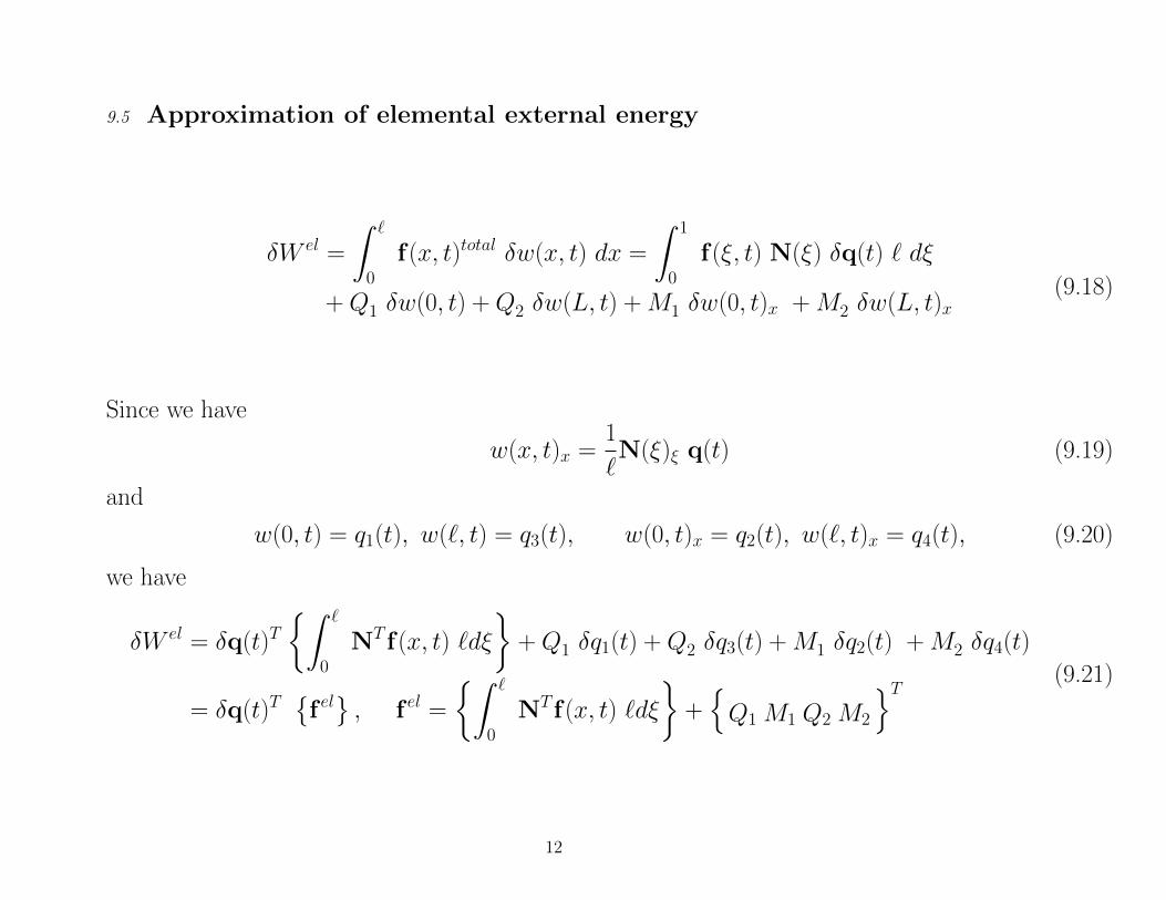
For element 3: q(3) =
q(3)1
q(3)2
=
u3
u4
(9.24)
16

Assembly of the three elements proceeds as follows:
q(1)
q(2)
q(3)
=
I 0 0 0
0 I 0 0
0 I 0 0
0 0 I 0
0 0 I 0
0 0 0 I
u1
u2
u3
u4
⇓
For general case:
q` = L ug
(9.25)
17

9.7.3 Sum up the total system kinetic energy.
T total =
n∑el=1
T el =
12{q(1)}T [m(1)]{q(1)} + 1
2{q(2)}T [m(1)]{q(2)}+... + 1
2{q(n)}T [m(n)]{q(n)}
=
q(1)
q(2)
..
q(n)
T m(1) 0 ... 0
0 m(2) ... 0
0 0 ... 0
0 0 .. m(n)
q(1)
q(2)
..
q(n)
T total = 1
2{q`}T [m] {q`}
(9.26)
18

9.7.4 Sum up the total system strain energy.
V totalb =
n∑el=1
V elb =
12{q(1)}T [k(1)]{q(1)} + 1
2{q(2)}T [k(1)]{q(2)}+... + 1
2{q(n)}T [k(n)]{q(n)}
=
q(1)
q(2)
..
q(n)
T k(1) 0 ... 0
0 k(2) ... 0
0 0 ... 0
0 0 .. k(n)
q(1)
q(2)
..
q(n)
V totalb = 1
2{q`}T [k] {q`}
(9.27)
19

9.7.5 Assembly of the partitioned elements back into a beam.
This corresponds to substituting the partitioned elemental degrees of freedom, q`, by the assembled
(or global) degrees of freedom, ug, via (9.25):
• Total assembled system kinetic energy:
T total = 12{q`}
T [m] {q`} = 12{u
Tg LT}[m] {Lug}
= 12u
Tg [LTm L] ug
T total = 12u
Tg Mg ug, Mg = LTmL
(9.28)
Similarly, for the assembled bending energy we have
V totalb = 1
2{q`}T [k] {q`} = 1
2{uTg LT}[k] {Lug}
= 12u
Tg [LTk L] ug
V totalb = 1
2uTg Kg ug, Kg = LTkL
(9.29)
20

The total external work can be assembled as
δW totalapplied =
n∑el=1
{δq(t)(el)}T {f el}
= δqT` f ` = δuTg {LT f `}
δW total = δuTg f g
(9.30)
21

9.8 Euler-Lagrange’s equations of motion
Lagrangian:
L = T total − V total
= 12u
TgMg ug − 1
2uTgKg ug
(9.31)
Applying the generic Euler-Lagrange equations of motion:
d
dt
∂L
∂qk− ∂L
∂qk= Qk (9.32)
we obtain the FEM equations of motion from (9.30) and (9.31) as
Mg ug + Kg ug = f g (9.33)
22