Finite Element Analysis of Karting Chassis Dynamics and Axle Flexure

Matthew Hodek

Honors Project

Submitted to the University Honors Program At Bowling Green State University in partial

Fulfillment of the requirements for graduation with

UNIVERSITY HONORS

Spring 2007

Dr. Robert Boughton, Advisor Dept of Physics and Astronomy Dr. So-Hsiang Chou, Advisor Dept of Mathematics and Statistics Dr. Tong Sun, Advisor Dept of Mathematics and Statistics

1 Motivation

This study is done in conjunction with Quantum Racing which is part of the Society of PhysicsStudents in the Department of Physics and Astronomy at Bowling Green State University. The kartchassis model is based on the Quantum Racing kart and its typical racing setup as seen in figure 1.

Figure 1: The Quantum Racing kart driven by Jen Bradley in the 2006 Grand Prix of BGSU.

Under the specifications of the Grand Prix of BGSU, all of the karts have a relatively low powerto weight ratio. This evens out the field making it more competitive and exciting. These conditionsmake the handling of the kart and the driver’s technique critical in a team’s chances for success.Both of these fundamentals are directly linked to how the chassis is designed and how it performsunder different racing conditions. Thus it is the main intention of this study to begin to understandand build a model of the chassis dynamics. Another interest of this study is to model the rear axleand attempt to determine if axle flexure was responsible for the mechanical failure of the drive chainsystem of the Quantum Racing kart in the 2006 Grand Prix of BGSU.

2 The Finite Element Method

2.1 Introduction

Many physical systems can be modeled using differential or partial differential equations. As thecomplexity of a system increases the number of equations, and the complexity of the coupling ofthose equations, increases dramatically. This leads to a need for a numerical method to solve thesesystems of equations. In general, the finite element method is a technique to transform a system ofdifferential equations into a system of algebraic equations that can be solved using traditional linearalgebra techniques.

1

2.2 Formulation Overview

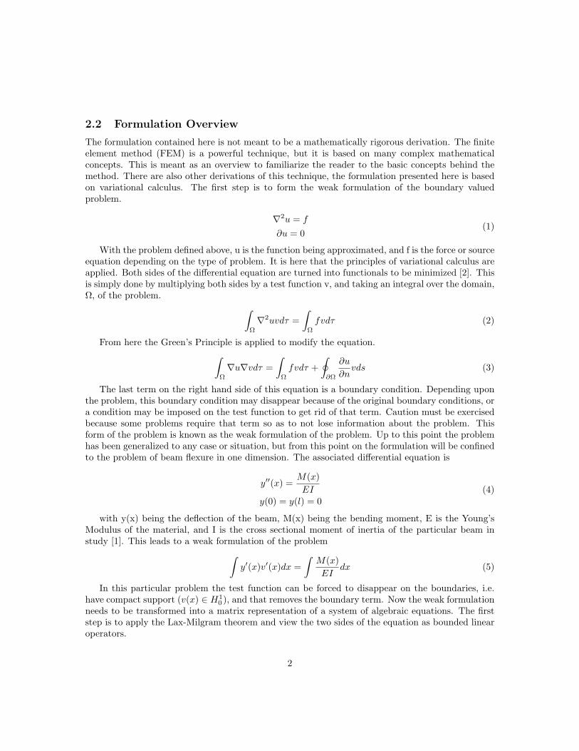
The formulation contained here is not meant to be a mathematically rigorous derivation. The finiteelement method (FEM) is a powerful technique, but it is based on many complex mathematicalconcepts. This is meant as an overview to familiarize the reader to the basic concepts behind themethod. There are also other derivations of this technique, the formulation presented here is basedon variational calculus. The first step is to form the weak formulation of the boundary valuedproblem.

∇2u = f

∂u = 0(1)

With the problem defined above, u is the function being approximated, and f is the force or sourceequation depending on the type of problem. It is here that the principles of variational calculus areapplied. Both sides of the differential equation are turned into functionals to be minimized [2]. Thisis simply done by multiplying both sides by a test function v, and taking an integral over the domain,Ω, of the problem. ∫

Ω

∇2uvdτ =∫

Ω

fvdτ (2)

From here the Green’s Principle is applied to modify the equation.∫Ω

∇u∇vdτ =∫

Ω

fvdτ +∮

∂Ω

∂u

∂nvds (3)

The last term on the right hand side of this equation is a boundary condition. Depending uponthe problem, this boundary condition may disappear because of the original boundary conditions, ora condition may be imposed on the test function to get rid of that term. Caution must be exercisedbecause some problems require that term so as to not lose information about the problem. Thisform of the problem is known as the weak formulation of the problem. Up to this point the problemhas been generalized to any case or situation, but from this point on the formulation will be confinedto the problem of beam flexure in one dimension. The associated differential equation is

y′′(x) =M(x)EI

y(0) = y(l) = 0(4)

with y(x) being the deflection of the beam, M(x) being the bending moment, E is the Young’sModulus of the material, and I is the cross sectional moment of inertia of the particular beam instudy [1]. This leads to a weak formulation of the problem∫

y′(x)v′(x)dx =∫

M(x)EI

dx (5)

In this particular problem the test function can be forced to disappear on the boundaries, i.e.have compact support (v(x) ∈ H1

0 ), and that removes the boundary term. Now the weak formulationneeds to be transformed into a matrix representation of a system of algebraic equations. The firststep is to apply the Lax-Milgram theorem and view the two sides of the equation as bounded linearoperators.

2

a(u, v) = l(v) (6)

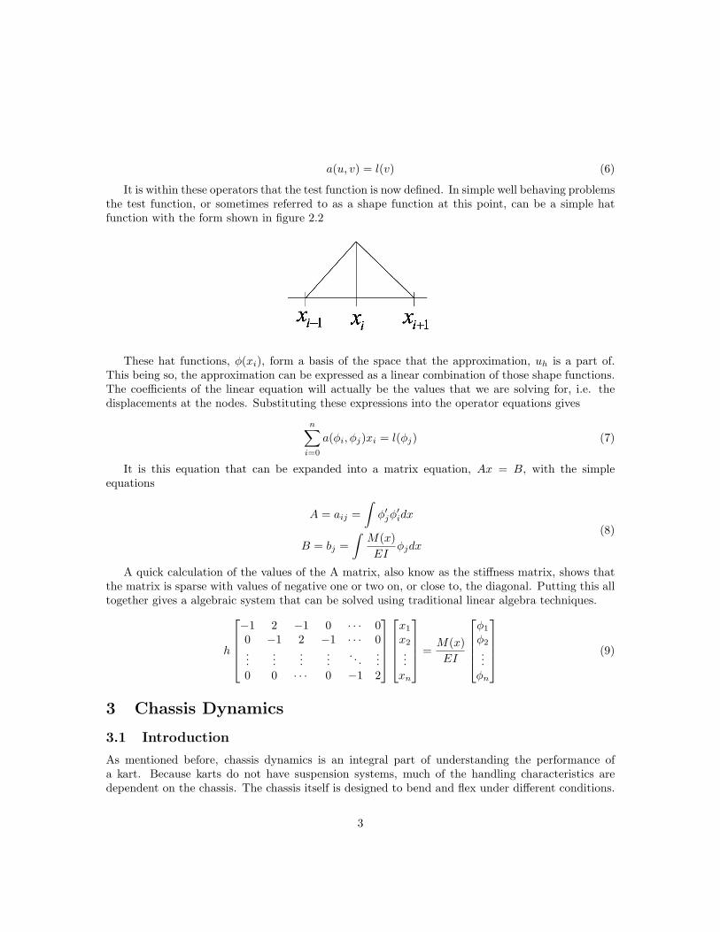
It is within these operators that the test function is now defined. In simple well behaving problemsthe test function, or sometimes referred to as a shape function at this point, can be a simple hatfunction with the form shown in figure 2.2

These hat functions, φ(xi), form a basis of the space that the approximation, uh is a part of.This being so, the approximation can be expressed as a linear combination of those shape functions.The coefficients of the linear equation will actually be the values that we are solving for, i.e. thedisplacements at the nodes. Substituting these expressions into the operator equations gives

n∑i=0

a(φi, φj)xi = l(φj) (7)

It is this equation that can be expanded into a matrix equation, Ax = B, with the simpleequations

A = aij =∫

φ′jφ

′idx

B = bj =∫

M(x)EI

φjdx

(8)

A quick calculation of the values of the A matrix, also know as the stiffness matrix, shows thatthe matrix is sparse with values of negative one or two on, or close to, the diagonal. Putting this alltogether gives a algebraic system that can be solved using traditional linear algebra techniques.

h

−1 2 −1 0 · · · 00 −1 2 −1 · · · 0...

......

.... . .

...0 0 · · · 0 −1 2

x1

x2

...xn

=M(x)EI

φ1

φ2

...φn

(9)

3 Chassis Dynamics

3.1 Introduction

As mentioned before, chassis dynamics is an integral part of understanding the performance ofa kart. Because karts do not have suspension systems, much of the handling characteristics aredependent on the chassis. The chassis itself is designed to bend and flex under different conditions.

3

Of main concern in this study is the weight transfer to different wheels in cornering, and the requiredcoefficient of friction. Two basic handling adjustments will also be explored. Due to the complexityof the kart chassis, a commercially available program called VisualFEA was used for this analysis[4].

3.2 Model Design and Simplifications

To form the model, the chassis of the Quantum Racing kart was mapped out using approximately60 interaction points where two frame members joined. These interaction points would later becomethe nodes for the FEA. Each of these interactions points it assumed to be a solid joint such as aweld. The model used for this study is simplified from the actual kart for a variety of reasons. Thisis a ’first generation’ model and so it serves as a starting point rather than a detailed study. Manyof the simplifications are thought to add second or third order effects. It is hoped that at a latertime these effects can be added into the model and more accurate results can be found.

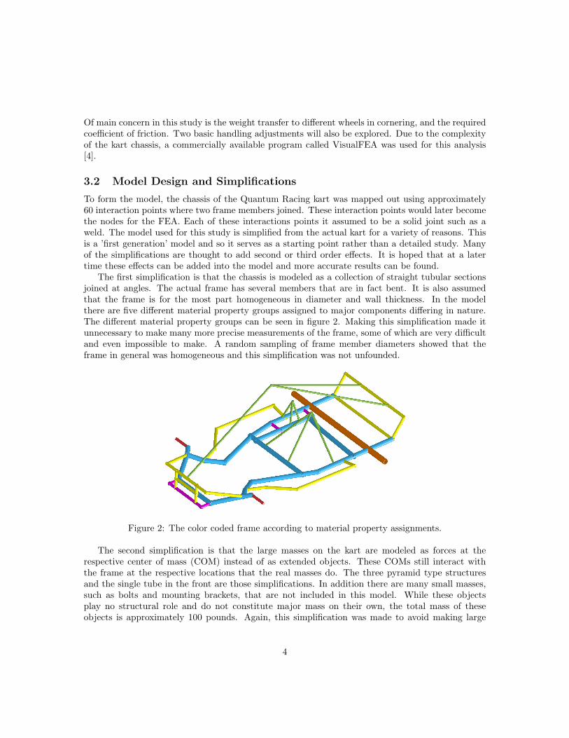
The first simplification is that the chassis is modeled as a collection of straight tubular sectionsjoined at angles. The actual frame has several members that are in fact bent. It is also assumedthat the frame is for the most part homogeneous in diameter and wall thickness. In the modelthere are five different material property groups assigned to major components differing in nature.The different material property groups can be seen in figure 2. Making this simplification made itunnecessary to make many more precise measurements of the frame, some of which are very difficultand even impossible to make. A random sampling of frame member diameters showed that theframe in general was homogeneous and this simplification was not unfounded.

Figure 2: The color coded frame according to material property assignments.

The second simplification is that the large masses on the kart are modeled as forces at therespective center of mass (COM) instead of as extended objects. These COMs still interact withthe frame at the respective locations that the real masses do. The three pyramid type structuresand the single tube in the front are those simplifications. In addition there are many small masses,such as bolts and mounting brackets, that are not included in this model. While these objectsplay no structural role and do not constitute major mass on their own, the total mass of theseobjects is approximately 100 pounds. Again, this simplification was made to avoid making large

4

and complicated sets of precise measurements. A third simplification is that the steering geometryin not included in the model. While the kart is turning through a corner the front end changes itsgeometry to make the turn and create other effects. Again, including these geometry changes wouldrequire large amounts of complicated measurements. Furthermore, it is unknown precisely how andwhen the steering wheel is turned in a corner so including such actions in the model would at bestbe an educated guess. The final simplification is that there are no tires and the axle and spindles arepinned at the center of the tires. Tire and wheel dynamics is a project in its own right and was notconsidered within this study. In the future making measurements of the tire properties may lead tomodeling the tires as springs

3.3 Analysis Process

Once the model is constructed inside the FE program, a series of tests can be performed. All ofthe tests performed were static turns, meaning that it was like a snap shot of the kart at a momentgoing through a turn. The individual turns were classified by their acceleration. This avoids havingto make specifications of the turn geometry and of the kart’s speed. To relate the model data toactual data runs of the kart, a simple formula can be used to calculate the turns acceleration.

a =v2

r(10)

A range of turns from 0 to 1.5 g’s (g = 9.8m/s2) was explored. For each of these accelerationsan associated force was calculated for each of the four COM approximations. The program has abuilt in function for applying an acceleration to the frame elements themselves. Once the problemwas solved by the program for a certain acceleration, the individual reaction forces at each of thewheels was recorded in the X, Y, and Z direction.

3.4 Left Turn

It was arbitrarily chosen to study left hand turns in detail, with a less detailed look at right handturns in the next section. A main goal of these simulations was to see the weight transfer to theoutside wheels in a turn. These being left handed turns, the weight would be transferred to theright side of the kart.

It can be seen in figure 3 that the weight is indeed transferred to the outside wheels in a welldefined linear manner. It is also relevant to note that the kart is balanced left to right whilestationary. At the top of the graph is the total weight of the kart model under the varying turns.The mean total weight of the kart was 268.12 lbs with an average deviation of .02 lbs. While thismeasurement is considerably less than the 367 lbs the Quantum Racing kart was weighted at (asmentioned before), the consistency of the measurement shows the numerical stability of the program.

When the individual wheel weights are plotted in figure 4, a few interesting trends appear. Themost distinguishable feature is that the rear wheels transfer a lot more weight than the front wheelsdo. This is because most of the ’vertical mass’ is located in the rear. Vertical mass refers to massthat lies significantly above the plane of the frame and is the main contributor to weight shift.

One of the more interesting features on this graph is that the inside rear wheel ( the left rear)has a “negative” weight on it in the higher acceleration turns. This indicates that the inside rearwheel is lifting off the ground in those types of turns. This ’rear lift effect’ does indeed happen inkarts as seen in figure 5 but it was thought that the mechanisms that produce this are not included

5

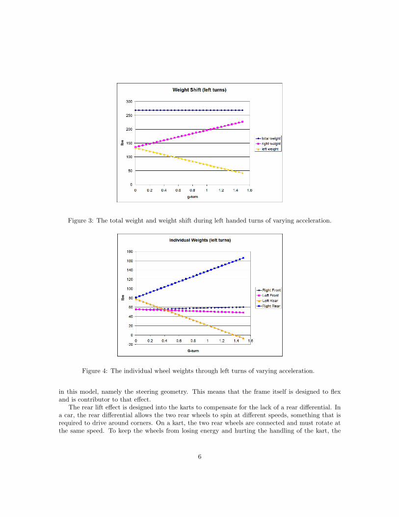
Figure 3: The total weight and weight shift during left handed turns of varying acceleration.

Figure 4: The individual wheel weights through left turns of varying acceleration.

in this model, namely the steering geometry. This means that the frame itself is designed to flexand is contributor to that effect.

The rear lift effect is designed into the karts to compensate for the lack of a rear differential. Ina car, the rear differential allows the two rear wheels to spin at different speeds, something that isrequired to drive around corners. On a kart, the two rear wheels are connected and must rotate atthe same speed. To keep the wheels from losing energy and hurting the handling of the kart, the

6

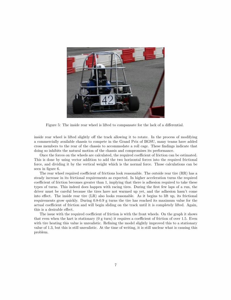
Figure 5: The inside rear wheel is lifted to compansate for the lack of a differential.

inside rear wheel is lifted slightly off the track allowing it to rotate. In the process of modifyinga commercially available chassis to compete in the Grand Prix of BGSU, many teams have addedcross members to the rear of the chassis to accommodate a roll cage. These findings indicate thatdoing so inhibits the natural motion of the chassis and compromises its performance.

Once the forces on the wheels are calculated, the required coefficient of friction can be estimated.This is done by using vector addition to add the two horizontal forces into the required frictionalforce, and dividing it by the vertical weight which is the normal force. Those calculations can beseen in figure 6.

The rear wheel required coefficient of frictions look reasonable. The outside rear tire (RR) has asteady increase in its frictional requirements as expected. In higher acceleration turns the requiredcoefficient of friction becomes greater than 1, implying that there is adhesion required to take thesetypes of turns. This indeed does happen with racing tires. During the first few laps of a run, thedriver must be careful because the tires have not warmed up yet, and the adhesion hasn’t comeinto effect. The inside rear tire (LR) also looks reasonable. As it begins to lift up, its frictionalrequirements grow quickly. During 0.8-0.9 g turns the tire has reached its maximum value for theactual coefficient of friction and will begin sliding on the track until it is completely lifted. Again,this is a desirable effect.

The issue with the required coefficient of friction is with the front wheels. On the graph it showsthat even when the kart is stationary (0 g turn) it requires a coefficient of friction of over 1.5. Evenwith tire heating this value is unrealistic. Refining the model slightly improved this to a stationaryvalue of 1.3, but this is still unrealistic. At the time of writing, it is still unclear what is causing thisproblem.

7

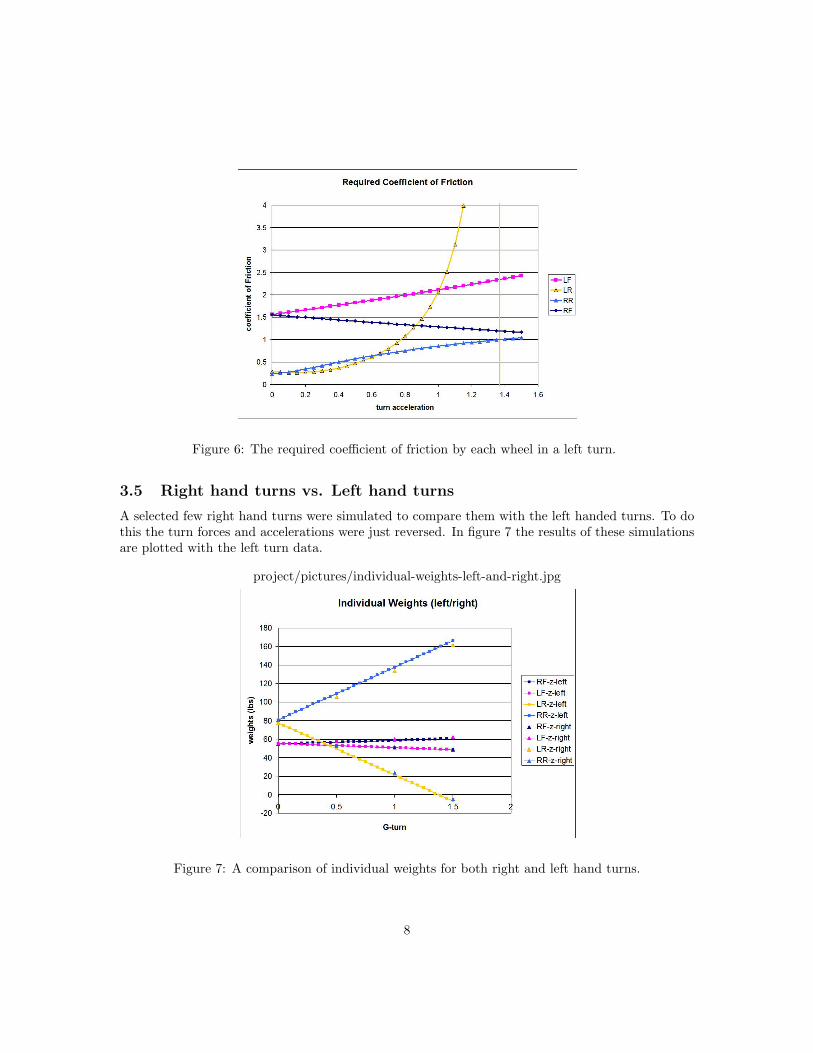
Figure 6: The required coefficient of friction by each wheel in a left turn.

3.5 Right hand turns vs. Left hand turns

A selected few right hand turns were simulated to compare them with the left handed turns. To dothis the turn forces and accelerations were just reversed. In figure 7 the results of these simulationsare plotted with the left turn data.

project/pictures/individual-weights-left-and-right.jpg

Figure 7: A comparison of individual weights for both right and left hand turns.

8

The right hand data is slightly different from the left hand turns, but it seems to follow the samelinear relationship. The biggest difference can be seen in the outside rear wheel in both types ofturns. The weight on the outside rear in the right hand turns is slightly lower than in the left handturns. This is representative of the fact that there is slightly more weight on the right hand sideand it doesn’t transfer as well to the left/outside in a right hand turn. This suggests that on a trackwhere the kart needs to turn equally well on both directions that the kart needs to be set up slightlyasymmetrically. This asymmetry is probably too small to be noticed by a driver, but options willbe discussed in the section on the next section.

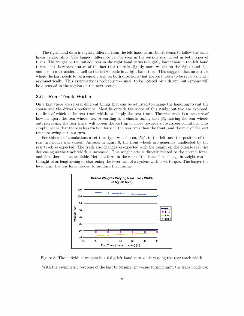
3.6 Rear Track Width

On a kart there are several different things that can be adjusted to change the handling to suit thecourse and the driver’s preference. Most lie outside the scope of this study, but two are explored,the first of which is the rear track width, or simply the rear track. The rear track is a measure ofhow far apart the rear wheels are. According to a chassis tuning text [3], moving the rear wheelsout, increasing the rear track, will loosen the kart up or move towards an oversteer condition. Thissimply means that there is less friction force in the rear tires than the front, and the rear of the karttends to swing out in a turn.

For this set of simulations a set turn type was chosen, .5g’s to the left, and the position of therear tire nodes was varied. As seen in figure 8, the front wheels are generally unaffected by therear track as expected. The track also changes as expected with the weight on the outside rear tiredecreasing as the track width is increased. This weight acts is directly related to the normal force,and thus there is less available frictional force in the rear of the kart. This change in weight can bethought of as lengthening or shortening the lever arm of a system with a set torque. The longer thelever arm, the less force needed to produce that torque.

Figure 8: The individual weights in a 0.5 g left hand turn while varying the rear track width

With the asymmetric response of the kart to turning left versus turning right, the track width can

9

be varied to correct this. Either the left rear can be brought in, or the right rear can be moved out tobalance the kart. However, the current difference in outside weights in a .5 g turn is approximately4 lbs, and according the data the rear track would have to be moved in an amount that couldn’t bephysically possible on the kart. Therefore, this technique to balance the kart is for fine tuning, andballast weight placement should be used for larger changes.

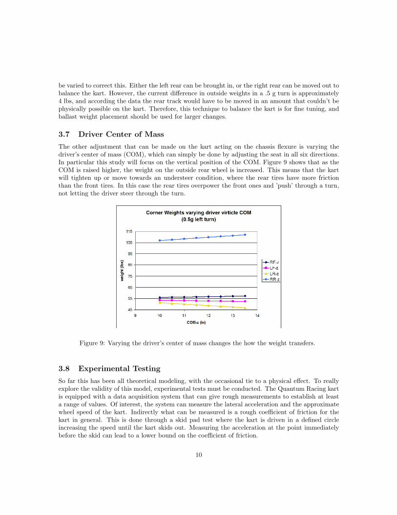
3.7 Driver Center of Mass

The other adjustment that can be made on the kart acting on the chassis flexure is varying thedriver’s center of mass (COM), which can simply be done by adjusting the seat in all six directions.In particular this study will focus on the vertical position of the COM. Figure 9 shows that as theCOM is raised higher, the weight on the outside rear wheel is increased. This means that the kartwill tighten up or move towards an understeer condition, where the rear tires have more frictionthan the front tires. In this case the rear tires overpower the front ones and ’push’ through a turn,not letting the driver steer through the turn.

Figure 9: Varying the driver’s center of mass changes the how the weight transfers.

3.8 Experimental Testing

So far this has been all theoretical modeling, with the occasional tie to a physical effect. To reallyexplore the validity of this model, experimental tests must be conducted. The Quantum Racing kartis equipped with a data acquisition system that can give rough measurements to establish at leasta range of values. Of interest, the system can measure the lateral acceleration and the approximatewheel speed of the kart. Indirectly what can be measured is a rough coefficient of friction for thekart in general. This is done through a skid pad test where the kart is driven in a defined circleincreasing the speed until the kart skids out. Measuring the acceleration at the point immediatelybefore the skid can lead to a lower bound on the coefficient of friction.

10

Due to weather and time constraints within the Grand Prix season this test was only attemptedonce. Due to many reasons within that test session itself including the track surface being roughand technical difficulties with the IR beacons, the test was not successful. There are plans to trythe experiment again in the future.

4 Axle Flexure

4.1 Introduction

In the 2006 Grand Prix of BGSU three of the six competing karts had mechanical failures involvingtheir drive chains derailing. It is thought that axle flexure may have played a role in those events.This part of the study is aimed at seeing what kind of conditions would be necessary for the axle toflex enough to tilt the sprocket out of alignment as seen in figure 10. For this a model was constructedin VisualFEA program [4] and the forces on the axle were varied. Ideally the chassis model wouldprovide approximate forces on the axle, but extracting that information proved difficult. Thereforeconditions were varied to match the rear tire forces on the chassis model.

Figure 10: An over-exaggeration of the axle (grey) flexing and causing the sprocket (red) to be tiltedout of alignmentby and angle θ. The large dots are indicating the sprocket, frame bearing, and wheelnodes from left to right respectively.

4.2 Data and Interpretation

Calculations show that in a 1 g turn, the axle would deflect the sprocket .05 deg from the vertical(θ=0.05). Assuming the largest sprocket radius used by Quantum Racing of 4.067 in, it would deflectthe top of the sprocket .004 in. out of alignment. This is smaller than the gap allowed between thesprocket and the chain meaning that axle flexure alone is not responsible. While these are rough

11

calculations, the angle of deflection of the sprocket node in these calculations, is comparable to theangle of deflection of neighboring nodes in the chassis model.

It is worth while noting that since the 2006 season Quantum Racing has installed a sprocketguard to help keep the chain on the sprocket. After running many laps in the 2007 season, not oncedid the chain derail, nor were there any markings on the sprocket guard to indicate that the chainwas even trying to derail. Changes made to the kart and possible reasons for this good fortune areunder investigation.

5 Acknowledgements

I would personally like to thank my advisors for helping me through this project. It has been anincredible learning experience that will stay with me throughout my physics career. I would like tothank Alex Hann who is the advisor to Quantum Racing for the endless help and direction with theteam. I would also like to thank the entire Department of Physics and Astronomy at Bowling GreenState University for their continued support and encouragement.

A thank you also goes out to the Honors Program of BGSU for providing opportunities andencouraging students to be the best that they can be.

An electronic, full-color version of this paper in PDF format will be available on the QuantumRacing Website at

http://physics.bgsu.edu/Quantum Racing/research undergrad.html

References

[1] Harris, Charles O. Statics and Strength of Materials. New York: John Wiley and Sons, 1982.

[2] Lewis, P.E. and J.P. Ward. The Finite Element Method: Principles and Applications. NewYork: Addison-Wesly Publishing Company, 1991.

[3] Smith, Steven. Kart Chassis Setup Technology. Santa Ana: Steve Smith Autosports Publica-tions, 2005.

[4] VisualFEA. Intuition Software. http://www.visualfea.com

12